Many Sets Have More Sums Than Differences

Greg Martin Email: gerg@math.ubc.ca Affiliation: University of British Columbia Affiliation: and Affiliation: Kevin O’Bryant Email: kevin@member.ams.org Affiliation: City University of New York, Staten Island

1 Introduction

As addition is commutative but subtraction is not, the set of sums

S+S:=\{s_{1}+s_{2}\colon s_{i}\in S\}

of a finite set $S$ is predisposed to be smaller than the set of differences

S-S:=\{s_{1}-s_{2}\colon s_{i}\in S\}.

As Nathanson [4] wrote:

“Even though there exist sets $A$ that have more sums than differences, such sets should be rare, and it must be true with the right way of counting that the vast majority of sets satisfies $|A-A|>|A+A|$ .”

Following this reasoning, one would suspect that a vanishingly small proportion of the $2^{n}$ subsets of $\{0,1,2,\dots,n-1\}$ have more sums than differences. Our purpose, however, is to show that this is not the case. The following terminology will be used throughout this article:

Definition.

A finite set $S$ is difference-dominant if $|S-S|>|S+S|$ , sum-dominant if $|S+S|>|S-S|$ , and sum-difference-balanced if $|S+S|=|S-S|$ .

Nathanson [5] calls sum-dominant sets “MSTD” sets, short for “More Sums Than Differences”. We refer the reader to [4, 5] for the history of this problem.

Our main theorem shows that, perhaps contrary to intuition, all three types of set in the above definition are ubiquitous.

Theorem 1.

Let $P$ be any arithmetic progression of length $n$ . A positive proportion of the subsets of $P$ are difference-dominant, a positive proportion are sum-dominant, and a positive proportion are sum-difference-balanced. More precisely, there exists $c>0$ such that for all $n\geq 15$ ,

	$\displaystyle\#\big\{S\subseteq P$	$\displaystyle:S\text{ is difference-dominant}\big\}>c2^{n},$
	$\displaystyle\#\big\{S\subseteq P$	$\displaystyle:S\text{ is sum-dominant}\big\}>c2^{n},$
	$\displaystyle\#\big\{S\subseteq P$	$\displaystyle:S\text{ is sum-difference-balanced}\big\}>c2^{n}.$

We observe that the sizes of $S+S$ and $S-S$ are invariant under translation and dilation of $S$ , so that without loss of generality we can restrict our attention to $P=\{0,1,2,\dots,n-1\}$ .

The following examples show that none of the three categories is empty for $n\geq 15$ :

Example.

The set $S=\{0,1,3\}$ has $S+S=\{0,1,2,3,4,6\}$ and $S-S=\{-3,-2,-1,0,1,2,3\}$ ; therefore $S$ is difference-dominant, since $|S-S|=7>6=|S+S|$ .

Example.

The set $S=\{0,2,3,4,7,11,12,14\}$ has $S+S=\{0,\dots,28\}\setminus\{1,20,27\}$ and $S-S=\{-14,\dots,14\}\setminus\{-13,-6,6,13\}$ ; therefore $S$ is sum-dominant, since $|S+S|=26>25=|S-S|$ .

Example.

A set $S$ is symmetric if $S=a^{\ast}-S$ for some $a^{\ast}\in{\mathbb{R}}$ . Any symmetric set has $S+S=S+(a^{\ast}-S)=a^{\ast}+(S-S)$ ; therefore symmetric sets are sum-difference-balanced. In particular, any interval or arithmetic progression is sum-difference-balanced.

The idea behind Theorem 1 is the following. Most subsets of $\{0,1,2,\dots,n-1\}$ have about $n/2$ elements; call our typical subset $S$ . Each $k\in\{0,1,2,\dots,2n-2\}$ has, on average, roughly $n/4-|n-k|/4$ representations as a sum of two elements of $S$ . Not only is this positive, it is quite large except when $k$ is near 0 or $2n-2$ . Similarly, each nonzero $k\in\{-(n-1),\dots,n-1\}$ has, on average, roughly $n/4-|k|/4$ representations as a difference of two elements of $S$ . Not only is this positive, it is quite large except when $|k|$ is near $n-1$ . Putting these together, the sizes of the sumset and difference set are predominantly affected by the elements of $S$ that are near 0 or near $n$ . If we choose the “fringe” of $S$ cleverly, the middle of $S$ will become largely irrelevant.

This philosophy suggests the following conjecture; see Section 7 for a more refined conjecture.

Conjecture 2.

Let $P$ be any arithmetic progression with length $n$ . The limiting proportions

	$\displaystyle\rho_{-}$	$\displaystyle=\lim_{n\to\infty}2^{-n}\,\#\big\{S\subseteq P:S\text{ is difference-dominant}\big\}$
	$\displaystyle\rho_{+}$	$\displaystyle=\lim_{n\to\infty}2^{-n}\,\#\big\{S\subseteq P:S\text{ is sum-dominant}\big\}$
	$\displaystyle\rho_{=}$	$\displaystyle=\lim_{n\to\infty}2^{-n}\,\#\big\{S\subseteq P:S\text{ is sum-difference-balanced}\big\}$

all exist and are positive.

The following result, on the other hand, supports Nathanson’s instinct as quoted above, with one interpretation of “the right way” and a suitably humble understanding of “vast”. Theorem 3 is proved in Section 4.

Theorem 3.

Let $P$ be any arithmetic progression with length $n$ . On average, the difference set of a subset of $P$ has 4 more elements than its sumset. More precisely,

	$\displaystyle\frac{1}{2^{n}}\sum_{S\subseteq P}\|S-S\|$	$\displaystyle\sim 2n-7,$
	$\displaystyle\frac{1}{2^{n}}\sum_{S\subseteq P}\|S+S\|$	$\displaystyle\sim 2n-11.$

Nathanson [5] asks for the possible values of $|A+A|-|A-A|$ . We show by construction in Section 5 that the range of $|A+A|-|A-A|$ is $\mathbb{Z}$ ; in fact our constructions are economical, in the sense of the following theorem, which is the subject of Section 5:

Theorem 4.

For every integer $x$ , there is a set $S\subseteq\{0,1,\dots,17|x|\}$ with $|S+S|-|S-S|=x$ .

Acknowledgements. The first author was supported in part by grants from the Natural Sciences and Engineering Research Council. The second author was supported in part by a grant from The City University of New York PSC-CUNY Research Award Program. The second author also acknowledges helpful discussions with Natella V. O’Bryant.

2 Sums and differences in randomly chosen sets

In this section, we establish several ancillary results on the probabilities that particular sums and differences are present or absent in sets chosen randomly from certain classes of sets. We will consider in particular the following classes: Let $n$ , $\ell$ , and $u$ be integers with $n\geq\ell+u$ . Fix $L\subseteq\{0,\dots,\ell-1\}$ and $U\subseteq\{n-u,\dots,n-1\}$ . We will consider the set of all subsets $A\subseteq\{0,\dots,n-1\}$ satisfying $A\cap\{0,\dots,\ell-1\}=L$ and $A\cap\{n-u,\dots,n-1\}=U$ as a probability space endowed with the uniform probability, where each such set $A$ occurs with the probability $2^{-(n-\ell-u)}$ .

All of the calculations in this section are straightforward, but the details depend upon the size and sometimes the parity of the particular sum or difference we are investigating, and so the lemmas herein are rather ugly. The reader with limited tolerance could scan Propositions 8 and 12 and move on to the next section without significantly interrupting the flow of ideas.

We begin with three lemmas describing the probabilities of particular sums missing from $A+A$ , where $A$ is chosen randomly from a class of the type indicated above.

Lemma 5.

Let $n$ , $\ell$ , and $u$ be integers with $n\geq\ell+u$ . Fix $L\subseteq\{0,\dots,\ell-1\}$ and $U\subseteq\{n-u,\dots,n-1\}$ . Suppose that $R$ is a uniformly randomly chosen subset of $\{\ell,\dots,n-u-1\}$ , and set $A:=L\cup R\cup U$ . Then for any integer $k$ satisfying $2\ell-1\leq k\leq n-u-1$ , the probability

{\mathbb{P}}\left[k\notin A+A\right]=\begin{cases}\big(\tfrac{1}{2}\big)^{|L|}\big(\tfrac{3}{4}\big)^{(k+1)/2-\ell},&\text{if $k$ is odd,}\\ \big(\tfrac{1}{2}\big)^{|L|+1}\big(\tfrac{3}{4}\big)^{k/2-\ell},&\text{if $k$ is even.}\\ \end{cases}

Proof.

Define random variables $X_{j}$ by setting $X_{j}=1$ if $j\in A$ and $X_{j}=0$ otherwise. By the definition of $A$ , the variables $X_{j}$ are independent random variables for $\ell\leq j\leq n-u-1$ , each taking the values 0 and 1 with probability $1/2$ each, while the variables $X_{j}$ for $0\leq j\leq\ell-1$ and $n-u\leq j\leq n-1$ have values that are fixed by the choices of $L$ and $U$ .

We have $k\notin A+A$ if and only if $X_{j}X_{k-j}=0$ for all $0\leq j\leq k/2$ ; the key point is that these variables $X_{j}X_{k-j}$ are independent of one another. Therefore

{\mathbb{P}}\left[k\notin A+A\right]=\prod_{0\leq j\leq k/2}{\mathbb{P}}\left[X_{j}X_{k-j}=0\right].

If $k$ is odd, this becomes

	$\displaystyle{\mathbb{P}}\left[k\notin A+A\right]$	$\displaystyle=\prod_{j=0}^{\ell-1}{\mathbb{P}}\left[X_{j}X_{k-j}=0\right]\prod_{j=\ell}^{(k-1)/2}{\mathbb{P}}\left[X_{j}X_{k-j}=0\right]$
		$\displaystyle=\prod_{j\in L}{\mathbb{P}}\left[X_{k-j}=0\right]\prod_{j=\ell}^{(k-1)/2}{\mathbb{P}}\left[X_{j}=0\text{ or }X_{k-j}=0\right]$
		$\displaystyle=\big(\tfrac{1}{2}\big)^{\|L\|}\big(\tfrac{3}{4}\big)^{(k+1)/2-\ell}.$

On the other hand, if $k$ is even then

	$\displaystyle{\mathbb{P}}\left[k\notin A+A\right]$	$\displaystyle=\prod_{j=0}^{\ell-1}{\mathbb{P}}\left[X_{j}X_{k-j}=0\right]\bigg(\prod_{j=\ell}^{k/2-1}{\mathbb{P}}\left[X_{j}X_{k-j}=0\right]\bigg){\mathbb{P}}\left[X_{k/2}X_{k/2}=0\right]$
		$\displaystyle=\prod_{j\in L}{\mathbb{P}}\left[X_{k-j}=0\right]\bigg(\prod_{j=\ell}^{k/2-1}{\mathbb{P}}\left[X_{j}=0\text{ or }X_{k-j}=0\right]\bigg){\mathbb{P}}\left[X_{k/2}=0\right]$
		$\displaystyle=\big(\tfrac{1}{2}\big)^{\|L\|}\big(\tfrac{3}{4}\big)^{k/2-\ell}\cdot\tfrac{1}{2}.$

∎

Lemma 6.

{\mathbb{P}}\left[k\notin A+A\right]=\begin{cases}\big(\tfrac{1}{2}\big)^{|U|}\big(\tfrac{3}{4}\big)^{n-(k+1)/2-u},&\text{if $k$ is odd,}\\ \big(\tfrac{1}{2}\big)^{|U|+1}\big(\tfrac{3}{4}\big)^{n-1-k/2-u},&\text{if $k$ is even.}\\ \end{cases}

Proof.

This follows from Lemma 5 applied to the parameters $\ell^{\prime}=u$ and $L^{\prime}=n-1-U$ , $u^{\prime}=\ell$ and $U^{\prime}=n-1-L$ , and $A^{\prime}=n-1-A$ and $k^{\prime}=2n-2-k$ . ∎

Lemma 7.

Suppose that $A$ is a uniformly randomly chosen subset of $\{0,\dots,n-1\}$ . Then for any integer $0\leq k\leq n-1$ , the probability

{\mathbb{P}}\left[k\notin A+A\right]=\begin{cases}\big(\tfrac{3}{4}\big)^{(k+1)/2},&\text{if $k$ is odd,}\\ \tfrac{1}{2}\big(\tfrac{3}{4}\big)^{k/2},&\text{if $k$ is even;}\\ \end{cases}

while for any integer $n-1\leq k\leq 2n-2$ , the probability

{\mathbb{P}}\left[k\notin A+A\right]=\begin{cases}\big(\tfrac{3}{4}\big)^{n-(k+1)/2},&\text{if $k$ is odd,}\\ \tfrac{1}{2}\big(\tfrac{3}{4}\big)^{n-1-k/2},&\text{if $k$ is even.}\\ \end{cases}

Proof.

This follows immediately from Lemmas 5 and 6 upon setting $\ell=u=0$ and $L=U=\emptyset$ . ∎

We now use these lemmas to establish the following proposition, in which we want a positive probability that many integers $k$ appear in the sumset $A+A$ . While these events, varying over $k$ , are not independent, we need only a lower bound on the probability; hence it suffices to combine crudely the exact probabilities given in Lemmas 5 and 6. We emphasize that we have made no effort to optimize the lower bound given in the following proposition.

Proposition 8.

\{2\ell-1,\dots,n-u-1\}\cup\{n+\ell-1,\dots,2n-2u-1\}\subseteq A+A

is greater than $1-6(2^{-|L|}+2^{-|U|})$ .

Proof.

We employ the crude inequality

{\mathbb{P}}\left[\{2\ell-1,\dots,n-u-1\}\cup\{n+\ell-1,\dots,2n-2u-1\}\not\subseteq A+A\right]\\ \leq\sum_{k=2\ell-1}^{n-u-1}{\mathbb{P}}\left[k\notin A+A\right]+\sum_{k=n+\ell-1}^{2n-2u-1}{\mathbb{P}}\left[k\notin A+A\right].

The first sum can be bounded, using Lemma 5, by

	$\displaystyle\sum_{k=2\ell-1}^{n-u-1}{\mathbb{P}}\left[k\notin A+A\right]$	$\displaystyle<\sum_{\begin{subarray}{c}k\geq 2\ell-1\\ k\text{ odd}\end{subarray}}\big(\tfrac{1}{2}\big)^{\|L\|}\big(\tfrac{3}{4}\big)^{(k+1)/2-\ell}+\sum_{\begin{subarray}{c}k\geq 2\ell-1\\ k\text{ even}\end{subarray}}\big(\tfrac{1}{2}\big)^{\|L\|+1}\big(\tfrac{3}{4}\big)^{k/2-\ell}$
		$\displaystyle=\big(\tfrac{1}{2}\big)^{\|L\|}\sum_{m=0}^{\infty}\big(\tfrac{3}{4}\big)^{m}+\big(\tfrac{1}{2}\big)^{\|L\|+1}\sum_{m=0}^{\infty}\big(\tfrac{3}{4}\big)^{m}=6\big(\tfrac{1}{2}\big)^{\|L\|}.$

The second sum can be bounded in a similar way using Lemma 6, yielding

\sum_{k=n+\ell-1}^{2n-2u-1}{\mathbb{P}}\left[k\notin A+A\right]<6\big(\tfrac{1}{2}\big)^{|U|}.

Therefore ${\mathbb{P}}\left[\{2\ell-1,\dots,n-u-1\}\cup\{n+\ell-1,\dots,2n-2u-1\}\not\subseteq A+A\right]$ is bounded above by $6(1/2)^{|L|}+6(1/2)^{|U|}$ , which is equivalent to the statement of the proposition. ∎

We turn now to three lemmas describing the probabilities that particular differences are missing from $A-A$ , where $A$ is chosen randomly from one of our classes. A new obstacle appears: while the random variables $X_{j}X_{k-j}$ controlling the presence of the sum $k$ in $A+A$ are always mutually independent, the same is not true of the random variables $X_{j}X_{k+j}$ controlling the presence of the difference $k$ in $A-A$ , at least when $k$ is small enough that $j$ , $k+j$ , and $2k+j$ can all lie between 0 and $n-1$ . Fortunately, when $k$ is this small the probabilities in question are already minuscule, so a simple argument provides a serviceable bound (Lemma 10 below).

Lemma 9.

{\mathbb{P}}\left[k\notin A-A\right]=\big(\tfrac{1}{2}\big)^{|L|+|U|}\big(\tfrac{3}{4}\big)^{n-\ell-u-k}.

Proof.

Define random variables $X_{j}$ by setting $X_{j}=1$ if $j\in A$ and $X_{j}=0$ otherwise, as in the proof of Lemma 5. We have $k\notin A-A$ if and only if $X_{j}X_{k+j}=0$ for all $0\leq j\leq n-1-k$ , and again these variables $X_{j}X_{k+j}$ are independent of one another. Therefore

	$\displaystyle{\mathbb{P}}\left[k\notin A-A\right]$	$\displaystyle=\prod_{j=0}^{n-1-k}{\mathbb{P}}\left[X_{j}X_{k+j}=0\right]$
		$\displaystyle=\prod_{j=0}^{\ell-1}{\mathbb{P}}\left[X_{j}X_{k+j}=0\right]\prod_{j=\ell}^{n-u-1-k}{\mathbb{P}}\left[X_{j}X_{k+j}=0\right]\prod_{j=n-u-k}^{n-1-k}{\mathbb{P}}\left[X_{j}X_{k+j}=0\right]$
		$\displaystyle=\prod_{j\in L}{\mathbb{P}}\left[X_{k+j}=0\right]\prod_{j=\ell}^{n-u-1-k}{\mathbb{P}}\left[X_{j}=0\text{ or }X_{k+j}=0\right]\prod_{j\in U-k}{\mathbb{P}}\left[X_{j}=0\right]$
		$\displaystyle=\big(\tfrac{1}{2}\big)^{\|L\|}\big(\tfrac{3}{4}\big)^{n-\ell-u-k}\big(\tfrac{1}{2}\big)^{\|U\|}.$

∎

Lemma 10.

Let $a$ and $b$ be integers with $a<b$ . Suppose that $R$ is a uniformly randomly chosen subset of $\{a,\dots,b-1\}$ . Then for any integer $k$ satisfying $1\leq k\leq 2(b-a)/3$ , the probability

{\mathbb{P}}\left[k\notin R-R\right]\leq\big(\tfrac{3}{4}\big)^{(b-a)/3}.

Remark.

In fact, the probability in question can be written exactly in terms of products of Fibonacci numbers: in the simplest case, ${\mathbb{P}}\left[1\notin R-R\right]=F_{b-a+2}/2^{b-a}$ . However, the resulting expressions would become too tedious to handle in our applications below. When $b-a$ is large and $k$ is small, the actual value of the probability ${\mathbb{P}}\left[k\notin R-R\right]$ is proportional to $((1+\sqrt{5})/4)^{b-a-k}\approx 0.809^{b-a}$ , whereas the bound in Lemma 9 gives $(3/4)^{(b-a)/3}\approx 0.909^{b-a}$ . However, in the particular case $k=(b-a)/2$ , the probability in question is exactly $(3/4)^{(b-a)/2}\approx 0.866^{b-a}$ , so the bound in Lemma 9 is not too unreasonable.

Proof.

Define the set

J:=\big\{a\leq j<b-k:\big\lfloor\tfrac{j-a}{k}\big\rfloor\text{ is even}\big\}.

In other words, $J$ contains the first $k$ integers starting at $a$ , then omits the following $k$ integers, then contains the next $k$ integers, and so on until the upper bound $a+2(b-a)/3$ is reached. The following properties of $J$ can be easily verified:

(i)

if $j\in J$ , then $j+k\notin J$ ;
(ii)

$|J|\geq(b-a)/3$ .

Now define random variables $X_{j}$ by setting $X_{j}=1$ if $j\in R$ and $X_{j}=0$ otherwise, as in the proof of Lemma 10. We have $k\notin R-R$ if and only if $X_{j}X_{k+j}=0$ for all $a\leq j<b-k$ .

	$\displaystyle{\mathbb{P}}\left[k\notin R-R\right]$	$\displaystyle={\mathbb{P}}\left[X_{j}X_{k+j}=0\text{ for all }a\leq j<b-k\right]$
		$\displaystyle\leq{\mathbb{P}}\left[X_{j}X_{k+j}=0\text{ for all }j\in J\right].$

However, property (i) above ensures that the random variables $X_{j}X_{k+j}$ are independent of one another as $j$ ranges over $J$ . Therefore

{\mathbb{P}}\left[k\notin R-R\right]\leq\prod_{j\in J}{\mathbb{P}}\left[X_{j}X_{k+j}=0\right]=\big(\tfrac{3}{4}\big)^{|J|}\leq\big(\tfrac{3}{4}\big)^{(b-a)/3}

by property (ii) above. ∎

Lemma 11.

Suppose that $A$ is a uniformly randomly chosen subset of $\{0,\dots,n-1\}$ . Then for any integer $1\leq k\leq n/2$ , the probability ${\mathbb{P}}\left[k\notin A-A\right]\leq(3/4)^{n/3}$ , while for any integer $n/2\leq k\leq n-1$ , the probability ${\mathbb{P}}\left[k\notin A-A\right]=(3/4)^{n-k}$ .

Proof.

The first assertion follows immediately from Lemma 10 upon setting $a=0$ and $b=n$ , while the second assertion follows immediately from Lemma 9 upon setting $\ell=u=0$ and $L=U=\emptyset$ . ∎

We now use these lemmas to establish the following proposition, in which we want a positive probability that many integers $k$ appear in the difference set $A-A$ . Again it suffices to combine crudely the results of Lemmas 9 and 10, since we need only a lower bound on the probability. Once again we have emphasized ease of exposition over optimization of the lower bound itself; in particular, we could have achieved better constants at the expense of uglier technicalities.

Proposition 12.

Let $n$ , $\ell$ , and $u$ be integers with $n\geq 4(\ell+u)$ . Fix $L\subseteq\{0,\dots,\ell-1\}$ and $U\subseteq\{n-u,\dots,n-1\}$ . Suppose that $R$ is a uniformly randomly chosen subset of $\{\ell,\dots,n-u-1\}$ , and set $A:=L\cup R\cup U$ . Then the probability that

\{-(n-\ell-u),\dots,n-\ell-u\}\subseteq A-A

is greater than $1-4(1/2)^{|L|+|U|}-(n/2)(3/4)^{(n-\ell-u)/3}$ .

Proof.

By the symmetry of $A-A$ about 0 and the fact that $0\in A-A$ for any nonempty set $A$ , it suffices to show that $A-A$ contains $\{1,\dots,n-\ell-u\}$ . We employ the crude inequality

	$\displaystyle{\mathbb{P}}\left[\{1,\dots,n-\ell-u\}\not\subseteq A-A\right]$	$\displaystyle\leq\sum_{k=1}^{n-\ell-u}{\mathbb{P}}\left[k\notin A-A\right]$
		$\displaystyle\leq\sum_{1\leq k\leq n/2}{\mathbb{P}}\left[k\notin R-R\right]+\sum_{n/2<k\leq n-\ell-u}{\mathbb{P}}\left[k\notin A-A\right].$

The first sum can be bounded using Lemma 10 with $a=\ell$ and $b=n-u$ ; it is here that we use the hypothesis $n\geq 4(\ell+u)$ , to guarantee that every $k$ in the range $1\leq k\leq n/2$ satisfies $k\leq 2(n-\ell-u)/3$ . We obtain

\sum_{1\leq k\leq n/2}{\mathbb{P}}\left[k\notin R-R\right]\leq\tfrac{n}{2}\big(\tfrac{3}{4}\big)^{(n-\ell-u)/3}.

The second sum can be bounded using Lemma 6, yielding

\sum_{n/2<k\leq n-\ell-u}{\mathbb{P}}\left[k\notin A-A\right]<\sum_{k=-\infty}^{n-\ell-u}\big(\tfrac{1}{2}\big)^{|L|+|U|}\big(\tfrac{3}{4}\big)^{n-\ell-u-k}=4\big(\tfrac{1}{2}\big)^{|L|+|U|}.

Therefore ${\mathbb{P}}\left[\{-(n-\ell-u),\dots,n-\ell-u\}\not\subseteq A-A\right]$ is bounded above by $4(1/2)^{|L|+|U|}+(n/2)(3/4)^{(n-\ell-u)/3}$ , which is equivalent to the statement of the proposition. ∎

3 Proof of Theorem 1

In this section we show that the collections of sum-dominant sets, difference-dominant sets, and sum-difference-balanced sets all have positive lower density. Our strategy is to fix the “fringes” of a subset of $\{0,1,2,\dots,n-1\}$ (that is, stipulate which integers close to 0 and $n-1$ are and are not in the set) in a way that forces the set to have missing differences (or sums). We then use the probabilistic lemmas of the previous section to show that for many sets with the prescribed fringes, all other sums (or differences) will be present. We have not attempted to optimize the constants appearing in the following three theorems, in part because the previous section would have become even more technical and ugly, and in part because we were unlikely to have come close to the true constants (see Conjecture 18 below) in any event.

We begin by showing that a positive proportion of sets are sum-dominant. Here, choosing appropriate fringes is most non-trivial, compared to the two theorems that follow.

Theorem 13.

For $n\geq 15$ , the number of sum-dominant subsets of $\{0,1,2,\dots,n-1\}$ is at least $(2\times 10^{-7})2^{n}$ .

Proof.

First, note that the bound $(2\times 10^{-7})2^{n}$ is less than 1 for $15\leq n\leq 22$ ; the existence of the single sum-dominant set $\{0,2,3,4,7,11,12,14\}$ is enough to verify the theorem in that range. Henceforth we can assume that $n\geq 23$ .

Define $L:=\{0,2,3,7,8,9,10\}$ and $U:=\{n-11,n-10,n-9,n-8,n-6,n-3,n-2,n-1\}$ . We show that the number of sum-dominant subsets $A\subseteq\{0,1,2,\dots,n-1\}$ satisfying $A\cap\{0,\dots,10\}=L$ and $A\cap\{n-11,\dots,n-1\}=U$ is at least $(2\times 10^{-7})2^{n}$ . For any such $A$ , the fact that $U-L$ does not contain $n-7$ implies that $A-A$ contains neither $n-7$ nor $-(n-7)$ ; since $A-A\subseteq\{-(n-1),\dots,n-1\}$ , we see that

|A-A|\leq 2n-3.

Therefore it suffices to show that there are at least $(2\times 10^{-7})2^{n}$ sets $A$ , satisfying $A\cap\{0,\dots,10\}=L$ and $A\cap\{n-11,\dots,n-1\}=U$ , for which $|A+A|\geq 2n-2$ .

For any such $A$ , we see by direct calculation that $A+A$ contains

	$\displaystyle L+L$	$\displaystyle=\{0,\dots,20\}\setminus\{1\},$
	$\displaystyle L+U$	$\displaystyle=\{n-11,\dots,n+9\},$
	$\displaystyle U+U$	$\displaystyle=\{2n-22,\dots,2n-2\}.$

In particular, if $23\leq n\leq 32$ then $A+A$ automatically equals $\{0,\dots,2n-2\}\setminus\{1\}$ , giving $|A+A|=2n-2$ ; the number of such $A$ is exactly $2^{n-22}>(2\times 10^{-7})2^{n}$ , since there are $n-22$ numbers between 11 and $n-12$ inclusive.

For $n\geq 33$ , Proposition 8 (applied with $\ell=r=11$ ) tells us that when $A$ is chosen uniformly randomly from all such sets, the probability that $A+A$ contains $\{21,\dots,n-12\}\cup\{n+10,\dots,2n-23\}$ is at least

1-6(2^{-|L|}+2^{-|U|})=1-6(2^{-7}+2^{-8})=\frac{119}{128}.

In other words, there are at least $2^{n-22}\cdot 119/128>(2\times 10^{-7})2^{n}$ such sets $A$ . For all these sets, we see that $A+A$ again equals $\{0,\dots,2n-2\}\setminus\{1\}$ , and hence all such sets are sum-dominant. ∎

The next two theorems carry out a similar approach to showing that a positive proportion of sets are difference-dominant or sum-difference-balanced. These two results appeal to the serviceable but crude Lemma 10, and consequently the constants that appear, as well as the computation needed to take care of smaller values of $n$ , are likewise far from optimal.

Theorem 14.

For $n\geq 4$ , the number of difference-dominant subsets of $\{0,1,2,\dots,n-1\}$ is at least $0.0015\cdot 2^{n}$ .

Proof.

The bound can be verified computationally for small $n$ : we have computed by exhaustive search for $n\leq 27$ the number of difference-dominant subsets $\{0,1,2,\dots,n-1\}$ that contain both 0 and $n-1$ . Counting just these sets and their translates is enough to prove this theorem for $n\leq 39$ . Henceforth, we assume that $n\geq 40$ .

Define $L:=\{0,2,3\}$ and $U:=\{n-2,n-1\}$ . We show that the number of difference-dominant subsets $A\subseteq\{0,1,2,\dots,n-1\}$ satisfying $A\cap\{0,1,2,3\}=L$ and $A\cap\{n-2,n-1\}=U$ is at least $0.0015\cdot 2^{n}$ . For any such $A$ , the fact that $L+L$ does not contain 1 implies that $A+A$ does not contain 1, and so $|A+A|\leq 2n-2$ . Therefore it suffices to show that there are at least $0.0015\cdot 2^{n}$ sets $A$ , satisfying $A\cap\{0,1,2,3\}=L$ and $A\cap\{n-2,n-1\}=U$ , for which $|A-A|=2n-1$ .

For any such $A$ , we see by direct calculation that $A-A$ contains

(L-U)\cup(U-L)=\{-(n-5),\dots,-(n-1)\}\cup\{n-5,\dots,n-1\}.

Furthermore, Proposition 12 (applied with $\ell=4$ , $u=2$ , and $n\geq 24$ ) tells us that when $A$ is chosen uniformly randomly from all such sets, the probability that $A-A$ contains $\{-(n-6),\dots,n-6\}$ is at least

	$\displaystyle 1-4\bigg(\frac{1}{2}\bigg)^{\|L\|+\|U\|}-\bigg(\frac{n}{2}\bigg)\bigg(\frac{3}{4}\bigg)^{(n-\ell-u)/3}$	$\displaystyle=1-4\bigg(\frac{1}{2}\bigg)^{5}-\bigg(\frac{n}{2}\bigg)\bigg(\frac{3}{4}\bigg)^{(n-6)/3}$
		$\displaystyle=\frac{7}{8}-\frac{8n}{9}\bigg(\frac{3}{4}\bigg)^{n/3}.$

As a function of $n$ , this expression is increasing for $n\geq 11$ , and at $n=40$ its value is larger than $0.107536$ . In other words, there are at least $2^{n-6}\cdot 0.107536>0.0015\cdot 2^{n}$ such sets $A$ . For all these sets, we see that $A-A$ equals $\{-(n-1),\dots,n-1\}$ , and hence all such sets are difference-dominant. ∎

Theorem 15.

For $n\geq 1$ , the number of sum-difference-balanced subsets of $\{0,1,2,\dots,n-1\}$ is at least $(2\times 10^{-5})2^{n}$ .

Proof.

The bound can be verified computationally for small $n$ : for $n\leq 27$ we have computed the exact number of sum-difference-balanced subsets of $\{0,1,2,\dots,n-1\}$ that contain both $0$ and $n-1$ . Counting only these sets and their translates proves the theorem for $n\leq 42$ . Henceforth, we assume that $n\geq 43$ .

Define $L:=\{0,\dots,5\}$ and $U:=\{n-6,\dots,n-1\}$ . We give a lower bound for the number of sum-difference-balanced subsets $A\subseteq\{0,1,2,\dots,n-1\}$ satisfying $L\cup U\subseteq A$ ; in fact we show that the number of such subsets with $|A+A|=|A-A|=2n-1$ , the maximum possible size, is at least $(2\times 10^{-5})2^{n}$ . Combining Propositions 8 and 12 (applied with $\ell=u=6$ ), we find that when $A$ is chosen uniformly randomly from all such sets, the probability that both $A+A$ and $A-A$ are as large as possible is at least

1-6(2^{-|L|}+2^{-|R|})-4\bigg(\frac{1}{2}\bigg)^{|L|+|U|}-\bigg(\frac{n}{2}\bigg)\bigg(\frac{3}{4}\bigg)^{(n-\ell-u)/3}=\frac{3}{4}-\frac{8n}{9}\bigg(\frac{3}{4}\bigg)^{n/3}.

This function is increasing for $n\geq 1$ and takes a value larger than 0.131232 when $n=43$ . In other words, there are at least $2^{n-12}\cdot 0.131232>(2\times 10^{-5})2^{n}$ such sets $A$ . For all these sets, we see that $A+A$ equals $\{0,\dots,2n-2\}$ and $A-A$ equals $\{-(n-1),\dots,n-1\}$ , and hence all such sets are sum-difference-balanced. ∎

4 Average values

In this section, we prove Theorem 3 by calculating the average values of $|S-S|$ and $|S+S|$ as $S$ ranges over an arithmetic progression $P$ of length $n$ . Since the problem is invariant under dilations and translations, it suffices to prove the theorem in the case $P=\{0,1,2,\dots,n-1\}$ .

We begin by addressing the average cardinality of the sumset $S+S$ . In fact, we can give an exact formula for the average size of the sumset, or equivalently for the sum of the sizes of all sumsets as $S$ ranges over subsets of $\{0,1,2,\dots,n-1\}$ . The reason we can do so is essentially because of the linearity of expectations of random variables.

Theorem 16.

For any positive integer $n$ , we have

\sum_{S\subseteq\{0,\dots,n-1\}}|S+S|=2^{n}(2n-11)+\begin{cases}19\cdot 3^{(n-1)/2},&\text{if $n$ is odd,}\\ 11\cdot 3^{n/2},&\text{if $n$ is even.}\end{cases}

(1)

Proof.

We begin with the manipulation

\sum_{S\subseteq\{0,\dots,n-1\}}|S+S|=\sum_{S\subseteq\{0,\dots,n-1\}}\sum_{\begin{subarray}{c}0\leq k\leq 2n-2\\ k\in S+S\end{subarray}}1=\sum_{k=0}^{2n-2}\sum_{\begin{subarray}{c}S\subseteq\{0,\dots,n-1\}\\ k\in S+S\end{subarray}}1\\ =\sum_{k=0}^{2n-2}2^{n}{\mathbb{P}}\left[k\in S+S\right]=2^{n}(2n-1)-2^{n}\sum_{k=0}^{2n-2}{\mathbb{P}}\left[k\notin S+S\right].

(2)

We suppose that $n=2m+1$ is odd, the case where $n$ is even being similar. We begin by considering only the lower half of possible values for $k$ . By Lemma 7, we have

	$\displaystyle\sum_{k=0}^{n-2}{\mathbb{P}}\left[k\notin S+S\right]$	$\displaystyle=\sum_{j=0}^{m-1}{\mathbb{P}}\left[2j\notin S+S\right]+\sum_{j=0}^{m-1}{\mathbb{P}}\left[2j+1\notin S+S\right]$
		$\displaystyle=\sum_{j=0}^{m-1}\tfrac{1}{2}\big(\tfrac{3}{4}\big)^{j}+\sum_{j=0}^{m-1}\big(\tfrac{3}{4}\big)^{j+1}=5\big(1-\big(\tfrac{3}{4}\big)^{m}\big).$

By the symmetry of $S+S$ about $n-1$ , the same calculation holds for $\sum_{k=n}^{2n-2}{\mathbb{P}}\left[k\notin S+S\right]$ . Therefore, appealing to Lemma 7 again for $k=n-1=2m$ ,

\sum_{k=0}^{2n-2}{\mathbb{P}}\left[k\notin S+S\right]=5\big(1-\big(\tfrac{3}{4}\big)^{m}\big)+\tfrac{1}{2}\big(\tfrac{3}{4}\big)^{m}+5\big(1-\big(\tfrac{3}{4}\big)^{m}\big)=10-\tfrac{19}{2}\big(\tfrac{3}{4}\big)^{(n-1)/2}.

Inserting this value into the right-hand side of equation (2) establishes the lemma for odd $n$ . A similar calculation gives the result for even $n$ . ∎

While it is possible to write down an exact formula for the average size of the difference set $S-S$ as $S$ ranges over all subsets of $\{0,1,2,\dots,n-1\}$ , the formula would be far too ugly to be of use. We prefer in this case to present a simple asymptotic formula with a reasonable error term.

Theorem 17.

For any positive integer $n$ , we have

\sum_{S\subseteq\{0,\dots,n-1\}}|S-S|=2^{n}(2n-7)+O\big(n6^{n/3}\big).

(3)

Proof.

As in the proof of the previous theorem, we have

$\displaystyle\sum_{S\subseteq\{0,\dots,n-1\}}\|S-S\|$	$\displaystyle=\sum_{S\subseteq\{0,\dots,n-1\}}\sum_{\begin{subarray}{c}-(n-1)\leq k\leq n-1\\ k\in S-S\end{subarray}}1=\sum_{k=-(n-1)}^{n-1}\sum_{\begin{subarray}{c}S\subseteq\{0,\dots,n-1\}\\ k\in S-S\end{subarray}}1$
	$\displaystyle=\sum_{k=-(n-1)}^{n-1}2^{n}{\mathbb{P}}\left[k\in S-S\right]$
	$\displaystyle=2^{n}(2n-1)-2^{n}\sum_{k=-(n-1)}^{n-1}{\mathbb{P}}\left[k\notin S-S\right]$
	$\displaystyle=2^{n}(2n-1)-1-2^{n+1}\sum_{k=1}^{n-1}{\mathbb{P}}\left[k\notin S-S\right],$	(4)

the last equality following from the symmetry of $S-S$ around 0 and the fact that 0 is in $S-S$ for nonempty $S$ . From Lemma 11 we have

\sum_{k=1}^{\lceil n/2\rceil-1}{\mathbb{P}}\left[k\notin S-S\right]\leq\sum_{k=1}^{\lceil n/2\rceil-1}\big(\tfrac{3}{4}\big)^{n/3}\leq n\big(\tfrac{3}{4}\big)^{n/3}

and

\sum_{k=\lceil n/2\rceil}^{n-1}{\mathbb{P}}\left[k\notin S-S\right]=\sum_{k=\lceil n/2\rceil}^{n-1}\big(\tfrac{3}{4}\big)^{n-k}=3\big(1-\big(\tfrac{3}{4}\big)^{n-\lceil n/2\rceil}\big),

which combine to give

\sum_{k=1}^{n-1}{\mathbb{P}}\left[k\notin S-S\right]=3+O\big(n\big(\tfrac{3}{4}\big)^{n/3}\big).

Inserting this expression into the right-hand side of equation (4) establishes the theorem. ∎

Examining the derivations of these two theorems reveals that it really is the commutativity $s_{1}+s_{2}=s_{2}+s_{1}$ that causes the difference in the average sizes of $S+S$ and $S-S$ : a typical potential element of $S+S$ has only about half as many chances to be realized as a sum as the corresponding potential element of $S-S$ has at being realized as a difference. To further emphasize this observation, we note that if the single set $S$ is replaced by two sets $S$ and $T$ , the disparity disappears: for an arithmetic progression $P$ of length $n$ , we have

\frac{1}{2^{2n}}\sum_{S\subseteq P}\sum_{T\subseteq P}|S-T|\sim\frac{1}{2^{2n}}\sum_{S\subseteq P}\sum_{T\subseteq P}|S+T|\sim 2n-7.

5 Sets with prescribed imbalance between sums and differences

In this section we prove that the range of possible values for $|S+S|-|S-S|$ is all of ${\mathbb{Z}}$ . Furthermore, as asserted in Theorem 4, our constructions show that for every integer $x$ , we can find a subset $S$ of $\{0,\dots,17|x|\}$ such that $|S+S|-|S-S|=x$ . As one might expect from the foregoing discussion, the case where $x$ is negative is easiest.

Negative values of $x$ . For any integer $x<0$ , set $S_{x}=\{0,\dots,|x|+1\}\cup\{2|x|+2\}$ . Then $S_{x}+S_{x}=\{0,1,\dots,3|x|+3\}\cup\{4|x|+4\}$ while $S_{x}-S_{x}=\{-(2|x|+2),\dots,2|x|+2\}$ , whereupon

|S_{x}+S_{x}|-|S_{x}-S_{x}|=(3|x|+5)-(4|x|+5)=-|x|=x.

Even more generally, take any integer $n\geq|x|+2$ and set $S=\{0,\dots,n-1\}\cup\{n+|x|\}$ . Then $S+S=\{0,\dots,2n+|x|-1\}\cup\{2n+2|x|\}$ and $S-S=\{-(n+|x|),\dots,n+|x|\}$ , which again yields $|S+S|-|S-S|=x$ .

We turn now to nonpositive values of $x$ . Our general construction works for larger values of $x$ , but we need to handle a few small values of $x$ individually.

A few special cases. For a few small values of $x$ , we find suitable sets $S_{x}$ simply by computation: if we set

$\displaystyle S_{0}$	$\displaystyle:=\emptyset$
$\displaystyle S_{1}$	$\displaystyle:=\{0,2,3,4,7,11,12,14\}$	(5)
$\displaystyle S_{2}$	$\displaystyle:=\{0,1,2,4,5,9,12,13,14,16,17\}$
$\displaystyle S_{4}$	$\displaystyle:=\{0,1,2,4,5,9,12,13,17,20,21,22,24,25\},$

then in each case it can be checked that $|S_{x}+S_{x}|-|S_{x}-S_{x}|=x$ . In fact, these examples are all minimal in the sense that the diameter $\max S-\min S$ is as small as possible. (Vishaal Kapoor and Erick Wong confirmed computationally the fact that $S_{4}$ is the unique, up to reflection, set of integers of diameter at most 25 for which the sumset has four more elements than the difference set. We note that Pigarev and Freĭman [6] gave the slightly larger example $S_{4}^{\prime}=\{0,1,2,4,5,9,12,13,14,16,17,21,24,25,26,28,29\}$ , which also satisfies $|S_{4}^{\prime}+S_{4}^{\prime}|-|S_{4}^{\prime}-S_{4}^{\prime}|=4$ .)

In fact, these diameter-minimal examples are unique, up to reflection, except for $S_{1}$ : there are two other subsets of $\{0,\dots,14\}$ , namely

S_{1}^{\prime}=\{0,1,2,4,5,9,12,13,14\}

and its reflection, for which the sumset has one element more than the difference set. The first set $S_{1}$ has only eight elements, as compared with the nine elements of $S_{1}^{\prime}$ . In fact, Hegarty [2] has shown that $S_{1}$ is also the sum-dominant set with the smallest cardinality, unique up to dilation, translation, and reflection. On the other hand, there are tantalizing similarities among the sets $S_{1}^{\prime}$ , $S_{2}$ , $S_{4}$ , and $S_{4}^{\prime}$ that might admit a clever generalization.

We note that Ruzsa [7] claimed that $U=\{0,1,3,4,5,6,7,10\}$ is sum-dominant, but this is incorrect: both $U+U$ and $U-U$ have 19 elements. We also mention the following observation of Hegarty: if one sets

	$\displaystyle A$	$\displaystyle=S_{4}\cup(S_{4}+20)$
		$\displaystyle=\{0,1,2,4,5,9,12,13,17,20,21,22,24,25,29,32,33,37,40,41,42,44,45\},$

then one has $|A+A|=91$ and $|A-A|=83$ , providing the statistic $\log 91/\log 83=1.0208\dots$ which is important when using the elements of $A$ as “digits”. More precisely, considering sets of the form $A_{n}=A+bA+b^{2}A+\dots+b^{n-1}A$ for suitably large fixed $b$ , we have $|A_{n}+A_{n}|=|A_{n}-A_{n}|^{1.0208\dots}$ , which is currently the best exponent known.

For other positive values of $x$ , the basic general construction is an adaptation of the subset $S_{1}\times\{0,\dots,k\}$ of ${\mathbb{Z}}\times{\mathbb{Z}}$ , embedded in ${\mathbb{Z}}$ itself by a common technique of regarding the coordinates as digits in a base- $b$ representation for suitably large $b$ . In our simple case, we can be completely explicit from the start.

Odd values of $x$ exceeding 1. Let $x=2k+1$ with $k\geq 1$ . With $S_{1}$ defined as in equation (5), set

	$\displaystyle S_{2k+1}$	$\displaystyle=S_{1}+\{0,29,58,\dots,29k\}$		(6)
		$\displaystyle=\{0\leq s\leq 29k+14\colon s\equiv 0,2,3,4,5,11,12,\text{or }14{\text{\rm\ (mod~$29$)}}\}.$

Then we find that

	$\displaystyle S_{2k+1}+S_{2k+1}$	$\displaystyle=(S_{1}+S_{1})+\{0,29,58,\dots,58k\}$
		$\displaystyle=\{0\leq s<29(2k+1)\colon s\not\equiv 1,20,\text{or }27{\text{\rm\ (mod~$29$)}}\},$

which reveals that $|S_{2k+1}+S_{2k+1}|=26(2k+1)$ . On the other hand,

S_{2k+1}-S_{2k+1}=\big\{{-29}\big(k+\tfrac{1}{2}\big)<s<29\big(k+\tfrac{1}{2}\big)\colon s\not\equiv-13,-6,6,\text{or }13{\text{\rm\ (mod~$29$)}}\big\},

showing that $|S_{2k+1}-S_{2k+1}|=25(2k+1)$ , and so $|S_{2k+1}+S_{2k+1}|-|S_{2k+1}-S_{2k+1}|=2k+1$ as desired.

Even values of $x$ exceeding 4. Let $x=2k$ with $k\geq 3$ . With $S_{2k+1}$ defined as in equation (6), set $S_{2k}=S_{2k+1}\setminus\{29\}$ . One can check that $S_{2k}-S_{2k}$ still equals all of $S_{2k+1}-S_{2k+1}$ but that $S_{2k}+S_{2k}=(S_{2k+1}+S_{2k+1})\setminus\{29\}$ . Therefore

|S_{2k}+S_{2k}|-|S_{2k}-S_{2k}|=|S_{2k+1}+S_{2k+1}|-|S_{2k+1}-S_{2k+1}|-1=2k

as desired. Notice that $S_{2k}$ is indeed contained in $\{0,\dots,17(2k)\}$ as asserted by Theorem 4, the closest call being the comparison between $\max S_{6}=101$ and $17\cdot 6=102$ .

We note that as this manuscript was in preparation, Hegarty [2]*Theorem 9 independently proved that $|S+S|-|S-S|$ can take all integer values $t$ . In fact he proved, extending ideas originating in our proof of Theorem 1, somewhat more: for each fixed integer $t$ , if $n$ is sufficiently large then a positive proportion of subsets $S$ of $\{0,1,2,\dots,n-1\}$ satisfy $|S+S|-|S-S|=t$ .

6 Analysis of data

Theorem 3 gave the expected values of $|S+S|$ and $|S-S|$ , which seems most naturally phrased as saying that the expected number of missing sums is asymptotically 10, while the expected number of missing differences is asymptotically 6. One is naturally led to enquire as to the details of the joint distribution of these two quantities. Let $c_{n}(x,y)$ be the number of subsets of $\{0,1,2,\dots,n-1\}$ with $|S+S|=x$ and $|S-S|=y$ . Figure 1 shows a square centered at $(x,y)\in\mathbb{Z}^{2}$ whose area is proportional to $\log(1+c_{25}(x,y))$ . Also shown are the lines $x=2^{-25}\sum_{S}|S+S|$ (the average size of a sumset), $y=2^{-25}\sum_{S}|S-S|$ (the average size of a difference set), and $y=x$ .

Refer to caption — Figure 1: The size of the square centered at $(x,y)$ indicates the number of subsets of $\{0,\dots,24\}$ with $(|S+S|,|S-S|)=(x,y)$ .

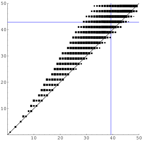
Figure 2 shows the observed distribution of $X:=2n-1-|S+S|$ (that is, the number of missing sums) for three million randomly generated subsets of $\{0,1,2,\dots,999\}$ . For example, the histogram shows that approximately 1.4% of these subsets $S$ have the largest possible sumset $S+S=\{0,\dots,1998\}$ , approximately 2.1% of them have exactly one element of $\{0,\dots,1998\}$ missing from their sumsets, and so on. The histogram is essentially identical to one generated from the complete data set for subsets of $\{0,\dots,26\}$ .

Notice that there is a “divot” at the top of the histogram: the observed frequencies of sets missing exactly 6 or 8 sums are both larger than the observed frequency of sets missing exactly 7 sums. In fact, the frequency for every even value seems to be larger than the average of its two neighbors, while the opposite is true for the frequencies of the odd values; in other words, the piecewise linear graph that connected the points at the tops of the histogram’s bars would alternate between being convex and concave.

Recall that the missing sums are typically very near the edges of the interval of possible sums. In particular, the missing sums for a subset $S$ of $\{0,\dots,999\}$ tend to be near either 0 or 1998, and are therefore so far apart that their numbers are independent. Therefore the distribution shown in Figure 2 is the sum of two independent, identically distributed (by symmetry) random variables that count the number of missing sums near one end. This is also essentially the same distribution as the number $Y$ of missing sums in randomly chosen (infinite) subsets $A$ of the nonnegative integers $\{0,1,\dots\}$ . That is, if $Y_{1},Y_{2}$ are independent with the same distribution as $Y$ , then $X$ and $Y_{1}+Y_{2}$ have approximately the same distribution (for large $n$ ).

At first one might think, then, that the parity phenomenon in Figure 2 is caused by that distribution being the sum of two independent copies of a simpler distribution. However, in this latter distribution (the first histogram in Figure 3), the disparity between odd and even values is even more apparent.

Fortunately, the phenomenon here is easy to analyze: if 0 is not in our randomly chosen subset of $\{0,1,\dots\}$ , then there are automatically 2 missing sums, namely 0 and 1, and the rest of the random subset can be shifted downwards by 1 to find the distribution of other missing sums:

{\mathbb{P}}\left[Y=k\right]=\sum_{i=0}^{\lfloor k/2\rfloor}{\mathbb{P}}\left[Y=k-2i\mid\min A=0\right]2^{-i}.

In other words, there is a yet more fundamental distribution (the second histogram in Figure 3), given by the number of missing subsums in a randomly chosen subset of $\{0,1,\dots\}$ containing 0. For example, that histogram shows that if a subset $S$ of $\{0,1,\dots\}$ containing 0 is chosen at random, there is about a 23.6% chance that $S+S=\{0,1,\dots\}$ .

The parity discrepancy seems to be absent in this last distribution, suggesting that it should be the focus of further analysis; the two more complicated preceding distributions can be reconstructed from suitable manipulations of this most fundamental one. The histogram suggests the existence of a function $f(x)$ , smooth and decaying faster than exponentially, such that the probability of a randomly chosen subset of $\{0,1,\dots\}$ that contains 0 missing exactly $n$ subsums is $f(n)$ .

It would of course be interesting to do a similar empirical analysis for the distribution of the number of missing differences; perhaps their joint distribution could even be reduced to a simpler one using similar observations.

7 Conjectures and open problems

Figure 4: The probability of a random subset of

\{0,\dots,n-1\}

being sum-dominant (top graph), difference-dominant (middle graph), or sum-difference-balanced (bottom graph)

We have already conjectured, in Conjecture 2, that the limiting proportions of difference-dominant, sum-difference-balanced, and sum-dominant subsets of $\{0,1,2,\dots,n-1\}$ approach nonzero limits as $n$ tends to infinity. (As long as the limits do in fact exist, Theorem 1 shows that they are necessarily nonzero.) Figure 4 shows the observed proportions, for $n\leq 27$ , of the subsets of $\{0,1,2,\dots,n-1\}$ that are difference-dominant, sum-difference-balanced, and sum-dominant, respectively. Note particularly that each graph is monotonic in $n$ , supporting our conjecture that the limits exist. Using ten million randomly chosen subsets of $\{0,1,\dots,999\}$ , we estimate:

Conjecture 18.

Using the notation of Conjecture 2,

\rho_{-}\approx 0.93,\quad\rho_{+}\approx 0.00045,\quad\text{and }\rho_{=}\approx 0.07.

In fact the philosophy behind Theorem 1 suggests somewhat more: a typical subset of $\{0,1,2,\dots,n-1\}$ will achieve virtually all possible sums and differences, and the ones that aren’t achieved are due to the edges of the subset. Since a positive proportion of sets have any prescribed edges, we make the following conjecture. Define

\rho_{j,k}:=\lim_{n\to\infty}\big(2^{-n}\,\#\big\{S\subset\{0,1,2,\dots,n-1\}:\\ |S+S|=2n-1-j,\,|S-S|=2n-1-k\big\}\big),

(7)

assuming the limit exists. Since the different set $S-S$ is symmetric about 0 and thus always has odd cardinality, we never have $|S-S|=2n-1-k$ with $k$ odd. Therefore we conjecture:

Conjecture 19.

For any nonnegative integers $j$ and $k$ with $k$ even, the limiting proportion $\rho_{j,k}$ defined above in (7) exists and is positive; furthermore,

\sum_{j=0}^{\infty}\sum_{\begin{subarray}{c}k=0\\ k\text{ even}\end{subarray}}^{\infty}\rho_{j,k}=1.

Remark.

Given Theorem 3, it seems reasonable to conjecture also that

\sum_{j=0}^{\infty}\sum_{\begin{subarray}{c}k=0\\ k\text{ even}\end{subarray}}^{\infty}k\rho_{j,k}=6\quad\text{and}\quad\sum_{j=0}^{\infty}\sum_{\begin{subarray}{c}k=0\\ k\text{ even}\end{subarray}}^{\infty}j\rho_{j,k}=10.

For any particular pair $j,k$ , if a single finite configuration of edges could be found that omitted exactly $j$ possible sums and $k$ possible differences, the methods of this paper would then show that $\rho_{j,k}>0$ (technically, that the analogous expression with $\liminf_{n\to\infty}$ in place of $\lim_{n\to\infty}$ is positive).

The last remark suggests as well the following open problem, for which a simple proof might exist, though we have not been able to find one.

Conjecture 20.

For any nonnegative integers $j$ and $k$ with $k$ even, there exists a positive integer $n$ , and a set $S\subset\{0,1,2,\dots,n-1\}$ with $0\in S$ and $n-1\in S$ , such that $|S+S|=2n-1-j$ and $|S-S|=2n-1-k$ .

Hegarty points out that his methods from [2] can establish both Conjecture 19 and Conjecture 20 in the case $j\geq k/2$ .

We know [1, 3] that essentially all subsets of $\{0,1,2,\dots,n-1\}$ of cardinality $O(n^{1/4})$ are Sidon sets and hence difference-dominant sets. More generally, we can show (perhaps in a sequel paper) that if $m=o(n^{1/2})$ , then almost all subsets of $\{0,1,2,\dots,n-1\}$ of cardinality $m$ are difference-dominant sets.

This result may indicate the presence of a threshhold. Set $p_{n}$ to vary with $n$ , and define $n$ independent random variables $X_{i}$ , with $X_{i}=1$ with probability $p_{n}$ . This defines a random set $A:=\{i\in\{0,1,2,\dots,n-1\}\colon X_{i}=1\}$ . The observations above can then be rephrased in the following way: if $p_{n}=o(n^{-1/2})$ , then $A$ is a difference-dominant set with probability 1 (as $n\to\infty$ ). We showed in this article that if $p_{n}=1/2$ , then $A$ is a sum-dominant set with positive probability (as $n\to\infty$ ), and our result is easily extended to $p_{n}=c>0$ . An important unanswered question is “Which sequences $p_{n}$ generate a sum-dominant set with positive probability?” Perhaps our last conjecture captures the correct notion:

Conjecture 21.

For each $n\geq 1$ , let $X_{n,0},X_{n,1},\dots,X_{n,n-1}$ be independent identically distributed random variables, and set $A_{n}:=\{i\colon 0\leq i<n,X_{n,i}=1\}$ . If both $|A_{n}|\to\infty$ and $|A_{n}|/n\to 0$ with probability 1, then the probability that $A_{n}$ is difference-dominant also goes to 1.

References

[1] A. P. Godbole, S. Janson, Jr. Locantore, and R. Rapoport (1999) Random Sidon sequences. J. Number Theory 75 (1), pp. 7–22. External Links: ISSN 0022-314X, Review MR 2000c:11031 Cited by: §7.
[2] P. V. Hegarty Some explicit constructions of sets with more sums than differences. pp. preprint. Cited by: §5, §5, §7.
[3] M. Nathanson (2003) On the ubiquity of sidon sets. Note: arXiv:math.NT/0304496 Cited by: §7.
[4] M. Nathanson (2006) Problems in additive number theory, 1. Note: arXiv:math.NT/0604340 Cited by: §1, §1.
[5] M. Nathanson (2006) Sets with more sums than differences. Note: arXiv:math.NT/0608148 Cited by: §1, §1.
[6] V. P. Pigarev and G. A. Freĭman (1973) The relation between the invariants $R$ and $T$ . pp. 172–174 (Russian). External Links: Review MR 0434995 Cited by: §5.
[7] I. Z. Ruzsa (1992) On the number of sums and differences. Acta Math. Hungar. 59 (3-4), pp. 439–447. External Links: ISSN 0236-5294, Review MR 1171750 Cited by: §5.