A combinatorial description of knot Floer homologyThanks: CM was supported by a Clay Research Fellowship.Thanks: PSO was supported by NSF grant number DMS-0505811 and FRG-0244663
Abstract.
Given a grid presentation of a knot (or link) in the three-sphere, we describe a Heegaard diagram for the knot complement in which the Heegaard surface is a torus and all elementary domains are squares. Using this diagram, we obtain a purely combinatorial description of the knot Floer homology of .
1. Introduction
Heegaard Floer homology [24] is an invariant for three-manifolds, defined using holomorphic disks and Heegaard diagrams. In [23] and [27], this construction is extended to give an invariant, knot Floer homology , for null-homologous knots in a closed, oriented three-manifold. This construction is further generalized in [25] to the case of oriented links. The definition of all these invariants involves counts of holomorphic disks in the symmetric product of a Riemann surface, which makes them rather challenging to calculate.
In its most basic form, knot Floer homology is an invariant for knots , , which is a finite-dimensional bi-graded vector space over , i.e.
This invariant is related to the symmetrized Alexander polynomial by the formula
| (1) |
(cf. [23], [27]). The topological significance of this invariant is illustrated by the result that
where here denotes the Seifert genus of (cf. [22]), and also the fact that has rank one if and only if is fibered ([10] in the case where and [19] in general). The invariant is defined as a version of Lagrangian Floer homology [6] in a suitable symmetric product of a Heegaard surface.
Our aim here is to give a purely combinatorial presentation of knot Floer homology with coefficients in for knots in the three-sphere. Our description can be extended to describe link Floer homology, and also it can be extended to describe the “full knot filtration” (and in particular the concordance invariant [21]). However, in the interest of exposition, we limit ourselves in the introduction to the case of knot Floer homology, referring the interested reader to Section 3 for more general cases.
To explain our combinatorial description, it will be useful to have the following notions.
A planar grid diagram consists of a square grid on the the plane with cells, together with a collection of black and white dots on it, arranged so that:
- •
every row contains exactly one black dot and one white dot;
- •
every column contains exactly one black dot and one white dot;
- •
no cell contains more than one dot.
The number is called the grid number of
Given a planar grid diagram , we can place it in a standard position on the plane as follows: the bottom left corner is at the origin, each cell is a square of edge length one, and every dot is in the middle of the respective cell. We then construct a planar knot projection by drawing horizontal segments from the white to the black dot in each row, and vertical segments from the black to the white dot in each column. At every intersection point, we let the horizontal segment be the underpass and the vertical one the overpass. This produces a planar diagram for an oriented link in . We say that has a grid presentation given by Figure 1 shows a grid presentation of the trefoil, with

It is easy to see that every knot (or link) in the three-sphere can be presented by a planar grid diagram. In fact, grid presentations are equivalent to the arc presentations of knots, which first appeared in [1], the square bridge positions of knots of [15], and also to Legendrian realizations of knots, cf. [17]; they have enjoyed a considerable amount of attention over the years, see also [3], [4]. The minimum number for which a knot admits a grid presentation of grid number is called the arc index of .
We find it convenient to transfer our planar grid diagrams to the torus obtained by gluing the topmost segment to the bottom-most one, and the leftmost segment to the rightmost one. In the torus, our horizontal and vertical arcs become horizontal and vertical circles. The torus inherits its orientation from the plane. We call the resulting object a toroidal grid diagram, or simply a grid diagram, for .
Given a toroidal grid diagram, we associate to it a chain complex as follows. The generators of are indexed by one-to-one correspondences between the horizontal and vertical circles. More geometrically, we can think of these as -tuples of intersection points between the horizontal and vertical circles, with the property that no intersection point appears on more than one horizontal (or vertical) circle.
We now define functions and (the Alexander and Maslov gradings) as follows.
Let us define a function on lattice points to be minus one times the winding number of the knot projection around . (This is shown in Figure 2 for our trefoil example.) Each black or white dot in the diagram lies in a square. We thus obtain distinguished squares, and each of them has four corners. We denote the resulting collection of corners We set
| (2) |

Next, given a pair of generators and , and an embedded rectangle in whose edges are arcs in the horizontal and vertical circles, we say that connects to if and agree along all but two horizontal circles, if all four corners of are intersection points in , and indeed, if we traverse each horizontal boundary components of in the direction dictated by the orientation that inherits from , then the arc is oriented so as to go from a point in to the point in . Let denote the collection of rectangles connecting to .
It is easy to see that if , and if and differ along exactly two horizontal circles, then there are exactly two rectangles in ; otherwise , cf. Figure 3.
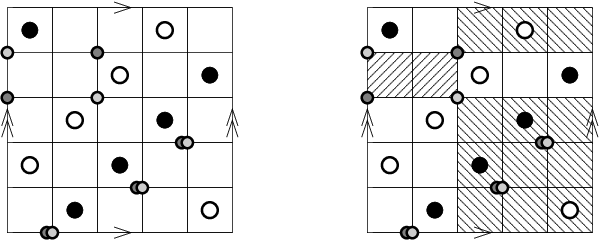
Given , it is easy to find an oriented, null-homologous curve composed of horizontal and vertical arcs, where each horizontal arc goes from a point in to a point in (and hence each vertical arc goes from a point in to a point in ). Now, suppose that is a two-chain whose boundary is a collection of horizontal and vertical arcs, and . We let and denote the number of white and black dots in respectively. Moreover, near each intersection point of the horizontal and vertical circles, has four local multiplicities. We define the local multiplicity of at , , to be the average of these four local multiplicities. Moreover, given , let
Now, is uniquely characterized up to an additive constant by the property that for each ,
| (3) |
where here is some two-chain whose boundary is . (Observe that we have displayed here a simple special case of Lipshitz’s formula for the Maslov index of a holomorphic disk in the symmetric product, cf. [14].) Note that the right-hand-side is independent of the choice of , as follows. Let and be the annuli given by and respectively. Note that any two choices of and connecting to differ by adding or subtracting a finite number of annuli and . But for each such annulus , , , and , and hence they do not change the right-hand-side. Moreover, the additive indeterminacy in is removed by the following convention. Consider the generator which occupies the lower left-hand corner of each square which contains a white dot, cf. Figure 4. We declare that .

Consider , the -vector space generated by elements of . We define a differential
by the formula
The condition that and is, of course, equivalent to the condition that the interior of the rectangle contains no black points, white points, or points amongst the and .
It is easy to see that drops Maslov grading by one and preserves Alexander grading. It is also elementary to verify that . Thus, we can take the homology of this complex to obtain a bigraded vector space over .
Let be the two-dimensional bigraded vector space spanned by one generator in bigrading and another in bigrading .
We can now state the following:
Theorem 1.1.
Fix a grid presentation of a knot , with grid number . Then, the homology of the above chain complex is isomorphic to the bigraded group .
The key point of the above theorem is to find a suitable Heegaard diagram for compatible with the knot . Indeed, the diagram we use has genus one, with Heegaard torus , and is represented as a collection of horizontal and vertical arcs. This Heegaard diagram has the property that the knot pierces in several pairs of points, and the very interesting property that the complement in of the attaching circles is a collection of squares. In this case, properties of the Maslov index ensure that the only holomorphic disks are rectangles. The chain complex we have described above, then, agrees with the Heegaard Floer complex for this diagram.
There are several other variants of Theorem 1.1. There is, for example, a version which calculates directly (though, of course, it is uniquely determined by the above result), except there one needs to consider a variant of the above the chain complex defined over a suitable polynomial algebra.
We also consider in this paper several other versions of Theorem 1.1. We discuss how to calculate the other variants of knot Floer homology, and also a variant for links.
This paper is organized as follows. In Section 2, we describe the construction of link Floer homology using Heegaard diagrams with the property that the link crosses the Heegaard surface in many points. This construction is then identified with the usual construction using methods from [25]. In Section 3, we identify the chain complex with the link Floer homology complex using the toroidal grid diagram of , interpreted as a Heegaard diagram for , and state some more general consequences. Finally, in Section 4, we describe some simple examples to illustrate our results.
Further remarks. Whereas the constructions in this paper give a purely combinatorial chain complex for knot Floer homology, Theorem 1.1 is still somewhat impractical, as the chain complex typically has far too many generators: for a knot with arc index , the procedure gives a chain complex with generators. It remains a very interesting challenge to come up with more efficient methods for calculating the homology of the complexes we describe here.
In a different direction, the relationship between our combinatorial description and Legendrian knots seems tantalizing: one wonders whether this is perhaps the hint of a connection with the holomorphic invariants of those objects, compare [2], [5], [18].
We would like to remind the reader that we have kept the introduction as elementary as possible. The more general results of Section 3 actually lead to a calculation of link Floer homology for links in . Also, the extra data about the “knot filtration” allows one to calculate the concordance invariant for knots. It is also the input needed to determine the ranks of Heegaard Floer homology groups of Dehn surgeries on a given knot , see [26].
Acknowledgements. This paper grew out of attempts at understanding an earlier preprint by the third author, who made the revolutionary observation that for Heegaard diagrams of a certain special form, the corresponding Heegaard Floer homology groups can be calculated combinatorially. In a different direction, that preprint also lead to the paper [29], which gives a method for describing of an arbitrary three-manifold in combinatorial terms.
We are grateful to Matthew Hedden, Mikhail Khovanov, John Morgan, and Lev Rozansky for their suggestions on an early version of our results. We are especially grateful to Dylan Thurston for his many interesting comments, especially for his suggestions for simplifying the Alexander gradings. Finally, we owe a great debt of gratitude to Zoltán Szabó, whose ideas have, of course, had a significant impact on this present work.
2. Link Floer homology with multiple basepoints
We review here the construction of knot and link Floer homology, considering the case where the link meets the Heegaard surface in extra intersection points. The fact that Heegaard Floer homology can be extracted from this picture follows essentially from [25].
Let be a Heegaard diagram, where is a surface of genus , is some positive integer, are pairwise disjoint, embedded curves in which span a half-dimensional subspace of (and hence specify a handlebody with boundary equal to ), is another collection of attaching circles specifying , and and are distinct marked points with
The data specifies a Heegaard splitting for some oriented three-manifold . In the present applications, we will be interested in the case where the ambient three-manifold is the three-sphere, and hence, we make this assumption hereafter.
Let resp. be the connected components of resp. .
We suppose that our basepoints are placed in such a manner that each component or contains exactly one basepoint amongst the and exactly one basepoint amongst the . We can label our basepoints so that contains and , and then contains and , for some permutation of .
In this case, the basepoints uniquely specify an oriented link in , by the following conventions. For each , let denote an arc in from to and let denote an arc in from to . Let be an arc obtained by pushing the interior of into , and be the arc obtained by pushing the interior of into . Now, we can let be the oriented link obtained as the sum
Definition 2.1.
In the above case, we say that is a -pointed Heegaard diagram compatible with the oriented link in .
Let denote the number of components of . Clearly, . In the case where , these are the Heegaard diagrams used in the definition of link Floer homology [25], see also [23], [27]. In the case where , these Heegaard diagrams can still be used to calculate link Floer homology, in a suitable sense.
Definition 2.2.
A periodic domain is a two-chain of the form
which has zero local multiplicity at all of the . A Heegaard diagram is said to be admissible if every non-trivial periodic domain has some positive local multiplicities and some negative local multiplicities.
Consider first the case where our link is in fact a knot. In this case, admissibility is automatically satisfied. Specifically, if we introduce cyclic orderings of and , and , so that and , then and . The condition that is a periodic domain ensures that for each , . Thus, if for some we have (i.e. ) then for some other , . Conversely, if for all , then there is some constant with all ; it follows readily that .
Let be a Heegaard diagram compatible with an oriented knot . We will consider Floer homology in the -fold symmetric product of the surface , relative to the pair of totally real submanifolds
| and |
Given , let denote the space of homology classes of Whitney disks from to , i.e. maps of the standard complex disk into which carry resp. to resp. , and points on the circle with negative resp. positive real part to resp. . (Note that when , homology classes of Whitney disks agree with homotopy classes.)
We consider now the chain complex over the polynomial algebra which is freely generated by intersection points between the tori and in . This module is endowed with the differential
| (4) |
where, as usual, denotes the space of homology classes of Whitney disks connecting to , denotes the moduli space of pseudo-holomorphic representatives of , denotes its formal dimension (Maslov index), denotes the local multiplicity of at the reference point (i.e. the algebraic intersection number of with the subvariety ), and denotes a count modulo two. As usual, in the definition of pseudo-holomorphic disks, one uses a suitable perturbation of the condition on the disk that it be holomorphic with respect to the complex structure on induced from some complex structure on , as explained in [24, Section ]; see also [7], [20], [8], [9] for more general discussions. We use here a sufficiently small perturbation to retain the property that if is pseudo-holomorphic, then for all , , cf. [24, Lemma ]. For the case where the Heegaard diagram is admissible, it is easy to see that Equation (4) gives a finite sum, compare [24].
The relative Alexander grading of two intersection points and is defined by the formula
| (5) |
where is any homotopy class from to . We find it convenient to remove the additive indeterminacy in : there is a unique choice with the property that
| (6) |
where is the symmetrized Alexander polynomial which could be made to work over by introducing signs. (These conventions are chosen to be consistent with those made in Proposition 2.3 below.)
Moreover, there is a relative Maslov grading, defined by
| (7) |
The relative Maslov grading can be lifted to an absolute grading using the observation that is a multiply-pointed Heegaard diagram for (a balanced -pointed Heegaard diagram in the terminology of [25]), and consequently, if one sets all the , the homology groups of the resulting complex, one obtains a relatively graded group which is isomorphic to (compare [25, Theorem ]). The Maslov grading is fixed by the requirement that
| (8) |
So far, we have made no reference to the basepoints , and indeed, the complex so far is the chain complex for for a multi-pointed Heegaard diagram, in the sense of [25, Section ].
This complex admits an Alexander filtration defined by the convention that any element has Alexander filtration level , and multiplication by the variables drops Alexander filtration by one, i.e.
Non-negativity of local multiplicities of pseudo-holomorphic disks ensures that this function indeed defines a filtration on the complex; i.e. we have an increasing sequence of subcomplexes indexed by integers , which are generated over by intersection points with .
In the case where , the above construction gives the chain homotopy type of the “knot filtration” on , called , which is a chain complex over the polynomial algebra . In this case, it was shown in [23] and [27] that the filtered chain homotopy type of the complex is a knot invariant. Our goal here is to show that this filtered chain homotopy type is also independent of .
In practice, it is often more convenient to consider the simpler complex generated by intersection points of and with coefficients in , endowed with the differential
For this complex, the function defines an Alexander grading which is preserved by the differential. One can think of as obtained from by first setting all the , and then taking the graded object associated to the Alexander filtration.
The following proposition shows how to extract the usual knot Floer homology from the above variants using multiple basepoints. The result is an adaptation of the results from [25, Section ], but we sketch the proof here for the reader’s convenience.
Proposition 2.3.
Let be a -pointed Heegaard diagram compatible with a knot . Then, the filtered chain homotopy type of , thought of as a complex over where can be any , agrees with the filtered chain homotopy type of . Moreover, we have an identification
| (9) |
where is the two-dimensional vector space spanned by two generators, one in bigrading , another in bigrading .
We first establish the following:
Lemma 2.4.
Let be an integer greater than one. After a series of isotopies, handleslides and stabilizations, any -pointed Heegaard diagram compatible with a knot , can be transformed into one with the following properties:
- •
there are curves and which bound disks and in
- •
contains the basepoint
- •
and meet transversally in a pair of points
- •
is disjoint from all with , and is disjoint from all with .
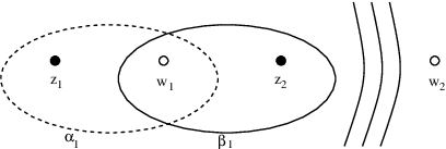
Proof.
Start from a pointed Heegaard diagram compatible with . Let be the component of which contains , and be the component of containing . In particular if are contained inside and respectively, then (since otherwise the basepoints and would determine a closed component of ; and since is a knot, we could conclude that ). After a sequence of handleslides amongst the and which do not cross any of the basepoints , , we can reduce to the case where and are both disks. Let and denote the boundaries of and respectively.
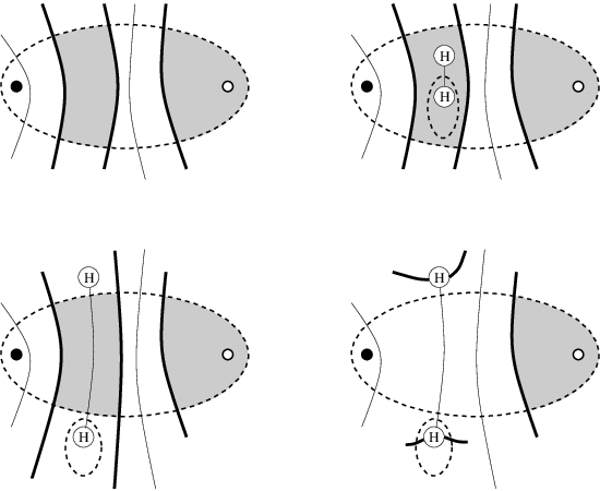
Note that, since and and , the intersection does not contain any . In fact, the various arcs divide into a collection of planar regions, one of which contains , another of which contains . All the other regions have no basepoints in them, and we call these unmarked regions. We can perform finger moves to eliminate all of the unmarked bigons in , by which we mean unmarked regions in whose closure meets in a single component in . Note that this might involve cancelling also intersection points betweeen with for some . (See Figure 6.) After doing this, consists of one region which is a bigon marked with , another which is a bigon marked with , and some unmarked regions which are all rectangles (i.e. their boundary meets in two components).

Now, consists of a bigon marked with and a (possibly empty) collection of unmarked rectangles. We can reduce the number of unmarked rectangular regions in by a stabilization, followed by four handleslides, as illustrated in Figure 7.
Finally, by performing handleslides of the additional and over and respectively (followed by some isotopies), we can arrange for the circles and to be disjoint from all the other and . ∎
Proof of Proposition 2.3. We use induction on . Obviously, in the case where , there is nothing to prove.
When using Lemma 2.4 we can reduce to the case where our diagram
has the special form in Figure 5. Note that under all the Heegaard moves used in Lemmaa 2.4, the filtered chain homotopy type of the associated chain complex remains invariant, as in [24], [23], [27].
We can de-stabilize the original diagram to get a -pointed Heegaard diagram
for the same knot. Let denote its corresponding filtered Heegaard Floer complex
thought of as a module over the polynomial algebra . It is generated by the corresponding intersection points of the tori and in .
The set of generators of the complex has the form , where and are the two points of intersection of and . Let be the subgroup of generated by intersection points of type and be the subgroup generated by those of type .
It is shown in the proof of [25, Proposition ] that for a suitable choice of complex structure on , the chain complex is identified with the mapping cone of the chain map
| (10) |
where the domain is identified with and the range with . Specifically, under the natural identifications of groups , , we have that the differential of is identified with the matrix
where here the variable corresponds to the basepoint which lies in the same -component as . In this mapping cone, the Alexander filtration of a generator in thought of as supported in is one higher than the Alexander filtration of the corresponding element, thought of as supported in .
Let us say a few more words about the identification of with the mapping cone used above, referring the interested reader to [25, Proposition ] for more details. Think of as formed by the connected sum of with a genus zero surface containing both and . Fixing conformal structures on and the sphere, we obtain a one-parameter family of conformal structures on by inserting a connected sum tube isometric to , and allowing to vary. When is sufficiently large, the chain complex can be identified with the mapping cone of
where is a map which counts points in a fibered product of moduli spaces of disks coming from and , fibered over a non-trivial symmetric product of the disk, where the maps are obtained as the preimage of the connected sum points and in and . (The term fits into this picture formally as the fibered product over the empty symmetric product.) To understand (and identify it with ), we must consider a second parameter in the space of conformal structures on , which is given by moving the connected sum point in . Indeed, it will be useful to move the connected sum point towards (so that as , limits onto ). In fact, for sufficiently close to (i.e. sufficiently large), the only non-empty moduli space which contributes to this fiber product consists of holomorphic disks in with Maslov index equal to two which carry some fixed point in the disk (whose distance to the -boundary of the disk goes to zero as ) into . When is sufficiently close to the -boundary, the count of these disks is identified with the count of Maslov index two -boundary degenerations for with local multiplicity at the connected sum point . Of course, the contribution of these boundary degenerations is given by multiplication by . This gives the identification of with the mapping cone of Equation (10). (Note that we broke the symmetry in the construction by moving towards rather than . If we moved towards instead, we would identify with the mapping cone of .)
For the second assertion of the proposition, view all the as being set to zero, and the above argument shows that
and hence a corresponding identification holds on the level of homology. Iterating this until we remain with two basepoints, we obtain the stated identification. ∎
It is perhaps more traditional to consider the filtration of (rather than ). This filtration is induced from the filtration of by setting . According to Proposition 2.3, this filtration is obtained as the induced filtration of .
2.1. Modifications for links
Recall that knot Floer homology has a generalization to the case of oriented links . For an -component, oriented link in the three-sphere, this takes the form of a multi-graded theory
where , with the latter isomorphism induced by an ordering of the link components. We sketch now the changes to be made to the above discussion for the purposes of understanding link Floer homology for Heegaard diagrams with extra basepoints, where by “extra” here we mean more than twice .
Suppose now that is a Heegaard diagram compatible with an oriented link in the sense of Definition 2.1.
We find it convenient to label the basepoints keeping track of which link component they belong to. Specifically, suppose is a link with components, and for , we choose basepoints to lie on the component. Letting be the index set of pairs with and . We now have basepoints and .
We can now form the chain complex defined over analogous to the version before, generated by intersection points of , with differential
This complex has a relative Maslov grading as before. It also has a relative Alexander grading which in this case is an -tuple of integers,
determined up to an overall additive constant by the formula
The indeterminacy in this case is a little more unpleasant to pin down (i.e. one must go beyond the multi-variable Alexander polynomial, which can be identically zero), but one can do this with the help of Proposition 2.5.
The complex inherits an Alexander filtration induced by the Alexander multi-grading of , and the convention that drops the multi-grading by the basis vector. In the case where , the filtered chain homotopy type of was shown to be a link invariant in [25]; it is the link filtration .
The analogue of can be defined as well: it is generated by intersection points of and over , endowed with the differential
This differential drops Maslov grading by one and preserves the Alexander multi-grading, and hence the homology groups inherit a Maslov grading and an Alexander multi-grading.
Proposition 2.5.
Let be a -pointed admissible Heegaard diagram compatible with an oriented link , with pairs of basepoints corresponding to the component of . Then, there is a filtered chain homotopy equivalence with the usual link filtration , viewed as a chain complex over . Moreover, there are (relative) multi-graded identifications
where is the two-dimensional vector space spanned by one generator in Maslov and Alexander gradings zero, and another in Maslov grading and Alexander grading corresponding to minus the basis vector.
3. Proof of Theorem 1.1 and its generalizations
The alert reader will have noticed by now that the toroidal grid diagrams from the introduction are a special case of the multiply-pointed Heegaard diagrams from Section 2. The Heegaard surface is the torus , the -circles are the horizontal circles, and the -circles are the vertical ones. The basepoints are the white dots, and are the black ones. Since for each and , and intersect in the single point , we see that the generators are, of course, the intersection points of with in . In our coordinate system, these generators can be thought of as graphs of permutations on letters. To apply the results from Section 2, we must verify the following:
Lemma 3.1.
Proof.
Let denote the Alexander grading of generators specified by the Heegaard diagram, and let denote the function defined in the introduction. Our aim is to show that .
Recall that the Alexander grading is determined up to an overall additive constant by the formula
where is any homology class connecting to . The right-hand side of this equation can be interpreted as the oriented intersection number of the knot with the two-chain associated to ; or alternatively as the linking number of with (which we think of now as an embedded curve in the three-sphere supported near its Heegaard torus). We can also think of this linking number as the intersection number of a Seifert surface for with . Deforming (without changing its intersection number with the Seifert surface for ) so that the horizontal segments are far under the Heegaard surface, and the vertical ones are far above it (so that each is the projection of an arc in which points vertically downwards, while each is the projection of an arc in which points vertically upwards), we can arrange that all the intersection points of with the Seifert surface occur in the arcs over and . Thus, we have established that for any two generators ,
| (11) |
or equivalently, that there is some with the property that for any generator , .
The proof that is elementary, albeit tedious. We sketch it here, leaving the details as an exercise for the interested reader; compare also [16]. One first checks that is a knot invariant, by verifying that it is unchanged by vertical and horizontal rotations of the toroidal grid diagram, as well as by the Reidemeister moves from [4] (see also [3]), which relate any two planar grid diagrams of the same knot. Then it suffices to show that the rational function of determined by the expression
which we know is , is actually a symmetric Laurent polynomial in . This can be done, for example, by verifying that it agrees with the symmetrized Alexander polynomial modulo two, using the skein relation:
The skein relation for can be readily verified by realizing the skein moves in grid position. Finally, a straightforward calculation in a diagram shows that when is the unknot. It follows that is the symmetrized Alexander polynomial modulo two, and in particular that is symmetric.
∎
Lemma 3.2.
Proof.
For we claim that its Maslov index is given by the formula
| (12) |
This is a particular case of Lipshitz’s formula for the Maslov index in an arbitrary Heegaard diagram [14]. However, for domains on a grid diagram, we can also give an elementary proof as follows.
Let denote the quantity on the right-hand side of Equation (12). First, note that when the domain associated to a homology class is a rectangle in the torus which contains none of the components of in its interior; in this case we also have because the moduli space of complex structures on a disk with four marked points on the boundary is one-dimensional.
Next, consider the natural map given by juxtaposition of flow lines:
The Maslov index is additive under this operation, i.e. We claim that the same is true for Indeed, the relation
is equivalent to
| (13) |
Let us denote by small translates of the curve on the torus, in the four diagonal directions. As in the proof of Lemma 3.1, we deform these curves by pushing their horizontal arcs under the Heegaard surface and their vertical arcs above the Heegaard surface; thus we can think of them as embedded curves in the three-sphere. The left-hand side of Equation (13) is then the average of the intersection numbers of the surface with each of Alternatively, it can be viewed as the average linking number of with these four curves. The right-hand side of (13) has a similar interpretation. Since the linking number is symmetric, the two sides are equal. Therefore, is additive under juxtaposition of flow lines.
Now, given an arbitrary pair , it is easy to construct a sequence of generators with , , and with the property that is a rectangle with no components of in its interior. It follows that if we let , then . The alpha curves cut the torus into annuli , and similarly the beta curves cut it into annuli . The homology classes and differ by adding or subtracting some number of copies of annuli or (thought of as elements of ), for which (because can be decomposed as a juxtapositon of two rectangles). It follows that .
We have verified Equation (12). It follows now that the relative Maslov grading from Equation (7) specializes to Equation (3).

We can lift from the relative to the absolute Maslov grading by performing handleslides on the -circles in our diagram which now are allowed to cross the , to reduce to a diagram which has intersection points in , and for which all the differentials in the chain complex vanish; indeed, it is identified with the homology of an -dimensional torus. The handleslides are performed by successively handlesliding over for , as pictured in Figure 8. It is easy to see now that the generator from the introduction can be connected to the bottom-most generator of the new chain complex by a collection of (Maslov index zero) triangles. According to (8), the grading of should be ∎
We can now turn to the following:
Proof of Theorem 1.1. The fact that the Alexander and Maslov gradings are identified has been verified in Lemmas 3.2 and 3.1 above. It remains to identify the differentials.
The circles and cut up into squares with . According to [24, Proposition ], homology classes of Whitney disks are determined by their underlying two-chain
where here for some point . Indeed, if and correspond to permutations and , then these induced two-chains are the ones that satisfy the property for all that
To understand the differential, we must count holomorphic disks in with . First, we classify all non-negative homology classes with Maslov index one.
Let . First observe that if is on circles, then it is in fact on all the circles, and is generated by the annular regions cut out by the circles. Now, if such a thing happens then , and its Maslov index is even.
Thus we can assume that is non-zero on at least two circles (say and ) and similarly non-zero on at least two circles ( and ). It follows that there are permutations and such that
Since , equality must hold throughout. It follows that is non-zero precisely on and , and is one of the two rectangles with four vertices , , , and . Without loss of generality, assume and . Then and , and it agrees with on the rest of the values. Also for the Maslov index requirement, does not lie in the interior of for any other .
Thus, we have established that the only with non-negative local multiplicities and Maslov index equal to one are those whose underlying domain is a rectangle of the form with . Moreover, we claim that in this case, the number of pseudo-holomorphic representatives of is odd. In fact, this can be seen by elementary complex analysis, using a (classical) complex structure on the symmetric product of , where one shows that in fact the moduli space consists of a single representative. Indeed, for this choice, the moduli space can be seen to correspond to involutions of (with the complex structure it inherits from ) which switch opposite sides of the rectangle. It is a simple exercise in conformal geometry that for any rectangle, there is a unique such involution.
We have thus completed the verification that the complex from the introduction coincides with the Heegaard Floer complex in the notation of Section 2. Theorem 1.1 now follows directly from Proposition 2.3 (Equation (9)). ∎
3.1. Other variants
There are other variants of Theorem 1.1, which should be clear from the constructions thus far. We state several of them for completeness.
Label the white dots , and let denote the local multiplicity of at . Consider the chain complex over the algebra also generated by , endowed with the differential
thought of as a filtered chain complex where the filtration level of each generator is its Alexander grading, and multiplication by the variable drops filtration level by one.
Theorem 3.3.
Fix a grid presentation of a knot , with grid number . The filtered chain homotopy type of coincides with the filtered chain homotopy type of the knot filtration .
Proof.
Of course, the other filtrations and from [23] can be extracted from this information.
We call attention to another other construction, which gives a concordance invariant for knots [21], [27]. This is a homomorphism from the smooth concordance group of knots to the integers, which can be used to bound the four-ball genus of knots, giving an alternate proof of the theorem of Kronheimer and Mrowka [13] confirming Milnor’s conjecture for the unknotting numbers of torus knots. This feature underscores its similarity with Rasmussen’s concordance invariant [28] from Khovanov homology [12]. However, these two invariants are known to be linearly independent [11].
Recall that the filtration of induces also a filtration of . The concordance invariant is by definition the minimal with the property that the map
is non-trivial.
We have a corresponding chain complex ; i.e. whose differential is given by
This is equipped with subcomplexes , generated by elements with integral , and
Corollary 3.4.
The concordance invariant is the minimal for which the map induced on homology
is non-trivial.
Proof.
Theorem 3.3 actually gives an identification of the filtered chain homotopy type of with . The result then follows from the definition of . ∎
Consider now the case of link Floer homology. In order to use the Heegaard diagram associated to a grid diagram to calculate link Floer homology, we must verify that it is admissible.
Lemma 3.5.
The diagram is admissible.
Proof.
The formal differences span the space of periodic domains. Drawing as a square, with equally spaced vertical and horizontal circles, it follows that the total signed area of any periodic domain is zero. Clearly, a non-zero region with this property must have both positive and negative local multiplicities. ∎
For the case of links, we number our dots and where is the index set consisting of with and , and the dots and lie on the component of .
In this case, the Alexander grading is an -tuple of integers. It is uniquely characterized by the property that for , the component of the Alexander grading is the winding number of about the sum of the black dots in minus its winding number around . Again, this can be more succinctly recorded by placing (minus one times) a vector of winding numbers at each vertex, and defining as the sum of these local contributions at each intersection point in . This can then be renormalized to be symmetric.
Once again, we have the chain complex as defined in the introduction, which now inherits an -tuple of Alexander gradings and a single Maslov grading.
There is also a refinement, , which is freely generated by over , endowed with the differential
Theorem 3.6.
There are multi-graded identifications
where is the two-dimensional vector space spanned by two generators, one in zero Maslov and Alexander multigradings, and the other in Maslov grading negative one and Alexander multi-grading corresponding to minus the basis vector. More generally, the multi-filtered chain homotopy type of is identified with the multi-filtered chain homotopy type of .
4. Examples
We give a few elementary illustrations of our results.
4.1. Hopf link
Consider the grid presentation for the Hopf link with grid number shown in Figure 9.

The generators of the chain complex are in one-to-one correspondence with permutations of the set For conciseness, we write the generator consisting of the intersections of the th horizontal circle with the th vertical circle as
There are eight empty squares in the grid. Each of them produces differentials between generators that differ by a transposition, according to the recipe:
The result is that there are sixteen differentials in They connect twelve of the generators, as shown schematically in Figure 10. Each of the other twelve generators is not connected by differentials to any other generators. Therefore, the homology of our complex has total rank
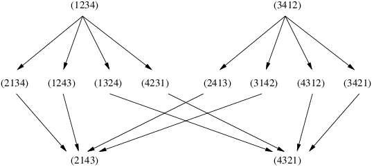
The Alexander bigrading of the generators is computed using the adaptation for links of Equation (2). For example,
To compute the Maslov gradings, we start with the canonical generator which has Then, we relate each of the other generators to the canonical one by a sequence of transpositions. Whenever two generators and differ by a transposition, if a two-chain has boundary then consists of two points and a rectangle, and it is straightforward to apply Equation (3). For example,
The result is that
Here, the notation denotes an upward shift in Alexander bigrading, i.e. if is a bigraded vector space, then
The link Floer homology of is cf. [25]. This confirms that
4.2. The trefoil
Consider the grid presentation of the trefoil knot shown in Section 1. There are, of course, generators of the chain complex. A quick glance at Figure 1 reveals 15 rectangles containing no black or white dot: fifteen , five , and five . Each rectangle gives rise to different differentials. With a little computer assistance or a great deal of patience, one finds that the homology of this complex has rank . Indeed, with the conventions used in Subsection 4.1, one finds that the generators correspond to permutations (listed in increasing Alexander grading):
These generators have Alexander gradings between and ; there are generators in gradings respectively. The knot Floer homology group for the left-handed trefoil is non-trivial in only three Alexander-Maslov bigradings , , and , and it has rank one in these three bigradings. Considering Maslov gradings as well, one immediately verifies that
References
- [1] H. Brunn. Über verknotete Kurven. Verhandlungen des Internationalen Math. Kongresses (Zurich 1897), pages 256–259, 1898.
- [2] Y. Chekanov. Differential algebra of Legendrian links. Invent. Math., 150(3):441–483, 2002.
- [3] P. R. Cromwell. Embedding knots and links in an open book. I. Basic properties. Topology Appl., 64(1):37–58, 1995.
- [4] I. Dynnikov. Arc-presentations of links: monotonic simplification. Fund. Math., 190:29–76, 2006.
- [5] Y. Eliashberg. Invariants in contact topology. In Proceedings of the International Congress of Mathematicians, Vol. II (Berlin, 1998), number Extra Vol. II, pages 327–338 (electronic), 1998.
- [6] A. Floer. Morse theory for Lagrangian intersections. J. Differential Geometry, 28:513–547, 1988.
- [7] A. Floer. The unregularized gradient flow of the symplectic action. Comm. Pure Appl. Math., 41(6):775–813, 1988.
- [8] A. Floer, H. Hofer, and D. Salamon. Transversality in elliptic Morse theory for the symplectic action. Duke Math. J, 80(1):251–29, 1995.
- [9] K. Fukaya, Y-G. Oh, K. Ono, and H. Ohta. Lagrangian intersection Floer theory—anomaly and obstruction. Kyoto University, 2000.
- [10] P. Ghiggini. Knot Floer homology detects genus-one fibred links. math.GT/0603445, 2006.
- [11] M. Hedden and P. Ording. The Ozsváth-Szabó and Rasmussen concordance invariants are not equal. math.GT/0512348, 2005.
- [12] M. Khovanov. A categorification of the Jones polynomial. Duke Math. J., 101(3):359–426, 2000.
- [13] P. B. Kronheimer and T. S. Mrowka. Gauge theory for embedded surfaces. I. Topology, 32(4):773–826, 1993.
- [14] R. Lipshitz. A cylindrical reformulation of Heegaard Floer homology. Geom. Topol., 10:955–1097 (electronic), 2006.
- [15] H. C. Lyon. Torus knots in the complements of links and surfaces. Michigan Math. J., 27(1):39–46, 1980.
- [16] C. Manolescu, P. S. Ozsváth, Z. Szabó, and D. P. Thurston. On combinatorial link Floer homology. math.GT/0610559.
- [17] H. Matsuda. Links in an open book decomposition and in the standard contact structure. Proc. of the Amer. Math. Soc., 2006.
- [18] L. Ng. Computable Legendrian invariants. Topology, 42(1):55–82, 2003.
- [19] Y. Ni. Knot Floer homology detects fibred knots. math.GT/0607156.
- [20] Y-G. Oh. On the structure of pseudo-holomorphic discs with totally real boundary conditions. J. Geom. Anal., 7(2):305–327, 1997.
- [21] P. S. Ozsváth and Z. Szabó. Knot Floer homology and the four-ball genus. Geom. Topol., 7:615–639, 2003.
- [22] P. S. Ozsváth and Z. Szabó. Holomorphic disks and genus bounds. Geom. Topol., 8:311–334, 2004.
- [23] P. S. Ozsváth and Z. Szabó. Holomorphic disks and knot invariants. Adv. Math., 186(1):58–116, 2004.
- [24] P. S. Ozsváth and Z. Szabó. Holomorphic disks and topological invariants for closed three-manifolds. Ann. of Math. (2), 159(3):1027–1158, 2004.
- [25] P. S. Ozsváth and Z. Szabó. Holomorphic disks, link invariants, and the multi-variable Alexander polynomial. math.GT/0512286, 2005.
- [26] P. S. Ozsváth and Z. Szabó. Knot Floer homology and rational surgeries. math.GT/0504404, 2005.
- [27] J. A. Rasmussen. Floer homology and knot complements. PhD thesis, Harvard University, 2003.
- [28] J. A. Rasmussen. Khovanov homology and the slice genus. math.GT/0402131, 2004.
- [29] S. Sarkar and J. Wang. A combinatorial description of some Heegaard Floer homologies. Preprint., 2006.