ORBIFOLD COHOMOLOGY OF HYPERTORIC VARIETIES
Abstract.
Hypertoric varieties are hyperkähler analogues of toric varieties, and are constructed as abelian hyperkähler quotients of a quaternionic affine space. Just as symplectic toric orbifolds are determined by labelled polytopes, orbifold hypertoric varieties are intimately related to the combinatorics of hyperplane arrangements. By developing hyperkähler analogues of symplectic techniques developed by Goldin, Holm, and Knutson, we give an explicit combinatorial description of the Chen-Ruan orbifold cohomology of an orbifold hypertoric variety in terms of the combinatorial data of a rational cooriented weighted hyperplane arrangement . We detail several explicit examples, including some computations of orbifold Betti numbers (and Euler characteristics).
Key words and phrases:
hyperkähler quotients, hypertoric varieties, orbifolds, orbifold cohomology, hyperplane arrangements2000 Mathematics Subject Classification
53C26, 52C351. Introduction
The main result of this manuscript is an explicit combinatorial computation of the Chen-Ruan orbifold cohomology [3] of an orbifold hypertoric variety . Hypertoric varieties are hyperkähler analogues of toric varieties, and were first introduced by Bielawski and Dancer [1], and further studied by Konno [10], [11] and Hausel and Sturmfels [7], among others. Just as a symplectic toric orbifold is determined by a labelled polytope, the theory of orbifold hypertoric varieties is intimately related to the combinatorial data of a related rational cooriented hyperplane arrangement . Our description of is given purely in terms of this arrangement . The fact that these hypertoric varieties are constructed as hyperkähler quotients of a quaternionic affine space (via the hyperkähler analogue of the Delzant construction of Kähler toric varieties) is crucial to our techniques.
Hyperkähler quotients appear in many areas of mathematics. For instance, in representation theory, Nakajima’s quiver varieties give rise to geometric models of representations (see e.g. [13], [14], [15]). Furthermore, many moduli spaces appearing in physics, such as spaces of Yang-Mills instantons on -manifolds or the solutions to the Yang-Mills-Higgs equations on a Riemann surface, arise via hyperkähler quotient constructions. In each case, the study of topological invariants, such as cohomology rings or -theory, of these quotients are of interest. In the case of hypertoric varieties, there are also close connections between the (ordinary or Borel-equivariant) cohomology rings of the varieties and the combinatorial theory of the corresponding hyperplane arrangements [10], [11], [7], [6]. Generalizing known such results to the orbifold case is of current interest. For example, recent work of Proudfoot and Webster [16][Section 6] on the intersection cohomology of singular hypertoric varieties and the cohomology of their orbifold resolutions contains cohomological formulas which only apply in the unimodular case; it would be of interest to know whether there are orbifold versions of their statements.
In this paper, we focus on the combinatorics of the hyperplane arrangement associated to the Chen-Ruan orbifold cohomology of orbifold hypertoric varieties. Chen-Ruan orbifold cohomology rings were introduced in [3] as the degree piece of the Gromov-Witten theory of an orbifold, following work in physics [18]. This ring carries, in addition to the data of the usual singular cohomology ring of the underlying space, more delicate information (e.g. about the orbifold structure groups). Additively, is simply the usual singular cohomology of the inertia orbifold associated to ; the product structure, on the other hand, is much more subtle, incorporating the data of higher twisted sectors. In this manuscript, we provide an explicit presentation, via generators and relations, of this Chen-Ruan cohomology ring for a class of orbifold hypertoric varieties.
Our approach is to develop hyperkähler analogues of the symplectic-geometric techniques as introduced by Goldin, Holm, and Knutson in [5] to compute Chen-Ruan orbifold cohomology. As in their work, we take advantage of the fact that a hypertoric variety is by construction a global quotient of a manifold by a torus. We now briefly recall the main results of [5]. Let be a compact connected torus, let be a compact Hamiltonian -manifold moment map , and suppose that is a regular value of . Then the inclusion induces a natural ring11 1 In this paper, we take rational coefficients for all cohomology rings. homomorphism, often called the Kirwan map:
| (1.1) |
which is a surjection [9]. Here is by definition the symplectic quotient of at . The main result of [5] is an orbifold cohomology version of (1.1) for abelian symplectic quotients. In other words, they show that the inclusion induces a surjective ring map (the “orbifold Kirwan map”)
| (1.2) |
where the domain is a new ring which they define: it is the inertial cohomology ring of the -space . (Here it is nontrivial that is a ring homomorphism; the same subtlety also arises in the hyperkähler case.) Moreover, they give an explicit description of the kernel of . Their proof relies on symplectic-geometric properties of the fixed point sets for in abelian Hamiltonian spaces, as well as on the original Kirwan surjectivity result (1.1).
In this paper we prove a parallel story in the hypertoric setting. A direct hyperkähler analogue of (1.2) is nontrivial for several reasons, foremost among which is that it is not known whether the hyperkähler analogue of (1.1) is, in general, surjective. However, in the special case where is a smooth or orbifold hypertoric variety [11], [7], obtained as a hyperkähler quotient of , a hyperkähler analogue of (1.1) does hold, allowing us to obtain results in this setting. The other nontrivial issues are the non-compactness of the hypertoric varieties (in [5], all orbifolds are assumed compact) and the analysis of the hyperkähler-geometric properties of the fixed point sets for . We deal with these issues in Section 4 to obtain the following. Let denote the hyperkähler moment map on , and its hyperkähler quotient at a regular value as described in Section 2.
Theorem 1.1.
Let be an orbifold hypertoric variety . There is a surjective ring homomorphism
| (1.3) |
where is the subgroup of generated by finite stabilizers, is the -subring of the inertial cohomology ring , and is the Chen-Ruan cohomology of .
The point of Theorem 1.1 is that we can in principle compute the orbifold cohomology of the hypertoric variety as a quotient of by the kernel of (1.3). In the spirit of [10, 11, 7, 6], we give an explicit algorithm for computing both the domain and the ideal in terms of the combinatorics of a central rational cooriented weighted hyperplane arrangement along with a choice of simple affinization . This combinatorial data is obtained from the data of the -action on and an appropriate choice of level set of the hyperkähler moment map (explained in detail in Section 2). We now give a rough statement of our main theorem, which gives a flavor of the ingredients in the computation; the precise version is Theorem 5.1.
Theorem 1.2.
Let be an orbifold hypertoric variety. Let be a simple affine rational cooriented hyperplane arrangement with positive normal vectors associated to as described in Section 2. Then the Chen-Ruan cohomology of is given by
where
- •
is a finite subgroup of determined by linear independence relations among the , made precise in (5.7);
- •
is an ideal determined by -weight data coming from the action of on specified by , made precise in Proposition 5.3;
- •
is an ideal generated by linear relations coming from an exact sequence of Lie algebras given by the -action on specified by , made precise in (2.1);
- •
is determined by intersection data of the hyperplanes in , and made precise in Proposition 5.6.
In summary, this manuscript can be viewed in any of the following ways. First, it is an example of an explicit computation of the Chen-Ruan orbifold cohomology of hyperkähler quotients, and a further development, in the hyperkähler setting, of the definition and use of inertial cohomology as introduced in [5]. In particular, we note that our methods would also apply to any class of hyperkähler quotients for which there exists an appropriate analogue of the Kirwan surjection (1.1). Similarly, although in this manuscript we restrict our attention to coefficients for our cohomology rings, if a -coefficient analogue of the Kirwan surjection for orbifold hypertoric varieties is proven, then our methods will easily generalize to the setting of coefficients. Second, it is another exploration of the relationship between the geometry of hypertoric varieties and the combinatorics of hyperplane arrangements. Finally, it is the hyperkähler-geometric analogue of the algebraic-geometric description of the Chow ring of toric Deligne-Mumford stacks in [2].
In [8], Jiang and Tseng independently develop techniques for an algebraic-geometric version of these results by defining “hypertoric DM stacks” using extended stacky fans, following work of [2]. Their work applies to the sub-class of hypertoric varieties M obtained by hyperkähler quotients at regular values of the form . In this case, there is a simple affine hyperplane arrangement in determined by the data of a moment map for a residual torus action on ; the results of [8] are phrased in terms of this arrangement . Our results, on the other hand, apply to an orbifold hypertoric variety obtained as a quotient at any regular value . This is because we do not keep track of the hyperkähler structure of the quotient (which does depends on this choice of level set); the Chen-Ruan orbifold cohomology of the quotient turns out to be independent of this choice, i.e. is the same for any regular value. The main difference between the approach taken in this manuscript and [8] is that Jiang and Tseng begin with the data of a simple hyperplane arrangement and then directly construct the hypertoric DM stack associated to , which has coarse moduli space the corresponding orbifold hypertoric variety. As a result, they compute the product in the orbifold Chow ring entirely in terms of the quotient hypertoric variety. In contrast, our method is to work almost entirely “upstairs” on with a linear -action, before taking a hyperkähler quotient. This simplifies some computations (as in [5]) by allowing us to work with linear -representations, and carries the information of a family of hypertoric varieties at once.
Since orbifold Chen-Ruan cohomology reduces to ordinary cohomology when is smooth, both our work and that of [8] reduce to the description of given in [11] (see also [7]) in the case when is a smooth hypertoric variety. As Jiang and Tseng illustrate [8], this can be useful to show that the ordinary cohomology of a smooth hyperkähler crepant resolution of as constructed by Kronheimer [12] is isomorphic to the orbifold cohomology of , which can be computed using [4].
We now give a summary of the contents of the paper. In Section 2, we give a brief account of the construction of hypertoric varieties as a hyperkähler quotient, based on the data of a hyperplane arrangement. In Section 3, we briefly recall the definition of inertial cohomology given in [5]. Then in Section 4, we prove that there exists a surjection in inertial cohomology as in (1.2). We give a combinatorial description of the Chen-Ruan orbifold cohomology of a hypertoric variety, based on the data of the hyperplane arrangement , in Section 5. In Section 6, we work out in detail several explicit examples, including some computations of orbifold Betti numbers and orbifold Euler characteristics. The Appendix (Section 7) contains a detailed discussion of the isomorphism between inertial cohomology of a -space and the Chen-Ruan cohomology of the quotient (also discussed for the compact case in [5]), as well as a careful proof of the correspondence between Chen and Ruan’s definition of the obstruction bundle with that used in the algebraic geometry literature (e.g. [4, 2]).
2. Background: hypertoric varieties
We first briefly describe the construction of hypertoric varieties in order to set the notation and conventions to be used throughout the rest of the paper. We refer the reader to [1, 6, 7] for a more leisurely account.
We begin with the hyperkähler space , thought of as a holomorphic cotangent bundle This is a hyperkähler manifold with real symplectic form given by the identification with and the canonical holomorphic symplectic form on a cotangent bundle. The standard linear diagonal action of the compact torus on induces an action on the holomorphic cotangent bundle which is hyperhamiltonian [1]. We will refer to this action as the standard hyperhamiltonian action of on . The hyperkähler -moment map on is given as follows. Let be a dual basis to in , and let where the are the base variables and the are the fiber variables. We have
Let be a central rational cooriented weighted hyperplane arrangement in with positive normal vectors in . Here, “weighted” means that we do not require the to be primitive vectors. We now use this data to restrict the action to that of a subtorus. Let be a basis of . Define a linear map by Let where with inclusion This yields an exact sequence
| (2.1) |
which on the one hand exponentiates to an exact sequence
| (2.2) |
and on the other hand dualizes to the exact sequence
| (2.3) |
We will always assume that the set of integer vectors spans over , so that the kernel is connected; this assumption is also made in [7].
Now we restrict the -action on to the subtorus . Let as in (2.3). Then is the -weight defining the action of the subtorus on the -th coordinate of . Let denote the corresponding element in Since the action of on is given by the natural lift of that on , we have that for
| (2.4) |
The moment maps for the hyperhamiltonian -action on are given by composing with the linear projection Thus we obtain the formulas
| (2.5) |
We will assume throughout that
In order to specify the hyperkähler quotient, we now pick a regular value at which to reduce. Any element specifies an affinization of via the equations
where denotes the natural pairing of a vector space and its dual, and is a lift of , i.e. (A different choice of lift just translates the whole hyperplane arrangement by a constant.)
In particular, the choice of parameter corresponds to three separate choices of affinization of the central arrangement . Hence a hypertoric variety is determined by the combinatorial data of a central weighted arrangement and, additionally, choices of affinization of . However, in the case of our computation, this data can be simplified considerably. This is because a preimage of a regular value of is -equivariantly diffeomorphic to the preimage of any other regular value; this can be seen by an argument essentially equivalent to the proof of [6][Lemma 2.1]. Hence the Chen-Ruan cohomology of can be seen to be isomorphic to that of as will be discussed further in Remark 3.6. In other words, the Chen-Ruan cohomology of an orbifold hypertoric variety is determined by the original central arrangement , and is independent of these choices of affine structures given by regular values. In practice, however, it is useful to pick a convenient affinization with which to work. Namely, if is chosen such that the corresponding affinization of is simple22 2 A hyperplane arrangement is simple if any subset of hyperplanes intersect in codimension ., then is a regular value [1][Theorem 3.3]. Here, since the last two parameters are both , only the first factor gives rise to a nontrivial affinization of . We will denote by this simple affine rational cooriented weighted hyperplane arrangement obtained from the data of and an appropriate
3. Background: inertial cohomology
We begin with a brief account of inertial cohomology as developed in [5], which gives us a model for computing the orbifold cohomology of the hyperkähler quotients constructed in Section 2. Readers already familiar with the definition of orbifold cohomology in the sense of Chen and Ruan will find Section 3.1 straightforward, since the product on the inertial cohomology of a -space is defined precisely to mimic the Chen-Ruan product in the case that the quotient is an orbifold, where acts with finite stabilizers on . The contribution of [5] is to notice that in other cases of -spaces (such as Hamiltonian -spaces), the product on inertial cohomology can be described in terms of a (different) product defined in terms of fixed point data. This (different) product, which is easier to compute, is briefly recalled in Section 3.2; it will play a key role in our computation of the Chen-Ruan orbifold cohomology of hypertoric varieties.
3.1. Inertial cohomology and the product
Let be a stably complex -space. For any let denote the -fixed points. Since is abelian, each is also a -space.
Definition 3.1.
The inertial cohomology of the space is, as a -module, given by
| (3.1) |
where the sum indicates the grading, i.e. .
The grading on the left hand side is a real-valued grading defined in [17] which is obtained from the grading on the right hand side by a shift depending (in this case) on the -action; see [5][Section 3] for a detailed discussion.
Remark 3.2.
In the case of the orbifold hypertoric varieties under consideration in this paper, it will turn out that the grading is integral and always even.
Although the stably complex structure does not enter into the definition of the inertial cohomology as an additive group, it is an essential ingredient in the definition of its product structure, which we now discuss; first, however, we warn the reader that the definition of the product on , which we denote by is not necessary for understanding the statement of our main Theorem 1.1, but is necessary for the proof. We include a brief definition only for completeness, and refer the reader to [5][Section 3] for details.
To describe the product, we make use of the top Chern class of the “obstruction bundle”, which is a vector bundle over connected components of certain submanifolds of . More specifically, let , let be the subgroup they generate, and the submanifold of points fixed by . For any connected component of , the normal bundle of in is naturally equipped with an -action. We may decompose into isotypic components with respect to the -action:
where denotes the character group of .
Definition 3.3.
Let and . For any connected component of , we define the logweight of with respect to , denoted , to be the real number in such that .
Note that for any elements and for any connected component of , the sum must be , or .
Definition 3.4.
The obstruction bundle is a vector bundle over each component of specified by
where . We write to denote the union over all connected components. Note that the dimension may vary over components. The virtual fundamental class is given by
where is the -equivariant Euler class of , considered as an element of .
Now let for , and denote the natural inclusions. These induce pullbacks for and the pushforward . Let and be homogeneous classes in . Then we define the product , a homogeneous class in , to be
where the product on the right hand side is the usual product on . Extending linearly, the product is defined on any two classes .
Remark 3.5.
It follows immediately from the definition of the product that, for any subgroup of , there is a subring given by
We call this ring the -subring of .
Remark 3.6.
It is straightforward to show from the definition of that if are stably complex -spaces equipped with locally free -actions and there exists a -equivariant diffeomorphism then as graded rings. Together with the proof given in the Appendix that the inertial cohomology of is isomorphic to the Chen-Ruan cohomology of the quotient orbifold, this justifies the claim in Section 2, i.e. is indeed independent of the choice of regular value . In particular, we may restrict without loss of generality to the case .
3.2. The product on when is robustly equivariantly injective
In this section, we give a different description of the product which will be easier to use for our computations. The -space is robustly equivariantly injective if the natural inclusion induces an injection in equivariant cohomology
for all . When satisfies this property, the product structure on can be described in terms of fixed point data and the local structure of the -action near fixed points; see [5]. Robust equivariant injectivity is a strong condition: for instance, if acts locally freely on , then and certainly cannot be robustly equivariantly injective. On the other hand, Hamiltonian -spaces are an important source of examples of robustly equivariantly injective -spaces.
For any component of the fixed point set , acts on the normal bundle to . This representation splits into isotypic component under the action:
Let and be homogeneous classes in . Then and are classes in and , respectively. Both of these rings are identified naturally with . We define
where is the equivariant Euler class of , and all the products on the right hand side are computed using the usual product in . Note that the exponent is either 0 (if ) or 1 (otherwise). By taking a sum over the connected components and by extending linearly, this defines a new product, which we call the product, on the image of in When is robustly equivariantly injective, the map is injective, so the product uniquely defines a product on . By abuse of notation, we denote this product also as for
The crucial fact, proven in [5], is that these two product structures agree, i.e.
when is robustly equivariantly injective. Hence in the robustly equivariantly injective case we may, for the purposes of computation, work exclusively with the product. Note that equipped with the -action described in Section 2 is a Hamiltonian -space, and in particular it is robustly equivariantly injective. We use this in Sections 5 and 6 to simplify the combinatorics.
4. Surjection in inertial cohomology
Let be a hypertoric variety as constructed in Section 2. Let be the level set of the hyperkähler moment map such that In this section, we show that the map
| (4.1) |
induced by the inclusion is a surjective ring homomorphism. In the appendix we prove that the latter ring is isomorphic to the orbifold cohomology of as (graded) rings, thus completing the proof of Theorem 1.1. An explicit description of both the domain and the kernel of , provided in Section 5, will yield a combinatorial description of . For the rest of the section, we will be largely following the outline of the proof of the symplectic case in [5]. However, there are several new considerations in the hyperkähler case, which we will discuss as they arise.
We must first justify why the inertial cohomology of the level is defined. For this, it suffices to observe that the normal bundle to is trivial since is the preimage of a regular value of . Therefore, the complex bundle is a stabilization of , so is also a stably complex -space and is well-defined.
Now consider the individual maps on Borel-equivariant cohomology
| (4.2) |
induced by the inclusions . Then we define the map on inertial cohomology to be the direct sum of the , i.e.
| (4.3) |
This is a priori only a map of -modules, not necessarily a ring homomorphism. Indeed, given an inclusion of the -fixed point set of a Hamiltonian -space, the induced map on inertial cohomology does not, in general, preserve the product structure since the obstruction bundles are all trivial for . However, if a -equivariant inclusion behaves well with respect to the fixed point sets for all then the obstruction bundles from Definition 3.4 also behave well, and the induced map on is in fact a ring homomorphism. We quote the following [5][Proposition 5.1].
Proposition 4.1.
(Goldin-Holm-Knutson) Let be a stably complex -space. Let be a -invariant inclusion and suppose also that is transverse to any , Then the map induced by inclusion is a ring homomorphism.
Thus, in order to check that the map is a ring homomorphism, it suffices to check that the level set is transverse to any . We have the following general computation.
Lemma 4.2.
Let be a compact torus, and let be a hyperhamiltonian -space with moment map Assume is a regular value of , and let denote the level set Then is transverse to for any
Proof.
The statement holds trivially . We assume that and that is connected; otherwise, we do the argument component by component. Let and let denote the inclusion. Since is a fixed point set of a Hamiltonian -action with respect to each symplectic form , is itself a hyperhamiltonian -submanifold of , with moment map
Since is regular, the Lie algebra of the stabilizer of is . In order to prove the transversality, it suffices to prove that is surjective. Since is Kähler, and , is surjective onto for each , where is the -orbit through and its tangent space at . Moreover, since is hyperkähler, the three subspaces for are mutually orthogonal. In order to show that is surjective onto , it suffices to show that for Without loss of generality we take For any
Thus maps the span of the three subspaces surjectively onto . This implies the level set is transverse to . ∎
Proposition 4.3.
Let be a compact torus, and let be a hyperhamiltonian -space with moment map Assume is a regular value of , and let denote the level set Then the map on inertial cohomology induced by the inclusion
is a ring homomorphism.
In particular, in our case of hypertoric varieties, the map defined in (4.3) is a ring homomorphism. Now it remains to show that is surjective. To do this, we show that
| (4.4) |
is surjective for each . We begin with an analysis of these -fixed point sets . A direct calculation shows that
is a quaternionic affine subspace of , where and
| (4.5) |
In addition, is also a hyperhamiltonian -space with moment map given by where denotes the inclusion. This computation allows us to conclude that (4.4) is the ordinary Kirwan map for the hypertoric subvariety of . Since these maps are known to be surjective [11, 7], we have just proven the following.
Theorem 4.4.
Let be a hyperhamiltonian -space given by restriction of the standard hyperhamiltonian -action on , where the inclusion is determined as in Section . Then the map on inertial cohomology induced by the inclusion
is a surjective ring homomorphism.
Inertial cohomology is a direct sum over infinitely many elements so Theorem 4.4 is not at all amenable to computation. However, Theorem 4.4 can be substantially simplified for computational purposes (in particular, it can be made finite). We first establish some terminology. Suppose a torus acts on a space . Suppose and the stabilizer group is finite. Then we call a finite stabilizer group. Similarly, given a finite stabilizer group , we call any element a finite stabilizer (element). We let denote the subgroup in generated by finite stabilizers. In the case of a linear -action on , this is a finite subgroup of , since the -action is determined by a finite set of weights.
By Remark 3.5,
| (4.6) |
is a subring of . We call this the -subring. We now show that is still surjective when restricted to the -subring.
Theorem 4.5.
Let be a hyperhamiltonian -space given by restriction of the standard hyperhamiltonian -action on , where the inclusion is determined as in Section . Let be the subgroup in generated by finite stabilizers. Then the map on the -subrings of inertial cohomology induced by the inclusion
is a surjective ring homomorphism.
Proof.
Since the level set is the preimage of a regular value of , acts locally freely on . In particular, if Hence for the map is automatically . Hence does not contribute to the image of , and In particular, is still surjective. ∎
By Theorem 4.5, we may restrict our attention to the -subring and the restricted ring map The only remaining step to complete the proof of Theorem 1.1 is the isomorphism of the inertial cohomology of the level set with the Chen-Ruan cohomology of the quotient This would then imply that, in order to compute , it would suffice to compute the domain and kernel of . This explicit computation is done in Section 5. The isomorphism mentioned above, for a general stably complex -space with locally free -action, is discussed in the compact case in [5][Section 4]; we place a detailed proof and its connection to the obstruction bundle in the algebraic geometry literature in an Appendix (Section 7).
5. The combinatorial description of
We now come to the main result of this manuscript. Using the inertial cohomology surjectivity result of Section 4 and the identification of inertial cohomology with Chen-Ruan orbifold cohomology in Section 7, we give in this section an explicit description of the Chen-Ruan orbifold cohomology of hypertoric varieties in terms of the combinatorial data of the hyperplane arrangement . Here is a choice of simple affinization of the central arrangement determining the hyperhamiltonian -action on , as detailed in Section 2. We then work out several concrete examples in Section 6.
We begin by stating our main theorem; for this, we must first set some notation. Let be a simple rational cooriented weighted hyperplane arrangement. Suppose that such that is linearly independent in , where the are the integer normal vectors to the hyperplanes . Then
| (5.1) |
is a finite group. Let be the finite subgroup in generated by all such . For an element we define
| (5.2) |
Let We define the following subsets of
where is the logweight defined in Definition 3.3. Note that these sets partition the set of indices corresponding to lines with nontrivial action by and . With this notation in place, we may state our main theorem.
Theorem 5.1.
Let be a hyperhamiltonian -space given by restriction of the standard hyperhamiltonian -action on , where the inclusion is determined by the combinatorial data of as in Section . Let be a simple affinization of . Then for any regular value the Chen-Ruan orbifold cohomology of the hyperkähler quotient is given by
where the ideals are defined as follows. First,
where . Second,
Finally,
where denotes a (possibly empty) subset of .
The proof of Theorem 5.1 involves three steps. First, we must show that the subgroup generated by finite stabilizeres defined in Section 4 is indeed the group generated by the in (5.1) above. above. Second, we prove that the ideals above are exactly the relations which yield the inertial cohomology . Finally, we show that the ideal exactly corresponds to the kernel of the inertial Kirwan map .
We begin with the first step, i.e. a description of the finite stabilizer group associated to the given -action on . As a bonus, we also give an (easy to compute) description of the global orbifold structure groups that arise in the quotient hypertoric variety. Let , where the -action on is determined by . We have the following.
Proposition 5.2.
Let be a hyperhamiltonian -space given by restriction of the standard hyperhamiltonian -action on , where the inclusion is determined by the combinatorial data of as in Section 2. Let be the positive normal vectors defining the hyperplanes in and as in (2.3).
- (1)
A subgroup of is a finite stabilizer subgroup of a subvariety of if and only if it is of the form
(5.7) where is such that is linearly independent in . In particular, the subvariety has global orbifold structure group .
- (2)
The subgroup in (5.7) is isomorphic to
- (3)
Any finite stabilizer occurs in a for such that forms a basis of .
Proof.
We begin with a general computation. Let Recall that the action of the subtorus is given by composing the homomorphism
| (5.8) |
with the standard linear action of on . It is immediate that
| (5.9) |
Now define Then (5.9) becomes
| (5.10) |
In particular, is finite if and only if the set spans , or equivalently, the intersection By the exactness of the sequence (2.1), this is equivalent to the condition that is linearly independent in . Conversely, given a subset with linear independent, any such that for and or for will have stabilizer exactly Moreover, the argument above immediately implies that has global orbifold structure group . This proves the first claim.
To prove the second claim, we will produce a map from to , which we will show takes values in . For the remainder of this computation, we identify with by (2.1) and with . In this language, is in exactly when any representative of has the property that for all We begin by constructing the map . Let Since by assumption, there exist linear combinations
| (5.11) |
where and the second linear combination is unique. Let where
Then by construction represents an element in , and we define A different choice of -linear combination in (5.11) yields the same , so is well-defined. Furthermore, by definition, if is trivial in , so also factors through the quotient
The map preserves additive structures, hence is a homomorphism. Furthermore, is an injection since if then the coefficients in (5.11) are integers, and hence Finally, to see that is surjective, let be a representative for an element in , with coordinates for for Then has the property that so is surjective. Hence is an isomorphism, as desired.
Finally, since we always have
for any in order to identify the finite stabilizer elements in , it suffices to consider the minimal subsets such that or equivalently, maximal linearly independent sets i.e. bases of . This proves the final claim. ∎
Thus, in order to compute , it suffices to find the subsets in which form a basis of . We also note that the subvarieties map under the moment map for to the intersection of the hyperplanes , so can easily be identified in the combinatorial picture using .
We now proceed to the second step, i.e. we describe the product structure on .
Proposition 5.3.
Remark 5.4.
The grading is given by for all , and , as specified in the Appendix.
Proof.
Recall that the -subring is by definition given by
Since each -th graded piece is the -equivariant cohomology of a contractible space, it has a single generator as a -module. Let denote the element in which is equal to for each -graded piece with and which is equal to the generator in the -th graded piece. Then is generated as a -module by these . Hence in order to determine the multiplicative structure, it suffices to find the product relations among these generators . Also, by the exact sequence (2.1), we may identify
Since is robustly equivariantly injective, we may compute all products in terms of the product instead of the product, as was explained in Section 3.2. By our assumptions on , all the weights defining the action of on are non-zero, and hence the only -fixed point is the origin . The -weights of the action on the normal bundle to are the weights Since the weights come in pairs, the definition of the product yields
If , then either or and the corresponding exponent is 0. Suppose . We now take cases. Suppose that In this case, for either or , and the -th term in the product above is . Similar computations show that if then the -th term is equal to , and if then the -th term is . Finally, given the identification of with , a representative of is given by . ∎
The third and final step is to determine the kernel of the inertial Kirwan map . Since is a direct sum of maps for it suffices to compute the kernel of each separately.
Suppose Then, as observed in Section 4, is the Kirwan map in usual cohomology for the hyperkähler Delzant construction of an orbifold hypertoric variety. This map is known to be surjective and the kernel has been explicitly computed. We quote the following.
Theorem 5.5.
(Hausel-Sturmfels) Let be a hyperhamiltonian -space given by restriction of the standard linear hyperhamiltonian -action on , where the inclusion is determined by the combinatorial data of as in Section 2 and let be a simple affinization of . Then the ordinary cohomology ring of the orbifold hypertoric variety is given by
| (5.13) |
where denotes a subset of .
We will apply Theorem 5.5 to the hyperhamiltonian action of on for each Since the expression in (5.13) uses the combinatorial data of the hyperplane arrangement corresponding to this action, our first task will be to describe explicitly the arrangement for each in terms of the original . Since the -action is defined as a restriction of the original -action on , the action on is given by the composition
where is the inclusion coming from the original Delzant sequence (2.1), and is the natural projection to the subspace, given by A simple linear algebra argument together with the commuting diagram
| (5.14) |
(where the top exact sequence is that in (2.1), the right vertical arrow is the natural projection, and is the composition of with the natural projection) shows that the map fits into the exact sequence
| (5.15) |
From this sequence we will be able to deduce the structure of the arrangement We note, however, the sequence (5.15) is not necessarily a standard Delzant exact sequence as in Section 2. This is because it is possible to have for some whereas this does not occur for a standard Delzant construction. This poses no serious problems, as will be discussed in more detail later. The relevant combinatorial data must therefore be contained in the non-zero images, .
Using (5.15), we may now explicitly describe the hyperplane arrangement for . First, sits naturally in the dual of the Lie algebra which is a subspace of . Specifically, it is the annihilator of the -dimensional subspace Hence, up to an affine translation, it may be identified with the intersection
| (5.16) |
where is the hyperplane orthogonal to in the original hyperplane arrangement . Moreover, by analyzing the dimensions of -orbits in the subvariety , it is straightforward to see that the affine hyperplanes in are exactly given by the intersections
| (5.17) |
where such that
The only indices which give non-empty hyperplanes in are those for which Thus, in addition to the standard Delzant construction for with certain basis vectors mapping to the corresponding normal vector defining a hyperplane in , we have in this case also some extra basis elements corresponding to the for which This poses no problems, because any such extra indices correspond to a subtorus of acting standardly on a quaternionic affine space, the moment map for which has level sets precisely equal to group orbits and hence has trivial hyperkähler quotient. In particular, the addition of such extra indices leaves the corresponding hypertoric variety topologically unchanged, allowing us (with only slight modifications) to use the known theorems for hypertoric varieties built via a standard Delzant construction.
We have the following Proposition.
Proposition 5.6.
Let be a hyperhamiltonian -space given by restriction of the standard hyperhamiltonian -action on , where the inclusion is determined by the combinatorial data of as in Section 2, and let be a simple affinization of . Let . Then the ordinary cohomology of the hypertoric subvariety is given by
where
| (5.18) |
where denotes a (possibly empty) subset of , and
Proof.
We begin by observing that the domain of the map may also be identified as by (2.1).
A subtlety that arises here is the presence of global stabilizers for the -action on the subsets for a non-trivial finite stabilizer. Clearly, if , then by definition has some non-trivial global stabilizer . Hence the -action on is not effective and in particular does not arise from a standard Delzant construction (since any such is effective). However, since is finite, is again a torus of dimension , and the inclusion maps on the level of Lie algebras are identical. The same holds at the level of cohomology rings, and hence the computation with global finite stabilizer is identical to the computation in the usual hyperkähler Delzant construction. (Put another way, the essential data for the computation is in the maps on Lie algebras.)
Putting together the description given in (5.16) and (5.17) of the hyperplane arrangement associated to (5.15), Theorem 5.5, and the commutative diagram (5.14), we see that the kernel of is generated by the relations given in (5.18). Note that if such that then
so . Finally, we observe that if (for instance if is not a finite stabilizer) then since in this case This in particular implies that we must have which is implied by our convention that we can take in the relations above and hence The result follows. ∎
We may now prove our main theorem, which gives a full combinatorial description of the Chen-Ruan orbifold cohomology of the orbifold hypertoric variety .
Proof.
(Proof of Theorem 5.1) We will give a description of the Chen-Ruan orbifold cohomology of as a quotient of by the kernel of . From Proposition 5.3, we have already seen that can be written as
Thus it remains to describe each piece of the kernel, Proposition 5.6 implies that where is defined in (5.18) and is here considered as an ideal in . Note that is a subset of the -th graded piece .
This concludes the proof except for one subtlety: in Proposition 5.6 we described ideal generators for with respect to the standard ring structure of Borel-equivariant cohomology, whereas in Theorem 5.1 we present generators with respect to the (or equivalently ) product on . Thus, given generators in the standard product, it is not immediate that their union (multiplied by appropriate ) would yield ideal generators for in the product. However, the -graded piece is a subring of in the product, and multiplication in the product of elements in and agrees with the standard -module structure on in Borel-equivariant cohomology. Since Theorem 5.5 gives -module generators for each , the result follows. ∎
6. Examples
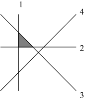
We compute several explicit examples in this section to illustrate our methods. Throughout, we identify Lie algebras with their dual spaces using the standard inner product. When illustrating the hyperplane arrangements, we will shade the intersection of the positive half-spaces corresponding to the cooriented hyperplanes.
6.1. A hyperkähler analogue of an orbifold
We begin with an example in which the corresponding Kähler toric variety is an orbifold . Let be the hyperplane arrangement depicted in Figure 6.1 and denote the corresponding hypertoric variety by . In this example, Here we will take the normal vectors to the hyperplanes to be primitive.

With respect to the standard bases in and , the map in (2.1) is given by
where the -th column is the vector normal to the -th hyperplane in Figure 6.1. By Proposition 5.2, the single orbifold point maps to the intersection of the hyperplanes and . The kernel of is given by the span of the single vector in . Hence the -action on with respect to which we take a hyperkähler quotient is induced by the linear action of on with weights on the three coordinates, respectively. In particular, it is immediate that the finite stabilizer subgroup is just . We compute the following table of logweights; the quantity is the degree of the corresponding generator as in (7.5).
| (6.1) |
Since there is only one non-trivial generator in as a -module, we only need to compute a single relation of the form (5.12), namely, the product of with itself. Since for we also have
as can be computed from the definitions (5), and so we have
The ideal of linear relations can be deduced from the matrix of to be
Finally, the ideal may be computed via the two pieces We have from Proposition 5.6 that
from which we conclude that
which is easily shown to be isomorphic to
where From this it is straightforward to compute that the orbifold Poincaré polynomial for is given by
so the orbifold Euler characteristic is .
Remark 6.1.
Let denote the hypertoric variety associated to the more general case in which (so the above case is ). The underlying Kähler toric variety is a weighted with a single orbifold point with orbifold structure group . An analogous computation yields the orbifold Poincaré polynomial
so has orbifold Euler characteristic .
6.2. A quotient of by a
We continue with an example in which the corresponding Kähler toric variety is a smooth , but now we add an extra hyperplane which introduces an orbifold point in the hypertoric variety. Let be the hyperplane arrangement depicted in Figure 6.2 and denote by the corresponding hypertoric variety. In this example, We take primitive normals to these hyperplanes.
The map is given by the matrix
By Proposition 5.2, the single orbifold point maps to the intersection of the hyperplanes and . The kernel of is given by the Lie subalgebra given by the span of the vectors and in . Therefore, the -action on with respect to which we take a hyperkähler quotient is given by
where and here we have chosen an identification of the kernel of with the standard -torus .
The finite stabilizer group may now be computed as follows. The weights for the -action are given by The only minimal spanning subset which leads to a non-trivial stabilizer is and the stabilizer subgroup is generated by the element Hence Then immediately and We will also use the following table.
| (6.2) |
As in the previous example, we only need to compute a single relation of the form (5.12), namely, the product of with itself. We have
and so
The ideal of linear relations is
Again as in the previous example, the ideal may be computed via the two pieces We have
We conclude
where
This simplifies to
Here, We see that the orbifold Poincaré polynomial is
so the orbifold Euler characteristic is .
7. Appendix: Inertial cohomology and Chen-Ruan cohomology
In this section, we show that there is a natural equivalence between the inertial cohomology of a stably complex space from Section 3 and the orbifold cohomology of when acts locally freely, i.e. that there exists a graded ring isomorphism
| (7.1) |
Applying this isomorphism to the case when is a level set of the hyperkähler moment map on and is an orbifold hypertoric variety completes the proof of Theorem 1.1. (There is a proof of a similar statement in [5], but here we drop their compactness assumption.) In addition, we show that the definition of the product structure for is also equivalent to another description used in the algebraic-geometry literature (e.g. [4], [2]).
We first prove (7.1) as additive groups. We simplify the presentation in [3] to the case when the group involved is abelian, and . Let , where is the local orbifold structure group at the point . We assume for simplicity that is connected (if not, take a direct sum over connected components). By definition,
| (7.2) |
where the degree shift is constant on connected components, and is defined below. Since in our case is a global quotient, each is a subgroup of and In other words, where and the -action is on the first coordinate. Notice that, for a given , . Since acts locally freely on , it certainly acts locally freely on . Therefore, (with coefficients) and
| (7.3) |
as additive groups. The right hand side of (7.3) is exactly the definition of , so we have proved the additive isomorphism (7.1).
We now prove that the isomorphism (7.1) also preserves the grading. The number appearing in (7.2) is obtained as follows; we assume At any point let be a representation specifying a local model at . Since is abelian, the image of is simultaneously diagonalizable; denote by the logweights of the eigenvalues of The sum
| (7.4) |
is well-defined, constant on connected components of , and gives the degree shift in [3] and (7.2).
We now show that this degree shift encoded by agrees with the degree shift in the definition of the grading for inertial cohomology in [5]. The local model can also be obtained by looking at the original -space . Namely, given a lift of the point is exactly and the representation above is given by the action of on the normal bundle in . Moreover, since acts trivially on , the only nontrivial eigenvalues of are those which occur in the representation of on a further quotient . In particular one may conclude that the sum (7.4) equals the sum
| (7.5) |
Even if is not compact, the grading shift is well defined (as long as is finite dimensional). In particular, the normal bundle does not degenerate as it goes out to infinity. This shows that the gradings agree.
We have left to show that the isomorphism (7.1) preserves the ring structure. The products on both and are defined using the notion of an obstruction bundle, so we begin by showing that the obstruction bundle of Definition 3.4, defined upstairs on , descends to the obstruction bundle of Chen and Ruan, defined on the quotient In their original paper [3], the authors define these bundles over -twisted sectors; however, their construction can be greatly simplified in the case of a global quotient so we restrict attention to this case below.
Chen and Ruan define their obstruction bundle using two ingredients; we describe each in turn. Consider a point and suppose that Let be the finite subgroup they generate. Let
Then there is a smooth map projecting to the first term. Let be the pullback of the tangent bundle; this is a complex -equivariant orbi-bundle over and is the first ingredient in the Chen-Ruan definition of the obstruction bundle.
The second ingredient involves only the subgroup . Let be a proper smooth Galois cover of branched over (for details see [4][Appendix]). The -action on induces an -action on , so we may define the topologically trivial -equivariant bundle with fiber over of complex rank , where the -action is only on the fiber. We denote this bundle by . Then the obstruction bundle of Chen and Ruan is given by the -invariant part of the tensor product of these two bundles, i.e.
| (7.6) |
We now wish to show that the obstruction bundle of Definition 3.4 descends to (7.6). As a first step, observe that is isomorphic to , so the base spaces of the two bundles certainly correspond. One reasonable way to lift the bundle might be to replace with in the Chen-Ruan definition. However, this tangent bundle is not complex. Since a fiber of the orbi-bundle can be constructed via -equivalence classes in , a natural idea would be to split at any point into the tangent directions along the orbits (which should not contribute), and its (complex) quotient bundle, . Alternatively, one can split into the tangent directions along the fixed point set, and its (complex) quotient . In either case, (or its quotient in ) does not contribute to the obstruction bundle, since
| (7.7) |
Thus only the normal bundle contributes, and we see that
| (7.8) |
quotients to . Note that is well-defined, even if is not compact. is a closed submanifold containing as a submanifold the orbit through ; thus is a quotient of a local model on of the representation downstairs.
It remains to show that the only -invariant subspaces of which contribute to (7.8) are the -isotypic components with We analyze each piece separately. We use Čech cohomology to compute with the , so let be an -invariant open cover of , i.e. for every there exists such that We denote this by for simplicity.
We claim that for the fiber is isomorphic as a -vector space to , where is the sheaf of -invariant sections of the topologically trivial -equivariant line bundle over . This can be seen at the level of cochains by the map
It is straightforward to check that is well-defined and an isomorphism using the definition of the -action on , which can be written, for ,
It may also be checked that commutes with the Čech differential, so as desired.
Furthermore, it is shown in [2] that The latter is -dimensional exactly when the sum inside is and -dimensional otherwise, so contributes nontrivially to if and only if As a bundle, each of these contributions is a line bundle over given as a sub-bundle of , since by construction is the trivial bundle over . We conclude that
where is the isotypic component of of weight .
Finally, under the isomorphism , the equivariant Euler class is mapped to the ordinary Euler class . The -product is then constructed to be identical to the definition given in [3]. We have proven (7.1), which we record as follows.
Theorem 7.1.
The inertial cohomology is isomorphic as a graded ring to the orbifold cohomology .
We now prove the correspondence of our definition of the obstruction bundle with a description in terms of right derived functors used in the algebraic geometry literature (e.g. [2], [4]). For this exercise, it is convenient to use the description in (7.8). In the algebraic-geometric context, the definition of the obstruction bundle (in the case of a global quotient by a locally free action) over is given as where are as above, is the projection, is the functor “pushforward and take -invariants”, and is its first right derived functor. By an argument similar to (7.7), only the normal bundle contributes nontrivially to this bundle, so We will work with this second description; in particular, we will show that in our (not necessarily algebraic) context, the right hand side of this equation is equal to our bundle (7.8).
We begin by computing . The sheaf of sections of is a -module, where is the sheaf of smooth functions on that are holomorphic restricted to any fiber of . By the push-pull formula,
Moreover, the pushforward sheaf can be described as
where here is the sheaf of smooth functions on and is the (usual) sheaf of holomorphic functions on . This implies that , so we finally have
as desired.
Acknowledgments
It is our pleasure to thank the American Institute of Mathematics for hosting a conference on the subject of Kirwan surjectivity, at which the authors began work on this project. We also thank Nicholas Proudfoot for useful conversations. The first author thanks Lisa Jeffrey and the University of Toronto for hospitality while some of this work was being conducted. The second author similarly thanks George Mason University. RG was partially supported by NSF-DMS Grant 0305128.
References
- [1] R. Bielawski and A. Dancer, The geometry and topology of toric hyperkähler manifolds, Comm. Anal. Geom., 8 (2000) 727–760.
- [2] L. A. Borisov, L. Chen, and G. G. Smith, The orbifold Chow ring of toric Deligne-Mumford stacks, J. Amer. Math. Soc., 18(1) (2005) 193–215 (electronic).
- [3] W. Chen and Y. Ruan, A new cohomology theory of orbifold, Comm. Math. Phys., 248(1) (2004) 1–31.
- [4] B. Fantechi and L. Göttsche, Orbifold cohomology for global quotients, Duke Math. J., 117(2) (2003) 197–227.
- [5] R. Goldin, T. S. Holm, and A. Knutson, Orbifold cohomology of torus quotients, Duke Math. J., 139(1) (2007), 89–139.
- [6] M. Harada and N. Proudfoot, Properties of the residual circle action on a hypertoric variety, Pacific J. Math., 214(2) (2004) 263–284.
- [7] T. Hausel and B. Sturmfels, Toric hyperkähler varieties, Doc. Math., 7 (2002) 495–534.
- [8] Y. Jiang and H.-H. Tseng, The Orbifold Chow Ring of Hypertoric Deligne-Mumford Stacks, arXiv:math.AG/0512199.
- [9] F. Kirwan, Cohomology of quotients in symplectic and algebraic geometry, (Princeton University Press, Princeton, N.J., 1984).
- [10] H. Konno, Equivariant cohomology rings of toric hyperkähler manifolds, Quaternionic structures in mathematics and physics (Rome), (1999) 231–240 (electronic).
- [11] H. Konno, Cohomology rings of toric hyperkähler manifolds, Int. J. of Math., 11(8) (2000) 1001–1026.
- [12] P. B. Kronheimer, The construction of ALE spaces as hyper-Kähler quotients, J. Differential Geom., 29(3) (1989) 665–683.
- [13] H. Nakajima, Instantons on ALE spaces, quiver varieties, and Kac-Moody algebras, Duke Math. J., 72(2) (1994) 365–416.
- [14] H. Nakajima, Quiver varieties and Kac-Moody algebras, Duke Math. J., 91(3) (1998) 515–560.
- [15] H. Nakajima, Quiver varieties and finite-dimensional representations of quantum affine algebras, J. Amer. Math. Soc., 14(1) (2001) 145–238 (electronic).
- [16] N. Proudfoot and B. Webster, Arithmetic and topology of hypertoric varieties, arXiv:math.AG/0411350.
- [17] Y. Ruan, Stringy orbifolds, in Orbifolds in mathematics and physics (Madison, WI, 2001), Contemp. Math., vol. 310 (Amer. Math. Soc., Providence, RI, 2002), pp. 259–299.
- [18] E. Zaslow, Solitons and helices: the search for a math-physics bridge, Comm. Math. Phys., 175(2) (1996) 337–375.