Predictability of the Burgers dynamics
under model uncertainty

Dirk Blömker Jinqiao Duan1. Institut für MathematikRWTH Aachen52062 Aachen, Germany2. Department of Applied MathematicsIllinois Institute of TechnologyChicago, IL 60616, USA

June 15, 2006

Abstract

Complex systems may be subject to various uncertainties. A great effort has been concentrated on predicting the dynamics under uncertainty in initial conditions. In the present work, we consider the well-known Burgers equation with random boundary forcing or with random body forcing. Our goal is to attempt to understand the stochastic Burgers dynamics by predicting or estimating the solution processes in various diagnostic metrics, such as mean length scale, correlation function and mean energy. First, for the linearized model, we observe that the important statistical quantities like mean energy or correlation functions are the same for the two types of random forcing, even though the solutions behave very differently. Second, for the full nonlinear model, we estimate the mean energy for various types of random body forcing, highlighting the different impact on the overall dynamics of space-time white noises, trace class white-in-time and colored-in-space noises, point noises, additive noises or multiplicative noises.

Key Words: Burgers equation with random boundary conditions, predictability, point forcing, boundary forcing, correlation function, mean energy, Itô’s formula, impact of noise.

Mathematics Subject Classifications (2000): 60H10,60H15, 35R60, 37H10

1 Introduction

The Burgers equation has been used as a simplified prototype model for hydrodynamics and infinite dimensional systems. It is often regarded as a one-dimensional Navier-Stokes equation. Our motivation for considering this equation comes from the modeling of the hydrodynamics and thermodynamics of the coupled atmosphere-ocean system. At the air-sea interface, the atmosphere and ocean interact through heat flux and freshwater flux with a fair amount of uncertainty [36, 19, 30]. These translate into random Neumann boundary conditions for temperature or salinity. The Dirichlet boundary condition is also appropriate under other physical situations. The fluctuating wind stress forcing corresponds to a random body forcing for the fluid velocity field. The coupled atmosphere-ocean system is quite complicated and numerical simulation is the usual approach at this time. In this paper, we consider a simplified model for this system, i.e., we consider the Burgers equation with random Neumann boundary conditions and random body forcing. Although the stochastic Burgers equation is widely studied, most work we know are for Dirichlet boundary conditions or periodic boundary conditions [18, 23, 11, 12]. The reference [37] studied the control of deterministic Burgers equation with Neumann boundary conditions.

We consider the stochastic Burgers equation with boundary forcing on the interval $[0,L]$

\partial_{t}u+u\cdot\partial_{x}u=\nu\partial_{x}^{2}u

(1)

\partial_{x}u(\cdot,0)=\alpha\eta\qquad\partial_{x}u(\cdot,L)=0.

(2)

Here $\alpha>0$ denotes the noise strength and $\eta$ is white noise, i.e., $\eta$ is a generalized Gaussian process with ${\mathbb{E}}\eta(t)=0$ and ${\mathbb{E}}\eta(t)\eta(s)=\delta(t-s)$ . The restriction to noise on the left boundary is only for simplicity. Analogous results will be true, if forces act on both sides of the domain.

We will see that boundary forcing coincides with point forcing at the boundary. Thus we also look at point forcing. As a simple example for point forcing, we consider

\partial_{t}v+v\cdot\partial_{x}v=\nu\partial_{x}^{2}v+\alpha\delta_{0}\eta

(3)

u(\cdot,-L)=u(\cdot,L)=0\;,

(4)

where $\delta_{0}$ is the Delta-distribution.

We will compare solutions of (1) and (3) with solutions of the stochastic Burgers equation with body forcing.

\partial_{t}v+v\cdot\partial_{x}v=\nu\partial_{x}^{2}v+\sigma\xi

(5)

either subject to Dirichlet or Neumann boundary conditions. Here the noise strength is denoted by $\sigma>0$ and $\xi$ is space-time white noise. I.e., $\xi$ is a generalized Gaussian process with ${\mathbb{E}}\xi(t,x)=0$ and ${\mathbb{E}}\xi(t,x)\xi(s,y)=\delta(t-s)\delta(x-y)$ . We will also consider trace class body noise, i.e., noise that is white in time but colored in space.

For the linearized equations, we will compare statistical quantities of both solutions, which are frequently used. One of them is the mean energy

\frac{1}{L}\int_{0}^{L}{\mathbb{E}}[u(t,x)-\overline{u}(t)]^{2}dx,

(6)

where

\overline{u}(t)=\frac{1}{L}\int_{0}^{L}u(t,x)dx.

Another important quantity, which gives information about the characteristic size of pattern, is the mean correlation function

C(t,r):=\frac{1}{L}\int_{0}^{L}{\mathbb{E}}[u(t,x)-\overline{u}(t)]\cdot[u(t,x+r)-\overline{u}(t)]dx,

(7)

which is usually averaged over all points $r$ with a given distance from $0$ . We obtain the averaged mean correlation function

\hat{C}(t,r)=\frac{1}{2}[C(t,r)+C(t,-r)]

(8)

where we employ the canonical odd and 2L-periodic extension of $u$ in order to define $C(t,r)$ for any $r\in{\mathbb{R}}$ .

For the linearized equation the main result states that mean energy and averaged mean correlation function are the same for solutions of (1) and (5). Nevertheless the solutions behave completely different. Furthermore, we give some qualitative properties like, for instance, the typical pattern size. This should carry over to a transient regime (i.e., small times) for the corresponding nonlinear equations.

For the full nonlinear Burgers model, we estimate the mean energy for various types of random body forcing, highlighting the different impact on the overall dynamics of space-time white noises, trace class white-in-time and colored-in-space noises, point noises, additive noises or multiplicative noises.

In the following, we discuss linear dynamics in §2 and nonlinear dynamics in §3.

2 Linear Theory

Define

A=\nu\partial_{x}^{2}

with

D(A)=\{w\in H^{2}([0,L])\ :\ \partial_{x}w(0)=0,\ \partial_{x}w(L)=0\}

It is well-known (cf. e.g. [13]) that $A$ has an orthonormal base of eigenfunctions $\{e_{k}\}_{k\in{\mathbb{N}}_{0}}$ in $L^{2}([0,L])$ with corresponding eigenvalues $\{\lambda_{k}\}_{k\in{\mathbb{N}}_{0}}$ . In our situation $e_{0}(x)=1/\sqrt{L}$ , $e_{k}(x)=\sqrt{2/L}\cdot\cos(\pi kx/L)$ for $k\in{\mathbb{N}}$ , and $\lambda_{k}=-\nu(k\pi/L)^{2}$ . Moreover $A$ generates an analytic semigroup $\{e^{tA}\}_{t\geq 0}.$ (cf. e.g. [31]).

In fact, $e^{tA}v_{0}$ is the solution of the following evolution problem

\partial_{t}v=Av,\qquad\partial_{x}v(\cdot,0)=\partial_{x}v(\cdot,L)=0,\qquad v(0,x)=v_{0}(x).

(9)

The solution is

e^{tA}v_{0}(x):=v(t,x)=\sum_{k=0}^{\infty}<v_{0},e_{k}>e^{\lambda_{k}t}e_{k},\quad t>0,\;0<x<L,

(10)

where $<\cdot,\cdot>$ is the usual scalar product in $L^{2}(0,L)$ .

We now consider the following linearized problems. First

\partial_{t}u=Au,\qquad\partial_{x}u(\cdot,0)=\alpha\partial_{t}\beta,\quad\partial_{x}u(\cdot,L)=0.

(11)

Here the white noise $\eta$ is given by the generalized derivative of a standard Brownian motion (cf. e.g. [1]), and $\alpha$ is the noise intensity.

Secondly,

\partial_{t}v=Av+\sigma\partial_{t}W,\qquad\partial_{x}v(\cdot,0)=0,\quad\partial_{x}v(\cdot,L)=0,

(12)

where the space-time white noise is given by the generalized derivative of an $Id$ -Wiener process. Namely, $W(t)=\sum_{k\in{\mathbb{N}}_{0}}\beta_{k}(t)e_{k}$ , where $\{\beta_{k}\}_{k\in{\mathbb{N}}}$ is a family of independent standard Brownian motions, and $\sigma$ is the noise intensity.

It is known (cf. e.g. [15]) that (12) has a unique weak solution given by the stochastic convolution (taking initial condition to be zero)

W_{A}(t)=\sigma\cdot\int_{0}^{t}e^{(t-\tau)A}dW(\tau)=\sigma\cdot\sum_{k\in{\mathbb{N}}_{0}}\int_{0}^{t}e^{(t-\tau)\lambda_{k}}d\beta_{k}(\tau)e_{k}.

(13)

We define the Neumann map ${\cal D}$ by

(1-A){\cal D}\gamma=0,\quad\partial_{x}{\cal D}\gamma(0)=\gamma,\ \partial_{x}{\cal D}\gamma(L)=0

for any $\gamma\in{\mathbb{R}}$ . It is known that ${\cal D}:{\mathbb{R}}\mapsto H^{2}([0,L])$ is a continuous linear operator. In fact, we have explicit expression for this linear operator

\displaystyle{\cal D}(\gamma)=\frac{e^{x}+e^{2L}e^{-x}}{1-e^{2L}}\gamma.

(14)

From [16] or [17] we immediately obtain, that (11) has a unique weak solution (taking initial condition to be zero)

Z(t)=(1-A)\int_{0}^{t}e^{(t-\tau)A}{\cal D}\alpha d\beta(\tau).

(15)

In the next section we derive explicit formulas for $Z$ in term of Fourier series.

2.1 Mean Energy

To obtain the Fourier series expansion for $Z,$ consider for $e\in D(A)$ and $\gamma\in{\mathbb{R}}$

$\displaystyle<{\cal D}(\gamma),(1-A)e>_{L^{2}([0,L])}$	$\displaystyle=$	$\displaystyle<{\cal D}(\gamma),e>-\int_{0}^{L}{\cal D}(\gamma)\cdot e_{xx}dx$	(16)
	$\displaystyle=$	$\displaystyle<{\cal D}(\gamma),e>-\int_{0}^{L}{\cal D}(\gamma)_{xx}\cdot edx+\left.{\cal D}(\gamma)_{x}\cdot e\right\|_{x=0}^{x=L}$
	$\displaystyle=$	$\displaystyle-\gamma e(0),$

by the definition of ${\cal D}$ . Hence,

$\displaystyle<Z(t),e_{k}>$	$\displaystyle=$	$\displaystyle<\int_{0}^{t}e^{(t-\tau)A}{\cal D}\alpha d\beta(\tau),(1-A)e_{k}>$	(17)
	$\displaystyle=$	$\displaystyle\int_{0}^{t}e^{(t-\tau)\lambda_{k}}<{\cal D}\alpha d\beta(\tau),(1-A)e_{k}>$
	$\displaystyle=$	$\displaystyle\alpha e_{k}(0)\cdot\int_{0}^{t}e^{(t-\tau)\lambda_{k}}d\beta(\tau).$

We now obtain

Z(t)=\alpha\cdot\sum_{k\in{\mathbb{N}}_{0}}e_{k}(0)\int_{0}^{t}e^{(t-\tau)\lambda_{k}}d\beta(\tau)e_{k}.

(18)

Finally,

Z(t)=\alpha e_{1}(0)\cdot\sum_{k\in{\mathbb{N}}}\int_{0}^{t}e^{(t-\tau)\lambda_{k}}d\beta(\tau)e_{k}+\alpha e^{2}_{0}(0)\beta(t)

(19)

and

W_{A}(t)=\sigma\cdot\sum_{k\in{\mathbb{N}}}\int_{0}^{t}e^{(t-\tau)\lambda_{k}}d\beta_{k}(\tau)e_{k}+\sigma\beta_{0}(t)\;.

(20)

If we now choose $\sigma=\alpha e_{1}(0)$ , we readily obtain that

{\mathbb{E}}\|Z(t)-\overline{Z}(t)\|^{2}=\sigma^{2}\cdot\sum_{k\in{\mathbb{N}}}\int_{0}^{t}e^{2\tau\lambda_{k}}d\tau={\mathbb{E}}\|W_{A}(t)-\overline{W_{A}}(t)\|^{2}\;,

where $\|\cdot\|$ is the norm in $L^{2}([0,T]).$ Hence, the mean energy in both cases is given by $\sigma^{2}L^{-1}\sum_{k\in{\mathbb{N}}}\int_{0}^{t}e^{2\tau\lambda_{k}}d\tau$ .

For the mean energy we can prove the following theorem, which is similar to the results of [4] and [5].

Theorem 1

Fix $\sigma^{2}=\alpha^{2}/L$ , then the mean energy $C_{Z}(t,0)=C_{W_{A}}(t,0)$ behaves like $C_{1}(\alpha^{2}/L)\sqrt{t/\nu}$ for $t\ll L^{2}/\nu$ , and like $C_{2}\alpha^{2}/\nu$ for $t\gg L^{2}/\nu$ .

The main difference to body forcing is the scaling in the length-scale $L$ . The long-time scaling is independent of $L$ , while the transient scaling is.

Figure 1: The scaling of the mean energy for boundary forcing.

2.2 Correlation Function

To obtain results for the correlation function, we think of $Z$ and $W_{A}$ to be periodic on $[-L,L]$ , and symmetric w.r.t. $0$ . I.e., we choose the standard $2L$ -periodic extension respecting the Neumann boundary conditions on $[0,L]$ . To be more precise, we extend $Z$ and $W_{A}$ in a Fourier series in the basis $e_{k}$ , which we then consider to be defined on whole ${\mathbb{R}}$ .

We consider firstly for $k,l\not=0$

\int_{0}^{L}e_{k}(x)e_{l}(x+r)dx=\left\{\begin{array}[]{ccc}Le_{k}(0)e_{l}(0)\frac{l((-1)^{k+l}-1)}{\pi(l^{2}-k^{2})}\sin(\pi lr/L)&:&k\not=l\\[2.84526pt] Le_{k}(0)^{2}\cos(\pi kr/L)&:&k=l\end{array}\right..

Now relying on the independence of the Brownian motions, it is straightforward to verify

	$\displaystyle C_{W_{A}}(t,r)$	$\displaystyle=$	$\displaystyle\frac{1}{L}{\mathbb{E}}<W_{A}(t,x)-\overline{W_{A}}(t),W_{A}(t,x+r)-\overline{W_{A}}(t)>$		(21)
		$\displaystyle=$	$\displaystyle\frac{\alpha^{2}e_{1}^{2}(0)}{L}\cdot\sum_{k\in{\mathbb{N}}}\int_{0}^{t}e^{2\tau\lambda_{k}}d\tau\cos(\pi kr/L)\;,$		(21)

as $\alpha^{2}e_{1}^{2}(0)=\sigma^{2}$ . Furthermore,

	$\displaystyle C_{Z}(t,r)$	$\displaystyle=$	$\displaystyle\frac{1}{L}{\mathbb{E}}<Z(t,x)-\overline{Z}(t),Z(t,x+r)-\overline{Z}(t)>$		(22)
		$\displaystyle=$	$\displaystyle C_{W_{A}}(t,r)+\frac{e_{1}^{2}(0)}{\pi}\sum_{k,l=1\atop k\not=l}^{\infty}\int_{0}^{t}e^{\tau(\lambda_{k}+\lambda_{l})}d\tau\frac{l((-1)^{k+l}-1)}{(l^{2}-k^{2})}\sin(\pi lr/L)\;.$		(22)

Obviously, $C_{Z}$ and $C_{W_{A}}$ do not coincide, but let us now look at the averaged correlation function

\hat{C}(t,r)=\frac{1}{2}[C(t,r)+C(t,-r)]\;.

Then it is obvious that

\hat{C}_{W_{A}}(t,r)=C_{W_{A}}(t,r)=\hat{C}_{Z}(t,r)\not=C_{Z}(t,r)\;.

(23)

Now

Theorem 2

For $\alpha^{2}e_{1}^{2}(0)=\sigma^{2}$ the mean energy and the averaged mean correlation functions $\hat{C}_{W_{A}}$ and $\hat{C}_{Z}$ for $Z$ and $W_{A}$ coincide for any $t\geq 0$ .

This is somewhat surprising, as realizations of $Z$ and $W_{A}$ behave completely different, when the condition $\alpha^{2}e_{1}^{2}(0)=\sigma^{2}$ is satisfied. See e.g. Figure 2 and Figure 3.

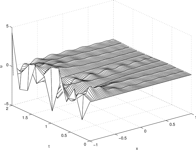
Refer to caption — Figure 2: *Random boundary condition*: One realization of the solution of the equation (11) for $L=1$ , $\nu=1$ , $\alpha=1$ and initial condition $u(x,0)=0$ .

It is even more surprising, as the scaling behavior of quantities like mean energy and mean correlation functions are an important tool in applied science, which for example is used to determine the size of characteristic length scales and the universality class the model belongs to. Here both linear models lie in the same class, although their behavior differs completely.

The scaling behavior with respect to $L$ and $t$ of the mean energy can be described using the results of [4], where the mean surface width for very general models was discussed. Therefore we focus on the scaling properties of the mean correlation function. Here we also want to investigate the dependence on $\alpha$ and $\nu$ .

First we consider the scaling properties of the correlation function $\hat{C}_{Z}(t,r)$ or $C_{W_{A}}$ , as given in (22). We are especially interested in the smallest zero of the function, which gives information about characteristic length scales or pattern sizes. For this, we use the normalized correlation function.

\rho_{Z}(t,r)=\frac{\hat{C}_{Z}(t,r)}{\hat{C}_{Z}(t,0)}.

(24)

Note that $C_{Z}(t,0)$ is the mean energy and the maximum of $r\mapsto\hat{C}_{Z}(t,r)$ .

We begin with some technical results. For any continuously differentiable and integrable function $f:{\mathbb{R}}^{+}\to{\mathbb{R}}$ we obtain using the mean value theorem

\left|\int_{0}^{\infty}f(x)dx-\sum_{k=1}^{\infty}f(k)\right|\leq\sum_{k=1}^{\infty}\sup_{\eta\in(k-1,k)}|f^{\prime}(\eta)|.

(25)

For $f(k):=e^{-2\tau\nu k^{2}\pi^{2}/L^{2}}\cos(k\pi r/L)$ it is easy to verify that

|f^{\prime}(k)|\leq e^{-\tau\nu k^{2}\pi^{2}/L^{2}}\cdot\frac{\pi}{L}\cdot\left[r+\frac{4\sqrt{\tau\nu}}{\sqrt{2e}}\right],

where we used that $x^{s}e^{-x^{2}\alpha}\leq(2\alpha e)^{-1/2}$ for any $x,\alpha\geq 0$ . Hence,

$\displaystyle\sum_{k=1}^{\infty}\sup_{\eta\in(k-1,k)}\|f^{\prime}(\eta)\|$	$\displaystyle\leq$	$\displaystyle\sum_{k=1}^{\infty}e^{-\tau\nu(k-1)^{2}\pi^{2}/L^{2}}\cdot\frac{\pi}{L}\cdot[r+\frac{4}{\sqrt{2e}}\sqrt{\tau\nu}]$	(26)
	$\displaystyle\leq$	$\displaystyle\frac{\pi}{L}[r+\frac{4}{\sqrt{2e}}\sqrt{\tau\nu}](1+\int_{0}^{\infty}e^{-\tau\nu k^{2}\pi^{2}/L^{2}}dk)$
	$\displaystyle=$	$\displaystyle\frac{\pi}{L}[r+\frac{4}{\sqrt{2e}}\sqrt{\tau\nu}](1+\frac{L}{\pi\sqrt{\tau\nu}}\cdot\int_{0}^{\infty}e^{-k^{2}}dk)$

and

\int_{0}^{t}\sum_{k=1}^{\infty}\sup_{\eta\in(k-1,k)}|f^{\prime}(\eta)|d\tau\leq C\frac{1}{L}\sqrt{\frac{t}{\nu}}[r+\sqrt{t\nu}][L+\sqrt{t\nu}].

(27)

Moreover,

	$\displaystyle\frac{1}{L}\int_{0}^{t}\int_{0}^{\infty}f(k)dkd\tau$	$\displaystyle=$	$\displaystyle\frac{1}{\pi}\int_{0}^{\infty}\frac{1-e^{-2t\nu k^{2}}}{2\nu k^{2}}\cos(kr)dk$		(28)
		$\displaystyle=$	$\displaystyle\frac{1}{\pi}\sqrt{\frac{t}{\nu}}\cdot G(\frac{r}{\sqrt{\nu t}}),$		(28)

with $G(x):=\int_{0}^{\infty}\frac{1-e^{-2k^{2}}}{2k^{2}}\cos(kx)dk$ .

Figure 4: A sketch of G

Using (23) we immediately obtain

C_{Z}(t,r)=\frac{\alpha^{2}}{L}\frac{1}{2\pi}\sqrt{\frac{t}{\nu}}\cdot G(\frac{r}{\sqrt{\nu t}})+{\cal O}\left(\frac{\alpha^{2}\sqrt{t}}{L^{3}\sqrt{\nu}}[r+\sqrt{t\nu}][L+\sqrt{t\nu}]\right)\;.

Note that the approximation with $G$ is not $L$ -periodic in $r$ , while $C_{Z}(t,r)$ is. The solution is that the error term is ${\cal O}(1)$ for $r$ near $L$ .

For the normalized correlation function we deduce

\rho_{Z}(t,r):=\frac{\hat{C}_{Z}(t,r)}{\hat{C}_{Z}(t,0)}=\frac{G(\frac{r}{\sqrt{\nu t}})+{\cal O}\left(\frac{1}{L^{2}}[r+\sqrt{t\nu}][L+\sqrt{t\nu}]\right)}{G(0)+{\cal O}\left(\frac{1}{L^{2}}[\sqrt{t\nu}][L+\sqrt{t\nu}]\right)}.

From the properties of $G$ we infer the following:

Theorem 3

Given $\delta\in(0,1)$ and sufficiently small $\epsilon_{2}>0,$ there exists some $\epsilon_{1}>0$ and three constants $0<C_{1}<C_{2}<C_{3}$ depending only on $\delta$ and $\epsilon_{2}$ such that for $t<\epsilon_{1}L^{2}/\nu$ the following holds:

\rho_{Z}(t,r)\geq\delta\quad\mathrm{\it for}\quad r\in[0,C_{1}\sqrt{t\nu}]

and

|\rho_{Z}(t,r)|<\epsilon_{2}\quad\mathrm{\it for}\quad r\in[C_{2}\sqrt{t\nu},C_{3}\sqrt{t\nu}].

Note that we did not show that the correlation function has a zero, but it is arbitrary small in a point $r_{\epsilon}\approx\sqrt{t\nu}$ . Therefor the theorem says that the typical length-scale is $\sqrt{t\nu}$ , at least for times $t\ll L^{2}/\nu$ .

For $t\to\infty$ we immediately obtain that

\hat{C}_{Z}(\infty,r)=\frac{\alpha^{2}}{\pi^{2}\nu}\sum_{k=1}^{\infty}\frac{1}{k^{2}}\cos(k\pi r/L)=:\frac{\alpha^{2}}{\nu}F(r/L)

and

|\hat{C}_{Z}(t,r)-\hat{C}_{Z}(\infty,r)|\leq\frac{\alpha^{2}}{\pi^{2}\nu}e^{-2t\nu\pi^{2}/L^{2}}\sum_{k=1}^{\infty}\frac{1}{k^{2}}.

Figure 5: A sketch of F

We can look for the explicit representation of $F$ , which is a $2$ -periodic function, and compute explicitly the zero, but all we need from $F$ is, that for a given small enough $\delta>0$ there is a $x_{\delta}>0$ such that $F>\delta$ on $[0,x_{\delta}]$ . Moreover, there is some $x_{0}$ such that $F(x_{0})=0$ .

Consider the normalized correlation function

\rho_{Z}(t,r)=\frac{\hat{C}_{Z}(t,r)}{\hat{C}_{Z}(t,0)}=\frac{F(r/L)+{\cal O}(e^{-2t\nu\pi^{2}/L^{2}})}{F(0)+{\cal O}(e^{-2t\nu\pi^{2}/L^{2}})}.

Assume that $t\nu\gg L^{2}$ (i.e., there is some small $\epsilon>0$ such that $\epsilon t\nu>L^{2}$ ). Now,

\rho_{Z}(t,x_{0}L)={\cal O}(e^{-2t\nu\pi^{2}/L^{2}})

and

\rho_{Z}(t,xL)\geq\frac{\delta}{F(0)}+{\cal O}(e^{-2t\nu\pi^{2}/L^{2}})>0

for any $x<x_{\delta}$ .

So for $t\gg L^{2}/\nu$ the first zero of $\rho_{Z}$ should be of order $L$ . A more precise formulation is:

Theorem 4

Given $\delta\in(0,0.8)$ and $\delta\gg\epsilon_{2}>0$ , there exists some $\epsilon_{1}>0$ , a constant $C>0$ , and a point $x_{o}>0$ depending only on $\delta$ and $\epsilon_{2}$ such that for $t>L^{2}/(\nu\epsilon_{1})$ we obtain the following:

\rho_{Z}(t,r)\geq\delta\quad\mathrm{\it for}\quad r\in[0,CL]

and

|\rho_{Z}(t,x_{0}L)|<\epsilon_{2}.

Thus the theorem tells us that for $t\gg L^{2}/\nu$ , the typical length scale is of order $L$ , which is the size of system. This result is true for both boundary and body forcing.

3 Nonlinear theory

For the nonlinear results we leave the setting of boundary forcing. Mainly, due to the lack of a-priori estimates. Usually, for Neumann boundary conditions one relies on the maximum principle to bound solutions, but the solution for boundary forcing is quite rough. Therefore, we hardly get useful results. Only, transient bounds for small times are possible to establish. For the next sections, we focus first on body forcing and later on point forcing. We will see later that boundary forcing is actually just a point forcing in a point at the boundary.

The main results of this sections are uniform bounds on the energy and thus on the correlation function $C$ , as $|C(t,r)|\leq C(t,0)$ , and $C(t,0)$ is the energy. Furthermore, we show that for $t\to 0$ the linear regime dominates. In [3] also H”older-continuity for the mean energy was shown for a quasigeostrophic model. We conclude this section by a qualitative discussion on upper bounds for the energy using additive and multiplicative trace-class noise.

3.1 Body forcing - Mean energy bounds

Here we provide bounds on the mean energy for the body forcing case. We consider additive space-time white noise case first, and show that the mean energy and thus the correlation function is uniformly bounded in time. This result is known (cf. [29]) for Burgers equation using the celebrated Cole-Hopf transformation, but we provide here a simple proof for completeness. Furthermore, our proof is based on energy estimates and it is easily adapted to other types of equations and additional terms in the equation. In contrast to that Cole-Hopf transformation is strictly limited to the standard Burgers equation.

For a long time for space-time white noise only uniform bounds for logarithmic moments were known. See [16, Lemma 14.4.1] or [14]. In [29] the transformation to a stochastic heat equation via the celebrated Cole-Hopf transformation was used to study finiteness of moments. Here we rely on a much simpler tool, which can also be applied to other equations. See for instance [3] for a quasigeostrophic model, where our analysis would apply, too.

Consider

\partial_{t}u+u\cdot\partial_{x}u=\nu\partial_{x}^{2}u+\sigma\partial_{t}W\;,

(29)

u(\cdot,-L)=u(\cdot,L)=0,\qquad u(x,0)=u_{0}(x).

(30)

Here $W$ is a $Q$ -Wiener process with a continuous operator $Q\in{\cal L}(L^{2})$ . Thus $W$ might be cylindrical, and we include the case of space-time white noise.

Using the semigroup $e^{t}A$ the solution for this system is (see [16] or [18]):

u(t)=e^{tA}u_{0}-\int_{0}^{t}e^{(t-\tau)A}(\lambda\Phi_{\lambda}(\tau)+\frac{1}{2}\partial_{x}u(\tau,x)^{2})d\tau+\Phi_{\lambda}(t)\;,

(31)

where for some $\lambda\geq 0$ fixed later

\Phi_{\lambda}(t)=\sigma\alpha\int_{0}^{t}e^{(t-\tau)(A-\lambda)}dW(\tau)

solves

\partial_{t}\Phi=\nu\partial_{x}^{2}\Phi-\lambda\Phi+\sigma\partial_{t}W

subject to

\Phi(\cdot,-L)=\Phi(\cdot,L)=0,\qquad\Phi(x,0)=0\;.

Our main result is now:

Theorem 5

Consider initial conditions $u_{0}$ with $E\|u_{0}\|^{2}<\infty$ , which are independent of the Wiener process $W$ (e.g. deterministic). Then the mean energy of the solution of (31) is uniformly bounded in time. I.e.,

\sup_{t\geq 0}{\mathbb{E}}\|u(t)-\overline{u}(t)\|^{2}<\infty\;.

Remark 1

Actually, we prove that $\sup_{t\geq 0}{\mathbb{E}}\|u(t)\|^{2}<\infty$ . The main problem in the proof is that after applying Gronwall-type estimates we end up with terms ${\mathbb{E}}\exp\{\int_{0}^{t}\|\Phi_{\lambda}(s)\|^{2}_{L^{\infty}}\}.$ This might blow up in finite time, as second order exponential moments of the Gaussian may fail to exist, if $t$ is too large. This is why we introduced artificially additional dissipation in the equation for $\Phi_{\lambda}$ , in order to get exponential moments small.

For the proof of Theorem 5 define

v(t)=u(t)-\Phi_{\lambda}(t)\quad\mathrm{for}\ t\geq 0,\ \lambda\geq 0\;.

(32)

We see that $v$ is a weak solution of

\partial_{t}v+\frac{1}{2}\partial_{x}(v+\Phi_{\lambda})^{2}=\nu\partial_{x}^{2}v+\lambda\Phi_{\lambda}

(33)

v(\cdot,-L)=v(\cdot,L)=0,\qquad v(x,0)=u_{0}(x).

(34)

The following calculation is now only formal, but it can easily made rigorous using for instance spectral Galerkin approximations. Taking the scalar product in (33) yields

$\displaystyle\frac{1}{2}\partial_{t}\\|v\\|^{2}$	$\displaystyle=$	$\displaystyle-\\|v_{x}\\|^{2}+\int_{-L}^{L}(v+\Phi_{\lambda})^{2}v_{x}\;dx+\int_{-L}^{L}\Phi_{\lambda}v\;dx$
	$\displaystyle\leq$	$\displaystyle-\\|v_{x}\\|^{2}+\\|\Phi_{\lambda}\\|_{H^{-1}}\\|v_{x}\\|+\|v_{x}\\|\\|\Phi_{\lambda}\\|^{2}_{L^{4}}+2\\|v_{x}\\|\\|\Phi_{\lambda}\\|_{L^{\infty}}\\|v\\|$
	$\displaystyle\leq$	$\displaystyle-\frac{1}{2}c_{p}^{2}\\|v\\|^{2}+4\\|v\\|^{2}\\|\Phi_{\lambda}\\|_{\infty}^{2}+2\lambda^{2}\\|\Phi_{\lambda}\\|_{L^{4}}^{4}+2\\|\Phi_{\lambda}\\|_{H^{-1}}^{2}\;,$

where we used Young inequality ( $ab\leq\frac{1}{8}a^{2}+2b^{2}$ ), and Poincare-inequality $\|v\|\leq c_{p}\|v_{x}\|$ . Now, from Gronwall-type inequalities

	$\displaystyle\\|v(t)\\|^{2}$	$\displaystyle\leq$	$\displaystyle e^{-c_{p}^{2}t+8\int_{0}^{t}\\|\Phi_{\lambda}\\|^{2}_{\infty}d\tau}\\|u(0)\\|^{2}$		(35)
			$\displaystyle+\int_{0}^{t}e^{-c_{p}^{2}(t-s)+8\int_{s}^{t}\\|\Phi_{\lambda}\\|_{\infty}^{2}d\tau}4(\lambda^{2}\\|\Phi_{\lambda}\\|_{L^{4}}^{4}+\\|\Phi_{\lambda}\\|_{H^{-1}}^{2})ds$		(35)

Now we use the following lemma, which is easily proved by Fernique’s theorem, if we consider $\Phi_{\lambda}$ as a Gaussian in $L^{2}([0,t_{0}],L^{\infty})$ .

Lemma 1

Fix $K>0$ and $t_{0}>0$ , then there is a $\lambda_{0}$ such that

\sup_{t\in[0,t_{0}]}{\mathbb{E}}\exp\{16\int_{0}^{t}\|\Phi_{\lambda}(s)\|^{2}_{L^{\infty}}ds\}\leq K^{2}

for all $\lambda\geq\lambda_{0}$ .

Furthermore, we use that all moments of $\|\Phi_{\lambda}\|_{L^{\infty}}$ and $\|\Phi_{\lambda}\|_{H^{-1}}$ are uniformly bounded in time. This is easily proven, using for instance the celebrated factorization method.

Now we first fix $K>0$ , and then $t_{0}$ such that $e^{-c_{p}^{2}t}K<\frac{1}{4}$ . This yields for $t\in[0,t_{0}]$ and $\lambda$ sufficiently large

{\mathbb{E}}\|v(t)\|^{2}\leq e^{-c_{p}^{2}t}K{\mathbb{E}}\|u(0)\|^{2}+4K\int_{0}^{t}e^{-c_{p}^{2}(t-s)}\Big({\mathbb{E}}(\lambda^{2}\|\Phi_{\lambda}\|_{L^{4}}^{4}+\|\Phi_{\lambda}\|_{H^{-1}}^{2})^{2}\Big)^{1/2}ds\;,

using Hölder, Lemma 1, and the independence of $u(0)$ from $\Phi_{\lambda}$ . We now find a constant $C$ depending on $t_{0}$ and $K$ such that

\sup_{t\in[0,t_{0}]}{\mathbb{E}}\|v(t)\|^{2}\leq K{\mathbb{E}}\|u(0)\|^{2}+C\qquad\mathrm{and}\qquad{\mathbb{E}}\|v(t_{0})\|^{2}\leq\frac{1}{4}{\mathbb{E}}\|u(0)\|^{2}+C

Using ${\mathbb{E}}\|u(t)\|^{2}\leq 2{\mathbb{E}}\|v(t)\|^{2}+2{\mathbb{E}}\|\Phi_{\lambda}(t)\|^{2}$ yields for a different constant $C$

\sup_{t\in[0,t_{0}]}{\mathbb{E}}\|u(t)\|^{2}\leq K{\mathbb{E}}\|u(0)\|^{2}+C\qquad\mathrm{and}\qquad{\mathbb{E}}\|u(t_{0})\|^{2}\leq\frac{1}{2}{\mathbb{E}}\|u(0)\|^{2}+C

Now we repeat the argument for $k\in\mathbb{N}$ by defining $v(t)=u(kt_{0}+t)-\tilde{\Phi}_{\lambda}(t)$ , where $\tilde{\Phi}_{\lambda}(t)$ has the same distribution than $\Phi_{\lambda}(t)$ due to a time shift of the Brownian motion. Now $v$ solves again (33) with initial condition $u(kt_{0})$ . Note that by construction $u(kt_{0})$ is independent of $\tilde{\Phi}_{\lambda}$ .

Repeating the arguments as before yields for $k\in\mathbb{N}_{0}$

\sup_{t\in[0,t_{0}]}{\mathbb{E}}\|u(t+kt_{0})\|^{2}\leq K{\mathbb{E}}\|u(kt_{0})\|^{2}+C

and

{\mathbb{E}}\|u((k+1)t_{0})\|^{2}\leq\frac{1}{2}{\mathbb{E}}\|u(kt_{0})\|^{2}+C\;.

Now the following lemma, which is a trivial statement on discrete dynamical systems, finishes the proof.

Lemma 2

Suppose for $q<1$ and some $C>0$ we have $a_{n+1}<qa_{n}+C$ , then $a_{n}$ is bounded by

a_{n}<\frac{C}{1-q}+a_{0}\;.

3.2 Point forcing - Mean energy bounds

Consider hyperviscous Burgers equation with point-forcing. We would like to proceed exactly the way, we did in the previous section, But we can not, as for point forcing, the solution of the linear equation might fail to be in $L^{\infty}$ . This is why we add additional damping. Hyperviscous Burgers equation has been studied in several occasions. See for example [7, 27, 32].

Consider for some $\epsilon>0$ the operator $A_{\epsilon}=-\nu(-\Delta)^{1+\epsilon}$ , where $\Delta$ is the Laplacian subject to Dirichlet boundary conditions. Then the hyperviscous Burgers equation is given by

\partial_{t}u+u\cdot\partial_{x}u=A_{\epsilon}u+\alpha\delta_{0}\dot{\beta}

(36)

u(\cdot,-L)=u(\cdot,L)=0,\qquad u(x,0)=u_{0}(x).

(37)

Here, $\beta$ is a standard Brownian motion and $\delta_{0}$ the Delta-distribution.

Using the semigroup $e^{tA_{\epsilon}}$ the solution for this system is (see [16] or [18]):

u(t)=e^{tA_{\epsilon}}u_{0}-\int_{0}^{t}e^{(t-\tau)A_{\epsilon}}(\lambda\Phi_{\lambda}(\tau)+\frac{1}{2}\partial_{x}u(\tau,x)^{2})d\tau+\Phi_{\lambda}(t)

(38)

where for some $\lambda\geq 0$ fixed later

\Phi_{\lambda}(t)=\alpha\int_{0}^{t}e^{(t-\tau)(A_{\epsilon}-\lambda)}\delta_{0}(x)d\beta(\tau)

solves

\partial_{t}\Phi=A_{\epsilon}\Phi-\lambda\Phi+\alpha\delta_{0}\dot{\beta}

subject to

\Phi(\cdot,-L)=\Phi(\cdot,L)=0,\qquad\Phi(x,0)=0\;.

Using the standard orthonormal basis $\{e_{k}\}_{k\in\mathbb{N}}$ of eigenfunctions of $A_{\epsilon}$ given by $e_{k}(x)=\sqrt{1/L}\cdot\sin(-L+\frac{\pi kx}{2L})$ with corresponding eigenvalues $\lambda_{k}=-(\pi k/2L)^{2+2\epsilon}$ , we see

\Phi_{\lambda}(t)=\alpha\sum_{k=1}^{\infty}\int_{0}^{t}e^{(t-\tau)(\lambda_{k}-\lambda)}d\beta(\tau)e_{k}(0)e_{k}\;.

(39)

Note that the Fourier-coefficients of that series are not at all independent. Thus we cannot rely on the better regularity results available for the stochastic convolution of the previous chapter. Especially, for $\epsilon=0$ we cannot show that $\Phi_{\lambda}(t)\in L^{\infty}([-L,L])$ .

Note that the series expansion of boundary and point forcing is very similar. Thus we can regard boundary forcing at a point forcing at the boundary, when the equation is subject to Neumann boundary conditions.

Our main result is now:

Theorem 6

For all $\epsilon>0$ and all initial conditions $u_{0}$ independent of $\beta$ with $E\|u_{0}\|^{2}<\infty$ the solution of (38) satisfies that the mean energy is uniformly bounded in time. I.e.,

\sup_{t\geq 0}{\mathbb{E}}\|u(t)-\overline{u}(t)\|^{2}<\infty\;.

We will proceed exactly as in the previous section. Now $v=u-\Phi_{\lambda}$ is a weak solution of

\partial_{t}v+\frac{1}{2}\partial_{x}(v+\Phi_{\lambda})^{2}=\nu\partial_{x}^{2}v+\lambda\Phi_{\lambda}\;,

(40)

again subject to Dirichlet boundary conditions and initial condition $v(0)=u_{0}.$

Now consider first the nonlinear term for some small $\delta>0$ . Using Hölder, Sobolev embedding of $H^{\frac{1}{2}-\frac{1}{p}}$ into $L^{p}$ and the bound

\|u\|_{H^{2\gamma}}\leq C\|A_{\epsilon}^{\gamma/(1+\epsilon)}u\|

yields

	$\displaystyle\int_{-L}^{L}v\Phi_{\lambda}v_{x}dx$	$\displaystyle\leq$	$\displaystyle\\|v\\|_{L^{2+\delta}}\\|\Phi_{\lambda}\\|_{L^{(4+2\delta)/\delta}}\\|v_{x}\\|$
		$\displaystyle\leq$	$\displaystyle C\\|A_{\epsilon}^{\frac{1}{4}\frac{1}{1+\epsilon}\frac{\delta}{2+\delta}}v\\|\\|\Phi_{\lambda}\\|_{L^{(4+2\delta)/\delta}}\\|A_{\epsilon}^{\frac{1}{2}\frac{1}{1+\epsilon}}v\\|\;,$

Now we can easily find an $\delta>0$ sufficiently small such that there is a $p=p(\epsilon)\in(2,\infty)$ such that (using interpolation inequality)

\int_{-L}^{L}v\Phi_{\lambda}v_{x}dx\leq C\|v\|_{L^{2}}\|\Phi_{\lambda}\|_{L^{p}}\|A_{\epsilon}^{\frac{1}{2}}v\|\;.

Now we can use the same proof as in the section before. We only need that $\Phi_{\lambda}(t)\in L^{\infty}(0,L)$ . To be more precise, an easy calculation using the series expansion of (39) shows that for any $\epsilon>0$

\sup_{t\geq 0}\mathbb{E}\|\Phi_{\lambda}(t)\|^{2}_{L^{\infty}}\leq C_{\epsilon}\sup_{t\geq 0}\mathbb{E}\|\Phi_{\lambda}(t)\|^{2}_{H^{\frac{1+\epsilon}{2}}}\to 0\quad\mathrm{as\ }\lambda\to\infty\;.

It is now straightforward to prove an analog to Lemma 1. The remainder of the proof is analogous to the section before.

Let us remark that we could even simplify that proof a little bit, by avoiding second order exponentials of $\Phi_{\lambda}$ . In that case we could work with $\lambda=0$

3.3 Body forcing - Transient Behavior

Let us focus on Burgers equation with body forcing. The results for hyperviscous Burgers with point-forcing are completely analogous. We will prove:

Theorem 7

Let $u$ be a solution of (29) and consider for simplicity $u(0)=0$ . Denote by

E_{u}(t)={\mathbb{E}}\|u(t)-\overline{u}(t)\|^{2}

the mean energy of $u(t)$ , then there is some $\delta_{0}$ such that

E_{u}(t)=E_{\Phi_{0}}(t)+{\cal O}(t^{\frac{1}{2}+\delta_{0}})\quad\mathrm{\it for}\ t\to 0\;.

To be more precise, for some $t_{0}>0$ sufficiently small there is a constant $C>0$ such that $|E_{u}(t)-E_{\Phi_{0}}(t)|\leq Ct^{\frac{1}{2}+\delta_{0}}$ for all $t\in[0,t_{0}]$ .

As we know from results like Theorem 1 that $E_{\Phi_{0}}(t)$ behaves like $\sqrt{t}$ for small $t$ , we can conclude that the linear regime dominates for small $t$ .

We could explicitly calculate $\delta_{0}$ , but omit this for simplicity of presentation.

For the proof of Theorem 7 use

|E_{u}(t)-E_{\Phi_{0}}(t)|\leq C{\mathbb{E}}\|v(t)\|^{2}\;,

where we used Cauchy-Schwarz inequality and uniform bounds on ${\mathbb{E}}\|u(t)\|^{2}$ and ${\mathbb{E}}\|\Phi_{0}(t)\|^{2}$ . Using (35) with $\lambda=0$ and $u(0)=0$ yields together with Lemma 1

{\mathbb{E}}\|v(t)\|^{2}\leq C\int_{0}^{t}({\mathbb{E}}\|\Phi_{0}(t)\|^{4}_{H^{-1}})^{1/2}dt\;.

It is now easy to show that ${\mathbb{E}}\|\Phi_{0}(t)\|^{4}_{H^{-1}}$ behaves like $t^{2\delta_{0}}$ for some $\delta_{0}>0$ , which can be explicitly calculated using the methods of Theorem 1. Theorem 7 is now proved.

A simple corollary using Hölders inequality is:

Corollary 1

Under the assumptions of Theorem 7, we know for the mean correlation function

C_{u}(t,r)=C_{\Phi_{0}}(t,r)+{\cal O}(t^{\frac{1}{2}+\delta_{0}})\quad\mathrm{\it for}\ t\to 0\ \mathrm{\it and\ all\ }r\;.

Notice that this result is only useful for small times and small $r$ , as seen from the qualitative behavior of $C_{\Phi_{0}}$ , which is similar to the results shown in section 2.2.

3.4 Trace class noise: Additive vs. multiplicative body noises

Consider again a solution of the following Burgers equation:

\partial_{t}u+u\cdot\partial_{x}u=\nu\partial_{x}^{2}u+\sigma\dot{W}

(41)

u(\cdot,0)=0,\qquad u(\cdot,L)=0,\qquad u(x,0)=u_{0}(x),

(42)

where $\{W(t)\}_{t\geq 0}$ is a Brownian motion, with covariance $Q$ , taking values in the Hilbert space $L^{2}(0,L)$ with the usual scalar product $\langle\cdot,\cdot\rangle$ . We assume that the trace $Tr(Q)$ is finite. So $\dot{W}$ is noise colored in space but white in time.

Applying the Itô’s formula, we obtain

\displaystyle\frac{1}{2}d\|u\|^{2}=\langle u,dW\rangle+[\langle u,u_{xx}-uu_{x}\rangle+\frac{1}{2}\sigma^{2}Tr(Q)]dt.

(43)

as before $\langle u,uu_{x}\rangle=0$ . Thus

\displaystyle\frac{d}{dt}{\mathbb{E}}\|u\|^{2}

\displaystyle=

\displaystyle-2\|u_{x}\|^{2}+\sigma^{2}Tr(Q).

(44)

By the Poincare inequality $\|u\|^{2}\leq c\|u_{x}\|^{2}$ for some positive constant depending only on the length $L$ , we have

\displaystyle\frac{d}{dt}{\mathbb{E}}\|u\|^{2}\leq-\frac{2}{c}\|u\|^{2}+\sigma^{2}Tr(Q).

(45)

Then using the Gronwall inequality, we finally get

\displaystyle{\mathbb{E}}\|u\|^{2}\leq{\mathbb{E}}\|u_{0}\|^{2}e^{-\frac{2}{c}t}+\frac{1}{2}c\sigma^{2}Tr(Q)[1-e^{-\frac{2}{c}t}].

(46)

Note that the first term in this estimate involves with initial data, and the second term involves with the noise intensity $\sigma$ as well as the trace of the noise covariance.

We now consider multiplicative body noise forcing.

\partial_{t}u+u\cdot\partial_{x}u=\nu\partial_{x}^{2}u+\sigma u\dot{w},

(47)

with the same boundary condition and initial condition as above, where $w_{t}$ is a scalar Brownian motion. So $\dot{w}$ is noise homogeneous in space but white in time.

By the Itô’s formula, we obtain

\displaystyle\frac{1}{2}d\|u\|^{2}=\langle u,\sigma udw\rangle+[\langle u,\nu u_{xx}-uu_{x}\rangle+\frac{1}{2}\sigma^{2}\|u\|^{2}]dt.

(48)

Thus

\frac{d}{dt}{\mathbb{E}}\|u\|^{2}=-2\nu\|u_{x}\|^{2}+\sigma^{2}\|u\|^{2}\\ \leq(\sigma^{2}-\frac{2\nu}{c})\|u\|^{2}.

Therefore,

\displaystyle{\mathbb{E}}\|u\|^{2}\leq{\mathbb{E}}\|u_{0}\|^{2}e^{(\sigma^{2}-\frac{2\nu}{c})t}.

(49)

Note here that the multiplicative noise affects the mean energy growth or decay rate, while the additive noise affects the mean energy upper bound.

Acknowledgments. Part of this work was done at the Oberwolfach Mathematical Research Institute, Germany and the Institute of Applied Mathematics, the Chinese Academy of Sciences, Beijing, China. This work was partly supported by the NSF Grants DMS-0209326 & DMS-0542450 and DFG Grant KON 613/2006.

References

[1] L. Arnold. Stochastic differential equations: Theory and applications. John Wiley & Sons, 1974.
[2] L. Arnold. Random Dynamical Systems. Springer-Verlag, New York, 1998.
[3] D. Blömker, J. Duan, and T. Wanner., Enstrophy dynamics of stochastically forced large-scale geophysical flows, Journal of Mathematical Physics, 43(5):2616–2626,(2002).
[4] D. Blömker, S. Maier-Paape, and T. Wanner. Roughness in surface growth equations. Interfaces and Free Boundaries Journal, 3(4):465–484, (2001).
[5] D. Blömker, S. Maier-Paape, and T. Wanner. Surface roughness in molecular beam epitaxy, Stochastics and Dynamics, 1(2):239–260, (2001).
[6] V. P. Bongolan-Walsh, J. Duan, and T. Ozgokmen. Dynamics of Transport under Random Fluxes on the Boundary, Communications in Nonlinear Science and Numerical Simulation, in press, 2006.
[7] J.P. Boyd, Hyperviscous shock layers and diffusion zones: monotonicity, spectral viscosity, and pseudospectral methods for very high order differential equations, Journal of Scientific Computing, 9(1):81–106, (1994).
[8] C. Cardon-Weber, Large deviations for a Burgers-type SPDE. Stochastic Processes and their Applications 84 (1999), 53-70.
[9] I. Chueshov and B. Schmalfuß, Parabolic stochastic partial differential equations with dynamical boundary conditions. Differential Integral Equations 17 (2004), no. 7-8, 751–780.
[10] I. Chueshov and B. Schmalfuß, Qualitative behavior of a class of stochastic parabolic PDEs with dynamical boundary conditions. submitted, 2006.
[11] I. D. Chueshov and P. A. Vuillermot, Long-time behavior of solutions to a class of quasilinear parabolic equations with random coefficients. Ann. Inst. H. Poincaré Anal. Non Linéaire 15 (1998), no. 2, 191–232.
[12] I. D. Chueshov and P. A. Vuillermot, Long-time behavior of solutions to a class of stochastic parabolic equations with homogeneous white noise: Itô’s case. Stochastic Anal. Appl. 18 (2000), no. 4, 581–615.
[13] R. Courant and D. Hilbert. Methoden der mathematischen Physik. (Methods of mathematical physics).4. Aufl. (German) Springer-Verlag, 1993.
[14] G. Da Prato and D. Gatarek. Stochastic Burgers equation with correlated noise Stochastics Stochastics Rep. 52(1-2):29–41, (1995).
[15] G. Da Prato and J. Zabczyk. Stochastic Equations in Infinite Dimensions. Cambridge University Press, 1992.
[16] G. Da Prato and J. Zabczyk. Ergodicity for Infinite Dimensional Systems. Cambridge University Press, 1996.
[17] G. Da Prato and J. Zabczyk. Evolution equations with white-noise boundary conditions. Stochastics Stochastics Rep. 42:167-182, (1993).
[18] G. Da Prato , A. Debussche and R. Temam. Stochastic Burgers equation. Nonlinear Diff. Equ. Appl. 1 (1994), 389-402.
[19] H. A. Dijkstra, Nonlinear Physical Oceanography, Kluwer Academic Publishers,Boston, 2000.
[20] J. Duan, H. Gao and B. Schmalfuss, Stochastic Dynamics of a Coupled Atmosphere-Ocean Model, Stochastics and Dynamics 2 (2002), 357–380.
[21] J. Duan and B. Schmalfuß, The 3D Quasigeostrophic Fluid Dynamics under Random Forcing on Boundary. Comm. in Math. Sci. 1 (2003), 133–151.
[22] T. E. Duncan, B. Maslowski and B. Pasik-Duncan, Ergodic boundary/point control of stochastic semilinear systems. SIAM J. Control Optim. 36, no. 3, 1020-1047, 1998.
[23] W. E and E. Vanden Eijnden. Statistical theory for the stochastic Burgers equation in the inviscid limit. Comm. Pure Appl. Math. 53 (2000), no. 7, 852–901.
[24] F. Frandoli and D. Gatarek, Martingale and stationary solutions for stochastic Navier-Stokes equations, Probability Theory and Related Fields, 102:367–391, (1995).
[25] M. I. Freidlin and A. D. Wentzell, Reaction-diffusion equations with randomly perturbed boundary conditions, Ann. Prob. 20 (1992), 963-986.
[26] C. Gugg and J. Duan, A Markov jump process approximation of the stochastic Burgers equation. Stochastics and Dynamics 4 (2004), 245-264.
[27] C. Gugg, H. Kielhöfer, and M. Niggemann, On the approximation of the stochastic Burgers equation, Comm. Math. Phys. 230(1):181–199,(2002).
[28] Z. Huang and J. Yan, Introduction to Infinite Dimensional Stochastic Analysis. Science Press/Kluwer Academic Pub., Beijing/New York, 1997.
[29] J. A. Leon, D. Nualart, and R. Pettersson, The stochastic Burgers equation: finite moments and smoothness of the density. Infin. Dimens. Anal. Quantum Probab. Relat. Top. 3(3):363–385, (2000).
[30] J. L. Lions, R. Temam and S. Wang, On the equations of the large-scale ocean, Nonlinearity 5 (1992), 1007-1053.
[31] A. Lunardi, Analytic semigroups and optimal regularity in parabolic problems. Birkhäuser, 1995.
[32] L. Machiels and M.O. Deville, Numerical simulation of randomly forced turbulent flows, J. Comput. Phys., 145(1):246–279, (1998).
[33] B. Maslowski, Stability of semilinear equations with boundary and pointwise noise. Annali Scuola Normale Super. Pisa 22 (1995), 55-93.
[34] B. L. Rozovskii, Stochastic Evolution Equations. Kluwer Academic Publishers, Boston, 1990.
[35] R. B. Sowers, Multidimensional reaction-diffusion equations with white noise boundary perturbations, Ann. Probability 22 (1994), 2071–2121.
[36] T. F. Stocker, D. G. Wright and L. A. Mysak, A zonally averaged, coupled ocean-atmosphere model for paleoclimate studies, J. Climate 5 (1992), 773-797.
[37] H. V. Ly, K.D. Mease, and E.S. Titi. Distributed and boundary control of the viscous Burgers equation. Numer. Funct. Anal. and Opimiz. 18:143-188, (1997).
[38] E. Waymire and J. Duan (Eds.). Probability and Partial Differential Equations in Modern Applied Mathematics. Springer-Verlag, 2005.
[39] D. Yang and J. Duan. An impact of stochastic dynamic boundary conditions on the evolution of the Cahn-Hilliard system. Submitted, 2005.

$\displaystyle\frac{1}{2}\partial_{t}\\|v\\|^{2}$	$\displaystyle=$	$\displaystyle-\\|v_{x}\\|^{2}+\int_{-L}^{L}(v+\Phi_{\lambda})^{2}v_{x}\;dx+\int_{-L}^{L}\Phi_{\lambda}v\;dx$
	$\displaystyle\leq$	$\displaystyle-\\|v_{x}\\|^{2}+\\|\Phi_{\lambda}\\|_{H^{-1}}\\|v_{x}\\|+\|v_{x}\\|\\|\Phi_{\lambda}\\|^{2}_{L^{4}}+2\\|v_{x}\\|\\|\Phi_{\lambda}\\|_{L^{\infty}}\\|v\\|$
	$\displaystyle\leq$	$\displaystyle-\frac{1}{2}c_{p}^{2}\\|v\\|^{2}+4\\|v\\|^{2}\\|\Phi_{\lambda}\\|_{\infty}^{2}+2\lambda^{2}\\|\Phi_{\lambda}\\|_{L^{4}}^{4}+2\\|\Phi_{\lambda}\\|_{H^{-1}}^{2}\;,$

Predictability of the Burgers dynamics under model uncertainty