Hard Instances of the Constrained Discrete Logarithm Problem

An extended abstract of this paper appears in 7th Algorithmic Number Theory Symposium (ANTS VII), F. Hess, S. Pauli, and M. Pohst, editors, LNCS 4076, pp. 582–598, 2006. This is the full and corrected version.

One of the most important assumptions in modern cryptography is the hardness of the discrete logarithm problem (DLP). The scope of this paper is restricted to groups of prime order $p$, where the DLP is the problem of computing $x$ given $(g,g^{x})$ for $x$ chosen uniformly at random from $\mathbb{Z}_{p}$ (see the next section for notation). In some groups the DLP is believed to have average complexity of $\mathrm{\Theta}(\sqrt{p})$ group operations. The constrained DLP is defined as the problem of computing $x$ given $(g,g^{x})$ where $x$ is chosen uniformly at random from a publicly known set $S\subseteq\mathbb{Z}_{p}$.

For the standard DLP there is a well-understood dichotomy between generic algorithms, which are oblivious to the underlying group, and group-specific algorithms. By analogy, we distinguish between generic and group-specific algorithms for the constrained DLP. In this paper we concentrate on the former kind, i.e., generic algorithms. Our main tool for analysis of generic algorithms is the Shoup-Nechaev generic group model [Sho97, Nec94].

The main motivation of our work is the fundamental nature of the problem and the tantalizing gap that exists between lower and upper bounds on the constrained DLP. A trivial generalization of Shoup’s proof shows that the DLP constrained to any set $S\subseteq\mathbb{Z}_{p}$ has generic complexity $\mathrm{\Omega}(\sqrt{|S|})$ group operations. On the other hand, Schnorr demonstrates that the DLP constrained to a random $S$ of size $\sqrt{p}$ has complexity $\tilde{\mathrm{\Theta}}(\sqrt{p})=\tilde{\mathrm{\Theta}}(|S|)$ with high probability [Sch01]. Explicit (de-randomized) constructions or even succinct representation of small sets with high complexity, or any complexity better than the square root lower bound were conspicuously absent.

The importance of improving the square root lower bound for concrete subsets of $\mathbb{Z}_{p}$ is implicit in [Yac98, HS03, SJ04], which suggest exponentiation algorithms that are faster than average for exponents sampled from certain subsets. These algorithms either rely on heuristic assumptions of security of the DLP constrained to their respective sets or use the square root lower bound to the detriment of their efficiency. For example, Yacobi proposes to use “compressible” exponents whose binary representation contains repetitive patterns [Yac98], which can be exploited by some algorithms for fast exponentiation. However, without optimistic assumptions about the complexity of the DLP constrained to this set the method offers no advantage over the sliding window exponentiation. Another method of speeding up exponentiation is to generate an exponent together with a short addition chain for it [Knu97, Ch. 4.6.3]. Absent reliable methods of sampling addition chains with uniformly distributed last elements, this approach depends on the hardness of the DLP on a non-uniform distribution.

The main technical contribution of our work is the proof that the DLP constrained to a set $S$, which is chosen from an easily sampleable family of sets of cardinality $p^{1/12-\varepsilon}$, has complexity $\mathrm{\Omega}(|S|^{3/5})$ with probability $1-6p^{-12\varepsilon}$. At a higher level of abstraction we develop combinatorial techniques to bound the complexity of the constrained DLP, which is a global property, using the set’s local properties. We view our work as a step towards better understanding the constrained DLP and possibly designing fast exponentiation algorithms tuned to work on exponents from “secure” subsets.

The structure of the paper is as follows. In Section 2 we present a number of results which are known but otherwise scattered in the literature. In Sections 3 and 4 we give new constructions of sets with provable lower bounds on various families of algorithms for solving the constrained DLP.

The set of pairs from the above definition corresponds to the set of queries asked by the generic algorithm. Its intersection set is the set of inputs on which the simulator from the proof of Theorem 1 fails.

Our definition of generic complexity is slightly different from a similar concept of the generic DL-complexity put forth by Schnorr. We only require that the intersection set $I(L)$ covers a constant fraction of $S$ rather than the entire set [Sch01]. Our definition better matches the standard practice of cryptanalysis, when an attack is considered successful if it succeeds on a nontrivial fraction of the inputs. Moreover, our bounds exhibit different scaling behavior as a function of $\alpha$, and by parametrizing the definition with $\alpha$ we make the dependency explicit.

The upper bound is attained by the following construction. If $2m\geq\alpha|S|$ and $\{x_{1},\dots,x_{2m}\}\subseteq S$, then an $\alpha$-fraction of $S$ is recognized by $L$ of size $m+2$ defined as

since $x_{i}$ and $x_{i-1}$ are the $x$-coordinates of the points of intersection of the line $(\frac{1}{x_{i}-x_{i-1}},\frac{x_{i-1}}{x_{i-1}-x_{i}})$ with lines $y=0$ and $y=1$ respectively. $\!\square$

A tighter (up to a constant factor) bound in the general case and exact values for $\mathcal{C}_{1}(\mathbb{Z}_{p})$ for small primes $p<100$ appear in [CLS03].

Since the generic complexity is a monotone property, it follows that for any set $S\subseteq\mathbb{Z}_{p}$

Now we are ready to establish the connection between the generic complexity of a set and the discrete logarithm problem.

The tightness property follows from the definition of generic complexity. Let $L$ be the set of pairs of size $\mathcal{C}_{\alpha}(S)$ so that $|S\cap I(L)|\geq\alpha|S|$. Query the oracle $\langle\sigma(g^{x}),\sigma(g),a,b\rangle$ for all pairs $(a,b)\in L$. With probability $|I(L)\cap S|/|S|$ there is a collision that gives away $x$, otherwise make a guess that succeeds with probability $1/|S\setminus I(L)|$. $\!\square$

Notice that the theorem above is unconditional and the adversary is computationally unbounded. In particular, the adversary is given full access to $S$ and can design an $S$-specific algorithm. As long as the algorithm has only oracle access to the group, $\mathcal{C}_{\alpha}(S)$ is a lower bound on the number $m$ of oracle queries needed by the algorithm to succeed with probability at least ${\alpha}+1/|S|$.

We know that $\mathcal{C}_{\alpha}(S)$ can be negligible compared to $|S|$ (for instance, according to Proposition 2, when $S=\mathbb{Z}_{p}$, $|S|=p$ but its generic complexity is $O(\sqrt{p})$). Since the generic complexity is intimately related to the query complexity of any discrete logarithm-solving algorithm, we would like to build sets with higher generic complexity. The next theorem demonstrates that for a fixed $p$ a random set of size less than $\sqrt{p}$ has a near-linear generic complexity.

The bottom line of the theorem we just proved is that hard sets (where the discrete logarithm is hard to compute using a generic algorithm) are easy to come by. In fact, almost any set has high generic complexity (also previously observed in [Sch01]).

In what follows we sharply lower the amount of randomness that is required to provide any non-trivial guarantee of generic complexity.

Many sets of group elements with special properties may be attacked using a baby-step giant-step method. In this method the attacker first computes $g^{c_{1}}$,…,$g^{c_{m}}$ (giant steps) and then compares them against $g^{a_{1}x+b_{1}}$,…,$g^{a_{m}x+b_{m}}$ (baby steps). Any collision between a baby step and a giant step gives away $x$. We define the complexity of this method along the lines of the generic complexity from the previous section.

An important particular case of the baby-step giant-step method is when all lines defined by $L$ are parallel (i.e., all $a_{i}=1$).

Equivalently, $\mathcal{C}_{\alpha}^{\textrm{{bsgs1}}}(S)$ is the smallest integer $n$ such that there exist $X,Y\subseteq\mathbb{Z}_{p}$, with $n=|X|=|Y|$ and $|S\cap(X-Y)|\geq\alpha|S|$, where $X-Y$ is the set of pairwise differences between $X$ and $Y$. The intersection sets from the three definitions of complexities appear in Fig. 1.

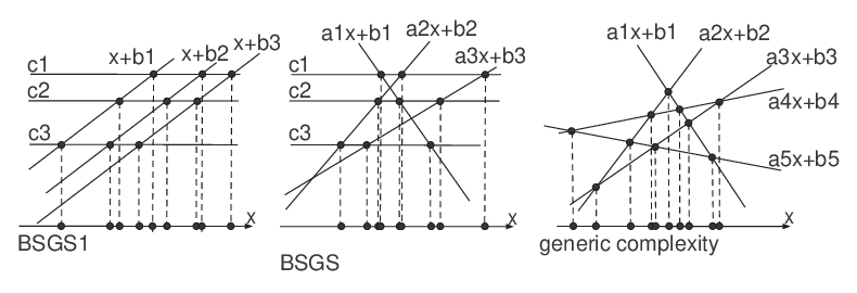
The problem of computing $\mathcal{C}_{\alpha}^{\textrm{{bsgs1}}}(S)$ is superficially similar to a number of problems in additive number theory concerned with studying properties of $X-Y$. However, our goal is fundamentally different since we require that $X-Y$ cover a large fraction of $S$ rather than be its exact equal. To the best of our knowledge, the only paper in the literature directly applicable to bounding $\mathcal{C}_{1}^{\textrm{{bsgs1}}}(S)$ is a 1977 paper by Erdös and Newman [EN77]. They proved analogues of our Theorems 3 and 6 and bounded the BSGS-1 complexity (in our notation) of the set of small squares $\{x^{2}\mid x<\sqrt{p}\}$ to be $\Omega(p^{1/3-c/\log\log p})$. They leave open the problem of constructing sets with a strictly linear BSGS-1 complexity (without the $1/\log p$ factor).

The BSGS and BSGS-1 complexities provide useful upper bounds for the generic complexity.

Consider, for example, the baby-step giant-step attacks on exponents with low Hamming weight [Hei93, Sti02]. Define $S_{\lambda}=\{x\in\mathbb{Z}_{p}\mid\nu(x)=\lambda|x|\}$, where $\nu(x)$ is the number of ones in the binary representation of $x$. Stinson [Sti02] estimates the complexity of the randomized algorithm due to Coppersmith to yield

For instance, if $\lambda=1/4$, the bound becomes $\mathcal{C}_{1/2}^{\textrm{{bsgs1}}}(S_{0.25})=\tilde{O}(p^{0.406})$.

Following Propositions 2, 3, and Theorem 3 the BSGS-1 $\alpha$-complexity of a set of cardinality less than $\sqrt{p}$ lies between $\sqrt{\alpha|S|/2}$ and $2\sqrt{\alpha p}$, where the lower bound is trivial and the upper bound is approximated up to a logarithmic factor by almost any subset of size $\sqrt{p}$. In this section we construct a set with succinct representation and a non-trivial BSGS-1 complexity. We start by stating without proof an important combinatorial lemma known as the Zarankiewicz problem [Zar51]:

Notice that the asymptotic of the bound on $Z(n,s,t)$ depends on the smallest of the two dimensions of the prohibited all-one submatrix. It is known that the bound is tight (up to a constant factor) for $t=2,3$.

Our second combinatorial tool follows from a more general upper bound due to A. Naor and Verstraëte on the number of edges in a bipartite graph without cycles of length $2k$ ($C_{2k}$-free graph):

When $k=2$ the two theorems overlap. Indeed, a 0-1 matrix is also a bipartite graph, where the rows and columns form the vertex set and the non-zero elements indicate adjacency of corresponding vertices. In this case an all-one $2\times 2$ submatrix represents a cycle of length 4 in the graph. Our theorems fully reflect this relationship: Theorem 6 can be proved using either the Zarankiewicz or the Naor-Verstraëte bound; its generalization Theorem 7 makes use of $C_{2k}$-free graphs, while Theorems 8 and 9 apply the Zarankiewicz bound.

We claim that $M$ does not contain an all-one $2\times 2$ submatrix. Assume the opposite: The submatrix given by elements $x_{1},x_{2}$ and $y_{1},y_{2}$ has four ones. It follows that all four $s_{11}=x_{1}-y_{1}$, $s_{12}=x_{1}-y_{2}$, $s_{21}=x_{2}-y_{1}$, $s_{22}=x_{2}-y_{2}\in S$. Then $s_{11}+s_{22}=s_{12}+s_{21}$, which contradicts the assumption that all pairwise sums of elements of $S$ are distinct. Applying the Zarankiewicz bound for the case $s=t=2$, we prove that

which implies that $n=\mathcal{C}_{\alpha}^{\textrm{{bsgs1}}}(S)>(\alpha|S|/\sqrt{2})^{2/3}$. $\!\square$

The sets where sums of pairs of different elements are distinct are known in combinatorics as weak Sidon sets. They are closely related to (strong) Sidon sets, also called $B_{2}$ sequences, where all pairwise sums (of not necessarily different elements) are distinct (for a comprehensive survey see [O’B04] that includes more than 120 bibliographic entries). Explicit constructions of Sidon subsets of $\{1,\dots,n\}$ due to Singer and Ruzsa have cardinality at least $\sqrt{n}-n^{.263}$ [Sin38, BC63, Ruz93, BHP01].

We additionally require that the sums be different modulo $p$. The size of such sets is bounded from above by $p^{1/2}+1$ [HHÖ04, Theorem 3]. The easiest shortcut to constructing weak modular Sidon sets is to take a strong Sidon subset of $\{0\dots\lfloor p/2\rfloor\}$ (see also [O’B02, Ch. 3] and [GS80]). Denser Sidon sets may be constructed for primes of the form $p=q^{2}+q+1$, where $q$ is also prime [Sin38]. Existence of infinitely many such primes is implied by Schinzel’s Hypothesis H and their density follows from the even stronger Bateman-Horn conjecture [Guy04, A]. Interestingly, modular Sidon sets are useful not only in constructing sets with high complexity, via Theorem 6, but also for solving the discrete logarithm problem in $\mathbb{Z}_{p}$ [CLS03].

Theorem 6 can be generalized to make use of Sidon sets of higher order. First, we prove that if all $k$-wise sums of elements of $S$ are distinct (counting permutations of the same $k$-tuple only once), then there is a bound on the BSGS-1 complexity. Second, we provide a result that there exist such sets of size $\mathrm{\Theta}(p^{1/k})$.

We claim that there are no $2k$-cycles (without repetitive edges) in the bipartite graph $G$. Assume the opposite: There is a cycle $(x_{1}$,$y_{1}$,…, $x_{k}$,$y_{k}$,$x_{1}$,$y_{1})$. Consider two sums: $(x_{1}-y_{1})+(x_{2}-y_{2})+\dots+(x_{k}-y_{k})$ and $(x_{2}-y_{1})+(x_{3}-y_{2})+\dots+(x_{k}-y_{k-1})+(x_{1}-y_{k})$. Not only are the two sums equal, they also consist of $k$ elements of $S$ each, and these elements are all distinct (as every element of $S$ appears as an edge of $G$ at most once). A contradiction is found.

The number of edges in an $(n,n)$-bipartite graph without $2k$-cycles is less than $2kn^{1+1/k}$ (Theorem 5). Therefore $\alpha|S|<2kn^{1+1/k}$, and $n=\mathcal{C}_{\alpha}^{\textrm{{bsgs1}}}(S)>(\alpha|S|/(2k))^{k/(k+1)}$. $\!\square$

Bose and Chowla give a construction for subsets of $\{1,\dots,q^{k}\}$ of prime size $q$ whose $k$-wise sums are distinct (in integers, not modulo $p$) [BC63]. By choosing the largest prime $q$ less than $p^{1/k}$ (which, for large $p$ is more than $p^{1/k}-p^{0.525/k}$ [BHP01]) an interval of length $q^{k}/k$ with a $1/k$ proportion of the set’s elements, we guarantee that all $k$-sums are distinct in $\mathbb{Z}_{p}$ as well. Unfortunately, [BC63] does not provide an efficient sampling algorithm.

Along the lines of Theorem 6 we prove that other verifiable criteria imply non-trivial bounds on the BSGS and generic complexity.

Constructing a large subset of $\mathbb{Z}_{p}$ with short description satisfying the condition of the previous theorem is a difficult problem. Fortunately, the probability that a random 6-tuple of $\mathbb{Z}_{p}$ elements fails to satisfy (1) is $2/p$ [Sch80]. This observation motivates the following definition:

Properties of $\mathcal{S}(N,k)$ are established in the following proposition:

2. Let $I_{ij}$ be the indicator variable, which is equal to 1 when $x_{i}=x_{j}$ and 0 otherwise. The cardinality of $S=\{x_{1},\dots,x_{N}\}$ is at least $N-\sum_{i<j}I_{ij}$. Since $x_{i}$ and $x_{j}$ are independent for all $i\neq j$, $E[I_{ij}]=1/p$. By linearity of expectation, the expected value $E[\sum_{i<j}I_{ij}]<N^{2}/p$. By Markov’s inequality $\Pr[|S|\neq N]=\Pr[\sum_{i<j}I_{ij}\geq 1]<N^{2}/p$.

3. Let $I_{i_{1},\dots,i_{k}}$ for all distinct $1\leq i_{1},\dots,i_{k}\leq N$ be the indicator variable that is 1 if and only if $h(x_{i_{1}}$,…,$x_{i_{k}})=0$. By independence of the variables and [Sch80] $E[I_{i_{1},\dots,i_{k}}]\leq 2/p$, which by linearity of expectation and Markov’s inequality implies that $\Pr_{S}[\exists\textrm{ distinct }x_{1},\dots,x_{k}\in S\textrm{ with }h(x_{1},\dots,x_{k})=0]\leq\Pr_{S}[\sum_{i_{1},\dots,i_{k}}I_{i_{1},\dots,i_{k}}\geq 1]<N^{k}d/p.$ $\!\square$

It follows that a randomly chosen set from the family $\mathcal{S}(p^{1/6-\varepsilon},6)$ has size $p^{1/6-\varepsilon}$ with probability at least $1-p^{-2/3}$ and satisfies the condition of Theorem 8 with probability at least $1-2p^{-6\varepsilon}$.

To apply a similar argument to the all-powerful generic complexity, we may show that for small constants $m_{1}$ and $m_{2}$, the projections on the $x$ axis of the intersection points of an irregular $m_{1}$ by $m_{2}$ grid (in which lines need not be parallel) satisfy a certain relationship. Next, a set $S$, where any $m_{1}m_{2}$-tuple avoids this relationship, is to be constructed.

Let us see first why this argument works for some values of $m_{1}$ and $m_{2}$, and then improve the parameters. Let $m_{1}=4$ and $m_{2}=5$. There are $9$ lines that can be described using 18 parameters. On the other hand, there are 20 points that form the intersection set of these lines. Each of the 20 intersection points imposes a linear equation on the parameters, and hence the system is overdetermined (even if we exclude linearly dependent equations). In particular, this implies that the probability that a random 20-tuple of elements of $\mathbb{Z}_{p}$ is coverable by a $4\times 5$ grid is negligible. We refine this argument in the following proposition.

If none of the lines is vertical, we can write down equations for all of them in the Cartesian coordinates. Let $l_{x,y,z}=\{a_{x,y,z}x+b_{x,y,z}\}$ and $l_{i}=\{c_{i}x+d_{i}\}$ for $1\leq i\leq 4$. Each intersection point imposes an equation on the parameters of the two lines incident with it, a total of 12 equations in 14 unknowns. However, the system always has a trivial solution, when all lines are equal. Rewrite the system using new variables: $\tilde{a}_{y}=a_{y}-a_{x}$, $\tilde{b}_{y}=b_{y}-b_{x}$, $\tilde{a}_{z}=a_{z}-a_{x}$, $\tilde{b}_{z}=b_{z}-b_{x}$, $\tilde{c}_{1}=c_{1}-a_{x}$, $\tilde{d}_{1}=d_{1}-b_{x}$, etc. The result is a homogenous system of 12 linear equations in 12 new variables. It has a non-zero solution if and only if its matrix is singular (only non-zero elements are shown):

References

- [BC63] Raj C. Bose and Sarvadaman Chowla. Theorems in the additive theory of numbers. Comment. Math. Helv., 37:141–147, 1962–1963.
- [BHP01] R. C. Baker, G. Harman, and J. Pintz. The difference between consecutive primes. II. Proc. London Math. Soc. (3), 83(3):532–562, 2001.
- [Bol98] Béla Bollobás. Modern graph theory, volume 184 of Graduate texts in mathematics. Springer, 1998.
- [CLP05] Jean-Sébastien Coron, David Lefranc, and Guillaume Poupard. A new baby-step giant-step algorithm and some applications to cryptanalysis. In Josyula R. Rao and Berk Sunar, editors, CHES 2005, volume 3659 of Lecture Notes in Computer Science, pages 47–60. Springer, 2005.
- [CLS03] M. Chateauneuf, Alan Ling, and Douglas R. Stinson. Slope packings and coverings, and generic algorithms for the discrete logarithm problem. J. Comb. Designs, 11(1):36–50, 2003.
- [CW77] Larry Carter and Mark N. Wegman. Universal classes of hash functions. In STOC 1977, pages 106–112, 1977.
- [EN77] Paul Erdös and Donald J. Newman. Bases for sets of integers. J. Number Theory, 9(4):420–425, 1977.
- [GS80] Ronald L. Graham and Neal J.A. Sloane. On additive bases and harmonious graphs. SIAM J. Algebraic and Discrete Methods, 1:382–404, 1980.
- [Guy04] Richard K. Guy. Unsolved Problems in Number Theory. Springer-Verlag, third edition, 2004.
- [Hei93] Rafi Heiman. A note on discrete logorithms with special structure. In Rainer A. Rueppel, editor, Advances in Cryptology—EUROCRYPT ’92, volume 658 of Lecture Notes in Computer Science, pages 454–457. Springer, 1993.
- [HHÖ04] Harri Haanpää, Antti Huima, and Patric R. J. Östergård. Sets in with distinct sums of pairs. Discrete Applied Mathematics, 138(1–2):99–106, 2004.
- [HS03] Jeffrey Hoffstein and Joseph H. Silverman. Random small Hamming weight products with applications to cryptography. Discrete Applied Mathematics, 130(1):37–49, 2003.
- [Knu97] Donald E. Knuth. Seminumerical Algorithms, volume 2 of The Art of Computer Programming. Addison-Wesley, third edition, 1997.
- [Nec94] Vassiliy I. Nechaev. Complexity of a determinate algorithm for the discrete logarithm. Math. Notes, 55(2):165–172, 1994.
- [NV05] Assaf Naor and Jacques Verstraëte. A note on bipartite graphs without -cycles. Probability, Combinatorics and Computing, 14(5–6):845–849, 2005.
- [O’B02] Kevin O’Bryant. Sidon Sets and Beatty Sequences. PhD thesis, U. of Illinois in Urbana-Champaign, 2002.
- [O’B04] Kevin O’Bryant. A complete annotated bibliography of work related to Sidon sequences. Electr. J. Combinatorics, DS11, July 2004.
- [Odl00] Andrew M. Odlyzko. Discrete logarithms: The past and the future. Des. Codes Cryptography, 19(2/3):129–145, 2000.
- [Pol78] John M. Pollard. Monte Carlo methods for index computation (mod ). Mathematics of Computation, 32:918–924, 1978.
- [Pol00] John M. Pollard. Kangaroos, monopoly and discrete logarithms. J. Cryptology, 13(4):437–447, 2000.
- [Ruz93] Imre Z. Ruzsa. Solving a linear equation in a set of integers. Part I. Acta Arith., 65:259–282, 1993.
- [Sch80] Jacob T. Schwartz. Fast probabilistic algorithms for verification of polynomial identities. J. ACM, 27(4):701–717, 1980.
- [Sch01] Claus-Peter Schnorr. Small generic hardcore subsets for the discrete logarithm. Inf. Process. Lett., 79(2):93–98, 2001.
- [Sha71] Daniel Shanks. Class number, a theory of factorization, and genera. In Donald J. Lewis, editor, 1969 Number Theory Institute, volume 20 of Proceedings of Symposia in Pure Mathematics, pages 415–440, Providence, Rhode Island, 1971. American Mathematical Society.
- [Sho97] Victor Shoup. Lower bounds for discrete logarithms and related problems. In Walter Fumy, editor, Advances in Cryptology—EUROCRYPT ’97, volume 1233 of Lecture Notes in Computer Science, pages 256–266. Springer, 1997.
- [Sin38] James Singer. A theorem in finite projective geometry and some applications to number theory. Trans. Amer. Math. Soc., 43:377–385, 1938.
- [SJ04] Yaron Sella and Markus Jakobsson. Constrained and constant ratio hash functions. Manuscript, 2004.
- [Sti02] Douglas R. Stinson. Some baby-step giant-step algorithms for the low Hamming weight discrete logarithm problem. Math. Comput., 71(237):379–391, 2002.
- [SWD96] Oliver Schirokauer, Damian Weber, and Thomas F. Denny. Discrete logarithms: The effectiveness of the index calculus method. In H. Cohen, editor, ANTS-II, volume 1122 of Lecture Notes in Computer Science, pages 337–361. Springer, 1996.
- [Tes01] Edlyn Teske. Square-root algorithms for the discrete logarithm problem (a survey). In Public-Key Cryptography and Computational Number Theory, pages 283–301, 2001.
- [vOW99] Paul C. van Oorschot and Michael J. Wiener. Parallel collision search with cryptanalytic applications. J. Cryptology, 12(1):1–28, 1999.
- [Yac98] Yacov Yacobi. Fast exponentiation using data compression. SIAM J. Comput., 28(2):700–703, 1998.
- [Zar51] Kazimierz Zarankiewicz. Problem P 101. Colloq. Math., 2:301, 1951.
Appendix A Bipartite Menelaus’ Theorem
Let us first recap the classic Menelaus theorem.
Theorem 10 (Classic Menelaus)
Consider four directed lines intersecting at six points (see Fig. 4a). Then