An Algorithmic Approach to Non-self-financing Hedging in a Discrete-Time Incomplete Market
Abstract
We present an algorithm producing a dynamic non-self-financing hedging strategy in an incomplete market corresponding to investor-relevant risk criterion. The optimization is a two stage process that first determines admissible model parameters that correspond to the market price of the option being hedged. The second stage applies various merit functions to bootstrapped samples of model residuals to choose an optimal set of model parameters from the admissible set. Results are presented for options traded on the New York Stock Exchange.
1 Introduction
Pricing and hedging of financial assets in incomplete markets is an active research area in mathematical finance. One of the possible ways to produce a model of an incomplete market in discrete time setting is to assume that stock price relative changes (jumps) can take more that two values as opposed to the classical binomial model of Cox-Ross-Rubinstein. In [1], [2], and [3] an incomplete market in which stock price jumps follow a multinomial distribution is studied. In [1] the no-arbitrage option price interval is studied, [2] and [3] discuss risk minimization aspects in option pricing and hedging.
The multinomial model has been further extended to the case where stock price jumps are distributed over a bounded interval and options under consideration have convex pay-off functions. In [4], the upper and lower bounds for no-arbitrage prices of a European contingent claim with convex pay-off are obtained. The series of works by A. Nagaev et al. (see [5], [6], [7], and [8]) are devoted to asymptotic behavior of the residual value of a minimum cost super-hedge. The residual value occurs as a result of non-self-financing dynamic hedging strategy of an option seller introduced and discussed in [5].
A significant proportion of research on option pricing and hedging in incomplete markets constructs self-financing trading strategies that satisfy both a primary no-arbitrage condition and secondary conditions on portfolio risk and return. A comprehensive survey of modern methodologies can be found in [9]. A number of articles that deal with frictions in markets, shortfall risks and quadratic hedging (all producing incomplete markets) can be found in the recent compendium [10].
Less prevalent is the study of non-self-financing trading strategies in similar economic environments. The encyclopedic reference [11] and the more modest [12] both illuminate option pricing with consumption, the model which is similar to the work presented here. Our work is an initial investigation in the algorithmic study of non-self-financing strategies discussed in [5] and [8]. We explore the short term behavior of the residual value of a minimum cost super-hedge, whose long term behavior was studied by Nagaev et al.
Assuming independent and identically distributed jumps in the underlying stock process, we use historical data and a bootstrap simulation process to develop an algorithm producing a dynamic non-self financing hedging strategy. The resulting hedging strategy constructs a residual sequence with improved investor risk criteria as compared to other possible hedging strategies. No additional assumptions are placed on the underlying stock price jump process other than having bounded support. An algorithmic approach similar to our use of bootstrap simulation, but having a different theoretical foundation and goals can be found in [13].
The remainder of the paper is organized as follows. We develop the discrete time financial model in section 2. The notion of the residual value of a minimum cost super-hedge is developed in sections 3 through 5. The algorithm is described in section 6. Algorithm implementation and illustrative results are presented in 7. We conclude with some remarks in section 8 and directions for further study in section 9.
2 Discrete Time Financial Model
Following the theoretical development in [5], our discrete time financial model consists of two fundamental assets and a derivative security.
- 1.
A risk-free bond with fixed interest rate , evolving from an initial value at time to at time as
- 2.
A risky stock evolving from an initial value at time to at time as
where are assumed to be independent and identically distributed random variables with probability distribution having support equal to a bounded interval . No further assumptions are made on the distribution function for the . However, this assumption is sufficient to render our financial market incomplete.
- 3.
A derivative security with convex payoff function . For our numerical investigations, we use a European call option on the stock. We take the position of an option seller who wishes to hedge the potential liability of the sold derivative being exercised.
Our goal is to develop and evaluate an algorithm that will determine a dynamic, non-self-financing hedging strategy consisting of a portfolio of our stock and bond assets in our incomplete market. The portfolio will approximately hedge the derivative security and will satisfy additional criteria, based on the deviation of the portfolio value from the required hedging value, that are meaningful to the investor.
3 Super-hedging Portfolio
Based on a convexity argument, [5] showed that when the parameters and are known, there is a minimum cost super-hedge whose value at every time instant is greater than or equal to the value of the derivative security. This super-hedge is a portfolio of stocks and bonds at time described by
| (1) |
| (2) |
where
| (3) |
| (4) |
is the number of periods to expiration, is the binomial coefficient, and is a convex pay-off function. At each time instant , the dynamic super-hedge portfolio constructed in the prior period is liquidated and the proceeds are used to construct a new portfolio for the current period. The liquidation value of the prior period portfolio is given by
| (5) | |||||
The funds required to construct the new period portfolio, or set-up cost, is given by
| (6) |
(see section 4 for more detail). The liquidation value (5) will exceed the set-up cost (6) producing a residual amount
| (7) |
In this case where and are known, and consequently it follows from the convexity of the pay-off function that the residual is non-negative:
| (8) |
In this fashion, each stock price process path maps to a corresponding sequence of non-negative residuals , which are withdrawn after each portfolio liquidation prior to the construction of the next time period super-hedge. The accumulated value of the withdrawn residuals at maturity is given by
| (9) |
For the remainder of this paper we will assume a European call option pay-off function
| (10) |
where is the option strike price.
4 Model Properties
Ruschendorf [4] and Nagaev [5] document a number of properties of our financial market model which will illuminate our algorithmic design approach. In particular, the incompleteness of the market model is manifested in an open interval of no-arbitrage option prices. The end points of the interval are shown to be
where is the option strike price and is defined in (3).
At every time instant , the open interval is the set of no-arbitrage option prices. For the option seller, the upper bound is the demarcation between risk sharing with the option buyer (if the option sale price is below ) and the potential for arbitrage profit (if the option sale price is at or above ).
Let us now replace the parameters with a pair of numbers such that
| (11) |
and let us construct the portfolio with the time set-up cost
| (12) |
where is defined in (3). It is straightforward to show that for any choice of and satisfying (11), the resulting portfolio set-up cost (12) falls within the no-arbitrage option price interval
We will refer to the value as a rational price of the option.
5 Choice of Pair
As a practical matter, we do not know the actual values of and . Suppose we choose a pair that is within the and values:
and suppose that for any given stock price process we define the hedging portfolio strategy
| (13) |
where and are defined in (1) and (2) respectively, with the boundary parameters replaced with the values . The above portfolio strategy will produce a residual sequence
| (14) |
where is defined in (7), with replaced by . It is straightforward to show that
- •
if
- •
if or
- •
if or
In order to maintain the dynamic portfolio strategy defined by (13), at each time step the investor will withdraw the residual (14) from the liquidated proceeds when and add the amount when . The risk-free growth of the local residuals produces an accumulated residual defined by
| (15) |
We would like to stress here that the hedging portfolio strategy constructed above is in general non-self-financing. An investor who utilizes our dynamic hedging strategy will want to choose values for and that determine a residual sequence with desirable statistical characteristics. It is the choice of the model parameter values and based on the statistical characteristics of the residual sequence that constitutes our algorithm design.
6 Risk Minimization on Contours
We propose a two-stage algorithm for choosing a pair. The first stage reduces the set of pairs under consideration by imposing a market calibration constraint. The second stage chooses from this reduced set a pair that optimizes one of a number of investor-relevant statistical properties of the residual sequence.
6.1 Market Calibrated Price Contour
The first stage of our proposed risk minimization procedure is the selection of a set of pairs consistent with the quoted market option price.
Each pair uniquely determines a portfolio strategy that is dependent upon the realized values of the stock and bond processes. At the initial time , the portfolio strategy determined by a pair specifies an initial portfolio consisting of bonds and stocks where and are defined in (2) and (1) with and At time the set-up cost of the so constructed portfolio is
| (16) |
where is given by (4) (with replaced by ) and is the stock price at To calibrate the choice of pairs to the market price of the option, we need to set equal to the option time market price
While the choice of uniquely determines a portfolio set-up cost, specifying a portfolio set-up cost determines a contour of pairs since there are a multiplicity of portfolios with identical set-up costs. This contour consists of the set
Computationally, we utilize contour construction software to compute a finite number of pairs satisfying (17). It is this set of pairs that is used by the second stage of our algorithm.

6.2 Investor-relevant Choice Criteria
The second stage of the two-stage algorithm selects a unique pair on the market calibrated contour defined in (17) that optimizes one of several investor risk criteria. Each pair on the market-calibrated contour determines a dynamic hedging portfolio strategy. For a given stock price process , the -determined portfolios produce a sequence of residuals each representing a residual profit/loss for an investor (see section 5 for details). This sequence is an economic measure of the consequence of choosing model parameters and the associated dynamic hedging portfolio.
There are several criteria that convert this sequence into a scalar measure of investor risk, each reflecting some aspect of the option seller attitude towards risk. We thus have the following situation. Fix a pair at time . Each potential stock price time series determines a sequence of residuals . A particular choice of a risk criterion reduces the sequence to a single scalar value of risk. To judge the acceptability of the pair under the chosen risk measure, we simulate a number of stock price time series and collect the corresponding sample of scalar risk values. An appropriate sample statistic (mean value or probability of a desirable event) is then computed from the sample as the utility value of the pair. The behavior of the sample statistic as the pair is varied over the market-calibrated contour determines the optimal choice of .
There are four criteria that we consider for choosing a unique pair.
- •
Maximize the likelihood of a positive accumulated residual:
(19) - •
Minimize expected shortfall:
(20) - •
Minimize the expected accumulated squared residuals:
(21) - •
Maximize the expected accumulated profit
(22)
The first criterion (19) interprets a positive residual as a profit, and chooses a pair that has the highest probability of a net profit. In the absence of arbitrage a large accumulated profit is not attainable with high probability. There is the possibility, however, of an investor achieving a small positive profit. The optimization problem presented here produces a market calibrated hedging strategy that maximizes the likelihood of a positive accumulated profit.
The second criterion (20) reflects an investor’s desire to minimize the amount of single period additional funding needed to rebalance the portfolio over the life of the option. A negative residual represents the cash shortfall of the portfolio value at time The largest negative is the largest shortfall value. Optimizing this criterion produces a hedging portfolio with minimal expected single period additional funding.
In (21) the residual represents an economic measure of model error. Concern for minimizing model risk would motivate weighting equally positive and negative residuals. Indifference to the sign of can be achieved by using squared residuals in the risk criterion.
Our final criterion (22) maximizes the expected accumulated residual, which reflects total net profit from using the dynamic portfolio based on the chosen . It was shown in [5] that the expected accumulated profit is asymptotically constant on contours of constant rational price. We thus anticipate minimal differences in the expected accumulated profit at each pair on our constant rational price contours when is large. For small empirical results show it is possible to have a market contour with non-constant expected accumulated profit.
In summary, our model provides a measure of the economic impact of market incompleteness by the construction of the residuals . The criteria presented here can be optimized to determine hedging strategies that mitigate investor risk.
7 Algorithm Implementation and Numerical Results
In this section, we present an implementation of our two-stage algorithm for producing an optimal hedging strategy as measured by the risk criteria presented in section 6.2. Following this is a presentation of illustrative results from applying the algorithm to real market data.
7.1 Two-stage Algorithm
The choice of an optimal pair proceeds in two stages.
- •
Reduction by market calibration of the population of pairs to a contour given by (17) corresponding to the quoted market option price.
- •
Imposition of a ranking criterion, based on a bootstrap estimated statistic of the residual sequence.
The numerical procedures to be described are implemented in the R computer language ([14]). The flow of computation proceeds as follows.
- 1.
The contour creation function in R is applied to the normalized value surface given in (18). Contours defined by (17) with are identified as depicted in Figure 1. The contour matching the market option price is chosen. The software typically identifies between 80 and 100 pairs on the market calibrated contour.
- 2.
Historical daily stock price data is used to create a sequence of daily stock price jumps. The jumps are separated into groups by day count of successive price data: next day jumps (e.g. Monday to Tuesday price jump) and weekend jumps (i.e. Friday to Monday price jump) constitute the majority of jumps. There are a few single day mid-week holiday jumps and long weekend jumps. A typical stock price process and jump process are depicted in Figure 2.

Stock Price Time Series 
Jump Distributions Figure 2: Stock Price Process and Price Jump Process - 3.
Each of the next day and weekend groups are sampled with replacement to form bootstrap jump sequences (four next-day jumps followed by one weekend jump, repeated for however many weeks of bootstrap data are needed). Each jump sequence uniquely determines a stock price sequence. A set of bootstrap jump and price processes are depicted in Figure 3.
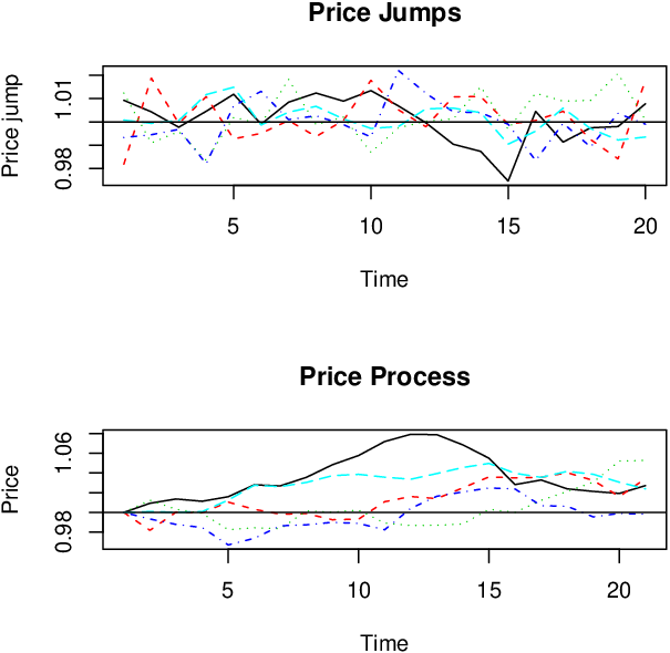
Figure 3: Bootstrap Stock Price Processes 
Figure 4: Local residual () distribution 
Figure 5: Aggregated Residual () Distribution - 4.
- 5.
Each criteria is applied to the bootstrap sample of residual sequences and the appropriate statistic (expected value or probability) is estimated.
- 6.
The pair with the best criterion value is chosen. This results in four optimal pairs, one for each of the four criteria described previously.
7.2 Illustrative Results
In this section we present results representative of the insight obtained from applying the risk evaluation tools developed in previous sections. Results are shown for several call options traded on the New York Stock Exchange expiring on October 15, 2004. The selected options are as follows
- •
Walmart corporation option WMT+JJ, strike price $50
- •
Exxon Mobil corporation option XOM+JV, strike price $42.50
- •
Intel corporation option INQ+JE strike, price $25.
Data collected included historical stock price data, option strike price and market option price. Over 500 daily stock prices were recorded and used in constructing bootstrap samples of the stock price jump process. The market option price data for a period of 40 days prior to expiration was collected and used in selecting market calibrated contours (as described in section 7.1) with varying time to expiration. The market option price days prior to expiration was used in identifying the appropriate contour for each of the reported values of
Selecting a market calibrated contour produces a set of approximately 80 pairs each corresponding to a potential hedging portfolio. The risk criteria (19) through (22) are evaluated for each hedging portfolio and the optimal is chosen. Table 1 presents results for the Exxon-Mobil option with days to expiration. The algorithm produces a hedging portfolio where the probability of a positive profit is 1. This is consistent with the theoretical results presented in section 5. When the sequence of relative stock price jumps fall within the interval we are guaranteed the local residual profits will be positive. The optimal expected shortfall and expected squared deviation are both essentially zero. For this particular data the objective values along the contour did not vary dramatically. The advantage of utilizing the algorithm is seen in the expected shortfall computation where the optimal expected shortfall is approximately 3 times as small as other possible shortfall values.
| Risk criterion | Optimal (u,d) | Objective value |
|---|---|---|
| (1.0112,0.9792) | 1.0 | |
| (1.0146,0.9834) | -0.0042 | |
| (1.0130,0.9822) | 0.0053 | |
| (1.0100,0.9961) | 0.2066 |
Results for the Walmart option are presented in tables 2 through 4. Examining the results we see that for and days to expiration, the optimal pair produces with probability a small positive aggregated profit. It is interesting to note that over all pairs on the contour, the probability of a positive aggregated profit ranged from approximately 0.6 to 1.0 when and and from approximately 0.3 to 0.99 when In other words, an investor can increase the probability of achieving a small positive profit from 0.3 to 0.99 by following the hedging strategy produced by the algorithm.
Similar results were seen in comparing the values of the other risk criteria for the optimal hedging portfolio as compared to other hedging portfolios associated with pairs on the contour. In particular, considering the Walmart data with days to expiration, the values for the expected shortfall ranged from -0.0548 (see the second column of 2) to approximately -0.4. The shortfall is more than 7 times as large as the optimal for some hedging portfolios. The values of the expected squared deviation ranged from the minimum of 0.0225 to a maximum of approximately 0.18 and the expected aggregated profit ranged from approximately 0 to 0.3. These results illustrate the value of following the hedging strategy suggested by the algorithm.
| Risk criterion | Optimal (u,d) | Objective value |
|---|---|---|
| (1.0156,0.9897) | 1.0 | |
| (1.0140,0.9889) | -0.0548 | |
| (1.0134,0.9881) | 0.0225 | |
| (1.0076,0.9804) | 0.3097 |
| Risk criterion | Optimal (u,d) | Objective value |
|---|---|---|
| (1.0171,0.9901) | 1.0 | |
| (1.0136,0.9878) | -0.0355 | |
| (1.0136,0.9878) | 0.0220 | |
| (1.0052,0.9718) | 0.2372 |
| Risk criterion | Optimal (u,d) | Objective value |
|---|---|---|
| (1.0238,0.9882) | 0.99 | |
| (1.0178,0.9857) | -0.0018 | |
| (1.0116,0.9820) | 0.0054 | |
| (1.0068,0.9747) | 0.0215 |
Comparing tables 2 through 4 we see that the optimal objective function value for most of the risk criteria does not change much as the length of time to expiration changes with the exception of the expected aggregated profit. The value for is more than 10 times larger than the value for . The difference could be explained by the fact that given more time to expiration, there are more opportunities to withdraw a small positive profit (at each ). If we consider the results produced for the Intel option for and presented in tables 5 through 7, we do not see the same change in the value of the expected aggregated profit. In this case, however, the probability of achieving a positive profit is more variable with the length of time to expiration increasing from 0.8 to 0.93 as decreases from to Clearly, the behavior of the optimal objective values vary with each chosen option.
| Risk criterion | Optimal (u,d) | Objective value |
|---|---|---|
| (1.0140,0.9640) | 0.8 | |
| (1.0130,0.9616) | -0.0378 | |
| (1.0160,0.9696) | 0.0104 | |
| (1.0127,0.9608) | 0.0429 |
| Risk criterion | Optimal (u,d) | Objective value |
|---|---|---|
| (1.0193,0.9624) | 0.83 | |
| (1.0182,0.9600) | -0.0098 | |
| (1.0229,0.9703) | 0.0045 | |
| (1.0197,0.9632) | 0.0253 |
| Risk criterion | Optimal (u,d) | Objective value |
|---|---|---|
| (1.0339,0.9600) | 0.93 | |
| (1.0130,0.9616) | -0.0034 | |
| (1.0160,0.9696) | 0.0062 | |
| (1.0127,0.9608) | 0.0475 |
8 Conclusions
We have developed an algorithm that produces a non-self-financing hedging strategy in an incomplete market corresponding to one of several investor risk criteria. The algorithm provides the opportunity to evaluate the economic consequences of choosing a particular hedging strategy in an incomplete market. The two-stage algorithm optimizes one of a number of investor-relevant statistical properties of a local residual profit or shortfall.
The algorithm was tested on several options traded on the New York stock exchange. The results illustrate that following the portfolio strategy produced by the algorithm is beneficial to an investor, improving the value of the investor risk criterion by as much as a factor of ten compared to the results associated with other, non-optimal hedging portfolio strategies.
9 Future Research
In this paper we investigate non-self financing hedging strategies for a short-term European call option (time to expiration, is at most 30 days). Our algorithm builds a short-term portfolio strategy that optimizes one of the investor-related criteria. Our research was inspired by theoretical investigations of A. Nagaev et al. (see [5], [6], [7], [8]) where the long-term behavior (large ) of the accumulated residual (15) has been studied.
In [5], [6], and [7], asymptotic properties of the so-called riskless profit of an investor ( defined in (9) with the boundary parameters and ) have been studied. The case of independent identically distributed (i.i.d.) stock price jumps is presented in [5]; in [6] the jumps are assumed to follow a discrete Markov chain; [7] studies the case of independent, but not identically distributed jumps. In all three cases, by means of suitable diffusion approximations, asymptotic formulas for the mean accumulated residuals in terms of the original model parameters have been obtained.
In [8], A. Nagaev considers the accumulated residual (15) for the case of non-boundary parameters and satisfying (11) (the so-called risky profit of an investor). In this case, under the i.i.d. assumptions on the stock price jumps, the asymptotic formula for the mean accumulated residual has been obtained and asymptotic connections (as time to expiration tends to infinity) between and the set-up cost have been established.
The present paper is an initial study of the short-term accumulated residuals. We assume here that the relative stock price jumps are i.i.d. random variables and build our bootstrap simulation procedure accordingly. In the future we will investigate the consequences of more realistic assumptions on stock price jumps using methods of time series analysis and/or advanced model fitting (e.g. Levy processes based probability models). We also plan to extend our investigations to other derivative securities with convex pay-off functions. An additional direction of future research is numerical testing of the asymptotic formulas obtained by A. Nagaev et al., more specifically, exploring the consequences of the finite number of time steps to expiration on asymptotic results.
10 Acknowledgements
We would like to dedicate this paper to our colleague, Alexander Nagaev. Alexander was an insightful mathematician, creative thinker and a true friend. He died unexpectedly in 2005 and we truly miss him.
This work is partially supported by Bentley College Enterprise Risk Management Research Grants.
References
- [1] G. Tessitore and J. Zabczyk, “Pricing options for multinomial models,” Bulletin of the Polish Academy of Sciences Mathematics, vol. 44, no. 3, pp. 363–380, 1996.
- [2] G. Wolczynska, “An explicit formula for option pricing in discrete incomplete markets,” International Journal of Theoretical and Applied Finance, vol. 1, no. 2, pp. 283–288, 1998.
- [3] O. Hammarlid, “On minimizing risk in incomplete markets,” International Journal of Theoretical and Applied Finance, vol. 1, no. 2, pp. 227–233, 1998.
- [4] L. Ruschendorf, “On upper and lower prices in discrete time models,” Proc. Steklov Math. Inst., vol. 237, pp. 134–139, 2002.
- [5] A. Nagaev and S. Nagaev, “Asymptotics of riskless profit under selling of discrete time call options,” Applicationnes Mathematicae, vol. 30, no. 2, pp. 173–191, 2003.
- [6] S. Nagaev, A.V. Nagaev and R. Kunst, “A diffusion approximation to the Markov chain model of the financial market and the expected riskless profit under selling of call and put options,” Preprint 164, Economics Series, Institute for Advanced Studies, Vienna, January 2005.
- [7] ——, “A diffusion approximation to the riskless profit under selling of discrete time call options: Non-identically distributed jumps,” Preprint 164, Economics Series, Institute for Advanced Studies, Vienna, January 2005.
- [8] A. Nagaev, “A diffusion approximation of the expected risky profit on an investor under selling of discrete time options (manuscript in Russian).”
- [9] J. Staum, “Incomplete markets,” preprint submitted to Elsevier Science available http://users.iems.northwestern.edu/ staum/IncompleteMarkets.pdf.
- [10] M. M. E. Jouini, J. Cvitanic, Ed., Option Pricing, Interest Rates and Risk Management. Cambridge University Press, 2001.
- [11] A. N. Shiryaev, Essentials of Stochastic Finance: Facts, Models, Theory. World Scientific, 1999.
- [12] A. Melnikov, S. Volkov, and M. Nechaev, Mathematics of Financial Obligations. American Mathematical Society, 2002.
- [13] S. Sergey and S. Uryasev, “Pricing derivative securities in incomplete markets,” in Proceedings of the 2004 Winter Simulation Conference, 2004.
- [14] R. D. C. Team, R: A Language and Environment for Statistical Computing, 2005. [Online]. Available: www.R-project.org