Five Lectures on Khovanov Homology
Abstract.
These five lectures provide an introduction to Khovanov homology covering the basic definitions, important properties, a number of variants and some applications. At the end of each lecture the reader is referred to the relevant literature for further reading.
About these lectures
These lectures were designed for the summer school Heegaard-Floer homology and Khovanov homology in Marseilles, 29th May - 2nd June, 2006.
The intended audience is graduate students with some minimal background in low-dimensional and algebraic topology. I hesitated to produce lecture notes at all, since much of the literature in the subject is very well written, but decided in the end that notes could serve some purpose.
In order to keep the narrative flowing I found it convenient to delay all attributions of credit until the end of each lecture. I have attempted to do this as accurately as possible and if I have failed to properly attribute a certain piece of work or omitted to mention someone in a particular context, my apologies to the injured party in advance.
At the present time the pace of development of the subject is very rapid and the reader is encouraged to consult math/GT for the latest developments.
Many thanks F. Costantino, M. Mackaay and P. Vaz for their comments on a draft version and to D. Matignon for organising a very stimulating summer school.
Paul Turner
School of Mathematical and Computer Sciences
Heriot-Watt University
Edinburgh EH14 4AS
Scotland
Chapter 1 Lecture One
In this lecture we begin with a very brief introduction to the subject, followed by some recollections about the Jones polynomial. We then define the main object of interest: the Khovanov complex of an oriented link diagram.
1.1. What is it all about?
Given an oriented link diagram, , Khovanov constructs in a purely combinatorial way a bi-graded chain complex associated to .
Given a chain complex we can apply homology to it and for this results in the Khovanov homology, , of the diagram .
The following properties are satisfied:
- (1)
If is related to another diagram by a sequence of Reidemeister moves then there is an isomorphism
- (2)
The graded Euler characteristic is the unnormalised Jones polynomial i.e.
You should think, by way of analogy, of the relationship of the ordinary Euler characteristic to homology. For a space (there are some restrictions on , say, a finite CW complex) we can assign a numerical invariant, the Euler characteristic . This can be calculated by a simple algorithm based on some combinatorial information about the space (eg the CW structure, a triangulation etc). On the other hand, homology assigns a graded vector space to and is related to the Euler characteristic by the formula:
In this way homology categorifies the Euler characteristic: a number gets replaced by a (graded) vector space whose (graded) dimension gives back the number you started with.
In the case of links we can assign quantum invariants such as the Jones polynomial. These can be calculated by a simple algorithm based on some combinatorial information about the link (e.g. a diagram). Khovanov homology is the analogue of homology and categorifies the Jones polynomial.
Homology has many advantages over the Euler characteristic. For example
- •
homology is a stronger invariant than the Euler characteristic,
- •
homology reveals richer information e.g. torsion,
- •
homology is a functor.
As we will see soon, Khovanov homology has similar advantages over the Jones polynomial.
1.2. Recollections about the Jones polynomial
Let be an oriented link and a diagram for with
crossings. Suppose that of these are negative crossings (like
this: ![[Uncaptioned image]](0606464v1/negative.png) ) and are positive (like this:
) and are positive (like this:
![[Uncaptioned image]](0606464v1/positive.png) ). The Kauffman bracket of the diagram , written is the Laurent polynomial in a variable (i.e. ) defined recursively by:
). The Kauffman bracket of the diagram , written is the Laurent polynomial in a variable (i.e. ) defined recursively by:
| (1.1) | |||||
| (1.2) |
(Beware: this is not the usual normalisation).
The Kauffman bracket is not a link invariant but by defining
one gets a genuine link invariant i.e. something invariant under all the Reidemeister moves. The Jones polynomial is given by
(The usual formula for the Jones polynomial involves a variable . Substitute to make the descriptions match). The polynomial is known as the unnormalised Jones polynomial.
Equation (1.1) reduces the number of crossings at the expense of twice as many terms on the right hand side. For a diagram with crossings we can apply this equation times to end up with pictures on the right hand side each of them consisting of a collection of circles in the plane which we then evaluate using Equation (1.2).
To do this in a systematic way let us agree that given a crossing
(looking like this: ![[Uncaptioned image]](0606464v1/crossing.png) ) we will call the two
pictures on the right of Equation (1.1) the 0-smoothing
(looking like this:
) we will call the two
pictures on the right of Equation (1.1) the 0-smoothing
(looking like this:
![[Uncaptioned image]](0606464v1/smoothing0.png) ) and the 1-smoothing (looking like this:
) and the 1-smoothing (looking like this:
![[Uncaptioned image]](0606464v1/smoothing1.png) ).
).
Thus, if we number the crossings of by then each of the pictures can be indexed by a word of zeroes and ones i.e. an element of . We will call a picture in which each crossing has been resolved (in one of the two ways above) a smoothing. Thus a diagram has smoothings indexed by . The set is the vertex set of a hyper-cube as shown in Figure 1.1, with an edge between words differing in exactly one place.

It is convenient to think of the smoothings as living on the vertices of this cube. For we will denote the associated smoothing (the collection of circles in the plane) by . Given we define
and
We can now use Equations (1.1) and (1.2) to write down a state-sum expression for .
Exercise 1.2.1.
Convince yourself that this above state-sum formula is correct.
Example 1.2.2.
Consider the Hopf link ![[Uncaptioned image]](0606464v1/hopflink.png) which has and . There are four pictures which we assemble on the vertices of a square as displayed in Figure 1.2 and we compute the unnormalised Jones polynomial to be
which has and . There are four pictures which we assemble on the vertices of a square as displayed in Figure 1.2 and we compute the unnormalised Jones polynomial to be

Exercise 1.2.3.
Write out the cube of smoothings for ![[Uncaptioned image]](0606464v1/trefoil.png) and use the state-sum formula to compute the unnormalised Jones polynomial.
and use the state-sum formula to compute the unnormalised Jones polynomial.
1.3. The definition of the Khovanov complex of a link diagram
For the time being we will work over , so “vector space” means “ vector space over ”. Khovanov’s idea is to assign a cochain complex to a link diagram . The homotopy type of this complex will turn out to be an invariant and its graded Euler characteristic the unnormalised Jones polynomial.
Before getting to the definition let’s recall a few things about finite dimensional graded vector spaces.
- (1)
The graded (or quantum) dimension, qdim, of a graded vector space is the polynomial in defined by
- (2)
The graded dimension satisfies
- (3)
For a graded vector space and an integer we can define a new graded vector space (a shifted version of ) by
Notice that .
Now we turn to the definition of the Khovanov complex, , of an oriented link diagram . An important role is played by the following two-dimensional graded vector space. Let (the -vector space with basis and ) and grade the two basis elements by and .
Exercise 1.3.1.
Show that .
Recall that we have smoothings of our diagram. To each now associate the graded vector space
and define
The internal grading comes from the fact that each is a graded vector space. Note that the vector spaces are trivial outside the range .
Recall that in the last section we arranged the smoothings of the diagram on a cube with vertices indexed by . The above definition means that we now replace the smoothing with the vector space so that the space is the direct sum of vector spaces in column of the cube as indicated in Figure 1.3.


An element of is said to have homological grading and -grading . If with homological grading and -grading then it is useful to remember that
where deg is the degree of as an element of .
What we need now is a differential turning into a complex. Recall that we have a smoothing (i.e. a collection of circles) associated to each vertex of the cube . Now to each edge of the cube we associate a cobordism (i.e. an (orientable) surface whose boundary is the union of the circles in the smoothings at either end).
Edges of the cube can be labelled by a string of zeroes and ones with a star () at the position that changes. For example the edge joining to is denoted . We can turn edges into arrows by the rule: gives the tail and gives the head. For an arrow note that the smoothings and are identical except for a small disc (the changing disc) around the crossing that changes from a 0- to a 1-smoothing (the one marked by a in ). For example the changing disc for the arrow in the cube (square!) of the Hopf link above is shown in Figure 1.5.

The cobordism associated to is defined to be the following surface: outside the changing disc take the product of with the unit interval and then plug the missing tube with the saddle ![[Uncaptioned image]](0606464v1/saddle.png) Thus each consists
of a bunch of cylinders and one pair-of-pants surface
(
Thus each consists
of a bunch of cylinders and one pair-of-pants surface
(![[Uncaptioned image]](0606464v1/pants1.png) or
or
![[Uncaptioned image]](0606464v1/pants2.png) ).
).
Cobordism convention: pictures of cobordisms go down the page.
Above we replaced the smoothing by the vector space and now we will replace the cobordism associated to the edge by a linear map . Since each circle in a smoothing has a copy of the vector space attached to it, to define we only require two linear maps: one that fuses and one that splits . Then we can define to be the identity on circles not entering the changing disc and either or on the circles appearing in the changing disc (depending on whether the pair-of-pants has two or one input boundary circles).
We define by
and by
In fact by defining a unit and counit and we have endowed with the structure of a commutative Frobenius algebra. Isomorphism classes of commutative Frobenius algebras are in bijective correspondence with isomorphisms classes of 1+1-dimensional topological quantum field theories so what we are really doing here is applying a TQFT (the one defined by ) to the cube of circles and cobordisms - more on this in Lecture 2.
We are finally ready to define . For set
where .
Proposition 1.3.3.
.
Proof.
(sketch) The idea of the proof is that without the signs each face of the cube commutes. To see this one can either look at a number of cases and use the definition of the maps and or (much better) begin to think geometrically: each of the two routes around a face gives the same cobordism (up to homeomorphism) and so applying the TQFT defined by gives the same linear map. Once all the non-signed faces commute then observe that the signs occur in odd numbers on every face, thus turning commutativity into anti-commutativity. ∎
Exercise 1.3.4.
Write out the above proof properly - you may wish to wait until after Lecture 2 where there is a more detailed discussion of Frobenius algebras and TQFTs.
Exercise 1.3.5.
Check that has bi-grading .
The graded Euler characteristic of this complex i.e.
is nothing other than the unnormalised Jones polynomial.
Exercise 1.3.6.
Convince yourself that the previous statement is true - this is simply a matter of unwinding the definitions and then comparing with the state-sum formula for the unnormalised Jones polynomial.
Later we will see that the homotopy type of is invariant under transformations by Reidemeister moves. For now, to end this lecture, let us perform a homology calculation.
Example 1.3.7.
Let us compute the homology of . The complex has only three non-trivial terms:
More explicitly we have:
and based on this one can compute as follows.
| Homological degree | -2 | -1 | 0 |
|---|---|---|---|
| Cycles | |||
| Boundaries | - | ||
| Homology | - | ||
| -degrees | -4, -6 | 0, -2 |
The homology can be summarised as a table where the homological degree is horizontal and the -degree vertical.
| -2 | -1 | 0 | |
|---|---|---|---|
| 0 | |||
| -1 | |||
| -2 | |||
| -3 | |||
| -4 | |||
| -5 | |||
| -6 |
Exercise 1.3.8.
Write out the cube for the trefoil explicitly (including the correct signs on the edges). Calculate the homology of the Khovanov complex. This involves a bit of work, but is a very good test to see if you have understood all the definitions.
1.4. Notes and further reading
The original paper by Khovanov in which he defines the complex and establishes the basic properties is [Khovanov1]. In this paper he starts out working over the ring and then sets to work over . We work over because some things are a little simpler. We will say more about other coefficients in Lecture 3. Bar-Natan’s exposition of Khovanov’s work [Bar-Natan2] is extremely readable and has also been very influential.
Chapter 2 Lecture Two
The complex for a link diagram defined in Lecture 1 depends very much on the diagram. However, it turns out that different diagrams for the same link give complexes which are homotopy equivalent. In this lecture we begin with an aside on Frobenius algebras and topological quantum field theories and after this discuss the homotopy invariance properties of the Khovanov complex concentrating on the first Reidemeister move. Finally in this lecture we define Khovanov homology and discuss some properties.
2.1. Frobenius algebras and TQFTs
Hidden in the background in Lecture 1, about to come to deserved prominence, are 1+1-dimensional topological quantum field theories and their algebraic counterparts, Frobenius algebras.
A commutative Frobenius algebra over (a commutative ring with unit) is a unital, commutative -algebra which as an -module is projective of finite type (if this just means a finite dimensional vector space over ), together with a module homomorphism, the counit, such that the bilinear form defined by is non-degenerate i.e. the adjoint homomorphism is an isomorphism. It is useful to define a coproduct by being the unique element such that for all , .
Frobenius algebras reflect the topology of surfaces. This statement is the rough equivalent of the more accurate:
Recall that a 1+1-dimensional TQFT is a monoidal functor where is the category whose objects are closed, oriented 1-manifolds and where a morphism is an oriented surface with (here the overline means take the opposite orientation). In fact you have to be careful to get the details of all this right - see the references at the end of the lecture. The upshot is that a TQFT:
- •
assigns to each closed 1-manifold , an -module such that if then (this what the adjective “monoidal” refers to) and
- •
assigns to each cobordism , an -homomorphism .
These assignments are subject to some axioms which, among other things, guarantee
- •
homeomorphic cobordisms induce the same homomorphism,
- •
gluing of cobordisms is well behaved, and
- •
.
Using the correspondence between Frobenius algebras and 1+1-dimensional TQFTs one can use the topology to prove algebraic statements. For example, for any Frobenius algebra one can check that for all . Checking this algebraically is a bit of a pain, but geometrically it is a triviality: the two surfaces in Figure 2.1 are homeomorphic and therefore correspond to the same homomorphism of Frobenius algebras.

In Lecture 1 we defined a particular two dimensional Frobenius algebra which, by the above, defines a 1+1-dimensional TQFT. Given a link diagram we considered the cube and associated to each vertex a collection of circles (a smoothing) and to each edge a cobordism . In order to get a complex we then replaced each collection of circles by a vector space and each cobordism by a linear map. This last step is nothing other than applying the TQFT defined by .
Exercise 2.1.1.
A TQFT associates to the empty manifold the ground ring and thus a closed cobordisms gives an element of (a closed cobordism is a cobordism to and hence induces a map which you evaluate at ). Compute the value of the torus for the TQFT defined by the Frobenius algebra of Lecture 1.
2.2. Reidemeister invariance
Recall that complexes and are homotopy equivalent if there are chain maps and such that and are null-homotopic.
Proposition 2.2.1.
If is a diagram obtained from by the application of a Reidemeister move then the complexes and are homotopy equivalent.
We are not going to provide a complete proof of this by any means. The aim is to give you an idea of how things go. Let us look at the first Reidemeister move for a positive twist, so that diagrams and are identical except within a small region where they are shown in Figure 2.2.

We need to define chain maps and such that and are null-homotopic. The first thing is to notice that we can split the vector space as
where and are diagrams identical to except within the small regain where they are shown in Figure 2.3.

Exercise 2.2.2.
Understand why there is the shift for in the above decomposition. What happens to the -grading?
The differential can be written with respect to this splitting as a matrix .
Exercise 2.2.3.
Describe the map both algebraically and geometrically.
To define we need to define
two coordinate maps and and then set .
How should we go about constructing maps ? Given a smoothing of there is a
corresponding one of (the one that resolves the
crossings in the same way). These smoothings look identical outside
the small region above. We can construct a cobordism from to
by taking a product with outside the small region and
inserting ![[Uncaptioned image]](0606464v1/tube1.png) in the missing tube. By applying the TQFT to
this cobordism we get a map . As
we can do this for each smoothing these maps assemble into a map .
in the missing tube. By applying the TQFT to
this cobordism we get a map . As
we can do this for each smoothing these maps assemble into a map .
We can define another such map by gluing ![[Uncaptioned image]](0606464v1/tube2.png) into the
missing tube. The map is the difference between the two maps
just defined. In pictures is the map defined by
into the
missing tube. The map is the difference between the two maps
just defined. In pictures is the map defined by
![[Uncaptioned image]](0606464v1/tube3.png)
We take and set .
As with Frobenius algebras we could write out more algebraically if we wanted to. For each smoothing of the vector space is of the form - the last copy of for the separate circle we see in the picture and the other copy of for the other circle appearing. The corresponding smoothing of has associated to it the vector space - the copy of V for the circle which enters the region shown. In this language is the map
(Remember here that is the degree -1 generator of ).
Exercise 2.2.4.
Show that the bi-degree of is .
Now we turn to where we can be briefer. Define by Figure 2.4 (using the method above) and let ..

Exercise 2.2.5.
So far and are maps of vector spaces: check they are chain maps.
We now claim that and are part of a homotopy equivalence i.e. that is null homotopic and is null homotopic.
For the first of these we claim (showing is null homotopic via a trivial homotopy). This is where using pictures comes into its own: the picture for the composition is simply gotten by placing one picture on top of the other as seen in Figure 2.5.

Next we claim there is a map such that . Using the splitting above is the matrix where is the map gotten by the method above using the picture
![[Uncaptioned image]](0606464v1/tube6.png)
We compute Thus we need to show
| (2.1) | |||||
| (2.2) | |||||
| (2.3) |

Equation (2.2) is essentially just due to the fact that and are defined using the same cobordism (for there is an extra cylinder) and by then looking carefully at the signs in the definition of the differential.
Exercise 2.2.6.
Check the assertions of the previous sentence.
Pictorially (2.1) is shown in Figure 2.7. I know of no enlightening way to do it, but it is a simple matter to see that this holds for . (Remember the cobordism is the identity outside the region so we need to check the equality for maps .)

This concludes invariance under Reidemeister I positive twist: we have produced and such that and are null-homotopic, thus demonstrating that there is a homotopy equivalence .
The above essentially follows Bar-Natan’s proof - though Bar-Natan is cleverer still: in his set-up one constructs a geometric complex and works with tangles. One proves invariance without ever applying a TQFT. This gives rise to a universal theory - more on this in the next lecture. Refer to the end of the lecture for further remarks and a reference.
2.3. Khovanov homology
Given an oriented link diagram we now define the Khovanov homology of the diagram by
By the previous section if is related to by a series of Reidemeister moves then there is an isomorphism . Thus if is an oriented link it makes sense to talk about the Khovanov homology of the link (defined up to isomorphism as the Khovanov homology of any diagram representing it).
Proposition 2.3.1.
Proof.
It is an exercise in linear algebra to show that
and we have already observed that the right-hand side is . ∎
Khovanov homology is a stronger invariant than the Jones polynomial as the following example illustrates.
Example 2.3.2.
![[Uncaptioned image]](0606464v1/knot5_1.png) |
![[Uncaptioned image]](0606464v1/knot10_132.png) |
| Unnormalised Jones polynomial: | Unnormalised Jones polynomial | ||||||||||||||||||||||||||||||||||||||||||||||||||||||||||||||||||||||||||||||||||||||||||||||||||||||||||||||||||||||||||||||||||||||||||
|---|---|---|---|---|---|---|---|---|---|---|---|---|---|---|---|---|---|---|---|---|---|---|---|---|---|---|---|---|---|---|---|---|---|---|---|---|---|---|---|---|---|---|---|---|---|---|---|---|---|---|---|---|---|---|---|---|---|---|---|---|---|---|---|---|---|---|---|---|---|---|---|---|---|---|---|---|---|---|---|---|---|---|---|---|---|---|---|---|---|---|---|---|---|---|---|---|---|---|---|---|---|---|---|---|---|---|---|---|---|---|---|---|---|---|---|---|---|---|---|---|---|---|---|---|---|---|---|---|---|---|---|---|---|---|---|---|---|---|---|
| Khovanov homology : | Khovanov homology : | ||||||||||||||||||||||||||||||||||||||||||||||||||||||||||||||||||||||||||||||||||||||||||||||||||||||||||||||||||||||||||||||||||||||||||
|
|
The missing rows in the above table (those with even -degree) are all trivial. In fact this is a more general phenomenon.
Proposition 2.3.3.
If a link has an odd number of components then . If has an even number of components then .
2.4. Notes and further reading
To find out more about Frobenius algebras and TQFTs two good places to start are [Kock] and [Abrams]. For a more general treatment of TQFTs consult [Turaev].
Reidemeister invariance was first proved by Khovanov in his original paper [Khovanov1] and proofs can also be found in [Bar-Natan2] which also contains computations of the Khovanov homology of prime knots with diagrams with up to ten crossings. This is where the computation in Example 2.3.2 is taken from. There are some simple examples in [Wehrli] showing that there exist mutant links (and so having the Jones polynomial) which are separated by Khovanov homology. At the time of writing it is unknown whether mutant knots can be separated by Khovanov homology.
The proof of invariance under Reidemeister move I presented above is closer to the proof found in [Bar-Natan1]. In this paper Bar-Natan considers the cube (with smoothings at vertices and cobordisms on edges) as a geometric complex (i.e. a complex in an abelianized category of cobordisms). In order to prove invariance (in the homotopy category of these geometric complexes) one needs to take a quotient of the cobordism category by the relations shown in Figure 2.8.

It is the 4-Tu relation which is used in Figure 2.7. Things are better even than this: the theory is completely local and one works with tangles (we had pictures of tangles, but kept in our minds the fact that these were part of a larger diagram).
Chapter 3 Lecture Three
In this lecture we begin by looking at a long exact sequence in Khovanov homology. Then we examine the kind of functoriality present and briefly discuss the invariants of embedded surfaces in thus defined. We end with a look at theories defined over different base rings.
3.1. A long exact sequence
In algebraic topology there are many theoretical tools for computation such as long exact sequences, spectral sequence and so on. In Khovanov homology there is less available in the arsenal, but there is one useful long exact sequence which we now discuss.
If we choose a crossing of a diagram we can resolve it in the two possible ways to give two new diagrams and as in Figure 3.1.

Ignoring gradings for a moment there is a decomposition of (ungraded) vector spaces
In fact is a sub-complex and there is a short exact sequence
Putting the gradings back in requires a bit of care though it is not hard.
Case I: the selected crossing of is a negative crossing. In this case inherits an orientation from (the 1-smoothing is the orientation preserving smoothing). For there is no orientation consistent with so just orient it as you please. Let
Then for each there is a short exact sequence
and hence a long exact sequence
If we write the differential of as a matrix then the boundary map in the long exact sequence is i.e. the map induced in homology (suitably shifted to take account of the new orientation of ).
Case II: the selected crossing of is a positive crossing. In this case inherits an orientation from (this time the 0-smoothing is the orientation preserving smoothing). For there is no orientation consistent with so just orient it as you please. Let
Then for each there is a short exact sequence
and hence a long exact sequence
Exercise 3.1.1.
Check the gradings in the long exact sequences above.
Example 3.1.2.
At the end of Lecture 1 we computed the Khovanov homology of the Hopf link. Let us re-do this calculation using the Khovanov homology of the unknot and the long exact sequence. We choose to resolve the top crossing (a negative crossing) thus giving and as shown in Figure 3.2

Here we have so the long exact sequence is
Since and are both the unknot they only have non-trivial homology in homological degree 0 (where there are generators in -degree and ). Thus the long exact sequence breaks up and there are two interesting pieces
| (3.1) |
| (3.2) |
From (3.1) we see that all groups are zero unless from which we conclude . Similarly, from (3.2) we see that all groups are zero unless from which we conclude . This result is happily in agreement with the computation at the end of Lecture 1.
3.2. Functorial properties
It is convenient to study links by projecting onto the plane and studying link diagrams instead. The diagrammatic representation of a given link is far from unique, but this is well understood: two diagrams represent the isotopic links if and only if they are related by Reidemeister moves.
Something similar is true for link cobordisms (recall that a link cobordism is a smooth, compact, oriented surface generically embedded in such that with ). A link cobordism can be represented by a sequence of oriented link diagrams - the first in the sequence being a diagram for and the last being a diagram for . Two consecutive diagrams in this sequence must be related by a small set of allowable moves which are
- (1)
Reidemeister I, II or III moves,
- (2)
Morse 0-,1- or 2-handle moves.
The Reidemeister moves are just the usual ones and the Morse moves are shown in Figure 3.3.

Geometrically the Morse moves are shown in Figure 3.4.

Such a sequence of diagrams is known as a movie.
Example 3.2.1.
Figure 3.5 is a movie representing a cobordism from the Hopf link to the empty cobordism (drawn across the page rather than down to save space).

A movie representation of a link cobordism is not unique: there may be many different movies of the same cobordism. However, again this is well understood: two movies represent isotopic link cobordisms if and only if they are related by a series of movie moves or by interchanging the levels of distant critical points. Each movie move replaces a small clip of the movie by a different clip. We will not go into this in more detail here.
A movie induces a map on Khovanov homology
in the following way. (Here is the number of Morse 0- and 2-handle moves minus the number of Morse 1-handle moves). We will define a map between each two consecutive frames of the movie and then compose all of these to get . For Reidemeister moves we have already argued that there is a homotopy equivalence of chain complexes which gives a map in homology and it is this map we take. For a 0-handle move, if the before-frame consists of a link diagram then the after frame consists of . Since we take the the map to be where is the unit of the Frobenius algebra . Since has -degree 1 this map increments -degree by one. For the 2-handle move we do a similar thing using the counit of the Frobenius algebra.
For the 1-handle move let and be the before- and after-frames of the move. We construct a map by using the geometric techniques at the beginning of Lecture 2. For each smoothing of there is a corresponding one of different only in the small region in which the move takes place. A cobordism can be constructed from to by taking a product with outside the small region and inserting a saddle in the missing tube. Do this for each smoothing, apply the TQFT, assemble the resulting maps and take homology to get a map .
Proposition 3.2.2.
If is related to by a sequence of movie moves or interchanging the levels of distant critical points then .
We will not prove this theorem. The sign discrepancy is annoying but some movie moves (though not all!) change the sign. In order to say that is a functor you therefore need to projectivize the target category.
3.3. Numerical invariants of closed surfaces
Using the above one can define a numerical invariant of closed oriented surfaces smoothly embedded in . Such a surface may be regarded as a link cobordism between the empty link and the empty link. Thus, representing by a movie and noting that , the above discussion gives us a map . The Khovanov-Jacobsson number, of the embedded surface is defined to be .
Unfortunately, these numbers are rather disappointing. If is non-zero then since shifts the -degree by (and both the source and target of are non-zero only in bi-degree ). For embedded tori there is the following result.
Proposition 3.3.1.
If is a smoothly embedded torus in then .
3.4. Coefficients and Torsion
So far we have been working over the rational numbers, but nothing we have said so far really relies on this. Everything remains valid (the construction of a complex, the proofs of invariance etc) replacing by any commutative ring with unit. Instead of “vector space” you need to write “projective -module of finite type”. In particular you can work over the integers and ask if, like for ordinary homology of spaces, the interesting phenomenon of torsion emerges. It does.
The first place this is seen is for the trefoil
. The cube of this trefoil (as requested in the
exercise at the end of Lecture 1) is given in Figure
3.6.

In bi-degree the cycles are generated by
and in bi-degree the chains are generated by
Recalling the definition of the differential one easily sees
Thus in homology we have . Note also that
Thus, rationally is a boundary (it is hit by ) and our potential homology class above is trivial. Over the integers is a non-trivial homology class, but is trivial, thus in homology we have a copy of .
For the record the full integral homology of the trefoil
is given below.
| -3 | -2 | -1 | 0 | |
|---|---|---|---|---|
| -1 | ||||
| -3 | ||||
| -5 | ||||
| -7 | ||||
| -9 |
In fact torsion abounds as shown in the following result (which we do not prove):
Proposition 3.4.1.
The integral Khovanov homology of every alternating link, except the trivial knot, the Hopf link and their connected sums and disjoint unions, has torsion of order two.
In order to describe Khovanov homology with coefficients in a ring in terms of integral Khovanov homology we apply a standard result in homological algebra: the universal coefficient theorem. Since the universal coefficient theorem tells us that there is a short exact sequence
Exercise 3.4.2.
Use the short exact sequence above to compute .
Closely related to this is the Künneth formula, which we can use to compute the Khovanov homology of a disjoint union. Given two link diagrams and then or more precisely:
Thus the Künneth formula gives us a split short exact sequence
Over the Tor group is always trivial so we have
3.5. Notes and further reading
The long exact sequence is implicit in Khovanov’s original paper, but appeared in a slightly different form in [Viro]. Lee used the singly graded version in [Lee]. It has appeared in a variety of places since then and with gradings as we have given them in [Rasmussen4]. This is an interesting survey paper in its own right discussing parallels between Khovanov homology and knot Floer homologies.
You can read about, cobordisms and their representations as movies in [CarterSaito].
Khovanov conjectured the functoriality properties in his original paper [Khovanov1]. This was then proved in [Jacobsson] and independently in [Khovanov2]. Using his geometric techniques Bar-Natan proved functoriality (in more generality) in [Bar-Natan1].
The proposition about Khovanov-Jacobsson numbers has been proved for a certain class of torus embeddings in [CarterSaitoSatoh] and then for all torus embeddings in [Tanaka] and independently using different techniques in [Rasmussen2].
Torsion in Khovanov homology has been studied in a number of papers. The best places to start would be [Shumakovitch] and [AsaedaPrzytycki]. Both of these prove Proposition 3.4.1 concerning 2-torsion and the former has a number of interesting conjectures about torsion. One of these conjectures that all torsion is 2-torsion, which is now known to be false. Bar-Natan’s computer program calculates , where is the torus link with 7 strands and 8 positive twists.
Chapter 4 Lecture Four
In this lecture we begin by discussing a family of Khovanov-type link homology theories, then focus on the first of these to be defined, Lee theory. This naturally leads to the work of Rasmussen on a new concordance invariant of knots which has many wonderful properties.
4.1. A family of Khovanov-type theories
An obvious question to ask is: can we replace the Frobenius algebra used to construct the Khovanov complex by some other Frobenius algebra and still get a link homology theory (i.e. an invariant with nice functorial properties)? Or, re-phrased, what conditions must a Frobenius algebra satisfy to give a link homology theory?
For simplicity let us again take as the base ring. It is relatively easy to see that we must have dim. Consider the two representations of the unknot below.
![[Uncaptioned image]](0606464v1/twounknots.png)
The first gives a complex
and the second a complex
In the first, the copy of is in degree zero and in the second in degree -1. Since both diagrams represent the unknot we require these two complexes to be homotopy equivalent. The Euler characteristic of homotopy equivalent complexes must be equal, hence
so and we conclude .
It turns out that additionally one needs and this is all that is required for a Frobenius algebra to give rise to a link homology theory. To understand why this is the case one needs to use Bar-Natan’s geometric theory. As explained in the “Further reading” of Lecture 2, Bar-Natan imposes three relations on the category of cobordisms: S,T and 4-Tu. If we wish to apply a TQFT to his geometric setting, the underlying Frobenius algebra must satisfy these relations (or at least their algebraic counterparts). The relation S just says and T is the condition dim. While the 4-Tu relation is necessary geometrically it is automatically satisfied for two dimensional Frobenius algebras satisfying . This is an indication of the power of Bar-Natan’s geometric approach - things are proved in terms of complexes of cobordisms and so applying a different TQFT (satisfying the necessary conditions) simply gives another theory with no additional effort.
As a vector space we may as write as before. Then normalising so that we have a family of theories one for each pair . The Frobenius algebra has multiplication given by
and comultiplication given by
The unit and counit are
A link homology theory is obtained by carrying out exactly the same construction as outlined in Lecture 1, but replacing the Frobenius algebra with . When then you get the original theory of Lecture 1.
The first such variant to be studied was the case by E.S. Lee giving a theory now known as Lee Theory - the topic of the next section.
In fact, up to isomorphism Lee theory is the only other rational theory in the family under discussion.
Proposition 4.1.1.
If then the resulting theory is isomorphic to the original Khovanov homology and if then the resulting theory is isomorphic to Lee theory.
4.2. Lee theory
The alert reader will have noticed a minor problem in carrying out the construction in Lecture 1 using the Frobenius algebra . This is that one loses the -grading. The degree of is not even homogeneous if and are both non-zero. In fact the only case where a second grading exists is . For now let us simply ignore the -grading: all theories will be singly graded by the homological grading. In the next section we will see that in fact that we do not need to completely throw away the second grading - it just gets replaced by a filtration instead.
Lee theory () was the first variant of Khovanov homology to appear and remarkably it can be computed explicitly.
Proposition 4.2.1.
The dimension of is where is the number of components in .
Things are even better still and there are explicit generators whose construction is as follows. There are possible orientations of . Given an orientation there is a canonical smoothing obtained by smoothing all positive crossings to 0-smoothings and all negative crossings to 1-smoothings. For this smoothing one can divide the circles into two disjoint groups, Group 0 and Group 1 as follows. A circle belongs to Group 0 (Group 1) if it has the counter-clockwise orientation and is separated from infinity by an even (odd) number of circles or if it has the clockwise orientation and is separated from infinity by an odd (even) number of circles. Figure 4.1 shows an orientation of the Borromean rings, its canonical smoothing and division into groups.

Now consider the element in the chain complex for defined by labelling each circle from Group 0 with and each circle from Group 1 with . It turns out that this defines a cycle, , and the homology class thus defined is a generator. Moreover all generators are obtained this way and one has:
This is not supposed to be obvious - read Lee’s paper to find out why.
It is also possible to determine the degree of the generators in terms of linking numbers. Let denote the components of . Recalling that is oriented from the start, if we are given another orientation of , say , then we can obtain by starting with the original orientation and then reversing the orientation of a number of strands. Suppose that for the orientation the subset indexes this set of strands to be reversed. Let . The degree of the corresponding generator is then given by
where is the linking number (for the original orientation) between component and .
Exercise 4.2.2.
Compute .
Since Lee theory is a link homology theory (and so has nice functorial properties) one can ask how canonical generators behave under cobordisms.
Proposition 4.2.3.
Let be a cobordism presented by a movie . Suppose that every component of has a boundary component in . Then the induced map has the property that is a non-zero multiple of , where and are the orientations induced by the orientation of .
4.3. Rasmussen’s invariant of knots
Even though Lee theory is only singly graded it possesses a filtration which can be used to define a new concordance invariant of knots. Recall that originally we defined the -grading of a chain by
In Lee theory we end up with elements that are not homogeneous with respect to -degree. However, for any monomial the quantity still makes sense and for an arbitrary element which can be written as a sum of monomials we set
This defines a decreasing filtration on by setting
The differential in is a filtered map and thus Lee theory is a filtered theory.
Passing to homology we define for
i.e. look at all representative cycles of and take their maximum -value. Now for a knot define
and finally Rasmussen’s -invariant of is
It turns out that and so is always an integer. We have the following properties.
- (1)
is an invariant of the concordance class of ,
- (2)
,
- (3)
, where is the mirror image of .
These are not obvious, but we refer the reader to the original reference for a proof.
In general it is hard to calculate the -invariant of a knot. For positive knots (one which has a diagram with only positive crossings) it is easy.
Example 4.3.1.
Let be a positive knot and a diagram for . Since all the crossings are positive, there is only one smoothing making up homological degree zero: the canonical smoothing. Thus the canonical generator from the given orientation lies in degree zero. Since , the only representative of is itself so .
The minimum possible -value in degree zero is when each circle of the canonical smoothing is labelled with , and this does occur: as a monomial in . Thus where is the number of circles in the canonical smoothing. Thus .
Exercise 4.3.2.
Show that the -invariant of the -torus knot is .
One of the most interesting properties of is that it provides a lower bound for the slice genus (also known as the 4-ball genus). Recall that the slice genus is the minimum possible genus of a smooth surface-with-boundary smoothly embedded in with as its boundary.
Proposition 4.3.3.
We will prove this as it is relatively easy and is a great demonstration of the usefulness of functoriality of link homology. Let be a smooth surface of genus smoothly embedded in with boundary the knot . We can remove a small disc from to get a smooth cobordism from to the unknot . We can represent this cobordism by a movie (here is a diagram for ). Since has the functorial property described in Lecture 3 there is a map
It turns out this map has filtered degree .
Now let be a non-zero element such that . Again by applying Proposition 4.2.3 we get is non-zero in so
Thus since we have and since this argument applies to any surface (including one of minimal genus) we get
Now we can run this entire argument for the mirror image giving . Using the properties of above this implies so we conclude finishing the proof.
Proposition 4.3.4.
The slice genus of the -torus knot is .
Using the -invariant the proof of this is now amazingly simple. It is clear that the smooth slice genus is less than or equal to the genus of any Seifert surface. Seifert’s algorithm produces a Seifert surface with Euler characteristic , that is of genus . Thus
But by the exercise above and the result follows straight away.
The remarkable thing about this proof is that a combinatorially defined invariant can tell us something about a result which involves smoothness. This is also striking in the following application on exotic smooth structures.
If you want to prove existence of exotic smooth structure on you can do this if you are in possession of a knot which is topologically slice but not smoothly slice (slice means zero slice genus). Freedman has a result stating that a knot with Alexander polynomial 1 is topologically slice. We now have an obstruction ( being non-zero) to being smoothly slice. So armed with these results all you need to do to calculate for those knots known to have Alexander polynomial 1 hoping to reveal one where . The knot in Figure 4.2, the pretzel knot has .

4.4. Notes and further reading
The family of theories discussed at the beginning of the lecture is essentially a by-product of Bar-Natan’s (geometric) universal theory [Bar-Natan1]. One applies a TQFT satisfying certain relations to his theory and thus one only needs to classify the Frobenius algebras corresponding to these theories. This among other related things can be found in [Khovanov4]. It is possible to work over other rings than . In particular one can work over the ring to get a universal theory. The theory defined over (take ) is known as Bar-Natan theory. Proposition 4.1.1 is not hard to show - see [MackaayTurnerVaz] for details.
The reference for Lee theory is [Lee]
We have mentioned that Lee theory is filtered rather than bi-graded. An alternative is to work over where deg and we have . This gives a genuine bi-graded theory again. By taking a limit over the “times ” map one gets back the theory Lee defined. On can compute the bi-graded Lee theory using a spectral sequence (see [Turner] for the analogous case of the bi-graded Bar-Natan theory).
The reference for Rasmussen’s invariant is [Rasmussen1] where a proof of Proposition 4.2.3 can also be found. Proposition 4.3.4 was a conjecture (by Milnor) for many years, finally proved in [KronheimerMrowka] using gauge theory. Rasmussen’s is the first combinatorial proof. In fact there is a more general proposition proved in Rasmussen’s paper: for positive knots the -invariant is twice the slice genus.
It was thought for a while (conjectured in [Rasmussen1]) that the -invariant might be equal to twice the -invariant in Heegaard-Floer homology. This is now known to be false and a counter-example can be found in [HeddenOrding].
Chapter 5 Lecture Five
A natural question is: what else can one categorify? Other knot polynomials are good candidates. In this lecture we offer a brief discussion of Khovanov-Rozansky link homology which categorifies a specialisation of the HOMFLYPT polynomial. We then discuss the topic of graph homology which has its origins in categorifying graph polynomials. The “Notes and further reading” section gives a cursory look at a number of topics which might be covered in a hypothetical set of a further five (or more) lectures.
5.1. Khovanov-Rozansky homology
The idea here is to categorify (a specialisation of) the HOMFLYPT polynomial. The specialisation in question is the one corresponding to the representation theory of and the polynomial is determined by the skein relation
and normalised by
To compute the Jones polynomial one can use the Kauffman bracket which reduces everything to the values (polynomials) assigned to circles in the plane. For things are not quite as simple, however one can reduce things to values assigned to certain planar graphs.
Murakami, Ohtsuki and Yamada have defined a polynomial, , for
four-valent planar graphs locally modeled on
![[Uncaptioned image]](0606464v1/blobc.png) . (In fact they use 3-valent graphs with different
types of edges: elongate the black blob in the picture in the previous
sentence to get a three valent graph looking like
. (In fact they use 3-valent graphs with different
types of edges: elongate the black blob in the picture in the previous
sentence to get a three valent graph looking like
![[Uncaptioned image]](0606464v1/trivert.png) ). This polynomial satisfies the following properties:
). This polynomial satisfies the following properties:
- (1)
- (2)
- (3)
- (4)
- (5)
In the above the square brackets refer to the quantum integer, i.e.
For an oriented link diagram resolve each crossing into a 0- or 1-smoothing as indicated in Figure 5.1.

There are possible smoothings each of which is a planar graph of the sort above. For let be the associated graph. The polynomial can be written as a statesum in terms of the polynomials as follows.
The numbers and the signs are not hard to determine, though we will not elaborate on this here.
The categorification of proceeds in two steps: (1) categorify the polynomial i.e. to each graph above assign a vector space and (2) perform the cube construction to get a polynomial associated to a link diagram. You need to carry out (1) in such a way that the (appropriately categorified) properties of are satisfied and in such a way that allows you to define maps between two graphs that differ locally as 0- and 1-smoothings do. You then need the cube construction to produce a complex whose homology is invariant under the Reidemeister moves.
It is not surprising that some new ingredients are needed. One such ingredient is the notion of a matrix factorization. For a commutative ring and an element , an -factorization consists of two free -modules and together with module maps and such that
Put differently, and where
The element is called the potential.
Example 5.1.1.
Take and define for . This is an -factorization.
In fact we want to consider marked graphs: each arc has one or more marks on it. Given a marked four-valent planar graph, to each mark assign a variable of degree . An example is given in Figure 5.2.

We now assign certain matrix factorizations to local pieces of the graph, which are later tensored together to get something associated to the graph itself.
We indicate the type of local piece, the ring and the potential in the table below.
| Local piece | ||
|---|---|---|
![[Uncaptioned image]](0606464v1/fac1.png) |
||
![[Uncaptioned image]](0606464v1/fac2.png) |
||
![[Uncaptioned image]](0606464v1/fac3.png) |
It is not particularly enlightening in such a short review to provide the factorizations explicitly - please refer to the original source. All these factorizations are then tensored together (over a variety of intermediate rings) to get a factorization which, it turns out, is a factorization with and . In other words we have a length two complex. The homology of this complex is -graded, but is only non-zero in one of the -gradings. We write for the homology in this non-zero grading (so is a graded -vector space). The assignment categorifies the polynomial .
Proposition 5.1.2.
We can now move on to defining a link homology theory. Given an oriented link diagram put one mark on each arc of the link and define 0- and 1-smoothings as in Figure 5.1. The smoothings are now marked graphs which as usual we index by the vertices of the cube .
Let be an appropriately shifted version of and set
We need a differential and the key thing is to define the “partial” derivatives along edges of the cube. Again we will skip all the details but it is possible to define maps of factorizations as indicated below.
![[Uncaptioned image]](0606464v1/gamma0gamma1.png)
If and are graphs that agree outside a small region in which they look like the left and right picture above then and induce maps and and hence maps
Thus, to each cube edge we can produce a map . As before set
Miraculously this all works and the following proposition holds.
Proposition 5.1.3.
(i) is invariant under Reidemeister moves.
(ii)
Clearly there are many details to check - which is why the paper by Khovanov and Rozansky runs to over one hundred pages!
5.2. Graph homology
The idea of graph homology is to interpret graph polynomials, like the chromatic polynomial, Tutte polynomial etc., as the graded Euler characteristic of a bi-graded vector space. It is much simpler to do this than it is to work with links, since there is no Reidemeister invariance to check. None-the-less, graph homology is interesting in its own right and also serves as a “toy model” revealing the same sort of phenomena that arise in link homology. For example, torsion also occurs in graph homology and is much more abundant and easier to get hold of than in link homology.
Let us look at the example of the chromatic polynomial. Let be a graph with vertex set Vert and edge set Edge. The chromatic polynomial, is a polynomial which when evaluated at gives the number of colourings of the vertices of by a palette of colours satisfying the property that adjacent vertices have different colourings.
There is a procedure to calculate as follows. Number the edges of by and note that there is a one-to-one correspondence between the subsets of edges of and the set . (An edge of is labelled with 1 if is is present in the subset and 0 otherwise). For define to be the graph with Vert and
Now define
and
A state-sum formula for is given by
Exercise 5.2.1.
Stop reading here and try to categorify .
To categorify we start with a graded algebra . For let and as usual form a cube: associate to the vertex . A simple example is shown in Figure 5.3
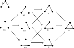
Now set
To define a differential we follow the usual procedure. For a cube edge note that either has the same number of components as or one component less (two components are fused by the additional edge in ). Thus we define to be multiplication in on copies of corresponding to components that fuse (if such exist) and the identity elsewhere. We thus get a complex whose homology is the graph homology of .
Proposition 5.2.2.
Exercise 5.2.3.
Would taking for the differential work as well?
There is a long exact sequence in graph homology which categorifies the deletion-contraction relation. Given an edge we can form two new graphs and where the first has the edge deleted and the second contracts it. There is a short exact sequence
which gives a long exact sequence
5.3. Notes and further reading
The first graph polynomial to be categorified was the chromatic polynomial in [Helme-GuizonRong]. The dichromatic polynomial was studied in [Stǒsić]. Torsion in graph homology has been investigated in [Helme-GuizonPrzytyckiRong].
The reference for Khovanov-Rozansky theory is [KhovanovRozansky1]. While this theory is considerably harder to compute than Khovanov’s original homology some progress has been made. In [Rasmussen3] Rasmussen describes the Khovanov-Rozansky polynomial of 2-bridge knots in terms of the HOMFLYPT polynomial and signature. There is an analogue of Lee’s theory investigated by Gornik in [Gornik]. The polynomial of Murakami, Ohtsuki and Yamada is defined and its properties studied in [MurakamiOhtsukiYamada].
Khovanov and Rozansky followed up their paper with a sequel [KhovanovRozansky2] in which they consider the two variable HOMFLYPT polynomial. Prior to Khovanov and Rozansky’s first paper the case had been treated in a somewhat different manner by Khovanov in [Khovanov5]. Recently, a link with Hochschild homology has been uncovered [Przytycki].
Link diagrams can also be drawn on surfaces and the Jones polynomial can be defined in this context. If the surface is part of the structure then the diagram represents a link in an -bundle over . Khovanov homology in this context has been studied in [AsaedaPrzytyckiSikora]. If the surface is not really part of the structure, but rather just a carrier for the diagram (so you can add/subtract handles away from the diagram) then equivalence classes of diagrams are known as virtual links. Khovanov homology of these has been studied in [Manturov] and [TuraevTurner].
The Jones polynomial corresponds to the 2-dimensional representation of and allowing other representations leads to the coloured Jones polynomial. A link homology theory categorifying this was defined in [Khovanov3].
One of the most interesting questions surrounding the subject is to uncover the geometry that lies behind Khovanov homology. A proposal for a framework unifying Khovanov-Rozansky homology and knot Floer homology has be put forward in [DunfieldGukovRasmussen].
In a different direction P. Seidel and I. Smith have constructed a homology theory for links using symplectic geometry [SeidelSmith]. This theory is conjectured to be isomorphic to Khovanov homology (after suitably collapsing the bi-grading into a single grading). Building on this Manolescu has constructed a similar theory for each and conjectured this to be isomophic to Khovanov-Rozansky homology [Manolescu].
Another exciting direction is to try to give some “physical” interpretation for Khovanov homology (in the sense that Witten gave a physical interpretation of the Jones polynomial as the partition function of a quantum field theory). S. Gukov, A. Schwartz and C. Vafa have made an attempt in this direction [GukovSchwartzVafa] conjecturing a connection to string theory.
Last, but certainly not least, there has been a huge effort to write computer programs to calculate Khovanov homology groups. The first of these by Bar-Natan (using Mathematica) coped with links up to 11 or 12 crossings. This was improved on by Shumakovitch [ShumakovitchKhoHo] with a program using Pari. Bar-Natan now has a nice theoretical trick which speeds things up considerably. This has been implemented by Jeremy Green and you can download the package at from the (wonderful) knot atlas (set up by Dror Bar-Natan and Scott Morrison).
http://katlas.math.toronto.edu/wiki/
Bibliography
- [Abrams] L. Abrams, Two dimensional topological quantum field theories and Frobenius algebras , J. Knot Theory and its Ramifications 5 (1996) 569-587.
- [AsaedaPrzytycki] M. Asaeda and J. Przytycki, Khovanov homology: torsion and thickness, math.GT/0402402.
- [AsaedaPrzytyckiSikora] M. Asaeda, J. Przytycki and A. Sikora, Categorification of the Kauffman bracket skein module of -bundles over surfaces, Alg. Geom. Top., 4 (2004), 1177-1210.
- [Bar-Natan1] D. Bar-Natan, Khovanov’s homology for tangles and cobordisms, Geometry and Topology, 9 (2005), 1443-1499.
- [Bar-Natan2] D. Bar-Natan, On Khovanov’s categorification of the Jones polynomial, Alg. Geom. Top., 2 (2002), 337-370.
- [CarterSaito] J.S. Carter and M. Saito, Knotted surfaces and their diagrams, Mathematical Surveys and Monographs, Vol. 55, AMS 1998.
- [CarterSaitoSatoh] J.S. Carter, M. Saito and S. Satoh, Ribbon-moves for 2-knots with 1-handls attached and Khovanov Jacobsson numbers, math.GT/0407493.
- [DunfieldGukovRasmussen] N. Dunfield, S. Gukov and J. Rasmussen, The superpolynomial for knot homologies, math.GT/0505662.
- [Gornik] B. Gornik, Note on Khovanov link cohomology, math.QA/0402266.
- [GukovSchwartzVafa] S. Gukov, A. Schwartz and C. Vafa, Khovanov-Rozansky homology and topological strings, hep-th/0412243.
- [HeddenOrding] M. Hedden and P. Ording, The Ozsváth-Szabó and Rasmussen concordance invariants are not equal, math.GT/0512348, 2005.
- [Helme-GuizonPrzytyckiRong] L. Helme-Guizon, J. Przytycki and Y. Rong, Torsion in graph homology, math.GT/0507245.
- [Helme-GuizonRong] L. Helme-Guizon and Y. Rong, A categorification for the chromatic polynomial, Alg. Geom. Top, Vol. 5 (2005) 1365-1388.
- [Jacobsson] M. Jacobsson,An invariant of link cobordisms from Khovanov homology, Alg. Geom. Top, Vol. 4 (2004) 1211-1251.
- [Khovanov1] M. Khovanov, A categorification of the Jones polynomial, Duke Math J., 101 (2000), 359-426.
- [Khovanov2] M. Khovanov, A functor valued invariant for tangles, math.GT/0103190.
- [Khovanov3] M. Khovanov, Categorifications of the colored Jones polynomial, math.QA/0302060.
- [Khovanov4] M. Khovanov, Link homology and Frobenius extensions, math.QA/0411447.
- [Khovanov5] M. Khovanov, link homology, Alg. Geom. Top, Vol. 4 (2004) 1045-1081.
- [KhovanovRozansky1] M. Khovanov and L. Rozansky, Matrix factorizations and link homology, math.QA/0401268.
- [KhovanovRozansky2] M. Khovanov and L. Rozansky, Matrix factorizations and link homology II, math.QA/0505056.
- [Kock] J. Kock, Frobenius Algebras and 2-D Topological Quantum Field Theories, LMS Student Texts (No. 59), Cambridge University Press, 2003.
- [KronheimerMrowka] P. Kronheimer and T. Mrowka, Gauge theory for embedded surfaes, I, Topology 32 (1993), 773-826.
- [Lee] E. Lee, An endomorphism of the Khovanov invariant, math.GT/0210213.
- [MackaayTurnerVaz] M. Mackaay, P. Turner and P. Vaz, A remark on Rasmussen’s invariant of knots, math.GT/0509692.
- [Manolescu] C. Manolescu, Link homology theories from symplectic geometry, math.SG/0601629.
- [Manturov] V. Manturov, The Khovanov complex for virtual links, math.GT/0501317.
- [MurakamiOhtsukiYamada] H. Murakami, T. Ohtsuki and S. Yamada, HOMFLY polynomial via an invariant of colored plan graphs, Enseign. Math 44 (1998), 235-360.
- [Przytycki] J. Przytycki, When the theories meet: Khovanov homology as Hochschild homology of links, math.GT/0509334.
- [Rasmussen1] J. Rasmussen, Khovanov homology and the slice genus, math.GT/0402131.
- [Rasmussen2] J. Rasmussen, Khovanov’s invariant for closed surfaces, math.GT/0502527.
- [Rasmussen3] J. Rasmussen, Khovanov-Rozansky homology of two-bridge knots and links, math.GT/0508510.
- [Rasmussen4] J. Rasmussen, Knot polynomials and knot homologies, math.GT/0504045
- [SeidelSmith] P. Seidel and I. Smith, A link invariant from the symplectic geometry of nilpotent slices, math.SG/0405089.
- [Shumakovitch] A. Shumakovitch, Torsion of the Khovanov homology, math.GT/0405474.
- [ShumakovitchKhoHo] A. Shumakovitch, KhoHo: a program for computing Khovanov homology, www.geometrie.ch/KhoHo/
- [Stǒsić] M. Stǒsić, Categorification of the dichromatic polynomial for graphs, math.GT/0504239.
- [Tanaka] K. Tanaka, Khovanov-Jacobsson numbers and invariants of sufrace-knots derived from Bar-Natan’s theory, math.GT/0502371.
- [Turaev] V. Turaev, Quantum invariants of knots and 3-manifolds, de Gruyter Studies in Mathematics, vol. 18, Walter de Gruyter, Berlin, 1994 .
- [TuraevTurner] V. Turaev and P. Turner, Unoriented topological quantum field theory and link homology, math.GT/0506229.
- [Turner] P. Turner, Calculating Bar-Natan’s characteristic two Khovanov homology, math.GT/0411225, 2004.
- [Wehrli] S. Wehrli, Khovanov homology and Conway mutation, math.GT/0301312.
- [Viro] O. Viro, Remarks on the definition of the Khovanov homology, math.GT/0202199.