跳到论文正文
W Papers独立论文阅读器 arXiv:math/0606431 论文正文 计算阅读时间 · 0%
引用这篇论文根据当前论文元数据生成,正式投稿前建议核对。


License: Assumed arXiv.org perpetual non-exclusive license
arXiv:math/0606431v1 [math.OA] 18 Jun 2006

Second Order Freeness
and Fluctuations of Random Matrices:
III. Higher order freeness and free cumulantsThanks: †\dagger Research supported by JSPS and COE postdoctoral fellowshipsThanks: ∗ Research supported by Discovery Grants and a Leadership Support Initiative Award from the Natural Sciences and Engineering Research Council of CanadaThanks: ‡\ddagger Research supported by MNiSW (project 1 P03A 013 30), EU Research Training Network “QP-Applications”, (HPRN-CT-2002-00279) and by European Commission Marie Curie Host Fellowship for the Transfer of Knowledge “Harmonic Analysis, Nonlinear Analysis and Probability” (MTKD-CT-2004-013389).Thanks: {}^{\lx@paragraphsign}\,Research supported by a Premier’s Research Excellence Award from the Province of Ontario and a Killam Fellowship from the Canada Council for the Arts

Benoît Collins † Address: CNRS, Institut Camille Jordan, Université Claude Bernard Lyon 1, 43 boulevard du 11 novembre 1918, 69622 Villeurbanne Cedex, France Email address: collins@math.univ-lyon1.fr , James A. Mingo (∗) Address: Queen’s University, Department of Mathematics and Statistics, Jeffery Hall, Kingston, ON, K7L 3N6, Canada Email address: mingo@mast.queensu.ca , Piotr Śniady (‡) Address: Instytut Matematyczny, Uniwersytet Wroclawski, pl Grunwaldzki 2/4, 50-384 Wroclaw, Poland Email address: Piotr.Sniady@math.uni.wroc.pl and Roland Speicher (∗)(¶) Address: Queen’s University, Department of Mathematics and Statistics, Jeffery Hall, Kingston, ON, K7L 3N6, Canada Email address: speicher@mast.queensu.ca
Abstract.

We extend the relation between random matrices and free probability theory from the level of expectations to the level of all correlation functions (which are classical cumulants of traces of products of the matrices). We introduce the notion of “higher order freeness” and develop a theory of corresponding free cumulants. We show that two independent random matrix ensembles are free of arbitrary order if one of them is unitarily invariant. We prove R-transform formulas for second order freeness. Much of the presented theory relies on a detailed study of the properties of “partitioned permutations”.

1. Introduction

Random matrix models and their large dimension behavior have been an important subject of study in Mathematical Physics and Statistics since Wishart and Wigner. Global fluctuations of the eigenvalues (that is, linear functionals of the eigenvalues) of random matrices have been widely investigated in the last decade; see, e.g., [Joh98, Dia03, Rad04, MN04, MŚS04]. Roughly speaking, the trend of these investigations is that for a wide class of converging random matrix models, the non-normalized trace asymptotically behaves like a Gaussian variable whose variance only depends on macroscopic parameters such as moments. The philosophy of these results, together with the freeness results of Voiculescu served as a motivation for our series of papers on second order freeness.

One of the main achievements of the free probability theory of Voiculescu [Voi91, VDN92] was an abstract description via the notion of “freeness” of the expectation of these Gaussian variables for a large class of non-commuting tuples of random matrices.

In the previous articles of this series [MS04, MŚS04] we showed that for many interesting ensembles of random matrices an analogue of the results of Voiculescu for expectations holds also true on the level of variances as well; thus pointing in the direction that the structure of random matrices and the fine structure of their eigenvalues can be studied in much more detail by using the new concept of “second order freeness”. One of the main obstacles for such a detailed study was the absence of an effective machinery for doing concrete calculations in this framework. Within free probability theory of first order, such a machinery was provided by Voiculescu with the concept of the RR-transform, and by Speicher with the concept of free cumulants; see, e.g., [VDN92, NSp06].

One of the main achievements of the present article is to develop a theory of second order cumulants (and show that the original definition of second order freeness from Part I of this series [MS04] is equivalent to the vanishing of mixed second order cumulants) and provide the corresponding RR-transform machinery.

In Section 2 we will give a more detailed (but still quite condensed) survey of the connection between Voiculescu’s free probability theory and random matrix theory. We will there also provide the main motivation, notions and concepts for our extension of this theory to the level of fluctuations (second order), as well as the statement of our main results concerning second order cumulants and RR-transforms.

Having first and second order freeness it is, of course, a natural question whether this theory can be generalized to higher orders. It turns out that this is the case, most of the general theory is the same for all orders. So we will in this paper consider freeness of all orders from the very beginning and develop a general theory of higher order freeness and higher order cumulants. Let us, however, emphasize that first and second order freeness seem to be more important than the higher order ones. Actually, we can prove some of the most important results (e.g. the RR-transform machinery) only for first and second order, mainly because of the complexity of the underlying combinatorial objects.

The basic combinatorial notion behind the (usual) free cumulants are non-crossing partitions. Basically, passage to higher order free cumulants corresponds to a change to multi-annular non-crossing permutations [MN04], or more general objects which we call “partitioned permutations”. For much of the conceptual framework there is no difference between different levels of freeness, however for many concrete questions it seems that increasing the order makes some calculations much harder. This relates to the fact that nn-th order freeness is described in terms of planar permutations which connect points on nn different circles. Whereas enumeration of all non-crossing permutations in the case of one circle is quite easy, the case of two circles gets more complicated, but is still feasible; for the case of three or more circles, however, the answer does not seem to be of a nice compact form.

In the present paper we develop the notion and combinatorial machinery for freeness of all orders by a careful analysis of the main example: unitarily invariant random matrices. We start with the calculation of mixed correlation functions for random matrices and use the structure which we observe there as a motivation for our combinatorial setup. In this way the concept of partitioned permutations and the moment–cumulant relations appear quite canonically.

We want to point out that even though our notion of second and higher order freeness is modeled on the situation found for correlation functions of random matrices, this notion and theory also have some far-reaching applications. Let us mention in this respect two points.

Firstly, recently one of us [Śni05] developed a quite general theory for fluctuations of characters and shapes of random Young diagrams contributing to many natural representations of symmetric groups. The results presented there are closely (though, not explicitly) related to combinatorics of higher order cumulants. This connection will be studied in detail in the part IV of this series [CMŚS] where we prove that under some mild technical conditions Jucys-Murphy elements, which arise naturally in the study of symmetric groups, are examples of free random variables of higher order.

In another direction, the description of subfactors in von Neumann algebras via planar algebras [Jon99] relies very much on the notions of annular non-crossing partitions and thus resembles the combinatorial objects lying at the basis of our theory of second order freeness. This indicates that our results could have some relevance for subfactors.

Overview of the article

In Section 2 we will give a compact survey of the connection between Voiculescu’s free probability theory and random matrix theory, provide the main motivation, notions and concepts for our extension of this theory to the level of fluctuations (second order), as well as the statement of our main results concerning second order cumulants and RR-transforms. We will also make a few general remarks about higher order freeness.

In Section 3 we will introduce the basic notions and relevant results on permutations, partitions, classical cumulants, Haar unitary random matrices, and the Weingarten function.

In Section 4 we study the correlation functions (classical cumulants of traces) of random matrix models. We will see how those are related to cumulants of entries of the matrices for unitarily invariant random matrices and we will in particular look on the correlation functions for products of two independent ensembles of random matrices, one of which is unitarily invariant. The limit of those formulas if the size NN of the matrices goes to infinity will be the essence of what we are going to call “higher order freeness”. Also our main combinatorial objects, “partitioned permutations”, will arise very naturally in these calculations.

In Section 5 we will forget for a while random variables and just look on the combinatorial essence of our formulas, thus dealing with multiplicative functions on partitioned permutations and their convolution. The Zeta and Möbius functions on partitioned permutations will play an important role in these considerations.

In Section 6 we will derive, for the case of second order, the analogue of the R-transform formulas.

In Section 7 we will finally come back to a (non-commutative) probabilistic context, give the definition and work out the basic properties of “higher order freeness”.

In Section 8 we introduce the notion of “asymptotic higher order freeness”. We show that the Itzykson-Zuber integral encodes all information about higher order freeness. We also indicate how our techniques can give some insight into the computation of some limits of matrix integrals.

In an appendix, Section 9, we provide a graphical interpretation of partitioned permutations as a special case of “surfaced permutations”.

2. Motivation and Statement of our Main Results Concerning Second Order Freeness and Cumulants

In this section we will first recall in a quite compact form the main connection between Voiculescu’s free probability theory and questions about random matrices. Then we want to motivate our notion of second order freeness by extending these questions from the level of expectations to the level of fluctuations. We will recall the relevant results from the papers [MS04, MŚS04] and state the main new results of the present paper. Even though in the later parts of the paper our treatment will include freeness of arbitrarily high order, we restrict ourselves in this section mainly to the second order. The reason for this is that (apart from first order) second order freeness seems to be the most important order for applications, so that it seems worthwhile to spell out our general results for this case more explicitly. Furthermore, it is only there that we have an analogue of RR-transform formulas. We will make a few general remarks about higher order freeness at the end of this section.

2.1. Moments of random matrices and asymptotic freeness

Assume we know the eigenvalue distribution of two matrices AA and BB. What can we say about the eigenvalue distribution of the sum A+BA+B of the matrices? Of course, the latter is not just determined by the eigenvalues of AA and the eigenvalues of BB, but also by the relation between the eigenspaces of AA and of BB. Actually, it is a quite hard problem (Horn’s conjecture) — which was only solved recently — to characterize all possible eigenvalue distributions of A+BA+B. However, if one is asking this question in the context of N×NN\times N-random matrices, then in many situations the answer becomes deterministic in the limit N→∞N\to\infty.

Definition 2.1.

Let A=(AN)N∈ℕA=(A_{N})_{N\in{\mathbb{N}}} be a sequence of N×NN\times N-random matrices. We say that AA has a limit eigenvalue distribution if the limit of all moments

αn:=limN→∞E⁡[tr⁡(ANn)](n∈ℕ)\alpha_{n}:=\lim_{N\to\infty}E[\mathrm{tr}(A_{N}^{n})]\qquad(n\in{\mathbb{N}})

exists, where EE denotes the expectation and tr\mathrm{tr} the normalized trace.

In this language, our question becomes: Given two random matrix ensembles of N×NN\times N-random matrices, A=(AN)N∈ℕA=(A_{N})_{N\in{\mathbb{N}}} and B=(BN)N∈ℕB=(B_{N})_{N\in{\mathbb{N}}}, with limit eigenvalue distribution, does also their sum C=(CN)N∈ℕC=(C_{N})_{N\in{\mathbb{N}}}, with CN=AN+BNC_{N}=A_{N}+B_{N}, have a limit eigenvalue distribution, and furthermore, can we calculate the limit moments αnC\alpha_{n}^{C} of CC out of the limit moments (αkA)k≥1(\alpha_{k}^{A})_{k\geq 1} of AA and the limit moments (αkB)k≥1(\alpha_{k}^{B})_{k\geq 1} of BB in a deterministic way. It turns out that this is the case if the two ensembles are in generic position, and then the rule for calculating the limit moments of CC are given by Voiculescu’s concept of “freeness”. Let us recall this fundamental result of Voiculescu.

Theorem 2.2 (Voiculescu [Voi91]).

Let AA and BB be two random matrix ensembles of N×NN\times N-random matrices, A=(AN)N∈ℕA=(A_{N})_{N\in{\mathbb{N}}} and B=(BN)N∈ℕB=(B_{N})_{N\in{\mathbb{N}}}, each of them with a limit eigenvalue distribution. Assume that AA and BB are independent (i.e., for each N∈ℕN\in{\mathbb{N}}, all entries of ANA_{N} are independent from all entries of BNB_{N}), and that at least one of them is unitarily invariant (i.e., for each NN, the joint distribution of the entries does not change if we conjugate the random matrix with an arbitrary unitary N×NN\times N matrix). Then AA and BB are asymptotically free in the sense of the following definition.

Definition 2.3 (Voiculescu [Voi85]).

Two random matrix ensembles A=(AN)N∈ℕA=(A_{N})_{N\in{\mathbb{N}}} and B=(BN)N∈ℕB=(B_{N})_{N\in{\mathbb{N}}} with limit eigenvalue distributions are asymptotically free if we have for all p≥1p\geq 1 and all n⁡(1),m⁡(1),…,n⁡(p)n(1),m(1),\dots,n(p), m⁡(p)≥1m(p)\geq 1 that

limN→∞E[tr{(ANn⁡(1)−αn⁡(1)A1)⋅(BNm⁡(1)−αm⁡(1)B1)⋯⋯(An⁡(p)−αn⁡(p)A1)⋅(Bm⁡(p)−αm⁡(p)B1)}]=0\lim_{N\to\infty}E\Bigl[\mathrm{tr}\bigl\{(A_{N}^{n(1)}-\alpha_{n(1)}^{A}1)\cdot(B_{N}^{m(1)}-\alpha_{m(1)}^{B}1)\cdots\\ \cdots(A^{n(p)}-\alpha_{n(p)}^{A}1)\cdot(B^{m(p)}-\alpha_{m(p)}^{B}1)\bigr\}\Bigr]=0

One should realize that asymptotic freeness is actually a rule which allows to calculate all mixed moments in AA and BB, i.e. all expressions

limN→∞E[tr(An⁡(1)Bm⁡(1)An⁡(2)Bm⁡(2)⋯An⁡(p)Bm⁡(p))]\lim_{N\to\infty}E[\mathrm{tr}(A^{n(1)}B^{m(1)}A^{n(2)}B^{m(2)}\cdots A^{n(p)}B^{m(p)})]

out of the limit moments of AA and the limit moments of BB. In particular, this means that all limit moments of A+BA+B (which are sums of mixed moments) exist, thus A+BA+B has a limit distribution, and are actually determined in terms of the limit moments of AA and the limit moments of BB. The actual calculation rule is not directly clear from the above definition but a basic result of Voiculescu shows how this can be achieved by going over from the moments αn\alpha_{n} to new quantities κn\kappa_{n}. In [Spe94], the combinatorial structure behind these κn\kappa_{n} was revealed and the name “free cumulants” was coined for them. Whereas in the later parts of this paper we will have to rely crucially on the combinatorial description and their extensions to higher orders, as well as on the definition of more general “mixed” cumulants, we will here state the results in the simplest possible form in terms of generating power series, which avoids the use of combinatorial objects.

Definition 2.4 (Voiculescu [Voi86], Speicher [Spe94]).

Given the moments (αn)n≥1(\alpha_{n})_{n\geq 1} of some distribution (or limit moments of some random matrix ensemble), we define the corresponding free cumulants (κn)n≥1(\kappa_{n})_{n\geq 1} by the following relation between their generating power series: If we put

M⁡(x):=1+∑n≥1αn​xnandC⁡(x):=1+∑n≥1κn​xn,M(x):=1+\sum_{n\geq 1}\alpha_{n}x^{n}\qquad\text{and}\qquad C(x):=1+\sum_{n\geq 1}\kappa_{n}x^{n},

then we require as a relation between these formal power series that

C⁡(x​M​(x))=M⁡(x).C(xM(x))=M(x).

Voiculescu actually formulated the relation above in a slightly different way using the so-called RR-transform ℛ⁡(x)\mathcal{R}(x), which is related to C⁡(x)C(x) by the relation

C⁡(x)=1+z​ℛ​(x)C(x)=1+z\mathcal{R}(x)

and in terms of the Cauchy transform G⁡(x)G(x) corresponding to a measure with moments αn\alpha_{n}, which is related to M⁡(x)M(x) by

G⁡(x)=M⁡(1x)x.G(x)=\frac{M(\frac{1}{x})}{x}.

In these terms the equation C⁡(x​M​(x))=M⁡(x)C(xM(x))=M(x) says that

(1) 1G⁡(x)+ℛ⁡(G⁡(x))=x,\frac{1}{G(x)}+\mathcal{R}(G(x))=x,

i.e., that G⁡(x)G(x) and K⁡(x):=1x+ℛ⁡(x)K(x):=\frac{1}{x}+\mathcal{R}(x) are inverses of each other under composition.

One should also note that the relation C⁡(x​M​(x))=M⁡(x)C(xM(x))=M(x) determines the moments uniquely in terms of the cumulants and the other way around. The relevance of the κn\kappa_{n} and the RR-transform for our problem comes from the following result of Voiculescu, which provides, together with (1), a very efficient way for calculating eigenvalue distributions of the sum of asymptotically free random matrices.

Theorem 2.5 (Voiculescu [Voi86]).

Let AA and BB be two random matrix ensembles which are asymptotically free. Denote by κnA\kappa_{n}^{A}, κnB\kappa_{n}^{B}, κnA+B\kappa_{n}^{A+B} the free cumulants of AA, BB, A+BA+B, respectively. Then one has for all n≥1n\geq 1 that

κnA+B=κnA+κnB.\kappa_{n}^{A+B}=\kappa_{n}^{A}+\kappa_{n}^{B}.

Alternatively,

ℛA+B​(x)=ℛA​(x)+ℛB​(x).\mathcal{R}^{A+B}(x)=\mathcal{R}^{A}(x)+\mathcal{R}^{B}(x).

This theorem is one reason for calling the κn\kappa_{n} cumulants, but there is also another justification for this, namely they are also the limit of classical cumulants of the entries of our random matrix, in the case that this is unitarily invariant. This description will follow from our formulas (28) and (30). We denote the classical cumulants by knk_{n}, considered as multi-linear functionals in nn arguments.

Theorem 2.6.

Let A=(AN)N∈ℕA=(A_{N})_{N\in{\mathbb{N}}} be a unitarily invariant random matrix ensemble of N×NN\times N random matrices ANA_{N} whose limit eigenvalue distribution exists. Then the free cumulants of this matrix ensemble can also be expressed as the limit of special classical cumulants of the entries of the random matrices: If AN=(ai​j(N))i,j=1NA_{N}=(a_{ij}^{(N)})_{i,j=1}^{N}, then

κnA=limN→∞Nn−1​kn​(ai⁡(1)​i​(2)(N),ai⁡(2)​i​(3)(N),…,ai⁡(n),i⁡(1)(N))\kappa_{n}^{A}=\lim_{N\to\infty}N^{n-1}k_{n}(a^{(N)}_{i(1)i(2)},a^{(N)}_{i(2)i(3)},\dots,a^{(N)}_{i(n),i(1)})

for any choice of distinct i⁡(1),…,i⁡(n)i(1),\dots,i(n).

2.2. Fluctuations of random matrices and asymptotic second order freeness

There are many more refined questions about the limiting eigenvalue distribution of random matrices. In particular, questions around fluctuations have received a lot of interest in the last decade or so. The main motivation for introducing the concept of “second order freeness” was to understand the global fluctuations of the eigenvalues, which means that we look at the probabilistic behavior of traces of powers of our matrices. The limiting eigenvalue distribution, as considered in the last section, gives us the limit of the average of this traces. However, one can make more refined statements about their distributions. Consider a random matrix A=(AN)N∈ℕA=(A_{N})_{N\in{\mathbb{N}}} and look on the normalized traces tr⁡(ANk)\mathrm{tr}(A_{N}^{k}). Our assumption of a limit eigenvalue distribution means that the limits αk:=limN→∞E⁡[tr⁡(ANk)]\alpha_{k}:=\lim_{N\to\infty}E[\mathrm{tr}(A_{N}^{k})] exist. It turned out that in many cases the fluctuation around this limit,

tr⁡(ANk)−αk\mathrm{tr}(A_{N}^{k})-\alpha_{k}

is asymptotically Gaussian of order 1/N1/N; i.e., the random variable

N⋅(tr⁡(ANk)−αk)=Tr⁡(ANk)−N​αk=Tr⁡(ANk−αk​1)N\cdot(\mathrm{tr}(A_{N}^{k})-\alpha_{k})=\mathrm{Tr}(A_{N}^{k})-N\alpha_{k}=\mathrm{Tr}(A_{N}^{k}-\alpha_{k}1)

(where Tr\mathrm{Tr} denotes the unnormalized trace) converges for N→∞N\to\infty to a normal variable. Actually, the whole family of centered unnormalized traces (Tr⁡(ANk)−N​αk)k≥1(\mathrm{Tr}(A^{k}_{N})-N\alpha_{k})_{k\geq 1} converges to a centered Gaussian family. (One should note that we restrict all our considerations to complex random matrices; in the case of real random matrices there are additional complications, which will be addressed in some future investigations.) Thus the main information about fluctuations of our considered ensemble is contained in the covariance matrix of the limiting Gaussian family, i.e., in the quantities

αm,n:=limN→∞cov⁡(Tr⁡(ANm),Tr⁡(ANn)).\alpha_{m,n}:=\lim_{N\to\infty}\mathrm{cov}(\mathrm{Tr}(A_{N}^{m}),\mathrm{Tr}(A_{N}^{n})).

Let us emphasize that the αn\alpha_{n} and the αm,n\alpha_{m,n} are actually limits of classical cumulants of traces; for the first and second order, with expectation as first and variance as second cumulant, this might not be so visible, but it will become evident when we go over to higher orders. Nevertheless, the α\alpha’s will behave and will also be treated like moments; accordingly we will call the αm,n\alpha_{m,n} ‘fluctuation moments’. We will later define some other quantities κm,n\kappa_{m,n}, which take the role of cumulants in this context.

This kind of convergence to a Gaussian family was formalized in [MS04] as follows. Note that convergence to Gaussian means that all higher order classical cumulants converge to zero. As before, we denote the classical cumulants by knk_{n}; so k1k_{1} is just the expectation, and k2k_{2} the covariance.

Definition 2.7.

Let A=(AN)N∈ℕA=(A_{N})_{N\in{\mathbb{N}}} be an ensemble of N×NN\times N random matrices ANA_{N}. We say that it has a second order limit distribution if for all m,n≥1m,n\geq 1 the limits

αn:=limN→∞k1​(tr⁡(ANn))\alpha_{n}:=\lim_{N\to\infty}k_{1}(\mathrm{tr}(A_{N}^{n}))

and

αm,n:=limN→∞k2​(Tr⁡(ANm),Tr⁡(ANn))\alpha_{m,n}:=\lim_{N\to\infty}k_{2}(\mathrm{Tr}(A_{N}^{m}),\mathrm{Tr}(A_{N}^{n}))

exist and if

limN→∞kr​(Tr⁡(ANn⁡(1)),…,Tr⁡(ANn⁡(r)))=0\lim_{N\to\infty}k_{r}\bigl(\mathrm{Tr}(A_{N}^{n(1)}),\dots,\mathrm{Tr}(A_{N}^{n(r)})\bigr)=0

for all r≥3r\geq 3 and all n⁡(1),…,n⁡(r)≥1n(1),\dots,n(r)\geq 1.

We can now ask the same kind of question for the limit fluctuations as for the limit moments; namely, if we have two random matrix ensembles AA and BB and we know the second order limit distribution of AA and the second order limit distribution of BB, does this imply that we have a second order limit distribution for A+BA+B, and, if so, is there an effective way for calculating it. Again, we can only hope for a positive solution to this if AA and BB are in a kind of generic position. As it turned out, the same requirements as before are sufficient for this. The rule for calculating mixed fluctuations constitutes the essence of the definition of the concept of second order freeness.

Theorem 2.8 (Mingo, Śniady, Speicher [MŚS04]).

Let AA and BB be two random matrix ensembles of N×NN\times N-random matrices, A=(AN)N∈ℕA=(A_{N})_{N\in{\mathbb{N}}} and B=(BN)N∈ℕB=(B_{N})_{N\in{\mathbb{N}}}, each of them having a second order limit distribution. Assume that AA and BB are independent and that at least one of them is unitarily invariant. Then AA and BB are asymptotically free of second order in the sense of the following definition.

Definition 2.9 (Mingo, Speicher [MS04]).

Consider two random matrix ensembles A=(AN)N∈ℕA=(A_{N})_{N\in{\mathbb{N}}} and B=(BN)N∈ℕB=(B_{N})_{N\in{\mathbb{N}}}, each of them with a second order limit distribution. Denote by

YN​(n⁡(1),m⁡(1),…,n⁡(p),m⁡(p))Y_{N}\bigl(n(1),m(1),\dots,n(p),m(p)\bigr)

the random variable

Tr((ANn⁡(1)−αn⁡(1)A1)(BNm⁡(1)−αm⁡(1)B1)⋯(ANn⁡(p)−αn⁡(p)A1)(BNm⁡(p)−αm⁡(p)B1)).\mathrm{Tr}\bigl((A_{N}^{n(1)}-\alpha_{n(1)}^{A}1)(B_{N}^{m(1)}-\alpha_{m(1)}^{B}1)\cdots(A_{N}^{n(p)}-\alpha^{A}_{n(p)}1)(B_{N}^{m(p)}-\alpha_{m(p)}^{B}1)\bigr).

The random matrices A=(AN)N∈ℕA=(A_{N})_{N\in{\mathbb{N}}} and B=(BN)N∈ℕB=(B_{N})_{N\in{\mathbb{N}}} are asymptotically free of second order if for all n,m≥1n,m\geq 1

limN→∞k2​(Tr⁡(ANn−αnA​1),Tr⁡(BNm−αmB​1))=0\lim_{N\to\infty}k_{2}\bigl(\mathrm{Tr}(A_{N}^{n}-\alpha^{A}_{n}1),\mathrm{Tr}(B_{N}^{m}-\alpha^{B}_{m}1)\bigr)=0

and for all p,q≥1p,q\geq 1 and n⁡(1),…,n⁡(p)n(1),\dots,n(p),m⁡(1),…,m⁡(p)m(1),\dots,m(p),n~​(1),…,n~​(q)\tilde{n}(1),\dots,\tilde{n}(q), m~​(1),…,m~​(q)≥1\tilde{m}(1),\dots,\tilde{m}(q)\geq 1 we have

limN→∞k2​(YN​(n⁡(1),m⁡(1),…,n⁡(p),m⁡(p)),YN​(n~​(1),m~​(2),…,n~​(q),m~​(q)))=0\lim_{N\to\infty}k_{2}\Bigl(Y_{N}\bigl(n(1),m(1),\dots,n(p),m(p)\bigr),Y_{N}\bigl(\tilde{n}(1),\tilde{m}(2),\dots,\tilde{n}(q),\tilde{m}(q)\bigr)\Bigr)=0

if p≠qp\not=q, and otherwise (where we count modulo pp for the arguments of the indices, i.e., n⁡(i+p)=n⁡(i)n(i+p)=n(i))

limN→∞k2​(YN​(n⁡(1),m⁡(1),…,n⁡(p),m⁡(p)),YN​(n~​(p),m~​(p),…,n~​(1),m~​(1)))=∑k=1p∏i=1p(αn​(i+k)+n~​(i)A−αn⁡(i+k)A​αn~​(i)A)​(αm​(i+k)+m~​(i+1)B−αm⁡(i+k)B​αm~​(i+1)B).\lim_{N\to\infty}k_{2}\Bigl(Y_{N}\bigl(n(1),m(1),\dots,n(p),m(p)\bigr),Y_{N}\bigl(\tilde{n}(p),\tilde{m}(p),\dots,\tilde{n}(1),\tilde{m}(1)\bigr)\Bigr)\\ =\sum_{k=1}^{p}\prod_{i=1}^{p}\bigl(\alpha^{A}_{n(i+k)+\tilde{n}(i)}-\alpha^{A}_{n(i+k)}\alpha^{A}_{\tilde{n}(i)}\bigr)\bigl(\alpha^{B}_{m(i+k)+\tilde{m}(i+1)}-\alpha^{B}_{m(i+k)}\alpha^{B}_{\tilde{m}(i+1)}\bigr).

Again, it is crucial to realize that this definition allows one (albeit in a complicated way) to express every second order mixed moment, i.e., a limit of the form

limN→∞k2(Tr(ANn⁡(1)BNm⁡(1)⋯ANn⁡(p)BNm⁡(p)),Tr(ANn~​(1)BNm~​(1)⋯ANn~​(q)BNm~​(q)))\lim_{N\to\infty}k_{2}\bigl(\mathrm{Tr}(A_{N}^{n(1)}B_{N}^{m(1)}\cdots A_{N}^{n(p)}B_{N}^{m(p)}),\mathrm{Tr}(A_{N}^{\tilde{n}(1)}B_{N}^{\tilde{m}(1)}\cdots A_{N}^{\tilde{n}(q)}B_{N}^{\tilde{m}(q)})\bigr)

in terms of the second order limits of AA and the second order limits of BB. In particular, asymptotic freeness of second order also implies that the sum A+BA+B of our random matrix ensembles has a second order limit distribution and allows one to express them in principle in terms of the second order limit distribution of AA and the second order limit distribution of BB. As in the case of first order freeness, it is not clear at all how this calculation of the fluctuations of A+BA+B out of the fluctuations of AA and the fluctuations of BB can be performed effectively. It is one of the main results of the present paper to achieve such an effective description. We are able to solve this problem by providing a second order cumulant machinery, similar to the first order case. Again, the idea is to go over to quantities which behave like cumulants in this setting. The actual description of those relies on combinatorial objects (annular non-crossing permutations), but as before this can be reformulated in terms of formal power series. Let us spell out the definition here in this form. (That this is equivalent to our actual definition of the cumulants will follow from Theorem 6.3.)

Definition 2.10.

Let (αn)n≥1(\alpha_{n})_{n\geq 1} and (αm,n)m,n≥1(\alpha_{m,n})_{m,n\geq 1} describe the first and second order limit moments of a random matrix ensemble. We define the corresponding first and second order free cumulants (κn)n≥1(\kappa_{n})_{n\geq 1} and (κm,n)m,n≥1(\kappa_{m,n})_{m,n\geq 1} by the following requirement in terms of the corresponding generating power series. Put

C⁡(x):=1+∑n≥1κn​xn,C⁡(x,y):=∑m,n≥1κm,n​xm​ynC(x):=1+\sum_{n\geq 1}\kappa_{n}x^{n},\qquad C(x,y):=\sum_{m,n\geq 1}\kappa_{m,n}x^{m}y^{n}

and

M⁡(x):=1+∑n≥1αn​xn,M⁡(x,y):=∑m,n≥1αm,n​xm​yn.M(x):=1+\sum_{n\geq 1}\alpha_{n}x^{n},\qquad M(x,y):=\sum_{m,n\geq 1}\alpha_{m,n}x^{m}y^{n}.

Then we require as relations between these formal power series that

(2) C⁡(x​M​(x))=M⁡(x)C(xM(x))=M(x)

and for the second order

(3) M⁡(x,y)=H⁡(x​M​(x),y​M​(y))⋅dd​x​(x​M​(x))M⁡(x)⋅dd​y​(y​M​(y))M⁡(y),M(x,y)=H\bigl(xM(x),yM(y)\bigr)\cdot\frac{\frac{d}{dx}(xM(x))}{M(x)}\cdot\frac{\frac{d}{dy}(yM(y))}{M(y)},

where

(4) H⁡(x,y):=C⁡(x,y)−x​y​∂2∂x​∂y​log⁡(x​C​(y)−y​C​(x)x−y),H(x,y):=C(x,y)-xy\frac{\partial^{2}}{\partial x\partial y}\log\Bigl(\frac{xC(y)-yC(x)}{x-y}\Bigr),

or equivalently,

(5) M⁡(x,y)=C⁡(x​M​(x),y​M​(y))⋅dd​x​(x​M​(x))M⁡(x)⋅dd​y​(y​M​(y))M⁡(y)+x​y​(dd​x​(x​M​(x))⋅dd​y​(y​M​(y))(x​M​(x)−y​M​(y))2−1(x−y)2).M(x,y)=C\bigl(xM(x),yM(y)\bigr)\cdot\frac{\frac{d}{dx}(xM(x))}{M(x)}\cdot\frac{\frac{d}{dy}(yM(y))}{M(y)}\\ +xy\Bigl(\frac{\frac{d}{dx}(xM(x))\cdot\frac{d}{dy}(yM(y))}{(xM(x)-yM(y))^{2}}-\frac{1}{(x-y)^{2}}\Bigr).

As in the first order case, instead of the moment power series M⁡(x,y)M(x,y) one can consider a kind of second order Cauchy transform, defined by

G⁡(x,y):=M⁡(1x,1y)x​y.G(x,y):=\frac{M(\frac{1}{x},\frac{1}{y})}{xy}.

If we also define a kind of second order RR transform ℛ⁡(x,y)\mathcal{R}(x,y) by

ℛ⁡(x,y):=1x​y​C​(x,y),\mathcal{R}(x,y):=\frac{1}{xy}C(x,y),

then the formula (5) takes on a particularly nice form:

(6) G(x,y)=G′(x)G′(y){ℛ(G(x),G(y))+1(G⁡(x)−G⁡(y))2}−1(x−y)2.G(x,y)=G^{\prime}(x)G^{\prime}(y)\Bigl\{\mathcal{R}(G(x),G(y))+\frac{1}{(G(x)-G(y))^{2}}\Bigl\}-\frac{1}{(x-y)^{2}}.

G⁡(x)G(x) is here, as before, the first order Cauchy transform, G⁡(x)=1x​M​(1/x)G(x)=\frac{1}{x}{M(1/x)}.

The κm,n\kappa_{m,n} defined above deserve the name “cumulants” as they linearize the problem of adding random matrices which are asymptotically free of second order. Namely, as will follow from our Theorem 7.15, we have the following theorem, which provides, together with (6), an effective machinery for calculating the fluctuations of the sum of asymptotically free random matrices.

Theorem 2.11.

Let AA and BB be two random matrix ensembles which are asymptotically free. Then one has for all m,n≥1m,n\geq 1 that

κnA+B=κnA+κnBandκm,nA+B=κm,nA+κm,nB.\kappa_{n}^{A+B}=\kappa_{n}^{A}+\kappa_{n}^{B}\qquad\text{and}\qquad\kappa_{m,n}^{A+B}=\kappa_{m,n}^{A}+\kappa_{m,n}^{B}.

Alternatively,

ℛA+B​(x)=ℛA​(x)+ℛB​(x)\mathcal{R}^{A+B}(x)=\mathcal{R}^{A}(x)+\mathcal{R}^{B}(x)

and

ℛA+B​(x,y)=ℛA​(x,y)+ℛB​(x,y).\mathcal{R}^{A+B}(x,y)=\mathcal{R}^{A}(x,y)+\mathcal{R}^{B}(x,y).

Again, one can express the second order cumulants as limits of classical cumulants of entries of a unitarily invariant matrix. In contrast to the first order case, we have now to run over two disjoint cycles in the indices of the matrix entries. This theorem will follow from our formulas (28) and (30).

Theorem 2.12.

Let A=(AN)N∈ℕA=(A_{N})_{N\in{\mathbb{N}}} be a unitarily invariant random matrix ensemble which has a second order limit distribution. Then the second order free cumulants of this matrix ensemble can also be expressed as the limit of classical cumulants of the entries of the random matrices: If AN=(ai​j(N))i,j=1NA_{N}=(a_{ij}^{(N)})_{i,j=1}^{N}, then

κm,nA=limN→∞Nm+nkm+n(a(N)i⁡(1)​i​(2),a(N)i⁡(2)​i​(3),…,a(N)i⁡(m),i⁡(1),OPENaj⁡(1)​j​(2)(N),aj⁡(2)​j​(3)(N),…,aj⁡(n),j⁡(1)(N))$$\kappa_{m,n}^{A}=\lim_{N\to\infty}N^{m+n}k_{m+n}(a^{(N)}_{i(1)i(2)},a^{(N)}_{i(2)i(3)},\dots,a^{(N)}_{i(m),i(1)},\\ a^{(N)}_{j(1)j(2)},a^{(N)}_{j(2)j(3)},\dots,a^{(N)}_{j(n),j(1)})

for any choice of distinct i⁡(1),…,i⁡(m),j⁡(1),…,j⁡(n)i(1),\dots,i(m),j(1),\dots,j(n).

This latter theorem makes it quite obvious that the second order cumulants for Gaussian as well as for Wishart matrices vanish identically, i.e., ℛ⁡(x,y)=0\mathcal{R}(x,y)=0 and thus we obtain in these cases that the second order Cauchy transform is totally determined in terms of the first order Cauchy transform (i.e., in terms of the limiting eigenvalue distribution) via

(7) G⁡(x,y)=G′​(x)​G′​(y)(G⁡(x)−G⁡(y))2−1(x−y)2.G(x,y)=\frac{G^{\prime}(x)G^{\prime}(y)}{(G(x)-G(y))^{2}}-\frac{1}{(x-y)^{2}}.

This formula for fluctuations of Wishart matrices was also derived by Bai and Silverstein in [BS04].

2.3. Higher order freeness

The idea for higher order freeness is the same as for second order one. For a random matrix ensemble A=(AN)N∈ℕA=(A_{N})_{N\in{\mathbb{N}}} we define rr-th order limit moments as the scaled limit of classical cumulants of rr traces of powers of our matrices,

αn1,…,nr:=limN→∞N2−r​kr​(Tr⁡(ANn⁡(1)),…,Tr⁡(ANn⁡(r))).\alpha_{n_{1},\dots,n_{r}}:=\lim_{N\to\infty}N^{2-r}k_{r}\bigl(\mathrm{Tr}(A_{N}^{n(1)}),\dots,\mathrm{Tr}(A_{N}^{n(r)})\bigr).

(The choice of N2−rN^{2-r} is motivated by the fact that this is the leading order for many interesting random matrix ensembles, e.g. Gaussian or Wishart. Thus our theory of higher order freeness captures the features of random matrix ensembles whose cumulants of traces decay in the same way as for Gaussian random matrices.) Then we look at two random matrix ensembles AA and BB which are independent, and one of them unitarily invariant. The mixed moments in AA and BB of order rr are, in leading order in the limit N→∞N\to\infty, determined by the limit moments of AA up to order rr and the limit moments of BB up to order rr. The structure of these formulas motivates directly the definition of cumulants of the considered order. The definition of those is in terms of a moment-cumulant formula, which gives a moment in terms of cumulants by summing over special combinatorial objects, which we call “partitioned permutations”. Most of the theory we develop relies on an in depth analysis of properties of these partitioned permutations and the corresponding convolution of multiplicative functions on partitioned permutations. Our definition of “higher order freeness” is then in terms of the vanishing of mixed cumulants. It follows quite easily that in the first and second order case this gives the same as the relations in Definitions 2.3 and 2.9, respectively. For higher orders, however, we are not able to find an explicit relation of that type.

This reflects somehow the observation that our general formulas in terms of sums over partitioned permutations are the same for all orders, but that evaluating or simplifying these sums (by doing partial summations) is beyond our abilities for orders greater than 2. Reformulating the combinatorial relation between moments and cumulants in terms of generating power series is one prominent example for this. Whereas this is quite easy for first order, the complexity of the arguments and the solution (given in Definition 2.10) is much higher for second order, and out of reach for higher order.

One should note that an effective (analytic or symbolic) calculation of higher order moments of a sum A+BA+B for AA and BB free of higher order relies usually on the presence of such generating power series formulas. In this sense, we have succeeded in providing an effective machinery for dealing with fluctuations (second order), but we were not able to do so for higher order.

Our results for higher orders are more of a theoretical nature. One of the main problems we have to address there is the associativity of the notion of higher order freeness. Namely, in order to be an interesting concept, our definition that AA and BB are free of higher order should of course imply that any function of AA is also free of higher order from any function of BB. Whereas for first and second order this follows quite easily from the equivalent characterization of freeness in terms of moments as in Definitions 2.3 and 2.9, the absence of such a characterization for higher orders makes this a more complicated matter. Namely, what we have to see is that the vanishing of mixed cumulants in random variables implies also the vanishing of mixed cumulants in elements from the generated algebras. This is a quite non-trivial fact and requires a careful analysis, see section 7.

3. Preliminaries

3.1. Some general notation

For natural numbers m,n∈ℕm,n\in{\mathbb{N}} with m<nm<n, we denote by [m,n][m,n] the interval of natural numbers between mm and nn, i.e.,

[m,n]:={m,m+1,m+2,…,n−1,n}.[m,n]:=\{m,m+1,m+2,\dots,n-1,n\}.

For a matrix A=(ai​j)i,j=1NA=(a_{ij})_{i,j=1}^{N}, we denote by Tr\mathrm{Tr} the unnormalized and by tr\mathrm{tr} the normalized trace,

Tr⁡(A):=∑i=1Nai​i,tr⁡(A):=1N​Tr​(A).\mathrm{Tr}(A):=\sum_{i=1}^{N}a_{ii},\qquad\mathrm{tr}(A):=\frac{1}{N}\mathrm{Tr}(A).

3.2. Permutations

We will denote the set of permutations on nn elements by SnS_{n}. We will quite often use the cycle notation for such permutations, i.e., π=(i1,i2,…,ir)\pi=(i_{1},i_{2},\dots,i_{r}) is a cycle which sends iki_{k} to ik+1i_{k+1} (k=1,…,rk=1,\dots,r), where ir+1=i1i_{r+1}=i_{1}.

3.2.1. Length function

For a permutation π∈Sn\pi\in S_{n} we denote by #​π\#\pi the number of cycles of π\pi and by |π||\pi| the minimal number of transpositions needed to write π\pi as a product of transpositions. Note that one has

|π|+#​π=nfor all π∈Sn.|\pi|+\#\pi=n\qquad\text{for all $\pi\in S_{n}$}.

3.2.2. Non-crossing permutations

Let us denote by γn∈Sn\gamma_{n}\in S_{n} the cycle

γn=(1,2,…,n).\gamma_{n}=(1,2,\dots,n).

For all π∈Sn\pi\in S_{n} one has that

|π|+|γn​π−1|≤n−1.|\pi|+|\gamma_{n}\pi^{-1}|\leq n-1.

If we have equality then we call π\pi non-crossing. Note that this is equivalent to

#​π+#⁡(γn​π−1)=n+1.\#\pi+\#(\gamma_{n}\pi^{-1})=n+1.

If π\pi is non-crossing, then so are γn​π−1\gamma_{n}\pi^{-1} and π−1​γn\pi^{-1}\gamma_{n}; the latter is called the (Kreweras) complement of π\pi.

We will denote the set of non-crossing permutations in SnS_{n} by N​C​(n)NC(n). Note that such a non-crossing permutation can be identified with a non-crossing partition, by forgetting the order on the cycles. There is exactly one cyclic order on the blocks of a non-crossing partition which makes it into a non-crossing permutation.

3.2.3. Annular non-crossing permutations

Fix m,n∈ℕm,n\in{\mathbb{N}} and denote by γm,n\gamma_{m,n} the product of the two cycles

γm,n=(1,2,…,m)​(m+1,m+2,…,m+n).\gamma_{m,n}=(1,2,\dots,m)(m+1,m+2,\dots,m+n).

More generally, we shall denote by γm1,…,mk\gamma_{m_{1},\dots,m_{k}} the product of the corresponding kk cycles.

We call a π∈Sm+n\pi\in S_{m+n} connected if the pair π\pi and γm,n\gamma_{m,n} generates a transitive subgroup in Sm+nS_{m+n}. A connected permutation π∈Sm+n\pi\in S_{m+n} always satisfies

(8) |π|+|γm,n​π−1|≤m+n.|\pi|+|\gamma_{m,n}\pi^{-1}|\leq m+n.

If π\pi is connected and if we have equality in that equation then we call π\pi annular non-crossing. Note that if π\pi is annular non-crossing then γm,n​π−1\gamma_{m,n}\pi^{-1} is also annular non-crossing. Again, we call the latter the complement of π\pi. Of course, all the above notations depend on the pair (m,n)(m,n); if we want to emphasize this dependency we will also speak about (m,n)(m,n)-connected permutations and (m,n)(m,n)-annular non-crossing permutations.

We will denote the set of (m,n)(m,n)-annular non-crossing permutations by SN​C​(m,n)S_{NC}(m,n). A cycle of a π∈SN​C​(m,n)\pi\in S_{NC}(m,n) is called a through-cycle if it contains points on both cycles. Each π∈SN​C​(m,n)\pi\in S_{NC}(m,n) is connected and must thus have at least one through-cycle. The subset of SN​C​(m,n)S_{NC}(m,n) where all cycles are through-cycles will be denoted by SN​Ca​l​l​(m,n)S_{NC}^{all}(m,n).

Again one can go over from annular non-crossing permutations to annular non-crossing partitions by forgetting the cyclic orders on cycles; however, in the annular case, the relation between non-crossing permutation and non-crossing partition is not one-to-one. Since we will not use the language of annular partitions in the present paper, this is of no relevance here.

Annular non-crossing permutations and partitions were introduced in [MN04]; there, many different characterizations—in particular, the one (8) above in terms of the length function—were given.

3.3. Partitions

We say that 𝒱={V1,…,Vk}{\mathcal{V}}=\{V_{1},\dots,V_{k}\} is a partition of a set [1,n][1,n] if the sets ViV_{i} are disjoint and non–empty and their union is equal to [1,n][1,n]. We call V1,…,VkV_{1},\dots,V_{k} the blocks of partition 𝒱{\mathcal{V}}.

If 𝒱={V1,…,Vk}{\mathcal{V}}=\{V_{1},\dots,V_{k}\} and 𝒲={W1,…,Wl}{\mathcal{W}}=\{W_{1},\dots,W_{l}\} are partitions of the same set, we say that 𝒱≤𝒲{\mathcal{V}}\leq{\mathcal{W}} if for every block ViV_{i} there exists some block WjW_{j} such that Vi⊆WjV_{i}\subseteq W_{j}. For a pair of partitions 𝒱,𝒲{\mathcal{V}},{\mathcal{W}} we denote by 𝒱∨𝒲{\mathcal{V}}\vee{\mathcal{W}} the smallest partition 𝒰{\mathcal{U}} such that 𝒱≤𝒰{\mathcal{V}}\leq{\mathcal{U}} and 𝒲≤𝒰{\mathcal{W}}\leq{\mathcal{U}}. We denote by 1n={[1,n]}1_{n}=\big\{[1,n]\big\} the biggest partition of the set [1,n][1,n].

If π∈Sn\pi\in S_{n} is a permutation, then we can associate to π\pi in a natural way a partition whose blocks consist exactly of the cycles of π\pi; we will denote this partition either by 0π∈𝒫⁡(n)0_{\pi}\in{\mathcal{P}}(n) or, if the context makes the meaning clear, just by π∈𝒫⁡(n)\pi\in{\mathcal{P}}(n).

For a permutation π∈Sn\pi\in S_{n} we say that a partition 𝒱{\mathcal{V}} is π\pi-invariant if π\pi preserves each block of 𝒱{\mathcal{V}}. This means that 0π≤𝒱0_{\pi}\leq{\mathcal{V}} (which we will usually write just as π≤𝒱\pi\leq{\mathcal{V}}).

If 𝒱={V1,…,Vk}{\mathcal{V}}=\{V_{1},\dots,V_{k}\} is a partition of the set [1,n][1,n] and if, for 1≤i≤k1\leq i\leq k, πi\pi_{i} is a permutation of the set ViV_{i} we denote by π1×⋯×πk∈Sn\pi_{1}\times\cdots\times\pi_{k}\in S_{n} the concatenation of these permutations. We say that π=π1×⋯×πk\pi=\pi_{1}\times\cdots\times\pi_{k} is a cycle decomposition if additionally every factor πi\pi_{i} is a cycle.

3.4. Classical cumulants

Given some classical probability space (Ω,P)(\Omega,\allowbreak P) we denote by E\mathrm{E} the expectation with respect to the corresponding probability measure,

E⁡(a):=∫Ωa⁡(ω)​𝑑P​(ω)\mathrm{E}(a):=\int_{\Omega}a(\omega)dP(\omega)

and by L∞−​(Ω,P)L^{\infty-}(\Omega,P) the algebra of random variables for which all moments exist. Let us for the following put 𝒜:=L∞−​(Ω,P)\mathcal{A}:=L^{\infty-}(\Omega,P).

We extend the linear functional E:𝒜→ℂ\mathrm{E}:\mathcal{A}\to{\mathbb{C}} to a corresponding multiplicative functional on all partitions by (𝒱∈𝒫⁡(n){\mathcal{V}}\in{\mathcal{P}}(n), a1,…,an∈𝒜a_{1},\dots,a_{n}\in\mathcal{A})

(9) E𝒱​[a1,…,an]:=∏V∈𝒱E⁡[a1,…,an|V],\mathrm{E}_{\mathcal{V}}[a_{1},\dots,a_{n}]:=\prod_{V\in{\mathcal{V}}}\mathrm{E}[a_{1},\dots,a_{n}|_{V}],

where we use the notation

E[a1,…,an|V]:=E(ai1⋯ais)forV=(i1<⋯<is)∈𝒱.\mathrm{E}[a_{1},\dots,a_{n}|_{V}]:=\mathrm{E}(a_{i_{1}}\cdots a_{i_{s}})\qquad\text{for}\qquad V=(i_{1}<\dots<i_{s})\in{\mathcal{V}}.

Then, for 𝒱∈𝒫⁡(n){\mathcal{V}}\in{\mathcal{P}}(n), we define the classical cumulants k𝒱k_{\mathcal{V}} as multilinear functionals on 𝒜\mathcal{A} by

(10) k𝒱​[a1,…,an]=∑𝒲∈𝒫⁡(n)𝒲≤𝒱E𝒲​[a1,…,an]⋅Möb𝒫⁡(n)​(𝒲,𝒱),k_{\mathcal{V}}[a_{1},\dots,a_{n}]=\sum_{{\mathcal{W}}\in{\mathcal{P}}(n)\atop{\mathcal{W}}\leq{\mathcal{V}}}\mathrm{E}_{\mathcal{W}}[a_{1},\dots,a_{n}]\cdot\mathrm{\text{M\"{o}b}}_{{\mathcal{P}}(n)}({\mathcal{W}},{\mathcal{V}}),

where Möb𝒫⁡(n)\mathrm{\text{M\"{o}b}}_{{\mathcal{P}}(n)} denotes the Möbius function on 𝒫⁡(n){\mathcal{P}}(n) (see [Rot64]).

The above definition is, by Möbius inversion on 𝒫⁡(n){\mathcal{P}}(n), equivalent to

E(a1⋯an)=∑π∈𝒫⁡(n)kπ[a1,…,an].\mathrm{E}(a_{1}\cdots a_{n})=\sum_{\pi\in{\mathcal{P}}(n)}k_{\pi}[a_{1},\dots,a_{n}].

The kπk_{\pi} are also multiplicative with respect to the blocks of 𝒱{\mathcal{V}} and thus determined by the values of

kn​(a1,…,an):=k1n​[a1,…,an].k_{n}(a_{1},\dots,a_{n}):=k_{1_{n}}[a_{1},\dots,a_{n}].

Note that we have in particular

k1​(a)=E⁡(a)andk2​(a1,a2)=E⁡(a1​a2)−E⁡(a1)​E​(a2).k_{1}(a)=\mathrm{E}(a)\qquad\text{and}\qquad k_{2}(a_{1},a_{2})=\mathrm{E}(a_{1}a_{2})-\mathrm{E}(a_{1})\mathrm{E}(a_{2}).

An important property of classical cumulants is the following formula of Leonov and Shiryaev [LS59] for cumulants with products as arguments.

Let m,n∈ℕm,n\in{\mathbb{N}} and 1≤i⁡(1)<i⁡(2)<⋯<i⁡(m)=n1\leq i(1)<i(2)<\cdots<i(m)=n. Define 𝒰∈𝒫⁡(n){\mathcal{U}}\in{\mathcal{P}}(n) by

𝒰={(1,…,i⁡(1)),(i⁡(i)+1,…,i⁡(2)),…,(i⁡(m−1)+1,…,i⁡(m))}.{\mathcal{U}}=\bigl\{\bigl(1,\dots,i(1)\bigr),\bigl(i(i)+1,\dots,i(2)\bigr),\dots,\bigl({i({m-1})+1},\dots,i(m)\bigr)\bigr\}.

Consider now random variables a1,…,an∈𝒜a_{1},\dots,a_{n}\in\mathcal{A} and define

A1:\displaystyle A_{1}: =a1⋯ai⁡(1)\displaystyle=a_{1}\cdots a_{i(1)}
A2:\displaystyle A_{2}: =ai⁡(1)+1⋯ai⁡(2)\displaystyle=a_{i(1)+1}\cdots a_{i(2)}
Am:\displaystyle A_{m}: =ai⁡(m−1)+1⋯ai⁡(m).\displaystyle=a_{i({m-1})+1}\cdots a_{i(m)}.

Then we have

(11) km​(A1,A2,…,Am)=∑𝒱∈𝒫⁡(n)𝒱∨𝒰=1nk𝒱​[a1,…,an].k_{m}(A_{1},A_{2},\dots,A_{m})=\sum_{{\mathcal{V}}\in{\mathcal{P}}(n)\atop{\mathcal{V}}\vee{\mathcal{U}}=1_{n}}k_{{\mathcal{V}}}[a_{1},\dots,a_{n}].

The sum on the right-hand side is running over those partitions of nn elements which satisfy 𝒱∨𝒰=1n{\mathcal{V}}\vee{\mathcal{U}}=1_{n}, which are, informally speaking, those partitions which connect all the arguments of the cumulant kmk_{m}, when written in terms of the aia_{i}.

Here is an example for this formula; for k2​(a1​a2,a3​a4)k_{2}(a_{1}a_{2},a_{3}a_{4}). In order to reduce the number of involved terms we will restrict to the special case where E⁡(ai)=0\mathrm{E}(a_{i})=0 (and thus also k1​(ai)=0k_{1}(a_{i})=0) for all i=1,2,3,4i=1,2,3,4. There are three partitions π∈𝒫⁡(4)\pi\in{\mathcal{P}}(4) without singletons which satisfy

π∨{(1,2),(3,4)}=14,\pi\vee\{(1,2),(3,4)\}=1_{4},

namely

and thus formula (11) gives in this case

k2​(a1​a2,a3​a4)=k4​(a1,a2,a3,a4)+k2​(a1,a4)​k2​(a2,a3)+k2​(a1,a3)​k2​(a2,a4).k_{2}(a_{1}a_{2},a_{3}a_{4})=k_{4}(a_{1},a_{2},a_{3},a_{4})\\ +k_{2}(a_{1},a_{4})k_{2}(a_{2},a_{3})+k_{2}(a_{1},a_{3})k_{2}(a_{2},a_{4}).

As a consequence of (11) one has the following important corollary: If {a1,…,an}\{a_{1},\dots,a_{n}\} and {b1,…,bn}\{b_{1},\dots,b_{n}\} are independent then

(12) k𝒲​[a1​b1,…,an​bn]=∑𝒱,𝒱′∈𝒫⁡(n)𝒱∨𝒱′=𝒲k𝒱​[a1,…,an]⋅k𝒱′​[b1,…,bn].k_{\mathcal{W}}[a_{1}b_{1},\dots,a_{n}b_{n}]=\sum_{{\mathcal{V}},{\mathcal{V}}^{\prime}\in{\mathcal{P}}(n)\atop{\mathcal{V}}\vee{\mathcal{V}}^{\prime}={\mathcal{W}}}k_{{\mathcal{V}}}[a_{1},\dots,a_{n}]\cdot k_{{\mathcal{V}}^{\prime}}[b_{1},\dots,b_{n}].

3.5. Haar distributed unitary random matrices and the Weingarten function

In the following we will be interested in the asymptotics of special matrix integrals over the group 𝒰⁡(N)\mathcal{U}(N) of unitary N×NN\times N-matrices. We always equip the compact group 𝒰⁡(N)\mathcal{U}(N) with its Haar probability measure. A random matrix whose distribution is this measure will be called a Haar distributed unitary random matrix. Thus the expectation E\mathrm{E} over this ensemble is given by integrating with respect to the Haar measure.

The expectation of products of entries of Haar distributed unitary random matrices can be described in terms of a special function on the permutation group. Since such considerations go back to Weingarten [Wei78], Collins [Col03] calls this function the Weingarten function and denotes it by Wg\mathrm{Wg}. We will follow his notation. In the following we just recall the relevant information about this Weingarten function, for more details we refer to [Col03, CŚ04].

We use the following definition of the Weingarten function. For π∈Sn\pi\in S_{n} and N≥nN\geq n we put

Wg(N,π)=E[u11⋯un​nu1​π​(1)¯⋯un​π​(n)¯],\mathrm{Wg}(N,\pi)=\mathrm{E}[u_{11}\cdots u_{nn}\overline{u_{1\pi(1)}}\cdots\overline{u_{n\pi(n)}}],

where U=(ui​j)i,j=1NU=(u_{ij})_{i,j=1}^{N} is an N×NN\times N Haar distributed unitary random matrix. Sometimes we will suppress the dependency on NN and just write Wg⁡(π)\mathrm{Wg}(\pi). This Wg⁡(N,π)\mathrm{Wg}(N,\pi) depends only on the conjugacy class of π\pi. General matrix integrals over the unitary group can be calculated as follows:

(13) E[ui1′​j1′⋯uin′​jn′ui1​j1¯⋯uin​jn¯]=∑α,β∈Snδi1​iα⁡(1)′⋯δin​iα⁡(n)′δj1​jβ⁡(1)′⋯δjn​jβ⁡(n)′Wg(βα−1).\mathrm{E}[u_{i^{\prime}_{1}j^{\prime}_{1}}\cdots u_{i^{\prime}_{n}j^{\prime}_{n}}\overline{u_{i_{1}j_{1}}}\cdots\overline{u_{i_{n}j_{n}}}]\\ =\sum_{\alpha,\beta\in S_{n}}\delta_{i_{1}i^{\prime}_{\alpha(1)}}\cdots\delta_{i_{n}i^{\prime}_{\alpha(n)}}\delta_{j_{1}j^{\prime}_{\beta(1)}}\cdots\delta_{j_{n}j^{\prime}_{\beta(n)}}\mathrm{Wg}(\beta\alpha^{-1}).

This formula for the calculation of moments of the entries of a Haar unitary random matrix bears some resemblance to the Wick formula for the joint moments of the entries of Gaussian random matrices; thus we will call (13) the Wick formula for Haar unitary matrices.

The Weingarten function is quite a complicated object, and its full understanding is at the basis of questions around Itzykson-Zuber integrals. One knows (see, e.g., [Col03, CŚ04]) that the leading order in 1/N1/N is given by |π|+n|\pi|+n and increases in steps of 2.

3.6. Cumulants of the Weingarten function

We will also need some (classical) relative cumulants of the Weingarten function, which were introduced in [Col03, §2.3]. As before, let Möb𝒫⁡(n)\mathrm{\text{M\"{o}b}}_{{\mathcal{P}}(n)} be the Möbius function on the partially ordered set of partitions of [1,n][1,n] ordered by inclusion.

Let us first extend the Weingarten function by multiplicative extension, for 𝒱≥π{\mathcal{V}}\geq\pi, by

Wg⁡(𝒱,π):=∏V∈𝒱Wg⁡(π|V),\mathrm{Wg}({\mathcal{V}},\pi):=\prod_{V\in{\mathcal{V}}}\mathrm{Wg}(\pi|_{V}),

where π|V\pi|_{V} denotes the restriction of π\pi to the block V∈𝒱V\in{\mathcal{V}} (which is invariant under π\pi since π≤𝒱\pi\leq{\mathcal{V}}).

The relative cumulant of the Weingarten function is now, for σ≤𝒱≤𝒲\sigma\leq{\mathcal{V}}\leq{\mathcal{W}}, defined by

(14) C𝒱,𝒲​(σ)=∑𝒰∈𝒫⁡(n)𝒱≤𝒰≤𝒲Möb​(𝒰,𝒲)⋅Wg⁡(𝒰,σ)C_{{\mathcal{V}},{\mathcal{W}}}(\sigma)=\sum_{{\mathcal{U}}\in{\mathcal{P}}(n)\atop{\mathcal{V}}\leq{\mathcal{U}}\leq{\mathcal{W}}}\mathrm{\text{M\"{o}b}}({\mathcal{U}},{\mathcal{W}})\cdot\mathrm{Wg}({\mathcal{U}},\sigma)

Note that, by Möbius inversion, this is, for any σ≤𝒱≤𝒲\sigma\leq{\mathcal{V}}\leq{\mathcal{W}}, equivalent to

(15) Wg⁡(𝒲,σ)=∑𝒰∈𝒫⁡(n)𝒱≤𝒰≤𝒲C𝒱,𝒰​(σ).\mathrm{Wg}({\mathcal{W}},\sigma)=\sum_{{\mathcal{U}}\in{\mathcal{P}}(n)\atop{\mathcal{V}}\leq{\mathcal{U}}\leq{\mathcal{W}}}C_{{\mathcal{V}},{\mathcal{U}}}(\sigma).

In [Col03, Cor. 2.9] it was shown that the order of C𝒱,𝒲​(σ)C_{{\mathcal{V}},{\mathcal{W}}}(\sigma) is at most

(16) N−2​n+#​σ+2​#​𝒲−2​#​𝒱.N^{-2n+\#\sigma+2\#{\mathcal{W}}-2\#{\mathcal{V}}}.

4. Correlation functions for random matrices

4.1. Correlation functions and partitioned permutations

Let us consider N×NN\times N-random matrices B1,…,Bn:Ω→MN​(ℂ)B_{1},\dots,B_{n}:\Omega\to M_{N}({\mathbb{C}}). The main information we are interested in are the “correlation functions” φn\varphi_{n} of these matrices, given by classical cumulants of their traces, i.e.,

φn​(B1,…,Bn):=kn​(Tr⁡(B1),…,Tr⁡(Bn)).\varphi_{n}(B_{1},\dots,B_{n}):=k_{n}(\mathrm{Tr}(B_{1}),\dots,\mathrm{Tr}(B_{n})).

Even though these correlation functions are cumulants, it is more adequate to consider them as a kind of moments for our random matrices. Thus, we will also call them sometimes correlation moments.

We will also need to consider traces of products which are best encoded via permutations. Thus, for π∈Sn\pi\in S_{n}, φ⁡(π)​[B1,…,Bn]\varphi(\pi)[B_{1},\dots,B_{n}] shall mean that we take cumulants of traces of products along the cycles of π\pi. For an nn-tuple B=(B1,…,Bn)B=(B_{1},\dots,B_{n}) of random matrices and a cycle c=(i1,i2,…,ik)c=(i_{1},i_{2},\dots,i_{k}) with k≤nk\leq n we denote

B|c:=Bi1Bi2⋯Bik.B|_{c}:=B_{i_{1}}B_{i_{2}}\cdots B_{i_{k}}.

(We do not distinguish between products which differ by a cyclic rotation of the factors; however, in order to make this definition well-defined we could normalize our cycle c=(i1,i2,…,ik)c=(i_{1},i_{2},\dots,i_{k}) by the requirement that i1i_{1} is the smallest among the appearing numbers.) For any π∈S⁡(n)\pi\in S(n) and any nn-tuple B=(B1,…,Bn)B=(B_{1},\dots,B_{n}) of random matrices we put

φ⁡(π)​[B1,…,Bn]:=φr​(B|c1,…,B|cr),\varphi(\pi)[B_{1},\dots,B_{n}]:=\varphi_{r}(B|_{c_{1}},\dots,B|_{c_{r}}),

where π\pi consists of the cycles c1,…,crc_{1},\dots,c_{r}.

Example:

φ⁡((1,3)​(2,5,4))​[B1,B2,B3,B4,B5]\displaystyle\varphi((1,3)(2,5,4))[B_{1},B_{2},B_{3},B_{4},B_{5}] =φ2​(B1​B3,B2​B5​B4)\displaystyle=\varphi_{2}(B_{1}B_{3},B_{2}B_{5}B_{4})
=k2​(Tr⁡(B1​B3),Tr⁡(B2​B5​B4))\displaystyle=k_{2}(\mathrm{Tr}(B_{1}B_{3}),\mathrm{Tr}(B_{2}B_{5}B_{4}))

Furthermore, we also need to consider more general products of such φ⁡(π)\varphi(\pi)’s. In order to index such products we will use pairs (𝒱,π)({\mathcal{V}},\pi) where π\pi is, as above, an element in SnS_{n}, and 𝒱∈𝒫⁡(n){\mathcal{V}}\in{\mathcal{P}}(n) is a partition which is compatible with the cycle structure of π\pi, i.e., each block of 𝒱{\mathcal{V}} is fixed under π\pi, or to put it another way, 𝒱≥π{\mathcal{V}}\geq\pi. In the latter inequality we use the convention that we identify a permutation with the partition corresponding to its cycles if this identification is obvious from the structure of the formula; we will write this partition 0π0_{\pi} or just 0 if no confusion will result.

Notation 4.1.

A partitioned permutation is a pair (𝒱,π)({\mathcal{V}},\pi) consisting of π∈Sn\pi\in S_{n} and 𝒱∈𝒫⁡(n){\mathcal{V}}\in{\mathcal{P}}(n) with 𝒱≥π{\mathcal{V}}\geq\pi. We will denote the set of partitioned permutations of nn elements by 𝒫​𝒮​(n){\mathcal{PS}}(n). We will also put

𝒫​𝒮:=⋃n∈ℕ𝒫​𝒮​(n).{\mathcal{PS}}:=\bigcup_{n\in{\mathbb{N}}}{\mathcal{PS}}(n).

For such a (𝒱,π)∈𝒫​𝒮({\mathcal{V}},\pi)\in{\mathcal{PS}} we denote finally

φ⁡(𝒱,π)​[B1,…,Bn]:=∏V∈𝒱φ⁡(π|V)​[B1,…,Bn|V].\varphi({\mathcal{V}},\pi)[B_{1},\dots,B_{n}]:=\prod_{V\in{\mathcal{V}}}\varphi(\pi|_{V})[B_{1},\dots,B_{n}|_{V}].

Example:

φ⁡({1,3,4}​{2},(1,3)​(2)​(4))\displaystyle\varphi\bigl(\{1,3,4\}\{2\},(1,3)(2)(4)\bigr) [B1,B2,B3,B4]\displaystyle[B_{1},B_{2},B_{3},B_{4}]
=φ2​(B1​B3,B4)⋅φ1​(B2)\displaystyle=\varphi_{2}(B_{1}B_{3},B_{4})\cdot\varphi_{1}(B_{2})
=k2​(Tr⁡(B1​B3),Tr⁡(B4))⋅k1​(Tr⁡(B2))\displaystyle=k_{2}(\mathrm{Tr}(B_{1}B_{3}),\mathrm{Tr}(B_{4}))\cdot k_{1}(\mathrm{Tr}(B_{2}))

Let us denote by Trσ\mathrm{Tr}_{\sigma} as usual a product of traces along the cycles of σ\sigma. Then we have the relation

E⁡{Trσ​[A1,…,An]}=∑𝒲∈𝒫⁡(n)𝒲≥σφ⁡(𝒲,σ)​[A1,…,An].\mathrm{E}\{\mathrm{Tr}_{\sigma}[A_{1},\dots,A_{n}]\}=\sum_{{\mathcal{W}}\in{\mathcal{P}}(n)\atop{\mathcal{W}}\geq\sigma}\varphi({\mathcal{W}},\sigma)[A_{1},\dots,A_{n}].

By using the formula (11) of Leonov and Shiryaev one sees that in terms of the entries of our matrices Bk=(bi​j(k))i,j=1NB_{k}=(b_{ij}^{(k)})_{i,j=1}^{N} our φ⁡(𝒰,γ)\varphi({\mathcal{U}},\gamma) can also be written as

(17) φ⁡(𝒰,γ)​[B1,…,Bn]=∑𝒱≤𝒰𝒱∨γ=𝒰∑i⁡(1),…,i⁡(n)=1Nk𝒱​[bi⁡(1)​i​(γ⁡(1))(1),…,bi⁡(n)​i​(γ⁡(n))(n)].\varphi({\mathcal{U}},\gamma)[B_{1},\dots,B_{n}]=\sum_{{\mathcal{V}}\leq{\mathcal{U}}\atop{\mathcal{V}}\vee\gamma={\mathcal{U}}}\sum_{i(1),\dots,i(n)=1}^{N}k_{\mathcal{V}}[b_{i(1)i(\gamma(1))}^{(1)},\dots,b_{i(n)i(\gamma(n))}^{(n)}].

4.2. Moments of unitarily invariant random matrices

For unitarily invariant random matrices there exists a definite relation between cumulants of traces and cumulants of entries. We want to work out this connection in this section.

Definition 4.2.

Random matrices A1,…,AnA_{1},\dots,A_{n} are called unitarily invariant if the joint distribution of all their entries does not change by global conjugation with any unitary matrix, i.e., if, for any unitary matrix UU, the matrix-valued random variables A1,…,An:Ω→MN​(ℂ)A_{1},\dots,A_{n}:\Omega\to M_{N}({\mathbb{C}}) have the same joint distribution as the matrix-valued random variables U​A1​U∗,…,U​An​U∗:Ω→MN​(ℂ)UA_{1}U^{*},\dots,UA_{n}U^{*}:\Omega\to M_{N}({\mathbb{C}}).

Let A1,…,AnA_{1},\dots,A_{n} be unitarily invariant random matrices. We will now try expressing the microscopic quantities “cumulants of entries of the AiA_{i}” in terms of the macroscopic quantities “cumulants of traces of products of the AiA_{i}”.

In order to make this connection we have to use the unitary invariance of our ensemble. By definition, this means that A1,…,AnA_{1},\dots,A_{n} has the same distribution as A~1,…,A~n\tilde{A}_{1},\dots,\tilde{A}_{n} where A~i:=U​Ai​U∗\tilde{A}_{i}:=UA_{i}U^{*}. Since this holds for any unitary UU, the same is true after averaging over such UU, i.e., we can take in the definition of the A~i\tilde{A}_{i} the UU as Haar distributed unitary random matrices, independent from A1,…,AnA_{1},\dots,A_{n}. This reduces calculations for unitarily invariant ensembles essentially to properties of Haar unitary random matrices; in particular, the Wick formula for the UU’s implies that we have an analogous Wick formula for joint moments in the entries of the AiA_{i}. Let us write Ak=(ai​j(k))i,j=1NA_{k}=(a_{ij}^{(k)})_{i,j=1}^{N} and A~k=(a~i​j(k))i,j=1N\tilde{A}_{k}=(\tilde{a}_{ij}^{(k)})_{i,j=1}^{N}. Then we can calculate:

E{ap1​r1(1)⋯apn​rn(n)}\displaystyle\mathrm{E}\bigl\{a_{p_{1}r_{1}}^{(1)}\cdots\ a_{p_{n}r_{n}}^{(n)}\bigr\} =E{a~p1​r1(1)⋯a~pn​rn(n)}\displaystyle=\mathrm{E}\bigl\{\tilde{a}_{p_{1}r_{1}}^{(1)}\cdots\ \tilde{a}_{p_{n}r_{n}}^{(n)}\bigr\}
=∑i,jE{up1​i1ai1​j1(1)ur1​j1¯⋯upn​inain​jn(n)urn​jn¯}\displaystyle=\sum_{i,j}\mathrm{E}\{u_{p_{1}i_{1}}a^{(1)}_{i_{1}j_{1}}\overline{u_{r_{1}j_{1}}}\cdots u_{p_{n}i_{n}}a^{(n)}_{i_{n}j_{n}}\overline{u_{r_{n}j_{n}}}\}
=∑i,jE{up1​i1ur1​j1¯⋯upn​inurn​jn¯}⋅E{ai1​j1(1)⋯ain​jn(n)}\displaystyle=\sum_{i,j}\mathrm{E}\{u_{p_{1}i_{1}}\overline{u_{r_{1}j_{1}}}\cdots u_{p_{n}i_{n}}\overline{u_{r_{n}j_{n}}}\}\cdot\mathrm{E}\{a^{(1)}_{i_{1}j_{1}}\cdots a^{(n)}_{i_{n}j_{n}}\}
=∑i,j∑π,σ∈Snδr,p∘πδj,i∘σWg(σπ−1)⋅E{ai1​j1(1)⋯ain​jn(n)}\displaystyle=\sum_{i,j}\sum_{\pi,\sigma\in S_{n}}\delta_{r,p\circ\pi}\delta_{j,i\circ\sigma}\mathrm{Wg}(\sigma\pi^{-1})\cdot\mathrm{E}\{a^{(1)}_{i_{1}j_{1}}\cdots a^{(n)}_{i_{n}j_{n}}\}
=∑π∈Snδr,p∘π⋅𝒢⁡(π)​[A1,…,An],\displaystyle=\sum_{\pi\in S_{n}}\delta_{r,p\circ\pi}\cdot{\mathcal{G}}(\pi)[A_{1},\dots,A_{n}],

where

(18) 𝒢⁡(π)​[A1,…,An]:\displaystyle{\mathcal{G}}(\pi)[A_{1},\dots,A_{n}]: =∑σ∈SnWg(σπ−1)⋅∑iE{ai1​iσ⁡(1)(1)⋯ain​iσ⁡(n)(n)}\displaystyle=\sum_{\sigma\in S_{n}}\mathrm{Wg}(\sigma\pi^{-1})\cdot\sum_{i}\mathrm{E}\{a^{(1)}_{i_{1}i_{\sigma(1)}}\cdots a^{(n)}_{i_{n}i_{\sigma(n)}}\}
=∑σ∈SnWg⁡(σ​π−1)⋅E⁡{Trσ​[A1,…,An]}.\displaystyle=\sum_{\sigma\in S_{n}}\mathrm{Wg}(\sigma\pi^{-1})\cdot\mathrm{E}\{\mathrm{Tr}_{\sigma}[A_{1},\dots,A_{n}]\}.
=∑σ∈SnWg⁡(σ​π−1)⋅∑𝒲∈𝒫⁡(n)𝒲≥σφ⁡(𝒲,σ)​[A1,…,An]\displaystyle=\sum_{\sigma\in S_{n}}\mathrm{Wg}(\sigma\pi^{-1})\cdot\sum_{{\mathcal{W}}\in{\mathcal{P}}(n)\atop{\mathcal{W}}\geq\sigma}\varphi({\mathcal{W}},\sigma)[A_{1},\dots,A_{n}]
=∑(𝒲,σ)∈𝒫​𝒮​(n)Wg⁡(σ​π−1)⋅φ⁡(𝒲,σ)​[A1,…,An].\displaystyle=\sum_{({\mathcal{W}},\sigma)\in{\mathcal{PS}}(n)}\mathrm{Wg}(\sigma\pi^{-1})\cdot\varphi({\mathcal{W}},\sigma)[A_{1},\dots,A_{n}].

The important point here is that 𝒢⁡(π)​[A1,…,An]{\mathcal{G}}(\pi)[A_{1},\dots,A_{n}] depends only on the macroscopic correlation moments of AA.

We can extend the above to products of expectations by

E𝒱​[ap1​r1,…​apn​rn]=∑π∈Snπ≤𝒱δr,p∘π⋅𝒢⁡(𝒱,π)​[A1,…,An],\displaystyle\mathrm{E}_{\mathcal{V}}[a_{p_{1}r_{1}},\dots a_{p_{n}r_{n}}]=\sum_{\pi\in S_{n}\atop\pi\leq{\mathcal{V}}}\delta_{r,p\circ\pi}\cdot{\mathcal{G}}({\mathcal{V}},\pi)[A_{1},\dots,A_{n}],

where 𝒢⁡(𝒱,π){\mathcal{G}}({\mathcal{V}},\pi) is given by multiplicative extension:

𝒢⁡(𝒱,π)​[A1,…,An]:\displaystyle{\mathcal{G}}({\mathcal{V}},\pi)[A_{1},\dots,A_{n}]: =∏V∈𝒱𝒢⁡(π|V)​[A1,…,An|V]\displaystyle=\prod_{V\in{\mathcal{V}}}{\mathcal{G}}(\pi|_{V})[A_{1},\dots,A_{n}|_{V}]
(19) =∑(𝒲,σ)∈𝒫​𝒮​(n)𝒲≤𝒱Wg⁡(𝒱,σ​π−1)⋅φ⁡(𝒲,σ)​[A1,…,An]\displaystyle=\sum_{({\mathcal{W}},\sigma)\in{\mathcal{PS}}(n)\atop{\mathcal{W}}\leq{\mathcal{V}}}\mathrm{Wg}({\mathcal{V}},\sigma\pi^{-1})\cdot\varphi({\mathcal{W}},\sigma)[A_{1},\dots,A_{n}]

Now we can look on the cumulants of the entries of our unitarily invariant matrices AiA_{i}; they are given by

k𝒱​{ap1​r1(1),…,apn​rn(n)}\displaystyle k_{\mathcal{V}}\bigl\{a^{(1)}_{p_{1}r_{1}},\dots,a^{(n)}_{p_{n}r_{n}}\} =∑𝒰∈𝒫⁡(n)𝒰≤𝒱Möb𝒫⁡(n)​(𝒰,𝒱)⋅E𝒰​[ap1​r1(1),…​apn​rn(n)]\displaystyle=\sum_{{{\mathcal{U}}}\in{\mathcal{P}}(n)\atop{{\mathcal{U}}}\leq{\mathcal{V}}}\mathrm{\text{M\"{o}b}}_{{\mathcal{P}}(n)}({{\mathcal{U}}},{\mathcal{V}})\cdot\mathrm{E}_{{\mathcal{U}}}[a^{(1)}_{p_{1}r_{1}},\dots a^{(n)}_{p_{n}r_{n}}]
=∑𝒰≤𝒱∑π∈Snπ≤𝒰δr,p∘π⋅Möb𝒫⁡(n)​(𝒰,𝒱)⋅𝒢⁡(𝒰,π)​[A1,…,An]\displaystyle=\sum_{{{\mathcal{U}}}\leq{\mathcal{V}}}\sum_{\pi\in S_{n}\atop\pi\leq{{\mathcal{U}}}}\delta_{r,p\circ\pi}\cdot\mathrm{\text{M\"{o}b}}_{{\mathcal{P}}(n)}({{\mathcal{U}}},{\mathcal{V}})\cdot{\mathcal{G}}({\mathcal{U}},\pi)[A_{1},\dots,A_{n}]
=∑π∈Snπ≤𝒱δr,p∘π​∑𝒰∈𝒫⁡(n)𝒱≥𝒰≥πMöb𝒫⁡(n)​(𝒰,𝒱)⋅𝒢⁡(𝒰,π)​[A1,…,An].\displaystyle=\sum_{\pi\in S_{n}\atop\pi\leq{\mathcal{V}}}\delta_{r,p\circ\pi}\sum_{{\mathcal{U}}\in{\mathcal{P}}(n)\atop{\mathcal{V}}\geq{{\mathcal{U}}}\geq\pi}\mathrm{\text{M\"{o}b}}_{{\mathcal{P}}(n)}({{\mathcal{U}}},{\mathcal{V}})\cdot{\mathcal{G}}({\mathcal{U}},\pi)[A_{1},\dots,A_{n}].

With the definition

(20) κ⁡(𝒱,π)​[A1,…,An]:=∑𝒰∈𝒫⁡(n)𝒱≥𝒰≥πMöb𝒫⁡(n)​(𝒰,𝒱)⋅𝒢⁡(𝒰,π)​[A1,…,An].{\kappa}({\mathcal{V}},\pi)[A_{1},\dots,A_{n}]:=\sum_{{{\mathcal{U}}\in{\mathcal{P}}(n)}\atop{\mathcal{V}}\geq{{\mathcal{U}}}\geq\pi}\mathrm{\text{M\"{o}b}}_{{\mathcal{P}}(n)}({{\mathcal{U}}},{\mathcal{V}})\cdot{\mathcal{G}}({\mathcal{U}},\pi)[A_{1},\dots,A_{n}].

we thereby get

(21) k𝒱​{ap1​r1(1),…,apn​rn(n)}=∑π∈Snπ≤𝒱δr,p∘π⋅κ⁡(𝒱,π)​[A1,…,An].k_{\mathcal{V}}\bigl\{a^{(1)}_{p_{1}r_{1}},\dots,a^{(n)}_{p_{n}r_{n}}\}=\sum_{\pi\in S_{n}\atop\pi\leq{\mathcal{V}}}\delta_{r,p\circ\pi}\cdot{\kappa}({\mathcal{V}},\pi)[A_{1},\dots,A_{n}].

It follows that

φ⁡(𝒰,γ)​[A1,…,An]\displaystyle\varphi({\mathcal{U}},\gamma)[A_{1},\dots,A_{n}] =∑𝒱≤𝒰𝒱∨γ=𝒰∑i⁡(1),…,i⁡(n)=1Nk𝒱​[ai⁡(1)​i​(γ⁡(1))(1),…,ai⁡(n)​i​(γ⁡(n))(n)]\displaystyle=\sum_{{\mathcal{V}}\leq{\mathcal{U}}\atop{\mathcal{V}}\vee\gamma={\mathcal{U}}}\sum_{i(1),\dots,i(n)=1}^{N}k_{\mathcal{V}}[a^{(1)}_{i(1)i(\gamma(1))},\dots,a^{(n)}_{i(n)i(\gamma(n))}]
=∑𝒱≤𝒰𝒱∨γ=𝒰∑i⁡(1),…,i⁡(n)=1N∑π∈Snπ≤𝒱δi∘γ,i∘π⋅κ⁡(𝒱,π)​[A1,…,An]\displaystyle=\sum_{{\mathcal{V}}\leq{\mathcal{U}}\atop{\mathcal{V}}\vee\gamma={\mathcal{U}}}\sum_{i(1),\dots,i(n)=1}^{N}\sum_{\pi\in S_{n}\atop\pi\leq{\mathcal{V}}}\delta_{i\circ\gamma,i\circ\pi}\cdot{\kappa}({\mathcal{V}},\pi)[A_{1},\dots,A_{n}]
=∑𝒱≤𝒰𝒱∨γ=𝒰∑π∈Snπ≤𝒱κ⁡(𝒱,π)​[A1,…,An]⋅N#⁡(γ​π−1).\displaystyle=\sum_{{\mathcal{V}}\leq{\mathcal{U}}\atop{\mathcal{V}}\vee\gamma={\mathcal{U}}}\sum_{\pi\in S_{n}\atop\pi\leq{\mathcal{V}}}{\kappa}({\mathcal{V}},\pi)[A_{1},\dots,A_{n}]\cdot N^{\#(\gamma\pi^{-1})}.

Since 𝒱∨γ=𝒰{\mathcal{V}}\vee\gamma={\mathcal{U}} is, under the assumption π≤𝒱\pi\leq{\mathcal{V}}, equivalent to 𝒱∨γ​π−1=𝒰{\mathcal{V}}\vee\gamma\pi^{-1}={\mathcal{U}} we can write this also as

(22) φ⁡(𝒰,γ)​[A1,…,An]\displaystyle\varphi({\mathcal{U}},\gamma)[A_{1},\dots,A_{n}] =∑(𝒱,π)∈𝒫​𝒮​(n)𝒱∨γ​π−1=𝒰κ⁡(𝒱,π)​[A1,…,An]⋅N#⁡(γ​π−1).\displaystyle=\sum_{({\mathcal{V}},\pi)\in{\mathcal{PS}}(n)\atop{\mathcal{V}}\vee\gamma\pi^{-1}={\mathcal{U}}}{\kappa}({\mathcal{V}},\pi)[A_{1},\dots,A_{n}]\cdot N^{\#(\gamma\pi^{-1})}.
Remark 4.3.

1) Note that although the quantity κ{\kappa} is defined by (20) in terms of the macroscopic moments of the AiA_{i}, they have also a very concrete meaning in terms of cumulants of entries of the AiA_{i}. Namely, if we choose π∈Sn\pi\in S_{n} and distinct 1≤i⁡(1),…,i⁡(n)≤N1\leq i(1),\dots,i(n)\leq N then equation (21) becomes, when we set 𝒱=1n{\mathcal{V}}=1_{n},

(23) κ⁡(1n,π)​[A1,…,An]=kn​(ai⁡(1)​i​(π⁡(1))(1),…,ai⁡(n)​i​(π⁡(n))(n)){\kappa}(1_{n},\pi)[A_{1},\dots,A_{n}]=k_{n}\bigl(a^{(1)}_{i(1)i(\pi(1))},\dots,a^{(n)}_{i(n)i(\pi(n))}\bigr)

as the the only term in the sum that survives is the one for π\pi.

2) Equation (22) should be considered as a kind of moment-cumulant formula in our context, thus it should contain all information for defining the “cumulants” κ{\kappa} in terms of the moments φ\varphi. Actually, we can solve this linear system of equations for κ{\kappa} in terms of φ\varphi, by using equation (20) to define κ{\kappa} and equation (4.2) for 𝒢{\mathcal{G}}.

κ⁡(𝒱,π)​[A1,…,An]\displaystyle{\kappa}({\mathcal{V}},\pi)[A_{1},\dots,A_{n}]
=∑𝒰∈𝒫⁡(n)𝒱≥𝒰≥πMöb𝒫⁡(n)​(𝒰,𝒱)⋅∑(𝒲,σ)∈𝒫​𝒮​(n)𝒲≤𝒰Wg⁡(𝒰,σ​π−1)⋅φ⁡(𝒲,σ)​[A1,…,An]\displaystyle=\sum_{{{\mathcal{U}}\in{\mathcal{P}}(n)}\atop{\mathcal{V}}\geq{{\mathcal{U}}}\geq\pi}\mathrm{\text{M\"{o}b}}_{{\mathcal{P}}(n)}({{\mathcal{U}}},{\mathcal{V}})\cdot\sum_{({\mathcal{W}},\sigma)\in{\mathcal{PS}}(n)\atop{\mathcal{W}}\leq{\mathcal{U}}}\mathrm{Wg}({\mathcal{U}},\sigma\pi^{-1})\cdot\varphi({\mathcal{W}},\sigma)[A_{1},\dots,A_{n}]
=∑(𝒲,σ)∈𝒫​𝒮​(n)φ⁡(𝒲,σ)​[A1,…,An]⋅∑𝒰∈𝒫⁡(n)𝒱≥𝒰≥π∨𝒲Möb𝒫⁡(n)​(𝒰,𝒱)⋅Wg⁡(𝒰,σ​π−1).\displaystyle=\sum_{({\mathcal{W}},\sigma)\in{\mathcal{PS}}(n)}\varphi({\mathcal{W}},\sigma)[A_{1},\dots,A_{n}]\cdot\sum_{{{\mathcal{U}}\in{\mathcal{P}}(n)}\atop{\mathcal{V}}\geq{{\mathcal{U}}}\geq\pi\vee{\mathcal{W}}}\mathrm{\text{M\"{o}b}}_{{\mathcal{P}}(n)}({{\mathcal{U}}},{\mathcal{V}})\cdot\mathrm{Wg}({\mathcal{U}},\sigma\pi^{-1}).

Thus, by using the relative cumulants of the Weingarten function from (14), we get finally

(24) κ⁡(𝒱,π)​[A1,…,An]=∑(𝒲,σ)∈𝒫​𝒮​(n)W≤𝒱φ⁡(𝒲,σ)​[A1,…,An]⋅Cπ∨𝒲,𝒱​(σ​π−1).{\kappa}({\mathcal{V}},\pi)[A_{1},\dots,A_{n}]=\sum_{({\mathcal{W}},\sigma)\in{\mathcal{PS}}(n)\atop W\leq{\mathcal{V}}}\varphi({\mathcal{W}},\sigma)[A_{1},\dots,A_{n}]\cdot C_{\pi\vee{\mathcal{W}},{\mathcal{V}}}(\sigma\pi^{-1}).

3) One should also note that we have defined the Weingarten function only for N≥nN\geq n; thus in the above formulas we should always consider sufficiently large NN. This is consistent with the observation that the system of equations (22) might not be invertible for NN too small; the matrix (N#⁡(σ​π−1))σ,π∈Sn\bigl(N^{\#(\sigma\pi^{-1})}\bigr)_{\sigma,\pi\in S_{n}} is invertible for N≥nN\geq n, however, in general not for all N<nN<n (e.g, clearly not for N=1N=1). One can make sense of some formulas involving the Weingarten function also for N<nN<n (see [CŚ04]). However, since we are mainly interested in the asymptotic behavior of our formulas for N→∞N\to\infty, we will not elaborate on this.

4.3. Product of two independent ensembles

Let us now calculate the correlation functions for a product of two independent ensembles A1,…,AnA_{1},\dots,A_{n} and B1,…,BnB_{1},\dots,B_{n} of random matrices, where we assume that one of them, let’s say the BiB_{i}’s, is unitarily invariant. We have, by using (17) and the special version (12) of the formula of Leonov and Shiryaev, the following:

φ⁡(𝒰,γ)​[A1​B1,…,An​Bn]\displaystyle\varphi({\mathcal{U}},\gamma)[A_{1}B_{1},\dots,A_{n}B_{n}]
=∑i⁡(1),⋯,i⁡(n)j⁡(1),⋯,j⁡(n)∑𝒱,𝒱′≤𝒰𝒱∨𝒱′∨γ=𝒰k𝒱​[aj⁡(1)​i​(1)(1),…,aj⁡(n)​i​(n)(n)]⋅k𝒱′​[bi⁡(1)​j​(γ⁡(1))(1),…,bi⁡(n)​j​(γ⁡(n))(n)]\displaystyle=\mathop{\sum_{i(1),\cdots,i(n)}}_{j(1),\cdots,j(n)}\sum_{{\mathcal{V}},{\mathcal{V}}^{\prime}\leq{\mathcal{U}}\atop{\mathcal{V}}\vee{\mathcal{V}}^{\prime}\vee\gamma={\mathcal{U}}}k_{{\mathcal{V}}}[a^{(1)}_{j(1)i(1)},\dots,a^{(n)}_{j(n)i(n)}]\cdot k_{{\mathcal{V}}^{\prime}}[b^{(1)}_{i(1)j(\gamma(1))},\dots,b^{(n)}_{i(n)j(\gamma(n))}]
=(20)∑i,j∑𝒱,𝒱′≤𝒰𝒱∨𝒱′∨γ=𝒰∑π∈Snπ≤𝒱δi,j∘π⋅κ⁡(𝒱,π)​[A1,…,An]⋅k𝒱′​[bi⁡(1)​j​(γ⁡(1))(1),…,bi⁡(n)​j​(γ⁡(n))(n)]\displaystyle\stackrel{{\scriptstyle\eqref{eq:def-KK}}}{{=}}\sum_{i,j}\sum_{{\mathcal{V}},{\mathcal{V}}^{\prime}\leq{\mathcal{U}}\atop{\mathcal{V}}\vee{\mathcal{V}}^{\prime}\vee\gamma={\mathcal{U}}}\sum_{\pi\in S_{n}\atop\pi\leq{\mathcal{V}}}\delta_{i,j\circ\pi}\cdot{\kappa}({\mathcal{V}},\pi)[A_{1},\dots,A_{n}]\cdot k_{{\mathcal{V}}^{\prime}}[b^{(1)}_{i(1)j(\gamma(1))},\dots,b^{(n)}_{i(n)j(\gamma(n))}]
=∑π∈Sn∑𝒱∈𝒫⁡(n)𝒰≥𝒱≥πκ(𝒱,π)[A1,…,An]⋅\displaystyle=\sum_{\pi\in S_{n}}\sum_{{\mathcal{V}}\in{\mathcal{P}}(n)\atop{\mathcal{U}}\geq{\mathcal{V}}\geq\pi}{\kappa}({\mathcal{V}},\pi)[A_{1},\dots,A_{n}]\cdot
⋅(∑𝒱′≤𝒰𝒱′∨𝒱∨γ=𝒰∑ik𝒱′​[bi⁡(1)​i​(π−1​γ​(1))(1),…,bi⁡(n)​i​(π−1​γ​(n))(n)])\displaystyle\qquad\qquad\qquad\qquad\cdot\Big(\sum_{{\mathcal{V}}^{\prime}\leq{\mathcal{U}}\atop{\mathcal{V}}^{\prime}\vee{\mathcal{V}}\vee\gamma={\mathcal{U}}}\sum_{i}k_{{\mathcal{V}}^{\prime}}[b^{(1)}_{i(1)i(\pi^{-1}\gamma(1))},\dots,b^{(n)}_{i(n)i(\pi^{-1}\gamma(n))}]\Big)

In order to evaluate the second factor we note first that, under the assumption π≤𝒱\pi\leq{\mathcal{V}}, the condition 𝒱′∨𝒱∨γ=𝒰{\mathcal{V}}^{\prime}\vee{\mathcal{V}}\vee\gamma={\mathcal{U}} is equivalent to 𝒱′∨𝒱∨π−1​γ=𝒰{\mathcal{V}}^{\prime}\vee{\mathcal{V}}\vee\pi^{-1}\gamma={\mathcal{U}}. Next, we rewrite the sum over all 𝒱′∈𝒫⁡(n){\mathcal{V}}^{\prime}\in{\mathcal{P}}(n) with 𝒱′≤𝒰{\mathcal{V}}^{\prime}\leq{\mathcal{U}} and 𝒱′∨𝒱∨π−1​γ=𝒰{\mathcal{V}}^{\prime}\vee{\mathcal{V}}\vee\pi^{-1}\gamma={\mathcal{U}} as a double sum over all 𝒲∈𝒫⁡(n){\mathcal{W}}\in{\mathcal{P}}(n) with 𝒱∨𝒲=𝒰{\mathcal{V}}\vee{\mathcal{W}}={\mathcal{U}} and all 𝒱′∈𝒫⁡(n){\mathcal{V}}^{\prime}\in{\mathcal{P}}(n) with 𝒱′≤𝒲{\mathcal{V}}^{\prime}\leq{\mathcal{W}} and 𝒱′∨π−1​γ=𝒲{\mathcal{V}}^{\prime}\vee\pi^{-1}\gamma={\mathcal{W}}.

∑𝒱′∈𝒫⁡(n)𝒱′≤𝒰,𝒱′∨𝒱∨γ=𝒰\displaystyle\sum_{{\mathcal{V}}^{\prime}\in{\mathcal{P}}(n)\atop{\mathcal{V}}^{\prime}\leq{\mathcal{U}},{\mathcal{V}}^{\prime}\vee{\mathcal{V}}\vee\gamma={\mathcal{U}}} ∑ik𝒱′​[bi⁡(1)​i​(π−1​γ​(1))(1),…,bi⁡(n)​i​(π−1​γ​(n))(n)]\displaystyle\sum_{i}k_{{\mathcal{V}}^{\prime}}[b^{(1)}_{i(1)i(\pi^{-1}\gamma(1))},\dots,b^{(n)}_{i(n)i(\pi^{-1}\gamma(n))}]
=∑𝒲∈𝒫⁡(n)𝒱∨𝒲=𝒰∑𝒱′≤𝒲𝒱′∨π−1​γ=𝒲∑ik𝒱′​[bi⁡(1)​i​(π−1​γ​(1))(1),…,bi⁡(n)​i​(π−1​γ​(n))(n)]\displaystyle=\sum_{{\mathcal{W}}\in{\mathcal{P}}(n)\atop{\mathcal{V}}\vee{\mathcal{W}}={\mathcal{U}}}\sum_{{\mathcal{V}}^{\prime}\leq{\mathcal{W}}\atop{\mathcal{V}}^{\prime}\vee\pi^{-1}\gamma={\mathcal{W}}}\sum_{i}k_{{\mathcal{V}}^{\prime}}[b^{(1)}_{i(1)i(\pi^{-1}\gamma(1))},\dots,b^{(n)}_{i(n)i(\pi^{-1}\gamma(n))}]
=∑𝒲∈𝒫⁡(n)𝒲≥π−1​γ,𝒱∨𝒲=𝒰φ⁡(𝒲,π−1​γ)​[B1,…,Bn].\displaystyle=\sum_{{\mathcal{W}}\in{\mathcal{P}}(n)\atop{\mathcal{W}}\geq\pi^{-1}\gamma,{\mathcal{V}}\vee{\mathcal{W}}={\mathcal{U}}}\varphi({\mathcal{W}},\pi^{-1}\gamma)[B_{1},\dots,B_{n}].

Thus we finally get

φ⁡(𝒰,γ)​[A1​B1,…,An​Bn]\displaystyle\varphi({\mathcal{U}},\gamma)[A_{1}B_{1},\dots,A_{n}B_{n}]
=∑π∈Sn∑𝒱∈𝒫⁡(n)𝒰≥𝒱≥π∑𝒲∈𝒫⁡(n)𝒲≥π−1​γ,𝒱∨𝒲=𝒰κ⁡(𝒱,π)​[A1,…,An]⋅φ⁡(𝒲,π−1​γ)​[B1,…,Bn]\displaystyle=\sum_{\pi\in S_{n}}\sum_{{\mathcal{V}}\in{\mathcal{P}}(n)\atop{\mathcal{U}}\geq{\mathcal{V}}\geq\pi}\sum_{{\mathcal{W}}\in{\mathcal{P}}(n)\atop{\mathcal{W}}\geq\pi^{-1}\gamma,{\mathcal{V}}\vee{\mathcal{W}}={\mathcal{U}}}{\kappa}({\mathcal{V}},\pi)[A_{1},\dots,A_{n}]\cdot\varphi({\mathcal{W}},\pi^{-1}\gamma)[B_{1},\dots,B_{n}]
=∑(𝒱,π),(𝒲,σ)∈𝒫​𝒮​(n)𝒱∨𝒲=𝒰,π​σ=γκ⁡(𝒱,π)​[A1,…,An]⋅φ⁡(𝒲,π−1​γ)​[B1,…,Bn].\displaystyle=\sum_{({\mathcal{V}},\pi),({\mathcal{W}},\sigma)\in{\mathcal{PS}}(n)\atop{\mathcal{V}}\vee{\mathcal{W}}={\mathcal{U}},\pi\sigma=\gamma}{\kappa}({\mathcal{V}},\pi)[A_{1},\dots,A_{n}]\cdot\varphi({\mathcal{W}},\pi^{-1}\gamma)[B_{1},\dots,B_{n}].

Let us summarize the result of our calculations in the following theorem. In order to indicate that our main formulas are valid for any fixed NN, we will decorate the relevant quantities with a superscript (N). Note that up to now we have not made any asymptotic consideration.

Theorem 4.4.

Let ℳN:=MN⊗L∞​(Ω){\mathcal{M}}_{N}:=M_{N}\otimes L^{\infty}(\Omega) be an ensemble of N×NN\times N-random matrices. Define correlation functions φn(N)\varphi_{n}^{(N)} on ℳN{\mathcal{M}}_{N} by (n∈ℕn\in{\mathbb{N}}, D1,…,Dn∈ℳND_{1},\dots,D_{n}\in{\mathcal{M}}_{N})

(25) φn(N)​(D1,…,Dn):=kn​(Tr⁡(D1),…,Tr⁡(Dn))\varphi^{(N)}_{n}(D_{1},\dots,D_{n}):=k_{n}(\mathrm{Tr}(D_{1}),\dots,\mathrm{Tr}(D_{n}))

and corresponding “cumulant functions” κ(N){\kappa}^{(N)} (for n≤Nn\leq N) by

(26) κ(N)​(𝒱,π)​[A1,…,An]=∑𝒲∈𝒫⁡(n),π∈SnW≤𝒱φ(N)​(𝒲,σ)​[A1,…,An]⋅Cπ∨𝒲,𝒱(N)​(σ​π−1).{\kappa}^{(N)}({\mathcal{V}},\pi)[A_{1},\dots,A_{n}]=\kern-10.00002pt\mathop{\sum_{{\mathcal{W}}\in{\mathcal{P}}(n),\,\pi\in S_{n}}}_{W\leq{\mathcal{V}}}\kern-10.00002pt\varphi^{(N)}({\mathcal{W}},\sigma)[A_{1},\dots,A_{n}]\cdot C^{(N)}_{\pi\vee{\mathcal{W}},{\mathcal{V}}}(\sigma\pi^{-1}).

or equivalently by the implicit system of equations

(27) φ(N)​(𝒰,γ)​[D1,…,Dn]\displaystyle\varphi^{(N)}({\mathcal{U}},\gamma)[D_{1},\dots,D_{n}] =∑𝒱,πκ(N)​(𝒱,π)​[D1,…,Dn]⋅N#⁡(γ​π−1).\displaystyle=\sum_{{\mathcal{V}},\pi}{\kappa}^{(N)}({\mathcal{V}},\pi)[D_{1},\dots,D_{n}]\cdot N^{\#(\gamma\pi^{-1})}.

where the sum is over all 𝒱∈𝒫⁡(n){\mathcal{V}}\in{\mathcal{P}}(n) all π∈Sn\pi\in S_{n} such that π≤𝒱\pi\leq{\mathcal{V}} and 𝒱∨γ​π−1=𝒰{\mathcal{V}}\vee\gamma\pi^{-1}={\mathcal{U}}.

1) Let 𝒜N\mathcal{A}_{N} be an algebra of unitarily invariant random matrices in ℳN{\mathcal{M}}_{N}. Then we have for all n≤Nn\leq N, all distinct i⁡(1),…,i⁡(n)i(1),\dots,i(n), all Ak=(ai​j(k))i,j=1N∈𝒜A_{k}=\bigl(a_{ij}^{(k)}\bigr)_{i,j=1}^{N}\in\mathcal{A}, and all π∈Sn\pi\in S_{n} that

(28) κ(N)​(1n,π)​[A1,…,An]=kn​(ai⁡(1)​i​(π⁡(1))(1),…,ai⁡(n)​i​(π⁡(n))(n)){\kappa}^{(N)}(1_{n},\pi)[A_{1},\dots,A_{n}]=k_{n}\bigl(a^{(1)}_{i(1)i(\pi(1))},\dots,a^{(n)}_{i(n)i(\pi(n))}\bigr)

2) Assume that we have two subalgebras 𝒜N\mathcal{A}_{N} and ℬN\mathcal{B}_{N} of ℳN{\mathcal{M}}_{N} such that

⋄\diamond 𝒜N\mathcal{A}_{N} is a unitarily invariant ensemble,
⋄\diamond 𝒜N\mathcal{A}_{N} and ℬN\mathcal{B}_{N} are independent.

Then we have for all n∈ℕn\in{\mathbb{N}} with n≤Nn\leq N and all A1,…,An∈𝒜NA_{1},\dots,A_{n}\in\mathcal{A}_{N} and B1,…,Bn∈ℬMB_{1},\dots,B_{n}\in\mathcal{B}_{M}:

(29) φ(N)​(𝒰,γ)​[A1​B1,…,An​Bn]=∑𝒱,π,𝒲,σκ(N)​(𝒱,π)​[A1,…,An]⋅φ(N)​(𝒲,σ)​[B1,…,Bn].\varphi^{(N)}({\mathcal{U}},\gamma)[A_{1}B_{1},\dots,A_{n}B_{n}]\\ =\sum_{{\mathcal{V}},\pi,{\mathcal{W}},\sigma}{\kappa}^{(N)}({\mathcal{V}},\pi)[A_{1},\dots,A_{n}]\cdot\varphi^{(N)}({\mathcal{W}},\sigma)[B_{1},\dots,B_{n}].

where the sum is over all 𝒱,𝒲∈𝒫⁡(n){\mathcal{V}},{\mathcal{W}}\in{\mathcal{P}}(n) and all π,σ∈Sn\pi,\sigma\in S_{n} such that π≤𝒱\pi\leq{\mathcal{V}}, σ≤𝒲\sigma\leq{\mathcal{W}}, 𝒱∨𝒲=𝒰{\mathcal{V}}\vee{\mathcal{W}}={\mathcal{U}}, and γ=π​σ\gamma=\pi\sigma.

4.4. Large NN asymptotics for moments and cumulants

Our main interest in this paper will be the large NN limit of formula (29). This structure in leading order between independent ensembles of random matrices which are randomly rotated against each other will be captured in our abstract notion of higher order freeness.

Of course, now we must make an assumption about the asymptotic behavior in NN of our correlation functions. We will require that the cumulants of traces of our random matrices decays in NN with the same order as in the case of Gaussian or Wishart random matrices. In these cases one has very detailed “genus expansions” for those cumulants; see, e.g. [Oko00, MN04] and one knows that the nn-th cumulant of unnormalized traces in polynomials of those random matrices decays like N2−nN^{2-n} (see e.g. [MS04, Thm. 3.1 and Thm. 3.5]).

Definition 4.5.

Let, for each N∈ℕN\in{\mathbb{N}}, B1(N),…,Br(N)⊂MN⊗L∞−​(Ω)B^{(N)}_{1},\dots,B^{(N)}_{r}\subset M_{N}\otimes L^{\infty-}(\Omega) be N×NN\times N-random matrices. Suppose that the leading term of the correlation moments of B1(N),…,Br(N)B^{(N)}_{1},\dots,B^{(N)}_{r} are of order 2−n2-n, i.e., that for all n∈ℕn\in{\mathbb{N}} and all polynomials p1,…,ptp_{1},\dots,p_{t} in rr non-commuting variables the limits

limN→∞φn(N)​(p1​(B1(N),…,Br(N)),…,pt​(B1(N),…,Br(N)))⋅Nn−2\lim_{N\to\infty}\varphi^{(N)}_{n}(p_{1}(B^{(N)}_{1},\dots,B^{(N)}_{r}),\dots,p_{t}(B^{(N)}_{1},\dots,B^{(N)}_{r}))\cdot N^{n-2}

exist. Then we will say that {B1(N),…,Br(N)}\{B^{(N)}_{1},\dots,B^{(N)}_{r}\} has limit distributions of all orders. Let ℬ\mathcal{B} be the free algebra generated by generators b1,…,brb_{1},\dots,b_{r}. Then we define the limit correlation functions of ℬ\mathcal{B} by

φn​(CLOSE\displaystyle\varphi_{n}( OPENp1​(b1,…,br),…,pt​(b1,…,br))\displaystyle p_{1}(b_{1},\dots,b_{r}),\dots,p_{t}(b_{1},\dots,b_{r}))
=limN→∞φn(N)​(p1​(B1(N),…,Br(N)),…,pt​(B1(N),…,Br(N)))⋅Nn−2\displaystyle=\lim_{N\to\infty}\varphi^{(N)}_{n}(p_{1}(B^{(N)}_{1},\dots,B^{(N)}_{r}),\dots,p_{t}(B^{(N)}_{1},\dots,B^{(N)}_{r}))\cdot N^{n-2}

Note that this assumption implies that the leading term for the quantities φ(N)​(𝒱,π)\varphi^{(N)}({\mathcal{V}},\pi) is of order 2​#​(𝒱)−#⁡(π)2\#({\mathcal{V}})-\#(\pi). Indeed, if 𝒱{\mathcal{V}} has kk blocks and the it​hi^{th} block of 𝒱{\mathcal{V}} contains rir_{i} cycles of π\pi then φ(N)(𝒱,π)=φr1⋯φrk\varphi^{(N)}({\mathcal{V}},\pi)=\varphi_{r_{1}}\cdots\varphi_{r_{k}} and each φri\varphi_{r_{i}} has order 2−ri{2-r_{i}}. Then the order of φ(N)​(𝒱,π)\varphi^{(N)}({\mathcal{V}},\pi) is (2−r1)+⋯+(2−rk)=2​k−(r1+⋯+rk)=2​#​(𝒱)−#⁡(π)(2-r_{1})+\cdots+(2-r_{k})=2k-(r_{1}+\cdots+r_{k})=2\,\#({\mathcal{V}})-\#(\pi). Thus

φ⁡(CLOSE\displaystyle\varphi( OPEN𝒱,π)​(p1​(b1,…,br),…,pt​(b1,…,br))\displaystyle{\mathcal{V}},\pi)(p_{1}(b_{1},\dots,b_{r}),\dots,p_{t}(b_{1},\dots,b_{r}))
=limN→∞φ(N)​(𝒱,π)​(p1​(B1(N),…,Br(N)),…,pt​(B1(N),…,Br(N)))\displaystyle=\lim_{N\to\infty}\varphi^{(N)}({\mathcal{V}},\pi)(p_{1}(B^{(N)}_{1},\dots,B^{(N)}_{r}),\dots,p_{t}(B^{(N)}_{1},\dots,B^{(N)}_{r}))
⋅N−2​#​(𝒱)+#⁡(π)\displaystyle\hskip 54.2025pt\cdot N^{-2\#({\mathcal{V}})+\#(\pi)}

From formula (27) one can deduce that the leading order of κ(N)​(𝒱,π){\kappa}^{(N)}({\mathcal{V}},\pi) is given by the term (𝒰,γ)=(𝒱,π)({\mathcal{U}},\gamma)=({\mathcal{V}},\pi) and thus must be of order

N−n+2​#​𝒱−#​π.N^{-n+2\#{\mathcal{V}}-\#\pi}.

(Indeed, this also follows from equation (24) and the leading order of the relative cumulant of the Weingarten function given in equation (16).)

Thus we can define the limiting cumulant functions to be the limit of the leading order of the cumulants by the equation

(30) κ⁡(𝒱,π)​[b1,…,bn]:=limN→∞Nn−2​#​𝒱+#​π⋅κ(N)​(𝒱,π)​[B1(N),…,Bn(N)]{\kappa}({\mathcal{V}},\pi)[b_{1},\dots,b_{n}]:=\lim_{N\to\infty}N^{n-2\#{\mathcal{V}}+\#\pi}\cdot{\kappa}^{(N)}({\mathcal{V}},\pi)[B^{(N)}_{1},\dots,B^{(N)}_{n}]

When (𝒱,π)=(1n,γn)({\mathcal{V}},\pi)=(1_{n},\gamma_{n}) and B1=B2=⋯=Bn=BB_{1}=B_{2}=\cdots=B_{n}=B equation (28) becomes

κ(N)​(1n,γn)​[B,…,B]=kn​(bi⁡(1)​i​(2)(1),…,bi⁡(n)​i​(1)(n)){\kappa}^{(N)}(1_{n},\gamma_{n})[B,\dots,B]=k_{n}\bigl(b^{(1)}_{i(1)i(2)},\dots,b^{(n)}_{i(n)i(1)})

Thus to prove Theorem 2.6 we must show that κ(N)​(1n,γn)​[B,…,B]⋅Nn−1{\kappa}^{(N)}(1_{n},\gamma_{n})[B,\dots,B]\allowbreak\cdot N^{n-1} converges to κnb{\kappa}^{b}_{n} the nt​hn^{th} free cumulant of the limiting eigenvalue distribution of B(N)B^{(N)}.

When (𝒱,π)=(1m+n,γm,n)({\mathcal{V}},\pi)=(1_{m+n},\gamma_{m,n}) equation (28) becomes

κ(N)​(1m+n,γm,n)​[B,…,B]=km+n​(bi⁡(1)​i​(2)(1),…,bi⁡(n)​i​(1)(n)){\kappa}^{(N)}(1_{m+n},\gamma_{m,n})[B,\dots,B]=k_{m+n}\bigl(b^{(1)}_{i(1)i(2)},\dots,b^{(n)}_{i(n)i(1)})

Thus to prove Theorem 2.12 we must show that κ(N)​(1m+n,γm,n)​[B,…,B]⋅Nm+n{\kappa}^{(N)}(1_{m+n},\gamma_{m,n})[B,\allowbreak\dots,B]\cdot N^{m+n} converges to κm,nb{\kappa}^{b}_{m,n} the (m,n)t​h(m,n)^{th} free cumulant of second order of the limiting second order distribution of B(N)B^{(N)}.

4.5. Length functions

We want to understand the asymptotic behavior of formula (29). The leading order in NN of the right hand side is given by

−n+2​#​𝒱−#​π+2​#​𝒲−#​σ=n+(|π|−2​|𝒱|)+(|σ|−2​|𝒲|),-n+2\#{\mathcal{V}}-\#\pi+2\#{\mathcal{W}}-\#\sigma=n+(|\pi|-2|{\mathcal{V}}|)+(|\sigma|-2|{\mathcal{W}}|),

whereas the leading order of the left hand side is given by

2​#​𝒰−#​γ=2​#​(𝒱∨𝒲)−#⁡(σ​π)=n+(|π​σ|−2​|𝒱∨𝒲|).2\#{\mathcal{U}}-\#\gamma=2\#({\mathcal{V}}\vee{\mathcal{W}})-\#(\sigma\pi)=n+(|\pi\sigma|-2|{\mathcal{V}}\vee{\mathcal{W}}|).

This suggests the introducing of the following “length functions” for permutations, partitions, and partitioned permutations.

Notation 4.6.
  1. (1)

    For 𝒱∈𝒫⁡(n){\mathcal{V}}\in{\mathcal{P}}(n) and π∈Sn\pi\in S_{n} we put

    |𝒱|\displaystyle|{\mathcal{V}}| :=n−#​𝒱\displaystyle:=n-\#{\mathcal{V}}
    |π|\displaystyle|\pi| :=n−#​π.\displaystyle:=n-\#\pi.
  2. (2)

    For any (𝒱,π)∈𝒫​𝒮​(n)({\mathcal{V}},\pi)\in{\mathcal{PS}}(n) we put

    |(𝒱,π)|:=2​|𝒱|−|π|=n−(2​#​𝒱−#​π).|({\mathcal{V}},\pi)|:=2|{\mathcal{V}}|-|\pi|=n-(2\#{\mathcal{V}}-\#\pi).

Let us first observe that these quantities behave actually like a length. It is clear from the definition that they are always non-negative; that they also obey a triangle inequality is the content of the next lemma.

Lemma 4.7.
  1. (1)

    For all π,σ∈Sn\pi,\sigma\in S_{n} we have

    |π​σ|≤|π|+|σ|.|\pi\sigma|\leq|\pi|+|\sigma|.
  2. (2)

    For all 𝒱,𝒲∈𝒫⁡(n){\mathcal{V}},{\mathcal{W}}\in{\mathcal{P}}(n) we have

    |𝒱∨𝒲|≤|𝒱|+|𝒲|.|{\mathcal{V}}\vee{\mathcal{W}}|\leq|{\mathcal{V}}|+|{\mathcal{W}}|.
  3. (3)

    For all partitioned permutations (𝒱,π),(𝒲,σ)∈𝒫​𝒮​(n)({\mathcal{V}},\pi),({\mathcal{W}},\sigma)\in{\mathcal{PS}}(n) we have

    |(𝒱∨𝒲,π​σ)|≤|(𝒱,π)|+|(𝒲,σ)|.|({\mathcal{V}}\vee{\mathcal{W}},\pi\sigma)|\leq|({\mathcal{V}},\pi)|+|({\mathcal{W}},\sigma)|.
Proof.

(1) This is well-known, since |π||\pi| is the minimal number of factors needed to write π\pi as a product of transpositions.

(2) Each block BB of 𝒲{\mathcal{W}} can glue at most #​B−1\#B-1 many blocks of 𝒱{\mathcal{V}} together, i.e., 𝒲{\mathcal{W}} can glue at most n−#​𝒲n-\#{\mathcal{W}} many blocks of 𝒱{\mathcal{V}} together, thus the difference between |𝒱||{\mathcal{V}}| and |𝒱∨𝒲||{\mathcal{V}}\vee{\mathcal{W}}| cannot exceed n−#​𝒲n-\#{\mathcal{W}} and hence

#​𝒱−#⁡(𝒱∨𝒲)≤n−#​𝒲.\#{\mathcal{V}}-\#({\mathcal{V}}\vee{\mathcal{W}})\leq n-\#{\mathcal{W}}.

This is equivalent to our assertion.

(3) We prove this, for fixed π\pi and σ\sigma by induction over |𝒱|+|𝒲||{\mathcal{V}}|+|{\mathcal{W}}|. The smallest possible value of the latter appears for |𝒱|=|π||{\mathcal{V}}|=|\pi| and |𝒲|=|σ||{\mathcal{W}}|=|\sigma| (i.e., 𝒱=0π{\mathcal{V}}=0_{\pi} and 𝒲=0σ{\mathcal{W}}=0_{\sigma}). But then we have (since 𝒱∨𝒲≥π​σ{\mathcal{V}}\vee{\mathcal{W}}\geq\pi\sigma)

2​|𝒱∨𝒲|−|π​σ|≤|𝒱∨𝒲|≤|𝒱|+|𝒲|,2|{\mathcal{V}}\vee{\mathcal{W}}|-|\pi\sigma|\leq|{\mathcal{V}}\vee{\mathcal{W}}|\leq|{\mathcal{V}}|+|{\mathcal{W}}|,

which is exactly our assertion for this case. For the induction step, on the other side, one only has to observe that if one increases |𝒱||{\mathcal{V}}| (or |𝒲||{\mathcal{W}}|) by one then |𝒱∨𝒲||{\mathcal{V}}\vee{\mathcal{W}}| can also increase by at most 1. ∎

Remark 4.8.

1) Note that the triangle inequality for partitioned permutations together with (29) implies the following. Given random matrices A=(AN)N∈ℕA=(A_{N})_{N\in{\mathbb{N}}} and B=(BN)N∈ℕB=(B_{N})_{N\in{\mathbb{N}}} which have limit distributions of all orders. If AA and BB are independent and at least one of them is unitarily invariant, then C=(CN)N∈ℕC=(C_{N})_{N\in{\mathbb{N}}} with CN:=AN​BNC_{N}:=A_{N}B_{N} also has limit distributions of all orders.

2) Since we know that Gaussian and Wishart random matrices have limit distributions of all orders (see e.g. [MS04, Thm. 3.1 and Thm. 3.5]), and since they are unitarily invariant, it follows by induction from the previous part that any polynomial in independent Gaussian and Wishart matrices has limit distributions of all orders.

4.6. Multiplication of partitioned permutations

Suppose {B1(N),…,Bn(N)}\{B^{(N)}_{1},\allowbreak\dots,B^{(N)}_{n}\} has limit distributions of all orders. Then the left hand side of equation (27) has order N2​#​(𝒰)−#⁡(γ)N^{2\#({\mathcal{U}})-\#(\gamma)} and the right hand side of equation (27) has order N−n+2​#​(𝒱)−#⁡(π)+|γ​π−1|N^{-n+2\#({\mathcal{V}})-\#(\pi)+|\gamma\pi^{-1}|}. Thus the only terms of the right hand side that have order N2​#​(𝒰)−#⁡(γ)N^{2\#({\mathcal{U}})-\#(\gamma)} are those for which

2​#​(𝒰)−#⁡(γ)=−n+2​#​(𝒱)−#⁡(π)+|γ​π−1|2\#({\mathcal{U}})-\#(\gamma)=-n+2\#({\mathcal{V}})-\#(\pi)+|\gamma\pi^{-1}|

i.e. for which |(𝒰,γ)|=|(𝒱,π)|+|γ​π−1||({\mathcal{U}},\gamma)|=|({\mathcal{V}},\pi)|+|\gamma\pi^{-1}|. Hence

φ(N)(𝒰,γ)[B1(N),\displaystyle\varphi^{(N)}({\mathcal{U}},\gamma)[B^{(N)}_{1}, OPEN…,Bn(N)]\displaystyle\dots,B^{(N)}_{n}]
=\displaystyle=\kern-20.00003pt ∑(𝒱,π)∈𝒫​𝒮​(n)𝒱∨γ​π−1=𝒰|(𝒰,γ)|=|(𝒱,π)|+|γ​π−1|κ(N)​(𝒱,π)​[B1(N),…,Bn(N)]⋅N|γ​π−1|\displaystyle\sum_{({\mathcal{V}},\pi)\in{\mathcal{PS}}(n)\atop{{\mathcal{V}}\vee\gamma\pi^{-1}={\mathcal{U}}\atop|({\mathcal{U}},\gamma)|=|({\mathcal{V}},\pi)|+|\gamma\pi^{-1}|}}\kern-20.00003pt{\kappa}^{(N)}({\mathcal{V}},\pi)[B^{(N)}_{1},\dots,B^{(N)}_{n}]\cdot N^{|\gamma\pi^{-1}|}
+O⁡(N2​#​(𝒰)−#⁡(γ)−2)\displaystyle\qquad\qquad\qquad\qquad\qquad\mbox{}+O(N^{2\#({\mathcal{U}})-\#(\gamma)-2})

Thus after taking limits we have

(31) φ⁡(𝒰,γ)​[b1,…,bn]=∑(𝒱,π)∈𝒫​𝒮​(n)κ⁡(𝒱,π)​[b1,…,bn]\varphi({\mathcal{U}},\gamma)[b_{1},\dots,b_{n}]=\kern-5.0pt\sum_{({\mathcal{V}},\pi)\in{\mathcal{PS}}(n)}\kern-5.0pt{\kappa}({\mathcal{V}},\pi)[b_{1},\dots,b_{n}]

where the sum is over all (𝒱,π)({\mathcal{V}},\pi) in 𝒫​𝒮​(n){\mathcal{PS}}(n) such that 𝒱∨γ​π−1=𝒰{\mathcal{V}}\vee\gamma\pi^{-1}={\mathcal{U}} and |(𝒰,γ)|=|(𝒱,π)|+|γ​π−1||({\mathcal{U}},\gamma)|=|({\mathcal{V}},\pi)|+|\gamma\pi^{-1}|.

A similar analysis of equation (29) gives that for independent {A1(N),…,An(N)}\{A^{(N)}_{1},\allowbreak\dots,A^{(N)}_{n}\} and {B1(N),…,Bn(N)}\{B^{(N)}_{1},\dots,B^{(N)}_{n}\} with the Ai(N)A^{(N)}_{i}’s unitarily invariant and both having limit distributions of all orders we have

φ(N)​(𝒰,γ)​[A1(N)​B1(N),…,An(N)​Bn(N)]=∑(𝒱,π),(𝒲,σ)∈𝒫​𝒮​(n)𝒱∨𝒲=𝒰,π​σ=γ|(𝒱,π)|+|(𝒲,σ)|=|(𝒱∨𝒲,π​σ)|κ(N)​(𝒱,π)​[A1(N),…,An(N)]⋅φ(N)​(𝒲,σ)​[B1(N),…,Bn(N)]+O⁡(N2​#​(𝒰)−#⁡(γ)−2)\varphi^{(N)}({\mathcal{U}},\gamma)[A^{(N)}_{1}B^{(N)}_{1},\dots,A^{(N)}_{n}B^{(N)}_{n}]\\ =\kern-25.00003pt\sum_{({\mathcal{V}},\pi),({\mathcal{W}},\sigma)\in{\mathcal{PS}}(n)\atop{{\mathcal{V}}\vee{\mathcal{W}}={\mathcal{U}},\,\pi\sigma=\gamma\atop|({\mathcal{V}},\pi)|+|({\mathcal{W}},\sigma)|=|({\mathcal{V}}\vee{\mathcal{W}},\pi\sigma)|}}\kern-30.00005pt{\kappa}^{(N)}({\mathcal{V}},\pi)[A^{(N)}_{1},\dots,A^{(N)}_{n}]\cdot\varphi^{(N)}({\mathcal{W}},\sigma)[B^{(N)}_{1},\dots,B^{(N)}_{n}]\\ \quad\mbox{}+O(N^{2\#({\mathcal{U}})-\#(\gamma)-2})

and again after taking limits

(32) φ⁡(𝒰,γ)​[a1​b1,…,an​bn]=∑(𝒱,π),(𝒲,σ)∈𝒫​𝒮​(n)κ⁡(𝒱,π)​[a1,…,an]⋅φ⁡(𝒲,σ)​[b1,…,bn]\varphi({\mathcal{U}},\gamma)[a_{1}b_{1},\dots,a_{n}b_{n}]\\ =\kern-25.00003pt\sum_{({\mathcal{V}},\pi),({\mathcal{W}},\sigma)\in{\mathcal{PS}}(n)}{\kappa}({\mathcal{V}},\pi)[a_{1},\dots,a_{n}]\cdot\varphi({\mathcal{W}},\sigma)[b_{1},\dots,b_{n}]

where the sum is over all (𝒱,π),(𝒲,σ)∈𝒫​𝒮​(n)({\mathcal{V}},\pi),({\mathcal{W}},\sigma)\in{\mathcal{PS}}(n) such that

  • ⋄\diamond

    𝒱∨𝒲=𝒰{\mathcal{V}}\vee{\mathcal{W}}={\mathcal{U}}

  • ⋄\diamond

    π​σ=γ\pi\sigma=\gamma

  • ⋄\diamond

    |(𝒱,π)|+|(𝒲,σ)|=|(𝒰,γ)||({\mathcal{V}},\pi)|+|({\mathcal{W}},\sigma)|=|({\mathcal{U}},\gamma)|

In order to write this in a more compact form it is convenient to define a multiplication for partitioned permutations (in ℂ​𝒫​𝒮​(n){\mathbb{C}}{\mathcal{PS}}(n)) as follows.

Definition 4.9.

For (𝒱,π),(𝒲,σ)∈𝒫​𝒮​(n)({\mathcal{V}},\pi),({\mathcal{W}},\sigma)\in{\mathcal{PS}}(n) we define their product as follows.

(33) (𝒱,π)⋅(𝒲,σ):=={(𝒱∨𝒲,π​σ)if |(𝒱,π)|+|(𝒲,σ)|=|(𝒱∨𝒲,π​σ)|,0otherwise.({\mathcal{V}},\pi)\cdot({\mathcal{W}},\sigma):=\\ =\begin{cases}({\mathcal{V}}\vee{\mathcal{W}},\pi\sigma)&\text{if $|({\mathcal{V}},\pi)|+|({\mathcal{W}},\sigma)|=|({\mathcal{V}}\vee{\mathcal{W}},\pi\sigma)|$,}\\ 0&\text{otherwise.}\end{cases}
Proposition 4.10.

The multiplication defined in Definition 4.9 is associative.

Proof.

We have to check that

(34) ((𝒱,π)⋅(𝒲,σ))⋅(𝒰,τ)=(𝒱,π)⋅((𝒲,σ)⋅(𝒰,τ)).\bigl(({\mathcal{V}},\pi)\cdot({\mathcal{W}},\sigma)\bigr)\cdot({\mathcal{U}},\tau)=({\mathcal{V}},\pi)\cdot\bigl(({\mathcal{W}},\sigma)\cdot({\mathcal{U}},\tau)\bigr).

Since both sides are equal to (𝒱∨𝒲∨𝒰,π​σ​τ)({\mathcal{V}}\vee{\mathcal{W}}\vee{\mathcal{U}},\pi\sigma\tau) in case they do not vanish, we have to see that the conditions for non-vanishing are for both sides the same.

The conditions for the left hand side are

|(𝒱,π)|+|(𝒲,σ)|=|(𝒱∨𝒲,π​σ)||({\mathcal{V}},\pi)|+|({\mathcal{W}},\sigma)|=|({\mathcal{V}}\vee{\mathcal{W}},\pi\sigma)|

and

|(𝒱∨𝒲,π​σ)|+|(𝒰,τ)|=|(𝒱∨𝒲∨𝒰,π​σ​τ)|.|({\mathcal{V}}\vee{\mathcal{W}},\pi\sigma)|+|({\mathcal{U}},\tau)|=|({\mathcal{V}}\vee{\mathcal{W}}\vee{\mathcal{U}},\pi\sigma\tau)|.

These imply

|(𝒱,π)|+|(𝒲,σ)|+|(𝒰,τ)|\displaystyle|({\mathcal{V}},\pi)|+|({\mathcal{W}},\sigma)|+|({\mathcal{U}},\tau)| =|(𝒰∨𝒲∨𝒰,π​σ​τ)|\displaystyle=|({\mathcal{U}}\vee{\mathcal{W}}\vee{\mathcal{U}},\pi\sigma\tau)|
≤|(𝒱,π)|+|(𝒲∨𝒰,σ​τ)|,\displaystyle\leq|({\mathcal{V}},\pi)|+|({\mathcal{W}}\vee{\mathcal{U}},\sigma\tau)|,

However, the triangle inequality

|(𝒲∨𝒰,σ​τ)|≤|(𝒲,σ)|+|(𝒰,τ)||({\mathcal{W}}\vee{\mathcal{U}},\sigma\tau)|\leq|({\mathcal{W}},\sigma)|+|({\mathcal{U}},\tau)|

yields that we have actually equality in the above inequality, thus leading to

|(𝒲,σ)|+|(𝒰,τ)|=|(𝒲∨𝒰,σ​τ)||({\mathcal{W}},\sigma)|+|({\mathcal{U}},\tau)|=|({\mathcal{W}}\vee{\mathcal{U}},\sigma\tau)|

and

|(𝒱,π)|+|(𝒲∨𝒰,σ​τ)|=|(𝒱∨𝒲∨𝒰,π​σ​τ)|.|({\mathcal{V}},\pi)|+|({\mathcal{W}}\vee{\mathcal{U}},\sigma\tau)|=|({\mathcal{V}}\vee{\mathcal{W}}\vee{\mathcal{U}},\pi\sigma\tau)|.

These are exactly the two conditions for the vanishing of the right hand side of (34). The other direction goes analogously ∎

Now we can write formulas (31) and (32) in convolution form

(35) φ⁡(𝒰,γ)​[b1,…,bn]=∑(𝒱,π)∈𝒫​𝒮​(n)(𝒱,π)⋅(0,γ​π−1)=(𝒰,γ)κ⁡(𝒱,π)​[b1,…,bn]\varphi({\mathcal{U}},\gamma)[b_{1},\dots,b_{n}]=\kern-20.00003pt\sum_{({\mathcal{V}},\pi)\in{\mathcal{PS}}(n)\atop({\mathcal{V}},\pi)\cdot(0,\gamma\pi^{-1})=({\mathcal{U}},\gamma)}\kern-20.00003pt{\kappa}({\mathcal{V}},\pi)[b_{1},\dots,b_{n}]

and

(36) φ⁡(𝒰,γ)​[a1​b1,…,an​bn]=∑(𝒰,π),(𝒲,σ)∈𝒫​𝒮​(n)(𝒱,π)⋅(𝒲,σ)=(𝒰,γ)κ⁡(𝒱,π)​[a1,…,an]⋅φ⁡(𝒲,σ)​[b1,…,bn]\varphi({\mathcal{U}},\gamma)[a_{1}b_{1},\dots,a_{n}b_{n}]\\ =\kern-10.00002pt\sum_{({\mathcal{U}},\pi),({\mathcal{W}},\sigma)\in{\mathcal{PS}}(n)\atop({\mathcal{V}},\pi)\cdot({\mathcal{W}},\sigma)=({\mathcal{U}},\gamma)}\kern-20.00003pt{\kappa}({\mathcal{V}},\pi)[a_{1},\dots,a_{n}]\cdot\varphi({\mathcal{W}},\sigma)[b_{1},\dots,b_{n}]

Note that both φ⁡(𝒱,π)\varphi({\mathcal{V}},\pi) and κ⁡(𝒱,π){\kappa}({\mathcal{V}},\pi) are multiplicative in the sense that they factor according to the decomposition of 𝒱{\mathcal{V}} into blocks.

The philosophy for our definition of higher order freeness will be that equation (35) is the analogue of the moment-cumulant formula and shall be used to define the quantities κ{\kappa}, which will thus take on the role of cumulants in our theory – whereas the φ\varphi are the moments (see Definition 7.4). We shall define higher order freeness by requiring the vanishing of mixed cumulants, see Definition 7.6. On the other hand, equation (36) would be another way of expressing the fact that the aa’s are free from the bb’s. Of course, we will have to prove that those two possibilities are actually equivalent (see Theorem 7.9).

5. Multiplicative functions on partitioned permutations and their convolution

5.1. Convolution of multiplicative functions

Formulas (35) and (36) above are a generalization of the formulas describing first order freeness in terms of cumulants and convolution of multiplicative functions on non-crossing partitions. Since the dependence on the random matrices is irrelevant for this structure we will free ourselves in this section from the random matrices and look on the combinatorial heart of the observed formulas. In Section 7, we will return to the more general situation involving multiplicative functions which depend also on random matrices or more generally elements from an algebra.

Definition 5.1.

  1. (1)

    We denote by 𝒫​𝒮{\mathcal{PS}} the set of partitioned permutations on an arbitrary number of elements, i.e.,

    𝒫​𝒮=⋃n∈ℕ𝒫​𝒮​(n).{\mathcal{PS}}=\bigcup_{n\in{\mathbb{N}}}{\mathcal{PS}}(n).
  2. (2)

    For two functions

    f,g:𝒫​𝒮→ℂf,g:{\mathcal{PS}}\to{\mathbb{C}}

    we define their convolution

    f∗g:𝒫​𝒮→ℂf*g:{\mathcal{PS}}\to{\mathbb{C}}

    by

    (f∗g)​(𝒰,γ):=∑(𝒱,π),(𝒲,σ)∈𝒫​𝒮​(n)(𝒱,π)⋅(𝒲,σ)=(𝒰,γ)f⁡(𝒱,π)​g​(𝒲,σ)(f*g)({\mathcal{U}},\gamma):=\sum_{({\mathcal{V}},\pi),({\mathcal{W}},\sigma)\in{\mathcal{PS}}(n)\atop({\mathcal{V}},\pi)\cdot({\mathcal{W}},\sigma)=({\mathcal{U}},\gamma)}f({\mathcal{V}},\pi)\ g({\mathcal{W}},\sigma)

    for any (𝒰,γ)∈𝒫​𝒮​(n)({\mathcal{U}},\gamma)\in{\mathcal{PS}}(n).

Definition 5.2.

A function f:𝒫​𝒮→ℂf:{\mathcal{PS}}\to{\mathbb{C}} is called multiplicative if f⁡(1n,π)f(1_{n},\pi) depends only on the conjugacy class of π\pi and we have

f⁡(𝒱,π)=∏V∈𝒱f⁡(1V,π|V)f({\mathcal{V}},\pi)=\prod_{V\in{\mathcal{V}}}f(1_{V},\pi|_{V})

Our main interest will be in multiplicative functions. It is easy to see that the convolution of two multiplicative functions is again multiplicative. It is clear that a multiplicative function is determined by the values of f⁡(1n,π)f(1_{n},\pi) for all n∈ℕn\in{\mathbb{N}} and all π∈Sn\pi\in S_{n}.

An important example of a multiplicative function is the δ\delta-function presented below.

Notation 5.3.

The δ\delta-function on 𝒫​𝒮{\mathcal{PS}} is the multiplicative function determined by

δ⁡(1n,π)={1,if n=10,otherwise.\delta(1_{n},\pi)=\begin{cases}1,&\text{if $n=1$}\\ 0,&\text{otherwise}.\end{cases}

Thus for (𝒰,π)∈𝒫​𝒮​(n)({\mathcal{U}},\pi)\in{\mathcal{PS}}(n)

δ⁡(𝒰,π)={1,if (𝒰,π)=(0n,(1)​(2)​…​(n)) for some n0,otherwise,\delta({\mathcal{U}},\pi)=\begin{cases}1,&\text{if $({\mathcal{U}},\pi)=\bigl(0_{n},(1)(2)\dots(n)\bigr)$ for some $n$}\\ 0,&\text{otherwise},\end{cases}
Proposition 5.4.

The convolution of multiplicative functions on 𝒫​𝒮{\mathcal{PS}} is commutative and δ\delta is the unit element.

Proof.

It is clear that δ\delta is the unit element. For commutativity, we note that for multiplicative functions we have

f⁡(𝒱,π)=f⁡(𝒱,π−1),f({\mathcal{V}},\pi)=f({\mathcal{V}},\pi^{-1}),

and thus

(g∗f)​(𝒰,γ)=(g∗f)​(𝒰,γ−1)=∑(𝒱,π),(𝒲,σ)∈𝒫​𝒮​(n)(𝒱,π)⋅(𝒲,σ)=(𝒰,γ−1)g⁡(𝒱,π)​f​(𝒲,σ).(g*f)({\mathcal{U}},\gamma)=(g*f)({\mathcal{U}},\gamma^{-1})=\sum_{({\mathcal{V}},\pi),({\mathcal{W}},\sigma)\in{\mathcal{PS}}(n)\atop({\mathcal{V}},\pi)\cdot({\mathcal{W}},\sigma)=({\mathcal{U}},\gamma^{-1})}g({\mathcal{V}},\pi)f({\mathcal{W}},\sigma).

Since the condition (𝒱,π)⋅(𝒲,σ)=(𝒰,γ−1)({\mathcal{V}},\pi)\cdot({\mathcal{W}},\sigma)=({\mathcal{U}},\gamma^{-1}) is equivalent to the condition (𝒲,σ−1)⋅(𝒱,π−1)=(𝒰,γ)({\mathcal{W}},\sigma^{-1})\cdot({\mathcal{V}},\pi^{-1})=({\mathcal{U}},\gamma) we can continue with

(g∗f)​(𝒰,γ)=∑(𝒱,π),(𝒲,σ)∈𝒫​𝒮​(n)(𝒲,σ−1)⋅(𝒱,π−1)=(𝒰,γ)f⁡(𝒲,σ−1)​g​(𝒱,π−1)=(f∗g)​(𝒰,γ).(g*f)({\mathcal{U}},\gamma)=\sum_{({\mathcal{V}},\pi),({\mathcal{W}},\sigma)\in{\mathcal{PS}}(n)\atop({\mathcal{W}},\sigma^{-1})\cdot({\mathcal{V}},\pi^{-1})=({\mathcal{U}},\gamma)}f({\mathcal{W}},\sigma^{-1})g({\mathcal{V}},\pi^{-1})=(f*g)({\mathcal{U}},\gamma).

∎

5.2. Factorizations

Let us now try to characterize the non-trivial factorizations (𝒰,γ)=(𝒱,π)⋅(𝒲,σ)({\mathcal{U}},\gamma)=({\mathcal{V}},\pi)\cdot({\mathcal{W}},\sigma) appearing in the definition of our convolution. Let us first observe some simple general inequalities.

Lemma 5.5.
  1. (1)

    For permutations π,σ∈S⁡(n)\pi,\sigma\in S(n) we have

    |π​|+|σ|+|​π​σ|≥2​|π∨σ|.|\pi|+|\sigma|+|\pi\sigma|\geq 2|\pi\vee\sigma|.
  2. (2)

    For partitions 𝒱2≤𝒱1{\mathcal{V}}_{2}\leq{\mathcal{V}}_{1} and 𝒲2≤𝒲1{\mathcal{W}}_{2}\leq{\mathcal{W}}_{1} we have

    |𝒲1|+|𝒱1|+|𝒱2∨𝒲2|≥|𝒱1∨𝒲1|+|𝒲2|+|𝒱2||{\mathcal{W}}_{1}|+|{\mathcal{V}}_{1}|+|{\mathcal{V}}_{2}\vee{\mathcal{W}}_{2}|\geq|{\mathcal{V}}_{1}\vee{\mathcal{W}}_{1}|+|{\mathcal{W}}_{2}|+|{\mathcal{V}}_{2}|

    and

    |𝒱1∨𝒲2|+|𝒱2∨𝒲1|≥|𝒱1∨𝒲1|+|𝒱2∨𝒲2|.|{\mathcal{V}}_{1}\vee{\mathcal{W}}_{2}|+|{\mathcal{V}}_{2}\vee{\mathcal{W}}_{1}|\geq|{\mathcal{V}}_{1}\vee{\mathcal{W}}_{1}|+|{\mathcal{V}}_{2}\vee{\mathcal{W}}_{2}|.
Proof.

(1) By the triangle inequality for partitioned permutations we have

|(0π∨0σ,π​σ)|≤|(0π,π)|+|(0σ,σ)|,|(0_{\pi}\vee 0_{\sigma},\pi\sigma)|\leq|(0_{\pi},\pi)|+|(0_{\sigma},\sigma)|,

i.e.,

(37) 2​|π∨σ|−|π​σ|≤|π|+|σ|.2|\pi\vee\sigma|-|\pi\sigma|\leq|\pi|+|\sigma|.

(2) Consider first the special case 𝒲1=𝒲2=𝒲{\mathcal{W}}_{1}={\mathcal{W}}_{2}={\mathcal{W}}. Then we clearly have

#⁡(𝒱2∨𝒲)−#⁡(𝒱1∨𝒲)≤#​𝒱2−#​𝒱1,\#({\mathcal{V}}_{2}\vee{\mathcal{W}})-\#({\mathcal{V}}_{1}\vee{\mathcal{W}})\leq\#{\mathcal{V}}_{2}-\#{\mathcal{V}}_{1},

which leads to

|𝒱1∨𝒲|−|𝒱2∨𝒲|≤|𝒱1|−|𝒱2|.|{\mathcal{V}}_{1}\vee{\mathcal{W}}|-|{\mathcal{V}}_{2}\vee{\mathcal{W}}|\leq|{\mathcal{V}}_{1}|-|{\mathcal{V}}_{2}|.

From this the general case follows by

|𝒱1∨𝒲1|−|𝒱2∨𝒲2|\displaystyle|{\mathcal{V}}_{1}\vee{\mathcal{W}}_{1}|-|{\mathcal{V}}_{2}\vee{\mathcal{W}}_{2}| =|𝒱1∨𝒲1|−|𝒱1∨𝒲2|+|𝒱1∨𝒲2|−|𝒱2∨𝒲2|\displaystyle=|{\mathcal{V}}_{1}\vee{\mathcal{W}}_{1}|-|{\mathcal{V}}_{1}\vee{\mathcal{W}}_{2}|+|{\mathcal{V}}_{1}\vee{\mathcal{W}}_{2}|-|{\mathcal{V}}_{2}\vee{\mathcal{W}}_{2}|
≤|𝒲1|−|𝒲2|+|𝒱1|−|𝒱2|.\displaystyle\leq|{\mathcal{W}}_{1}|-|{\mathcal{W}}_{2}|+|{\mathcal{V}}_{1}|-|{\mathcal{V}}_{2}|.

The second inequality follows from this as follows:

|𝒱1∨𝒲1|−|𝒱1∨𝒲2|\displaystyle|{\mathcal{V}}_{1}\vee{\mathcal{W}}_{1}|-|{\mathcal{V}}_{1}\vee{\mathcal{W}}_{2}| =|𝒱1∨(𝒱2∨𝒲1)|−|𝒱1∨(𝒱2∨𝒲2)|\displaystyle=|{\mathcal{V}}_{1}\vee({\mathcal{V}}_{2}\vee{\mathcal{W}}_{1})|-|{\mathcal{V}}_{1}\vee({\mathcal{V}}_{2}\vee{\mathcal{W}}_{2})|
≤|𝒱2∨𝒲1|−|𝒱2∨𝒲2|.\displaystyle\leq|{\mathcal{V}}_{2}\vee{\mathcal{W}}_{1}|-|{\mathcal{V}}_{2}\vee{\mathcal{W}}_{2}|.

∎

Theorem 5.6.

For (𝒱,π),(𝒲,σ)∈𝒫​𝒮​(n)({\mathcal{V}},\pi),({\mathcal{W}},\sigma)\in{\mathcal{PS}}(n) the equation

(𝒱,π)⋅(𝒲,σ)=(𝒱∨𝒲,π​σ)({\mathcal{V}},\pi)\cdot({\mathcal{W}},\sigma)=({\mathcal{V}}\vee{\mathcal{W}},\pi\sigma)

is equivalent to the conjunction of the following four conditions:

|π​|+|σ|+|​π​σ|\displaystyle|\pi|+|\sigma|+|\pi\sigma| =2​|π∨σ|,\displaystyle=2|\pi\vee\sigma|,
|𝒱|+|π∨σ|\displaystyle|{\mathcal{V}}|+|\pi\vee\sigma| =|π|+|𝒱∨σ|,\displaystyle=|\pi|+|{\mathcal{V}}\vee\sigma|,
|𝒲|+|π∨σ|\displaystyle|{\mathcal{W}}|+|\pi\vee\sigma| =|σ|+|π∨𝒲|,\displaystyle=|\sigma|+|\pi\vee{\mathcal{W}}|,
|𝒱∨σ|+|π∨𝒲|\displaystyle|{\mathcal{V}}\vee\sigma|+|\pi\vee{\mathcal{W}}| =|𝒱∨𝒲|+|π∨σ|.\displaystyle=|{\mathcal{V}}\vee{\mathcal{W}}|+|\pi\vee\sigma|.
Proof.

Adding the four inequalities given by Lemma 5.5

|π​|+|σ|+|​π​σ|\displaystyle|\pi|+|\sigma|+|\pi\sigma| ≥2​|π∨σ|,\displaystyle\geq 2|\pi\vee\sigma|,
2​|𝒱|+2​|π∨σ|\displaystyle 2|{\mathcal{V}}|+2|\pi\vee\sigma| ≥2​|π|+2​|𝒱∨σ|,\displaystyle\geq 2|\pi|+2|{\mathcal{V}}\vee\sigma|,
2​|𝒲|+2​|π∨σ|\displaystyle 2|{\mathcal{W}}|+2|\pi\vee\sigma| ≥2​|σ|+2​|π∨𝒲|,\displaystyle\geq 2|\sigma|+2|\pi\vee{\mathcal{W}}|,
2​|𝒱∨σ|+2​|π∨𝒲|\displaystyle 2|{\mathcal{V}}\vee\sigma|+2|\pi\vee{\mathcal{W}}| ≥2​|𝒱∨𝒲|+2​|π∨σ|\displaystyle\geq 2|{\mathcal{V}}\vee{\mathcal{W}}|+2|\pi\vee\sigma|

gives

2​|𝒱|−|π|+2​|𝒲|−|σ|≥2|𝒱∨𝒲|−|π​σ|,2|{\mathcal{V}}|-|\pi|+2|{\mathcal{W}}|-|\sigma|\geq 2|{\mathcal{V}}\vee{\mathcal{W}}|-|\pi\sigma|,

i.e.,

|(𝒱,π)|+|(𝒲,σ)|≥|(𝒱∨𝒲,π​σ).|({\mathcal{V}},\pi)|+|({\mathcal{W}},\sigma)|\geq|({\mathcal{V}}\vee{\mathcal{W}},\pi\sigma).

Since (𝒱,π)⋅(𝒲,σ)=(𝒱∨𝒲,π​σ)({\mathcal{V}},\pi)\cdot({\mathcal{W}},\sigma)=({\mathcal{V}}\vee{\mathcal{W}},\pi\sigma) means that we require equality in the last inequality, this is equivalent to having equality in all the four inequalities. ∎

The conditions describing our factorizations have a quite geometrical meaning. Let us elaborate on this in the following.

Definition 5.7.

Let γ∈S⁡(n)\gamma\in S(n) be a fixed permutation.

  1. (1)

    A permutation π∈S⁡(n)\pi\in S(n) is called γ\gamma-planar if

    |π|+|π−1​γ|+|γ|=2​|π∨γ|.|\pi|+|\pi^{-1}\gamma|+|\gamma|=2|\pi\vee\gamma|.
  2. (2)

    A partitioned permutation (𝒱,π)∈𝒫​𝒮​(n)({\mathcal{V}},\pi)\in{\mathcal{PS}}(n) is called γ\gamma-minimal if

    |𝒱∨γ|−|π∨γ|=|𝒱|−|π|.|{\mathcal{V}}\vee\gamma|-|\pi\vee\gamma|=|{\mathcal{V}}|-|\pi|.
Remark 5.8.

i ) It is easy to check (for example, by calculating the Euler characteristic) that γ\gamma-planarity of π\pi corresponds indeed to a planar diagram, i.e. one can draw a planar graph representing permutations γ\gamma and π\pi without any crossings. The most important cases are when γ\gamma consists of a single cycle [Bia97] and when γ\gamma consists of two cycles [MN04].
ii ) The notion of γ\gamma-minimality of (𝒱,π)({\mathcal{V}},\pi) means that 𝒱{\mathcal{V}} connects only blocks of π\pi which are not already connected by γ\gamma.
iii ) If (𝒱,π)({\mathcal{V}},\pi) satisfies both (1) and (2) of Definition 5.7 then (𝒱,π)​(0,π−1​γ)=(1,γ)({\mathcal{V}},\pi)(0,\pi^{-1}\gamma)=(1,\gamma), by Theorem 5.6.

Corollary 5.9.

Assume that we have the equation

(𝒰,γ)=(𝒱,π)⋅(𝒲,σ).({\mathcal{U}},\gamma)=({\mathcal{V}},\pi)\cdot({\mathcal{W}},\sigma).

Then π\pi and σ\sigma must be γ\gamma-planar and (𝒱,π)({\mathcal{V}},\pi) and (𝒲,σ)({\mathcal{W}},\sigma) must be γ\gamma-minimal.

5.3. Factorizations of disc and tunnel permutations

Notation 5.10.

i  ) We call (𝒱,π)∈𝒫​𝒮n({\mathcal{V}},\pi)\in{\mathcal{PS}}_{n} a disc permutation if 𝒱=0π{\mathcal{V}}=0_{\pi}; the latter is equivalent to the condition |𝒱|=|σ||{\mathcal{V}}|=|\sigma|. For π∈Sn\pi\in S_{n}, by (0,π)(0,\pi) we will always mean the disc permutation

(0,π):=(0π,π)∈𝒫​𝒮​(n).(0,\pi):=(0_{\pi},\pi)\in{\mathcal{PS}}(n).

ii ) We call (𝒱,π)∈𝒫​𝒮n({\mathcal{V}},\pi)\in{\mathcal{PS}}_{n} a tunnel permutation if |𝒱|=|π|+1|{\mathcal{V}}|=|\pi|+1. This means that 𝒱{\mathcal{V}} is obtained from π\pi by joining a pair of cycles; i.e. one block of 𝒱{\mathcal{V}} contains exactly two cycles of π\pi and all other blocks contain only one cycles of π\pi.

A motivation for those names comes from the identification between partitioned permutations and so-called surfaced permutations; see the Appendix for more information on this.

Our goal is now to understand more explicitly the factorizations of disc and tunnel permutations. (It will turn out that those are the relevant ones for first and second order freeness). For this, note that we can rewrite the crucial condition for our product of partitioned permutations,

2​|𝒱|−|π|+2​|𝒲|−|σ|=2|𝒱∨𝒲|−|π​σ|,2|{\mathcal{V}}|-|\pi|+2|{\mathcal{W}}|-|\sigma|=2|{\mathcal{V}}\vee{\mathcal{W}}|-|\pi\sigma|,

in the form

(|𝒱|−|π|)+(|𝒲|−|σ|)+(|𝒱|+|𝒲|−|𝒱∨𝒲|)=(|𝒱∨𝒲|−|π​σ|).\bigl(|{\mathcal{V}}|-|\pi|\bigr)+\bigl(|{\mathcal{W}}|-|\sigma|\bigr)+\bigl(|{\mathcal{V}}|+|{\mathcal{W}}|-|{\mathcal{V}}\vee{\mathcal{W}}|\bigr)=\bigl(|{\mathcal{V}}\vee{\mathcal{W}}|-|\pi\sigma|\bigr).

Since all terms in brackets are non-negative integers this formula can be used to obtain explicit solutions to our factorization problem for small values of the right hand side. Essentially, this tells us that factorizations of a disc permutation can only be of the form disc×disc\text{disc}\times\text{disc}; and factorizations of a tunnel permutation can only be of the form disc×disc\text{disc}\times\text{disc}, disc×tunnel\text{disc}\times\text{tunnel}, and tunnel×disc\text{tunnel}\times\text{disc}. Of course, one can generalize the following arguments to higher order type permutations, however, the number of possibilities grows quite quickly.

Proposition 5.11.
  1. (1)

    The solutions to the equation

    (1n,γn)=(0,γn)=(𝒱,π)⋅(𝒲,σ)(1_{n},\gamma_{n})=(0,\gamma_{n})=({\mathcal{V}},\pi)\cdot({\mathcal{W}},\sigma)

    are exactly of the form

    (1n,γn)=(0,π)⋅(0,π−1​γn),(1_{n},\gamma_{n})=(0,\pi)\cdot(0,\pi^{-1}\gamma_{n}),

    for some π∈N​C​(n)\pi\in NC(n).

  2. (2)

    The solutions to the equation

    (1m+n,γm,n)=(𝒱,π)⋅(𝒲,σ)(1_{m+n},\gamma_{m,n})=({\mathcal{V}},\pi)\cdot({\mathcal{W}},\sigma)

    are exactly of the following three forms:

    1. (a)
      (1m+n,γm,n)=(0,π)⋅(0,π−1​γm,n),(1_{m+n},\gamma_{m,n})=(0,\pi)\cdot(0,\pi^{-1}\gamma_{m,n}),

      where π∈SN​C​(m,n)\pi\in S_{NC}(m,n);

    2. (b)
      (1m+n,γm,n)=(0,π)⋅(𝒲,π−1​γm,n),(1_{m+n},\gamma_{m,n})=(0,\pi)\cdot({\mathcal{W}},\pi^{-1}\gamma_{m,n}),

      where π∈N​C​(m)×N​C​(n)\pi\in NC(m)\times NC(n) and |𝒲|=|π−1​γm,n|+1|{\mathcal{W}}|=|\pi^{-1}\gamma_{m,n}|+1;

    3. (c)
      (1m+n,γm,n)=(𝒱,π)⋅(0,π−1​γm,n),(1_{m+n},\gamma_{m,n})=({\mathcal{V}},\pi)\cdot(0,\pi^{-1}\gamma_{m,n}),

      where π∈N​C​(m)×N​C​(n)\pi\in NC(m)\times NC(n) and |𝒱|=|π|+1|{\mathcal{V}}|=|\pi|+1.

Proof.

(1) The correspondence between non-crossing partitions and permutations was studied in detail by Biane [Bia97]. In this case we have

(|𝒱|−|π|)+(|𝒲|−|σ|)+(|𝒱|+|𝒲|−|𝒱∨𝒲|)=|1n|−|γn|=0.\bigl(|{\mathcal{V}}|-|\pi|\bigr)+\bigl(|{\mathcal{W}}|-|\sigma|\bigr)+\bigl(|{\mathcal{V}}|+|{\mathcal{W}}|-|{\mathcal{V}}\vee{\mathcal{W}}|\bigr)=|1_{n}|-|\gamma_{n}|=0.

Since all three terms in brackets are greater or equal to zero, all of them must vanish, i.e.,

|𝒱|=|π|,thus𝒱=0π|{\mathcal{V}}|=|\pi|,\qquad\text{thus}\qquad{\mathcal{V}}=0_{\pi}
|𝒲|=|σ|,thus𝒲=0σ|{\mathcal{W}}|=|\sigma|,\qquad\text{thus}\qquad{\mathcal{W}}=0_{\sigma}

and

|π|+|σ|=|𝒱|+|𝒲|=|𝒱∨𝒲|=|γ|=n−1.|\pi|+|\sigma|=|{\mathcal{V}}|+|{\mathcal{W}}|=|{\mathcal{V}}\vee{\mathcal{W}}|=|\gamma|=n-1.

(2) Now we have

(|𝒱|−|π|)+(|𝒲|−|σ|)+(|𝒱|+|𝒲|−|𝒱∨𝒲|)=(|𝒱∨𝒲|−|π​σ|)=1,\bigl(|{\mathcal{V}}|-|\pi|\bigr)+\bigl(|{\mathcal{W}}|-|\sigma|\bigr)+\bigl(|{\mathcal{V}}|+|{\mathcal{W}}|-|{\mathcal{V}}\vee{\mathcal{W}}|\bigr)=\bigl(|{\mathcal{V}}\vee{\mathcal{W}}|-|\pi\sigma|\bigr)=1,

which means that two of the terms on the left-hand side must be equal to 0, and the other term must be equal to 1. Thus we have the following three possibilities.

  1. (a)
    |𝒱|=\displaystyle|{\mathcal{V}}|= |π|,thus\displaystyle|\pi|,\qquad\text{thus} 𝒱\displaystyle{\mathcal{V}} =0π,\displaystyle=0_{\pi},
    |𝒲|=\displaystyle|{\mathcal{W}}|= |σ|,thus\displaystyle|\sigma|,\qquad\text{thus} 𝒲\displaystyle{\mathcal{W}} =0σ\displaystyle=0_{\sigma}

    and

    |π|+|σ|=|𝒱|+|𝒲|=|𝒱∨𝒲|+1=m+n.|\pi|+|\sigma|=|{\mathcal{V}}|+|{\mathcal{W}}|=|{\mathcal{V}}\vee{\mathcal{W}}|+1=m+n.

    Note that

    π∨σ=𝒱∨𝒲=1m+n,\pi\vee\sigma={\mathcal{V}}\vee{\mathcal{W}}=1_{m+n},

    and thus π\pi connects the two cycles of γm,n\gamma_{m,n}. This means that π\pi is a non-crossing (m,n)(m,n)-permutation.

  2. (b)
    |𝒱|=|π|,thus𝒱=0π,|{\mathcal{V}}|=|\pi|,\qquad\text{thus}\qquad{\mathcal{V}}=0_{\pi},
    |𝒲|=|σ|+1,|{\mathcal{W}}|=|\sigma|+1,

    and

    |𝒱|+|𝒲|=|𝒱∨𝒲|=m+n−1.|{\mathcal{V}}|+|{\mathcal{W}}|=|{\mathcal{V}}\vee{\mathcal{W}}|=m+n-1.

    This implies

    |π|+|γm,n​π−1|=m+n−2,|\pi|+|\gamma_{m,n}\pi^{-1}|=m+n-2,

    which means that π\pi must be a disconnected non-crossing (m,n)(m,n)-annular permutation, i.e.,

    π=π1×π2withπ1∈N​C​(m),π2∈N​C​(n).\pi=\pi_{1}\times\pi_{2}\qquad\text{with}\qquad\pi_{1}\in NC(m),\pi_{2}\in NC(n).
  3. (c)
    |𝒱|=|π|+1,|{\mathcal{V}}|=|\pi|+1,
    |𝒲|=|σ|+1,,thus𝒲=0σ|{\mathcal{W}}|=|\sigma|+1,,\qquad\text{thus}\qquad{\mathcal{W}}=0_{\sigma}

    and

    |𝒱|+|𝒲|=|𝒱∨𝒲|=m+n−1.|{\mathcal{V}}|+|{\mathcal{W}}|=|{\mathcal{V}}\vee{\mathcal{W}}|=m+n-1.

    This implies

    |π|+|γm,n​π−1|=m+n−2,|\pi|+|\gamma_{m,n}\pi^{-1}|=m+n-2,

    which means that π\pi must be a disconnected non-crossing (m,n)(m,n)-annular permutation, i.e.,

    π=π1×π2withπ1∈N​C​(m),π2∈N​C​(n).\pi=\pi_{1}\times\pi_{2}\qquad\text{with}\qquad\pi_{1}\in NC(m),\pi_{2}\in NC(n).

∎

Example 5.12.

We can now use the previous description of factorizations of disc and tunnel permutations to write down explicit first and second order formulas for our convolution of multiplicative functions.

1) In the first order case we have

(38) (f∗g)​(1n,γn)=(f∗g)​(0,γn)=∑π∈N​C​(n)f⁡(0,π)​g​(0,π−1​γn).(f*g)(1_{n},\gamma_{n})=(f*g)(0,\gamma_{n})=\sum_{\pi\in NC(n)}f(0,\pi)g(0,\pi^{-1}\gamma_{n}).

This equation is exactly the formula for the convolution of multiplicative functions on non-crossing partitions, which is the cornerstone of the combinatorial description of first order freeness [NSp97]. (Note that π−1​γn\pi^{-1}\gamma_{n} is in this case the Kreweras complement of π\pi.)

2) In the second order case we have

(f∗g)​(1m+n,γm,n)=∑π∈SN​C​(m,n)f⁡(0,π)​g​(0,π−1​γm,n)\displaystyle(f*g)(1_{m+n},\gamma_{m,n})=\sum_{\pi\in S_{NC}(m,n)}f(0,\pi)g(0,\pi^{-1}\gamma_{m,n})
+∑π∈N​C​(m)×N​C​(n)|𝒱|=|π|+1(f(0,γm,nπ−1)g(𝒱,π)+f(𝒱,π)g(0,π−1γm,n)).\displaystyle\quad+\sum_{\pi\in NC(m)\times NC(n)\atop|{\mathcal{V}}|=|\pi|+1}\bigl(f(0,\gamma_{m,n}\pi^{-1})g({\mathcal{V}},\pi)+f({\mathcal{V}},\pi)g(0,\pi^{-1}\gamma_{m,n})\bigr).

We should expect that this formula is the combinatorial key for the understanding of second order freeness. However, in this form it does not match exactly the formulas appearing in [MŚS04]. Let us, however, for a multiplicative function ff put, for π∈N​C​(n)\pi\in NC(n),

(39) f~1​(π):=f⁡(1n,π)(π∈N​C​(n))\tilde{f}_{1}(\pi):=f(1_{n},\pi)\qquad(\pi\in NC(n))

and, for π1∈N​C​(m)\pi_{1}\in NC(m) and π2∈N​C​(n)\pi_{2}\in NC(n),

(40) f~2​(π1,π2)=∑𝒱≥π1×π2,|𝒱|=|π|+1,𝒱∨(π1×π2)=1m+nf⁡(𝒱,π1×π2).\tilde{f}_{2}(\pi_{1},\pi_{2})=\!\!\!\sum_{\begin{subarray}{c}{\mathcal{V}}\geq\pi_{1}\times\pi_{2},\\ |{\mathcal{V}}|=|\pi|+1,\\ {\mathcal{V}}\vee(\pi_{1}\times\pi_{2})=1_{m+n}\end{subarray}}\!\!\!f({\mathcal{V}},\pi_{1}\times\pi_{2}).

Note that in the definition of f~2\tilde{f}_{2} the sum is running over all 𝒱{\mathcal{V}} which connect exactly one cycle of π1\pi_{1} with one cycle of π2\pi_{2}.

Then, with h=f∗gh=f*g, we have

h~2​(1m,1n)=∑π∈SN​C​(m,n)f~1​(π)​g~1​(π−1​γm,n)\displaystyle\tilde{h}_{2}(1_{m},1_{n})=\sum_{\pi\in S_{NC}(m,n)}\tilde{f}_{1}(\pi)\tilde{g}_{1}(\pi^{-1}\gamma_{m,n})
+∑π1,π2∈N​C​(m)×N​C​(n)(f~2(π1,π2)g~1(π1−1×π2−1γm.n)\displaystyle\qquad+\sum_{\pi_{1},\pi_{2}\in NC(m)\times NC(n)}\bigl(\tilde{f}_{2}(\pi_{1},\pi_{2})\tilde{g}_{1}(\pi_{1}^{-1}\times\pi_{2}^{-1}\gamma_{m.n})
OPEN+f~1​(π1×π2)​g~2​(π1−1​γm,π2−1​γn)).\displaystyle\quad\qquad\qquad\qquad\qquad\qquad\qquad+\tilde{f}_{1}(\pi_{1}\times\pi_{2})\tilde{g}_{2}(\pi_{1}^{-1}\gamma_{m},\pi_{2}^{-1}\gamma_{n})\bigr).

In this form we recover exactly the structure of the formula (10) from [MŚS04], which describes second order freeness. The descriptions in terms of ff and in terms of f~2\tilde{f}_{2} are equivalent. Whereas ff is multiplicative, f~2\tilde{f}_{2} satisfies a kind of cocycle property. From our present perspective the description of second (and higher) order freeness in terms of multiplicative functions seems more natural. In any case, we see that our convolution of multiplicative functions on partitioned permutations is a generalization of the structure underlying first and second order freeness.

5.4. Zeta and Möbius function

In the definition of our convolution we are running over factorizations of (𝒰,γ)({\mathcal{U}},\gamma) into products (𝒱,π)⋅(𝒲,σ)({\mathcal{V}},\pi)\cdot({\mathcal{W}},\sigma). In the first order case the second factor is determined if the first factor is given. In the general case, however, we do not have such a uniqueness of the decomposition; if we fix (𝒱,π)({\mathcal{V}},\pi) there might be different choices for (𝒲,σ)({\mathcal{W}},\sigma). For example, this situation was considered in Proposition 5.11 in the case (2b). However, in the case when (𝒲,σ)({\mathcal{W}},\sigma) is a disc permutation, it must be of the form (0π−1​γ,π−1​γ)(0_{\pi^{-1}\gamma},\pi^{-1}\gamma) and is thus uniquely determined. Note that factorizations of such a special form appear in our formula (35) and thus deserve special attention.

Notation 5.13.

Let (𝒰,γ)∈𝒫​𝒮({\mathcal{U}},\gamma)\in{\mathcal{PS}} be a fixed partitioned permutation. We say that (𝒱,π)∈𝒫​𝒮({\mathcal{V}},\pi)\in{\mathcal{PS}} is (𝒰,γ)({\mathcal{U}},\gamma)–non-crossing if

(𝒱,π)⋅(0,π−1​γ)=(𝒰,γ).({\mathcal{V}},\pi)\cdot(0,\pi^{-1}\gamma)=({\mathcal{U}},\gamma).

The set of (𝒰,γ)({\mathcal{U}},\gamma)–non-crossing partitioned permutations will be denoted by 𝒫​𝒮N​C​(𝒰,γ){\mathcal{PS}}_{NC}({\mathcal{U}},\gamma), see Remark 5.8.

To justify this notation we point out that (1n,γn)(1_{n},\gamma_{n})–non-crossing partitioned permutations can be identified with non-crossing permutations; to be precise

𝒫​𝒮N​C​(1n,γn)={(0π,π)∣π∈N​C​(n)}.{\mathcal{PS}}_{NC}(1_{n},\gamma_{n})=\{(0_{\pi},\pi)\mid\pi\in NC(n)\}.

Furthermore,

𝒫​𝒮N​C​(1m+n,γm,n)={(0π,π)∣π∈SN​C​(m,n)}∪∪{(𝒱,π1×π2)∣π1∈NC(m),π2∈NC(n),𝒱≥π,|𝒱|=|π|+1}.{\mathcal{PS}}_{NC}(1_{m+n},\gamma_{m,n})=\{(0_{\pi},\pi)\mid\pi\in S_{NC}(m,n)\}\cup\\ \cup\{({\mathcal{V}},\pi_{1}\times\pi_{2})\mid\pi_{1}\in NC(m),\pi_{2}\in NC(n),{\mathcal{V}}\geq\pi,|{\mathcal{V}}|=|\pi|+1\}.

We can now also use a special multiplicative function, which we will call Zeta-function ζ\zeta, to single out such factorizations. It will be useful to be able to invert formula (35), which means we need also the inverse of ζ\zeta under our convolution. This inverse, called the Möbius-function μ\mu, is a key object in the theory and contains a lot of important information.

Notation 5.14.
  1. (1)

    The Zeta-function ζ\zeta is the multiplicative function on 𝒫​𝒮{\mathcal{PS}} which is determined by

    ζ⁡(1n,π)={1if (1n,π) is a disc permutation, i.e., if 1n=0π,0otherwise.\zeta(1_{n},\pi)=\begin{cases}1&\text{if $(1_{n},\pi)$ is a disc permutation, i.e., if $1_{n}=0_{\pi}$,}\\ 0&\text{otherwise.}\end{cases}
  2. (2)

    The Möbius function μ\mu is the inverse of ζ\zeta under convolution, i.e., it is determined by

    ζ∗μ=δ=μ∗ζ.\zeta*\mu=\delta=\mu*\zeta.

Note that in general

ζ⁡(𝒱,π)={1,if 𝒱=0π0,if 𝒱>0π.\zeta({\mathcal{V}},\pi)=\begin{cases}1,&\text{if ${\mathcal{V}}=0_{\pi}$}\\ 0,&\text{if ${\mathcal{V}}>0_{\pi}$}.\end{cases}

It is also quite easy to see that the Möbius function exists and is uniquely determined as the inverse of the Zeta-function — the determining equations can be solved recursively. Indeed letting μn=μ⁡(1n,γn)\mu_{n}=\mu(1_{n},\gamma_{n}) and μm,n=μ⁡(1m+n,γm,n)\mu_{m,n}=\mu(1_{m+n},\gamma_{m,n}) we have

0=μ1,1+μ20=\mu_{1,1}+\mu_{2}
0=μ1,2+2​μ1​μ1,1+2​μ3+2​μ1​μ20=\mu_{1,2}+2\mu_{1}\mu_{1,1}+2\mu_{3}+2\mu_{1}\mu_{2}
0=μ2,2+4​μ1​μ2,1+4​μ12​μ1,1+4​μ4+8​μ1​μ3+2​μ22+4​μ12​μ20=\mu_{2,2}+4\mu_{1}\mu_{2,1}+4\mu_{1}^{2}\mu_{1,1}+4\mu_{4}+8\mu_{1}\mu_{3}+2\mu_{2}^{2}+4\mu_{1}^{2}\mu_{2}
0=μ1,3+3​μ1​μ2,1+3​μ2​μ1,1+3​μ4+6​μ1​μ3+3​μ22+3​μ12​μ20=\mu_{1,3}+3\mu_{1}\mu_{2,1}+3\mu_{2}\mu_{1,1}+3\mu_{4}+6\mu_{1}\mu_{3}+3\mu_{2}^{2}+3\mu_{1}^{2}\mu_{2}
0=μ2,3+2​μ1​μ1,3+3​μ1​μ2,2+3​μ2​μ1,2+9​μ12​μ1,2+6​μ1​μ2​μ1,1+6​μ13​μ1,10=\mu_{2,3}+2\mu_{1}\mu_{1,3}+3\mu_{1}\mu_{2,2}+3\mu_{2}\mu_{1,2}+9\mu_{1}^{2}\mu_{1,2}+6\mu_{1}\mu_{2}\mu_{1,1}+6\mu_{1}^{3}\mu_{1,1}
+6​μ5+18​μ1​μ4+12​μ2​μ3+18​μ12​μ3+12​μ1​μ22+6​μ13​μ2\mbox{}+6\mu_{5}+18\mu_{1}\mu_{4}+12\mu_{2}\mu_{3}+18\mu_{1}^{2}\mu_{3}+12\mu_{1}\mu_{2}^{2}+6\mu_{1}^{3}\mu_{2}
0=μ3,3+6​μ1​μ2,3+6​μ2​μ1,3+6​μ12​μ1,3+9​μ12​μ2,2+18​μ1​μ2​μ1,2+18​μ13​μ1,20=\mu_{3,3}+6\mu_{1}\mu_{2,3}+6\mu_{2}\mu_{1,3}+6\mu_{1}^{2}\mu_{1,3}+9\mu_{1}^{2}\mu_{2,2}+18\mu_{1}\mu_{2}\mu_{1,2}+18\mu_{1}^{3}\mu_{1,2}
+9​μ22​μ1,1+18​μ12​μ2​μ1,1+9​μ14​μ1,1+9​μ6+36​μ1​μ5+27​μ2​μ4+54​μ12​μ4\mbox{}+9\mu_{2}^{2}\mu_{1,1}+18\mu_{1}^{2}\mu_{2}\mu_{1,1}+9\mu_{1}^{4}\mu_{1,1}+9\mu_{6}+36\mu_{1}\mu_{5}+27\mu_{2}\mu_{4}+54\mu_{1}^{2}\mu_{4}
+9​μ32+72​μ1​μ2​μ3+36​μ13​μ3+12​μ23+36​μ12​μ22+9​μ14​μ2\mbox{}+9\mu_{3}^{2}+72\mu_{1}\mu_{2}\mu_{3}+36\mu_{1}^{3}\mu_{3}+12\mu_{2}^{3}+36\mu_{1}^{2}\mu_{2}^{2}+9\mu_{1}^{4}\mu_{2}

This shows how, knowing the first order Möbius function μn\mu_{n}, the second order Möbius function μm,n\mu_{m,n} can be calculated recursively.

One should observe that with these notations we have

(f∗ζ)​(𝒰,γ)=∑(𝒱,π)∈𝒫​𝒮N​C​(𝒰,γ)f⁡(𝒱,π).(f*\zeta)({\mathcal{U}},\gamma)=\sum_{({\mathcal{V}},\pi)\in{\mathcal{PS}}_{NC}({\mathcal{U}},\gamma)}f({\mathcal{V}},\pi).

In the following we will use the notation

ζ∗p=ζ∗⋯∗ζ⏟p-times.\zeta^{*p}=\underbrace{\zeta*\dots*\zeta}_{\text{$p$-times}}.

It is clear, by definition, that ζ∗p\zeta^{*p} counts factorizations into the product of pp disc permutations, thus we have the following result.

Proposition 5.15.

For (𝒰,γ)∈𝒫​𝒮({\mathcal{U}},\gamma)\in{\mathcal{PS}} and p≥1p\geq 1 we have

ζ∗p(𝒰,γ):=#{(π1,…,πp)∣(𝒰,γ)=(0,π1)⋯(0,πp)}.\zeta^{*p}({\mathcal{U}},\gamma):=\#\{(\pi_{1},\dots,\pi_{p})\mid({\mathcal{U}},\gamma)=(0,\pi_{1})\cdots(0,\pi_{p})\}.

Of special interest for us is the case p=2p=2.

Proposition 5.16.

We have for all r≥1r\geq 1 and n⁡(1),…,n⁡(r)∈ℕn(1),\dots,n(r)\in{\mathbb{N}}, n:=n⁡(1)+⋯+n⁡(r)n:=n(1)+\cdots+n(r) that

(ζ∗ζ)​(1n,γn⁡(1),…,n⁡(r))=#​SN​C​(n⁡(1),…,n⁡(r)).(\zeta*\zeta)(1_{n},\gamma_{n(1),\dots,n(r)})=\#S_{NC}(n(1),\dots,n(r)).
Proof.

As noted above, (ζ∗ζ)​(1n,γn⁡(1),⋯,n⁡(r))(\zeta*\zeta)(1_{n},\gamma_{n(1),\cdots,n(r)}) counts the number of factorizations of (1n,γn⁡(1),…,n⁡(r))(1_{n},\gamma_{n(1),\dots,n(r)}) into a product of two disc permutations, i.e., the number of factorizations of the form

(1n,γn⁡(1),…,n⁡(r))=(0,π)⋅(0,π−1​γn⁡(1),…,n⁡(r)),(1_{n},\gamma_{n(1),\dots,n(r)})=(0,\pi)\cdot(0,\pi^{-1}\gamma_{n(1),\dots,n(r)}),

with

|π|+|π−1​γ|=|γ|=n−r|\pi|+|\pi^{-1}\gamma|=|\gamma|=n-r

and π∨γ=1n\pi\vee\gamma=1_{n}. But this describes exactly connected (n⁡(1),…,n⁡(r))(n(1),\dots,n(r))-annular permutations π∈SN​C​(n⁡(1),…,n⁡(r))\pi\in S_{NC}(n(1),\dots,n(r)). ∎

Notation 5.17.

We put

cn⁡(1),…,n⁡(r):=#​SN​C​(n⁡(1),…,n⁡(r)).c_{n(1),\dots,n(r)}:=\#S_{NC}(n(1),\dots,n(r)).

Note in particular that cnc_{n} counts the number of non-crossing partitions of nn elements and thus is the Catalan number

cn=1n+1​(2​nn),c_{n}=\frac{1}{n+1}\binom{2n}{n},

and that cm,nc_{m,n} counts the number of non-crossing (m,n)(m,n)-annular permutations, and thus [MN04]

cm,n=2​m​nm+n​(2​m−1m)​(2​n−1n).c_{m,n}=\frac{2mn}{m+n}\binom{2m-1}{m}\binom{2n-1}{n}.

More generally, an explicit formula for the number of factorizations into pp factors was derived by Bousquet-Mélou and Schaeffer [BMS00], namely one has (with n:=n⁡(1)+⋯+n⁡(r)n:=n(1)+\cdots+n(r))

ζ∗p​(1n,γn⁡(1),⋯,n⁡(r))=p​[(p−1)​n−1]![(p−1)​n−r+2]!​∏i=1r[n⁡(i)​(p​n​(i)−1n⁡(i))],\zeta^{*p}(1_{n},\gamma_{n(1),\cdots,n(r)})=p\frac{[(p-1)n-1]!}{[(p-1)n-r+2]!}\prod_{i=1}^{r}\left[n(i){pn(i)-1\choose n(i)}\right],

and thus in particular

cn⁡(1),…,n⁡(r)=2​(n−1)!(n−r+2)!​∏i=1r[n⁡(i)​(2​n​(i)−1n⁡(i))].c_{n(1),\dots,n(r)}=2\frac{(n-1)!}{(n-r+2)!}\prod_{i=1}^{r}\left[n(i){2n(i)-1\choose n(i)}\right].

For our purposes, however, the following recursive formula for the number of factorizations is more interesting.

In the next theorem we will show how to reduce the problem of counting the number of disc factorizations on [n][n] to counting the factorizations on [n−1][n-1]. This will enable of to obtain a recursive formula for cn1,…,nrc_{n_{1},\dots,n_{r}}.

Notation 5.18.

Let (𝒰,γ)({\mathcal{U}},\gamma) be a partitioned permutation of [n][n] with γ⁡(1)≠1\gamma(1)\not=1. Let γ^k\hat{\gamma}_{k} be the restriction of (1,k)​γ​(1,γ−1​(k))(1,k)\gamma(1,\gamma^{-1}(k)) to the invariant subset [2,n]:={2,3,4,…,n}[2,n]:=\{2,3,4,\dots,n\}. Then

|γ^k|={|γ|if 1 and k are in different cycles of γ,|γ|−1if k=1 or γ⁡(1) |γ|−2if 1 and k are in the same cycle of γ,but k≠1 and k≠γ⁡(1),|\hat{\gamma}_{k}|=\begin{cases}|\gamma|&\text{if $1$ and $k$ are in different cycles of $\gamma$,}\\ |\gamma|-1&\text{if $k=1$ or $\gamma(1)$ }\\ |\gamma|-2&\text{if $1$ and $k$ are in the same cycle of $\gamma$},\\ &\text{but $k\not=1$ and $k\not=\gamma(1)$,}\\ \end{cases}

Let 𝒰¯=𝒰|[2,n]\overline{{\mathcal{U}}}={\mathcal{U}}|_{[2,n]} be the restriction of 𝒰{\mathcal{U}} to [2,n][2,n], i.e. if the blocks of 𝒰{\mathcal{U}} are U1,…,UrU_{1},\dots,U_{r} and 1∈U11\in U_{1}, then the blocks of 𝒰¯\overline{{\mathcal{U}}} are U¯1,U2,…,Ur\overline{U}_{1},U_{2},\dots,U_{r} where U¯1=U1∩[2,n]\overline{U}_{1}=U_{1}\cap[2,n]. In the theorem below we sum over a set of partitions 𝒫k{\mathcal{P}}_{k} of [2,n][2,n] described as follows.

For k=1k=1, γ⁡(1)\gamma(1) or kk not in the γ\gamma-orbit of 1, 𝒫k={𝒰¯}{\mathcal{P}}_{k}=\{\,\overline{{\mathcal{U}}}\,\} i.e.  𝒫k{\mathcal{P}}_{k} consists of the single partition 𝒰¯\overline{{\mathcal{U}}}.

For kk in the γ\gamma-orbit of 1 but k≠1k\not=1, γ⁡(1)\gamma(1), 𝒫k={𝒰^∣γ^k≤𝒰^,|𝒰^|=|𝒰|−2{\mathcal{P}}_{k}=\{\widehat{\mathcal{U}}\mid\hat{\gamma}_{k}\leq\widehat{\mathcal{U}},|\widehat{\mathcal{U}}|=|{\mathcal{U}}|-2, and 𝒰¯=𝒰^∨(k,γ−1(k))}\overline{{\mathcal{U}}}=\widehat{\mathcal{U}}\vee(k,\gamma^{-1}(k))\}. In words this means U¯1\overline{U}_{1} is split into two blocks:

  • ∘\circ

    the first containing the cycle of γ^k\hat{\gamma}_{k} containing γ−1​(k)\gamma^{-1}(k) and some (possibly none) of the other cycles of γ\gamma contained in U1U_{1}

  • ∘\circ

    the second containing the cycle of γ^k\hat{\gamma}_{k} containing kk and the remaining (possibly none) cycles of γ\gamma contained in U1U_{1}.

More explicitly, in the case kk is in the γ\gamma-orbit of 1 but k≠1k\not=1, γ⁡(1)\gamma(1), let us write γ\gamma as as a product of cycles d1⋯dsd_{1}\cdots d_{s} where d1=(1,γ⁡(1),…,γt​(1))d_{1}=(1,\gamma(1),\dots,\gamma^{t}(1)) is the cycle that contains 1. Let d1′=(γ⁡(1),γ2​(1),…,γ−1​(k))d^{\prime}_{1}=(\gamma(1),\gamma^{2}(1),\allowbreak\dots,\gamma^{-1}(k)) and d1′′=(k,…,γt​(1))d^{\prime\prime}_{1}=(k,\dots,\gamma^{t}(1)). Then γ^k=d′1d′′1d2⋯ds\hat{\gamma}_{k}=d^{\prime}_{1}d^{\prime\prime}_{1}d_{2}\cdots d_{s}. 𝒫k{\mathcal{P}}_{k} consists of all partitions 𝒰^\widehat{\mathcal{U}} of [2,n][2,n] such that 𝒰^={U1′,U1′′,U2,…,Ur}\widehat{\mathcal{U}}=\{U^{\prime}_{1},U^{\prime\prime}_{1},U_{2},\allowbreak\dots,U_{r}\} where U1′∪U1′′=U¯1U^{\prime}_{1}\cup U^{\prime\prime}_{1}=\overline{U}_{1}, U1′∩U1′′=∅U^{\prime}_{1}\cap U^{\prime\prime}_{1}=\emptyset, U1′U^{\prime}_{1} contains d1′d^{\prime}_{1}, U1′′U^{\prime\prime}_{1} contains d1′′d^{\prime\prime}_{1}, and each cycle of γ\gamma that was in U1U_{1} is now in either U1′U^{\prime}_{1} or U1′′U^{\prime\prime}_{1}, i.e.  γ^k≤𝒰^\hat{\gamma}_{k}\leq\widehat{\mathcal{U}} and |𝒰^|=|𝒰|−2|\widehat{\mathcal{U}}|=|{\mathcal{U}}|-2.

Theorem 5.19.
(41) ζ∗2(U,γ)=∑k=1n∑𝒰^∈𝒫kζ∗2(𝒰^,γk^)\zeta^{\ast^{2}}(U,\gamma)=\sum_{k=1}^{n}\sum_{\widehat{\mathcal{U}}\in{\mathcal{P}}_{k}}\zeta^{\ast^{2}}(\widehat{\mathcal{U}},\widehat{\gamma_{k}})
Proof.

We must show that for each factorization (0,π)⋅(0,σ)(0,\pi)\cdot(0,\sigma) of (𝒰,γ)({\mathcal{U}},\gamma) there are k:=π⁡(1)k:=\pi(1), 𝒰^∈𝒫k\widehat{\mathcal{U}}\in{\mathcal{P}}_{k}, and permutations of [2,n][2,n], π^\hat{\pi} and σ^\hat{\sigma} such that (0,π^)⋅(0,σ^)=(𝒰^,γ^k)(0,\hat{\pi})\cdot(0,\hat{\sigma})=(\widehat{\mathcal{U}},\hat{\gamma}_{k}). Conversely we must show that given kk, 𝒰^∈𝒫k\widehat{\mathcal{U}}\in{\mathcal{P}}_{k} and a factorization (0,π^)⋅(0,σ^)(0,\hat{\pi})\cdot(0,\hat{\sigma}) of (𝒰^,γ^k)(\widehat{\mathcal{U}},\hat{\gamma}_{k}) there are π\pi and σ\sigma such that (0,π)⋅(0,σ)=(𝒰,γ)(0,\pi)\cdot(0,\sigma)=({\mathcal{U}},\gamma) and π⁡(1)=k\pi(1)=k. Moreover we must show that these two maps are inverses of each other. The relation between π\pi, σ\sigma and π^\hat{\pi}, σ^\hat{\sigma} is given by π^=(1,k)​π|[2,n]\hat{\pi}=(1,k)\pi|_{[2,n]}, σ^=σ⁡(1,γ−1​(k))|[2,n]\hat{\sigma}=\sigma(1,\gamma^{-1}(k))|_{[2,n]}. So on the level of permutations we have a bijection. The main work of the proof is to show that starting with π\pi and σ\sigma we have 𝒰^:=π^∨σ^∈𝒫k\widehat{\mathcal{U}}:=\hat{\pi}\vee\hat{\sigma}\in{\mathcal{P}}_{k} and 2​|𝒰^|−|γ^k|=|π^|+|σ^|2|\widehat{\mathcal{U}}|-|\hat{\gamma}_{k}|=|\hat{\pi}|+|\hat{\sigma}|; and then conversely starting with 𝒰^∈𝒫k\widehat{\mathcal{U}}\in{\mathcal{P}}_{k} and a factorization (0,π^)⋅(0,σ^)(0,\hat{\pi})\cdot(0,\hat{\sigma}) of (𝒰^,γ^k)(\widehat{\mathcal{U}},\hat{\gamma}_{k}) then 2​|𝒰|−|γ|=|π|+|σ|2|{\mathcal{U}}|-|\gamma|=|\pi|+|\sigma| and π∨σ=𝒰\pi\vee\sigma={\mathcal{U}}.

Note that we have for all kk

|π^|={|π|−1k≠1|π|k=1|\hat{\pi}|=\begin{cases}|\pi|-1&k\not=1\\ |\pi|&k=1\\ \end{cases}
|σ^|={|σ|−1k≠γ⁡(1)|σ|k=γ⁡(1)|\hat{\sigma}|=\begin{cases}|\sigma|-1&k\not=\gamma(1)\\ |\sigma|&k=\gamma(1)\\ \end{cases}

It is necessary to break the proof into four cases: kk is not in the γ\gamma-orbit of 1; kk is in the γ\gamma-orbit of 1 but k≠1,γ⁡(1)k\not=1,\gamma(1); k=1k=1; and k=γ⁡(1)k=\gamma(1).

Suppose we have a factorization

(𝒰,γ)=(0,π)⋅(0,σ),({\mathcal{U}},\gamma)=(0,\pi)\cdot(0,\sigma),

i.e., γ=π​σ\gamma=\pi\sigma, 𝒰=π∨σ{\mathcal{U}}=\pi\vee\sigma, and

2​|𝒰|−|γ|=|π|+|σ|2|{\mathcal{U}}|-|\gamma|=|\pi|+|\sigma|

with k:=π⁡(1)k:=\pi(1) not in the γ\gamma-orbit of 1. Then|γ^k|=|γ||\hat{\gamma}_{k}|=|\gamma| and 𝒫k{\mathcal{P}}_{k} contains only the partition of [2,n][2,n] which results from 𝒰{\mathcal{U}} by removing 11, i.e.  𝒰^=𝒰¯\widehat{\mathcal{U}}=\overline{{\mathcal{U}}}. Then we have |𝒰^|=|𝒰|−1|\hat{\mathcal{U}}|=|{\mathcal{U}}|-1. Hence |π^|+|σ^|=|π|+|σ|−2=2​|𝒰|−|γ|−2=|𝒰^|−|γ|=|𝒰^|−|γ^k||\hat{\pi}|+|\hat{\sigma}|=|\pi|+|\sigma|-2=2|{\mathcal{U}}|-|\gamma|-2=|\widehat{\mathcal{U}}|-|\gamma|=|\widehat{\mathcal{U}}|-|\hat{\gamma}_{k}|.

Also 0π|[2,n]=0π^0_{\pi}|_{[2,n]}=0_{\hat{\pi}} and 0γ|[2,n]≤0γ^k0_{\gamma}|_{[2,n]}\leq 0_{\hat{\gamma}_{k}}. Thus 𝒰^=(π∨γ)|[2,n]≤π^∨γ^k\widehat{\mathcal{U}}=(\pi\vee\gamma)|_{[2,n]}\leq\hat{\pi}\vee\hat{\gamma}_{k}. On the other hand the difference between 0γ|[2,n]0_{\gamma}|_{[2,n]} and 0γ^k0_{\hat{\gamma}_{k}} is that the blocks containing 1 and kk have been joined. However these points were already connected by π\pi. Thus π^∨γ^k≤𝒰^\hat{\pi}\vee\hat{\gamma}_{k}\leq\widehat{\mathcal{U}}, and so 𝒰^=π^∨σ^\hat{\mathcal{U}}=\hat{\pi}\vee\hat{\sigma}, and thus

(𝒰^,γ^)=(0,π^)⋅(0,σ^).(\hat{\mathcal{U}},\hat{\gamma})=(0,\hat{\pi})\cdot(0,\hat{\sigma}).

Conversely, given a factorization (0,π^)⋅(0,σ^)(0,\hat{\pi})\cdot(0,\hat{\sigma}) of (𝒰^,γ^k)(\widehat{\mathcal{U}},\hat{\gamma}_{k}), let π=(1,k)​π^\pi=(1,k)\hat{\pi} and σ=σ^​(1,γ−1​(k))\sigma=\hat{\sigma}(1,\gamma^{-1}(k)). Then π∨σ=𝒰\pi\vee\sigma={\mathcal{U}} because 1 has been connected to the block of 𝒰^\widehat{\mathcal{U}} containing kk. Also #⁡(π)=#⁡(π^)\#(\pi)=\#(\hat{\pi}) and #⁡(σ)=#⁡(σ^)\#(\sigma)=\#(\hat{\sigma}); thus |π|=|π^|−1|\pi|=|\hat{\pi}|-1 and |σ|=|σ^|−1|\sigma|=|\hat{\sigma}|-1, and so |π|+|σ|=2​|𝒰|−|γ||\pi|+|\sigma|=2|{\mathcal{U}}|-|\gamma|. This establishes the bijection when kk is not in the γ\gamma-orbit of 1.

Let us now consider the case that 11 and kk are in the same cycle of γ\gamma, but k≠1,γ⁡(1)k\not=1,\gamma(1). Again suppose that (0,π)⋅(0,σ)(0,\pi)\cdot(0,\sigma) is a factorization of (𝒰,γ)({\mathcal{U}},\gamma) with π⁡(1)=k\pi(1)=k. In this case we have that |γ^k|=|γ|−2|\hat{\gamma}_{k}|=|\gamma|-2 and so by the triangle inequality, Lemma 4.7

2​|π^∨σ^|−|γ|+2\displaystyle 2|\hat{\pi}\vee\hat{\sigma}|-|\gamma|+2 =2​|π^∨σ^|−|γ^|\displaystyle=2|\hat{\pi}\vee\hat{\sigma}|-|\hat{\gamma}|
=|(π^∨σ^,π^​σ^)|\displaystyle=|(\hat{\pi}\vee\hat{\sigma},\hat{\pi}\hat{\sigma})|
≤|(0,π^)|+|(0,σ^)|\displaystyle\leq|(0,\hat{\pi})|+|(0,\hat{\sigma})|
=|π^|+|σ^|\displaystyle=|\hat{\pi}|+|\hat{\sigma}|
=|π|+|σ|−2\displaystyle=|\pi|+|\sigma|-2
=2​|𝒰|−|γ|−2,\displaystyle=2|{\mathcal{U}}|-|\gamma|-2,

and thus

|π^∨σ^|≤|𝒰|−2.|\hat{\pi}\vee\hat{\sigma}|\leq|{\mathcal{U}}|-2.

On the other hand, let us compare

π^∨σ^=π^∨γ^with𝒰=π∨γ.\hat{\pi}\vee\hat{\sigma}=\hat{\pi}\vee\hat{\gamma}\qquad\text{with}\qquad{\mathcal{U}}=\pi\vee\gamma.

Note that all our changes of the permutations affected only what happens on the first cycle of γ\gamma. Since the transition from γ\gamma to γ^\hat{\gamma} consists in removing the point 11 and splitting the first cycle of γ\gamma into two cycles, we can lose at most one block by going over from π^∨γ^\hat{\pi}\vee\hat{\gamma} to π∨γ\pi\vee\gamma. Thus

|π^∨σ^|=(n−1)−#⁡(π^∨σ^)≥(n−1)−(#​𝒰+1)=|𝒰|−2,|\hat{\pi}\vee\hat{\sigma}|=(n-1)-\#(\hat{\pi}\vee\hat{\sigma})\geq(n-1)-(\#{\mathcal{U}}+1)=|{\mathcal{U}}|-2,

so that we necessarily have the equality

|π^∨σ^|=|𝒰|−2.|\hat{\pi}\vee\hat{\sigma}|=|{\mathcal{U}}|-2.

Thus 𝒰^:=π^∨σ^∈𝒫k\widehat{\mathcal{U}}:=\hat{\pi}\vee\hat{\sigma}\in{\mathcal{P}}_{k} and 2​|π^∨σ^|−|γ^k|=|π^|+|σ^|2|\hat{\pi}\vee\hat{\sigma}|-|\hat{\gamma}_{k}|=|\hat{\pi}|+|\hat{\sigma}|. Hence (0,π^)⋅(0,σ^)(0,\hat{\pi})\cdot(0,\hat{\sigma}) is a factorization of (𝒰^,γ^k)(\widehat{\mathcal{U}},\hat{\gamma}_{k}).

Conversely let us suppose that kk is in the γ\gamma-orbit of 1 but k≠1k\not=1 or γ⁡(1)\gamma(1) and 𝒰^∈𝒫k\widehat{\mathcal{U}}\in{\mathcal{P}}_{k} and (0,π^)⋅(0,σ^)(0,\hat{\pi})\cdot(0,\hat{\sigma}) is a factorization of (𝒰^,γ^k)(\widehat{\mathcal{U}},\hat{\gamma}_{k}). We must show that π∨σ=𝒰\pi\vee\sigma={\mathcal{U}} and that |π|+|σ|=2​|𝒰|−|γ||\pi|+|\sigma|=2|{\mathcal{U}}|-|\gamma|. 1 and kk are in the same orbit of π\pi and 1 and γ−1​(k)\gamma^{-1}(k) are in the same orbit of σ\sigma. So the blocks of 𝒰^\widehat{\mathcal{U}} containing d1′d^{\prime}_{1} and d1′′d^{\prime\prime}_{1} are joined in π∨σ\pi\vee\sigma. Thus π∨σ=𝒰\pi\vee\sigma={\mathcal{U}}. Also |𝒰^|=|𝒰|−2|\widehat{\mathcal{U}}|=|{\mathcal{U}}|-2, so |π|+|σ|=|π^|+|σ^|+2=2​|𝒰^|−|γ^k|+2=|𝒰|−|γ^k|−2=2|𝒰|−|γ||\pi|+|\sigma|=|\hat{\pi}|+|\hat{\sigma}|+2=2|\widehat{\mathcal{U}}|-|\hat{\gamma}_{k}|+2=|{\mathcal{U}}|-|\hat{\gamma}_{k}|-2=2|{\mathcal{U}}|-|\gamma|. Thus (0,π)⋅(0,σ)(0,\pi)\cdot(0,\sigma) is a factorization of (𝒰,γ)({\mathcal{U}},\gamma). This establishes the bijection in the case kk is in the γ\gamma-orbit of 1 but k≠1k\not=1 or γ⁡(1)\gamma(1).

Next suppose that k=1k=1 and (0,π)⋅(0,σ)(0,\pi)\cdot(0,\sigma) is a factorization of (𝒰,γ)({\mathcal{U}},\gamma) with π⁡(1)=1\pi(1)=1. Then |π^|+|σ^|=|π|+|σ|−1=2​|𝒰|−|γ|−1=2​|𝒰^|−|γ|+1=2|𝒰^|−|γ^k||\hat{\pi}|+|\hat{\sigma}|=|\pi|+|\sigma|-1=2|{\mathcal{U}}|-|\gamma|-1=2|\widehat{\mathcal{U}}|-|\gamma|+1=2|\widehat{\mathcal{U}}|-|\hat{\gamma}_{k}|. Let U1U_{1} be the block of 𝒰{\mathcal{U}} containing 1 and U¯1=U1∩[2,n]\overline{U}_{1}=U_{1}\cap[2,n]. We must show that U¯1\overline{U}_{1} is a block of π^∨γ^k\hat{\pi}\vee\hat{\gamma}_{k}. Since π∨γ=𝒰\pi\vee\gamma={\mathcal{U}} we know that if did_{i} and djd_{j} are cycles of γ\gamma contained in U1U_{1} then π\pi must connect them. Since π|U¯1=π^|U¯1\pi|_{\overline{U}_{1}}=\hat{\pi}|_{\overline{U}_{1}} we see that π^\hat{\pi} connects the corresponding cycles of γ^k\hat{\gamma}_{k} (which are unchanged except for the cycle containing 1). Similarly if f1f_{1} and f2f_{2} are cycles of π\pi contained in U1U_{1} and neither is a singleton then they are connected by γ\gamma and thus by γ^k\hat{\gamma}_{k}. Thus (0,π^)⋅(0,σ^)(0,\hat{\pi})\cdot(0,\hat{\sigma}) is a factorization of (𝒰^,γ^k)(\widehat{\mathcal{U}},\hat{\gamma}_{k}).

Conversely suppose that k=1k=1, 𝒰^∈𝒫k\widehat{\mathcal{U}}\in{\mathcal{P}}_{k}, and (0,π^)⋅(0,σ^)(0,\hat{\pi})\cdot(0,\hat{\sigma}) is a factorization of (𝒰^,γ^k)(\widehat{\mathcal{U}},\hat{\gamma}_{k}). We must show that π⁡(1)=1\pi(1)=1 and (0,π)⋅(0,σ)(0,\pi)\cdot(0,\sigma) is a factorization of (𝒰,γ)({\mathcal{U}},\gamma). Since π^∨γ^k=𝒰^\hat{\pi}\vee\hat{\gamma}_{k}=\widehat{\mathcal{U}} and γ\gamma connects 1 to γ⁡(1)∈U¯1\gamma(1)\in\overline{U}_{1}, we have that π∨γ=𝒰\pi\vee\gamma={\mathcal{U}}. Also |π|+|σ|=|π^|+|σ^|+1=2​|𝒰^|−|γ^k|+1=2​|𝒰|−|γ^1|−1=2|𝒰|−|γ||\pi|+|\sigma|=|\hat{\pi}|+|\hat{\sigma}|+1=2|\widehat{\mathcal{U}}|-|\hat{\gamma}_{k}|+1=2|{\mathcal{U}}|-|\hat{\gamma}_{1}|-1=2|{\mathcal{U}}|-|\gamma|. Thus (0,π)⋅(0,σ)(0,\pi)\cdot(0,\sigma) is a factorization of (𝒰,γ)({\mathcal{U}},\gamma). This completes the case when k=1k=1. The proof in the case k=γ⁡(1)k=\gamma(1) is exactly the same except that the roles of π\pi and σ\sigma are reversed. ∎

Let us take a closer look at the meaning of Theorem 5.19 for the case (𝒰,γ)=(1n,γn⁡(1),…,n⁡(r))({\mathcal{U}},\gamma)=(1_{n},\gamma_{n(1),\dots,n(r)}). To reduce the depth of subscripts we shall write c⁡(n1,…,nr)c(n_{1},\dots,n_{r}) for cn⁡(1),…,n⁡(r)c_{n(1),\dots,n(r)}.

Proposition 5.20.

We have for all r,n1,…,nr∈ℕr,n_{1},\dots,n_{r}\in{\mathbb{N}} the recursion

(42) c⁡(n1,…,nr)=∑l=2rnl⋅c⁡(n1+nl−1,n2,…,nl−1,nl+1,…,nr)+∑k=1n1∑A={i1,…,is}B={j1,…,jt}c(k−1,ni1,…,nis)c(n1−k,nj1,…,njt)c(n_{1},\dots,n_{r})=\sum_{l=2}^{r}n_{l}\cdot c(n_{1}+n_{l}-1,n_{2},\dots,n_{l-1},n_{l+1},\dots,n_{r})\\ +\sum_{k=1}^{n_{1}}\mathop{\sum_{A=\{i_{1},\dots,i_{s}\}}}_{B=\{j_{1},\dots,j_{t}\}}c(k-1,n_{i_{1}},\dots,n_{i_{s}})c(n_{1}-k,n_{j_{1}},\dots,n_{j_{t}})\\

where the sum is over all pairs of subsets A,B⊂[2,r]A,B\subset[2,r] such that A∩B=∅A\cap B=\emptyset and A∪B=[2,r]A\cup B=[2,r] including the possibility that either AA or BB could be empty. We have for all m,n≥1m,n\geq 1

cn=∑1≤k≤nck−1​cn−k,c_{n}=\sum_{1\leq k\leq n}c_{k-1}c_{n-k},

and

(43) cm,n=∑1≤k≤n(ck−1​cm,n−k+cm,k−1​cn−k)+m​cm+n−1,c_{m,n}=\sum_{1\leq k\leq n}\big(c_{k-1}c_{m,n-k}+c_{m,k-1}c_{n-k}\big)+mc_{m+n-1},

where we use the convention that c0=1c_{0}=1 but c⁡(n1,…,nr)=0c(n_{1},\dots,n_{r})=0 if r>1r>1 and for some ii, ni=0n_{i}=0.

Proof.

Let n=n1+⋯+nrn=n_{1}+\cdots+n_{r}. By Proposition 5.16 c(n1,…,nr)=ζ∗2(1n,γn1,…,nr)c(n_{1},\dots,n_{r})=\zeta^{\ast^{2}}(1_{n},\allowbreak\gamma_{n_{1},\dots,n_{r}}). So we must give the correspondence between the terms on the right hand side of (41) and the right hand side of (42). In this case 𝒰=1n{\mathcal{U}}=1_{n} and 𝒰¯=1n−1\overline{{\mathcal{U}}}=1_{n-1} (in the notation of 5.18). Thus 𝒫k={1n−1}{\mathcal{P}}_{k}=\{1_{n-1}\}. Also for n1+⋯+nl−1<k≤n1+⋯+nln_{1}+\cdots+n_{l-1}<k\leq n_{1}+\cdots+n_{l}, ζ∗2(1n−1,γ^k)=c(n1+nl−1,n2,…,nl−1,nl+1,…,nr)\zeta^{\ast^{2}}(1_{n-1},\hat{\gamma}_{k})=c(n_{1}+n_{l}-1,n_{2},\dots,n_{l-1},n_{l+1},\dots,n_{r}). Thus

(44) ∑k=n1+1n∑𝒰^∈𝒫kζ∗2(𝒰^,γ^k)=∑k=n1+1nζ∗2(1n−1,γ^k)\displaystyle\sum_{k=n_{1}+1}^{n}\sum_{\widehat{\mathcal{U}}\in{\mathcal{P}}_{k}}\zeta^{\ast^{2}}(\widehat{\mathcal{U}},\hat{\gamma}_{k})=\sum_{k=n_{1}+1}^{n}\zeta^{\ast^{2}}(1_{n-1},\hat{\gamma}_{k})
=\displaystyle= ∑l=2r∑k=n1+⋯+nl−1+1n1+⋯+nlc⁡(n1+nl−1,n2,…,nl−1,nl+1,…,nr)\displaystyle\sum_{l=2}^{r}\sum_{k=n_{1}+\cdots+n_{l-1}+1}^{n_{1}+\cdots+n_{l}}c(n_{1}+n_{l}-1,n_{2},\dots,n_{l-1},n_{l+1},\dots,n_{r})
=\displaystyle= ∑l=2rnl⋅c⁡(n1+nl−1,n2,…,nl−1,nl+1,…,nr)\displaystyle\sum_{l=2}^{r}n_{l}\cdot c(n_{1}+n_{l}-1,n_{2},\dots,n_{l-1},n_{l+1},\dots,n_{r})

For k≤n1k\leq n_{1}, γ^k=d′1d′′1d2⋯dr\hat{\gamma}_{k}=d^{\prime}_{1}d^{\prime\prime}_{1}d_{2}\cdots d_{r}, with d1′d^{\prime}_{1} a cycle of length k−1k-1 and d1′′d^{\prime\prime}_{1} a cycle of length n1−kn_{1}-k. 𝒫k{\mathcal{P}}_{k} is the set of all partitions of the cycles of γ^k\hat{\gamma}_{k} into two blocks such that d1′d^{\prime}_{1} and d1′′d^{\prime\prime}_{1} are in different blocks. Hence

∑𝒰^∈𝒫kζ∗2(𝒰^,γ^k)=∑A={i1,…,is}B={j1,…,jt}c(n1−k,ni1,…,nis)c(k−1,nj1,…,njt)\sum_{\widehat{\mathcal{U}}\in{\mathcal{P}}_{k}}\zeta^{\ast^{2}}(\widehat{\mathcal{U}},\hat{\gamma}_{k})=\mathop{\sum_{A=\{i_{1},\dots,i_{s}\}}}_{B=\{j_{1},\dots,j_{t}\}}c(n_{1}-k,n_{i_{1}},\dots,n_{i_{s}})c(k-1,n_{j_{1}},\dots,n_{j_{t}})

where the sum is over all pairs of subsets A,B⊂[2,r]A,B\subset[2,r] such that A∩B=∅A\cap B=\emptyset and A∪B=[2,r]A\cup B=[2,r] including the possibility that either AA or BB could be empty. Thus

(45) ∑k=1n1∑𝒰^∈𝒫kζ∗2(𝒰^,γ^k)=∑k=1n1∑A={i1,…,is}B={j1,…,jt}c⁡(n1−k,ni1,…,nis)​c​(k−1,nj1,…,njt)\sum_{k=1}^{n_{1}}\sum_{\widehat{\mathcal{U}}\in{\mathcal{P}}_{k}}\zeta^{\ast^{2}}(\widehat{\mathcal{U}},\hat{\gamma}_{k})\\ =\sum_{k=1}^{n_{1}}\mathop{\sum_{A=\{i_{1},\dots,i_{s}\}}}_{B=\{j_{1},\dots,j_{t}\}}c(n_{1}-k,n_{i_{1}},\dots,n_{i_{s}})c(k-1,n_{j_{1}},\dots,n_{j_{t}})

Assembling equations (44) and (45) gives the result. ∎

In [OZ84], O’Brien and Zuber used a similar formula of this kind in order to compute the asymptotics of, so called, external field matrix integral. See also [BMS00] and Theorem 5.22.

Clearly, our notions around the convolution of functions on 𝒫​𝒮{\mathcal{PS}} are analogous to (and motivated by) the convolution of functions on posets. Even though we are not able to put the above theory into the framework of posets, it seems that this analogy goes quite far. The following description of the Möbius functions is an instance of this—its poset analogue is due to Hall (see [Rot64]). It is essentially the simple observation that one can expand the Möbius function in terms of a geometric series as

μ=ζ∗−1=(δ+(ζ−δ))∗−1=∑k=0∞(−1)k​(ζ−δ)∗k.\mu=\zeta^{*-1}=\bigl(\delta+(\zeta-\delta)\bigr)^{*-1}=\sum_{k=0}^{\infty}(-1)^{k}(\zeta-\delta)^{*k}.
Proposition 5.21.

We have for any (𝒰,γ)∈𝒫​𝒮({\mathcal{U}},\gamma)\in{\mathcal{PS}} that

μ⁡(𝒰,γ)=δ⁡(𝒰,γ)+∑k=1∞∑(𝒰,γ)=(0,π1)⋯(0,πk)πi≠e​∀i(−1)k.\mu({\mathcal{U}},\gamma)=\delta({\mathcal{U}},\gamma)+\sum_{k=1}^{\infty}\sum_{({\mathcal{U}},\gamma)=(0,\pi_{1})\cdots(0,\pi_{k})\atop\pi_{i}\not=e\;\forall i}(-1)^{k}.
Proof.

As noted above this is just the geometric series for

(δ+(ζ−δ))∗−1.(\delta+(\zeta-\delta))^{*-1}.

(Note that we are working for this in the algebra of functions on 𝒫​𝒮{\mathcal{PS}} with the pointwise sum and the convolution as sum and product—we are not bothering about multiplicativity.) The only thing to check is that the sum is finite, and this is the case because the number of factors kk is bounded by |(𝒰,γ)||({\mathcal{U}},\gamma)|, since |(0,π)|≥1|(0,\pi)|\geq 1 for any π≠e\pi\not=e. ∎

This description of the Möbius function allows us now to derive a recursive formula for μ\mu.

Theorem 5.22.

Consider (𝒰,γ)∈𝒫​𝒮({\mathcal{U}},\gamma)\in{\mathcal{PS}} such that γ⁡(1)≠1\gamma(1)\not=1. Then we have

(46) μ⁡(𝒰,γ)=(−1)​∑(0,(1,k))⋅(𝒱,π)=(𝒰,γ)k≠1μ⁡(𝒱,π),\mu({\mathcal{U}},\gamma)=(-1)\sum_{(0,(1,k))\cdot({\mathcal{V}},\pi)=({\mathcal{U}},\gamma)\atop k\not=1}\mu({\mathcal{V}},\pi),

where the sum runs over all decompositions of (𝒰,γ)({\mathcal{U}},\gamma) into a product of a disc transposition (0,(1,k))(0,(1,k)) (with k≥2k\geq 2) and a (𝒱,π)∈𝒫​𝒮({\mathcal{V}},\pi)\in{\mathcal{PS}}.

The proof of this theorem will rely on the following lemma.

Lemma 5.23.

Let (𝒰,γ)∈𝒫​𝒮({\mathcal{U}},\gamma)\in{\mathcal{PS}} such that γ⁡(1)≠1\gamma(1)\not=1. For p∈ℕp\in{\mathbb{N}}, we denote by 𝒮p\mathcal{S}_{p} the set consisting of all tuples (π1,…,πp)(\pi_{1},\dots,\pi_{p}) of permutations such that πi≠e\pi_{i}\not=e for all i=1,…,pi=1,\dots,p and

(0,π1)⋯(0,πp)=(𝒰,γ).(0,\pi_{1})\cdots(0,\pi_{p})=({\mathcal{U}},\gamma).

We consider now the two sums

(47) S1:=∑p=1∞∑(π1,…,πp)∈𝒮p(−1)pS_{1}:=\sum_{p=1}^{\infty}\sum_{(\pi_{1},\dots,\pi_{p})\in\mathcal{S}_{p}}(-1)^{p}

and

(48) S2:=∑p=1∞∑(π1,…,πp)∈𝒮pπ1=(1,k) for k≠1(−1)pS_{2}:=\sum_{p=1}^{\infty}\sum_{(\pi_{1},\dots,\pi_{p})\in\mathcal{S}_{p}\atop\text{$\pi_{1}=(1,k)$ for $k\not=1$}}(-1)^{p}

where the second sum S2S_{2} is over all tuples (π1,…,πp)(\pi_{1},\dots,\pi_{p}) as for the first sum S1S_{1}, but now with the additional property that π1\pi_{1} is a transposition interchanging the element 11 with some other element.

Then the two sums (47) and (48) are equal,

S1=S2.S_{1}=S_{2}.
Proof.

Let π=(π1,…,πp)∈𝒮p\pi=(\pi_{1},\dots,\pi_{p})\in\mathcal{S}_{p}. Let 1≤q≤p1\leq q\leq p denote the smallest index for which 11 is not a fixed point of πq\pi_{q}; note that such a qq necessarily exists since γ⁡(1)≠1\gamma(1)\not=1. We shall group all factorizations into three classes: 1a), 1b) and 2). Class 1) consists of factorizations for which πq\pi_{q} is a transposition interchanging 11 with some other element. The subclass 1a) consists of factorizations for which q=1q=1 and subclass 1b) of those for which q≥2q\geq 2. Class 2) consists of all other factorizations.

Let Π=(π1,…,πp)\Pi=(\pi_{1},\dots,\pi_{p}) be a factorization from the class 1b). We define

Π′=(π1′,…,πp−1′)=(π1,…,πq−2,πq−1​πq,πq+1,…,πp).\Pi^{\prime}=(\pi^{\prime}_{1},\dots,\pi^{\prime}_{p-1})=(\pi_{1},\dots,\pi_{q-2},\pi_{q-1}\pi_{q},\pi_{q+1},\dots,\pi_{p}).

In the following we shall prove that f:Π↦Π′f:\Pi\mapsto\Pi^{\prime} is a bijection between factorizations of class OPEN1​b)1b) and factorizations of class OPEN2)2).

Firstly, we prove that Π′∈𝒮p\Pi^{\prime}\in\mathcal{S}_{p} and is of class OPEN2)2). Clearly, πq−1′=πq−1​πq\pi^{\prime}_{q-1}=\pi_{q-1}\pi_{q} is a permutation which does not fix 11, it is not a transposition interchanging 11 with some other element, and we have

(0,πq−1)⋅(0,πq)=(0,πq−1′).(0,\pi_{q-1})\cdot(0,\pi_{q})=(0,\pi^{\prime}_{q-1}).

In order to show that ff is a bijection we shall describe its inverse. If Π′=(π1′,…,πp−1′)∈𝒮p\Pi^{\prime}=(\pi^{\prime}_{1},\dots,\pi_{p-1}^{\prime})\in\mathcal{S}_{p} and is of class 2), we define 1≤q≤p−11\leq q\leq p-1 to be the smallest number for which πq−1′\pi^{\prime}_{q-1} does not fix 11. There is a unique decomposition πq−1′=πq−1​πq\pi^{\prime}_{q-1}=\pi_{q-1}\pi_{q} such that 11 is a fixed point of πq−1\pi_{q-1} and πq\pi_{q} is a transposition interchanging 11 with some other element. Thus |πq−1|+|πq|=|πq−1′||\pi_{q-1}|+|\pi_{q}|=|\pi^{\prime}_{q-1}|. The assumption that the factorization Π′\Pi^{\prime} is of class 2) implies that πq−1≠e\pi_{q-1}\neq e. For 1≤i≤q−21\leq i\leq q-2 we set πi=πi′\pi_{i}=\pi^{\prime}_{i} and for q+1≤i≤pq+1\leq i\leq p we set πi=πi−1′\pi_{i}=\pi^{\prime}_{i-1}. In this way we defined Π=(π1,…,πp)\Pi=(\pi_{1},\dots,\pi_{p}). Now it is easy to check that g:Π′↦Πg:\Pi^{\prime}\mapsto\Pi is a left and right inverse of ff.

Since the factorization Π\Pi and the corresponding Π′\Pi^{\prime} contribute to (47) with the opposite signs, the contribution of all factorizations of class 1b) cancels with the contribution of factorizations of class 2). ∎

Proof of 5.22.

In the proof we will consider all factorizations (0,π1)⋅(0,π2)⋯(0,πp)=(𝒰,γ)(0,\pi_{1})\cdot(0,\pi_{2})\cdots(0,\pi_{p})=({\mathcal{U}},\gamma) with the requirement that πi≠e\pi_{i}\not=e for all ii, i.e.  (π1,…,πp)∈𝒮p(\pi_{1},\dots,\pi_{p})\in\mathcal{S}_{p}, as in the proof of Lemma 5.23. Sometimes we will require in addition that π1=(1,k)\pi_{1}=(1,k) with k≠1k\not=1. To simplify the notation we will not explicitly state every time that πi≠e\pi_{i}\not=e. Since γ⁡(1)≠1\gamma(1)\not=1 we have δ⁡(𝒰,γ)=0\delta({\mathcal{U}},\gamma)=0. When γ\gamma is a transposition the right hand side of equation (46) is −1-1; so we can assume that γ\gamma is not a transposition. So by Proposition 5.21 we have

μ⁡(𝒰,γ)\displaystyle\mu({\mathcal{U}},\gamma) =\displaystyle= ∑p=1∞∑(0,π1)⋯(0,πp)=(𝒰,γ)⁡(−1)p=(5.23)∑p=1∞∑(0,(1,k))⋯(0,πp)=(𝒰,γ)⁡(−1)p\displaystyle\sum_{p=1}^{\infty}\mathop{\sum_{(0,\pi_{1})\cdots(0,\pi_{p})}}_{=({\mathcal{U}},\gamma)}(-1)^{p}\stackrel{{\scriptstyle(\ref{lem:faktoryzacje})}}{{=}}\sum_{p=1}^{\infty}\mathop{\sum_{(0,(1,k))\cdots(0,\pi_{p})}}_{\mbox{}=({\mathcal{U}},\gamma)}(-1)^{p}
=\displaystyle= ∑p=2∞∑(0,(1,k)),(𝒱,π)(0,(1,k))⋅(𝒱,π)=(𝒰,γ)∑(0,π2)⋯(0,πp)=(𝒱,π)⁡(−1)p\displaystyle\sum_{p=2}^{\infty}\mathop{\sum_{(0,(1,k)),({\mathcal{V}},\pi)}}_{(0,(1,k))\cdot({\mathcal{V}},\pi)=({\mathcal{U}},\gamma)}\mathop{\sum_{(0,\pi_{2})\cdots(0,\pi_{p})}}_{\mbox{}=({\mathcal{V}},\pi)}(-1)^{p}
=\displaystyle= −∑(0,(1,k)),(𝒱,π)(0,(1,k))⋅(𝒱,π)=(𝒰,γ)∑p=2∞∑(0,π2)⋯(0,πp)=(𝒱,π)(−1)p−1\displaystyle-\kern-20.00003pt\mathop{\sum_{(0,(1,k)),({\mathcal{V}},\pi)}}_{(0,(1,k))\cdot({\mathcal{V}},\pi)=({\mathcal{U}},\gamma)}\sum_{p=2}^{\infty}\mathop{\sum_{(0,\pi_{2})\cdots(0,\pi_{p})}}_{=({\mathcal{V}},\pi)}(-1)^{p-1}
=\displaystyle= −∑(0,(1,k)),(𝒱,π)(0,(1,k))⋅(𝒱,π)=(𝒰,γ)μ(𝒱,π)\displaystyle-\kern-20.00003pt\mathop{\sum_{(0,(1,k)),({\mathcal{V}},\pi)}}_{(0,(1,k))\cdot({\mathcal{V}},\pi)=({\mathcal{U}},\gamma)}\mu({\mathcal{V}},\pi)

∎

One observes that the recursion formulas for the Möbius function and for ζ∗2\zeta^{*2} look very similar. However, there are some significant differences. The recursion for ζ∗2\zeta^{*2} effectively expresses ζ∗2\zeta^{*2} for nn points in terms of ζ∗2\zeta^{*2} for n−1n-1 points. The recursion for the Möbius function does not reduce the number of points. Nevertheless, at least for first and second order one can match the two recursions and connect the values of the Möbius function with the values of the function ζ∗2\zeta^{*2} (i.e., with the number of non-crossing partitions and non-crossing annular permutations). In order to see this let us first specify the meaning of Theorem 5.22 for first and second order. In first order we get

μ(1n,γn)=−∑1≤k≤n−1μ(1k,γk)μ(1n−k,γn−k),\mu(1_{n},\gamma_{n})=-\sum_{1\leq k\leq n-1}\mu(1_{k},\gamma_{k})\mu(1_{n-k},\gamma_{n-k}),

which shows that (−1)n​μ​(1n+1,γn+1)(-1)^{n}\mu(1_{n+1},\gamma_{n+1}) and ζ∗2​(1n,γn)\zeta^{*2}(1_{n},\gamma_{n}) satisfy the same recursion (namely the one for the Catalan numbers). This is, of course, just the well-known fact [Kre72, Spe94] that the Möbius function on non-crossing partitions is given by the signed and shifted Catalan numbers. In second order our recursion reads

(−1)​μ​(1m+n,γm,n)=m⋅μ⁡(1m+n,γm+n)\displaystyle(-1)\mu(1_{m+n},\gamma_{m,n})=m\cdot\mu(1_{m+n},\gamma_{m+n})
+∑1≤k≤n−1(μ(1m+k,γm,k)μ(1n−k,γn−k)+μ(1m+n−k,γm,n−k)μ(1k,γk)),\displaystyle\quad+\sum_{1\leq k\leq n-1}\big(\mu(1_{m+k},\gamma_{m,k})\mu(1_{n-k},\gamma_{n-k})+\mu(1_{m+n-k},\gamma_{m,n-k})\mu(1_{k},\gamma_{k})\big),

which we recognize — by taking into account the shifted relation between μ\mu and ζ∗2\zeta^{*2} on the first level — as the recursion for (−1)m+n​ζ∗2​(1m+n,γm,n)(-1)^{m+n}\zeta^{*2}(1_{m+n},\allowbreak\gamma_{m,n}). Let us collect these explicit results about the Möbius function in the following theorem.

Theorem 5.24.

We have for m,n∈ℕm,n\in{\mathbb{N}} that

μ⁡(1n,γn)=(−1)n−1⋅#​N​C​(n−1)=(−1)n−1⋅cn−1\mu(1_{n},\gamma_{n})=(-1)^{n-1}\cdot\#NC(n-1)=(-1)^{n-1}\cdot c_{n-1}

and

μ⁡(1m+n,γm,n)=(−1)m+n⋅#​SN​C​(m,n)=(−1)m+n⋅cm,n.\mu(1_{m+n},\gamma_{m,n})=(-1)^{m+n}\cdot\#S_{NC}(m,n)=(-1)^{m+n}\cdot c_{m,n}.

For higher orders we were not able to match the values of μ\mu with those of ζ∗2\zeta^{*2}.

6. R-transform formulas

Let us consider the situation that two multiplicative functions ff and hh on 𝒫​𝒮{\mathcal{PS}} are related by h=f∗ζh=f*\zeta. We want to understand what this means for the relations between the numbers κn:=f⁡(1n,γn)\kappa_{n}:=f(1_{n},\gamma_{n}) and κm,n:=f⁡(1m+n,γm,n)\kappa_{m,n}:=f(1_{m+n},\gamma_{m,n}) on one side and the numbers αn:=h⁡(1n,γn)\alpha_{n}:=h(1_{n},\gamma_{n}) and αm,n:=h⁡(1m+n,γm,n)\alpha_{m,n}:=h(1_{m+n},\gamma_{m,n}) on the other side. In particular, we want to express this in terms of the generating power series of these numbers,

C⁡(x):=1+∑n≥1κn​xn,C⁡(x,y):=∑m,n≥1κm,n​xm​ynC(x):=1+\sum_{n\geq 1}\kappa_{n}x^{n},\qquad C(x,y):=\sum_{m,n\geq 1}\kappa_{m,n}x^{m}y^{n}

and

M⁡(x):=1+∑n≥1αn​xn,M⁡(x,y):=∑m,n≥1αm,n​xm​yn.M(x):=1+\sum_{n\geq 1}\alpha_{n}x^{n},\qquad M(x,y):=\sum_{m,n\geq 1}\alpha_{m,n}x^{m}y^{n}.

(Note that the above summation corresponds to putting formally

f⁡(10,γ0):=1andf⁡(10,γ0,0):=0f(1_{0},\gamma_{0}):=1\qquad\text{and}\qquad f(1_{0},\gamma_{0,0}):=0

for a multiplicative ff. Our notation is motivated by the fact that the most important realization of the relation h=f∗ζh=f*\zeta will be the situation where the α\alpha’s are the correlation moments and the κ\kappa’s the corresponding cumulants, thus MM is a moment series and CC is a cumulant series.) On the first order level we have

αn=∑π∈N​C​(n)f⁡(0π,π),\alpha_{n}=\sum_{\pi\in NC(n)}f(0_{\pi},\pi),

which is the usual moment-cumulant formula of free probability theory, and it is well-known [Spe94] that this is equivalent to

C⁡(x​M​(x))=M⁡(x).C\bigl(xM(x)\bigr)=M(x).

Our main goal now is to derive the analogue of this for the second order level. There we have

αm,n=∑π∈SN​C​(m,n)f⁡(0π,π)+∑π1×π2∈N​C​(m)×N​C​(n)|𝒱|=|π1×π2|+1f⁡(𝒱,π1×π2).\alpha_{m,n}=\sum_{\pi\in S_{NC}(m,n)}f(0_{\pi},\pi)+\sum_{\pi_{1}\times\pi_{2}\in NC(m)\times NC(n)\atop|{\mathcal{V}}|=|\pi_{1}\times\pi_{2}|+1}f({\mathcal{V}},\pi_{1}\times\pi_{2}).

It turns out that the second term, the sum over disconnected partitions, is quite easy to deal with. The first term, the sum over connected annular permutations, looks much more involved, however, one can handle this also if one realizes that one can reduce this first term to the second one. Namely, one can sum over all connected annular permutations by first bundling all through-cycles into one through-cycle and secondly decomposing this through-cycle into sub-cycles all of which are through-cycles. In this way one can reduce the problem of dealing with all annular non-crossing permutations to the problem of considering permutations with exactly one through-cycle and the problem of considering permutations where all cycles are through-cycles. The first problem corresponds exactly to the above sum over disconnected partitions. So we can write

∑π∈SN​C​(m,n)f⁡(0π,π)=∑π1×π2∈N​C​(m)×N​C​(n)|𝒱|=|π1×π2|+1f~​(𝒱,π1×π2),\sum_{\pi\in S_{NC}(m,n)}f(0_{\pi},\pi)=\sum_{\pi_{1}\times\pi_{2}\in NC(m)\times NC(n)\atop|{\mathcal{V}}|=|\pi_{1}\times\pi_{2}|+1}\tilde{f}({\mathcal{V}},\pi_{1}\times\pi_{2}),

where f~\tilde{f} is now the multiplicative function corresponding to

f~​(1n,γn)=κ~n,f~​(1m+n,γm,n)=κ~m,n\tilde{f}(1_{n},\gamma_{n})=\tilde{\kappa}_{n},\qquad\tilde{f}(1_{m+n},\gamma_{m,n})=\tilde{\kappa}_{m,n}

with

κ~n:=κn\tilde{\kappa}_{n}:=\kappa_{n}

and

κ~m,n:=∑π∈SN​Ca​l​l​(m,n)f⁡(0π,π).\tilde{\kappa}_{m,n}:=\sum_{\pi\in S_{NC}^{all}(m,n)}f(0_{\pi},\pi).

Thus we can combine this to get finally

αm,n\displaystyle\alpha_{m,n} =∑π1×π2∈N​C​(m)×N​C​(n)|𝒱|=|π1×π2|+1(f⁡(𝒱,π1×π2)+f~​(𝒱,π1×π2))\displaystyle=\sum_{\pi_{1}\times\pi_{2}\in NC(m)\times NC(n)\atop|{\mathcal{V}}|=|\pi_{1}\times\pi_{2}|+1}\bigl(f({\mathcal{V}},\pi_{1}\times\pi_{2})+\tilde{f}({\mathcal{V}},\pi_{1}\times\pi_{2})\bigr)
=∑π1×π2∈N​C​(m)×N​C​(n)|𝒱|=|π1×π2|+1g⁡(𝒱,π1×π2),\displaystyle=\sum_{\pi_{1}\times\pi_{2}\in NC(m)\times NC(n)\atop|{\mathcal{V}}|=|\pi_{1}\times\pi_{2}|+1}g({\mathcal{V}},\pi_{1}\times\pi_{2}),

where gg is the multiplicative function corresponding to

g⁡(1n,γn)=α~n,g⁡(1m+n,γm,n)=α~m,ng(1_{n},\gamma_{n})=\tilde{\alpha}_{n},\qquad g(1_{m+n},\gamma_{m,n})=\tilde{\alpha}_{m,n}

with

α~n=κ~n=κn\tilde{\alpha}_{n}=\tilde{\kappa}_{n}=\kappa_{n}

and

α~m,n=κm,n+κ~m,n.\tilde{\alpha}_{m,n}=\kappa_{m,n}+\tilde{\kappa}_{m,n}.

So we have to translate the relation between κ~m,n\tilde{\kappa}_{m,n} and ff and the relation between αm,n\alpha_{m,n} and gg into relations between the corresponding formal power series.

Proposition 6.1.

Let ff be a multiplicative function on 𝒫​𝒮{\mathcal{PS}} with

f⁡(1n,γn)=:κnandC⁡(x):=1+∑n≥1κn​xn.f(1_{n},\gamma_{n})=:\kappa_{n}\qquad\text{and}\qquad C(x):=1+\sum_{n\geq 1}\kappa_{n}x^{n}.

Put

κ~m,n:=∑π∈SN​Ca​l​l​(m,n)f⁡(0π,π),\tilde{\kappa}_{m,n}:=\sum_{\pi\in S_{NC}^{all}(m,n)}f(0_{\pi},\pi),

where SN​Ca​l​l​(m,n)S_{NC}^{all}(m,n) denotes the permutations in SN​C​(m,n)S_{NC}(m,n) for which all cycles are through-cycles. Consider the corresponding generating power series

C~​(x,y):=∑m,n≥1κ~m,n​xm​yn.\tilde{C}(x,y):=\sum_{m,n\geq 1}\tilde{\kappa}_{m,n}x^{m}y^{n}.

Then we have

C~​(x,y)=−x​y​∂2∂x​∂y​log⁡(x​C​(y)−y​C​(x)x−y),\tilde{C}(x,y)=-xy\frac{\partial^{2}}{\partial x\partial y}\log\bigl(\frac{xC(y)-yC(x)}{x-y}),

or equivalently

C~​(x,y)=−x​y​((C⁡(x)−x​C′​(x))​(C⁡(y)−y​C′​(y))(x​C​(y)−y​C​(x))2−1(x−y)2).\tilde{C}(x,y)=-xy\Bigl(\frac{\bigl(C(x)-xC^{\prime}(x)\bigr)\bigl(C(y)-yC^{\prime}(y)\bigr)}{\bigl(xC(y)-yC(x)\bigr)^{2}}-\frac{1}{(x-y)^{2}}\Bigr).
Proof.

Note that we can parametrize an element π∈SN​Ca​l​l​(m,n)\pi\in S_{NC}^{all}(m,n) in a bijective way by specifying the number of cycles, the number of elements on each circle for all cycles, the position of a fixed element (let’s say 1) in its cycle and the first element on the other circle of this cycle. Let us denote the number of cycles by rr, the number of elements of the cycles on the first circle by i1,…,iri_{1},\dots,i_{r} and the number of elements of those cycles on the other circle by j1,…,jrj_{1},\dots,j_{r}. Thus the ll-th cycle contains il+jli_{l}+j_{l} elements and makes the contribution κil+jl\kappa_{i_{l}+j_{l}} in the calculation of κ~m,n\tilde{\kappa}_{m,n}. We normalize things so that the first cycle contains the element 1. Fixing i1,…,iri_{1},\dots,i_{r} and j1,…,jrj_{1},\dots,j_{r} we thus have i1i_{1} possibilities for where 1 sits in the first cycle and nn possibilities for the first element of this cycle on the other circle. This means we have

κ~m,n=∑r≥1∑i1,…,ir≥1i1+⋯+ir=m∑j1,…,jr≥1j1+⋯+jr=ni1nκi1+j1⋯κir+jr\tilde{\kappa}_{m,n}=\sum_{r\geq 1}\sum_{i_{1},\dots,i_{r}\geq 1\atop i_{1}+\cdots+i_{r}=m}\sum_{j_{1},\dots,j_{r}\geq 1\atop j_{1}+\cdots+j_{r}=n}i_{1}n\kappa_{i_{1}+j_{1}}\cdots\kappa_{i_{r}+j_{r}}

and thus

C~(x,y)=∑r≥1∑i1,…,ir≥1∑j1,…,jr≥1i1(j1+⋯jr)κi1+j1⋯κir+jrxi1⋯xiryj1⋯yjr\displaystyle\tilde{C}(x,y)=\sum_{r\geq 1}\sum_{i_{1},\dots,i_{r}\geq 1}\sum_{j_{1},\dots,j_{r}\geq 1}i_{1}(j_{1}+\cdots j_{r})\kappa_{i_{1}+j_{1}}\cdots\kappa_{i_{r}+j_{r}}x^{i_{1}}\cdots x^{i_{r}}y^{j_{1}}\cdots y^{j_{r}}
=∑r≥1∑i1,…,ir≥1∑j1,…,jr≥1i1y∂∂y(κi1​g​b+j1⋯κir+jrxi1⋯xiryj1⋯yjr)\displaystyle=\sum_{r\geq 1}\sum_{i_{1},\dots,i_{r}\geq 1}\sum_{j_{1},\dots,j_{r}\geq 1}i_{1}y\frac{\partial}{\partial y}\bigl(\kappa_{i_{1}gb+j_{1}}\cdots\kappa_{i_{r}+j_{r}}x^{i_{1}}\cdots x^{i_{r}}y^{j_{1}}\cdots y^{j_{r}}\bigr)
=∑r≥1y∂∂y((∑i1,j1≥1i1κi1+j1xi1yj1)⋅(∑i2,j2≥1κi2+j2xi2yj2)⋯(∑ir,jr≥1κir+jrxiryjr))\displaystyle=\sum_{r\geq 1}y\frac{\partial}{\partial y}\Bigl(\bigl(\sum_{i_{1},j_{1}\geq 1}i_{1}\kappa_{i_{1}+j_{1}}x^{i_{1}}y^{j_{1}}\big)\cdot\bigl(\sum_{i_{2},j_{2}\geq 1}\kappa_{i_{2}+j_{2}}x^{i_{2}}y^{j_{2}}\bigr)\cdots\bigl(\sum_{i_{r},j_{r}\geq 1}\kappa_{i_{r}+j_{r}}x^{i_{r}}y^{j_{r}}\bigr)\Bigr)

Let us now use the notation

C^​(x,y):=∑i,j≥1κi+j​xi​yj.\hat{C}(x,y):=\sum_{i,j\geq 1}\kappa_{i+j}x^{i}y^{j}.

Then we can continue with

C~​(x,y)\displaystyle\tilde{C}(x,y) =∑r≥1y​∂∂y​((x​∂∂x​C^​(x,y))⋅C^​(x,y)r−1)\displaystyle=\sum_{r\geq 1}y\frac{\partial}{\partial y}\Bigl(\bigl(x\frac{\partial}{\partial x}\hat{C}(x,y)\bigr)\cdot\hat{C}(x,y)^{r-1}\Bigr)
=∑r≥1x​y​∂∂y​(1r​∂∂x​(C^​(x,y)r))\displaystyle=\sum_{r\geq 1}xy\frac{\partial}{\partial y}\Bigl(\frac{1}{r}\frac{\partial}{\partial x}\bigl(\hat{C}(x,y)^{r}\bigr)\Bigr)
=x​y​∂∂y​∂∂x​(∑r≥11r​C^​(x,y)r)\displaystyle=xy\frac{\partial}{\partial y}\frac{\partial}{\partial x}\Bigl(\sum_{r\geq 1}\frac{1}{r}\hat{C}(x,y)^{r}\Bigr)
=−x​y​∂∂y​∂∂x​log⁡(1−C^​(x,y))\displaystyle=-xy\frac{\partial}{\partial y}\frac{\partial}{\partial x}\log\bigl(1-\hat{C}(x,y)\bigr)

The assertions follow now by noting that

C^​(x,y)=1−x​C​(y)−y​C​(x)x−y\hat{C}(x,y)=1-\frac{xC(y)-yC(x)}{x-y}

and by working out the partial derivatives. ∎

Proposition 6.2.

Let gg be a multiplicative function on 𝒫​𝒮{\mathcal{PS}}. Put

α~m,n:=g⁡(1m+n,γm,n)\tilde{\alpha}_{m,n}:=g(1_{m+n},\gamma_{m,n})

and denote its generating power series of second order by

H⁡(x,y):=∑m,n≥1α~m,n​xm​yn.H(x,y):=\sum_{m,n\geq 1}\tilde{\alpha}_{m,n}x^{m}y^{n}.

Put

αn:=(g∗ζ)​(1n,γn)\alpha_{n}:=(g*\zeta)(1_{n},\gamma_{n})

and

αm,n:=∑(𝒱,π1×π2)|𝒱|=|π1×π2|+1g⁡(𝒱,π)\alpha_{m,n}:=\sum_{({\mathcal{V}},\pi_{1}\times\pi_{2})\atop|{\mathcal{V}}|=|\pi_{1}\times\pi_{2}|+1}g({\mathcal{V}},\pi)

and denote the corresponding generating functions by

M⁡(x):=1+∑n≥1αn​xnandM⁡(x,y):=∑m,n≥1αm,n​xm​yn.M(x):=1+\sum_{n\geq 1}\alpha_{n}x^{n}\qquad\text{and}\qquad M(x,y):=\sum_{m,n\geq 1}\alpha_{m,n}x^{m}y^{n}.

Then we have the relation

M⁡(x,y)=H⁡(x​M​(x),y​M​(y))⋅(1+x​M′​(x)M⁡(x))⋅(1+y​M′​(y)M⁡(y)).M(x,y)=H(xM(x),yM(y))\cdot\Bigl(1+x\frac{M^{\prime}(x)}{M(x)}\Bigr)\cdot\Bigl(1+y\frac{M^{\prime}(y)}{M(y)}\Bigr).
Proof.

Let us do the summation in the definition of αm,n\alpha_{m,n} in the way that we first fix the two cycles V1∈π1V_{1}\in\pi_{1} and V2∈π2V_{2}\in\pi_{2} which are connected by 𝒱{\mathcal{V}} and sum over all possibilities for fixed V1,V2V_{1},V_{2}. If V1V_{1} has kk elements and V2V_{2} has ll elements then this contributes the factor α~k,l\tilde{\alpha}_{k,l}. Furthermore, π1\V1\pi_{1}\backslash V_{1} decomposes into kk independent non-crossing partitions and the summations over them (for fixed V1V_{1}) gives the αi\alpha_{i} for the intervals between consecutive elements from V1V_{1}. (Of course, we are counting here modulo mm.) For the final summation over V1V_{1} we have to notice that there are two different possibilities: either a fixed number (let’s say 1) is an element of V1V_{1} - in which case we can specify the situation by prescribing the number kk of elements of V1V_{1} and the differences i1,…,iki_{1},\dots,i_{k} between consecutive elements in V1V_{1} - or 1 is not an element of V1V_{1}, — in which case we need an extra factor i1i_{1}, because we have now i1i_{1} different possibilities how 1 can lie between two consecutive elements of V1V_{1}. Since we have the same situation for V2V_{2} we can thus write αm,n\alpha_{m,n} in the form

αm,n\displaystyle\alpha_{m,n} =∑k,l≥1∑i1,…,ik≥0k+i1+⋯+ik=m∑j1,…,jl≥0l+j1+⋯+jl=nα~k,lαi1⋯αikαj1⋯αjl(1+i1+j1+i1j1).\displaystyle=\sum_{k,l\geq 1}\sum_{i_{1},\dots,i_{k}\geq 0\atop k+i_{1}+\cdots+i_{k}=m}\sum_{j_{1},\dots,j_{l}\geq 0\atop l+j_{1}+\cdots+j_{l}=n}\tilde{\alpha}_{k,l}\alpha_{i_{1}}\cdots\alpha_{i_{k}}\alpha_{j_{1}}\cdots\alpha_{j_{l}}\Bigl(1+i_{1}+j_{1}+i_{1}j_{1}\Bigr).

Translating this into generating power series gives the assertion. ∎

The combination of the previous two propositions, with

H⁡(x,y)=C⁡(x,y)+C~​(x,y),H(x,y)=C(x,y)+\tilde{C}(x,y),

gives now our main result.

Theorem 6.3.

Let ff and hh be multiplicative functions on 𝒫​𝒮{\mathcal{PS}} which are related by

h=f∗ζ.h=f*\zeta.

Denote

κn:=f⁡(1n,γn),κm,n:=f⁡(1m+n,γm,n)\kappa_{n}:=f(1_{n},\gamma_{n}),\qquad\kappa_{m,n}:=f(1_{m+n},\gamma_{m,n})

and

αn:=h⁡(1n,γn),αm,n:=h⁡(1m+n,γm,n)\alpha_{n}:=h(1_{n},\gamma_{n}),\qquad\alpha_{m,n}:=h(1_{m+n},\gamma_{m,n})

and define the corresponding generating power series

C⁡(x):=1+∑n≥1κn​xn,C⁡(x,y):=∑m,n≥1κm,n​xm​ynC(x):=1+\sum_{n\geq 1}\kappa_{n}x^{n},\qquad C(x,y):=\sum_{m,n\geq 1}\kappa_{m,n}x^{m}y^{n}

and

M⁡(x):=1+∑n≥1αn​xn,M⁡(x,y):=∑m,n≥1αm,n​xm​yn.M(x):=1+\sum_{n\geq 1}\alpha_{n}x^{n},\qquad M(x,y):=\sum_{m,n\geq 1}\alpha_{m,n}x^{m}y^{n}.

Then we have as formal power series the first order relation

(49) C⁡(x​M​(x))=M⁡(x)C(xM(x))=M(x)

and for the second order

(50) M⁡(x,y)=H⁡(x​M​(x),y​M​(y))⋅dd​x​(x​M​(x))M⁡(x)⋅dd​y​(y​M​(y))M⁡(y),M(x,y)=H\bigl(xM(x),yM(y)\bigr)\cdot\frac{\frac{d}{dx}(xM(x))}{M(x)}\cdot\frac{\frac{d}{dy}(yM(y))}{M(y)},

where

(51) H⁡(x,y):=C⁡(x,y)−x​y​∂2∂x​∂y​log⁡(x​C​(y)−y​C​(x)x−y),H(x,y):=C(x,y)-xy\frac{\partial^{2}}{\partial x\partial y}\log\Bigl(\frac{xC(y)-yC(x)}{x-y}\Bigr),

or equivalently,

(52) M⁡(x,y)=C⁡(x​M​(x),y​M​(y))⋅dd​x​(x​M​(x))M⁡(x)⋅dd​y​(y​M​(y))M⁡(y)+x​y​(dd​x​(x​M​(x))⋅dd​y​(y​M​(y))(x​M​(x)−y​M​(y))2−1(x−y)2).M(x,y)=C\bigl(xM(x),yM(y)\bigr)\cdot\frac{\frac{d}{dx}(xM(x))}{M(x)}\cdot\frac{\frac{d}{dy}(yM(y))}{M(y)}\\ +xy\Bigl(\frac{\frac{d}{dx}(xM(x))\cdot\frac{d}{dy}(yM(y))}{(xM(x)-yM(y))^{2}}-\frac{1}{(x-y)^{2}}\Bigr).
Proof.

The formulation (50) and (51) follows directly from a combination of Propositions 6.1 and 6.2. In order to reformulate this to (52) one uses the equivalence of the two formulas in Proposition 6.1 and the fact that C⁡(x​M​(x))=M⁡(x)C(xM(x))=M(x) yields

1−x​C′​(x​M​(x))=M⁡(x)dd​x​(x​M​(x)).1-xC^{\prime}(xM(x))=\frac{M(x)}{\frac{d}{dx}(xM(x))}.

∎

If we go over from the moment generating series MM to a kind of Cauchy transform like quantity GG, then these formulas take on a particularly nice form.

Corollary 6.4.

Consider the same situation and notations as in Theorem 6.3. In terms of

G⁡(x):=1x​M​(1/x),G⁡(x,y):=1x​y​M​(1/x,1/y),ℛ⁡(x,y):=1x​y​C​(x,y)G(x):=\frac{1}{x}M(1/x),\quad G(x,y):=\frac{1}{xy}M(1/x,1/y),\quad\mathcal{R}(x,y):=\frac{1}{xy}C(x,y)

the Equation (52) can be written as

(53) G(x,y)=G′(x)G′(y){ℛ(G(x),G(y))+1(G⁡(x)−G⁡(y))2}−1(x−y)2.G(x,y)=G^{\prime}(x)G^{\prime}(y)\Bigl\{\mathcal{R}(G(x),G(y))+\frac{1}{(G(x)-G(y))^{2}}\Bigl\}-\frac{1}{(x-y)^{2}}.

ℛ⁡(x,y)\mathcal{R}(x,y) is the second order RR-transform. Note that Voiculescu’s first order RR-transform ℛ\mathcal{R} is defined by the relation C⁡(x)=1+z​ℛ​(x)C(x)=1+z\mathcal{R}(x), and equation (49) says for this

1G⁡(x)+ℛ⁡(G⁡(x))=x,\frac{1}{G(x)}+\mathcal{R}(G(x))=x,

i.e., that G⁡(x)G(x) and K⁡(x):=1x+ℛ⁡(x)K(x):=\frac{1}{x}+\mathcal{R}(x) are inverses of each other under composition.

Example 6.5.

Let us apply our formulas to some examples.

1) If we put ff to be the multiplicative function with κ2=1\kappa_{2}=1 and all other κn\kappa_{n} and all κm,n\kappa_{m,n} vanishing, then h=f∗ζh=f*\zeta counts the non-crossing pairings, i.e., in this case M⁡(x)M(x) is the generating function of the number of non-crossing pairings (on one circle) and M⁡(x,y)M(x,y) is the generating function of the number of non-crossing annular pairings (on two circles). Let us calculate it by using the above theorem.
We have

C⁡(x)=1+x2,C⁡(x,y)=0C(x)=1+x^{2},\qquad C(x,y)=0

and we know that MM is the generating function of number of non-crossing pairings on a circle. In this case

C^​(x,y)=x​y,\hat{C}(x,y)=xy,

and thus

H⁡(x,y)=−x​y​∂2∂x​∂y​log⁡(1−x​y)=x​y(1−x​y)2,H(x,y)=-xy\frac{\partial^{2}}{\partial x\partial y}\log(1-xy)=\frac{xy}{(1-xy)^{2}},

which yields the result

M⁡(x,y)=x​y⋅dd​x​(x​M​(x))⋅dd​y​(y​M​(y))(1−x​y​M​(x)​M​(y))2.M(x,y)=xy\cdot\frac{\frac{d}{dx}(xM(x))\cdot\frac{d}{dy}(yM(y))}{\bigl(1-xyM(x)M(y)\bigr)^{2}}.

Related formulas are known in the physical literature, see, e.g, [FMP78], [BZ93], [KKP95].

2) If we put f=ζf=\zeta then h=ζ∗ζh=\zeta*\zeta counts the non-crossing permutations, i.e., in this case MM is the generating function of the number of non-crossing permutations (which is the same as non-crossing partition) on one circle and M2M_{2} is the generating function of the number of annular non-crossing permutations (on two circles).
We have

C⁡(x)=11−x,C⁡(x,y)=0.C(x)=\frac{1}{1-x},\qquad C(x,y)=0.

In this case

C^​(x,y)=1−x−y(1−x)​(1−y),\hat{C}(x,y)=\frac{1-x-y}{(1-x)(1-y)},

and thus

H⁡(x,y)=−x​y​∂2∂x​∂y​log⁡(1−x​y)=x​y(1−x−y)2,H(x,y)=-xy\frac{\partial^{2}}{\partial x\partial y}\log(1-xy)=\frac{xy}{(1-x-y)^{2}},

which yields

M⁡(x,y)=x​y⋅dd​x​(x​M​(x))⋅dd​y​(y​M​(y))(1−x​M​(x)−y​M​(y))2.M(x,y)=xy\cdot\frac{\frac{d}{dx}(xM(x))\cdot\frac{d}{dy}(yM(y))}{\bigl(1-xM(x)-yM(y)\bigr)^{2}}.

3) Let us finally see whether we can extract the value of the Möbius function from our formula. Since we have δ=μ∗ζ\delta=\mu*\zeta, our formula with

M⁡(x)=1+x,M⁡(x,y)=0M(x)=1+x,\qquad M(x,y)=0

should allow to solve for C⁡(x,y)C(x,y) which is then the generating function for the annular Möbius function. Note that we already know M⁡(x)M(x) in this case to be the generating function of the disc Möbius function.
If M⁡(x,y)M(x,y) vanishes identically this implies that H⁡(x,y)H(x,y) vanishes identically, leading to the identity

C⁡(x,y)\displaystyle C(x,y) =x​y​∂2∂x​∂y​log⁡(x​C​(y)−y​C​(x)x−y)\displaystyle=xy\frac{\partial^{2}}{\partial x\partial y}\log(\frac{xC(y)-yC(x)}{x-y})
=x​y​((C⁡(x)−x​C′​(x))⋅(C⁡(y)−y​C′​(y))(x​C​(y)−y​C​(x))2−1(x−y)2)\displaystyle=xy\Bigl(\frac{(C(x)-xC^{\prime}(x))\cdot(C(y)-yC^{\prime}(y))}{(xC(y)-yC(x))^{2}}-\frac{1}{(x-y)^{2}}\Bigr)
Remark 6.6.

Equation 52 gives the second order version of moment-cumulant relations.

α1,1=κ1,1+κ2\alpha_{1,1}=\kappa_{1,1}+\kappa_{2}
α2,1=κ1,2+2​κ1​κ1,1+2​κ3+2​κ1​κ2\alpha_{2,1}=\kappa_{1,2}+2\kappa_{1}\kappa_{1,1}+2\kappa_{3}+2\kappa_{1}\kappa_{2}
α2,2=κ2,2+4​κ1​κ2,1+4​κ12​κ1,1+4​κ4+8​κ1​κ3+2​κ22+4​κ12​κ2\alpha_{2,2}=\kappa_{2,2}+4\kappa_{1}\kappa_{2,1}+4\kappa_{1}^{2}\kappa_{1,1}+4\kappa_{4}+8\kappa_{1}\kappa_{3}+2\kappa_{2}^{2}+4\kappa_{1}^{2}\kappa_{2}
α1,3=κ1,3+3​κ1​κ2,1+3​κ2​κ1,1+3​κ4+6​κ1​κ3+3​κ22+3​κ12​κ2\alpha_{1,3}=\kappa_{1,3}+3\kappa_{1}\kappa_{2,1}+3\kappa_{2}\kappa_{1,1}+3\kappa_{4}+6\kappa_{1}\kappa_{3}+3\kappa_{2}^{2}+3\kappa_{1}^{2}\kappa_{2}
α2,3=κ2,3+2​κ1​κ1,3+3​κ1​κ2,2+3​κ2​κ1,2+9​κ12​κ1,2+6​κ1​κ2​κ1,1+6​κ13​κ1,1\alpha_{2,3}=\kappa_{2,3}+2\kappa_{1}\kappa_{1,3}+3\kappa_{1}\kappa_{2,2}+3\kappa_{2}\kappa_{1,2}+9\kappa_{1}^{2}\kappa_{1,2}+6\kappa_{1}\kappa_{2}\kappa_{1,1}+6\kappa_{1}^{3}\kappa_{1,1}
+6​κ5+18​κ1​κ4+12​κ2​κ3+18​κ12​κ3+12​κ1​κ22+6​κ13​κ2\mbox{}+6\kappa_{5}+18\kappa_{1}\kappa_{4}+12\kappa_{2}\kappa_{3}+18\kappa_{1}^{2}\kappa_{3}+12\kappa_{1}\kappa_{2}^{2}+6\kappa_{1}^{3}\kappa_{2}
α3,3=κ3,3+6​κ1​κ2,3+6​κ2​κ1,3+6​κ12​κ1,3+9​κ12​κ2,2+18​κ1​κ2​κ1,2+18​κ13​κ1,2\alpha_{3,3}=\kappa_{3,3}+6\kappa_{1}\kappa_{2,3}+6\kappa_{2}\kappa_{1,3}+6\kappa_{1}^{2}\kappa_{1,3}+9\kappa_{1}^{2}\kappa_{2,2}+18\kappa_{1}\kappa_{2}\kappa_{1,2}+18\kappa_{1}^{3}\kappa_{1,2}
+9​κ22​κ1,1+18​κ12​κ2​κ1,1+9​κ14​κ1,1+9​κ6+36​κ1​κ5+27​κ2​κ4+54​κ12​κ4\mbox{}+9\kappa_{2}^{2}\kappa_{1,1}+18\kappa_{1}^{2}\kappa_{2}\kappa_{1,1}+9\kappa_{1}^{4}\kappa_{1,1}+9\kappa_{6}+36\kappa_{1}\kappa_{5}+27\kappa_{2}\kappa_{4}+54\kappa_{1}^{2}\kappa_{4}
+9​κ32+72​κ1​κ2​κ3+36​κ13​κ3+12​κ23+36​κ12​κ22+9​κ14​κ2\mbox{}+9\kappa_{3}^{2}+72\kappa_{1}\kappa_{2}\kappa_{3}+36\kappa_{1}^{3}\kappa_{3}+12\kappa_{2}^{3}+36\kappa_{1}^{2}\kappa_{2}^{2}+9\kappa_{1}^{4}\kappa_{2}
 
κ1,1=α12−α2+α1,1\kappa_{1,1}=\alpha_{1}^{2}-\alpha_{2}+\alpha_{1,1}
κ1,2=−4​α13+6​α1​α2−2​α3−2​α1​α1,1+α1,2\kappa_{1,2}=-4\alpha_{1}^{3}+6\alpha_{1}\alpha_{2}-2\alpha_{3}-2\alpha_{1}\alpha_{1,1}+\alpha_{1,2}
κ2,2=18​α14−36​α12​α2+6​α22+16​α1​α3−4​α4+4​α12​α1,1−4​α1​α1,2+α2,2\kappa_{2,2}=18\alpha_{1}^{4}-36\alpha_{1}^{2}\alpha_{2}+6\alpha_{2}^{2}+16\alpha_{1}\alpha_{3}-4\alpha_{4}+4\alpha_{1}^{2}\alpha_{1,1}-4\alpha_{1}\alpha_{1,2}+\alpha_{2,2}
κ1,3=15​α14−30​α12​α2+6​α22+12​α1​α3−3​α4+6​α12​α1,1−3​α2​α1,1−3​α1​α1,2+α1,3\kappa_{1,3}=15\alpha_{1}^{4}-30\alpha_{1}^{2}\alpha_{2}+6\alpha_{2}^{2}+12\alpha_{1}\alpha_{3}-3\alpha_{4}+6\alpha_{1}^{2}\alpha_{1,1}-3\alpha_{2}\alpha_{1,1}-3\alpha_{1}\alpha_{1,2}+\alpha_{1,3}
κ2,3=−72​α15+180​α13​α2−72​α1​α22−84​α12​α3+24​α2​α3+30​α1​α4−6​α5\kappa_{2,3}=-72\alpha_{1}^{5}+180\ \alpha_{1}^{3}\ \alpha_{2}-72\alpha_{1}\alpha_{2}^{2}-84\ \alpha_{1}^{2}\alpha_{3}+24\alpha_{2}\alpha_{3}+30\alpha_{1}\alpha_{4}-6\alpha_{5}
−12​α13​α1,1+6​α1​α2​α1,1+12​α12​α1,2−3​α2​α1,2−2​α1​α1,3−3​α1​α2,2+α2,3\mbox{}-12\alpha_{1}^{3}\alpha_{1,1}+6\alpha_{1}\alpha_{2}\alpha_{1,1}+12\alpha_{1}^{2}\alpha_{1,2}-3\alpha_{2}\alpha_{1,2}-2\alpha_{1}\alpha_{1,3}-3\alpha_{1}\alpha_{2,2}+\alpha_{2,3}
κ3,3=300​α16−900​α14​α2+576​α12​α22−48​α23+432​α13​α3−288​α1​α2​α3+18​α32\kappa_{3,3}=300\alpha_{1}^{6}-900\alpha_{1}^{4}\alpha_{2}+576\alpha_{1}^{2}\alpha_{2}^{2}-48\alpha_{2}^{3}+432\alpha_{1}^{3}\alpha_{3}-288\alpha_{1}\alpha_{2}\alpha_{3}+18\alpha_{3}^{2}
−180​α12​α4+45​α2​α4+54​α1​α5−9​α6+36​α14​α1,1−36​α12​α2​α1,1+9​α22​α1,1\mbox{}-180\alpha_{1}^{2}\alpha_{4}+45\alpha_{2}\alpha_{4}+54\alpha_{1}\alpha_{5}-9\alpha_{6}+36\alpha_{1}^{4}\alpha_{1,1}-36\alpha_{1}^{2}\alpha_{2}\alpha_{1,1}+9\alpha_{2}^{2}\alpha_{1,1}
−36​α13​α1,2+18​α1​α2​α1,2+12​α12​α1,3−6​α2​α1,3+9​α12​α2,2−6​α1​α2,3+α3,3\mbox{}-36\alpha_{1}^{3}\alpha_{1,2}+18\alpha_{1}\alpha_{2}\alpha_{1,2}+12\alpha_{1}^{2}\alpha_{1,3}-6\alpha_{2}\alpha_{1,3}+9\alpha_{1}^{2}\alpha_{2,2}-6\alpha_{1}\alpha_{2,3}+\alpha_{3,3}

7. Higher order freeness and corresponding cumulants

7.1. Abstract framework

Definition 7.1.

A higher-order (non-commutative) probability space, or briefly HOPS, (𝒜,φ)(\mathcal{A},\varphi) consists of a unital algebra 𝒜\mathcal{A} and a collection φ=(φn)n∈ℕ\varphi=(\varphi_{n})_{n\in{\mathbb{N}}} of maps (n∈ℕn\in{\mathbb{N}})

φn:𝒜×⋯×𝒜⏟n times→ℂ,\varphi_{n}:\underbrace{\mathcal{A}\times\dots\times\mathcal{A}}_{\text{$n$ times}}\to{\mathbb{C}},

which are linear and tracial in each of its nn arguments and which are symmetric under exchange of its nn arguments and which satisfy

φ1​(1)=1\varphi_{1}(1)=1

and

φn​(1,a2,…,an)=0\varphi_{n}(1,a_{2},\dots,a_{n})=0

for all n≥2n\geq 2 and all a2,…,an∈𝒜a_{2},\dots,a_{n}\in\mathcal{A}.

Of course, we can include the usual (first order) non-commutative probability space (𝒜,φ1)(\mathcal{A},\varphi_{1}) into this framework by putting all higher φn\varphi_{n} equal to zero. In the same way we recover a second order non-commutative probability space (𝒜,φ1,φ2)(\mathcal{A},\varphi_{1},\varphi_{2}) by putting φn=0\varphi_{n}=0 for all n≥3n\geq 3.

Definition 7.2.

1) We denote by 𝒫​𝒮​(𝒜){\mathcal{PS}}(\mathcal{A}) the set of partitioned permutations decorated with elements from 𝒜\mathcal{A}, i.e.,

𝒫​𝒮=⋃n∈ℕ(𝒫​𝒮​(n)×𝒜n).{\mathcal{PS}}=\bigcup_{n\in{\mathbb{N}}}\bigl({\mathcal{PS}}(n)\times\mathcal{A}^{n}\bigr).

2) For a function

f:𝒫​𝒮​(𝒜)\displaystyle f:{\mathcal{PS}}(\mathcal{A}) →ℂ\displaystyle\to{\mathbb{C}}
(𝒱,π)×(a1,…,an)\displaystyle({\mathcal{V}},\pi)\times(a_{1},\dots,a_{n}) ↦f⁡(𝒱,π)​[a1,…,an]\displaystyle\mapsto f({\mathcal{V}},\pi)[a_{1},\dots,a_{n}]

and a function

g:𝒫​𝒮→ℂg:{\mathcal{PS}}\to{\mathbb{C}}

we define their convolution

f∗g:𝒫​𝒮​(𝒜)→ℂf*g:{\mathcal{PS}}(\mathcal{A})\to{\mathbb{C}}

by

(f∗g)​(𝒰,γ)​[a1,…,an]:=∑(𝒱,π),(𝒲,σ)∈𝒫​𝒮​(n)(𝒱,π)⋅(𝒲,σ)=(𝒰,γ)f⁡(𝒱,π)​[a1,…,an]⋅g⁡(𝒲,σ)(f*g)({\mathcal{U}},\gamma)[a_{1},\dots,a_{n}]:=\sum_{({\mathcal{V}},\pi),({\mathcal{W}},\sigma)\in{\mathcal{PS}}(n)\atop({\mathcal{V}},\pi)\cdot({\mathcal{W}},\sigma)=({\mathcal{U}},\gamma)}f({\mathcal{V}},\pi)[a_{1},\dots,a_{n}]\cdot g({\mathcal{W}},\sigma)

for all (𝒰,γ)∈𝒫​𝒮​(n)({\mathcal{U}},\gamma)\in{\mathcal{PS}}(n) and all a1,…,an∈𝒜a_{1},\dots,a_{n}\in\mathcal{A}.

Definition 7.3.

A function f:𝒫​𝒮​(𝒜)→ℂf:{\mathcal{PS}}(\mathcal{A})\to{\mathbb{C}} is called multiplicative if we have

f⁡(𝒱,π)​[a1,…,an]=∏B∈𝒱f⁡(1B,π|B)​[(a1,…,an)B]f({\mathcal{V}},\pi)[a_{1},\dots,a_{n}]=\prod_{B\in{\mathcal{V}}}f(1_{B},\pi|_{B})[(a_{1},\dots,a_{n})_{B}]

and

f⁡(1n,σ−1​π​σ)​[aσ⁡(1),…,aσ⁡(n)]=f⁡(1n,π)​[a1,…,an]f(1_{n},\sigma^{-1}\pi\sigma)[a_{\sigma(1)},\dots,a_{\sigma(n)}]=f(1_{n},\pi)[a_{1},\dots,a_{n}]

for all a1,…,an∈𝒜a_{1},\dots,a_{n}\in\mathcal{A} and all π,σ∈S⁡(n)\pi,\sigma\in S(n).

Note that this extension of our formalism on multiplicative functions on 𝒫​𝒮{\mathcal{PS}} and their convolution from the last section is not changing the results from the last section. The structure of all formulas remains the same; one just has to insert the a1,…,ana_{1},\dots,a_{n} as dummy variables at the right positions. Thus, in particular, δ\delta is still the unit for this extended convolution and f=g∗ζf=g*\zeta is equivalent to g=f∗μg=f*\mu for multiplicative f,gf,g on 𝒫​𝒮​(𝒜){\mathcal{PS}}(\mathcal{A}). And again, the convolution of a multiplicative function on 𝒫​𝒮​(𝒜){\mathcal{PS}}(\mathcal{A}) with a multiplicative function on 𝒫​𝒮{\mathcal{PS}} gives a multiplicative function on 𝒫​𝒮​(𝒜){\mathcal{PS}}(\mathcal{A}).

It is clear that a multiplicative function ff on 𝒫​𝒮​(𝒜){\mathcal{PS}}(\mathcal{A}) is uniquely determined by the values of f⁡(1n,γn⁡(1),…,n⁡(r))​[a1,…,an]f(1_{n},\gamma_{n(1),\dots,n(r)})[a_{1},\dots,a_{n}] (where we put n:=n⁡(1)+⋯+n⁡(r)n:=n(1)+\dots+n(r)) for all r∈ℕr\in{\mathbb{N}}, all n⁡(1),…,n⁡(r)∈ℕn(1),\dots,n(r)\in{\mathbb{N}} and all a1,…,an∈𝒜a_{1},\dots,a_{n}\in\mathcal{A}.

7.2. Moment and cumulant functions

Let us now apply this formalism to get moment and cumulant functions for higher order probability spaces. So let a HOPS (𝒜,φ)(\mathcal{A},\varphi) be given. We will use the φn\varphi_{n} to produce a multiplicative “moment” function on 𝒫​𝒮​(𝒜){\mathcal{PS}}(\mathcal{A}), which we will also denote by φ\varphi. Namely, we put

φ⁡(1n,γn⁡(1),…,n⁡(r))​[a1,…,an]:=φr(a1⋯an⁡(1);…;an(1)+⋯n(r−1)+1⋯an)\varphi(1_{n},\gamma_{n(1),\dots,n(r)})[a_{1},\dots,a_{n}]\\ :=\varphi_{r}(a_{1}\cdots a_{n(1)};\dots;a_{n(1)+\cdots n(r-1)+1}\cdots a_{n})

and extend this by multiplicativity. (Note that we need the φn\varphi_{n} to be tracial in their arguments for this extension.)

Here is an example for our function φ\varphi.

φ⁡({1,3,4}​{2},(1,3)​(2)​(4))​[a1,a2,a3,a4]=φ2​(a1​a3,a4)⋅φ1​(a2)\displaystyle\varphi\bigl(\{1,3,4\}\{2\},(1,3)(2)(4)\bigr)[a_{1},a_{2},a_{3},a_{4}]=\varphi_{2}(a_{1}a_{3},a_{4})\cdot\varphi_{1}(a_{2})
Definition 7.4.

For a given HOPS (𝒜,φ)(\mathcal{A},\varphi) we define the corresponding (higher order) free cumulants as a function on 𝒫​𝒮​(𝒜){\mathcal{PS}}(\mathcal{A}) by

κ=φ∗μ,\kappa=\varphi*\mu,

or more explicitly

κ⁡(𝒰,γ)​[a1,…,an]:=∑(𝒱,π),(𝒲,σ)∈𝒫​𝒮​(n)(𝒱,π)⋅(𝒲,σ)=(𝒰,γ)φ⁡(𝒱,π)​[a1,…,an]⋅μ⁡(𝒲,σ),\kappa({\mathcal{U}},\gamma)[a_{1},\dots,a_{n}]:=\sum_{({\mathcal{V}},\pi),({\mathcal{W}},\sigma)\in{\mathcal{PS}}(n)\atop({\mathcal{V}},\pi)\cdot({\mathcal{W}},\sigma)=({\mathcal{U}},\gamma)}\varphi({\mathcal{V}},\pi)[a_{1},\dots,a_{n}]\cdot\mu({\mathcal{W}},\sigma),

for all n∈ℕn\in{\mathbb{N}}, (𝒰,γ)∈𝒫​𝒮​(n)({\mathcal{U}},\gamma)\in{\mathcal{PS}}(n), a1,…,an∈𝒜a_{1},\dots,a_{n}\in\mathcal{A}.

As we noted before the definition above is equivalent to the statement φ=κ∗ζ\varphi=\kappa*\zeta, i.e.,

φ⁡(𝒰,γ)​[a1,…,an]=∑(𝒱,π)∈𝒫​𝒮N​C​(𝒰,γ)κ⁡(𝒱,π)​[a1,…,an]\varphi({\mathcal{U}},\gamma)[a_{1},\dots,a_{n}]=\sum_{({\mathcal{V}},\pi)\in{\mathcal{PS}}_{NC}({\mathcal{U}},\gamma)}\kappa({\mathcal{V}},\pi)[a_{1},\dots,a_{n}]

for all (𝒰,γ)​[a1,…,an]∈𝒫​𝒮​(𝒜)({\mathcal{U}},\gamma)[a_{1},\dots,a_{n}]\in{\mathcal{PS}}(\mathcal{A}).

Furthermore, as with φ\varphi, κ\kappa is also a multiplicative function on 𝒫​𝒮​(𝒜){\mathcal{PS}}(\mathcal{A}). Thus in the same way as all φ⁡(𝒰,γ)\varphi({\mathcal{U}},\gamma) are determined by the knowledge of all

φ⁡(1n,γn⁡(1),…,n⁡(r))​[a1,…,an]=φr(a1⋯an⁡(1);…;an⁡(1)+⋯+n⁡(r−1)+1⋯an⁡(1)+⋯+n⁡(r))\varphi(1_{n},\gamma_{n(1),\dots,n(r)})[a_{1},\dots,a_{n}]\\ =\varphi_{r}(a_{1}\cdots a_{n(1)};\dots;a_{n(1)+\cdots+n(r-1)+1}\cdots a_{n(1)+\cdots+n(r)})

the free cumulants κ⁡(𝒰,γ)\kappa({\mathcal{U}},\gamma) are determined by the values of

κ⁡(1n,γn⁡(1),…,n⁡(r))​[a1,…,an]=:κn⁡(1),…,n⁡(r)​(a1,…,an⁡(1),…,an⁡(1)+⋯+n⁡(r−1)+1,…,an⁡(1)+⋯+n⁡(r)).\kappa(1_{n},\gamma_{n(1),\dots,n(r)})[a_{1},\dots,a_{n}]\\ =:\kappa_{n(1),\dots,n(r)}(a_{1},\dots,a_{n(1)};\dots;a_{n(1)+\cdots+n(r-1)+1},\dots,a_{n(1)+\cdots+n(r)}).
Remark 7.5.

Note that whereas on the level of φ\varphi we also know (by definition) that we can multiply elements along the cycles of π\pi (and thus we do not need a comma as separator for those elements along a cycle), this is not true for κ\kappa. Thus we have, e.g.,

φ⁡(13,(1,2)​(3))​[a1,a2,a3]=φ2​(a1​a2,a3)=φ⁡(12,(1),(2))​[a1​a2;a3],\varphi(1_{3},(1,2)(3))[a_{1},a_{2},a_{3}]=\varphi_{2}(a_{1}a_{2};a_{3})=\varphi(1_{2},(1),(2))[a_{1}a_{2};a_{3}],

but no clear relation exists among

κ⁡(13,(1,2)​(3))​[a1,a2,a3]=κ2,1​(a1,a2,a3)\kappa(1_{3},(1,2)(3))[a_{1},a_{2},a_{3}]=\kappa_{2,1}(a_{1},a_{2};a_{3})

and

κ⁡(12,(1),(2))​[a1​a2;a3]=κ1,1​[a1​a2;a3].\kappa(1_{2},(1),(2))[a_{1}a_{2};a_{3}]=\kappa_{1,1}[a_{1}a_{2};a_{3}].

Note also that since our convolution on 𝒫​𝒮{\mathcal{PS}} coincides on the first level with the usual convolution of multiplicative functions on non-crossing partitions, the above definition of cumulants reduces on the first level to the usual free cumulants.

7.3. Higher order freeness

Equipped with the notion of cumulants we can now define “freeness” by the requirement of vanishing of mixed cumulants.

Definition 7.6.

We say that a family (𝒳i)i∈I({\mathcal{X}}_{i})_{i\in I} of subsets of 𝒜\mathcal{A} is free (of all orders) if we have the following vanishing of mixed cumulants: For all n≥2n\geq 2 and all ak∈𝒳i⁡(k)a_{k}\in{\mathcal{X}}_{i(k)} (1≤k≤n1\leq k\leq n) such that i⁡(p)≠i⁡(q)i(p)\not=i(q) for some 1≤p,q≤n1\leq p,q\leq n we have

κ⁡(1n,π)​[a1,…,an]=0\kappa(1_{n},\pi)[a_{1},\dots,a_{n}]=0

for all π∈S⁡(n)\pi\in S(n).

Example 7.7.

Let us see that this definition includes the definition of Voiculescu [VDN92] for (first order) freeness and the definition of Mingo and Speicher [MS04] for second order freeness.

1) On the first level this follows from the fact that our cumulants reduce then to the usual free cumulants and it is well-known that freeness is equivalent to the vanishing of mixed cumulants. One can see it directly as follows: Let us consider ak∈𝒳i⁡(k)a_{k}\in{\mathcal{X}}_{i(k)} with i⁡(k)≠i⁡(k+1)i(k)\not=i(k+1) and φ1​(ak)=0\varphi_{1}(a_{k})=0 for all k=1,…,nk=1,\dots,n. Then we have

φ1(a1⋯an)=φ(1n,γn)[a1,…,an]=∑π∈N​C​(n)κ(0π,π)[a1,…,an].\varphi_{1}(a_{1}\cdots a_{n})=\varphi(1_{n},\gamma_{n})[a_{1},\dots,a_{n}]=\sum_{\pi\in NC(n)}\kappa(0_{\pi},\pi)[a_{1},\dots,a_{n}].

However the vanishing of mixed moments means now that the only π\pi which contribute are those which do not connect elements from different sets. Furthermore, the fact that all our variables are centered excludes singletons. But then it is easy to see that there are no such π\pi at all, so the sum is zero.

2) Now we have to consider two cyclically alternating and centered tuples a1,…,ama_{1},\dots,a_{m} and b1,…,bnb_{1},\dots,b_{n}. Then we have

φ2(a1⋯am;b1⋯bn)\displaystyle\varphi_{2}(a_{1}\cdots a_{m};b_{1}\cdots b_{n}) =φ⁡(1m+n,γm,n)​[a1,…,am,b1,…,bn]\displaystyle=\varphi(1_{m+n},\gamma_{m,n})[a_{1},\dots,a_{m},b_{1},\dots,b_{n}]
=∑(𝒱,π)∈𝒫​𝒮N​C​(m,n)κ⁡(𝒱,π)​[a1,…,am,b1,…,bn].\displaystyle=\sum_{({\mathcal{V}},\pi)\in{\mathcal{PS}}_{NC}(m,n)}\kappa({\mathcal{V}},\pi)[a_{1},\dots,a_{m},b_{1},\dots,b_{n}].

Again, the vanishing of mixed moments requires that (𝒱,π)({\mathcal{V}},\pi) connects only elements from the same set and the centredness of the elements excludes singletons. It is then easy to see that, for n≥2n\geq 2, the only possibilities for such (𝒱,π)({\mathcal{V}},\pi) arise for m=nm=n and they have to be disc permutations (0π,π)(0_{\pi},\pi) which are pairings (a1,b1+s)(a2,b2+s)⋯(an,bn+s)(a_{1},b_{1+s})(a_{2},b_{2+s})\cdots(a_{n},b_{n+s}) for some ss. The factors k⁡(12,(…))​[ak,bk+s]k(1_{2},(...))[a_{k},b_{k+s}] are just φ1​(a2​b2+s)\varphi_{1}(a_{2}b_{2+s}), so that one finally gets, for n≥2n\geq 2, the formula

φ2(a1⋯am;b1⋯bn)\displaystyle\varphi_{2}(a_{1}\cdots a_{m};b_{1}\cdots b_{n}) =δm​n∑k=1nφ1(a1b1+s)⋯φ1(anbn+s).\displaystyle=\delta_{mn}\sum_{k=1}^{n}\varphi_{1}(a_{1}b_{1+s})\cdots\varphi_{1}(a_{n}b_{n+s}).

For n=m=1n=m=1 one gets with

φ2​(a1,b1)=k2​(a1,a2)+k1,1​(a1,b1)\varphi_{2}(a_{1};b_{1})=k_{2}(a_{1},a_{2})+k_{1,1}(a_{1};b_{1})

the conclusion that φ2​(a1,b1)\varphi_{2}(a_{1};b_{1}) has to vanish if a1a_{1} and b1b_{1} are from different sets. Nothing is required if both are from the same set. We see that we get exactly the defining properties for second order freeness from [MS04].

3) It would be nice to be able to reformulate in a similar way the definition of higher order freeness in terms of the φ\varphi instead of the cumulants. However, the situation with more than two circles is getting much more involved and we are not aware of such a reformulation for third and higher order freeness.

As in the case of the first order freeness, one sees immediately that constants are free from everything.

Proposition 7.8.

Let (𝒜,φ)(\mathcal{A},\varphi) be a HOPS. Then {1}\{1\} is free of all orders from every subset 𝒳⊂𝒜{\mathcal{X}}\subset\mathcal{A}.

Proof.

We have to prove that

κ⁡(1n,γn⁡(1),…,n⁡(r))​[1,a2,…,an]=0,\kappa(1_{n},\gamma_{n(1),\dots,n(r)})[1,a_{2},\dots,a_{n}]=0,

unless n=1n=1. We will do this by induction on nn. The case n=2n=2 is clear because

κ⁡(12,(12))​[1,a2]=φ1​(1⋅a2)−φ1​(1)⋅φ1​(a2)=0\kappa(1_{2},(12))[1,a_{2}]=\varphi_{1}(1\cdot a_{2})-\varphi_{1}(1)\cdot\varphi_{1}(a_{2})=0

and

κ⁡(12,(1)​(2))​[1,a2]=φ2​(1,a2)=0.\kappa(1_{2},(1)(2))[1,a_{2}]=\varphi_{2}(1;a_{2})=0.

In general, one has

φ⁡(1n,γn⁡(1),…,n⁡(r))\displaystyle\varphi(1_{n},\gamma_{n(1),\dots,n(r)}) [1,a2,…,an]\displaystyle[1,a_{2},\dots,a_{n}]
=∑(𝒱,π)∈𝒫​𝒮N​C​(n⁡(1),…,n⁡(r))κ⁡(𝒱,π)​[1,a2,…,an]\displaystyle=\sum_{({\mathcal{V}},\pi)\in{\mathcal{PS}}_{NC}(n(1),\dots,n(r))}\kappa({\mathcal{V}},\pi)[1,a_{2},\dots,a_{n}]
=κ⁡(1n,γn⁡(1),…,n⁡(r))​[1,a2,…,an]\displaystyle=\kappa(1_{n},\gamma_{n(1),\dots,n(r)})[1,a_{2},\dots,a_{n}]
+∑(𝒱,π)∈𝒫​𝒮N​C​(n⁡(1),…,n⁡(r))|(𝒱,π)|<|(1n,γn⁡(1),…,n⁡(r))|κ(𝒱,π)[1,a2,…,an]\displaystyle\qquad\qquad+\sum_{({\mathcal{V}},\pi)\in{\mathcal{PS}}_{NC}(n(1),\dots,n(r))\atop|({\mathcal{V}},\pi)|<|(1_{n},\gamma_{n(1),\dots,n(r)})|}\kappa({\mathcal{V}},\pi)[1,a_{2},\dots,a_{n}]

By induction hypothesis, in the later sum exactly terms of the form ({1}∪𝒱~,(1)∪π~)(\{1\}\cup\tilde{\mathcal{V}},(1)\cup\tilde{\pi}) with

(𝒱~,π~)∈𝒫​𝒮N​C​(n⁡(1)−1,n⁡(2),…,n⁡(r))(\tilde{\mathcal{V}},\tilde{\pi})\in{\mathcal{PS}}_{NC}(n(1)-1,n(2),\dots,n(r))

contribute. In the case n⁡(1)>1n(1)>1 the sum over those yields

φ⁡(1n−1,γn⁡(1)−1,n⁡(2),…,n⁡(r)​[a2,…,an]CLOSE.\varphi(1_{n-1},\gamma_{n(1)-1,n(2),\dots,n(r)}[a_{2},\dots,a_{n}].

In this case, also

φ⁡(1n,γn⁡(1),…,n⁡(r))​[1,a2,…,an]=φ⁡(1n−1,γn⁡(1)−1,n⁡(2),…,n⁡(r)​[a2,…,an]CLOSE,\varphi(1_{n},\gamma_{n(1),\dots,n(r)})[1,a_{2},\dots,a_{n}]=\varphi(1_{n-1},\gamma_{n(1)-1,n(2),\dots,n(r)}[a_{2},\dots,a_{n}],

and thus κ⁡(1n,γn⁡(1),…,n⁡(r))​[1,a2,…,an]=0\kappa(1_{n},\gamma_{n(1),\dots,n(r)})[1,a_{2},\dots,a_{n}]=0. If, on the other side, n⁡(1)=1n(1)=1 (i.e., 11 is the only element on its circle), then we have to set

𝒫​𝒮N​C​(0,n⁡(2),…,n⁡(r))=∅,{\mathcal{PS}}_{NC}(0,n(2),\dots,n(r))=\emptyset,

because then the first circle cannot be connected to the others if we ask 11 to be a cycle of its own. But this means that in this case

κ⁡(1n,γn⁡(1),…,n⁡(r))​[1,a2,…,an]=φ⁡(1n,γn⁡(1),…,n⁡(r))​[1,a2,…,an]\kappa(1_{n},\gamma_{n(1),\dots,n(r)})[1,a_{2},\dots,a_{n}]=\varphi(1_{n},\gamma_{n(1),\dots,n(r)})[1,a_{2},\dots,a_{n}]

However, for n⁡(1)=1n(1)=1 and n>1n>1 we have

φ⁡(1n,γ1,…,n⁡(r))​[1,a2,…,an]=0.\varphi(1_{n},\gamma_{1,\dots,n(r)})[1,a_{2},\dots,a_{n}]=0.

∎

Note that our definition of freeness behaves clearly very nicely with respect to decompositions of our sets. For example, we have that 𝒳1,𝒳2,𝒳3{\mathcal{X}}_{1},{\mathcal{X}}_{2},{\mathcal{X}}_{3} are free if and only if 𝒳1{\mathcal{X}}_{1} and 𝒳2∪𝒳3{\mathcal{X}}_{2}\cup{\mathcal{X}}_{3} are free and 𝒳2{\mathcal{X}}_{2} and 𝒳3{\mathcal{X}}_{3} are free. Thus we can reduce the investigation of freeness to the understanding of freeness for the case of two sets. A characterization for this is given in the next theorem.

Theorem 7.9.

Let (𝒜,φ)(\mathcal{A},\varphi) be a higher order probability space and consider two subsets of 𝒳1,𝒳2⊂𝒜{\mathcal{X}}_{1},{\mathcal{X}}_{2}\subset\mathcal{A}. Then the following are equivalent.

  1. (1)

    The sets 𝒳1,𝒳2{\mathcal{X}}_{1},{\mathcal{X}}_{2} are free of all orders.

  2. (2)

    The sets 𝒳1∪{1}{\mathcal{X}}_{1}\cup\{1\}, 𝒳2∪{1}{\mathcal{X}}_{2}\cup\{1\} are free of all orders.

  3. (3)

    We have

    φ⁡(𝒰,γ)​[a1​b1,…,an​bn]=∑(𝒱,π)⋅(𝒲,σ)=(𝒰,γ)κ⁡(𝒱,π)​[a1,…,an]⋅φ⁡(𝒲,σ)​[b1,…,bn]\qquad\qquad\varphi({\mathcal{U}},\gamma)[a_{1}b_{1},\dots,a_{n}b_{n}]\\ =\sum_{({\mathcal{V}},\pi)\cdot({\mathcal{W}},\sigma)=({\mathcal{U}},\gamma)}\kappa({\mathcal{V}},\pi)[a_{1},\dots,a_{n}]\cdot\varphi({\mathcal{W}},\sigma)[b_{1},\dots,b_{n}]

    for all n∈ℕn\in{\mathbb{N}}, all (𝒰,γ)∈𝒫​𝒮​(n)({\mathcal{U}},\gamma)\in{\mathcal{PS}}(n) and all a1,…,an∈𝒳1∪{1}a_{1},\dots,a_{n}\in{\mathcal{X}}_{1}\cup\{1\}, b1,…,bn∈𝒳2∪{1}b_{1},\dots,b_{n}\in{\mathcal{X}}_{2}\cup\{1\}.

  4. (4)

    We have

    φ⁡(𝒰,γ)​[a1​b1,…,an​bn]=∑(𝒱,π)⋅(𝒲,σ)=(𝒰,γ)φ⁡(𝒱,π)​[a1,…,an]⋅κ⁡(𝒲,σ)​[b1,…,bn]\qquad\qquad\varphi({\mathcal{U}},\gamma)[a_{1}b_{1},\dots,a_{n}b_{n}]\\ =\sum_{({\mathcal{V}},\pi)\cdot({\mathcal{W}},\sigma)=({\mathcal{U}},\gamma)}\varphi({\mathcal{V}},\pi)[a_{1},\dots,a_{n}]\cdot\kappa({\mathcal{W}},\sigma)[b_{1},\dots,b_{n}]

    for all n∈ℕn\in{\mathbb{N}}, all (𝒰,γ)∈𝒫​𝒮​(n)({\mathcal{U}},\gamma)\in{\mathcal{PS}}(n) and all a1,…,an∈𝒳1∪{1}a_{1},\dots,a_{n}\in{\mathcal{X}}_{1}\cup\{1\}, b1,…,bn∈𝒳2∪{1}b_{1},\dots,b_{n}\in{\mathcal{X}}_{2}\cup\{1\}.

  5. (5)

    We have

    κ⁡(𝒰,γ)​[a1​b1,…,an​bn]=∑(𝒱,π)⋅(𝒲,σ)=(𝒰,γ)κ⁡(𝒱,π)​[a1,…,an]⋅κ⁡(𝒲,σ)​[b1,…,bn]\qquad\qquad\kappa({\mathcal{U}},\gamma)[a_{1}b_{1},\dots,a_{n}b_{n}]\\ =\sum_{({\mathcal{V}},\pi)\cdot({\mathcal{W}},\sigma)=({\mathcal{U}},\gamma)}\kappa({\mathcal{V}},\pi)[a_{1},\dots,a_{n}]\cdot\kappa({\mathcal{W}},\sigma)[b_{1},\dots,b_{n}]

    for all n∈ℕn\in{\mathbb{N}}, all (𝒰,γ)∈𝒫​𝒮​(n)({\mathcal{U}},\gamma)\in{\mathcal{PS}}(n) and all a1,…,an∈𝒳1∪{1}a_{1},\dots,a_{n}\in{\mathcal{X}}_{1}\cup\{1\}, b1,…,bn∈𝒳2∪{1}b_{1},\dots,b_{n}\in{\mathcal{X}}_{2}\cup\{1\}.

In order to prove this we would like to write φ⁡(𝒰,γ)​[a1​b1,…,an​bn]\varphi({\mathcal{U}},\gamma)[a_{1}b_{1},\dots,a_{n}b_{n}] in the form φ⁡(𝒰^,γ^)​[a1,b1,…,an,bn]\varphi(\hat{\mathcal{U}},\hat{\gamma})[a_{1},b_{1},\dots,a_{n},b_{n}]. Let us introduce the following formalism for this. Let (𝒰,γ)∈𝒫​𝒮​(n)({\mathcal{U}},\gamma)\in{\mathcal{PS}}(n) be a partitioned permutation of the numbers 1,2,3,…,n1,2,3,\dots,n. Double now this set of numbers by introducing a copy 1¯,2¯,3¯,…,n¯\bar{1},\bar{2},\bar{3},\dots,\bar{n} and interleave the new and old numbers as follows:

1,1¯,2,2¯,3,3¯,…,n,n¯.1,\bar{1},2,\bar{2},3,\bar{3},\dots,n,\bar{n}.

If we induce now (𝒰,γ)({\mathcal{U}},\gamma) on 1,2,…,n1,2,\dots,n to (𝒰^,γ^)(\hat{\mathcal{U}},\hat{\gamma}) on 1,1¯,…,n,n¯1,\bar{1},\dots,n,\bar{n} by putting

γ^​(k)=k¯andγ^​(k¯)=γ⁡(k),\hat{\gamma}(k)=\bar{k}\qquad\text{and}\qquad\hat{\gamma}(\bar{k})=\gamma(k),

then this has exactly the wanted property. The vanishing of mixed cumulants means that in the factorizations of (𝒰^,γ^)(\hat{\mathcal{U}},\hat{\gamma}) in (𝒱,π)({\mathcal{V}},\pi) times a disc permutation we are only interested in (𝒱,π)({\mathcal{V}},\pi) which have the property that each block of 𝒱{\mathcal{V}} contains either only unbarred numbers or only bared numbers, i.e., (𝒱,π)({\mathcal{V}},\pi) must be of the form (𝒱a∪𝒱b,πa∪πb)({\mathcal{V}}_{a}\cup{\mathcal{V}}_{b},\pi_{a}\cup\pi_{b}) with

(𝒱a,πa)∈𝒫​𝒮​(1,…,n)and(𝒱b,πb)∈𝒫​𝒮​(1¯,…,n¯).({\mathcal{V}}_{a},\pi_{a})\in{\mathcal{PS}}(1,\dots,n)\qquad\text{and}\qquad({\mathcal{V}}_{b},\pi_{b})\in{\mathcal{PS}}(\bar{1},\dots,\bar{n}).

Let us first observe some simple relations between the quantities on 1,…,n1,\dots,n and their relatives on 1,1¯,…,n,n¯1,\bar{1},\dots,n,\bar{n}.

Lemma 7.10.

1) We have

|γ^|=n+|γ|,|𝒰^|=n+|𝒰|,|\hat{\gamma}|=n+|\gamma|,\qquad|\hat{\mathcal{U}}|=n+|{\mathcal{U}}|,

and thus

|(𝒰^,γ^)|=n+|(𝒰,γ)|.|(\hat{\mathcal{U}},\hat{\gamma})|=n+|({\mathcal{U}},\gamma)|.

2) We have

|πa∪πb|=|πa|+|πb|,|𝒱a∪𝒱b|=|𝒱a|+|𝒱b|,|\pi_{a}\cup\pi_{b}|=|\pi_{a}|+|\pi_{b}|,\qquad|{\mathcal{V}}_{a}\cup{\mathcal{V}}_{b}|=|{\mathcal{V}}_{a}|+|{\mathcal{V}}_{b}|,

and thus

|(𝒱a∪𝒱b,πa∪πb)|=|(𝒱a,πa)|+|(𝒱b,πb)|.|({\mathcal{V}}_{a}\cup{\mathcal{V}}_{b},\pi_{a}\cup\pi_{b})|=|({\mathcal{V}}_{a},\pi_{a})|+|({\mathcal{V}}_{b},\pi_{b})|.

3) We have that (πa∪πb)​γ^(\pi_{a}\cup\pi_{b})\hat{\gamma} maps unbarred to bared and bared to unbarred elements and, for all k=1,…,nk=1,\dots,n,

[(πa∪πb)​γ^]2​(k¯)=πb​πa​γ​(k),[(\pi_{a}\cup\pi_{b})\hat{\gamma}]^{2}(\bar{k})=\pi_{b}\pi_{a}\gamma(k),

thus

|(πa∪πb)​γ^|=n+|πb​πa​γ||(\pi_{a}\cup\pi_{b})\hat{\gamma}|=n+|\pi_{b}\pi_{a}\gamma|
Proof.

Only the third part is non-trivial. To see this observe

(πa∪πb)​γ^​(k¯)=πa​(γ⁡(k))(\pi_{a}\cup\pi_{b})\hat{\gamma}(\bar{k})=\pi_{a}(\gamma(k))

and thus

[(πa∪πb)​γ^]2​(k¯)=πb​πa​(γ​(k))¯,[(\pi_{a}\cup\pi_{b})\hat{\gamma}]^{2}(\bar{k})=\pi_{b}\overline{\pi_{a}(\gamma(k))},

which is our first equation, with the identification of πb∈S⁡(1¯,…,1¯)\pi_{b}\in S(\bar{1},\dots,\bar{1}) with the corresponding permutation in S⁡(1,…,n)S(1,\dots,n). Since the mapping between bared and unbarred elements is clear, this yields that (πa∪πb)​γ^(\pi_{a}\cup\pi_{b})\hat{\gamma} and πb​πa​γ\pi_{b}\pi_{a}\gamma have the same number of orbits which gives the last equation. ∎

This lemma allows us to characterize the contributing factorizations in (𝒰^,γ^)(\hat{\mathcal{U}},\hat{\gamma}) in terms of special factorizations of (𝒰,γ)({\mathcal{U}},\gamma).

Proposition 7.11.

The statement

(𝒱a∪𝒱b,πa∪πb)∈𝒫​𝒮N​C​(𝒰^,γ^)({\mathcal{V}}_{a}\cup{\mathcal{V}}_{b},\pi_{a}\cup\pi_{b})\in{\mathcal{PS}}_{NC}(\hat{\mathcal{U}},\hat{\gamma})

is equivalent to the statement

(𝒱a,πa)⋅(𝒱b,πb)∈𝒫​𝒮N​C​(𝒰,γ),({\mathcal{V}}_{a},\pi_{a})\cdot({\mathcal{V}}_{b},\pi_{b})\in{\mathcal{PS}}_{NC}({\mathcal{U}},\gamma),

where in the last product we identify (𝒱b,π)∈𝒫​𝒮​(1¯,…,n¯)({\mathcal{V}}_{b},\pi)\in{\mathcal{PS}}(\bar{1},\dots,\bar{n}) with the corresponding element in 𝒫​𝒮​(1,…,n){\mathcal{PS}}(1,\dots,n).

Proof.

Note that (𝒱a∪𝒱b,πa∪πb)∈𝒫​𝒮N​C​(𝒰^,γ^)({\mathcal{V}}_{a}\cup{\mathcal{V}}_{b},\pi_{a}\cup\pi_{b})\in{\mathcal{PS}}_{NC}(\hat{\mathcal{U}},\hat{\gamma}) is equivalent to

(54) |(𝒱a∪𝒱b,πa∪πb)|+|(πa∪πb)−1​γ^|=|(𝒰^,γ^)||({\mathcal{V}}_{a}\cup{\mathcal{V}}_{b},\pi_{a}\cup\pi_{b})|+|(\pi_{a}\cup\pi_{b})^{-1}\hat{\gamma}|=|(\hat{\mathcal{U}},\hat{\gamma})|

and

(55) 𝒰^=(𝒱a∪𝒱b)∨γ^.\hat{\mathcal{U}}=({\mathcal{V}}_{a}\cup{\mathcal{V}}_{b})\vee\hat{\gamma}.

On the other hand, (𝒱a,πa)⋅(𝒱b,πb)∈𝒫​𝒮N​C​(𝒰,γ)({\mathcal{V}}_{a},\pi_{a})\cdot({\mathcal{V}}_{b},\pi_{b})\in{\mathcal{PS}}_{NC}({\mathcal{U}},\gamma), means

(𝒱a,πa)⋅(𝒱b,πb)⋅(0πb−1​πa−1​γ,πb−1​πa−1​γ)=(𝒰,γ),({\mathcal{V}}_{a},\pi_{a})\cdot({\mathcal{V}}_{b},\pi_{b})\cdot(0_{\pi_{b}^{-1}\pi_{a}^{-1}\gamma},\pi_{b}^{-1}\pi_{a}^{-1}\gamma)=({\mathcal{U}},\gamma),

which is equivalent to

(56) |(𝒱a,πa)|+|(𝒱b,πb)|+|πb−1​πa−1​γ|=|(𝒰,γ)||({\mathcal{V}}_{a},\pi_{a})|+|({\mathcal{V}}_{b},\pi_{b})|+|\pi_{b}^{-1}\pi_{a}^{-1}\gamma|=|({\mathcal{U}},\gamma)|

and

(57) 𝒰=𝒱a∨𝒱b∨γ.{\mathcal{U}}={\mathcal{V}}_{a}\vee{\mathcal{V}}_{b}\vee\gamma.

Equations (54) and (56) are, by Lemma 7.10, equivalent.

The equivalence between (55) and (57) is also easily checked. ∎

Equipped with these tools we can now prove our main Theorem 7.9.

Proof.

The equivalences between (3), (4), and (5) follow by convolving with the ζ\zeta or the μ\mu function. That (2) is actually the same as (1) follows from Prop. 7.8.

(1)⟹(3)(1)\Longrightarrow(3): We have

φ⁡(𝒰,γ)\displaystyle\varphi({\mathcal{U}},\gamma) [a1​b1,…,an​bn]=φ⁡(𝒰^,γ^)​[a1,b1,…,an,bn]\displaystyle[a_{1}b_{1},\dots,a_{n}b_{n}]=\varphi(\hat{\mathcal{U}},\hat{\gamma})[a_{1},b_{1},\dots,a_{n},b_{n}]
=∑(𝒱,π)⋅(𝒲,σ)=(𝒰^,γ^)κ⁡(𝒱,π)​[a1,b1,…,an,bn]⋅ζ⁡(𝒲,σ)\displaystyle=\sum_{({\mathcal{V}},\pi)\cdot({\mathcal{W}},\sigma)=(\hat{\mathcal{U}},\hat{\gamma})}\kappa({\mathcal{V}},\pi)[a_{1},b_{1},\dots,a_{n},b_{n}]\cdot\zeta({\mathcal{W}},\sigma)
=∑(𝒱,π)∈𝒫​𝒮N​C​(𝒰^,γ^)κ⁡(𝒱,π)​[a1,b1,…,an,bn]\displaystyle=\sum_{({\mathcal{V}},\pi)\in{\mathcal{PS}}_{NC}(\hat{\mathcal{U}},\hat{\gamma})}\kappa({\mathcal{V}},\pi)[a_{1},b_{1},\dots,a_{n},b_{n}]

By our assumption on the vanishing of mixed cumulants, only (𝒱,π)({\mathcal{V}},\pi) of the form (𝒱1∪𝒱2,πa∪πb)({\mathcal{V}}_{1}\cup{\mathcal{V}}_{2},\pi_{a}\cup\pi_{b}) with

(𝒱a,πa)∈𝒫​𝒮​(1,…,n)and(𝒱b,πb)∈𝒫​𝒮​(1¯,…,n¯)({\mathcal{V}}_{a},\pi_{a})\in{\mathcal{PS}}(1,\dots,n)\qquad\text{and}\qquad({\mathcal{V}}_{b},\pi_{b})\in{\mathcal{PS}}(\bar{1},\dots,\bar{n})

contribute and, by the above Proposition 7.11,

(𝒱a∪𝒱b,πa∪πb)∈𝒫​𝒮N​C​(𝒰^,γ^)({\mathcal{V}}_{a}\cup{\mathcal{V}}_{b},\pi_{a}\cup\pi_{b})\in{\mathcal{PS}}_{NC}(\hat{\mathcal{U}},\hat{\gamma})

is equivalent to

(𝒱a,πa)⋅(𝒱b,πb)∈𝒫​𝒮N​C​(𝒰,γ).({\mathcal{V}}_{a},\pi_{a})\cdot({\mathcal{V}}_{b},\pi_{b})\in{\mathcal{PS}}_{NC}({\mathcal{U}},\gamma).

Thus we can continue with

φ⁡(𝒰,γ)​[a1​b1,…,an​bn]\displaystyle\varphi({\mathcal{U}},\gamma)[a_{1}b_{1},\dots,a_{n}b_{n}]
=∑(𝒱a∪𝒱b,πa∪πb)∈𝒫​𝒮N​C​(𝒰^,γ^)κ⁡(𝒱a,πa)​[a1,a2,…,an]⋅κ⁡(𝒱b,πb)​[b1,b2,…,bn]\displaystyle=\sum_{({\mathcal{V}}_{a}\cup{\mathcal{V}}_{b},\pi_{a}\cup\pi_{b})\in{\mathcal{PS}}_{NC}(\hat{\mathcal{U}},\hat{\gamma})}\kappa({\mathcal{V}}_{a},\pi_{a})[a_{1},a_{2},\dots,a_{n}]\cdot\kappa({\mathcal{V}}_{b},\pi_{b})[b_{1},b_{2},\dots,b_{n}]
=∑(𝒱a,πa)⋅(𝒱b,πb)∈𝒫​𝒮N​C​(𝒰,γ)κ⁡(𝒱a,πa)​[a1,a2,…,an]⋅κ⁡(𝒱b,πb)​[b1,b2,…,bn]\displaystyle=\sum_{({\mathcal{V}}_{a},\pi_{a})\cdot({\mathcal{V}}_{b},\pi_{b})\in{\mathcal{PS}}_{NC}({\mathcal{U}},\gamma)}\kappa({\mathcal{V}}_{a},\pi_{a})[a_{1},a_{2},\dots,a_{n}]\cdot\kappa({\mathcal{V}}_{b},\pi_{b})[b_{1},b_{2},\dots,b_{n}]
=∑(𝒱a,πa)⋅(𝒱b,πb)⋅(𝒲,σ)=(𝒰,γ)κ(𝒱a,πa)[a1,a2,…,an]⋅\displaystyle=\sum_{({\mathcal{V}}_{a},\pi_{a})\cdot({\mathcal{V}}_{b},\pi_{b})\cdot({\mathcal{W}},\sigma)=({\mathcal{U}},\gamma)}\kappa({\mathcal{V}}_{a},\pi_{a})[a_{1},a_{2},\dots,a_{n}]\cdot
⋅κ⁡(𝒱b,πb)​[b1,b2,…,bn]⋅ζ⁡(𝒲,σ)\displaystyle\qquad\qquad\qquad\qquad\qquad\qquad\qquad\cdot\kappa({\mathcal{V}}_{b},\pi_{b})[b_{1},b_{2},\dots,b_{n}]\cdot\zeta({\mathcal{W}},\sigma)
=∑(𝒱a,πa)⋅(𝒱,π)=(𝒰,γ)κ⁡(𝒱a,πa)​[a1,…,an]⋅φ⁡(𝒱,π)​[b1,…,bn].\displaystyle=\sum_{({\mathcal{V}}_{a},\pi_{a})\cdot({\mathcal{V}},\pi)=({\mathcal{U}},\gamma)}\kappa({\mathcal{V}}_{a},\pi_{a})[a_{1},\dots,a_{n}]\cdot\varphi({\mathcal{V}},\pi)[b_{1},\dots,b_{n}].

(3)⟹(1)(3)\Longrightarrow(1): Note that (3) allows us to calculate all moments of elements from 𝒳1∪𝒳2{\mathcal{X}}_{1}\cup{\mathcal{X}}_{2} out of the moments of elements from 𝒳1{\mathcal{X}}_{1} and the moments of elements from 𝒳2{\mathcal{X}}_{2}. (In order to do so, we also have to allow some of the aa’s or bb’s to be equal to the unit 1.) Since this calculation rule is the same as for free sets, this shows that the sets 𝒳1{\mathcal{X}}_{1} and 𝒳2{\mathcal{X}}_{2} must be free. ∎

This theorem is now the key ingredient to transfer freeness from sets to their generated algebras.

Theorem 7.12.

Let (𝒜,φ)(\mathcal{A},\varphi) be a HOPS and consider subsets (𝒳i)i∈I({\mathcal{X}}_{i})_{i\in I}. For each i∈Ii\in I, let 𝒜i\mathcal{A}_{i} be the unital algebra generated by elements from 𝒳i{\mathcal{X}}_{i}. Then the following are equivalent.

  1. (1)

    The subsets (𝒳i)i∈I({\mathcal{X}}_{i})_{i\in I} are free of all orders.

  2. (2)

    The subalgebras (𝒜i)i∈I(\mathcal{A}_{i})_{i\in I} are free of all orders.

Proof.

Since the cumulant κ⁡(𝒱,π)​[a1,…,an]\kappa({\mathcal{V}},\pi)[a_{1},\dots,a_{n}] is a multi-linear functional in the nn variables a1,…,ana_{1},\dots,a_{n}, it is clear that taking sums of elements within the sets 𝒳i{\mathcal{X}}_{i} preserves freeness. What we have to see is that also taking products preserves freeness. Since we can iterate our arguments, it suffices to see the following: if 𝒳1{\mathcal{X}}_{1} and 𝒳2{\mathcal{X}}_{2} are free, then also 𝒳1∪{a0a1∣a0,a1∈𝒳1}{\mathcal{X}}_{1}\cup\{a_{0}a_{1}\mid a_{0},a_{1}\in{\mathcal{X}}_{1}\} and 𝒳2{\mathcal{X}}_{2} are free. Adding one product after the other to 𝒳1{\mathcal{X}}_{1} and by Theorem 7.9 it is enough to show that

φ⁡(𝒰,γ)​[a0​a1​b1,a2​b2​…,an​bn]=∑(𝒱,π)⋅(𝒲,σ)=(𝒰,γ)φ⁡(𝒱,π)​[a0​a1,a2​…,an]⋅κ⁡(𝒲,σ)​[b1,…,bn]\varphi({\mathcal{U}},\gamma)[a_{0}a_{1}b_{1},a_{2}b_{2}\dots,a_{n}b_{n}]\\ =\sum_{({\mathcal{V}},\pi)\cdot({\mathcal{W}},\sigma)=({\mathcal{U}},\gamma)}\varphi({\mathcal{V}},\pi)[a_{0}a_{1},a_{2}\dots,a_{n}]\cdot\kappa({\mathcal{W}},\sigma)[b_{1},\dots,b_{n}]

for all n∈ℕn\in{\mathbb{N}}, all (𝒰,γ)∈𝒫​𝒮​(n)({\mathcal{U}},\gamma)\in{\mathcal{PS}}(n) and all a0,a1,…,an∈𝒳1∪{1}a_{0},a_{1},\dots,a_{n}\in{\mathcal{X}}_{1}\cup\{1\}, b1,…,bn∈𝒳2∪{1}b_{1},\dots,b_{n}\in{\mathcal{X}}_{2}\cup\{1\}. Let us induce (𝒰,π)∈𝒫​𝒮​(1,…,n)({\mathcal{U}},\pi)\in{\mathcal{PS}}(1,\dots,n) to (𝒰^,π^)∈𝒫​𝒮​(0,1,…,n)(\hat{\mathcal{U}},\hat{\pi})\in{\mathcal{PS}}(0,1,\dots,n) by requiring that 𝒲^\hat{\mathcal{W}} and π^\hat{\pi} restricted to 1,…,n1,\dots,n agree with 𝒲{\mathcal{W}} and π\pi, respectively, and that 00 and 11 are in the same block of 𝒲^\hat{\mathcal{W}} and π^​(0)=1\hat{\pi}(0)=1. Then we can calculate

φ⁡(𝒰,γ)​[a0​a1​b1,a2​b2​…,an​bn]=φ⁡(𝒰^,π^)​[a0​1,a1​b1,a2​b2,…,an​bn]\displaystyle\varphi({\mathcal{U}},\gamma)[a_{0}a_{1}b_{1},a_{2}b_{2}\dots,a_{n}b_{n}]=\varphi(\hat{\mathcal{U}},\hat{\pi})[a_{0}1,a_{1}b_{1},a_{2}b_{2},\dots,a_{n}b_{n}]
=∑(𝒱,π)⋅(𝒲,σ)=(𝒰^,γ^)φ⁡(𝒱,π)​[a0,a1,a2​…,an]⋅κ⁡(𝒲,σ)​[1,b1,…,bn].\displaystyle=\sum_{({\mathcal{V}},\pi)\cdot({\mathcal{W}},\sigma)=(\hat{\mathcal{U}},\hat{\gamma})}\varphi({\mathcal{V}},\pi)[a_{0},a_{1},a_{2}\dots,a_{n}]\cdot\kappa({\mathcal{W}},\sigma)[1,b_{1},\dots,b_{n}].

By Proposition 7.8 we know that κ⁡(𝒲,σ)​[1,b1,…,bn]\kappa({\mathcal{W}},\sigma)[1,b_{1},\dots,b_{n}] is only different from zero if 𝒲{\mathcal{W}} has 00 as a singleton, i.e., (𝒲,σ)({\mathcal{W}},\sigma) has to be of the form

𝒲={0}∪𝒲~,σ=(0)​σ~,{\mathcal{W}}=\{0\}\cup\tilde{\mathcal{W}},\qquad\sigma=(0)\tilde{\sigma},

with

(𝒲~,σ~)∈𝒫​𝒮​(1,…,n).(\tilde{\mathcal{W}},\tilde{\sigma})\in{\mathcal{PS}}(1,\dots,n).

But then we must have that π⁡(0)=1\pi(0)=1 and 00 and 11 must be in the same block of 𝒱{\mathcal{V}}. Thus there is a unique (𝒱′,π′)({\mathcal{V}}^{\prime},\pi^{\prime}) so that (𝒱,π)=(𝒱^′,π^′)({\mathcal{V}},\pi)=(\hat{\mathcal{V}}^{\prime},\hat{\pi}^{\prime}) and

(𝒱,π)⋅(𝒲,σ)=(𝒰^,γ^)({\mathcal{V}},\pi)\cdot({\mathcal{W}},\sigma)=(\hat{\mathcal{U}},\hat{\gamma})

is equivalent to

(𝒱′,π′)⋅(𝒲~,σ~)=(𝒰,γ).({\mathcal{V}}^{\prime},\pi^{\prime})\cdot(\tilde{\mathcal{W}},\tilde{\sigma})=({\mathcal{U}},\gamma).

Note also that in this situation

κ(𝒲,σ)[a0,a1,,…,an]=κ(𝒲~,σ~)[b1,b2,…,bn].\kappa({\mathcal{W}},\sigma)[a_{0},a_{1},,\dots,a_{n}]=\kappa(\tilde{\mathcal{W}},\tilde{\sigma})[b_{1},b_{2},\dots,b_{n}].

and

φ(𝒱^′,π^′)[a0,a1,,…,an]=φ(𝒱′,π′)[a0a1,a2,…,an].\varphi(\hat{\mathcal{V}}^{\prime},\hat{\pi}^{\prime})[a_{0},a_{1},,\dots,a_{n}]=\varphi({\mathcal{V}}^{\prime},\pi^{\prime})[a_{0}a_{1},a_{2},\dots,a_{n}].

So we can continue the above calculation as follows

φ⁡(𝒰,γ)​[a0​a1​b1,a2​b2​…,an​bn]\displaystyle\varphi({\mathcal{U}},\gamma)[a_{0}a_{1}b_{1},a_{2}b_{2}\dots,a_{n}b_{n}]
=∑(𝒱′,π′)⋅(𝒲~,σ~)=(𝒰,γ)φ⁡(𝒱′,π′)​[a0​a1,a2​…,an]⋅κ⁡(𝒲~,σ~)​[b1,…,bn],\displaystyle=\sum_{({\mathcal{V}}^{\prime},\pi^{\prime})\cdot(\tilde{\mathcal{W}},\tilde{\sigma})=({\mathcal{U}},\gamma)}\varphi({\mathcal{V}}^{\prime},\pi^{\prime})[a_{0}a_{1},a_{2}\dots,a_{n}]\cdot\kappa(\tilde{\mathcal{W}},\tilde{\sigma})[b_{1},\dots,b_{n}],

which is exactly what we had to show. ∎

7.4. Distribution of one random variable

For the case where we restrict our attention to just one random variable a∈𝒜a\in\mathcal{A} we introduce the following notation.

Notation 7.13.

Let (𝒜,φ)(\mathcal{A},\varphi) be a HOPS and let a∈𝒜a\in\mathcal{A}.

1) For, (𝒱,π)∈𝒫​𝒮​(n)({\mathcal{V}},\pi)\in{\mathcal{PS}}(n), we will write

φa​(𝒱,π):=φ⁡(𝒱,π)​[a,…,a]⏟n-times\varphi^{a}({\mathcal{V}},\pi):=\varphi({\mathcal{V}},\pi)\underbrace{[a,\dots,a]}_{\text{$n$-times}}

and

κa​(𝒱,π):=κ⁡(𝒱,π)​[a,…,a]⏟n-times.{\kappa}^{a}({\mathcal{V}},\pi):={\kappa}({\mathcal{V}},\pi)\underbrace{[a,\dots,a]}_{\text{$n$-times}}.

2) A Young diagram is a λ=(λ1,…,λl)\lambda=(\lambda_{1},\ldots,\lambda_{l}) for some l∈ℕl\in{\mathbb{N}} and λ1,…,λl∈ℕ\lambda_{1},\dots,\lambda_{l}\in{\mathbb{N}} with λ1≥λ2≥⋯≥λl\lambda_{1}\geq\lambda_{2}\geq\cdots\geq\lambda_{l}. We put |λ|:=λ1+⋯+λl|\lambda|:=\lambda_{1}+\cdots+\lambda_{l} (the total number of boxes of the Young diagram λ\lambda). The set of all Young diagrams will be denoted by 𝐘\mathbf{Y}.

3) The information about the higher order moments of aa can also be parametrized by Young diagrams as follows: for λ=(λ1,…,λl)\lambda=(\lambda_{1},\ldots,\lambda_{l}) we put

φa​(λ):=φ⁡(1|λ|,π)​[a,…,a]⏟n-times=φl​(aλ1,…,aλl)\varphi^{a}(\lambda):=\varphi(1_{|\lambda|},\pi)\underbrace{[a,\dots,a]}_{\text{$n$-times}}=\varphi_{l}(a^{\lambda_{1}},\dots,a^{\lambda_{l}})

where π\pi is any permutation whose conjugacy class corresponds to λ\lambda (i.e., π∈S|λ|\pi\in S_{|\lambda|} has cycles of length λ1,…,λl\lambda_{1},\dots,\lambda_{l}. The collection of all higher order moments (φa​(λ))λ∈𝐘\left(\varphi^{a}(\lambda)\right)_{\lambda\in\mathbf{Y}} is called the (higher order) distribution of aa.

4) Similarly as for moments, we put

κa​(λ):=κ⁡(1|λ|,π)​[a,…,a]⏟n-times,{\kappa}^{a}(\lambda):={\kappa}(1_{|\lambda|},\pi)\underbrace{[a,\dots,a]}_{\text{$n$-times}},

where π\pi is any permutation whose conjugacy class corresponds to λ\lambda.

Remark 7.14.

For first and second order moments and cumulants, we used in Section 2 also the following notations:

αn:=φa​(1n,γn)αm,na:=φa​(1m+n,γm,n),\alpha_{n}:=\varphi^{a}(1_{n},\gamma_{n})\qquad\alpha_{m,n}^{a}:=\varphi^{a}(1_{m+n},\gamma_{m,n}),

and

κna:=κa​(1n,γn)κm,n:=κa​(1m+n,γm,n),{\kappa}^{a}_{n}:={\kappa}^{a}(1_{n},\gamma_{n})\qquad{\kappa}_{m,n}:={\kappa}^{a}(1_{m+n},\gamma_{m,n}),

where γn\gamma_{n} and γm,n\gamma_{m,n} are permutations with one cycle and two cycles, respectively.

The vanishing of mixed cumulants translates in this framework into the additivity of the cumulants for sums of free variables.

Theorem 7.15.

Let (𝒜,φ)(\mathcal{A},\varphi) be a HOPS and a,b∈𝒜a,b\in\mathcal{A} free of all orders. Then we have

κa+b​(λ)=κa​(λ)+κb​(λ){\kappa}^{a+b}(\lambda)={\kappa}^{a}(\lambda)+{\kappa}^{b}(\lambda)

for all λ∈𝐘\lambda\in\mathbf{Y}.

Proof.

By the multilinearity of the cumulants and the vanishing of mixed cumulants for free variable, we have for any n∈ℕn\in{\mathbb{N}} and π∈Sn\pi\in S_{n}:

κa+b​(1n,π)\displaystyle{\kappa}^{a+b}(1_{n},\pi) =κ⁡(1n,π)​[a+b,…,a+b]\displaystyle={\kappa}(1_{n},\pi)[a+b,\dots,a+b]
=κ⁡(1n,π)​[a,…,a]+κ⁡(1n,π)​[b,…,b]\displaystyle={\kappa}(1_{n},\pi)[a,\dots,a]+{\kappa}(1_{n},\pi)[b,\dots,b]
=κa​(1n,π)+κb​(1n,π).\displaystyle={\kappa}^{a}(1_{n},\pi)+{\kappa}^{b}(1_{n},\pi).

∎

8. Random matrices, Itzykson-Zuber integrals and higher order freeness

8.1. Asymptotic higher order freeness of random matrices

Let us now come back to our original motivation for our theory – the asymptotic behavior of random matrices. In order to reformulate our calculations from Section 4 in our language of higher order freeness we still need to define the notion of “asymptotic freeness”.

Definition 8.1.

1) Let (𝒜,φ)(\mathcal{A},\varphi) and, for each N∈ℕN\in{\mathbb{N}}, (𝒜N,φ(N))(\mathcal{A}_{N},\varphi^{(N)}) be HOPSs. Let II be an index set and for each i∈Ii\in I, ai∈𝒜a_{i}\in\mathcal{A} and ai(N)∈𝒜Na_{i}^{(N)}\in\mathcal{A}_{N} (N∈ℕN\in{\mathbb{N}}). We say that the family (ai(N)∣i∈I)(a_{i}^{(N)}\mid i\in I) converges, for N→∞N\to\infty, to (ai∣i∈I)(a_{i}\mid i\in I), denoted by

(ai(N))i∈I→(ai)i∈I,(a_{i}^{(N)})_{i\in I}\to(a_{i})_{i\in I},

if we have for all n∈ℕn\in{\mathbb{N}} and all polynomials p1,…,pnp_{1},\dots,p_{n} in |I||I|-many non-commuting indeterminates that

(58) ​limN→∞φn(N)​(p1​((ai(N))i∈I),…,pn​((ai(N))i∈I))=φn​(p1​((ai)i∈I),…,pn​((ai)i∈I)).$$\lim_{N\to\infty}\varphi^{(N)}_{n}\left(p_{1}\bigl((a_{i}^{(N)})_{i\in I}\bigr),\dots,p_{n}\bigl((a_{i}^{(N)})_{i\in I}\bigr)\right)\\ =\varphi_{n}\left(p_{1}\bigl((a_{i})_{i\in I}\bigr),\dots,p_{n}\bigl((a_{i})_{i\in I}\bigr)\right).

2) Let, for each N∈ℕN\in{\mathbb{N}}, (𝒜N,φ(N))(\mathcal{A}_{N},\varphi^{(N)}) be HOPSs. Let II be an index set and, for each i∈Ii\in I and N∈ℕN\in{\mathbb{N}}, ai(N)∈𝒜Na_{i}^{(N)}\in\mathcal{A}_{N}. We say that the sequence of families (ai(N))i∈I(a_{i}^{(N)})_{i\in I} has a limit distribution of all orders if there exists a HOPS (𝒜,φ)(\mathcal{A},\varphi) such that

(ai(N))i∈I→(ai)i∈I,(a_{i}^{(N)})_{i\in I}\to(a_{i})_{i\in I},

for some ai∈𝒜a_{i}\in\mathcal{A} (i∈Ii\in I)

3) Let, for each N∈ℕN\in{\mathbb{N}}, (𝒜N,φ(N))(\mathcal{A}_{N},\varphi^{(N)}) be HOPSs. Let II be an index set and, for each i∈Ii\in I and N∈ℕN\in{\mathbb{N}}, ai(N)∈𝒜Na_{i}^{(N)}\in\mathcal{A}_{N}. Let I=I1∪⋯∪IkI=I_{1}\cup\cdots\cup I_{k} be a decomposition of II into kk disjoint subsets. We say that the sets {ai(N)∣i∈I1},…,{ai(N)∣i∈Ik}\{a_{i}^{(N)}\mid i\in I_{1}\},\dots,\{a_{i}^{(N)}\mid i\in I_{k}\} are asymptotically free of all orders if there exists a HOPS (𝒜,φ)(\mathcal{A},\varphi) such that

(ai(N))i∈I→(ai)i∈I,(a_{i}^{(N)})_{i\in I}\to(a_{i})_{i\in I},

for some ai∈𝒜a_{i}\in\mathcal{A} (i∈Ii\in I) and such that the sets {ai∣i∈I1},…,{ai∣i∈Ik}\{a_{i}\mid i\in I_{1}\},\dots,\{a_{i}\mid i\in I_{k}\} are free of all orders in (𝒜,φ)(\mathcal{A},\varphi).

With this notation and by invoking Theorem 7.9 we can reformulate our main result on random matrices, Theorem 4.4, in the following form.

Theorem 8.2.

Let ℳN:=MN⊗L∞−​(Ω){\mathcal{M}}_{N}:=M_{N}\otimes L^{\infty-}(\Omega) be an ensemble of N×NN\times N-random matrices. Define rescaled correlation functions φ~(N)=(φ~n(N))n∈ℕ\tilde{\varphi}^{(N)}=(\tilde{\varphi}_{n}^{(N)})_{n\in{\mathbb{N}}} on ℳN{\mathcal{M}}_{N} by (n∈ℕn\in{\mathbb{N}}, D1,…,Dn∈ℳND_{1},\dots,D_{n}\in{\mathcal{M}}_{N})

(59) φ~n(N)​(D1,…,Dn):=kn​(Tr⁡(D1),…,Tr⁡(Dn))⋅N2−n.\tilde{\varphi}^{(N)}_{n}(D_{1},\dots,D_{n}):=k_{n}(\mathrm{Tr}(D_{1}),\dots,\mathrm{Tr}(D_{n}))\cdot N^{2-n}.

Assume that we have, for each N∈ℕN\in{\mathbb{N}}, subalgebras 𝒜N,ℬN∈ℳN\mathcal{A}_{N},\mathcal{B}_{N}\in{\mathcal{M}}_{N} such that

  1. (1)

    𝒜N\mathcal{A}_{N} is a unitarily invariant ensemble,

  2. (2)

    𝒜N\mathcal{A}_{N} and ℬN\mathcal{B}_{N} are independent.

Let (Ai(N))i∈I(A_{i}^{(N)})_{i\in I} be a family of elements in (𝒜N,φ~(N))(\mathcal{A}_{N},\tilde{\varphi}^{(N)}) which has a higher order limit distribution and let (Bj(N))j∈J(B_{j}^{(N)})_{j\in J} (N∈ℕN\in{\mathbb{N}}) be a family of elements in (ℬN,φ~(N))(\mathcal{B}_{N},\tilde{\varphi}^{(N)}) which has a higher order limit distribution. Then the families {Ai(N)∣i∈I}\{A_{i}^{(N)}\mid i\in I\} and {Bj(N)∣j∈J}\{B_{j}^{(N)}\mid j\in J\} are asymptotically free of all orders.

8.2. Itzykson-Zuber integrals

Definition 8.3.

For N×NN\times N matrices AN,BNA_{N},B_{N} their Itzykson-Zuber integral is defined as the following function in z∈ℂz\in{\mathbb{C}}:

IZ⁡(z,AN,BN):=N−2​log⁡E⁡(ez​N​Tr​(AN​U​BN​U∗)),\mathrm{IZ}(z,A_{N},B_{N}):=N^{-2}\log E(e^{zN\mathrm{Tr}(A_{N}UB_{N}U^{*})}),

where UU denotes a Haar unitary N×NN\times N-random matrix.

Consider now a sequence of such matrices ANA_{N} and BNB_{N}. Note that ANA_{N} and BNB_{N} are non-random, thus all distributions of order higher than 1 vanish identically. If we assume that ANA_{N} and BNB_{N} have a first order (eigenvalue) limit distribution for N→∞N\to\infty, then it is known (see [Col03]) that each Taylor coefficient about zero of z→I​Z​(z,AN,BN)z\to IZ(z,A_{N},B_{N}) admits a limit as N→∞N\to\infty. Note that the effect of the Haar unitary random matrix in the above Itzykson-Zuber integral was to make ANA_{N} and U​BN​U∗UB_{N}U^{*} asymptotically free of all orders. We show now that this kind of result extends also to the case of random matrices ANA_{N} and BNB_{N}, and that our theory allows to identify the limit of the Taylor coefficients very precisely.

Theorem 8.4.

Let A=(AN)N∈ℕA=(A_{N})_{N\in{\mathbb{N}}} and B=(BN)N∈ℕB=(B_{N})_{N\in{\mathbb{N}}} be two ensembles of N×NN\times N-random matrices which are asymptotically free of all orders with respect to the rescaled correlation functions φ~(N)\tilde{\varphi}^{(N)}. Denote the corresponding limiting distribution of (AN)N∈ℕ(A_{N})_{N\in{\mathbb{N}}} by φa\varphi^{a} and the corresponding limit distribution of (BN)N∈ℕ(B_{N})_{N\in{\mathbb{N}}} by φb\varphi^{b}. Then, as formal power series in zz, we have

(60) limN→∞N−2​log⁡E⁡[ez​N​Tr​(AN​BN)]=∑n=1∞znn!​∑(𝒱,π),(𝒲,σ)∈𝒫​𝒮​(n)(𝒱,π)⋅(𝒲,σ)=(1n,e)κa​(𝒱,π)⋅φb​(𝒲,σ).\lim_{N\to\infty}N^{-2}\log\mathrm{E}[e^{zN\mathrm{Tr}(A_{N}B_{N})}]=\sum_{n=1}^{\infty}\frac{z^{n}}{n!}\sum_{({\mathcal{V}},\pi),({\mathcal{W}},\sigma)\in{\mathcal{PS}}(n)\atop({\mathcal{V}},\pi)\cdot({\mathcal{W}},\sigma)=(1_{n},e)}{\kappa}^{a}({\mathcal{V}},\pi)\cdot\varphi^{b}({\mathcal{W}},\sigma).
Proof.

Recall that the logarithm of the exponential generating series of the moments of a random variable is the exponential generating series of the classical cumulants of that variable. Thus we have

N−2⋅log\displaystyle N^{-2}\cdot\log E⁡[ez​N​AN​BN]\displaystyle\mathrm{E}[e^{zNA_{N}B_{N}}]
=N−2​∑n=1∞kn​(N​Tr​(AN​BN),…,N​Tr​(AN​BN))⋅znn!\displaystyle=N^{-2}\sum_{n=1}^{\infty}k_{n}(N\mathrm{Tr}(A_{N}B_{N}),\dots,N\mathrm{Tr}(A_{N}B_{N}))\cdot\frac{z^{n}}{n!}
=∑n=1∞Nn−2⋅φ(N)​(1n,e)​[AN​BN,…,AN​BN]⋅znn!.\displaystyle=\sum_{n=1}^{\infty}N^{n-2}\cdot\varphi^{(N)}(1_{n},e)[A_{N}B_{N},\dots,A_{N}B_{N}]\cdot\frac{z^{n}}{n!}.

By our assumption that ANA_{N} and BNB_{N} are asymptotically free with respect to φ~n(N)=Nn−2​φnN\tilde{\varphi}_{n}^{(N)}=N^{n-2}\varphi_{n}^{N}, this converges to

∑n=1∞φ⁡(1n,e)​[a​b,…,a​b]⋅znn!,\sum_{n=1}^{\infty}\varphi(1_{n},e)[ab,\dots,ab]\cdot\frac{z^{n}}{n!},

where aa and bb are free of all orders with respect to φ\varphi. Theorem 7.9 yields then the assertion. ∎

The main result of this part is the following theorem, which shows that the higher order analogue of the Itzykson-Zuber integral behaves like a kind of RR-transform in one matrix argument if the other is restricted to non-random matrices. This result can be seen as a higher order version of a result of Zinn-Justin [ZJ99].

Theorem 8.5.

Let C=(CN)N∈ℕC=(C_{N})_{N\in{\mathbb{N}}} be a sequence of non-random N×NN\times N matrices which has a first order limit distribution. Then, for any sequence of N×NN\times N-random matrices A=(AN)N∈ℕA=(A_{N})_{N\in{\mathbb{N}}} for which a higher order limit distribution exists, we define as a formal power series in the moments of CC

RA​(C):=limN→∞N−2​log⁡E⁡[eN​Tr​(AN​UN​CN​UN∗)],R^{A}(C):=\lim_{N\to\infty}N^{-2}\log E[e^{N\mathrm{Tr}(A_{N}U_{N}C_{N}U_{N}^{*})}],

where UNU_{N} are Haar unitary N×NN\times N random matrices which are independent from ANA_{N}. Then we have the following:

1) If A=(AN)N∈ℕA=(A_{N})_{N\in{\mathbb{N}}} and B=(BN)N∈ℕB=(B_{N})_{N\in{\mathbb{N}}} are random matrix ensembles which are asymptotically free, then we have as formal power series

(61) RA+B​(C)=RA​(C)+RB​(C).R^{A+B}(C)=R^{A}(C)+R^{B}(C).

2) More precisely, if we denote the limit moments of CC by xk:=limN→∞tr⁡(CNk)x_{k}:=\lim_{N\to\infty}\mathrm{tr}(C_{N}^{k}) (k∈ℕk\in{\mathbb{N}}), then one has as a formal power series

(62) RA​((xk)k∈ℕ)=∑λ∈𝐘xλ​cλ|λ|!​κA​(1|λ|,λ),R^{A}\left((x_{k})_{k\in{\mathbb{N}}}\right)=\sum_{\lambda\in\mathbf{Y}}\frac{x^{\lambda}c_{\lambda}}{|\lambda|!}\kappa^{A}(1_{|\lambda|},\lambda),

where cλc_{\lambda} is the number of permutations in the conjugation class in S|λ|{S}_{|\lambda|} corresponding to λ\lambda, and where

xλ:=x1λ1x2λ2⋯,for λ=(λ1≥λ2≥…).x^{\lambda}:=x_{1}^{\lambda_{1}}x_{2}^{\lambda_{2}}\cdots,\qquad\text{for $\lambda=(\lambda_{1}\geq\lambda_{2}\geq\dots)$.}
Proof.

In order to get (62) (which implies (61)) we have to specialize (60) to the situation that B=CB=C has all moments of order higher than 1 equal to zero. This means that φb​(𝒲,σ)=0\varphi^{b}({\mathcal{W}},\sigma)=0 unless 𝒲=0σ{\mathcal{W}}=0_{\sigma}, in which case we have

φb​(0σ,σ)=xλ,\varphi^{b}(0_{\sigma},\sigma)=x^{\lambda},

where λ\lambda is the Young diagram corresponding to σ\sigma. (62) follows then from the simple observation that, for fixed σ\sigma, the only solution of (𝒱,π)⋅(0σ,σ)=(1n,e)({\mathcal{V}},\pi)\cdot(0_{\sigma},\sigma)=(1_{n},e) is given by (𝒱,π)=(1n,σ−1)({\mathcal{V}},\pi)=(1_{n},\sigma^{-1}). ∎

This theorem tells us that Itzykson-Zuber type of integrals contain the whole data to linearize higher order freeness. Also, the technology introduced in this paper, especially Theorem 6.3 gives methods to refine asymptotics of spherical integrals à la Guionnet and Maïda (see [GM05]).

As a foreshadowing of such applications we close with the following proposition. More details will be provided in a forthcoming paper.

Let CNC_{N} be a non-random matrix of rank 22 with eigenvalues xx and yy (which will be considered as indeterminates in the following). Then we have that φ(N)​(𝒲,σ)​[C,…,C]\varphi^{(N)}({\mathcal{W}},\sigma)[C,\dots,C] is only different from zero for 𝒲=0σ{\mathcal{W}}=0_{\sigma}, in which case it is

φ(N)(0σ,σ)[C,…,C]=(xλ1+yλ1)⋯(xλl+yλl),\varphi^{(N)}(0_{\sigma},\sigma)[C,\dots,C]=(x^{\lambda_{1}}+y^{\lambda_{1}})\cdots(x^{\lambda_{l}}+y^{\lambda_{l}}),

where λ⁡(σ):=λ=(λ1,…,λl)\lambda(\sigma):=\lambda=(\lambda_{1},\dots,\lambda_{l}) is the Young diagram encoding the conjugacy class of σ\sigma. Thus Theorem 4.4 yields in this case

N−1​log⁡E⁡[eN​Tr​(AN​U​BN​U∗CLOSE]=∑n=1∞Nn−1​φ(N)​(1n,e)​[AN​CN,…,AN​CN]⋅znn!\displaystyle N^{-1}\log E[e^{N\mathrm{Tr}(A_{N}UB_{N}U^{*}}]=\sum_{n=1}^{\infty}N^{n-1}\varphi^{(N)}(1_{n},e)[A_{N}C_{N},\dots,A_{N}C_{N}]\cdot\frac{z^{n}}{n!}
=∑n=1∞znn!∑σ∈Snκ(N)(1n,σ−1)[AN,…,AN]⋅(xλ1​(σ)+yλ1​(σ))⋯(xλl​(σ)+yλl​(σ))\displaystyle=\sum_{n=1}^{\infty}\frac{z^{n}}{n!}\sum_{\sigma\in S_{n}}{\kappa}^{(N)}(1_{n},\sigma^{-1})[A_{N},\dots,A_{N}]\cdot(x^{\lambda_{1}(\sigma)}+y^{\lambda_{1}(\sigma)})\cdots(x^{\lambda_{l}(\sigma)}+y^{\lambda_{l}(\sigma)})

Now we invoke the assumption on the existence of a limit distribution for ANA_{N} and the fact (which we have never used up to now) that the orders in the Weingarten function and thus also in κ(N){\kappa}^{(N)} decreases in steps of 2. This allows us to recognize the two leading orders of the above quantity and we get the following result.

Proposition 8.6.

Let CNC_{N} be a matrix of rank 22 and eigenvalues x,yx,y. Consider a sequence of N×NN\times N-random matrices A=(AN)N∈ℕA=(A_{N})_{N\in{\mathbb{N}}} for which a higher order limit distribution φa\varphi^{a} exists. Denote the limiting first and second order cumulants by

κn:=κa​(1n,γn)κm,n:=κa​(1m+n,γm,n),{\kappa}_{n}:={\kappa}^{a}(1_{n},\gamma_{n})\qquad{\kappa}_{m,n}:={\kappa}^{a}(1_{m+n},\gamma_{m,n}),

where γn\gamma_{n} and γm,n\gamma_{m,n} are permutations with one cycle and two cycles, respectively. Then, as a formal power series in x,yx,y we have

N−1​limN→∞log⁡E⁡[eN​Tr​AN​U​CN​U∗]=∑n≥1κnn⋅(xn+yn)+N−1​∑m,n≥1κm,nm​n⋅(xm+ym)​(xn+yn)+O⁡(N−2).N^{-1}\lim_{N\to\infty}\log\mathrm{E}[e^{N\mathrm{Tr}A_{N}UC_{N}U^{*}}]\\ =\sum_{n\geq 1}\frac{\kappa_{n}}{n}\cdot(x^{n}+y^{n})+N^{-1}\sum_{m,n\geq 1}\frac{\kappa_{m,n}}{mn}\cdot(x^{m}+y^{m})(x^{n}+y^{n})+O(N^{-2}).

This expansion extends results of [Col03]. It is more general than that obtained in [GM05], because it also handles the case when ANA_{N} has asymptotic fluctuations. However, unlike in [GM05], the convergence that we obtain is formal and it would be very interesting to check if it still holds at an analytic level.

9. Appendix: Surfaced permutations

In this appendix we will present a more geometrical view on partitioned permutations. As we shall see in the following, partitioned permutations are just special cases of “surfaced permutations”; in particular the results of this article can be equivalently formulated in the language of surfaced permutations. On the other hand, for the purpose of this article we do not need anything more than just partitioned permutations and the Reader not interested in surfaced permutations may skip this Section without much harm.

9.1. Motivations

Our goal is to study factorizations of permutations, i.e. solutions (π1,…,πk)(\pi_{1},\dots,\pi_{k}) of the equation

γ=π1⋯πk,\gamma=\pi_{1}\cdots\pi_{k},

where γ∈Sn\gamma\in S_{n} is some fixed permutation and π1,…,πk∈Sn\pi_{1},\dots,\pi_{k}\in S_{n} are subject to some additional constraints, depending on a particular context. Typically, one of these constrains concerns |π1|+⋯+|πk||\pi_{1}|+\cdots+|\pi_{k}|, the other one concerns the orbits of the action of π1,…,πk\pi_{1},\dots,\pi_{k}.

It would be very useful to equip permutations π1,…,πk\pi_{1},\dots,\pi_{k} with some additional structure in such a way that the product π~1⋯π~k\tilde{\pi}_{1}\cdots\tilde{\pi}_{k} of the resulting enriched permutations π~1,…,π~k\tilde{\pi}_{1},\dots,\tilde{\pi}_{k} would carry both the information about the product π1⋯πk\pi_{1}\cdots\pi_{k} of permutations and the information about |π1|+⋯+|πk||\pi_{1}|+\cdots+|\pi_{k}|. As we shall see in the following, surfaced permutations provide an appropriate tool.

9.2. Definition

Refer to caption
Figure 1. Example of a surfaced permutation. Its support is equal to (1,3)​(2)​(4)∈S4(1,3)(2)(4)\in S_{4}. This surfaced permutation corresponds to a partitioned permutation ({1,3,4}​{2},(1,3)​(2)​(4))\big(\{1,3,4\}\{2\},(1,3)(2)(4)\big)

.

We say that σ=(S,j)\sigma=(S,j) is a surfaced permutation of some finite set AA if SS is a two–dimensional surface with a fixed orientation and with a boundary ∂S\partial S and if j:A→∂Sj:A\rightarrow\partial S is a injection. We can think about the information carried by jj as follows: some of the points on the boundary ∂S\partial S are distinguished and carry different labels from the set AA. We also require that every connected component of ∂S\partial S carries at least one distinguished point. An example of a surfaced permutation is presented on Figure 1.

We identify surfaced permutations (S1,j1)(S_{1},j_{1}), (S2,j2)(S_{2},j_{2}) of the same set AA if there exists a orientation preserving homeomorphism f:S1→S2f:S_{1}\rightarrow S_{2} such that f∘j1=j2f\circ j_{1}=j_{2}. The set of surfaced permutations of set {1,…,n}\{1,\dots,n\} will be denoted by 𝒮​𝒮n\mathcal{SS}_{n}.

9.3. Surfaced permutations and the usual permutations

Let (S,j)∈𝒮​𝒮n(S,j)\in\mathcal{SS}_{n}; the boundary ∂S\partial S with the inherited orientation from SS is just a collection of oriented circles with some distinguished points labeled 1,…,n1,\dots,n marked on them. In this way we can define a permutation σ∈Sn\sigma\in S_{n}, called the support of (S,j)(S,j), the cycles of which correspond to connected components of ∂S\partial S, as it can be seen on Figure 1. It is therefore a good idea to think that a surfaced permutation is just a (usual) permutation σ∈Sn\sigma\in S_{n} equipped with some additional information carried by the surface SS.

A surfaced permutation (S,j)∈𝒮​𝒮n(S,j)\in\mathcal{SS}_{n} can be uniquely specified (up to the equivalence relation) by its support σ∈Sn\sigma\in S_{n} and by specifying the shape of the connected components of SS. The latter information is given by an equivalence relation on cycles of σ\sigma (each class corresponds to a connected component of SS) and furthermore for each class of this relation we should specify the genus of the corresponding connected component of SS. Above it should be understood that the genus of a surface SS with a boundary is by definition equal to the genus of a surface S′S^{\prime} without boundary obtained from SS by gluing a disc to every connected component of ∂S\partial S; for example both a disc and the lateral surface of a cylinder have genus zero.

9.4. Surfaced permutations and partitioned permutations

Among surfaced permutations a special class will be very important for our purposes, namely surfaced permutations (S,j)(S,j) such that each connected component of SS has genus zero. It is easy to see that there is a bijection between such surfaced permutations (S,j)(S,j) and partitioned permutations (𝒱,σ)({\mathcal{V}},\sigma) given as follows: σ\sigma is the support of (S,j)(S,j) and 𝒱{\mathcal{V}} is the partition given by connected components of SS.

9.5. Products of surfaced permutations
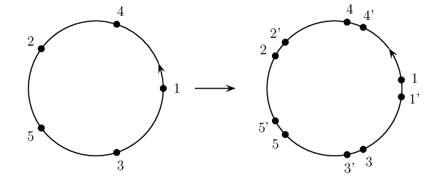
Refer to caption
Figure 2. Convention for splitting labels.

Let surfaced permutations (S1,j1),(S2,j2)∈𝒮​𝒮n(S_{1},j_{1}),(S_{2},j_{2})\in\mathcal{SS}_{n} be given. On the boundary of S2S_{2} there are marked points labeled by numbers 1,…,n1,\dots,n; let us split every marked point kk into a consecutive pair of points kk and k′k^{\prime}, as it is presented on the example from Figure 2. In the second step, for each k∈{1,…,n}k\in\{1,\dots,n\} we glue a small neighborhood of the vertex k∈∂S1k\in\partial S_{1} to a small neighborhood of the vertex k′∈∂S2k^{\prime}\in\partial S_{2} in such a way that the orientations of S1S_{1} and S2S_{2} coincide. In this way we obtain a new surface SS which has marked points on its boundary ∂S\partial S and these are exactly the vertices from ∂S2\partial S_{2} labeled 1,…,n1,\dots,n; we denote the resulting surfaced permutation by (S,j)(S,j) and we call it a product (S1,j1)​(S2,j2)(S_{1},j_{1})(S_{2},j_{2}) of the original surfaced permutations. This choice of gluing surfaces S1S_{1} and S2S_{2} implies that the support of (S1,j1)​(S2,j2)(S_{1},j_{1})(S_{2},j_{2}) is equal to the product of the support of (S1,j1)(S_{1},j_{1}) and the support of (S2,j2)(S_{2},j_{2}).

It is not difficult to explain now the definition of the product of partitioned permutations (Definition 4.9): we treat partitioned permutations as surfaced permutations and compute their product; if the genus of the resulting surface is zero we can identify it with another partitioned permutation, otherwise we set the product to be zero.

It is not difficult to show that for surfaced permutations the product is associative and the associativity of the product of partitioned permutations is a simple corollary.

References

  • [BS04] Z. D. Bai and J. Silverstein: CLT for linear spectral statistics of large-dimensional sample covariance matrices. Ann. Prob., 32: 533–605, 2004.
  • [Bia97] P. Biane: Some properties of crossings and partitions. Discrete Math., 175(1-3):41–53, 1997.
  • [BMS00] M. Bousquet-Mélou and G. Schaeffer. Enumeration of planar constellations. Adv. in Appl. Math., 24(4):337–368, 2000.
  • [BZ93] É. Brézin, A. Zee, Universality of the correlations between eigenvalues of large random matrices, Nuclear Phys. B 402 (1993), no. 3, 613–627.
  • [Col03] B. Collins: Moments and cumulants of polynomial random variables on unitary groups, the Itzykson-Zuber integral, and free probability. Int. Math. Res. Not., (17):953–982, 2003.
  • [CMŚS] B. Collins, J. Mingo, P. Śniady, and R. Speicher: Second order freeness and fluctuations of random matrices: IV. Asymptotic freeness of Jucys-Murphy elements, in preparation.
  • [CŚ04] B. Collins and P. Śniady: Integration with respect to the Haar measure on unitary, orthogonal and symplectic groups. Comm. Math. Phy., 264, (2006), 773 - 795.
  • [Dia03] P. Diaconis: Patterns in Eigenvalues: The 70th Josiah Willard Gibbs Lecture. Bulletin of the AMS, 40: 155-178, 2003.
  • [FMP78] J. B. French, P. A. Mello, A. Pandey, Statistical properties of many-particle spectra. II. Two-point correlations and fluctuations, Ann. of Physics, 113 (1978), no. 2, 277–293.
  • [GM05] A. Guionnet and M. Maïda: A Fourier view on the RR-transform and related asymptotics of spherical integrals. J. Funct. Anal., 222(2):435–490, 2005.
  • [Joh98] K. Johansson: On fluctuations of eigenvalues of random Hermitian matrices. Duke Math. J., 91(1):151–204, 1998.
  • [Jon99] V. F. R. Jones: Planar algebras. I. math.QA/9909027, 1999, 122 pp.
  • [KKP95] A. Khorunzhy, B. Khoruzhenko, L. Pastur, On the 1/N1/N corrections to the Green functions of random matrices with independent entries, J. Phys. A 28 (1995), L31–L35.
  • [Kre72] G. Kreweras: Sur les partitions non croisées d’un cycle. Discrete Math., 1(4):333–350, 1972.
  • [LS59] V. P. Leonov and A. N. Shiryaev: On a method of semi-invariants. Theory of Probability and its Applications, 4, 319–329, 1959.
  • [MN04] J. Mingo and A. Nica: Annular noncrossing permutations and partitions, and second-order asymptotics for random matrices. Int. Math. Res. Not., (28):1413–1460, 2004.
  • [MŚS04] J. Mingo, P. Śniady, and R. Speicher. Second order freeness and fluctuations of random matrices: II. Unitary random matrices. To appear in Adv. in Math..
  • [MS04] J. Mingo and R. Speicher: Second Order Freeness and Fluctuations of Random Matrices: I. Gaussian and Wishart matrices and Cyclic Fock spaces. J. Funct. Anal., 235, 2006, pp. 226-270.
  • [NSp97] A. Nica and R. Speicher: A “Fourier transform” for multiplicative functions on non-crossing partitions. J. Algebraic Combin., 6(2):141–160, 1997.
  • [NSp06] A. Nica and R. Speicher: Lectures on the Combinatorics of Free Probability, London Mathematical Society Lecture Note Series, New York : Cambridge University Press, to appear.
  • [OZ84] K. H. O’Brien and J.-B. Zuber. A note on U⁡(N){\rm U}(N) integrals in the large NN limit. Phys. Lett. B, 144(5-6):407–408, 1984.
  • [Oko00] A. Okounkov: Random matrices and random permutations. Int. Math. Res. Not., 2000, no. 20: 1043–1095, 2000.
  • [Rad04] F. Radulescu: Combinatorial aspectes of Connes’s embedding conjecture and asymptotic distribution of traces of products of unitaries. Preprint, 2004. math.0A/0404308.
  • [Rot64] G.-C. Rota, On the foundations of combinatorial theory. I. Theory of Möbius functions, Z. Wahrscheinlichkeitstheorie und Verw. Gebiete, 2, (1964), 340–368.
  • [Śni05] P. Śniady. Gaussian fluctuations of characters of symmetric groups and of Young diagrams. Preprint arXiv:math.CO/0501112, 2005.
  • [Spe94] R. Speicher: Multiplicative functions on the lattice of noncrossing partitions and free convolution. Math. Ann., 298(4):611–628, 1994.
  • [VDN92] D. V. Voiculescu, K. J. Dykema, and A. Nica. Free random variables. American Mathematical Society, Providence, RI, 1992.
  • [Voi85] D. Voiculescu: Summetries of some reduced free product C∗C^{*}-algebras. In Operator Algebras and their Connections with Topology and Ergodic Theory (Lecture Notes in Mathematics, vol. 1132, Springer-Verlag): 556-588, 1985.
  • [Voi86] D. Voiculescu: Addition of certain non-commuting random variables. J. Funct. Anal., 66: 323–346, 1986.
  • [Voi91] D. Voiculescu: Limit laws for random matrices and free products. Invent. Math., 104(1):201–220, 1991.
  • [Wei78] D. Weingarten: Asymptotic behavior of group integrals in the limit of infinite rank. J. Mathematical Phys., 19(5):999–1001, 1978.
  • [ZJ99] P. Zinn-Justin. Adding and multiplying random matrices: a generalization of Voiculescu’s formulas. Phys. Rev. E (3), 59(5, part A):4884–4888, 1999.