跳到论文正文
W Papers独立论文阅读器 arXiv:math/0606338 论文正文 计算阅读时间 · 0%
引用这篇论文根据当前论文元数据生成,正式投稿前建议核对。


License: Assumed arXiv.org perpetual non-exclusive license
arXiv:math/0606338v1 [math.PR] 14 Jun 2006

Globally centered discrete snakes

Jean-François Marckert
CNRS, LaBRI

Université Bordeaux 1

351 cours de la Libération

33405 Talence cedex, FRANCE

Subject classification : 60J80, 60F17, 60J65.
Keywords: Galton-Watson trees, discrete snake, Brownian snake, Limit theorem.

Abstract

We consider branching random walks built on Galton-Watson trees with offspring distribution having a bounded support, conditioned to have nn nodes, and their rescaled convergences to the Brownian snake. We exhibit a notion of “globally centered discrete snake” that extends the usual settings in which the displacements are supposed centered. We show that under some additional moment conditions, when nn goes to +∞+\infty, “globally centered discrete snakes” converge to the Brownian snake. The proof relies on a precise study of the “lineage” of the nodes in a Galton-Watson tree conditioned by the size, and their links with a multinomial process. Some consequences concerning Galton-Watson trees conditioned by the size are also derived.

1 Introduction

1.1 A model of centered discrete snake

We first begin with the formal description of the notion of trees and branching random walks.

Let T∞={∅}∪⋃n≥1ℕ⋆nT_{\infty}=\{\varnothing\}\cup\bigcup_{n\geq 1}\mathbb{N}^{\star}{}^{n} be the set of finite words on the alphabet ℕ⋆={1,2,…}\mathbb{N}^{\star}=\{1,2,\dots\}. For u=u1​…​unu=u_{1}\ldots u_{n}, and v=v1​…​vm∈T∞v=v_{1}\ldots v_{m}\in T_{\infty}, we let u​v=u1​…​un​v1​…​vmuv=u_{1}\ldots u_{n}v_{1}\ldots v_{m} be the concatenation of the words uu and vv (by convention ∅​u=u​∅=u\varnothing u=u\varnothing=u). Following Neveu, we call planar tree TT a subset of T∞T_{\infty} containing the root ∅\varnothing, and such that if u​i∈Tui\in T, then u∈Tu\in T and for all j∈⟦1,i⟧j\in\llbracket 1,i\rrbracket, u​j∈Tuj\in T. The elements of a tree are called nodes or vertices. For i≠ji\neq j, the nodes u​iui and u​juj are called brothers and uu their father. We let cu​(T)=max⁡{i:u​i∈T}c_{u}(T)=\max\{i:ui\in T\} be the number of children of uu. A node without any child is called a leaf, and we denote by ∂T\partial T the set of leaves of TT. If v≠∅v\not=\varnothing, we say that u​vuv is a descendant of uu and uu is an ancestor of u​vuv. An edge is a pair {u,v}\{u,v\} where uu is the father of vv. A path ⟦u,v⟧\llbracket u,v\rrbracket between the nodes uu and vv in a tree TT is the (minimal) sequence of nodes u:=u0,…,uj:=vu:=u_{0},\dots,u_{j}:=v such that for any i∈⟦0,j−1⟧i\in\llbracket 0,j-1\rrbracket, {ui,ui+1}\{u_{i},u_{i+1}\} is an edge. Set also ⟧u,v⟦=⟦u,v⟧∖{u,v}\rrbracket u,v\llbracket=\llbracket u,v\rrbracket\setminus\{u,v\} and similar notation for ⟦u,v⟦\llbracket u,v\llbracket and for ⟧u,v⟧\rrbracket u,v\rrbracket. The distance dTd_{T}, or simply dd, is the usual graph distance. The depth of uu is |u|=d⁡(∅,u)|u|=d(\varnothing,u). The cardinality of TT is denoted by |T||T|, and we let 𝒯{\mathcal{T}} (resp. 𝒯n{\mathcal{T}}_{n}) be the set of planar trees (resp. with nn edges, i.e. n+1n+1 vertices).

A branching walk is a pair (T,ℓ)(T,\ell) where TT is a tree called the underlying tree and ℓ\ell, the label function, is an application from TT taking its values in ℝ\mathbb{R}. In other words it is a tree in which every vertex owns a real label. We let ℬ{\cal B} be the set of branching walks, and ℬn{\cal B}_{n} be the branching walks associated with trees from 𝒯n{\mathcal{T}}_{n}.

We introduce now some randomness and construct a probability distribution on ℬ{\cal B} and on ℬn{\cal B}_{n}. The set of underlying trees is endowed with the distribution of the family tree of a Galton-Watson (GW) process with offspring distribution μ=(μk)k≥0{\bf\mu}=(\mu_{k})_{k\geq 0} starting from one individual. We denote by 𝐓{\bf T} a random tree under this distribution. The distribution of the labels is defined as follows. Consider (νk)k∈{1,2,…}(\nu_{k})_{k\in\{1,2,\dots\}} a family of distributions, where νk\nu_{k} is a distribution on ℝk\mathbb{R}^{k}. The labels are defined conditionally on the underlying tree 𝐓{\bf T} : Set ℓ⁡(∅)=0\ell(\varnothing)=0, and for any u∈𝐓∖∂𝐓u\in{\bf T}\setminus\partial{\bf T}, consider

Xu:=(ℓ⁡(u​1)−ℓ⁡(u),…,ℓ⁡(u​cu​(𝐓))−ℓ⁡(u)),X_{u}:=\big(\ell(u1)-\ell(u),\dots,\ell(uc_{u}({\bf T}))-\ell(u)\big),

the evolution-vector of the labels between uu and its children. Conditionally on 𝐓{\bf T}, we assume that the r.v. XuX_{u} are independent, and that XuX_{u} has distribution νcu​(𝐓)\nu_{c_{u}({\bf T})}. This determines a distribution on ℬ{\cal B}, denoted by ℙ\mathbb{P}. For example, if νk\nu_{k} is the uniform distribution on {−1,+1}k\{-1,+1\}^{k} for any k>0k>0, then the r.v. ℓ⁡(u​1)−ℓ⁡(u),…,ℓ⁡(u​cu​(𝐓))−ℓ⁡(u)\ell(u1)-\ell(u),\dots,\ell(uc_{u}({\bf T}))-\ell(u) are independent with common distribution 12​(δ+1+δ−1)\frac{1}{2}(\delta_{+1}+\delta_{-1}) (δx\delta_{x} stands for the Dirac mass at xx). In the case where νk\nu_{k} is the uniform distribution on {(1,…,k),(−1,…,−k)}\{(1,\dots,k),(-1,\dots,-k)\}, the r.v. ℓ⁡(u​i)−ℓ⁡(u)\ell(ui)-\ell(u) and ℓ⁡(u​j)−ℓ⁡(u)\ell(uj)-\ell(u) are not independent and do not have the same distribution.

We define now two sets of assumptions (H1)({\rm H}_{1}) and (H2)({\rm H}_{2}) that will be assumed to be satisfied in most of our results. (H1)({\rm H}_{1}) is the conditions that μ\mu is non-degenerate critical and has a bounded support :

(H1):=(μ0+μ1≠1,∑k≥0kμk=1,there exists K>0 s.t. ∑k≤Kμk=1).({\rm H}_{1}):=\Big(\mu_{0}+\mu_{1}\neq 1,\sum_{k\geq 0}k\mu_{k}=1,\textrm{there exists }K>0\textrm{ s.t. }\sum_{k\leq K}\mu_{k}=1\Big).

Under (H1)({\rm H}_{1}) the variance σμ2\sigma^{2}_{\mu} of μ\mu is finite and non zero. The bounded support condition is quite a strong restriction but considering non-bounded distribution leads to non-trivial complications, and we were unable to extend to that case the most important results.

Let Y(k)=(Yk,1,…,Yk,k)Y^{(k)}=(Y_{k,1},\dots,Y_{k,k}) be νk\nu_{k}-distributed, and let mk,jm_{k,j} and σk,j2\sigma_{k,j}^{2} be the mean and the variance of Yk,jY_{k,j}. We call global mean and global variance of the branching random walk,

𝐦=∑k≥1∑j=1kμk​mk,j, and ​β2=∑k≥1∑j=1kμk​𝔼​(Yk,j2).{\bf m}=\sum_{k\geq 1}\sum_{j=1}^{k}\mu_{k}m_{k,j},~~\textrm{ and }~~{\bf\beta}^{2}=\sum_{k\geq 1}\sum_{j=1}^{k}\mu_{k}\mathbb{E}(Y_{k,j}^{2}).

Let (H2)({\rm H}_{2}) denote the conditions that the global mean is null, the global variance finite, and for a p>4p>4, the centered ppth moment of the Yk,jY_{k,j}’s are finite:

(H2):=(𝐦=0​ and ​β∈(0,+∞),there exist p>4 s.t. for any (k,j),1≤j≤k≤K,𝔼(|Yk,j−mk,j|p)<+∞.).({\rm H}_{2}):=\left(\begin{array}[]{l}{\bf m}=0\text{ and }\beta\in(0,+\infty),\\ \hbox{there exist }p>4\hbox{ s.t. for any }(k,j),1\leq j\leq k\leq K,\mathbb{E}\left(|Y_{k,j}-m_{k,j}|^{p}\right)<+\infty.\end{array}\right).

Refer to caption


Figure 1: A tree on which is indicated the depth first traversal, its height and contour process.

Encoding of branching random walks

We study the asymptotic behavior of branching random walks via their encoding by depth first traversal. The depth-first traversal of a tree T∈𝒯nT\in{\cal T}_{n} is a function:

FT:{0,…,2​n}→{ vertices of ​T},F_{T}:\{0,...,2n\}\rightarrow\{\textrm{ vertices of }T\ \},

which we regard as a walk around TT, as follows: FT​(0)=∅{F}_{T}(0)=\varnothing, and given FT​(i)=z{F}_{T}(i)=z, choose if possible and according to the LO, the smallest child ww of zz which has not already been visited, and set FT​(i+1)=wF_{T}(i+1)=w. If not possible, let FT​(i+1)F_{T}(i+1) be the father of zz.

We also denote by ≼\preccurlyeq the lexicographical order (LO) on the planar trees (and u≺vu\prec v if u≼vu\preccurlyeq v and u≠vu\neq v), and let u⁡(k)u(k) be the kk-th vertex in the LO (u⁡(0)=∅u(0)=\varnothing).

We now encode the branching random walk with the help of a pair of processes. For any k∈⟦0,|T−1|⟧k\in\llbracket 0,|T-1|\rrbracket, let HkT=|u⁡(k)|H^{T}_{k}=|u(k)| and RkT=ℓ⁡(u⁡(k))R^{T}_{k}=\ell(u(k)). The height process (HsT,s∈[0,|T−1|])(H^{T}_{s},s\in[0,|T-1|]) and head label process (RsT,s∈[0,|T−1|])(R^{T}_{s},s\in[0,|T-1|]) are obtained from the sequences (HkT)(H^{T}_{k}) and (RkT)(R^{T}_{k}) by linear interpolation. Alternatively, one may encode the branching random walk with a pair of processes associated with the depth first traversal: for any k∈⟦0,2|T|−1⟧k\in\llbracket 0,2|T|-1\rrbracket, let H^T​(k)=|FT​(k)|\widehat{H}^{T}(k)=|F_{T}(k)| and R^kT=ℓ⁡(FT​(k))\widehat{R}^{T}_{k}=\ell(F_{T}(k)). The processes (H^sT,s∈[0,2​|T|−1])(\widehat{H}^{T}_{s},s\in[0,2|T|-1]) and (R^sT,s∈[0,2​|T|−1])(\widehat{R}^{T}_{s},s\in[0,2|T|-1]), obtained by interpolation, are called respectively the contour process and the contour label process; the pair (H^T,R^T)(\widehat{H}^{T},\widehat{R}^{T}) is called the head of the discrete snake.
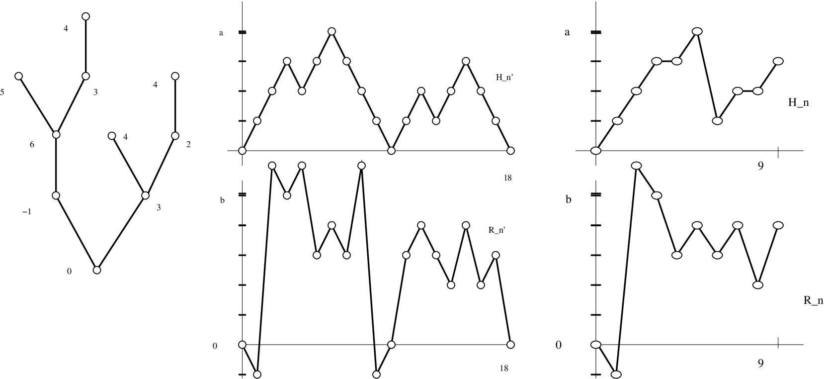
Refer to caption


Figure 2: A branching random walk from ℬ9{\cal B}_{9}. On the first column, the contour process and the contour label process, on the second column, the height process and the height label process.

Let 𝐡n{\bf h}_{n}, 𝐡^n\widehat{\bf h}_{n}, 𝐫n{\bf r}_{n} and 𝐫^n\widehat{{\bf r}}_{n} be the normalized versions of H𝐓H^{{\bf T}}, H^𝐓,R𝐓\widehat{H}^{{\bf T}},R^{{\bf T}}, and R^𝐓\widehat{R}^{{\bf T}} when 𝐓{\bf T} is ℙn\mathbb{P}_{n}-distributed :

𝐡n​(s)=Hn​s𝐓n1/2,𝐡^n​(s)=H^2​n​s𝐓n1/2,𝐫n​(s)=Rn​s𝐓n1/4,𝐫^n​(s)=R^2​n​s𝐓n1/4, for any ​s∈[0,1].{\bf h}_{n}(s)=\frac{H_{ns}^{\bf T}}{n^{1/2}},~~~\widehat{\bf h}_{n}(s)=\frac{\widehat{H}_{2ns}^{\bf T}}{n^{1/2}},~~~{\bf r}_{n}(s)=\frac{R_{ns}^{\bf T}}{n^{1/4}},~~~\widehat{\bf r}_{n}(s)=\frac{\widehat{R}_{2ns}^{\bf T}}{n^{1/4}},\textrm{ for any }s\in[0,1].

Let d:=gcd⁡{k,k≥1,μk>0}d:=\gcd\{k,k\geq 1,\mu_{k}>0\}. The support of the distribution of |𝐓||{\bf T}| – we write supp⁡(|𝐓|)\supp(|{\bf T}|) – is included in 1+d​ℕ1+d\,\mathbb{N} (and ℙ⁡(|𝐓|=1+k​d)>0\mathbb{P}(|{\bf T}|=1+kd)>0 for every kk large enough). For n+1∈supp⁡(|𝐓|)n+1\in\supp(|{\bf T}|), the distribution ℙ\mathbb{P} under the conditioning by |𝐓|=n+1|{\bf T}|=n+1 is denoted by ℙn\mathbb{P}_{n}, in other words ℙn=ℙ(.||𝐓|=n+1)\mathbb{P}_{n}=\mathbb{P}(~.~|\,|{\bf T}|=n+1). Even if not recalled, each statement concerning weak convergence under ℙn\mathbb{P}_{n} is assumed to be along the subsequence (nk)k(n_{k})_{k} for which ℙnk\mathbb{P}_{n_{k}} is well defined. In the proofs, we will treat only the case d=1d=1, the general case being treated with slight modifications.

Theorem 1

If (H1)({\rm H}_{1}) and (H2)({\rm H}_{2}) are satisfied then

(𝐡n,𝐡^n,𝐫n,𝐫^n)→𝑛(d)(𝐡,𝐡,β​𝐫,β​𝐫)\left({\bf h}_{n},\widehat{\bf h}_{n},{\bf r}_{n},\widehat{\bf r}_{n}\right)\xrightarrow[n]{(d)}\left({\bf h},{\bf h},\beta{{\bf r}},\beta{{\bf r}}\right)

in C⁡([0,1],ℝ4)C([0,1],\mathbb{R}^{4}) endowed with the topology of uniform convergence, where 𝐡=2​𝖾/σμ{\bf h}=2{\sf e}/\sigma_{\mu} and 𝖾{\sf e} is the normalized Brownian excursion, and where conditionally on 𝐡{\bf h}, 𝐫{\bf r} is a centered Gaussian process with covariance function

cov⁡(𝐫⁡(s),𝐫⁡(t))=𝐡ˇ​(s,t):=minu∈[s∧t,s∨t]⁡𝐡⁡(u), for any ​s,t∈[0,1].\cov({\bf r}(s),{\bf r}(t))=\check{\bf h}(s,t):=\min_{u\in[s\wedge t,s\vee t]}{\bf h}(u),\textrm{ for any }s,t\in[0,1].

Notice that the same processes 𝐡{\bf h} and 𝐫{\bf r} appear twice in the limit process. The convergence of processes associated with the contour processes (with a ^\widehat{~} ) to the same limit as the one associated with the height processes is well understood now, and “almost” generic (Duquesne & Le Gall [9, Section 2.5] and [20]). In Section 2.7, we prove that we may concentrate only of the height process, as done in this paper. The process (𝐫,𝐡)({\bf r},{\bf h}) (or with a different scaling) is called in the literature head of the Brownian snake with lifetime process the normalized Brownian excursion (BSBE). We refer to the works of Le Gall (e.g. [16] and with Duquesne [10]) for information on the Brownian snake.

In this paper, we deal only with the head of the snake, and not precisely in term of snakes, even if, thanks to the homeomorphism theorem [20], evoked below, Theorem 1 has some applications in term of snakes. We refer to [20, 13] for the notion of discrete snake which is the discrete analogue of BSBE : the discrete snake associated with the branching random walk (T,ℓ)(T,\ell), is the pair (H^T,Φ)(\widehat{H}^{T},\Phi) where Φ=(Φk)k∈⟦0,2|T−1|⟧\Phi=(\Phi_{k})_{k\in\llbracket 0,2|T-1|\rrbracket} and Φk\Phi_{k} is the sequence of labels on the branch ⟦∅,FT(k)⟧\llbracket\varnothing,F_{T}(k)\rrbracket. The title of the present paper is then taken from our model of snake under (H2)({\rm H_{2}}) in which the global mean is 0.

Related works

The convergence 𝐡^n→𝑛(d)𝐡\widehat{\bf h}_{n}\xrightarrow[n]{(d)}{\bf h} is due to Aldous [1, 2] (see also Marckert & Mokkadem [21] for a revisited proof, Pitman [24, Chap. 5 and 6], and Duquesne [9] and Duquesne & Le Gall [10, section 2.5] for generalization to GW trees with offspring distribution having infinite variance).

The two first results concerning the convergence of discrete snakes to the BSBE appeared in two independent works :
∙\bullet Chassaing & Schaeffer [7] deal with discrete snakes built on underlying trees chosen uniformly in 𝒯n{\cal T}_{n} (this corresponds to the case where μ∼G​e​o​m​(1/2)\mu\sim Geom(1/2)) and where the displacements are i.i.d., and for any k,jk,j, νk,j\nu_{k,j} is the uniform distribution in {−1,0,+1}\{-1,0,+1\}. They show the convergence of the head of the snake for the Skohorod topology, and the convergence of the moments of the maximum of 𝐫𝐧\bf r_{n} are also given. This study was motivated by the deep relation between this model of discrete snake and random rooted quadrangulations, underlined by the authors.
∙\bullet Marckert & Mokkadem [20] studied also the case μ∼G​e​o​m​(1/2)\mu\sim Geom(1/2) but with more general centered displacements that have moments of order 6+ε6+\varepsilon (the distribution νk,j\nu_{k,j} does not depend on k,jk,j, but νk\nu_{k} is not assumed to be νk,1×⋯×νk,k\nu_{k,1}\times\dots\times\nu_{k,k}). The convergence of the head of the snake holds in (C⁡[0,1],ℝ2)(C[0,1],\mathbb{R}^{2}) and the convergence of the snake itself is given thanks to a “homeomorphism theorem” which implies that the convergence of the snake and of its tour (in space of continuous functions) are equivalent. Here it implies that under the hypothesis of Theorem 1, the discrete snake associated with our model of labeled trees converges weakly to the BSBE (see [20] for more details).

Then some generalizations appears few months later:
∙\bullet Gittenberger [11] provides a generalization of a lemma from [20] and consider snakes with underlying trees GW trees conditioned by the size (condition equivalent to H1{\rm H}_{1}). The displacements must be centered and have moments of order 8+ε8+\varepsilon.
∙\bullet Janson & Marckert [13] show that in the i.i.d. case (νk,j\nu_{k,j} do not depend on (k,j)(k,j)), moments of order 4+ε4+\varepsilon are necessary and needed to get the convergence the BSBE. If no such moment exists the convergence to a “hairy snake” is proved under the Hausdorff topology.
∙\bullet In Marckert & Miermont [19], the case of νk,j\nu_{k,j} depending of k,jk,j is investigated (also the underlying GW trees are allowed to have two types). The hypothesis are for each k,jk,j, mk,j=0m_{k,j}=0, condition (H2)({\rm H}_{2}) is satisfied, and then ∑k,jμk​σk,j2<+∞\sum_{k,j}\mu_{k}\sigma_{k,j}^{2}<+\infty. A motivation was to generalize the works of Chassaing & Schaeffer [7] concerning quadrangulations to bipartite maps.

Another important point is the convergence of the occupation measure of the head of the discrete snake to the one of the BSBE, the random measure named ISE (the integrated superBrownian excursion introduced by Aldous [3], see also Le Gall [16] and [20, 13]). Using the convergence of discrete snake to the BSBE, Bousquet-Mélou [4] and Bousquet-Mélou & Janson [5] deduce new results on ISE and on the BSBE; for example, some properties on the support of ISE, and of the random density of ISE are derived. We refer also to Le Gall [15] for the convergence of discrete snake conditioned to stay positive.

The novelty in the present paper is that the condition {mk,j=0,∀k,j}\{m_{k,j}=0,\forall k,j\} is replaced by 𝐦=∑k≥1∑j=1kμk​mk,j=0{\bf m}=\sum_{k\geq 1}\sum_{j=1}^{k}\mu_{k}m_{k,j}=0. This allows to consider some natural models where, for example, the displacements are not random knowing the underlying tree (see Section 1.3). The proof of Theorem 1 relies in part on some results from [19], and on a new approach, necessary to control the contribution of the mean of the displacements; the main point for this, is the comparison of the lineage of each node, with some multinomial r.v.  : this is the aim of Theorem 2, that we think interesting in itself, since it reveals a thin global behavior of GW trees conditioned by the size. Unfortunately, the price of this generalization is to consider only offspring distribution with bounded support. The reason comes from the proof of Theorem 2. We guess that some generalization for all families of GW trees (with finite variance) may be found, but for this, a control of an infinite sequence of processes arising in Theorem 2 should be provided, what we were unable to do.

1.2 On the lineage of nodes

Assume that (H1)({\rm H}_{1}) and (H2)({\rm H}_{2}) holds. Let KK be a bound of the offspring distribution. For u=i1​…​ih∈𝐓u=i_{1}\ldots i_{h}\in{\bf T}, let uj=i1​…​iju_{j}=i_{1}\ldots i_{j} and ⟦∅,u⟧={∅=u0,u1,…,u|u|}\llbracket\varnothing,u\rrbracket=\{\varnothing=u_{0},u_{1},\ldots,u_{|u|}\} be the ancestral line of uu back to the root. Conditionally on 𝐓{\bf T}, l⁡(u)l(u) owns the following representations :

ℓ⁡(u)=∑m=1|u|ℓ⁡(um)−ℓ⁡(um−1).\ell(u)=\sum_{m=1}^{|u|}\ell(u_{m})-\ell(u_{m-1}). (1)

where l⁡(um)−l⁡(um−1)l(u_{m})-l(u_{m-1}) is νk,j\nu_{k,j}-distributed when cum−1​(T)=kc_{u_{m-1}}(T)=k and im=ji_{m}=j, where νk,j\nu_{k,j} is the jjth marginal of νk\nu_{k}, and where the r.v. (ℓ⁡(um)−ℓ⁡(um−1))(\ell(u_{m})-\ell(u_{m-1}))’s are independent; the variables ℓ⁡(um)−ℓ⁡(um−1)\ell(u_{m})-\ell(u_{m-1}) will be often called displacements.

Consider the array IK={(k,j),1≤j≤k≤K}I_{K}=\left\{(k,j),1\leq j\leq k\leq K\right\}. Let uu be a node of TT. For any (k,j)∈IK(k,j)\in I_{K}, let Au,k,j​(T)A_{u,k,j}(T) be the number of strict ancestors vv of uu (the nodes v∈⟦∅,u⟦v\in\llbracket\varnothing,u\llbracket) such that cv​(T)=kc_{v}({T})=k, and such that uu is a descendant of v​jvj, the jjth child of vv (we write fv​(u)=jf_{v}(u)=j). We say that vv is an ancestor of type k,jk,j of uu, and we call the vector Au=(Au,i)i∈IKA_{u}=(A_{u,i})_{i\in I_{K}} the lineage of uu (or the content of ⟦∅,u⟧\llbracket\varnothing,u\rrbracket). See Figure 3.

Refer to caption


Figure 3: On this tree Au,1,1=1,Au,2,2=1,Au,4,2=1,Au,5,3=1A_{u,1,1}=1,A_{u,2,2}=1,A_{u,4,2}=1,A_{u,5,3}=1, the others Au,iA_{u,i} are 0.

By (1), conditionally on 𝐓{\bf T}, the label ℓ⁡(u)\ell(u) owns the following representations :

ℓ⁡(u)=(d)∑(k,j)∈IK∑l=1Au,k,jYk,j(l),\ell(u)\mathrel{\mathop{\kern 0.0pt=}\limits^{(d)}}\sum_{(k,j)\in I_{K}}\sum_{l=1}^{A_{u,k,j}}Y_{k,j}^{(l)},

where the r.v. Yk,j(l)Y_{k,j}^{(l)} are independent, and where for any ll, Yk,jY_{k,j} is νk,j\nu_{k,j} distributed. In order to make more apparent the contribution of the mk,jm_{k,j}’s , and using that 𝐦=0{\bf m}=0, write

ℓ⁡(u)=(d)∑(k,j)∈IK∑l=1Au,k,j(Yk,j(l)−mk,j)+∑(k,j)∈IK(Au,k,j−μk​|u|)​mk,j.\ell(u)\mathrel{\mathop{\kern 0.0pt=}\limits^{(d)}}\sum_{(k,j)\in I_{K}}\sum_{l=1}^{A_{u,k,j}}\big(Y_{k,j}^{(l)}-m_{k,j}\big)+\sum_{(k,j)\in I_{K}}\left(A_{u,k,j}-\mu_{k}|u|\right)m_{k,j}. (2)

Assume that 𝐓{\bf T} is ℙn\mathbb{P}_{n} distributed, and that u=u⁡(n​s)u=u(ns) for some s∈(0,1)s\in(0,1). Conditionally on |u||u|, we will see that both parts of the right hand side of (2) divided by n1/4n^{1/4} converge in distribution, and the limit r.v. are independent : in the first part, the fluctuations of Au,k,jA_{u,k,j} around μk​|u|\mu_{k}|u| are not important, while in the second sum only the fluctuations of Au,k,jA_{u,k,j} around μk​|u|\mu_{k}|u| matter.

We now concentrate on the r.v. (Au)′​s(A_{u})^{\prime}s under ℙn\mathbb{P}_{n}. For any l∈⟦0,n⟧l\in\llbracket 0,n\rrbracket, (k,j)∈IK(k,j)\in I_{K}, set

𝐠(k,j)(n)​(l):=Au⁡(l),k,j−μk​|u⁡(l)|.{\bf g}^{(n)}_{(k,j)}(l):=A_{u(l),k,j}-\mu_{k}|u(l)|.

For every (k,j)∈IK{(k,j)\in I_{K}}, the process l→𝐠(k,j)(n)​(l)l\to{\bf g}^{(n)}_{(k,j)}(l) encodes the evolution of the number of ancestors of type k,jk,j of u⁡(l)u(l), when ll varies. Consider 𝐆(n)=(𝐆(n)​(s))s∈[0,1]{\bf G}^{(n)}=({\bf G}^{(n)}(s))_{s\in[0,1]} the process taking its values in ℝIK\mathbb{R}^{I_{K}} defined by : For any ss, 𝐆(n)​(s)=(𝐆k,j(n)​(s))(k,j)∈IK{\bf G}^{(n)}(s)=\big({\bf G}^{(n)}_{k,j}(s)\big)_{(k,j)\in I_{K}} where s→𝐆k,j(n)​(s)s\to{\bf G}^{(n)}_{k,j}(s) is the real continuous process that interpolates 𝐠k,j(n){\bf g}^{(n)}_{k,j} as follows :

𝐆k,j(n)​(s):=𝐠k,j(n)​(⌊n​s⌋)+{n​s}​(𝐠k,j(n)​(⌊n​s+1⌋)−𝐠k,j(n)​(⌊n​s⌋))n1/4,s∈[0,1].{\bf G}^{(n)}_{k,j}(s):=\frac{{\bf g}^{(n)}_{k,j}(\lfloor ns\rfloor)+\{ns\}\big({\bf g}^{(n)}_{k,j}(\lfloor ns+1\rfloor)-{\bf g}^{(n)}_{k,j}(\lfloor ns\rfloor)\big)}{n^{1/4}},~~~s\in[0,1]. (3)

The random process 𝐆(n){\bf G}^{(n)} encodes the lineage of all the nodes of 𝐓{\bf T}, and its limiting behavior is described by the following theorem.

Theorem 2

Under (H1)({\rm H}_{1}), (H2)({\rm H}_{2}) the following convergence in distribution holds in C​([0,1])#​IK×C⁡[0,1]C([0,1])^{\#I_{K}}\times C[0,1] endowed with the topology of the uniform convergence

(𝐆(n),𝐡n)→𝑛(d)(𝐆,𝐡)({\bf G}^{(n)},{\bf h}_{n})\xrightarrow[n]{(d)}({\bf G},{\bf h})

where 𝐡{\bf h} is defined as in Theorem 1 and 𝐆=(𝐆k,j​(s))(k,j)∈IK,s∈[0,1]{\bf G}=({\bf G}_{k,j}(s))_{(k,j)\in I_{K},s\in[0,1]} is a real centered Gaussian field with the following covariance function : for any (k,j)(k,j) and (k′,j′)(k^{\prime},j^{\prime}) in IKI_{K}, ss and s′s^{\prime} in [0,1][0,1],

cov⁡(𝐆k,j​(s),𝐆k′,j′​(s′))=(−μk​μk′+μk​1(k,j)=(k′,j′))​𝐡ˇ​(s,s′).\cov\big({\bf G}_{k,j}(s),{\bf G}_{k^{\prime},j^{\prime}}(s^{\prime})\big)=\left(-\mu_{k}\mu_{k^{\prime}}+\mu_{k}\textrm{\dsrom{1}}_{(k,j)=(k^{\prime},j^{\prime})}\right)\check{{\bf h}}(s,s^{\prime}). (4)

1.3 Comments, examples and applications

1) Theorem 2 may be considered as the strongest result of this paper. It gives very precise information on the asymptotic behavior of the process 𝐆n{\bf G}_{n} that encodes the lineage of all the nodes. This gives a “global asymptotic” property reminiscent of the properties of the distinguished branch in “a size biased GW tree” (see [17, chap. 11]). The restriction to offspring distributions having a bounded support comes from the proof of this result.

2) For any fixed (k,j)∈IK(k,j)\in I_{K}, knowing 𝐡{\bf h}, 𝐆k,j{\bf G}_{k,j} is a Gaussian process with covariance function

cov⁡(𝐆k,j​(s),𝐆k,j​(s′))=(−μk2+μk)​𝐡ˇ​(s,s′).\cov\big({\bf G}_{k,j}(s),{\bf G}_{k,j}(s^{\prime})\big)=\left(-\mu_{k}^{2}+\mu_{k}\right)\check{{\bf h}}(s,s^{\prime}).

In other words, the processes (𝐆k,j,𝐡)({\bf G}_{k,j},{\bf h}) has the same distribution as (−μk2+μk​𝐫,𝐡)(\sqrt{-\mu_{k}^{2}+\mu_{k}}\,{\bf r},{\bf h}), and then up to some multiplicative constants, (𝐆k,j,𝐡)({\bf G}_{k,j},{\bf h}) is the head of a BSBE. As a simple consequence of Theorem 2, we have that (𝐆k,j,𝐡)(k,j)∈IK({\bf G}_{k,j},{\bf h})_{(k,j)\in I_{K}} is a sequence of heads of BSBE, and that for any (k,j)∈IK(k,j)\in I_{K},

(𝐆k,j(n),𝐡n)→𝑛(d)(𝐆k,j,𝐡).\big({\bf G}^{(n)}_{k,j},{\bf h}_{n}\big)\xrightarrow[n]{(d)}\big({\bf G}_{k,j},{\bf h}\big). (5)

The dependence between the different processes 𝐆k,j{\bf G}_{k,j} is ruled out by (4). For any families of real numbers (λk,j)(k,j)∈IK(\lambda_{k,j})_{(k,j)\in I_{K}}, we have

(∑(k,j)∈IKλk,j​𝐆k,j(n),𝐡n)→𝑛(d)(∑k,jλk,j​𝐆k,j,𝐡).\left(\sum_{(k,j)\in I_{K}}\lambda_{k,j}{\bf G}^{(n)}_{k,j},{\bf h}_{n}\right)\xrightarrow[n]{(d)}\left(\sum_{k,j}\lambda_{k,j}{\bf G}_{k,j},{\bf h}\right). (6)

We would like to stress on the following point: discrete snake are usually constructed with “two levels of randomness” : the underlying trees are random and so are the displacements given the underlying tree, and then BSBE appears to be a natural limit of these objects . Here, we provide some objects with only “one level of randomness” that converge to the Brownian snake. The BSBE appears as a kind of internal complexity measure in trees measuring the difference between the number of ancestors of type k,jk,j and some expected quantities.

3) Consider the case μ=12​(δ0+δ2)\mu=\frac{1}{2}(\delta_{0}+\delta_{2}), ν2=δ(+1,−1)\nu_{2}=\delta_{(+1,-1)}, of binary trees in which the displacements are not random: ℓ⁡(u​1)−ℓ⁡(u)=+1\ell(u1)-\ell(u)=+1 and ℓ⁡(u​2)−ℓ⁡(u)=−1\ell(u2)-\ell(u)=-1. We have 𝐦=0{\bf m}=0 and β2=12​(1+1)=1\beta^{2}=\frac{1}{2}(1+1)=1 and Theorems 1 and 2 apply. Hence, the clear positive bias for Rn​(t)R_{n}(t) for small values of tt, disappears at the limit. Note also that this normalizing factor is exactly the same as if ν2=12​(δ(+1,−1)+δ(−1,+1))\nu_{2}=\frac{1}{2}(\delta_{(+1,-1)}+\delta_{(-1,+1)}) (case where (ℓ⁡(u​1)−ℓ⁡(u),ℓ⁡(u​2)−ℓ⁡(u))(\ell(u1)-\ell(u),\ell(u2)-\ell(u)) is equally likely (+1,−1)(+1,-1) or (−1,+1)(-1,+1)) and as if ν2=(12​(δ+1+δ−1))2\nu_{2}=(\frac{1}{2}(\delta_{+1}+\delta_{-1}))^{2} (case where the ℓ⁡(u​1)−ℓ⁡(u)\ell(u1)-\ell(u) and ℓ⁡(u​2)−ℓ⁡(u)\ell(u2)-\ell(u) are i.i.d., uniform on {−1,1}\{-1,1\}). The question of the convergence of the discrete snake in the case ν2=δ(+1,−1)\nu_{2}=\delta_{(+1,-1)} appears first in Marckert [18] in relation with some properties of the rotation correspondence, and the difference between left and right depth in binary trees . The convergence of (𝐫n)({\bf r}_{n}) is not given in [18], but the convergence of the occupation measure of 𝐫n{\bf r}_{n}, “the discrete ISE”, to ISE is established. We refer also to Janson [12] for recent developments concerning the same question.

Further, notice that in this model, the label ℓ⁡(u)\ell(u) of a vertex uu is ℓ⁡(u)=Au,2,1−Au,2,2,\ell(u)=A_{u,2,1}-A_{u,2,2}, that is the number of left steps minus the number of right steps necessary to climb from the root to uu in the binary tree. The convergence of (𝐫n)({\bf r}_{n}) can be seen directly via the one of (𝐆(n))({\bf G}^{(n)}).

(𝐆2,1(n),𝐆2,2(n),𝐡n)→𝑛(d)(𝐆2,1,𝐆2,2,𝐡),({\bf G}_{2,1}^{(n)},{\bf G}_{2,2}^{(n)},{\bf h}_{n})\xrightarrow[n]{(d)}\big({\bf G}_{2,1},{\bf G}_{2,2},{\bf h}\big), (7)

and then 𝐫n=𝐆2,1(n)−𝐆2,2(n)→𝑛(d)𝐆2,1−𝐆2,2{\bf r}_{n}={\bf G}_{2,1}^{(n)}-{\bf G}_{2,2}^{(n)}\xrightarrow[n]{(d)}{\bf G}_{2,1}-{\bf G}_{2,2} which is, conditionally to 𝐡{\bf h} and according to (4), a centered Gaussian process with covariance function 𝐡ˇ​(s,t)\check{{\bf h}}(s,t). Here, the convergence of (𝐫n)({\bf r}_{n}) appears to be a consequence of the convergence of 𝐆2,1{\bf G}_{2,1} and 𝐆2,2{\bf G}_{2,2}, encoding the right depth and the left depth in binary trees.

2 Proofs

The proofs rely on a precise study of the lineage of the nodes under ℙn\mathbb{P}_{n} and in particular on the comparison of AuA_{u} with a multinomial random variable. For this reason we first give some elements on multinomial distributions and on their asymptotic behaviors. We then proceed to the proof of Theorem 2, showing first the convergence of the uni-dimensional distribution then the convergence of the finite-dimensional distribution. The proof of Theorem 1 is given afterward. We think that some points of view especially in the description of the distribution of the lineages in trees under ℙn\mathbb{P}_{n} should provide some new approaches to study the trees under ℙn\mathbb{P}_{n}.

2.1 Prerequisite on multinomial distributions

The contents of this section is quite classical. Consider 𝐩=(pi)i∈IK{\bf p}=(p_{i})_{i\in I_{K}} the distribution on IKI_{K}, defined by

pk,j:=μk for any ​(k,j)∈IK.p_{k,j}:=\mu_{k}~~~~\textrm{ for any }(k,j)\in I_{K}.

We say that ℳ(h){\cal M}^{(h)} is a multinomial r.v. with parameter hh and 𝐩{\bf p}, if, for any 𝗆=(𝗆i)i∈IK{\sf m}=({\sf m}_{i})_{i\in I_{K}}

ℚh​({𝗆}):=ℙ⁡(ℳ(h)=𝗆)=(h(𝗆i)i∈IK)​∏i∈IKpi𝗆i​1ℕI​[h]​(𝗆)\mathbb{Q}_{h}(\{{\sf m}\}):=\mathbb{P}({\cal M}^{(h)}={\sf m})=\binom{h}{({\sf m}_{i})_{i\in I_{K}}}\prod_{i\in I_{K}}p_{i}^{{\sf m}_{i}}\,\,\textrm{\dsrom{1}}_{\mathbb{N}^{I}[h]}({\sf m})

where (h(𝗆i)i∈IK)=h!/(∏i∈IK𝗆i!),\binom{h}{({\sf m}_{i})_{i\in I_{K}}}=h!/(\prod_{i\in I_{K}}{\sf m}_{i}!), and where for any n≥1n\geq 1, ℕI​[n]\mathbb{N}^{I}[n] is the set of elements c=(ci)i∈IKc=(c_{i})_{i\in I_{K}} of ℕ#​IK{\mathbb{N}}^{\#I_{K}}, such that ∑i∈IKci=n\sum_{i\in I_{K}}c_{i}=n.

Recall that for any i∈IKi\in I_{K}, ℳi(h){\cal M}_{i}^{(h)} is a binomial r.v. with parameters nn and pip_{i}.

In order to fit with further considerations, we introduce the #​IK\#I_{K} dimensional real vector 𝒢⁡(n,h)=(𝒢i​(n,h))i∈IK{\cal G}({n,h})=({\cal G}_{i}({n,h}))_{i\in I_{K}} defined by

𝒢k,j(n,h)=n−1/4(ℳk,j(h)−μkh) for any (k,j)∈IK.{\cal G}_{k,j}(n,h)=n^{-1/4}\big({\cal M}^{(h)}_{k,j}-\mu_{k}\,h\big)~~~\textrm{ for any }(k,j)\in I_{K}.

Let 𝒢∞=(𝒢∞,i)i∈IK{\cal G}_{\infty}=({\cal G}_{\infty,_{i}})_{i\in I_{K}} be a centered Gaussian vector having as covariance function

cov⁡(𝒢∞,i,𝒢∞,i′)=−pi​pi′+pi​1i=i′ for any ​i,i′∈IK.\cov({\cal G}_{\infty,i},{\cal G}_{\infty,i^{\prime}})=-p_{i}p_{i^{\prime}}+p_{i}\textrm{\dsrom{1}}_{i=i^{\prime}}~~~~\textrm{ for any }i,i^{\prime}\in I_{K}. (8)
Proposition 3

Let (h⁡(n))(h(n)) be a sequence of positive integers s.t. h⁡(n)/n→λ∈(0,+∞)h(n)/\sqrt{n}\to\lambda\in(0,+\infty). Under (H1)({\rm H}_{1}) we have 𝒢⁡(n,h⁡(n))→𝑛(d)λ​𝒢∞{\cal G}({n,h(n)})\xrightarrow[n]{(d)}\sqrt{\lambda}\,{\cal G}_{\infty} in ℝ#​IK\mathbb{R}^{\#I_{K}}.

Proof. This may be proved using classical tools. As pointed out by E. Rio in a personal discussion, this is also a consequence of the convergence of the empirical process to the Brownian bridge. We only sketch the proof (for λ=1\lambda=1) : let (Ul)l(U_{l})_{l} be a sequence of i.i.d. r.v. uniform on [0,1]. Let FnF_{n} be the associated empirical distribution function and FF the distribution function of UU. Denote by gn=Fn−Fg_{n}=F_{n}-F. According to Donsker [8], n​gn→𝑛(d)𝖻\sqrt{n}g_{n}\xrightarrow[n]{(d)}{\sf b} where 𝖻{\sf b} is a normalized Brownian bridge.

Take 𝐪=(ql)l∈ℕ{\bf q}=(q_{l})_{l\in\mathbb{N}} a distribution on ℕ\mathbb{N} and consider 𝒩k(n)=#{j,1≤j≤n,Uj∈[q1+⋯+qk,q1+⋯+qk+1]}{\cal N}_{k}^{(n)}=\#\{j,1\leq j\leq n,U_{j}\in[q_{1}+\dots+q_{k},q_{1}+\dots+q_{k+1}]\}. Then (𝒩k(n))k≥1({\cal N}_{k}^{(n)})_{k\geq 1} is a multinomial r.v. with parameters nn and 𝐪{\bf q} and satisfies

(𝒩k(n)−qk​n)/n=n​(gn​(q1+⋯+qk+1)−gn​(q1+⋯+qk)).({\cal N}_{k}^{(n)}-q_{k}n)/\sqrt{n}=\sqrt{n}\big(g_{n}(q_{1}+\dots+q_{k+1})-g_{n}(q_{1}+\dots+q_{k})\big).

By Donsker, for any L>0L>0, ((𝒩k(n)−qk​n)/n)k≤L\big(({\cal N}_{k}^{(n)}-q_{k}n)/\sqrt{n}\big)_{k\leq L} converges in distribution to (𝖻q1+⋯+qk+1−𝖻q1+⋯+qk)k≤L({\sf b}_{q_{1}+\dots+q_{k+1}}-{\sf b}_{q_{1}+\dots+q_{k}})_{k\leq L}. The properties of 𝖻{\sf b} allow to conclude. □\Box

The following Proposition will be used in the proof of the tightness of (𝐆(n))({\bf G}^{(n)}).

Proposition 4

Under (H1)({\rm H}_{1}), for any β>1\beta>1, there exists c>0c>0 such that, for any h>0h>0, any n>0n>0,

𝔼⁡(‖𝒢⁡(n,h)‖1β)≤c​(h/n)β/2.\mathbb{E}\left(\big\|{\cal G}({n,h})\|_{1}^{\beta}\right)\leq c\left({h}/{\sqrt{n}}\,\right)^{\beta/2}.

Recall that all the norms are equivalent in ℝ#​IK\mathbb{R}^{\#I_{K}}. Here, we use ‖U‖1=∑(k,j)∈IK|Uk,j|\|U\|_{1}=\sum_{(k,j)\in I_{K}}|U_{k,j}|. 
Proof. First, since ‖U‖1β≤c​∑|Uk,j|β\|U\|_{1}^{\beta}\leq c\sum|U_{k,j}|^{\beta} for some c>0c>0, 𝔼(∥𝒢(n,h)∥1β)≤c∑(k,j)∈IK𝔼(|n−1/4(ℳk,j(h)−μkh)|β)\mathbb{E}\left(\big\|{\cal G}({n,h})\|_{1}^{\beta}\right)\leq c\sum_{(k,j)\in I_{K}}\mathbb{E}(|n^{-1/4}\big({\cal M}^{(h)}_{k,j}-\mu_{k}\,h\big)|^{\beta}). Since ℳk,j(h){\cal M}^{(h)}_{k,j} is a binomial random variable with parameter μk\mu_{k} and hh, 𝔼⁡(|(ℳk,j(h)−μk​h)|β)≤C⁡(μk,β)​hβ/2\mathbb{E}(|\big({\cal M}^{(h)}_{k,j}-\mu_{k}\,h\big)|^{\beta})\leq C({\mu_{k},\beta})h^{\beta/2} where the constant C⁡(μk,β)C({\mu_{k},\beta}) depends on μk\mu_{k} and β\beta (see Petrov [23], th. 2.10 p.62).  □\Box

2.2 Decomposition of trees using the lineages

For any k∈ℕk\in\mathbb{N}, a forest with kk roots is a kk-tuple of planar trees f=(t1,…,tk){f}=(t^{1},\ldots,t^{k}). The size |f||f| of f{f} is |t1|+…​|tk||t^{1}|+\ldots|t^{k}|. We denote by 𝐟k=(𝐓1,…,𝐓k){\bf f}_{k}=({\bf T}^{1},\dots,{\bf T}^{k}) a random forest in which the trees 𝐓1,…,𝐓k{\bf T}^{1},\dots,{\bf T}^{k} are i.i.d. GW trees with offspring distribution μ\mu. For any 𝖺=(𝖺k,j)(k,j)∈IK∈ℝI{\sf a}=({\sf a}_{k,j})_{(k,j)\in I_{K}}\in{\mathbb{R}}^{I}, write

N1​(𝖺)=∑(k,j)∈IK(j−1)​𝖺k,j and N2​(𝖺)=∑(k,j)∈IK(k−j)​𝖺k,j.N_{1}({\sf a})=\sum_{(k,j)\in I_{K}}(j-1){\sf a}_{k,j}~~~~\textrm{ and }~~~~N_{2}({\sf a})=\sum_{(k,j)\in I_{K}}(k-j){\sf a}_{k,j}.
Proposition 5

Let hh be a non-negative integer. For any 𝖺∈ℕI​[h]{\sf a}\in{\mathbb{N}}^{I}[h], and any m∈⟦0,n⟧m\in\llbracket 0,n\rrbracket :

ℙn​(Au⁡(m)=𝖺)=ℚh​(𝖺)​ℙ⁡(|𝐟N1​(𝖺)|=m−h,|𝐟1+N2​(𝖺)′|=n+1−m)ℙ⁡(|𝐓|=n),\mathbb{P}_{n}\left(A_{u(m)}={\sf a}\right)=\mathbb{Q}_{h}({\sf a})\frac{\mathbb{P}\left(|{\bf f}_{N_{1}({\sf a})}|=m-h,\,|{\bf f}\,^{\prime}_{1+N_{2}({\sf a})}|=n+1-m\right)}{\mathbb{P}(|{\bf T}|=n)}, (9)

where 𝐟{\bf f} and 𝐟′{\bf f}\,^{\prime} are two independent forests.

Proof. To build a tree TT of 𝒯n{\cal T}_{n} such that Au⁡(m)=𝖺A_{u(m)}={\sf a}, we first build the branch b=⟦∅,u(m)⟧b=\llbracket\varnothing,u(m)\rrbracket : Exactly 𝖺k,j{\sf a}_{k,j} ancestors vv among the hh strict ancestors of uu satisfy (cv​(T),fv​(u))=(k,j)(c_{v}(T),f_{v}(u))=(k,j). Hence, there are (n𝖺)\binom{n}{{\sf a}} way to build bb. Then, we complete bb in grafting on its neighbors some subtrees satisfying the following constraints. When Au⁡(m)=𝖺A_{u(m)}={\sf a}, the number of subtrees rooted on the neighbors of the branch ⟦∅,u(m)⟦\llbracket\varnothing,u(m)\llbracket visited before u⁡(m)u(m) (resp. after u⁡(m)u(m)) are respectively

N1​(𝖺)\displaystyle N_{1}({\sf a}) =\displaystyle= #{w,d(⟦∅,u(m)⟦,w)=1,w≺u(m)},\displaystyle\#\big\{w,d(\llbracket\varnothing,u(m)\llbracket,w)=1,w\prec u(m)\big\},
1+N2​(𝖺)\displaystyle 1+N_{2}({\sf a}) =\displaystyle= #({u(m)}∪{w,d(⟧u(m),∅⟧,w)=1,u(m)≺w}).\displaystyle\#\left(\{u(m)\}\cup\big\{w,d(\rrbracket u(m),\varnothing\rrbracket,w)=1,u(m)\prec w\big\}\right).

See an illustration on Figure 4.

Refer to caption


Figure 4: The two forests considered in the decomposition

The N1​(𝖺)N_{1}({\sf a}) subtrees must contain exactly m−|u⁡(m)|m-|u(m)| nodes (the nodes, among the m+1m+1 first, not on ⟦∅,u(m)⟧\llbracket\varnothing,u(m)\rrbracket), and the 1+N2​(𝖺)1+N_{2}({\sf a}) subtrees must contain exactly n+1−mn+1-m nodes (the nodes visited after u⁡(m)u(m), u⁡(m)u(m) included). In other words, we need two forests containing respectively m−hm-h and n+1−mn+1-m nodes. Hence, using simple considerations on the probability distribution of GW trees we get the announced result.   □\Box

A consequence of this Proposition is

ℙn​(|u​(m)|=h)\displaystyle\mathbb{P}_{n}\left(|u(m)|=h\right) =\displaystyle= ∑𝗑∈ℕI​[h]ℚh​(𝗑)​ℙ⁡(|𝐟N1​(𝗑)|=m−h,|𝐟1+N2​(𝗑)′|=n+1−m)ℙ⁡(|𝐓|=n)\displaystyle\sum_{{\sf x}\in\mathbb{N}^{I}[h]}\mathbb{Q}_{h}({\sf x})\frac{\mathbb{P}(|{\bf f\,}_{N_{1}({\sf x})}|=m-h,|{\bf f\,}^{\prime}_{1+N_{2}({\sf x})}|=n+1-m)}{\mathbb{P}(|{\bf T}|=n)} (10)
=\displaystyle= ℙ⁡(|𝐟N1​(ℳ(h))|=m−h,|𝐟1+N2​(ℳ(h))′|=n+1−m)ℙ⁡(|𝐓|=n).\displaystyle\frac{\mathbb{P}\left(|{\bf f}_{N_{1}({\cal M}^{(h)})}|=m-h,|{\bf f\,}^{\prime}_{1+N_{2}({\cal M}^{(h)})}|=n+1-m\right)}{\mathbb{P}(|{\bf T}|=n)}. (11)

where ℳ(h){\cal M}^{(h)} is a multinomial random variable with parameters hh and 𝐩{\bf p}.

2.2.1 Few fact concerning random forests and random trees

Let (Wi)i≥0(W_{i})_{i\geq 0} be a random walk starting from 0 with i.i.d. increments with distribution (μ~k)k≥−1=(μk+1)k≥−1(\tilde{\mu}_{k})_{k\geq-1}=(\mu_{k+1})_{k\geq-1} (that is with increment ξ−1\xi-1, where ξ\xi is μ\mu-distributed). We have

Lemma 6

Assume (H1)({\rm H}_{1}).
(i) (Otter [22]) For any k≥1k\geq 1 and n≥kn\geq k, ℙ⁡(|𝐟k|=n)=kn​ℙ​(Wn=−k).\displaystyle\mathbb{P}(|\,{\bf f\,}_{k}|=n)=\frac{k}{n}\,\mathbb{P}(W_{n}=-k).
(ii) (Central local limit theorem (CLLT) )

supl∈−n+d​ℕ|nd​ℙ​(Wn=l)−12​π​σμ​exp⁡(−l22​σμ2​n)|→𝑛0.\sup_{l\in-n+d\mathbb{N}}\left|\frac{\sqrt{n}}{d}\,\mathbb{P}(W_{n}=l)-\frac{1}{\sqrt{2\pi}\sigma_{\mu}}\exp\left(-\frac{l^{2}}{2\sigma_{\mu}^{2}n}\right)\right|\xrightarrow[~~n~~]{}0. (12)

(iii) supn≥0supx≥0x​ℙ​(Wn=x)<+∞.\sup_{n\geq 0}\sup_{x\geq 0}~x\,\mathbb{P}(W_{n}=x)\,<+\infty.

(i)(i) is often called “conjugation of tree principle” or “cyclical lemma”, and may be found in Pitman [24, chap 5.1] and is usually attributed to Otter, Kemperman or Dvoretzky-Motzkin.
(i​i)(ii) is usually called the central local limit theorem (see Breuillard [6] for a state of the art). Recall that dd is the span of μ\mu. The support of WnW_{n} is included in −n+d​ℕ={u∈ℤ,u=−n+d​i,i∈ℕ}-n+d\mathbb{N}=\{u\in\mathbb{Z},u=-n+di,i\in\mathbb{N}\}. A consequence of (i)(i) and (i​i)(ii) is that

ℙ⁡(|𝐓|=n)∼dn−3/22​π​σμ,\mathbb{P}(|{\bf T}|=n)\sim\frac{dn^{-3/2}}{\sqrt{2\pi}\sigma_{\mu}}, (13)

the equivalent being taken along the subsequence where the left hand side is non-null.
Proof of (i​i​i)(iii): supn≥0supx≥c​n{x​ℙ​(Wn=x)}\sup_{n\geq 0}\sup_{x\geq c\sqrt{n}}\{x\,\mathbb{P}(W_{n}=x)\} is bounded by the Tchebichev inequality. By (i​i)(ii), supx≤c​nn​ℙ​(Wn=x)⟶nd2​π​σμ\sup_{x\leq c\sqrt{n}}\sqrt{n}\,\mathbb{P}(W_{n}=x)\mathrel{\mathop{\kern 0.0pt\longrightarrow}\limits_{n}}\frac{d}{\sqrt{2\pi}\sigma_{\mu}}, then supn≥0supx≤c​nn​ℙ​(Wn=x)\sup_{n\geq 0}\sup_{x\leq c\sqrt{n}}\sqrt{n}\,\mathbb{P}(W_{n}=x) is finite. □\Box

The following Lemma controls the maximum increment in the process HH under ℙn\mathbb{P}_{n}.

Lemma 7

Assume (H1)({\rm H}_{1}). For any c>0c>0 then exists ρ>0\rho>0 such that

ℙn​(maxl⁡{||u⁡(l+1)|−|u⁡(l)||}≥ρ​log⁡n)=O⁡(n−c).\mathbb{P}_{n}\Big(\max_{l}\left\{\big||u(l+1)|-|u(l)|\big|\right\}\geq\rho\log n\Big)=O(n^{-c}).

Proof. We just sketch the proof that deeply relies on the conjugation of tree principle. Take n+1n+1 i.i.d. r.v. X1,…,Xn+1X_{1},\dots,X_{n+1}, μ\mu-distributed. Conditionally on ∑i=1n+1(Xi−1)=−1\sum_{i=1}^{n+1}(X_{i}-1)=-1, among the n+1n+1 shifted sequences (X1,…,Xn+1)(X_{1},\dots,X_{n+1}), (X2,…,Xn+1,X1),…,(Xn+1,X1,…,Xn)(X_{2},\dots,X_{n+1},X_{1}),\dots,(X_{n+1},X_{1},\dots,X_{n}), exactly one (X1⋆,…,Xn+1⋆)(X_{1}^{\star},\dots,X_{n+1}^{\star}) corresponds to a sequence (cu,u∈T)(c_{u},u\in T) for a tree T∈𝒯nT\in{\cal T}_{n} (where the cuc_{u} are sorted according the depth first order), and (X1⋆,…,Xn+1⋆)=(d)(cu,u∈𝐓)(X_{1}^{\star},\dots,X_{n+1}^{\star})\mathrel{\mathop{\kern 0.0pt=}\limits^{(d)}}(c_{u},u\in{\bf T}) for 𝐓{\bf T} under ℙn\mathbb{P}_{n}.

The inequality ||u⁡(l)|−|u⁡(l+1)||=h>1\big||u(l)|-|u(l+1)|\big|=h>1 implies that |u⁡(l+1)|<|u⁡(l)||u(l+1)|<|u(l)|, and the deepest common ancestor vv of u⁡(l+1)u(l+1) and u⁡(l)u(l) has depth |u⁡(l+1)|−1|u(l+1)|-1. Assume that the tree is visited counterclockwise. The nodes in ⟧v,u(l)⟦\rrbracket v,u(l)\llbracket are visited consecutively, and each of them has at least one child. Under ℙ\mathbb{P}, when traversing the tree clockwise (or by symmetry counterclockwise) the gap between two nodes having zero child is a geometrical r.v. G​e​o​m​(μ0)Geom(\mu_{0}) (we work from now on the usual LO order). Denote by X1,…,Xn+1X_{1},\dots,X_{n+1} i.i.d. random variables μ\mu-distributed and by G1,G2,…G_{1},G_{2},\dots the successive gaps between the zeros.

ℙ⁡(maxi⁡Gi≥ρ​log⁡n2|∑i=1n+1(Xi−1)=−1)=O⁡(n1/2​ℙ​(maxi≤n⁡Gi≥ρ​log⁡n2))=o⁡(n−c),\mathbb{P}\left(\max_{i}G_{i}\geq\frac{\rho\log n}{2}\Big|\sum_{i=1}^{n+1}(X_{i}-1)=-1\right)=O\left(n^{1/2}\mathbb{P}\left(\max_{i\leq n}G_{i}\geq\frac{\rho\log n}{2}\right)\right)=o(n^{-c}),

for ρ\rho large enough. Note that the first maximum is taken on a random number of terms, a.s. bounded by nn. By the conjugation of tree principle, we get the result. □\Box

Remark 1

Using the same argument, one may control the depth of the last node u⁡(n)u(n) : for any c>0c>0 then exists ρ>0\rho>0 such that

ℙn​(|u⁡(n)|≥ρ​log⁡n)=O⁡(n−c).\mathbb{P}_{n}(|u(n)|\geq\rho\log n)=O(n^{-c}). (14)

For u∈T,l∈⟦0,|u|⟧u\in T,l\in\llbracket 0,|u|\rrbracket and (k,j)∈IK(k,j)\in I_{K}, let Au,l,k,jA_{u,l,k,j} be the number of ancestors v∈⟦∅,u⟦v\in\llbracket\varnothing,u\llbracket such that d⁡(u,v)≤ld(u,v)\leq l, and for which cu​(T)=kc_{u}(T)=k and fv​(u)=jf_{v}(u)=j.

Lemma 8

(i)(i) For every c>0c>0, there exists γ>0\gamma>0, such that for nn large enough,

ℙn(∃(k,j)∈IK,u∈T,|Au,k,j−μk|u||≥γ|u|​log⁡n)≤n−c\mathbb{P}_{n}\left(\exists(k,j)\in I_{K},u\in T,\left|A_{u,k,j}-\mu_{k}|u|\right|\geq\gamma\sqrt{|u|\log n}\right)\leq n^{-c}

(i​i)(ii) For every c>0c>0, there exists γ>0\gamma>0 such that, for nn large enough

ℙn(∃(k,j)∈IK,u∈T,l∈(0,|u|],|Au,l,k,j−μkl|≥γl​log⁡n)≤n−c.\mathbb{P}_{n}\left(\exists(k,j)\in I_{K},u\in T,l\in(0,|u|],\left|A_{u,l,k,j}-\mu_{k}l\right|\geq\gamma\sqrt{l\log n}\right)\leq n^{-c}.

Proof. (i​i)(ii) clearly implies (i)(i). But let us prove (i)(i) first. Using (9) and (13), we have for some constant c>0c>0, for any m∈⟦0,n⟧m\in\llbracket 0,n\rrbracket, any h≥1h\geq 1, any 𝖺∈ℕI​[h]{\sf a}\in\mathbb{N}^{I}[h],

ℙn​(Au⁡(m)=𝖺)≤c​n3/2​ℚh​(𝖺)​1h≤n.\mathbb{P}_{n}(A_{u(m)}={\sf a})\leq cn^{3/2}\mathbb{Q}_{h}({\sf a})\textrm{\dsrom{1}}_{h\leq n}. (15)

Then ℙn(∃m∈⟦0,n⟧,(k,j)∈IK,|Au⁡(m),k,j−μk|u(m)||≥γ|u⁡(m)|​log⁡n)≤\mathbb{P}_{n}\left(\exists m\in\llbracket 0,n\rrbracket,(k,j)\in I_{K},\big|A_{u(m),k,j}-\mu_{k}|u(m)|\big|\geq\gamma\sqrt{|u(m)|\log n}\right)\leq

cn3/2∑m=0n∑h=0nℙ(∃(k,j)∈IK,|ℳk,j(h)−μk|h||≥γh​log⁡n).cn^{3/2}\sum_{m=0}^{n}\sum_{h=0}^{n}\mathbb{P}\Big(\exists(k,j)\in I_{K},\big|{\cal M}^{(h)}_{k,j}-\mu_{k}|h|\big|\geq\gamma\sqrt{h\log n}\Big).

This latter probability is smaller, for any m≤nm\leq n, h≤nh\leq n than #IKn−γ2/2\#I_{K}n^{-\gamma^{2}/2} by Hoeffding. Hence ℙn(∃(k,j)∈IK,u∈T,|Au,k,j−μk|u||≥γ|u|​log⁡n)≤cn7/2n−2​γ2\mathbb{P}_{n}\left(\exists(k,j)\in I_{K},u\in T,\left|A_{u,k,j}-\mu_{k}|u|\right|\geq\gamma\sqrt{|u|\log n}\right)\leq cn^{7/2}n^{-2{\gamma}^{2}}.

For (i​i)(ii), assume that u⁡(m)=hu(m)=h and for l≤hl\leq h, take v1,…,vlv_{1},\dots,v_{l} the ancestors of u⁡(m)u(m) at depth 0≤h1<⋯<hl<h0\leq h_{1}<\dots<h_{l}<h, and set Au⁡(m),l,k,j′=#⁡{i,cvi=k,fvi​(u⁡(m))=j}A^{\prime}_{u(m),l,k,j}=\#\{i,c_{v_{i}}=k,f_{v_{i}}(u(m))=j\}, the lineage of u⁡(m)u(m) restricted to the nodes viv_{i}’s. By ”symmetry“, (Au⁡(m),l,k,j′)k,j(A^{\prime}_{u(m),l,k,j})_{k,j} and (Au⁡(m),l,k,j)k,j(A_{u(m),l,k,j})_{k,j} have the same distributions. Here “symmetry” means the following : let v1v_{1} and v2v_{2} be two ancestors of u⁡(m)u(m). Exchange in TT, the two nodes v1v_{1} and v2v_{2} together with the subtrees rooted on their children not on ⟦0,u(m)⟧\llbracket 0,u(m)\rrbracket, as on figure 5. We get T′T^{\prime}. First T′T^{\prime} and TT has the same weight under ℙn\mathbb{P}_{n}. Second, Au⁡(m)A_{u(m)} has the same value in TT and T′T^{\prime}, and the nodes u⁡(m)u(m) in TT and T′T^{\prime} have the same depth (u⁡(m)u(m) is by definition the mmth node).

Refer to caption


Figure 5: Exchange of two nodes in a lineage

Now take vv the ancestor of u⁡(m)u(m) at depth ll. By symmetry, (Av,k,j)k,j(A_{v,k,j})_{k,j} and (Au⁡(m),l,k,j)k,j(A_{u(m),l,k,j})_{k,j} have the same distributions. And thus, by (i)(i), for any m≤nm\leq n, l≤nl\leq n, ℙ(∃(k,j)∈IK,|Au⁡(m),l,k,j−μk|l||≥γOPENl​log⁡n)\mathbb{P}(\exists(k,j)\in I_{K},\left|A_{u(m),l,k,j}-\mu_{k}|l|\right|\geq\gamma\sqrt{l\log n)} is certainly smaller than c​n7/2​n−2​γ2cn^{7/2}n^{-2{\gamma}^{2}}. As a direct consequence, c​n7/2+2​n−2​γ2cn^{7/2+2}n^{-2{\gamma}^{2}} is a bound for ℙn(∃(k,j)∈IK,u∈T,l∈(0,|u|),|Au,l,k,j−μkl|≥γl​log⁡n)\mathbb{P}_{n}\left(\exists(k,j)\in I_{K},u\in T,l\in(0,|u|),\left|A_{u,l,k,j}-\mu_{k}l\right|\geq\gamma\sqrt{l\log n}\right).   □\Box

We end this section with a result concerning multinomial random variables. For any h>0h>0, set

Jh={𝖺∈ℕI​[h],(N1​(𝖺),N2​(𝖺))∈[σ2​h2−h2/3,σ2​h2+h2/3]2}.J_{h}=\left\{{\sf a}\in\mathbb{N}^{I}[h],(N_{1}({\sf a}),N_{2}({\sf a}))\in\Big[\frac{\sigma^{2}h}{2}-h^{2/3},\frac{\sigma^{2}h}{2}+h^{2/3}\Big]^{2}\right\}.
Lemma 9

For h∈ℕh\in\mathbb{N}, N1​(ℳ(h))N_{1}({\cal M}^{(h)}) and N2​(ℳ(h))N_{2}({\cal M}^{(h)}) have the same law, and there exists c1>0,c2>0c_{1}>0,c_{2}>0, s.t

ℙ(ℳh∉Jh)≤c1exp(−c2h−1/3).\mathbb{P}\left({\cal M}^{h}\notin J_{h}\right)\leq c_{1}\exp(-c_{2}\,h^{-1/3}).

Proof. The first assertion is easy. Writing {|N1(ℳh)−σ2​h2|≥n2/3}⊂⋃k,j{|ℳk,jh−hμk|≥μkh2/3}\{|N_{1}({\cal M}^{h})-\frac{\sigma^{2}h}{2}|\geq n^{2/3}\}\subset\bigcup_{k,j}\{|{\cal M}^{h}_{k,j}-h\mu_{k}|\geq\mu_{k}h^{2/3}\} (recall that ∑k​μk=σ22\sum k\mu_{k}=\frac{\sigma^{2}}{2}), by Hoeffding, one has ℙ(|ℳk,jh−hμk|≥μkh2/3)≤2exp(−μk2/h1/3)1μk>0\mathbb{P}(|{\cal M}^{h}_{k,j}-h\mu_{k}|\geq\mu_{k}h^{2/3})\leq 2\exp(-\mu_{k}^{2}/h^{1/3})\textrm{\dsrom{1}}_{\mu_{k}>0}. Summing this for (k,j)∈IK(k,j)\in I_{K}, one gets the results.□~\Box

2.2.2 A first comparison Lemma

In this section SS denote a Polish space. For any r.v. XX taking its values in SS, we denote by ℙX\mathbb{P}_{X} the distribution of XX: that is ℙX​(A)=ℙ⁡(X∈A)\mathbb{P}_{X}(A)=\mathbb{P}(X\in A) for any AA Borelian of SS.

Definition 1

Let (Y1,Y2,…)(Y_{1},Y_{2},\dots) and (X1,X2,…)(X_{1},X_{2},\dots) be two sequences of r.v. taking their values in SS such that ℙXn\mathbb{P}_{X_{n}} is absolutely continuous with respect to ℙYn\mathbb{P}_{Y_{n}}, we write ℙXn≺ℙYn\mathbb{P}_{X_{n}}\prec\mathbb{P}_{Y_{n}}. Let fnf_{n} be a negative measurable function fnf_{n} such that ℙXn=fn​ℙYn\mathbb{P}_{X_{n}}=f_{n}\mathbb{P}_{Y_{n}} (which existence is ensured by the Radon-Nikodym theorem) : for any Borelian AA of SS, ℙXn​(A)=∫Afn​d​ℙYn\mathbb{P}_{X_{n}}(A)=\int_{A}f_{n}d\mathbb{P}_{Y_{n}}. We say that ℙXn/ℙYn→1\mathbb{P}_{X_{n}}/\mathbb{P}_{Y_{n}}\to 1, or Xn//Yn→1X_{n}/\!\!/Y_{n}\to 1, if fnf_{n} goes to 1 in the following (weak) sense : for any ε>0\varepsilon>0, the set Aεn={x,|fn​(x)−1|<ε}A_{\varepsilon}^{n}=\{x,|f_{n}(x)-1|<\varepsilon\} satisfies ℙYn​(Aεn)→1\mathbb{P}_{Y_{n}}(A_{\varepsilon}^{n})\to 1.

If Xn//Yn→1{X_{n}}/\!\!/Y_{n}\to 1 then ℙXn​(Aεn)→1\mathbb{P}_{X_{n}}(A_{\varepsilon}^{n})\to 1, and for any B⊂AεnB\subset A_{\varepsilon}^{n}, |ℙ⁡(Yn∈B)−ℙ⁡(Xn∈B)|≤ε​ℙ​(Yn∈B)|\mathbb{P}(Y_{n}\in B)-\mathbb{P}(X_{n}\in B)|\leq\varepsilon\mathbb{P}(Y_{n}\in B) and then the total variation distance between XnX_{n} and YnY_{n}, defined by supB​ Borelian|ℙ⁡(Xn∈B)−ℙ⁡(Yn∈B)|\sup_{B\textrm{ Borelian}}|\mathbb{P}(X_{n}\in B)-\mathbb{P}(Y_{n}\in B)| goes to 0. Hence, the following Lemma is a straightforward consequence of the Portmanteau theorem :

Lemma 10

If Xn//Yn→1{X_{n}}/\!\!/Y_{n}\to 1 and Yn→𝑛(d)YY_{n}\xrightarrow[n]{(d)}Y then Xn→𝑛(d)YX_{n}\xrightarrow[n]{(d)}Y.

2.2.3 Proof of the convergence of the uni-dimensional distributions in Theorem 2

In this section we work under ℙn\mathbb{P}_{n}. Let Xmn:=(Au⁡(m),|u⁡(m)|)X_{m}^{n}:=(A_{u(m)},|u(m)|) and Ymn:=(Am⋆,|u⁡(m)|)Y_{m}^{n}:=(A^{\star}_{m},|u(m)|) where the distribution of Am⋆A^{\star}_{m} knowing |u⁡(m)|=h|u(m)|=h is simply ℚh\mathbb{Q}_{h}. The aim of this section is to compare XmnX_{m}^{n} with YmnY_{m}^{n} and to deduce from the asymptotic behavior of YmnY_{m}^{n} some information on XmnX_{m}^{n}. The proof of the convergence of the finite-dimensional distributions will also use this strategy.

For M>0M>0, and n∈ℕn\in\mathbb{N}, consider

Λn,M={(𝖺,h),h∈n​[M−1,M],𝖺∈Jh}.\Lambda_{n,M}=\left\{({\sf a},h),h\in\sqrt{n}[M^{-1},M],{\sf a}\in J_{h}\right\}.

We have

Proposition 11

OPENi)i) For any m,nm,n, ℙXmn≺ℙYmn\mathbb{P}_{X_{m}^{n}}\prec\mathbb{P}_{Y_{m}^{n}}.
𝑂𝑃𝐸𝑁i​i)ii) For any s∈(0,1)s\in(0,1), α>0\alpha>0, there exists MM s.t. for nn large enough, ℙn​(Y⌊n​s⌋n∈Λn,M)≥1−α\mathbb{P}_{n}\big(Y_{\lfloor ns\rfloor}^{n}\in\Lambda_{n,M}\big)\geq 1-\alpha
and for any M>0M>0,

sup(a,h)∈Λn,M|ℙn​(X⌊n​s⌋n=(𝖺,h))ℙn​(Y⌊n​s⌋n=(𝖺,h))−1|→𝑛0\sup_{(a,h)\in\Lambda_{n,M}}\left|\frac{\mathbb{P}_{n}(X_{\lfloor ns\rfloor}^{n}=({\sf a},h))}{\mathbb{P}_{n}(Y_{\lfloor ns\rfloor}^{n}=({\sf a},h))}-1\right|\xrightarrow[n]{~~~}0 (16)

OPENi​i​i)iii) For any s∈(0,1)s\in(0,1), X⌊n​s⌋n//Y⌊n​s⌋n→1.{{X_{\lfloor ns\rfloor}^{n}}}/\!\!/{Y_{\lfloor ns\rfloor}^{n}}\to 1.

Proof. (i​i​i)(iii) is a consequence of (i​i)(ii). Let 𝖺∈ℕI​[h]{\sf a}\in\mathbb{N}_{I}[h]. Since {Au⁡(m)=𝖺}⊂{|u(m)|=h}\{A_{u(m)}={\sf a}\}\subset\{|u(m)|=h\}, ℙn​((Au⁡(m),|u⁡(m)|)=(𝖺,h))=ℙn​(Au⁡(m)=𝖺).\mathbb{P}_{n}((A_{u(m)},|u(m)|)=({\sf a},h))=\mathbb{P}_{n}(A_{u(m)}={\sf a}). According to Proposition 5, and Formula (10)

ℙn​(Xmn=(𝖺,h))ℙn​(Ymn=(𝖺,h))\displaystyle\frac{\mathbb{P}_{n}(X_{m}^{n}=({\sf a},h))}{\mathbb{P}_{n}(Y_{m}^{n}=({\sf a},h))} =\displaystyle= ℙ⁡(|𝐟N1​(𝖺)|=m−h,|𝐟1+N2​(𝖺)′|=n+1−m)ℙ⁡(|𝐟N1​(ℳ(h))|=m−h,|𝐟1+N2​(ℳ(h))′|=n+1−m).\displaystyle\frac{\mathbb{P}(|{\bf f}_{N_{1}({\sf a})}|=m-h,\,|{\bf f}^{\prime}_{1+N_{2}({\sf a})}|=n+1-m)}{\mathbb{P}\left(|{\bf f}_{N_{1}({\cal M}^{(h)})}|=m-h,|{\bf f}^{\prime}_{1+N_{2}({\cal M}^{(h)})}|=n+1-m\right)}. (17)

Then (i)(i) holds true. Assume now that s∈(0,1)s\in(0,1) and α>0\alpha>0 are fixed. There exists MM such that for nn large enough, ℙn​(|u⁡(⌊n​s⌋)|∈n​[M−1,M])≥1−α/2\mathbb{P}_{n}({|u(\lfloor ns\rfloor)|}\in{\sqrt{n}}[M^{-1},M])\geq 1-\alpha/2 (since 𝐡n→𝑛(d)2σ​𝐞{\bf h}_{n}\xrightarrow[n]{(d)}\frac{2}{\sigma}{\bf e} and since ℙ⁡(𝐞s=0)=0\mathbb{P}({\bf e}_{s}=0)=0 for any s∈(0,1)s\in(0,1)). For such a MM,

ℙn​(Y⌊n​s⌋n∈Λn,M)\displaystyle\mathbb{P}_{n}\left(Y_{\lfloor ns\rfloor}^{n}\in\Lambda_{n,M}\right) =\displaystyle= ℙn​(Y⌊n​s⌋n∈Λn,M,|u⁡(⌊n​s⌋)|∈n​[M−1,M])\displaystyle\mathbb{P}_{n}\left(Y_{\lfloor ns\rfloor}^{n}\in\Lambda_{n,M},|u(\lfloor ns\rfloor)|\in{\sqrt{n}}[M^{-1},M]\right)
=\displaystyle= ∑l∈n​[M−1,M]ℙ⁡(|u⁡(⌊n​s⌋)|=l)​ℙn​(Y⌊n​s⌋n∈Λn||u⁡(⌊n​s⌋)|=l)\displaystyle\sum_{l\in\sqrt{n}[M^{-1},M]}\mathbb{P}(|u(\lfloor ns\rfloor)|=l)\mathbb{P}_{n}\left(Y_{\lfloor ns\rfloor}^{n}\in\Lambda_{n}\,\big|\,|u(\lfloor ns\rfloor)|=l\right)
≥\displaystyle\geq ℙn​(|u⁡(⌊n​s⌋)|∈n​[M−1,M])​minl∈n​[M−1,M]⁡ℙ⁡(ℳ(l)∈Jl)\displaystyle\mathbb{P}_{n}\left(|u(\lfloor ns\rfloor)|\in{\sqrt{n}}[M^{-1},M]\right)\min_{l\in\sqrt{n}[M^{-1},M]}\mathbb{P}\left({\cal M}^{(l)}\in J_{l}\right)

This infimum goes to 1 thanks to Lemma 9. According to Lemma 6 (i)(i) and (i​i)(ii), since 𝐟\bf f and 𝐟′\bf f^{\prime} are independent, ℙ⁡(|𝐟N1​(𝖺)|=⌊n​s⌋−h,|𝐟1+N2​(𝖺)′|=n+1−⌊n​s⌋)=\mathbb{P}(|{\bf f}_{N_{1}({\sf a})}|=\lfloor ns\rfloor-h,\,|{\bf f}^{\prime}_{1+N_{2}({\sf a})}|=n+1-\lfloor ns\rfloor)=

N1​(𝖺)​(1+N2​(𝖺))(⌊n​s⌋−h)​(n+1−⌊n​s⌋)​ℙ​(W⌊n​s⌋−h=−N1​(𝖺))​ℙ​(Wn−⌊n​s⌋+1=−N2​(𝖺)−1)\frac{N_{1}({\sf a})(1+N_{2}({\sf a}))}{(\lfloor ns\rfloor-h)(n+1-\lfloor ns\rfloor)}\mathbb{P}(W_{\lfloor ns\rfloor-h}=-N_{1}({\sf a}))\mathbb{P}(W_{n-\lfloor ns\rfloor+1}=-N_{2}({\sf a})-1)

and then for any M>0M>0,

sup(a,h)∈Λn,M|ℙ⁡(|𝐟N1​(𝖺)|=⌊n​s⌋−h,|𝐟1+N2​(𝖺)′|=n+1−⌊n​s⌋)qn,s,h−1|→𝑛0\sup_{(a,h)\in\Lambda_{n,M}}\left|\frac{\mathbb{P}(|{\bf f}_{N_{1}({\sf a})}|=\lfloor ns\rfloor-h,\,|{\bf f}^{\prime}_{1+N_{2}({\sf a})}|=n+1-\lfloor ns\rfloor)}{q_{n,s,h}}-1\right|\xrightarrow[n]{~~~}0

for

qn,s,h=σ2​h2​exp⁡(−σ4​h28​n​s​(1−s))8​π​n3​(s⁡(1−s))3/2.q_{n,s,h}=\frac{\sigma^{2}h^{2}\exp\left(-\frac{\sigma^{4}h^{2}}{8{ns}(1-s)}\right)}{8\pi n^{3}(s(1-s))^{3/2}}.

Now, ℙ⁡(|𝐟N1​(ℳ(h))|=⌊n​s⌋−h,|𝐟1+N2​(ℳ(h))′|=1+n−⌊n​s⌋)=Ah+Bh\mathbb{P}\left(|{\bf f}_{N_{1}({\cal M}^{(h)})}|=\lfloor ns\rfloor-h,|{\bf f}^{\prime}_{1+N_{2}({\cal M}^{(h)})}|=1+n-\lfloor ns\rfloor\right)=A_{h}+B_{h} where

Ah\displaystyle A_{h} :⁣=\displaystyle:= ℙ⁡(|𝐟N1​(ℳ(h))|=⌊n​s⌋−h,|𝐟1+N2​(ℳ(h))′|=1+n−⌊n​s⌋,ℳ(h)∉Jh)\displaystyle\mathbb{P}\left(|{\bf f}_{N_{1}({\cal M}^{(h)})}|=\lfloor ns\rfloor-h,|{\bf f}^{\prime}_{1+N_{2}({\cal M}^{(h)})}|=1+n-\lfloor ns\rfloor,{\cal M}^{(h)}\notin J_{h}\right)
Bh\displaystyle B_{h} :⁣=\displaystyle:= ℙ⁡(|𝐟N1​(ℳ(h))|=⌊n​s⌋−h,|𝐟1+N2​(ℳ(h))′|=1+n−⌊n​s⌋,ℳ(h)∈Jh)\displaystyle\mathbb{P}\left(|{\bf f}_{N_{1}({\cal M}^{(h)})}|=\lfloor ns\rfloor-h,|{\bf f}^{\prime}_{1+N_{2}({\cal M}^{(h)})}|=1+n-\lfloor ns\rfloor,{\cal M}^{(h)}\in J_{h}\right)

Using again Lemma 6 (i)(i) and (i​i)(ii), we get

suph∈n​[M−1,M]|Bhqn,s,h−1|→𝑛0.\sup_{h\in\sqrt{n}[M^{-1},M]}\left|\frac{B_{h}}{q_{n,s,h}}-1\right|\xrightarrow[n]{~~~}0.

On the other hand, Ah≤ℙ(ℳ(h)∉Jh)≤c1exp(−c2h1/3)≤2exp(−cn1/6/M)A_{h}\leq\mathbb{P}({\cal M}^{(h)}\notin J_{h})\leq c_{1}\exp(-c_{2}h^{1/3})\leq 2\exp(-c\,n^{1/6}/M) for any h∈n​[M−1,M]h\in\sqrt{n}[M^{-1},M]. To complete the proof of (i​i)(ii), check that suph∈n​[M−1,M]|Ah/Bh|→𝑛0.□\sup_{h\in\sqrt{n}[M^{-1},M]}\left|{A_{h}}/{B_{h}}\right|\xrightarrow[n]{~~~}0.~\Box

Corollary 12

For any s∈(0,1)s\in(0,1), let sn=⌊n​s⌋/ns_{n}={\lfloor ns\rfloor}/n, we have

(𝐆(n)(s)(sn),𝐡n(sn))//(𝒢(n,n𝐡n(sn)),𝐡n(sn))→1,\left({\bf G}^{(n)}(s)(s_{n}),{\bf h}_{n}(s_{n})\right)/\!\!/\left({\cal G}\left(n,\sqrt{n}\,{\bf h}_{n}(s_{n})\right),{\bf h}_{n}(s_{n})\right)\to 1,

and the convergence of the uni-dimensional distributions holds in Theorem 2.

Recall that 𝒢{\cal G} is defined in Section 2.1.
Proof. Proposition 11 yields the first assertion of the Corollary. For the second one, by Lemma 10, it suffices to establish that for any s∈[0,1]s\in[0,1]

(𝒢⁡(n,n​𝐡n​(sn)),𝐡n​(sn))→𝑛(d)(𝒢∞𝐡s,𝐡s)=(d)(𝐆⁡(s),𝐡s).\left({\cal G}\left(n,\sqrt{n}\,{\bf h}_{n}(s_{n})\right),{\bf h}_{n}(s_{n})\right)\xrightarrow[n]{(d)}({\cal G}_{\infty}^{{\bf h}_{s}},{\bf h}_{s})\mathrel{\mathop{\kern 0.0pt=}\limits^{(d)}}({\bf G}(s),{\bf h}_{s}). (18)

For s=0s=0 or s=1s=1, this is a consequence of 𝐡n​(s)→𝑛p​r​o​b​a.0{\bf h}_{n}(s)\xrightarrow[n]{proba.}0. For s∈(0,1)s\in(0,1), since 𝐡n→𝑛(d)𝐡{\bf h}_{n}\xrightarrow[n]{(d)}{\bf h} in C⁡[0,1]C[0,1], by the Skohorod representation theorem [14, Theorem 3.30], there exists a probability space on which this convergence is a.s.. On this space (or on an augmented space on which the pair (𝒢⁡(n,n​𝐡n​(sn)),𝐡n​(sn))\left({\cal G}\left(n,\sqrt{n}\,{\bf h}_{n}(s_{n})\right),{\bf h}_{n}(s_{n})\right) is defined), (18) holds a.s.. To prove that the convergence of the uni-dimensional distribution holds in Theorem 2, it remains to control the distance between (𝐆(n)​(sn),𝐡n​(sn))\left({\bf G}^{(n)}(s_{n}),{\bf h}_{n}(s_{n})\right) and (𝐆(n)​(s),𝐡n​(s))\left({\bf G}^{(n)}(s),{\bf h}_{n}(s)\right). Since 𝐡n→𝑛(d)𝐡{\bf h}_{n}\xrightarrow[n]{(d)}{\bf h}, |𝐡n​(sn)−𝐡n​(s)|→𝑛p​r​o​b​a.0|{\bf h}_{n}(s_{n})-{\bf h}_{n}(s)|\xrightarrow[n]{proba.}0. For 𝐆(n){\bf G}^{(n)} this is more complex, and we will establish some bounds useful also for the tightness. Let

Ωnρ={T∈𝒯n,maxl⁡||u⁡(l+1)|−|u⁡(l)||≤ρ​log⁡n}.\Omega_{n}^{\rho}=\Big\{T\in{\cal T}_{n},\max_{l}\big||u(l+1)|-|u(l)|\big|\leq\rho\log n\Big\}.

Let ε>0\varepsilon>0. According to Lemma 7, for ρ\rho large enough, ℙn​(Ωnρ)>1−ε\mathbb{P}_{n}(\Omega_{n}^{\rho})>1-\varepsilon for nn large enough. We have for sn′=⌊n​s+1⌋/ns^{\prime}_{n}={\lfloor ns+1\rfloor}/{n},

‖𝐆(n)​(sn)−𝐆(n)​(s)‖1​1Ωnρ\displaystyle\|{\bf G}^{(n)}(s_{n})-{\bf G}^{(n)}(s)\|_{1}\textrm{\dsrom{1}}_{\Omega_{n}^{\rho}} =\displaystyle= n⁡(s−sn)​∑i∈IK1Ωnρ​|𝐆i(n)​(sn′)−𝐆i(n)​(sn)|.\displaystyle n(s-s_{n})\sum_{i\in I_{K}}\textrm{\dsrom{1}}_{\Omega_{n}^{\rho}}\left|{\bf G}^{(n)}_{i}(s^{\prime}_{n})-{\bf G}^{(n)}_{i}(s_{n})\right|. (19)

In Ωnρ\Omega_{n}^{\rho}, the differences |𝐆k,j(n)​(sn′)−𝐆k,j(n)​(sn)||{\bf G}^{(n)}_{k,j}(s^{\prime}_{n})-{\bf G}^{(n)}_{k,j}(s_{n})| are bounded by ρn−1/4logn\rho n^{-1/4}\log n. Hence, since s−sn≤1/ns-s_{n}\leq 1/n, for any ε′>0\varepsilon^{\prime}>0, for nn large enough

‖𝐆(n)​(sn)−𝐆(n)​(s)‖1​1Ωnρ≤c​(s−sn)1/4−ε′.\|{\bf G}^{(n)}(s_{n})-{\bf G}^{(n)}(s)\|_{1}\textrm{\dsrom{1}}_{\Omega_{n}^{\rho}}\leq c(s-s_{n})^{1/4-\varepsilon^{\prime}}. (20)

for some constant cc. One concludes that ‖𝐆(n)​(sn)−𝐆(n)​(s)‖1→𝑛p​r​o​b​a.0\|{\bf G}^{(n)}(s_{n})-{\bf G}^{(n)}(s)\|_{1}\xrightarrow[n]{proba.}0. □~\Box

2.3 Convergence of the finite-dimensional distributions

In this Section, κ≥2\kappa\geq 2 is a fixed integer. We denote by 𝐬(κ){\bf s}^{(\kappa)} the vector (s1,…,sκ)(s_{1},\dots,s_{\kappa}) where 0<s1<⋯<sκ≤10<s_{1}<\dots<s_{\kappa}\leq 1 are fixed. Let T∈𝒯nT\in{\cal T}_{n}. For i∈⟦1,κ⟧i\in\llbracket 1,\kappa\rrbracket, set ui=u⁡(⌊n​si⌋)u_{i}=u(\lfloor ns_{i}\rfloor), u0=uκ+1=∅u_{0}=u_{\kappa+1}=\varnothing. The aim of this section is to study the joint distribution of (Aui)i∈⟦1,κ⟧(A_{u_{i}})_{i\in\llbracket 1,\kappa\rrbracket} under ℙn\mathbb{P}_{n}. The ideas are of the same type as in the case of the uni-dimensional distributions, but the details are more involved since the dependences between the r.v. AuiA_{u_{i}}’s must be taken into account. For this, we must consider the shape of the tree spanned by the uiu_{i}’s.

Denote by uˇi,j\check{u}_{i,j} the deepest (i.e. youngest) common ancestor between uiu_{i} and uju_{j}. Let T𝐬(κ)=⋃i=1κ⟦∅,ui⟧T_{{\bf s}^{(\kappa)}}=\bigcup_{i=1}^{\kappa}\llbracket\varnothing,u_{i}\rrbracket be the subtree “spanned” by the uiu_{i}’s, L⁡(T)L(T) the set {ui,i∈⟦0,κ⟧}\{u_{i},i\in\llbracket 0,\kappa\rrbracket\}, and Z(T)={uˇi,j,1≤i<j≤κ}={uˇi,i+1,i∈⟦1,κ−1⟧}Z(T)=\{\check{u}_{i,j},1\leq i<j\leq\kappa\}=\{\check{u}_{i,i+1},i\in\llbracket 1,\kappa-1\rrbracket\}, the set of branching nodes in T𝐬(κ)T_{{\bf s}^{(\kappa)}}.

Definition 2

The shape function bb associates with T𝐬(κ)T_{{\bf s}^{(\kappa)}} the smallest tree having the same shape. Formally

b:𝒯×[0,1]κ⟶𝒯(T,𝐬(κ))⟼Tb\begin{array}[]{rccl}b:&{\cal T}\times[0,1]^{\kappa}&\longrightarrow&{\cal T}\\ &(T,{\bf s}^{(\kappa)})&\longmapsto&T^{b}\end{array}

where TbT^{b} is characterized by :
𝑂𝑃𝐸𝑁i)i) Tb∈𝒯T^{b}\in{\cal T} and #​Tb=#⁡(Z⁡(T)∪L⁡(T)),\#T^{b}=\#\big(Z(T)\cup L(T)\big),
𝑂𝑃𝐸𝑁i​i)ii) there exists an increasing function ΦT\Phi_{T} from Z⁡(T)∪L⁡(T)Z(T)\cup L(T) in TbT^{b}, preserving the descendants : ΦT​(u)\Phi_{T}(u) is an ancestor of ΦT​(v)\Phi_{T}(v) in TbT^{b} ifff uu is an ancestor of vv in TT.

In other words, TbT^{b} is the only tree with #⁡(Z⁡(T)∪L⁡(T))\#\big(Z(T)\cup L(T)\big) nodes having the same branching structure as T𝐬(κ)T_{{\bf s}^{(\kappa)}} (see Figure 6); it can be constructed in somehow squeezing the paths between the nodes of Z⁡(T)∪L⁡(T)Z(T)\cup L(T) in unit length edge (and in renaming the vertices in order to get a tree). The function ΦT\Phi_{T} is unique and, for short, for any u∈Z⁡(T)∪L⁡(T)u\in Z(T)\cup L(T), we write ubu^{b} instead of ΦT​(u)\Phi_{T}(u).

Refer to caption


Figure 6: A tree TT and the associated tree Φ⁡(T)={∅,1,11,111,112,12,121,122,123}\Phi(T)=\{\varnothing,1,11,111,112,12,121,122,123\}.

The set 𝔈⁡(T)\mathfrak{E}(T) of “spanned branches” between the nodes of L⁡(T)∪Z⁡(T)L(T)\cup Z(T) is defined by

𝔈⁡(T)\displaystyle\mathfrak{E}(T) =\displaystyle= {(u,v),u,v∈L(T)∪Z(T),u≠v,u≺v,⟧u,v⟦∩(L(T)∪Z(T))=∅}\displaystyle\{(u,v),u,v\in L(T)\cup Z(T),u\neq v,u\prec v,\rrbracket u,v\llbracket\cap(L(T)\cup Z(T))=\emptyset\}
=\displaystyle= {(u,v),u,v∈L⁡(T)∪Z⁡(T),ub=fa⁡(vb)},\displaystyle\{(u,v),u,v\in L(T)\cup Z(T),u^{b}=\fa(v^{b})\},

where fa⁡(u)\fa(u) stands for the father of uu. Notice that if (u,v)∈𝔈⁡(T)(u,v)\in\mathfrak{E}(T) then uu is an ancestor of vv. The LO order induces an order on 𝔈⁡(T)\mathfrak{E}(T) (also denoted by ≺\prec) : for e1=(u1,v1)e_{1}=(u_{1},v_{1}) and e2=(u2,v2)∈𝔈⁡(T)e_{2}=(u_{2},v_{2})\in\mathfrak{E}(T), e1≺e2e_{1}\prec e_{2} if v1≺v2v_{1}\prec v_{2}. We denote by ℋT=(#⟧u,v⟦)(u,v)∈𝔈⁡(T){\cal H}_{T}=(\#\rrbracket u,v\llbracket)_{(u,v)\in\mathfrak{E}(T)} the ordered list of the spanned branches distances.

In order to control the dependences between the AuiA_{u_{i}}’s, we study analogous quantities associated with spanned branches. For any (u,v)∈𝔈⁡(T)(u,v)\in\mathfrak{E}(T), define A(u,v)A_{(u,v)}, the content of the edge (u,v)(u,v) by

A(u,v),k,j:=#{w∈⟧u,v⟦,cw=k,fw(v)=j}.A_{(u,v),k,j}:=\#\left\{w\in\rrbracket u,v\llbracket,c_{w}=k,f_{w}(v)=j\right\}.

The contribution of the extremities of the spanned branches are not counted in any of the A(u,v),k,jA_{(u,v),k,j}’s in order to simplify the enumerations in the rest of the paper. It is easy to check that

A(u,v),k,j=(Av,k,j−Au,k,j)−1(cu,fu​(v))​(k,j).A_{(u,v),k,j}=(A_{v,k,j}-A_{u,k,j})-\textrm{\dsrom{1}}_{(c_{u},f_{u}(v))}(k,j). (21)

The contributions of the nodes of Z⁡(T)Z(T) are encoded by the sequence ΘT\Theta_{T}, ordered by ≺\prec :

ΘT=(cu,fu​(L⁡(T)))u∈Z⁡(T)∪{∅}.\Theta_{T}=\big(c_{u},f_{u}(L(T))\big)_{u\in Z(T)\cup\{\varnothing\}}.

Notice that fu​(L​(T))f_{u}(L(T)) is a subset of ⟦1,…,cu⟧\llbracket 1,\dots,c_{u}\rrbracket with cubc_{u^{b}} elements.

2.3.1 Subtrees visited between two elements of L⁡(T)L(T)

(An illustration of the quantities considered in this section is given on Figure 7). We denote by

𝒮0\displaystyle\Sub_{0} =\displaystyle= {v∈T,d(v,⟦∅,u1⟦)=1,∅≺v≺u1},\displaystyle\left\{v\in T,d(v,\llbracket\varnothing,u_{1}\llbracket)=1,\varnothing\prec v\prec u_{1}\right\},
𝒮i\displaystyle\Sub_{i} =\displaystyle= {v∈T,d(v,⟧ui,ui+1⟦)=1,ui≺v≺ui+1}∪{ui} for i∈⟦1,κ⟧,\displaystyle\left\{v\in T,d(v,\rrbracket u_{i},u_{i+1}\llbracket)=1,u_{i}\prec v\prec u_{i+1}\right\}\cup\{u_{i}\}~~\textrm{ for }i\in\llbracket 1,\kappa\rrbracket,
𝒮κ+1\displaystyle\Sub_{\kappa+1} =\displaystyle= {v∈T,d(v,⟧uκ,∅⟧)=1,uκ≺v}∪{uκ}\displaystyle\left\{v\in T,d(v,\rrbracket u_{\kappa},\varnothing\rrbracket)=1,u_{\kappa}\prec v\right\}\cup\{u_{\kappa}\}

the set of the roots of the subtrees, rooted on the neighbors of ⟦ui,ui+1⟧\llbracket u_{i},u_{i+1}\rrbracket, visited by the depth first traversal between uiu_{i} and ui+1u_{i+1} (up to the borders effects). The cardinalities of the set 𝒮l′​s\Sub_{l}^{\prime}s are characterized by the triplet (𝒜T,ΘT,Tb),\left({\cal A}_{T},\Theta_{T},T^{b}\right), where 𝒜T=(A(u,v))(u,v)∈𝔈T.{\cal A}_{T}=\left(A_{(u,v)}\right)_{(u,v)\in\mathfrak{E}_{T}}. For any l∈⟦0,κ⟧l\in\llbracket 0,\kappa\rrbracket, we have

#​𝒮l​(Tb,𝒜T,ΘT)=𝒩l,l+1​(Tb,𝒜T)+𝒴l,l+1​(Tb,ΘT)\#\Sub_{l}(T^{b},{\cal A}_{T},\Theta_{T})={\cal N}_{l,{l+1}}(T^{b},{\cal A}_{T})+{\cal Y}_{l,{l+1}}(T^{b},\Theta_{T}) (22)

where, for any ll,

𝒴l,l+1(Tb,ΘT)=1l≠0+fuˇl,l+1(ul+1)−fuˇl,l+1(ul)−1+∑zb∈⟧uˇl,l+1b,ulb⟦cz−fz(ul)+∑zb∈⟧uˇl,l+1b,ul+1b⟦(fz(ul)−1){\cal Y}_{l,{l+1}}(T^{b},\Theta_{T})=\textrm{\dsrom{1}}_{l\neq 0}+f_{\check{u}_{l,l+1}}(u_{l+1})-f_{\check{u}_{l,l+1}}(u_{l})-1+\sum_{z^{b}\in\rrbracket\check{u}_{l,l+1}^{b},u_{l}^{b}\llbracket}c_{z}-f_{z}(u_{l})+\sum_{z^{b}\in\rrbracket\check{u}_{l,l+1}^{b},u_{l+1}^{b}\llbracket}(f_{z}(u_{l})-1)

and

𝒩l,l+1​(Tb,𝒜T)=∑N1​(A(z1,z2))+∑N2​(A(z1,z2)),{\cal N}_{l,{l+1}}(T^{b},{\cal A}_{T})=\sum N_{1}(A_{(z_{1},z_{2})})+\sum N_{2}(A_{(z_{1},z_{2})}),

where the first sum is taken on the pairs (z1,z2)(z_{1},z_{2}) such that (z1b,z2b)∈⟦uˇl,l+1b,ul+1b⟧(z_{1}^{b},z_{2}^{b})\in\llbracket\check{u}_{l,l+1}^{b},u_{l+1}^{b}\rrbracket, and z1b=fa⁡(z2b)z_{1}^{b}=\fa(z_{2}^{b}) and the second one, on the pairs (z1,z2)(z_{1},z_{2}) such that (z1b,z2b)∈⟦uˇl,l+1b,ul+1b⟧(z_{1}^{b},z_{2}^{b})\in\llbracket\check{u}_{l,l+1}^{b},u_{l+1}^{b}\rrbracket and z2b=fa⁡(z1b)z_{2}^{b}=\fa(z_{1}^{b}).

This is similar to Proposition 5 : 𝒩l,l+1​(Tb,𝒜T){\cal N}_{l,{l+1}}(T^{b},{\cal A}_{T}) counts the number of subtrees rooted on the neighbors of the spanned branches , on their right or on their left; 𝒴l,l+1​(Tb,ΘT){\cal Y}_{l,{l+1}}(T^{b},\Theta_{T}) counts the number of subtrees rooted on the neighbors of the nodes of Z⁡(T)Z(T). We let Tu={v∈T∞:u​v∈T}T_{u}=\{v\in T_{\infty}:uv\in T\} be the fringe subtree of TT rooted at uu. The cardinality Fl=#​(Tu)u∈𝒮lF_{l}=\#(T_{u})_{u\in\Sub_{l}} of the forests constituted with the fringe subtrees of TT rooted on the nodes of 𝒮l\Sub_{l} satisfies

Fl​(ℋT,Tb)=(n​sl+1−n​sl+1)−(|ul+1|−|uˇl,l+1|)−1l=0,F_{l}({\cal H}_{T},T^{b})=(ns_{l+1}-ns_{l}+1)-(|u_{l+1}|-|\check{u}_{l,l+1}|)-\textrm{\dsrom{1}}_{l=0}, (23)

since the visit times of the nodes uiu_{i} are n​sins_{i} and since |ul+1|−|uˇl,l+1|+1|u_{l+1}|-|\check{u}_{l,l+1}|+1 nodes visited during ⟦nsl,nsl+1⟧\llbracket ns_{l},ns_{l+1}\rrbracket are not in (Tu)u∈𝒮l(T_{u})_{u\in\Sub_{l}}.

2.3.2 Decomposition of a tree TT given the 𝒜T{\cal A}_{T} and TbT^{b}

Let 𝒯2​κ−1B={T∈𝒯2​κ−1,deg(∅)=1,∀u∈T∖∅,deg(u)∈{0,2}}{\cal T}^{B}_{2\kappa-1}=\left\{T\in{\cal T}_{2\kappa-1},\deg(\varnothing)=1,\forall u\in T\setminus{\varnothing},\deg(u)\in\{0,2\}\right\} be the set of trees with 2​κ−12\kappa-1 edges, with binary branching points (except the root that has only one child). Denote by

Δn,M={T∈𝒯n,∀(u,v)∈𝔈(T),d(u,v)∈n[M−1,M],Tb∈𝒯2​κB}.\Delta_{n,M}=\{T\in{\cal T}_{n},\forall(u,v)\in\mathfrak{E}(T),d(u,v)\in\sqrt{n}[M^{-1},M],T^{b}\in{\cal T}^{B}_{2\kappa}\}.

A tree in Δn,M\Delta_{n,M} has its shape in 𝒯2​κB{\cal T}^{B}_{2\kappa} and all its spanned branches lengths in n​[M−1,M]\sqrt{n}[M^{-1},M].

Lemma 13

For any ε>0\varepsilon>0, there exists M>0M>0 such that for nn large enough

ℙn​(Δn,M)≥1−ε.\mathbb{P}_{n}(\Delta_{n,M})\geq 1-\varepsilon.

Proof. This is a consequence of 𝐡n→𝑛(d)𝐡=2​𝖾/σμ{\bf h}_{n}\xrightarrow[n]{(d)}{\bf h}=2{\sf e}/\sigma_{\mu} and the properties of 𝖾{\sf e} : 𝖾{\sf e} is a.s. non null on (0,1)(0,1), and the local minima of 𝖾{\sf e} are a.s. all different (the continuum random tree is a.s. a binary tree).  □\Box

For any T∈Δn,MT\in\Delta_{n,M}, ΦT\Phi_{T} sends the nodes of L⁡(T)∖{∅}L(T)\setminus\{\varnothing\} on the leaves of TbT^{b}, and the nodes of Z⁡(T)Z(T) on the internal nodes of TbT^{b} (different from ∅\varnothing), #​Z​(T)=κ−1\#Z(T)=\kappa-1 (the branching nodes are distinct), L⁡(T)∩Z⁡(T)=∅L(T)\cap Z(T)=\emptyset, and ΘT\Theta_{T} belongs to 𝒟b=𝒟2×𝒟3κ−1{\cal D}^{b}={\cal D}_{2}\times{\cal D}_{3}^{\kappa-1} where 𝒟2={(c,x),1≤x≤c}{\cal D}_{2}=\{(c,x),1\leq x\leq c\} and 𝒟3={(c,x,y),1≤x<y≤c}{\cal D}_{3}=\{(c,x,y),1\leq x<y\leq c\}. Note that under (H1)({\rm H}_{1}), 𝒟b{\cal D}^{b} is a subset of ⟦1,K⟧3​κ−1\llbracket 1,K\rrbracket^{3\kappa-1}.

Refer to caption


Figure 7: The ordered spanned branches are (∅,z1),(z1,z2),(z2,u1),(z2,u2),(z1,u3)(\varnothing,z_{1}),(z_{1},z_{2}),(z_{2},u_{1}),(z_{2},u_{2}),(z_{1},u_{3}), ΘT=((4,2),(6,2,5),(5,2,4))\Theta_{T}=\big((4,2),(6,2,5),(5,2,4)\big). The triangles are subtrees not drawn. The forests considered in the decomposition are surrendered.

2.3.3 A second comparison result

On the first hand, consider (𝒜n,ℋn,Θn,𝐓nb)({\cal A}_{n},{\cal H}_{n},\Theta_{n},{\bf T}_{n}^{b}) the r.v. (𝒜𝐓,ℋ𝐓,Θ𝐓,𝐓nb)({\cal A}_{\bf T},{\cal H}_{\bf T},\Theta_{\bf T},{\bf T}_{n}^{b}) when 𝐓{\bf T} is ℙn\mathbb{P}_{n}-distributed. On the other hand, we define (𝒜n⋆,ℋn,Θn⋆,𝐓nb)({\cal A}^{\star}_{n},{\cal H}_{n},\Theta^{\star}_{n},{\bf T}_{n}^{b}) as follows. Let ℋn=(ℋn1,…,ℋn#​𝔈n){\cal H}_{n}=({\cal H}_{n}^{1},\dots,{\cal H}_{n}^{\#\mathfrak{E}_{n}}) and 𝒜n⋆=(𝒜ni,⋆)i=1,…,#​𝔈n{\cal A}_{n}^{\star}=({\cal A}_{n}^{i,\star})_{i=1,\dots,\#\mathfrak{E}_{n}}. Conditionally on ℋn{\cal H}_{n}, the r.v. 𝒜ni,⋆{\cal A}_{n}^{i,\star}s are independent with respective distribution ℚℋni\mathbb{Q}_{{\cal H}_{n}^{i}}. The r.v. Θn⋆=(Θn⋆​(i))i=1,…,κ\Theta^{\star}_{n}=(\Theta^{\star}_{n}(i))_{i=1,\dots,\kappa} is independent of (ℋn,𝒜n⋆,𝐓nb)({\cal H}_{n},{\cal A}_{n}^{\star},{\bf T}_{n}^{b}) and :

ℙ⁡(Θn⋆​(1)=(o,j1))\displaystyle\mathbb{P}\left(\Theta^{\star}_{n}(1)=(o,j^{1})\right) =\displaystyle= μo​ for any ​(o,j1)∈𝒟2\displaystyle\mu_{o}\textrm{ for any }(o,j^{1})\in{\cal D}_{2}
ℙ⁡(Θn⋆​(i)=(o,j1,j2))\displaystyle\mathbb{P}\left(\Theta^{\star}_{n}(i)=(o,j^{1},j^{2})\right) =\displaystyle= μ~o:=μo/σ2​ for any ​(o1,j1,j2)∈𝒟3,i≥2.\displaystyle\tilde{\mu}_{o}:={\mu_{o}}/{\sigma^{2}}\textrm{ for any }(o_{1},j^{1},j^{2})\in{\cal D}_{3},i\geq 2.

Since the mean and the variance under μ\mu are respectively 1 and σ2\sigma^{2}, these formulas define indeed two distributions. For any object OO and l∈ℕl\in\mathbb{N}, denote by O[l]=(O1,…,Ol)O^{[l]}=(O_{1},\dots,O_{l}). Let

Γn,M\displaystyle\Gamma_{n,M} =\displaystyle= {(𝖺[2​κ−1],𝗑[2​κ−1],θ[κ],Tb),𝗑i∈n​[M−1,M],𝖺i∈J𝗑i,Tb∈T2​κ−1B}\displaystyle\left\{\left({\sf a}^{[2\kappa-1]},{\sf x}^{[2\kappa-1]},\theta^{[\kappa]},T^{b}\right),{\sf x}_{i}\in\sqrt{n}[M^{-1},M],{\sf a}_{i}\in J_{{\sf x}_{i}},T^{b}\in T_{2\kappa-1}^{B}\right\}
∩supp⁡(𝒜n⋆,ℋn,Θn⋆,𝐓nb).\displaystyle\cap\supp\left({\cal A}^{\star}_{n},{\cal H}_{n},\Theta^{\star}_{n},{\bf T}_{n}^{b}\right).

The following Proposition generalizes to finite-dimensional distributions the Proposition 5.

Proposition 14

(i)(i) For any ε>0\varepsilon>0, there exists MM such that

ℙ⁡((𝒜n⋆,ℋn,Θn⋆,𝐓nb)∈Γn,M)≥1−ε.\mathbb{P}\left(({\cal A}^{\star}_{n},{\cal H}_{n},\Theta_{n}^{\star},{\bf T}^{b}_{n})\in\Gamma_{n,M}\right)\geq 1-\varepsilon.

(i​i)(ii)

sup(𝖺,𝗑,θ,τb)∈Γn,M|ℙ⁡((𝒜n,ℋn,Θn,𝐓nb)=(𝖺,𝗑,θ,τb))ℙ⁡((𝒜n⋆,ℋn,Θn⋆,𝐓nb)=(𝖺,𝗑,θ,τb))−1|→𝑛0.\sup_{({\sf a},{\sf x},\theta,\tau_{b})\in\Gamma_{n,M}}\left|\frac{\mathbb{P}\left(({\cal A}_{n},{\cal H}_{n},\Theta_{n},{\bf T}_{n}^{b})=({\sf a},{\sf x},\theta,\tau^{b})\right)}{\mathbb{P}\left(({\cal A}_{n}^{\star},{\cal H}_{n},\Theta_{n}^{\star},{\bf T}_{n}^{b})=({\sf a},{\sf x},\theta,\tau^{b})\right)}-1\right|\xrightarrow[n]{}0. (24)
Comments 1

In general ℙ(𝒜n,ℋn,Θn,𝐓nb)⊀ℙ(𝒜n⋆,ℋn,Θn⋆,𝐓nb)\mathbb{P}_{({\cal A}_{n},{\cal H}_{n},\Theta_{n},{\bf T}_{n}^{b})}\nprec\mathbb{P}_{({\cal A}^{\star}_{n},{\cal H}_{n},\Theta^{\star}_{n},{\bf T}^{b}_{n})} since supp⁡(Θn⋆)\supp(\Theta_{n}^{\star}) is strictly included in supp⁡(Θn)\supp(\Theta_{n}) when μ[3,+∞)>0\mu[3,+\infty)>0 (the variable Θ⋆\Theta^{\star} mimics the coding of binary branchings on 𝐓nb{\bf T}_{n}^{b}). In that case, moreover ℙn​(𝐓nb∉T2​κ−1B)>0\mathbb{P}_{n}({\bf T}_{n}^{b}\notin T_{2\kappa-1}^{B})>0 for nn large enough, and no control of (𝒜n,ℋn,Θn,𝐓nb)({\cal A}_{n},{\cal H}_{n},\Theta_{n},{\bf T}_{n}^{b}) is provided on ∁​T2​κ−1B\complement T_{2\kappa-1}^{B}. Notice that the condition ℙXn≺ℙYn\mathbb{P}_{X_{n}}\prec\mathbb{P}_{Y_{n}} in Definition 1 may be replaced by the following weaker condition sufficient to keep the conclusion of Lemma 10 : for any ε>0\varepsilon>0, for nn large enough, there exists a measurable set AnεA_{n}^{\varepsilon} such that ℙYn​(Anε)≥1−ε\mathbb{P}_{Y_{n}}(A_{n}^{\varepsilon})\geq 1-\varepsilon and a function fnε:Anε↦ℝf_{n}^{\varepsilon}:A_{n}^{\varepsilon}\mapsto\mathbb{R} satisfying ℙXn=fnε​ℙYn\mathbb{P}_{X_{n}}=f_{n}^{\varepsilon}\mathbb{P}_{Y_{n}} on AnεA_{n}^{\varepsilon} and sup|fnε−1|<ε\sup|f_{n}^{\varepsilon}-1|<\varepsilon. Here, this is the case on Γn,M\Gamma_{n,M}.

Proof. (i)(i) is a consequence of Lemmas 13 and 7.
For (i​i)(ii), let (𝖺,𝗑,θ,τb)∈Γn,M({\sf a},{\sf x},\theta,\tau^{b})\in\Gamma_{n,M} for θ=((o1,j11),(o2,j21,j22),…,(oκ−1,jκ−11,jκ−12))\theta=\left((o_{1},j^{1}_{1}),(o_{2},j_{2}^{1},j_{2}^{2}),\dots,(o_{\kappa-1},j^{1}_{\kappa-1},j^{2}_{\kappa-1})\right). By classical properties of GW trees ℙ⁡((𝒜n,ℋn,Θn,𝐓nb)=(𝖺,𝗑,θ,τb))\mathbb{P}\left(({\cal A}_{n},{\cal H}_{n},\Theta_{n},{\bf T}_{n}^{b})=({\sf a},{\sf x},\theta,\tau^{b})\right)

=\displaystyle= (∏i=12​κ−1ℚ𝗑i(𝖺i))(∏i=1κμoi)ℙ(|𝐟(l)#​𝒮⁡(τb,𝖺,θ)|=Fl(𝗑,τb),0≤l≤κ+1)ℙ⁡(|𝐓|=n),\displaystyle\frac{\left(\displaystyle\prod_{i=1}^{2\kappa-1}\mathbb{Q}_{{{\sf x}_{i}}}({\sf a}_{i})\right)\left(\displaystyle\prod_{i=1}^{\kappa}\mu_{o_{i}}\right)\mathbb{P}\left(|{\bf f}^{(l)}_{\#\Sub(\tau^{b},{\sf a},\theta)}|=F_{l}({\sf x},\tau^{b}),0\leq l\leq\kappa+1\right)}{\mathbb{P}(|{\bf T}|=n)}, (25)

where the 𝐟(l){\bf f}^{(l)}’s are independent forests. On the other hand, ℙ⁡((𝒜n⋆,ℋn,Θn⋆,𝐓nb)=(𝖺,𝗑,θ,τb))\mathbb{P}\left(({\cal A}^{\star}_{n},{\cal H}_{n},\Theta_{n}^{\star},{\bf T}_{n}^{b})=({\sf a},{\sf x},\theta,\tau^{b})\right)

=\displaystyle= ℙ⁡((𝒜n⋆,Θn⋆)=(𝖺,θ)|(ℋn,𝐓nb)=(𝗑,τb))​ℙ​((ℋn,𝐓nb)=(𝗑,τb))\displaystyle\mathbb{P}\left(({\cal A}^{\star}_{n},\Theta_{n}^{\star})=({\sf a},\theta)\,\big|\,\big({\cal H}_{n},{\bf T}_{n}^{b}\big)=({\sf x},\tau^{b}\big)\right)\mathbb{P}\left(\big({\cal H}_{n},{\bf T}_{n}^{b}\big)=({\sf x},\tau^{b}\big)\right)
=\displaystyle= (∏i=12​κ−1ℚ𝗑i​(𝖺i))​(∏i=1κμ~oi)​ℙ​((ℋn,𝐓nb)=(𝗑,τb));\displaystyle\left(\displaystyle\prod_{i=1}^{2\kappa-1}\mathbb{Q}_{{{\sf x}_{i}}}({\sf a}_{i})\right)\left(\prod_{i=1}^{\kappa}\tilde{\mu}_{o_{i}}\right)\mathbb{P}\left(\big({\cal H}_{n},{\bf T}_{n}^{b}\big)=({\sf x},\tau^{b}\big)\right);

summing formula (25) on all possible values of the 𝖺i{\sf a}_{i}’s and the θ\theta’s leads to

ℙ⁡((ℋn,𝐓nb)=(𝗑,τb))=σ2​(κ−1)ℙ(|𝐟(l)#​𝒮⁡(τb,𝗆,θ~)|=Fl(𝗑,τb),0≤l≤κ+1)ℙ⁡(|𝐓|=n),\mathbb{P}\left(({\cal H}_{n},{\bf T}_{n}^{b})=({\sf x},\tau^{b})\right)=\frac{\sigma^{2(\kappa-1)}\,\mathbb{P}\left(|{\bf f}^{(l)}_{\#\Sub(\tau^{b},{\sf m},\tilde{\theta})}|=F_{l}({\sf x},\tau^{b}),0\leq l\leq\kappa+1\right)}{\mathbb{P}(|{\bf T}|=n)}, (26)

where 𝗆=(𝗆i)i=1,…,κ{\sf m}=({\sf m}_{i})_{i=1,\dots,\kappa} is a vector of κ\kappa multinomial independent r.v. (the parameters of 𝗆i{\sf m}_{i} are 𝗑i{\sf x}_{i} and 𝐩{\bf p}), and where θ~=(θ~(i))i∈⟦1,κ⟧=(d)Θn⋆\tilde{\theta}=(\tilde{\theta}(i))_{i\in\llbracket 1,\kappa\rrbracket}\mathrel{\mathop{\kern 0.0pt=}\limits^{(d)}}\Theta_{n}^{\star} and is independent of 𝗆{\sf m}. Hence, for (𝖺,𝗑,θ,τb)∈Γn,M({\sf a},{\sf x},\theta,\tau^{b})\in\Gamma_{n,M},

ℙ⁡((𝒜n,ℋn,Θn,𝐓nb)=(𝖺,𝗑,θ,τb))ℙ⁡((𝒜n⋆,ℋn,Θn⋆,𝐓nb)=(𝖺,𝗑,θ,τb))\displaystyle\frac{\mathbb{P}\left(({\cal A}_{n},{\cal H}_{n},\Theta_{n},{\bf T}_{n}^{b})=({\sf a},{\sf x},\theta,\tau^{b})\right)}{\mathbb{P}\left(({\cal A}_{n}^{\star},{\cal H}_{n},\Theta_{n}^{\star},{\bf T}_{n}^{b})=({\sf a},{\sf x},\theta,\tau^{b})\right)} =\displaystyle= ℙ(|𝐟(l)#​𝒮⁡(τb,𝖺,θ)|=Fl(𝗑,τb),0≤l≤κ+1)ℙ(|𝐟(l)#​𝒮⁡(τb,𝗆,θ~)|=Fl(𝗑,τb),0≤l≤κ+1).\displaystyle\frac{\mathbb{P}\left(|{\bf f}^{(l)}_{\#\Sub(\tau^{b},{\sf a},\theta)}|=F_{l}({\sf x},\tau^{b}),0\leq l\leq\kappa+1\right)}{\mathbb{P}\left(|{\bf f}^{(l)}_{\#\Sub(\tau^{b},{\sf m},\tilde{\theta})}|=F_{l}({\sf x},\tau^{b}),0\leq l\leq\kappa+1\right)}. (27)

It is easy to check that for any (𝖺,𝗑,τb,θ)({\sf a},{\sf x},\tau^{b},\theta) in Γn,M\Gamma_{n,M}, any ll, for nn large enough

|Fl​(𝗑,τb)−n⁡(sl+1−sl)|≤n2/3,|#​𝒮l​(τb,𝖺,θ)−σ22​d​(ul,ul+1)|≤n5/12,|F_{l}({\sf x},\tau^{b})-n(s_{l+1}-{s_{l}})|\leq n^{2/3},~~~|\#\Sub_{l}(\tau^{b},{\sf a},\theta)-\frac{\sigma^{2}}{2}d(u_{l},u_{l+1})|\leq n^{5/12},

since (1/2)2/3<5/12(1/2)^{2/3}<5/12. This allows to approximate on one hand Fl​(𝗑,τb)F_{l}({\sf x},\tau^{b}) by n⁡(sl+1−sl)n(s_{l+1}-{s_{l}}), and on the other hand #​𝒮l​(τb,𝖺,θ)\#\Sub_{l}(\tau^{b},{\sf a},\theta) by σ22​d​(ul,ul+1)\frac{\sigma^{2}}{2}d(u_{l},u_{l+1}) on Γn,M\Gamma_{n,M} (since n5/12=o⁡(n1/2)n^{5/12}=o(n^{1/2}), the order of d⁡(ul,ul+1)d(u_{l},u_{l+1})). So, using Otter and the central local limit theorem and also a decomposition of the denominator along {𝗆∈∏J𝗑i}\{{\sf m}\in\prod J_{{\sf x}_{i}}\} or in its complements (as in the proof of Proposition 11), we get

sup(𝖺,𝗑,θ,τb)∈Γn,M|ℙn(|𝐟(l)#​𝒮⁡(τb,𝖺,θ)|=Fl(𝗑,τb),0≤l≤κ+1)ℙn(|𝐟(l)#​𝒮⁡(τb,𝗆,θ~)|=Fl(𝗑,τb),0≤l≤κ+1)−1|→𝑛0.□\sup_{({\sf a},{\sf x},\theta,\tau_{b})\in\Gamma_{n,M}}\left|\frac{\mathbb{P}_{n}\left(|{\bf f}^{(l)}_{\#\Sub(\tau^{b},{\sf a},\theta)}|=F_{l}({\sf x},\tau^{b}),0\leq l\leq\kappa+1\right)}{\mathbb{P}_{n}\left(|{\bf f}^{(l)}_{\#\Sub(\tau^{b},{\sf m},\tilde{\theta})}|=F_{l}({\sf x},\tau^{b}),0\leq l\leq\kappa+1\right)}-1\right|\xrightarrow{n}0.~~\Box (28)

2.3.4 Proof of the convergence of the finite-dimensional distribution in Theorem 2

We now show that Proposition 14 implies the convergence of the finite-dimensional distributions in Theorem 2. The proof is similar to the one of Corollary 12.

Thanks to the Skohorod representation theorem [14, Theorem 3.30], there exists a probability space Ω\Omega on which the convergence of 𝐡n{\bf h}_{n} to 𝐡{\bf h} is a.s.. On Ω\Omega, the vector

Vn=(𝐡n​(s1),𝐡ˇn​(s1,s2),𝐡n​(s2),𝐡ˇn​(s2,s3),…,𝐡n​(sκ)),V_{n}=({\bf h}_{n}(s_{1}),\check{{\bf h}}_{n}(s_{1},s_{2}),{\bf h}_{n}(s_{2}),\check{{\bf h}}_{n}(s_{2},s_{3}),\dots,{\bf h}_{n}(s_{\kappa})),

which determines 𝐓nb{\bf T}_{n}^{b} as well as the length of the spanned branches, converges a.s. to

V∞=(𝐡⁡(s1),𝐡ˇ​(s1,s2),𝐡⁡(s2),𝐡ˇ​(s2,s3),…,𝐡⁡(sκ)),V_{\infty}=({\bf h}(s_{1}),\check{{\bf h}}(s_{1},s_{2}),{\bf h}(s_{2}),\check{{\bf h}}(s_{2},s_{3}),\dots,{\bf h}(s_{\kappa})),

which determines τ𝐬\tau_{\bf s} the subtree of the continuum random tree τ∞\tau_{\infty}, with contour process 𝐡{\bf h}, spanned by the root and the nodes visited at times s1,…,sκs_{1},\dots,s_{\kappa} (see Aldous [1, 2]). With probability 1, the coordinates of V∞V_{\infty} are distinct and non zero, and then τ𝐬\tau_{\bf s} has its shape τ𝐬b\tau_{\bf s}^{b} in 𝒯2​κ−1B{\cal T}_{2\kappa-1}^{B}. Let ℋ∞=(ℋ∞,i)i∈⟦1,2κ−1⟧{\cal H}_{\infty}=({\cal H}_{\infty,i})_{i\in\llbracket 1,2\kappa-1\rrbracket} be the lengths of the (sorted) spanned branches in τ∞\tau_{\infty}. On Ω\Omega, 𝐓nb→𝑛a.s.τ𝐬b{\bf T}_{n}^{b}\xrightarrow[n]{a.s.}\tau_{\bf s}^{b}, and for MM large enough, (MM depending on OPENτ∞)\tau_{\infty}), and nn large enough, 𝐓n∈Γn,M{\bf T}_{n}\in\Gamma_{n,M}.

Denote by (Ani)i∈⟦1,2κ−1⟧(A_{n}^{i})_{i\in\llbracket 1,2\kappa-1\rrbracket} the (sorted) corresponding content of the spanned branches of 𝐓n{\bf T}_{n}, and by (ℋni)i∈⟦1,2κ−1⟧=(|Ani|)i∈⟦1,2κ−1⟧({\cal H}_{n}^{i})_{i\in\llbracket 1,2\kappa-1\rrbracket}=(|A_{n}^{i}|)_{i\in\llbracket 1,2\kappa-1\rrbracket} their lengths. The normalized contents are then given by

𝐠i,k,j(n)=n−1/4((Ani)k,j−μk|ℋni|).{\bf g}^{(n)}_{i,k,j}=n^{-1/4}\left((A_{n}^{i})_{k,j}-\mu_{k}|{\cal H}_{n}^{i}|\right).

A consequence of Proposition 14, is that

((𝐠i(n))i∈⟦1,2κ−1⟧,ℋn/n)//((𝒢(i)(n,ℋni))i∈⟦1,2κ−1⟧,ℋn/n)→1,\left(({\bf g}^{(n)}_{i})_{i\in\llbracket 1,2\kappa-1\rrbracket},{\cal H}_{n}/\sqrt{n}\right)/\!\!/\left(({\cal G}^{(i)}(n,{\cal H}_{n}^{i}))_{i\in\llbracket 1,2\kappa-1\rrbracket},{\cal H}_{n}/\sqrt{n}\right)\to 1,

in the sense of Comment 1 (which slightly modifies Definition 1) where the r.v. 𝒢(i)​(n,ℋni){\cal G}^{(i)}(n,{\cal H}_{n}^{i})’s are independent, and conditionally on ℋni=l{\cal H}_{n}^{i}=l, (𝒢(i)​(n,ℋni))=(d)𝒢⁡(n,l)({\cal G}^{(i)}(n,{\cal H}_{n}^{i}))\mathrel{\mathop{\kern 0.0pt=}\limits^{(d)}}{\cal G}(n,l). On Ω\Omega, ℋn/n→𝑛a.s.ℋ∞{\cal H}_{n}/\sqrt{n}\xrightarrow[n]{a.s.}{\cal H}_{\infty}, and then by Proposition 3, (𝒢(i)(n,ℋni))i∈⟦1,2κ−1⟧({\cal G}^{(i)}(n,{\cal H}_{n}^{i}))_{i\in\llbracket 1,2\kappa-1\rrbracket} converges in distribution to a centered Gaussian vector (𝒢∞(i))i∈⟦1,2κ−1⟧({\cal G}^{(i)}_{\infty})_{i\in\llbracket 1,2\kappa-1\rrbracket} with independent coordinates, where 𝒢∞(i){\cal G}^{(i)}_{\infty} has variance ℋ∞,i{\cal H}_{\infty,i}. This implies the convergence of the finite-dimensional distributions in Theorem 2. □~\Box

2.4 Tightness in Theorem 2

We only prove the tightness of the family (𝐆n)({\bf G}^{n}), since one already knows that (𝐡n)({\bf h}_{n}) is tight (since 𝐡n→𝑛(d)𝐡{\bf h}_{n}\xrightarrow[n]{(d)}{\bf h}). In this section, we assume (H1)({\rm H}_{1}) and (H2)({\rm H}_{2}).

We collect in the set Ωnα,δ,γ,ρ\Omega_{n}^{\alpha,\delta,\gamma,\rho}, the trees with nn edges having some suitable properties :

Ωnα,δ,γ,ρ\displaystyle\Omega_{n}^{\alpha,\delta,\gamma,\rho} =\displaystyle= {T∈𝒯n,∀t,s∈[0,1],|𝐡n(s)−𝐡n(t)|≤δ|t−s|α,maxl||u(l+1)|−|u(l)||≤ρlogn,\displaystyle\Big\{T\in{\cal T}_{n},\forall t,s\in[0,1],|{\bf h}_{n}(s)-{\bf h}_{n}(t)|\leq\delta|t-s|^{\alpha},\max_{l}\big||u(l+1)|-|u(l)|\big|\leq\rho\log n,
|u(n)|<ρlogn,∀(k,j)∈IK,l∈(0,|u|],|Au,l,k,j−μkl|≤γl​log⁡n}\displaystyle|u(n)|<\rho\log n,\forall(k,j)\in I_{K},l\in(0,|u|],\left|A_{u,l,k,j}-\mu_{k}l\right|\leq\gamma\sqrt{l\log n}\Big\}
Lemma 15

For any ε>0\varepsilon>0, α<1/2\alpha<1/2, there exists δ>0\delta>0, γ>0\gamma>0, ρ>0\rho>0, s.t. ℙ⁡(Ωnα,δ,γ,ρ)≥1−ε\mathbb{P}(\Omega_{n}^{\alpha,\delta,\gamma,\rho})\geq 1-\varepsilon.

According to Lemmas 7 and 8, and Remark 1, only the condition on the Hölderienity of HH has to be checked. This is postponed at the end of the paper.

Let ε>0\varepsilon>0 be fixed. Set α=2/5\alpha=2/5 and choose δ>0\delta>0, γ>0\gamma>0, ρ>0\rho>0 s.t. ℙ⁡(Ωnα,δ,γ,ρ)≥1−ε\mathbb{P}(\Omega_{n}^{\alpha,\delta,\gamma,\rho})\geq 1-\varepsilon for nn large enough. For these choices, write Ωε\Omega_{\varepsilon} instead of Ωnα,δ,γ,ρ\Omega_{n}^{\alpha,\delta,\gamma,\rho}.

We will establish the following Proposition.

Proposition 16

There exists a>0a>0, β>0\beta>0, c>0c>0 s.t. for nn large enough,

𝔼⁡(‖𝐆sn−𝐆tn‖1β​1Ωε)≤c​|t−s|1+a​ for any ​s,t∈[0,1].\mathbb{E}\left(\|{\bf G}_{s}^{n}-{\bf G}_{t}^{n}\|_{1}^{\beta}\textrm{\dsrom{1}}_{\Omega_{\varepsilon}}\right)\leq c\,|t-s|^{1+a}~~~\textrm{ for any }s,t\in[0,1]. (29)

This implies that the (1+a)/β(1+a)/\beta-Hölder norm of the family (𝐆n)({\bf G}^{n}) is tight, and then that (𝐆n)({\bf G}^{n}) is tight in C​([0,1])#​IKC([0,1])^{\#I_{K}} (recall that 𝐆0n{\bf G}_{0}^{n} is the null vector of ℝ#​IK\mathbb{R}^{\#I_{K}}).

We first point out that using (20), we get that for any a>0a>0 there exists β>0\beta>0 such that for nn large enough 𝔼⁡(‖𝐆(n)​(sn)−𝐆(n)​(s)‖1β​1Ωnρ)≤c​(s−sn)1+a.\mathbb{E}(\|{\bf G}^{(n)}(s_{n})-{\bf G}^{(n)}(s)\|_{1}^{\beta}\textrm{\dsrom{1}}_{\Omega_{n}^{\rho}})\leq c(s-s_{n})^{1+a}. Hence, we can restrict ourself to prove (29) only for ss and tt such that n​sns and n​tnt are integer (this is classical). From now on, we assume that s,ts,t are in [0,1]n:=[0,1]∩ℕ/n[0,1]_{n}:=[0,1]\cap\mathbb{N}/n, and s≠ts\neq t.

We set u1=u⁡(⌊n​s⌋),u2=u⁡(⌊n​t⌋)u_{1}=u(\lfloor ns\rfloor),u_{2}=u(\lfloor nt\rfloor), uˇ1,2\check{u}_{1,2} their deepest common ancestor and Dn​(s,t)=d⁡(u1,u2)D_{n}(s,t)=d(u_{1},u_{2}). There exists δ′>0\delta^{\prime}>0, such that for T∈ΩεT\in\Omega_{\varepsilon}, any s,t∈[0,1]ns,t\in[0,1]_{n}, s≠ts\neq t,

Dn​(s,t)≤2+Hn​(n​t)+Hn​(n​s)−2​mink∈[n​s,n​t]​Hn​(k)≤2​n​δ​|t−s|2/5+2≤δ′​n​|t−s|2/5.D_{n}(s,t)\leq 2+H_{n}(nt)+H_{n}(ns)-2\min_{k\in[ns,nt]}H_{n}(k)\leq 2\sqrt{n}\,\delta|t-s|^{2/5}+2\leq\delta^{\prime}\sqrt{n}|t-s|^{2/5}.
Lemma 17

For any α′>0,a>0\alpha^{\prime}>0,a>0, there exists β>0,c>0\beta>0,c>0 s.t. for any s,t∈[0,1]s,t\in[0,1] such that |s−t|≤(log⁡n)−3|s-t|\leq(\log n)^{-3}, for nn large enough,

𝔼⁡(‖𝐆sn−𝐆tn‖1β​1Ωε)\displaystyle\mathbb{E}\left(\|{\bf G}_{s}^{n}-{\bf G}_{t}^{n}\|_{1}^{\beta}\,\,\textrm{\dsrom{1}}_{\Omega_{\varepsilon}}\right) ≤\displaystyle\leq c​|t−s|1+a.\displaystyle c|t-s|^{1+a}. (30)

Proof. Let s,t∈[0,1]ns,t\in[0,1]_{n}, s≠ts\neq t. We use a deterministic bound valid for all trees TT in Ωε\Omega_{\varepsilon}. Let (k,j)∈IK(k,j)\in I_{K} fixed. As in the proof of Proposition 4, it suffices to show that

n−β/4|Au1,k,j−μk|u1|−Au2,k,j+μk|u2||β≤c|s−t|1+a{n^{-\beta/4}\left|A_{u_{1},k,j}-\mu_{k}|u_{1}|-A_{u_{2},k,j}+\mu_{k}|u_{2}|\right|^{\beta}}\leq c|s-t|^{1+a} (31)

Passing via uˇ1,2\check{u}_{1,2}, the left hand side of (31) is smaller than

c1n−β/4(|Au1,h1,k,j−μk|h1||β+|Au2,h2​k,j−μk|h2||β+2β)c_{1}n^{-\beta/4}\left(|A_{u_{1},h_{1},k,j}-\mu_{k}|h_{1}||^{\beta}+|A_{u_{2},h_{2}k,j}-\mu_{k}|h_{2}||^{\beta}+2^{\beta}\right)

where h1:=d⁡(u1,uˇ1,2)−1h_{1}:=d(u_{1},\check{u}_{1,2})-1 and h2:=d⁡(u2,uˇ1,2)−1h_{2}:=d(u_{2},\check{u}_{1,2})-1 (the contribution of uˇ1,2\check{u}_{1,2} is bounded by the term 2). Using that |Au,l,k,j−μk​l|≤γ​l​log⁡n\left|A_{u,l,k,j}-\mu_{k}l\right|\leq\gamma\sqrt{l\log n} for any ll and l≤Dn​(s,t)≤δ′​n1/2​|t−s|2/5l\leq D_{n}(s,t)\leq\delta^{\prime}{n^{1/2}}|t-s|^{2/5}, we find

n−β/4|Au1,k,j−μk|u1||β+|Au2,k,j−μk|u2||β≤c2(t−s)β/5(logn)β/2{n^{-\beta/4}\left|A_{u_{1},k,j}-\mu_{k}|u_{1}|\right|^{\beta}+\left|A_{u_{2},k,j}-\mu_{k}|u_{2}|\right|^{\beta}}\leq c_{2}(t-s)^{\beta/5}(\log n)^{\beta/2}

and since |t−s|≤(log⁡n)−3|t-s|\leq(\log n)^{-3}, |t−s|β/6​(log⁡n)β/2≤1|t-s|^{\beta/6}(\log n)^{\beta/2}\leq 1 and then c2​(t−s)β/5​(log⁡n)β/2c_{2}(t-s)^{\beta/5}(\log n)^{\beta/2} is smaller than |t−s|1+a|t-s|^{1+a} for β\beta and nn large enough. □\Box

Lemma 18

For any a>0a>0, there exists β>0\beta>0, c>0c>0 s.t. for any t∈[0,1]t\in[0,1], for any nn large enough,

𝔼⁡(‖Gtn‖1β​1Ωε)≤c​t1+a.\mathbb{E}\left(\|G_{t}^{n}\|_{1}^{\beta}\,\textrm{\dsrom{1}}_{\Omega_{\varepsilon}}\right)\leq c\,t^{1+a}. (32)

Proof. Consider first the case t=1t=1. In Ωε\Omega_{\varepsilon}, we have |u⁡(n)|≤ρ​log⁡n|u(n)|\leq\rho\log n and then

𝔼(∥𝐆1n∥1β1Ωε)≤c1(ρlogn)βn−β/2\mathbb{E}(\|{\bf G}_{1}^{n}\|_{1}^{\beta}\textrm{\dsrom{1}}_{\Omega_{\varepsilon}})\leq c_{1}(\rho\log n)^{\beta}n^{-\beta/2}

and this is smaller than c​11+ac1^{1+a} for any a>0a>0, c>0c>0, β>0\beta>0 for nn large enough. By the previous Lemma and a simple computation (using that max||u⁡(l+1)|−|u⁡(l)||≤ρ​log⁡n\max||u(l+1)|-|u(l)||\leq\rho\log n) one sees that (32) is true if t∉Vnt\notin V_{n} where

Vn:=[(log⁡n)−3,1−(log⁡n)−3].V_{n}:=[(\log n)^{-3},1-(\log n)^{-3}].

Assume now that t∈Vnt\in V_{n}. In Ωε\Omega_{\varepsilon}, the Hölder property of 𝐡n{\bf h}_{n} and the inequality |u⁡(n)|≤ρ​log⁡n|u(n)|\leq\rho\log n, implies that for t∈Vnt\in V_{n},

|u⁡(⌊n​t⌋)|≤Ln¯​(t):=c2​n1/2​[t∧(1−t)]α.|u(\lfloor nt\rfloor)|\leq\overline{L_{n}}(t):=c_{2}n^{1/2}[t\wedge(1-t)]^{\alpha}. (33)

For any real number aa, we denote by a.μa.\mu the vector (a​μk)(k,j)∈IK(a\mu_{k})_{(k,j)\in I_{K}}. Using (5) and (13), there exists c3>0c_{3}>0 such that for t∈Vnt\in V_{n} and nn large enough, 𝔼⁡(‖Gtn‖1β​1Ωε)≤\mathbb{E}\left(\|G_{t}^{n}\|_{1}^{\beta}\,\textrm{\dsrom{1}}_{\Omega_{\varepsilon}}\right)\leq

c3​∑h≤Ln¯​(t)∑𝖺∈ℕ[h]Iℚh​(𝖺)​∥𝖺−h.μ∥1βnβ/4−3/2​ℙ​(|𝐟N1​(𝖺)|=⌊n​t⌋−h,|𝐟1+N2​(𝖺)′|=n+1−⌊n​t⌋)c_{3}\sum_{h\leq\overline{L_{n}}(t)}\sum_{{\sf a}\in\mathbb{N}^{I}_{[h]}}\mathbb{Q}_{h}({\sf a})\,\frac{\|{\sf a}-h.\mu\|_{1}^{\beta}}{n^{\beta/4-3/2}}\mathbb{P}\left(|{\bf f}_{N_{1}({\sf a})}|=\lfloor nt\rfloor-h,\,|{\bf f}\,^{\prime}_{1+N_{2}({\sf a})}|=n+1-\lfloor nt\rfloor\right)

and by Otter than

c4​∑h≤Ln¯​(t)∑𝖺∈ℕ[h]Iℚh​(𝖺)​∥𝖺−h.μ∥1βnβ/4−3/2​N1​(𝖺)​(1+N2​(𝖺))​ℙ​(W⌊n​t⌋−h=N1​(𝖺))​ℙ​(Wn−⌊n​t⌋+1=1+N2​(𝖺))(⌊n​t⌋−h)​(n−⌊n​t⌋+1),c_{4}\sum_{h\leq\overline{L_{n}}(t)}\sum_{{\sf a}\in\mathbb{N}^{I}_{[h]}}\mathbb{Q}_{h}({\sf a})\frac{\|{\sf a}-h.\mu\|_{1}^{\beta}}{n^{\beta/4-3/2}}\frac{N_{1}({\sf a})(1+N_{2}({\sf a}))\mathbb{P}(W_{\lfloor nt\rfloor-h}=N_{1}({\sf a}))\mathbb{P}(W_{n-\lfloor nt\rfloor+1}=1+N_{2}({\sf a}))}{(\lfloor nt\rfloor-h)(n-\lfloor nt\rfloor+1)},

where (Wk)(W_{k}) is the random walk described in the beginning of Section 2.2.1. In order to bound these two last probabilities, we use a classical concentration property valid for any non-degenerate random walk (Wk)k(W_{k})_{k} (trivial consequence of Petrov [23, Theo. 2.22 p.76]) : there exists a constant c5c_{5} such that for any n≥0n\geq 0,

supyℙ⁡(Wn=y)≤c5/n.\sup_{y}\mathbb{P}(W_{n}=y)\leq c_{5}/{\sqrt{n}}. (34)

Now, for any 𝖺∈ℕ[h]I{\sf a}\in\mathbb{N}^{I}_{[h]}, N1​(𝖺)N_{1}({\sf a}) and N2​(𝖺)N_{2}({\sf a}) are smaller than K​hKh, and for any h≤Ln¯​(t)h\leq\overline{L_{n}}(t), t∈Vnt\in V_{n} and nn large enough, n​t−h≥n​t/2nt-h\geq nt/2. We then get

𝔼⁡(‖Gtn‖1β​1Ωε)\displaystyle\mathbb{E}(\|G_{t}^{n}\|_{1}^{\beta}\textrm{\dsrom{1}}_{\Omega_{\varepsilon}}) ≤\displaystyle\leq c6​∑h≤Ln¯​(t)∑𝖺∈ℕ[h]Iℚh(𝖺)∥𝖺−h.μ∥1βh2nβ/4−3/2​(⌊n​t⌋−h)3/2​(n−⌊n​t⌋+1)3/2.\displaystyle c_{6}\sum_{h\leq\overline{L_{n}}(t)}\sum_{{\sf a}\in\mathbb{N}^{I}_{[h]}}\frac{\mathbb{Q}_{h}({\sf a})\|{\sf a}-h.\mu\|_{1}^{\beta}\,\,h^{2}}{n^{\beta/4-3/2}(\lfloor nt\rfloor-h)^{3/2}(n-\lfloor nt\rfloor+1)^{3/2}}.

Using Proposition 4, we obtain that for any t∈Vnt\in V_{n},

𝔼⁡(‖Gtn‖1β​1Ωε)≤c7​(Ln¯​(t))β/2+3nβ/4+3/2​(t⁡(1−t))3/2≤c8​(t∧(1−t))β/2+3(t⁡(1−t))3/2.□\mathbb{E}(\|G_{t}^{n}\|_{1}^{\beta}\textrm{\dsrom{1}}_{\Omega_{\varepsilon}})\leq c_{7}\frac{\left(\overline{L_{n}}(t)\right)^{\beta/2+3}}{n^{\beta/4+3/2}(t(1-t))^{3/2}}\leq c_{8}\frac{(t\wedge(1-t))^{\beta/2+3}}{(t(1-t))^{3/2}}.~\Box
Remark 2

The last formula implies that for any a>0a>0, there exists β>0\beta>0, c>0c>0 s.t. for any t∈Vnt\in V_{n}, for any nn large enough,

𝔼⁡(‖Gtn‖1β​1Ωε)≤c​(t∧(1−t))1+a.\mathbb{E}(\|G_{t}^{n}\|_{1}^{\beta}\textrm{\dsrom{1}}_{\Omega_{\varepsilon}})\leq c(t\wedge(1-t))^{1+a}. (35)

This allows to prove a part of Proposition 16 : since 𝔼⁡(‖Gtn−Gsn‖1β​1Ωε)≤c​𝔼​(1Ωε​(‖Gtn‖1β+‖Gsn‖1β))\mathbb{E}(\|G_{t}^{n}-G_{s}^{n}\|_{1}^{\beta}\textrm{\dsrom{1}}_{\Omega_{\varepsilon}})\leq c\mathbb{E}(\textrm{\dsrom{1}}_{\Omega_{\varepsilon}}(\|G_{t}^{n}\|_{1}^{\beta}+\|G_{s}^{n}\|_{1}^{\beta})) when s,t∈Vns,t\in V_{n} and s≤ts\leq t,
– if s≤t−ss\leq t-s (in this case t≤2​(t−s)t\leq 2(t-s)) then 𝔼⁡(‖Gtn−Gsn‖1β​1Ωε)≤c​(t−s)1+a\mathbb{E}(\|G_{t}^{n}-G_{s}^{n}\|_{1}^{\beta}\textrm{\dsrom{1}}_{\Omega_{\varepsilon}})\leq c(t-s)^{1+a},
– if 1−t≤t−s1-t\leq t-s (in this case 1−s≤2​(t−s)1-s\leq 2(t-s)) then

𝔼⁡(‖Gtn−Gsn‖1β​1Ωε)≤c⁡((1−t)1+a+(1−s)1+a)≤c2​(t−s)1+a.\mathbb{E}(\|G_{t}^{n}-G_{s}^{n}\|_{1}^{\beta}\textrm{\dsrom{1}}_{\Omega_{\varepsilon}})\leq c((1-t)^{1+a}+(1-s)^{1+a})\leq c_{2}(t-s)^{1+a}.

Thanks to this remarks, only the case s,t∈Vns,t\in V_{n}, s≤ts\leq t, and

[s∧(1−s)]≥t−s​ and ​[t∧(1−t)]≥t−s[s\wedge(1-s)]\geq t-s\textrm{ and }[t\wedge(1-t)]\geq t-s (36)

remains to be checked. So assume that ss and tt satisfies these constraints.

Consider 𝒜n=(𝒜n1,𝒜n2,𝒜n3)=(A(uˇ1,2,u1),A(uˇ1,2,u2),A(∅,uˇ1,2)){\cal A}_{n}=({\cal A}_{n}^{1},{\cal A}_{n}^{2},{\cal A}_{n}^{3})=(A_{(\check{u}_{1,2},u_{1})},A_{(\check{u}_{1,2},u_{2})},A_{(\varnothing,\check{u}_{1,2})}) the contents of the “three” spanned branches in 𝐓𝐬2{\bf T}_{{\bf s}^{2}} (some of these spanned branches may be empty). We have

𝔼⁡(‖𝐆sn−𝐆tn‖1β​1Ωε)≤∑h1,h2,h3∑𝖺1,𝖺2,𝖺3ℙn(𝒜ni=𝖺i,i=1,2,3)[∥𝖺1−h1.μ∥1β+∥𝖺2−h2.μ∥1β]nβ/4\displaystyle\mathbb{E}\left(\|{\bf G}_{s}^{n}-{\bf G}_{t}^{n}\|_{1}^{\beta}\textrm{\dsrom{1}}_{\Omega_{\varepsilon}}\right)\leq\sum_{h_{1},h_{2},h_{3}}\sum_{{\sf a}_{1},{\sf a}_{2},{\sf a}_{3}}\frac{\mathbb{P}_{n}({\cal A}_{n}^{i}={\sf a}_{i},i=1,2,3)\left[\|{\sf a}_{1}-h_{1}.\mu\|_{1}^{\beta}+\|{\sf a}_{2}-h_{2}.\mu\|_{1}^{\beta}\right]}{n^{\beta/4}} (37)

where the first sum is taken on h1+h3≤Ln¯​(s)h_{1}+h_{3}\leq\overline{L_{n}}(s), h2+h3≤Ln¯​(t)h_{2}+h_{3}\leq\overline{L_{n}}(t), h1+h2≤Dn¯​(s,t):=δ′​n1/2​|t−s|αh_{1}+h_{2}\leq\overline{D_{n}}(s,t):=\delta^{\prime}n^{1/2}|t-s|^{\alpha} where Ln¯​(x)\overline{L_{n}}(x) is given in (33). By Section 2.3.1, and the Otter formula, h1,h2,h3,𝖺1,𝖺2,𝖺3h_{1},h_{2},h_{3},{\sf a}_{1},{\sf a}_{2},{\sf a}_{3} fixed,

ℙn​(𝒜ni=𝖺i,i=1,2,3)≤c​n3/2​supθ∏i=13ℚhi​(𝖺i)​Si​(θ)​ℙ​(WFi=Si​(θ))Fi\mathbb{P}_{n}({\cal A}_{n}^{i}={\sf a}_{i},i=1,2,3)\leq cn^{3/2}\sup_{\theta}\prod_{i=1}^{3}\mathbb{Q}_{h_{i}}({\sf a}_{i})\frac{S_{i}(\theta)\mathbb{P}(W_{F_{i}}=S_{i}(\theta))}{F_{i}} (38)

where the supremum is taken on θ=(θ1,θ2,θ3)∈⟦0,K⟧3\theta=(\theta_{1},\theta_{2},\theta_{3})\in\llbracket 0,K\rrbracket^{3}, and where F1=n​s+1−|u⁡(⌊n​s⌋)|−1F_{1}=ns+1-|u(\lfloor ns\rfloor)|-1, F2=n⁡(t−s)+1−(|u⁡(⌊n​t⌋)|−|uˇ1,2|)F_{2}=n(t-s)+1-(|u(\lfloor nt\rfloor)|-|\check{u}_{1,2}|), F3=n⁡(1−t)+1F_{3}=n(1-t)+1, S1=N1​(𝖺3)+N1​(𝖺1)+θ1S_{1}=N_{1}({\sf a}_{3})+N_{1}({\sf a}_{1})+\theta_{1}, S2=N2​(𝖺1)+N1​(𝖺2)+θ2S_{2}=N_{2}({\sf a}_{1})+N_{1}({\sf a}_{2})+\theta_{2}, S3=N2​(𝖺2)+N2​(𝖺3)+θ3S_{3}=N_{2}({\sf a}_{2})+N_{2}({\sf a}_{3})+\theta_{3}.

We plug this bounds in (37), and bound the left hand side using the following ingredient:
– the probabilities in (38) involving the random walks are bounded using (34).
– for 𝖺∈ℕ[h]I{\sf a}\in\mathbb{N}^{I}_{[h]}, Ni​(𝖺)≤K​hN_{i}({\sf a})\leq Kh and then for a constant c>0c>0,

S1\displaystyle S_{1} ≤\displaystyle\leq K​|u⁡(⌊n​s⌋)|+θ1≤c​Ln¯​(s),\displaystyle K|u(\lfloor ns\rfloor)|+\theta_{1}\leq c\overline{L_{n}}(s),
S2\displaystyle S_{2} ≤\displaystyle\leq c​|Dn¯​(s,t)|,\displaystyle c|\overline{D_{n}}(s,t)|,
S3\displaystyle S_{3} ≤\displaystyle\leq K​|u⁡(⌊n​t⌋)|+θ3≤c​Ln¯​(t).\displaystyle K|u(\lfloor nt\rfloor)|+\theta_{3}\leq c\overline{L_{n}}(t).

The denominator are bounded using |t−s|≥(log⁡n)−3,[t∧(1−t)]≥(log⁡n)−3,[s∧(1−s)]≥(log⁡n)−3|t-s|\geq(\log n)^{-3},[t\wedge(1-t)]\geq(\log n)^{-3},[s\wedge(1-s)]\geq(\log n)^{-3}, and then for nn large enough,

F1≥n​s/2,F2≥n⁡(t−1)/2,F3≥n⁡(1−t)/2.F_{1}\geq ns/2,\hskip 10.00002ptF_{2}\geq n(t-1)/2,\hskip 10.00002ptF_{3}\geq n(1-t)/2.

Finally we get that the left hand side of (37) is smaller than

c​Ln¯(s)Ln¯(t)Dn¯(s,t)∑h1,h2,h3∑𝖺1,𝖺2,𝖺3∏i=13ℚhi(𝖺i)[∥𝖺1−h1.μ∥1β+∥𝖺2−h2.μ∥1β]nβ/4−3/2​[n3​(s∧(1−s))​(t∧(1−t))​(t−s)]3/2\displaystyle c\frac{\overline{L_{n}}(s)\overline{L_{n}}(t)\overline{D_{n}}(s,t)\sum_{h_{1},h_{2},h_{3}}\sum_{{\sf a}_{1},{\sf a}_{2},{\sf a}_{3}}\prod_{i=1}^{3}\mathbb{Q}_{h_{i}}({\sf a}_{i})\left[\|{\sf a}_{1}-h_{1}.\mu\|_{1}^{\beta}+\|{\sf a}_{2}-h_{2}.\mu\|_{1}^{\beta}\right]}{n^{\beta/4-3/2}\left[n^{3}(s\wedge(1-s))(t\wedge(1-t))(t-s)\right]^{3/2}}

The double sum is smaller than

∑h1,h2,h3h1β/2+h2β/2≤(Dn¯​(s,t))β/2+2​Ln¯​(s)\sum_{h_{1},h_{2},h_{3}}h_{1}^{\beta/2}+h_{2}^{\beta/2}\leq(\overline{D_{n}}(s,t))^{\beta/2+2}\overline{L_{n}}(s)

this last factor Ln¯​(s)\overline{L_{n}}(s) being a bound of h3h_{3}. Finally,

𝔼⁡(‖𝐆sn−𝐆tn‖1β​1Ωε)≤c​n3/2−β/4​(Ln¯​(s))2​Ln¯​(t)​(Dn¯​(s,t))β/2+3[n3​(s∧(1−s))​(t∧(1−t))​(t−s)]3/2\mathbb{E}\left(\|{\bf G}_{s}^{n}-{\bf G}_{t}^{n}\|_{1}^{\beta}\textrm{\dsrom{1}}_{\Omega_{\varepsilon}}\right)\leq cn^{3/2-\beta/4}\frac{(\overline{L_{n}}(s))^{2}\overline{L_{n}}(t)(\overline{D_{n}}(s,t))^{\beta/2+3}}{\left[n^{3}(s\wedge(1-s))(t\wedge(1-t))(t-s)\right]^{3/2}}

By (36), it suffices to take β\beta large enough. □\Box

2.5 Proof of Theorem 1

Consider the representation of ℓ⁡(u)\ell(u) given in (2). For any ss such that n​sns is an integer,

𝐫n​(s)=𝐫n(1)​(s)+𝐫n(2)​(s){\bf r}_{n}(s)={\bf r}_{n}^{(1)}(s)+{\bf r}_{n}^{(2)}(s) (39)

where

𝐫n(1)​(s)\displaystyle{\bf r}_{n}^{(1)}(s) =\displaystyle= n−1/4∑(k,j)∈IK∑l=1Au⁡(n​s),k,j(Yk,j(l)−mk,j),\displaystyle n^{-1/4}\sum_{(k,j)\in I_{K}}\sum_{l=1}^{A_{u(ns),k,j}}\big(Y_{k,j}^{(l)}-m_{k,j}\big),
𝐫n(2)​(s)\displaystyle{\bf r}_{n}^{(2)}(s) =\displaystyle= n−1/4∑(k,j)∈IK(Au⁡(n​s),k,j−μk|u(ns)|)mk,j=<𝐆(n)(s),m→>,\displaystyle n^{-1/4}\sum_{(k,j)\in I_{K}}\left(A_{u(ns),k,j}-\mu_{k}|u(ns)|\right)m_{k,j}=<{\bf G}^{(n)}(s),\overrightarrow{m}>,

where m→=(mk,j)(k,j)∈IK\overrightarrow{m}=(m_{k,j})_{(k,j)\in I_{K}} and <a,b>=∑(k,j)∈IKak,j​bk,j<a,b>=\sum_{(k,j)\in I_{K}}a_{k,j}b_{k,j}. For ss in [i/n,(i+1)/,n][i/n,(i+1)/,n], 𝐫n(1)​(s){\bf r}_{n}^{(1)}(s) and 𝐫n(2)​(s){\bf r}_{n}^{(2)}(s) are defined by linear interpolation. Since 𝐡n→𝑛(d)𝐡{\bf h}_{n}\xrightarrow[n]{(d)}{\bf h} in C⁡[0,1]C[0,1], by the Skohorod representation theorem [14, Theorem 3.30], there exists a probability space Ω\Omega on which this convergence is a.s.. On this space by Theorem 2, 𝐆(n){\bf G}^{(n)} converges in distribution in C​([0,1])#​IKC([0,1])^{\#I_{K}} to 𝐆𝐡{\bf G}^{{\bf h}}, where 𝐆𝐡{\bf G}^{{\bf h}} has the distribution of 𝐆{\bf G} knowing 𝐡{\bf h}. Now, since the application

Ψm→:C​([0,1])#​IK⟶(C⁡[0,1])(s↦g⁡(s))⟼(s↦<g⁡(s),m→>)\begin{array}[]{rccl}\Psi_{\overrightarrow{m}}:&C([0,1])^{\#I_{K}}&\longrightarrow&(C[0,1])\\ &\big(s\mapsto g(s)\big)&\longmapsto&\big(s\mapsto<g(s),\overrightarrow{m}>\big)\end{array}

is continuous, on Ω\Omega we have

<𝐆(n),m→>→𝑛(d)𝐫(2):=<𝐆𝐡,m→><{\bf G}^{(n)},\overrightarrow{m}>~\xrightarrow[n]{(d)}~{\bf r}^{(2)}:=<{\bf G}^{{\bf h}},\overrightarrow{m}> (40)

in C⁡([0,1])C([0,1]). On Ω\Omega, 𝐫(2){\bf r}^{(2)} is a centered Gaussian process with covariance function

cov⁡(𝐫(2)​(s),𝐫(2)​(t))=𝐡ˇ​(s,t)​∑(k,j)∈IK∑(k′,j′)∈IK(−μk​μk′+μk​1(k,j)=(k′,j′))​mk,j​mk,j′.\cov\big({\bf r}^{(2)}(s),{\bf r}^{(2)}(t)\big)=\check{\bf h}(s,t)\sum_{(k,j)\in I_{K}}\sum_{(k^{\prime},j^{\prime})\in I_{K}}(-\mu_{k}\mu_{k^{\prime}}+\mu_{k}\textrm{\dsrom{1}}_{(k,j)=(k^{\prime},j^{\prime})})m_{k,j}m^{\prime}_{k,j}.

On the other hand, 𝐫n(1){\bf r}^{(1)}_{n} is the standard head of a discrete snake associated with independent displacements. As shown in [19], under (H1)({\rm H}_{1}) and (H2)({\rm H}_{2}),

𝐫n(1)→𝑛(d)𝐫(1){\bf r}_{n}^{(1)}\xrightarrow[n]{(d)}{\bf r}^{(1)} (41)

in C⁡([0,1],ℝ)C([0,1],\mathbb{R}) where 𝐫(1){\bf r}^{(1)} is a centered Gaussian process with covariance function

cov⁡(𝐫(1)​(s),𝐫(1)​(t))=𝐡ˇ​(s,t)​∑(k,j)∈IKμk​σk,j2.\cov\big({\bf r}^{(1)}(s),{\bf r}^{(1)}(t)\big)=\check{{\bf h}}(s,t)\sum_{(k,j)\in I_{K}}\mu_{k}\sigma^{2}_{k,j}.

We shall prove that, given 𝐡{\bf h}, the finite-dimensional distributions of 𝐫(1){\bf r}^{(1)} and 𝐫(2){\bf r}^{(2)} are independent. We establish the “asymptotic independence” between the two processes 𝐫n(1){\bf r}_{n}^{(1)} and 𝐫n(2){\bf r}_{n}^{(2)} knowing 𝐡{\bf h}. The arguments are quite straightforward; we just explicit the uni-dimensional case. Let

𝒯nν={T∈𝒯n,∀(k,j)∈IK,u∈T,|Au,k,j−μk|u||≤n1/4+ν}.{\cal T}_{n}^{\nu}=\left\{T\in{\cal T}_{n},\forall(k,j)\in I_{K},u\in{T},\big|A_{u,k,j}-\mu_{k}|u|\big|\leq n^{1/4+\nu}\right\}.

According to Lemma 9 in [19] (it is also a consequence of Lemma 15), for any ν>0\nu>0, ε>0\varepsilon>0, if nn is large enough ℙn​(𝒯nν)≥1−ε\mathbb{P}_{n}({\cal T}_{n}^{\nu})\geq 1-\varepsilon. Let s∈[0,1]s\in[0,1] (such that n​sns is an integer), one may compare

𝐫n′(s)=n−1/4∑(k,j)∈IK∑l=1⌊μk​|u⁡(⌊n​s⌋)|−n1/4+ν⌋(Yk,j(l)−mk,j)\displaystyle{\bf r}_{n}^{\prime}(s)={n^{-1/4}\sum_{(k,j)\in I_{K}}\sum_{l=1}^{\lfloor\mu_{k}|u(\lfloor ns\rfloor)|-n^{1/4+\nu}\rfloor}\big(Y_{k,j}^{(l)}-m_{k,j}}\big)

where the same r.v. Yk,j(l)Y_{k,j}^{(l)} are involved in both 𝐫n′{\bf r}_{n}^{\prime} and 𝐫n(1){\bf r}^{(1)}_{n}, with 𝐫n(1)​(s){\bf r}_{n}^{(1)}(s). Since knowing |u⁡(⌊n​s⌋)||u(\lfloor ns\rfloor)|, 𝐫n′​(s){\bf r}_{n}^{\prime}(s) is clearly independent of 𝐫n(2)​(s){\bf r}_{n}^{(2)}(s), the proof of |𝐫n(1)​(s)−𝐫n′​(s)|→𝑛p​r​o​b​a.0|{\bf r}_{n}^{(1)}(s)-{\bf r}^{\prime}_{n}(s)|\xrightarrow[n]{proba.}0 will prove our claim (in the uni-dimensional case). We have

ℙn​(|𝐫n′​(s)−𝐫n(1)|≥x)\displaystyle\mathbb{P}_{n}(|{\bf r}_{n}^{\prime}(s)-{\bf r}_{n}^{(1)}|\geq x) ≤\displaystyle\leq ℙ⁡(|𝐫n′​(s)−𝐫n(1)|≥x,𝒯nν)+ℙn​(𝒯n∖𝒯nν).\displaystyle\mathbb{P}(|{\bf r}_{n}^{\prime}(s)-{\bf r}_{n}^{(1)}|\geq x,{\cal T}_{n}^{\nu})+\mathbb{P}_{n}({\cal T}_{n}\setminus{\cal T}_{n}^{\nu}).

The last term goes to 0 for any ν>0\nu>0. The Rosenthal inequality [23, Theorem 2.11] asserts that if (Xk)k(X_{k})_{k} is a sequence of centered r.v. and q≥2q\geq 2, then

𝔼⁡(|∑i=1nXi|q)≤c⁡(q)​(∑i=1n𝔼⁡(|Xi|q)+(∑i=1nvar⁡(Xi))q/2)\mathbb{E}\Big(|\sum_{i=1}^{n}X_{i}|^{q}\Big)\leq c(q)\Big(\sum_{i=1}^{n}\mathbb{E}(|X_{i}|^{q})+\Big(\sum_{i=1}^{n}\var(X_{i})\Big)^{{q}/2}\Big) (42)

where c⁡(q)c(q) is a positive constant depending only on qq. For pp satisfying (H2)({\rm H}_{2}), we have

ℙ⁡(|𝐫n′​(s)−𝐫n(1)|≥x,𝒯nν)≤𝔼⁡(x−p​|𝐫n′​(s)−𝐫n(1)|p​1𝒯nν)\mathbb{P}(|{\bf r}_{n}^{\prime}(s)-{\bf r}_{n}^{(1)}|\geq x,{\cal T}_{n}^{\nu})\leq\mathbb{E}\left(x^{-p}|{\bf r}_{n}^{\prime}(s)-{\bf r}_{n}^{(1)}|^{p}\textrm{\dsrom{1}}_{{\cal T}_{n}^{\nu}}\right)

Conditioning at first by the A(u⁡(n​s))A_{(u(ns))}, and using (42), we get ℙ⁡(|𝐫n′​(s)−𝐫n(1)|≥x,𝒯nν)≤\mathbb{P}(|{\bf r}_{n}^{\prime}(s)-{\bf r}_{n}^{(1)}|\geq x,{\cal T}_{n}^{\nu})\leq

OPENx−p​c​(p)np/4​(∑(k,j)∈IK2​n1/4+ν​𝔼​(|Yk,j−mk,j|p)+(∑(k,j)∈IK2​n1/4+ν​σk,j2))p/2)\frac{x^{-p}c(p)}{n^{{p}/4}}\Big(\sum_{(k,j)\in I_{K}}2n^{1/4+\nu}\mathbb{E}(|Y_{k,j}-m_{k,j}|^{p})+\Big(\sum_{(k,j)\in I_{K}}2n^{1/4+\nu}\sigma_{k,j}^{2})\Big)^{p/2}\Big)

and then for ν<1/4\nu<1/4, for any x>0x>0 the bound goes to 0.

Hence 𝐫{\bf r} is a centered Gaussian process with covariance function sum of the ones of 𝐫(1){\bf r}^{(1)} and 𝐫(2){\bf r}^{(2)}. Using that ∑(k,j)μk​mk,j=𝐦=0\sum_{(k,j)}\mu_{k}m_{k,j}={\bf m}=0, we get cov⁡(𝐫⁡(s),𝐫⁡(t))=𝐡ˇ​(s,t)​∑(k,j)μk​𝔼​(Yk,j2).□.\cov({\bf r}(s),{\bf r}(t))=\check{{\bf h}}(s,t)\sum_{(k,j)}\mu_{k}\mathbb{E}(Y_{k,j}^{2}).~~~\Box.

2.6 Proof of Lemma 15

We say that a sequence of processes (un)(u_{n}) defined on [0,1][0,1] is uniformly Hölder continuous in probability with exponent α\alpha (α\alpha-UHCP) if for every ε>0\varepsilon>0 there exists a real number CεC_{\varepsilon} such that for every nn,

ℙ⁡(|un​(s)−un​(t)|≤Cε​|t−s|α​ for all ​s,t∈[0,1])≥1−ε.\mathbb{P}(|u_{n}(s)-u_{n}(t)|\leq C_{\varepsilon}|t-s|^{\alpha}\textrm{ for all }s,t\in[0,1])\geq 1-\varepsilon.

Only the following condition on (𝐡n)({\bf h}_{n}) remains to be checked :

Lemma 19

(𝐡n)({{\bf h}_{n}}) is α\alpha-UHCP for any α<1/2\alpha<1/2.

Proof : For any tree T∈𝒯T\in{\cal T}, HTH_{T} is a simple function of H^T\widehat{H}_{T} : let mT​(0)=0m_{T}(0)=0, and for any i≥1i\geq 1, mT​(i)=min⁡{j,j>mT​(i−1),H^T​(j)>H^T​(j−1)}m_{T}(i)=\min\{j,j>m_{T}(i-1),\widehat{H}_{T}(j)>\widehat{H}_{T}(j-1)\}, then HT​(k)=H^T​(mT​(k)).H_{T}(k)=\widehat{H}_{T}(m_{T}(k)). In fact, mT​(k)=inf{j,FT​(j)=u⁡(k)}m_{T}(k)=\inf\{j,F_{T}(j)=u(k)\}. One may check inductively on kk that,

mT​(k)+HT​(k)=2​k​ for any ​k≥0.m_{T}(k)+H_{T}(k)=2k\textrm{ for any }k\geq 0. (43)

Assume that |𝐡n^​(s)−𝐡n^​(t)|≤c1​|t−s|α|\widehat{{\bf h}_{n}}(s)-\widehat{{\bf h}_{n}}(t)|\leq c_{1}|t-s|^{\alpha} and |𝐡n​(s)−𝐡n​(t)|≤c2​|t−s|β|{{\bf h}_{n}}(s)-{{\bf h}_{n}}(t)|\leq c_{2}|t-s|^{\beta}, for some α,c1,c2≥0,β∈[0,1/2]\alpha,c_{1},c_{2}\geq 0,\beta\in[0,1/2] for any s,t∈[0,1]s,t\in[0,1]. Then for s,t∈[0,1]ns,t\in[0,1]_{n},

|𝐡n​(s)−𝐡n​(t)|\displaystyle|{\bf h}_{n}(s)-{\bf h}_{n}(t)| =\displaystyle= |𝐡^n​(m⁡(n​s)/(2​n))−𝐡^n​(m⁡(n​t)/(2​n))|≤c1​|m⁡(n​s)−m⁡(n​t)2​n|α\displaystyle\left|\widehat{{\bf h}}_{n}(m(ns)/(2n))-\widehat{{\bf h}}_{n}(m(nt)/(2n))\right|\leq c_{1}\left|\frac{m(ns)-m(nt)}{2n}\right|^{\alpha}
≤\displaystyle\leq c1​|s−t+H⁡(n​t)−H⁡(n​s)2​n|α≤c1​|s−t+c2​|t−s|βn|α\displaystyle c_{1}\left|{s-t}+\frac{H(nt)-H(ns)}{2n}\right|^{\alpha}\leq c_{1}\left|{s-t}+c_{2}\frac{|t-s|^{\beta}}{\sqrt{n}}\right|^{\alpha}
≤\displaystyle\leq c1​|s−t+c2​|t−s|β+1/2|α.\displaystyle c_{1}\left|{s-t}+c_{2}|t-s|^{\beta+1/2}\right|^{\alpha}.

Since when s,t∈[0,1]ns,t\in[0,1]_{n} and β<1/2\beta<1/2, we have |s−t|≤|t−s|β+1/2|s-t|\leq|t-s|^{\beta+1/2}. Hence, for any s,t∈[0,1]s,t\in[0,1], by interpolation, we get that |𝐡n​(s)−𝐡n​(t)|≤c3​|t−s|α⁡(β+1/2)|{\bf h}_{n}(s)-{\bf h}_{n}(t)|\leq c_{3}|t-s|^{\alpha(\beta+1/2)} for a certain constant c3c_{3}. Hence, if 𝐡^n\widehat{{\bf h}}_{n} is α\alpha-UHCP and 𝐡n{\bf h}_{n} is β\beta-UHCP then 𝐡n{\bf h}_{n} is fα​(β):=α⁡(β+1/2)f_{\alpha}(\beta):={\alpha(\beta+1/2)}-UHCP.

By Gittenberger [11], for all ss, tt, ε>0\varepsilon>0

ℙ(|𝐡n^(s)−𝐡n^(t)|≥ε)≤C1|s−t|−1exp(−C2ε|s−t|−1/2),\mathbb{P}(|\widehat{{\bf h}_{n}}(s)-\widehat{{\bf h}_{n}}(t)|\geq\varepsilon)\leq C_{1}|s-t|^{-1}\exp\left(-C_{2}\varepsilon|s-t|^{-1/2}\right),

which gives, for any p>0p>0, 𝔼⁡(|𝐡n^​(s)−𝐡n^​(t)|p)≤C⁡(p)​|s−t|p/2−1.\mathbb{E}\left(\left|\widehat{{\bf h}_{n}}(s)-\widehat{{\bf h}_{n}}(t)\right|^{p}\right)\leq C(p)|s-t|^{p/2-1}. Taking pp large enough, this ensures that for every α<1/2\alpha<1/2, the family (𝐡n^)(\widehat{{\bf h}_{n}}) is α−\alpha-UHCP.

Fix one such α\alpha. Since 𝐡n{\bf h}_{n} is 0-UHCP it is also fα​(0)f_{\alpha}(0)-UHCP, and by successive iterations fαm​(0)f_{\alpha}^{m}(0)-UHCP. Using that fαf_{\alpha} is increasing and has βα=α/(2​(1−α))\beta_{\alpha}=\alpha/(2(1-\alpha)) as finite fix point, a finite number of iterations shows that 𝐡n{\bf h}_{n} is β\beta-UHCP for every β<βα\beta<\beta_{\alpha}. Finally, since limα→1/2βα=1/2\lim_{\alpha\to 1/2}\beta_{\alpha}=1/2, for any β<1/2\beta<1/2, we can choose α<1/2\alpha<1/2 such that β<βα\beta<\beta_{\alpha}. □\Box

2.7 Note on the comparison between height processes and contour processes

Let TT be a tree in 𝒯n{\cal T}_{n}, FTF_{T} its depth first traversal, and (u(k))k∈⟦0,n⟧(u(k))_{k\in\llbracket 0,n\rrbracket}, the sorted list of its nodes. Let 𝒞{\cal C} be a function from (u(k))k∈⟦0,n+1⟧(u(k))_{k\in\llbracket 0,n+1\rrbracket} taking its values in ℝ\mathbb{R}, and let CC and C^\widehat{C} the two processes

C(k)=𝒞(u(k)) and C^(k)=𝒞(FT(k)) for any k∈⟦0,n⟧,C(k)={\cal C}(u(k))~~~\textrm{ and }~~~\widehat{C}(k)={\cal C}(F_{T}(k))~~~\textrm{ for any }~~~k\in\llbracket 0,n\rrbracket,

and interpolated between integer points. Let cn​(t)=C⁡(n​t)/k⁡(n)c_{n}(t)=C(nt)/k(n) and c^n​(t)=C^​(2​n​t)/k⁡(n)\widehat{c}_{n}(t)={\widehat{C}(2nt)}/{k(n)},

Proposition 20

Assume (H1)({\rm H}_{1}). If k⁡(n)→+∞k(n)\to+\infty, if log⁡n​supl|C⁡(l)−C⁡(l+1)|k⁡(n)→𝑛p​r​o​b​a.0\displaystyle\frac{\log n\sup_{l}|C(l)-C(l+1)|}{k(n)}\xrightarrow[n]{proba.}0, then

(cn​(t))t∈[0,1]→𝑛(d)(c⁡(t))t∈[0,1](c_{n}(t))_{t\in[0,1]}\xrightarrow[n]{(d)}(c(t))_{t\in[0,1]}

is equivalent to

(c^n​(t))t∈[0,1]→𝑛(d)(c⁡(t))t∈[0,1].({\widehat{c}_{n}(t)})_{t\in[0,1]}\xrightarrow[n]{(d)}(c(t))_{t\in[0,1]}.

Proof. We will prove that ‖cn−cn^‖∞→𝑛p​r​o​b​a.0\|c_{n}-\widehat{c_{n}}\|_{\infty}\xrightarrow[n]{proba.}0.

For any l∈⟦0,n⟧l\in\llbracket 0,n\rrbracket, let jlj_{l} be the integer such that mT​(jl)+1≤2​l≤mT​(jl+1)−1m_{T}(j_{l})+1\leq 2l\leq m_{T}(j_{l}+1)-1. Since C^​(mT​(jl))=C⁡(jl)\widehat{C}(m_{T}(j_{l}))=C(j_{l}), we have

maxl⁡|C^​(2​l)−C⁡(l)|≤maxl⁡|C^​(2​l)−C^​(mT​(jl))​|+maxl|​C​(jl)−C⁡(l)|.\displaystyle\max_{l}\left|\widehat{C}(2l)-C(l)\right|\leq\max_{l}|\widehat{C}(2l)-\widehat{C}(m_{T}(j_{l}))|+\max_{l}|{C}(j_{l})-C(l)|.

Take ρ\rho large enough s.t. Ωnρ={T,supl||u(l)|−|u(l+1)||≤ρlogn}\Omega_{n}^{\rho}=\{T,\sup_{l}\left||u(l)|-|u(l+1)|\right|\leq\rho\log n\} satisfies ℙn​(Ωnρ)→1\mathbb{P}_{n}(\Omega_{n}^{\rho})\to 1 (see Lemma 7). On Ωnρ\Omega_{n}^{\rho}, |mT​(jl)−2​l|≤|mT​(jl)−mT​(jl+1)|≤|H⁡(jl)−H⁡(jl+1)|+2≤ρ​log⁡n+2|m_{T}(j_{l})-2l|\leq|m_{T}(j_{l})-m_{T}(j_{l}+1)|\leq|H(j_{l})-H(j_{l}+1)|+2\leq\rho\log n+2 and then

OPENmaxl|C^​(2​l)−C​(^​mT​(jl))|≤(ρ​log⁡n+2)​supl|C⁡(l)−C⁡(l+1)|\max_{l}|\widehat{C}(2l)-C\widehat{(}m_{T}(j_{l}))|\leq(\rho\log n+2)\sup_{l}|C(l)-C(l+1)| (44)

since for any ii, |C^​(i)−C^​(i+1)|=|C⁡(j)−C⁡(j+1)||\widehat{C}(i)-\widehat{C}(i+1)|=|{C}(j)-{C}(j+1)| for some jj (among FT​(i)F_{T}(i) and FT​(i+1)F_{T}(i+1), one is the father of the other one). Now, |jl−l|≤maxi⁡|HT​(i)||j_{l}-l|\leq\max_{i}|H_{T}(i)|, and then since 𝐡n→𝑛(d)𝐡{\bf h}_{n}\xrightarrow[n]{(d)}{\bf h}, for any ε>0\varepsilon>0,

n−1/2−εsupl|jl−l|→𝑛p​r​o​b​a.0.{n^{-1/2-\varepsilon}}\sup_{l}|j_{l}-l|\xrightarrow[n]{proba.}0. (45)

Assume that cn→𝑛(d)cc_{n}\xrightarrow[n]{(d)}c. By (45), k​(n)−1​maxl​|C⁡(jl)−C⁡(l)|→𝑛p​r​o​b​a.0,k(n)^{-1}\max_{l}|{C}(j_{l})-C(l)|\xrightarrow[n]{proba.}0, and then ‖cn−cn^‖∞→𝑛p​r​o​b​a.0\|c_{n}-\widehat{c_{n}}\|_{\infty}\xrightarrow[n]{proba.}0.

If cn^→𝑛(d)c\widehat{c_{n}}\xrightarrow[n]{(d)}c then k−1​(n)​maxl​|C^​(2​l)−C^​(mT​(jl))|→𝑛p​r​o​b​a.0k^{-1}(n)\max_{l}|\widehat{C}(2l)-\widehat{C}(m_{T}(j_{l}))|\xrightarrow[n]{proba.}0; on the other hand, maxl⁡|C⁡(jl)−C⁡(l)|=maxl⁡|C^​(mT​(jl))−C^​(mT​(l))|\max_{l}|C(j_{l})-C(l)|=\max_{l}|\widehat{C}(m_{T}(j_{l}))-\widehat{C}(m_{T}(l))|. Since maxl⁡|mT​(jl)−mT​(l)|≤2​maxl|jl−l|+2​maxl​|Hjl−Hl|\max_{l}|m_{T}(j_{l})-m_{T}(l)|\leq 2\max_{l}|j_{l}-l|+2\max_{l}|H_{j_{l}}-H_{l}|, n−1/2−εmaxl|mT(jl)−mT(l)|→𝑛p​r​o​b​a.0n^{-1/2-\varepsilon}\max_{l}|m_{T}(j_{l})-m_{T}(l)|\xrightarrow[n]{proba.}0. Hence maxl⁡|C⁡(jl)−C⁡(l)|/k⁡(n)→𝑛p​r​o​b​a.0\max_{l}|C(j_{l})-C(l)|/k(n)\xrightarrow[n]{proba.}0 and then ‖cn−cn^‖∞→𝑛p​r​o​b​a.0\|c_{n}-\widehat{c_{n}}\|_{\infty}\xrightarrow[n]{proba.}0.    □\Box

Acknowledgments

I warmly thank Svante Janson who points out some errors and imprecisions on a preliminary version of this paper and who makes numerous remarks and suggestions.

References

  • [1] D. Aldous. The continuum random tree. II: An overview. In Stochastic analysis, Proc. Symp., Durham/UK 1990, Lond. Math. Soc. Lect. Note Ser. 167, 23-70 . 1991.
  • [2] D. Aldous. The continuum random tree. III. Ann. Probab., 21(1):248–289, 1993.
  • [3] D. Aldous. Tree-based models for random distribution of mass. J. Statist. Phys., 73(3-4):625–641, 1993.
  • [4] M. Bousquet-Mélou. Limit laws for embedded trees. applications to the integrated superBrownian excursion. Arxiv: math.CO/0501266. To appear in Random Structures and Algorithms., 2005.
  • [5] M. Bousquet-Mélou and S. Janson. The density of the ISE and local limit laws for embedded trees. Institute Mittag-Leffler Report 35, 2004/2005, spring. arXiv:math.PR/0509322, 2005.
  • [6] E. Breuillard. Distributions diophantiennes et théorème limite local sur ℝd\mathbb{R}^{d}. Probab. Theory Related Fields, 132(1):39–73, 2005.
  • [7] P. Chassaing and G. Schaeffer. Random planar lattices and integrated superBrownian excursion. Probab. Theory Relat. Fields, 128(2):161–212, 2004.
  • [8] M.D. Donsker. Justification and extension of Doob’s heuristic approach to the Komogorov-Smirnov theorems. Ann. Math. Statistics, 23:277–281, 1952.
  • [9] T. Duquesne. A limit theorem for the contour process of conditioned Galton-Watson trees. Ann. Probab., 31(2):996–1027, 2003.
  • [10] T. Duquesne and J.F. Le Gall. Random trees, Lévy processes and spatial branching processes. Astérisque, (281), 2002.
  • [11] B. Gittenberger. A note on “State spaces of the snake and its tour: convergence of the discrete snake” by J. -F. Marckert and A. Mokkadem. J. Theor. Probab., 16(4):1063–1067, 2003.
  • [12] S. Janson. Left and right pathlengths in random binary trees. Tech. Report 2004:50, Uppsala., 2005.
  • [13] S. Janson and J.-F. Marckert. Convergence of discrete snakes. J. Theor. Probab., 2005.
  • [14] O. Kallenberg. Foundations of modern probability. Probability and its Applications (New York). Springer-Verlag, New York, 1997.
  • [15] J.-F. Le Gall. An invariance principle for conditioned trees. arXiv: math.PR/0503263, 2005.
  • [16] J.F. Le Gall. Spatial branching processes, random snakes and partial differential equations. Lectures in Mathematics ETH Zürich. Birkhäuser Verlag, Basel, 1999.
  • [17] R. Lyons and Y. Peres. Probability on Trees and Networks              . http://mypage.iu.edu/∼\simrdlyons/prbtree/prbtree.html, ≥\geq 2005.
  • [18] J.-F. Marckert. The rotation correspondence is asymptotically a dilatation. Random Struct. Algorithms, 24(2):118–132, 2004.
  • [19] J.-F. Marckert and G. Miermont. Invariance principles for labeled mobiles and bipartite planar maps. Submitted. arxiv.org/abs/math.PR/0504110, 2005.
  • [20] J.-F. Marckert and A. Mokkadem. States spaces of the snake and its tour: Convergence of the discrete snake. J. Theor. Probab., 16(4):1015–1046, 2003.
  • [21] J.-F. Marckert and A. Mokkadem. The depth first processes of Galton-Watson trees converge to the same Brownian excursion. Ann. Probab., 31(3):1655–1678, 2003.
  • [22] R. Otter. The multiplicative process. Ann. Math. Statistics, 20:206–224, 1949.
  • [23] V.V. Petrov. Limit theorems of probability theory. Sequences of independent random variables. Oxford Studies in Probability. , 1995.
  • [24] J. Pitman. Combinatorial Stochastic Processes. To appear in Springer Lecture Notes in Mathematic, 2005. Lectures from St. Flour Course, July 2002. (http://stat.berkeley.edu/users/pitman/621.ps).
