Hyperanalytic DenoisingThanks: This work was supported by an EPSRC grant.Thanks: S. Olhede is with the Department of Mathematics, Imperial College London, SW7 2AZ, London, UK (s.olhede@imperial.ac.uk). Tel: +44 (0) 20 7594 8568, Fax: +44 (0) 20 7594 8517.
Abstract
A new thresholding strategy for the estimation of a deterministic image immersed in noise is introduced. The threshold is combined with a wavelet decomposition, where the wavelet coefficient of the image at any fixed value of the decomposition index is estimated, via thresholding the observed coefficient depending on the value of both the magnitude of the observed coefficient as well as the magnitudes of coefficients of a set of additional images calculated from the observed image. The additional set of images is chosen so that the wavelet transforms of the full set of images have suitable deterministic and joint stochastic properties at a fixed scale and position index. Two different sets of additional images are suggested. The behaviour of the threshold criterion for a purely noisy image is investigated and a universal threshold is determined. The properties of the threshold for some typical deterministic signal structures are also given. The risk of an individual coefficient is determined, and calculated explicitly when the universal threshold is used, and some typical deterministic signal structures. The method is implemented on several examples and the theoretical risk reductions substantiated.
Index Terms:
Image denoising, wavelets, Hilbert transform, 2-D analytic.I Introduction
This paper treats the problem of estimating an unknown deterministic image immersed in noise. The proposed estimation procedure will be based on a separable wavelet decomposition of the observed image that is augmented by a set of wavelet decompositions of additional images calculated from the observed image. The wavelet coefficients of the full set of images at any fixed value of the scale and position are used to estimate the wavelet transform coefficient of the deterministic image at the given scale and position. The transform is then inverted and the spatial domain image estimated. In 1-D signal estimation Donoho and Johnstone [1, 2] first proposed estimation of a noisy deterministic signal using the wavelet transform. The success of such decomposition based methods mainly relies on the deterministic and stochastic properties of the observed or noisy decomposition coefficients at any fixed index value. In the simplest form the estimation procedure roughly corresponds to separating ‘clean’ and ‘noisy’ coefficients into two subsets, where the ‘noisy’ coefficients are eliminated or subjected to some form of shrinkage [3]. Often each coefficient is estimated separately at any given index value and for example the procedure may correspond to eliminating the coefficients whose magnitudes do not exceed a given threshold. A possible choice of threshold is the universal threshold, constant across coefficients, that for large sample sizes gives a risk close to that given by using an ‘oracle,’ i.e. knowing whether a coefficient should be eliminated or retained [1]. A slightly different definition is given to the universal threshold by the authors of [4], that we shall use. If the decomposition is highly compressed hard thresholding combined with the universal threshold will achieve very good estimation in terms of low mean square error.
Naturally, to achieve optimal compression for locally simpler structures, such as 1-D behaviour embedded in a 2-D image, whilst still being able to represent varied signal structure in 2-D, the decomposition algorithm becomes more complicated. If a very simple decomposition method is used, then determining the statistical properties of the observed coefficients is easily done, and the decomposition can be found without major computational expense. The draw-back is that in general the mean square error of the estimation will, unless the estimation procedure is more complicated, with a very simply decomposition often increase due to lack of compression. Hence a trade-off must be found between the choice of decomposition and the appropriate treatment of the coefficients of the observed signal to form estimates. This compromise will naturally vary with the assumptions placed on the observed signal. As the variational structure in 2-D is a great deal richer than in 1-D, many different methods have been developed to achieve optimal compression for given image structures, and for particularly successful examples see work by Starck et al. on curvelets [5], work by Donoho on wedgelets [6] or work by le Pennec and Mallat on bandelets [7]. An important feature of all these decompositions is the representation of an image in terms of coefficients associated with a given spatial position, and length scale. The coefficients are considered ‘local’ to such positions and scales.


Methods that achieve a substantial degree of compression can afford to treat each decomposition coefficient individually and without a great deal of sophistication. To achieve better estimation of coefficients for a simplistic decomposition method treating decomposition coefficients simultaneously may also give improved estimation. This may correspond to full likelihood based or similar methods such as those proposed by Jansen and Bultheel [8], note also work by Johnstone and Silverman where the local sparsity of decomposition coefficients is discussed [9], as well as usage of specific known coefficient structure in the decomposition of a deterministic signal across coefficients: see for example Cai and Silverman [10], Dragotti and Vetterli [11], Pižurica et al. [12], Crouse et al. [13], Fryzlewicz [14] and Olhede and Walden [15]. By modelling continuity across coefficients in terms of their local index, estimates with a reduced mean square error may be obtained, that frequently correspond to better visual reconstructions of the image. If the method of estimating the decomposition coefficients is not very complicated but still captures continuity across the decomposition index well, then we may choose a decomposition of the image that is not optimal in terms of compression of the deterministic image, but that is computationally cheap to implement, and where the estimation of the decomposition coefficients may be treated carefully. We may then achieve a reduced mean square error in the estimation of the image at a low computational expense. The purpose of this paper will not be to develop an optimal decomposition algorithm, but instead to improve the estimation of the decomposition coefficients, without complicating the procedure substantially. We shall base our image estimate on the 2-D separable wavelet transform coefficients, extending 1-D methods of utilizing coefficient structure to 2-D. We shall make the developments precise by discussing the risk of a given estimated decomposition coefficient.
In 1-D Dragotti and Vetterli [11] explicitly model signal structure as a polynomial function plus some discontinuities and jointly estimate the full set of coefficients corresponding to a discontinuity. Pižurica et al. pool information regarding joint structure in 2-D across coefficients via estimating the local Lipschitz constant and this information is used to estimate the probability that a wavelet coefficient contains contributions from a signal. Crouse et al. [13][p. 887] model signal presence across coefficients in 1-D in terms of clustering and persistence, i.e. if a coefficient is non-null at a given decomposition index, then coefficients that are “close” to this index are also non-null. A similar strategy is adopted in 1-D by Cai and Silverman [10], whilst Fryzlewicz [14] considers the magnitude of any additional arbitrary coefficient when estimating a given coefficient. Fryzlewicz established the risk of this strategy, determined from the mean and covariance matrix of the two coefficients. Fryzlewicz’s treatment is very general and instructive.
In a similar spirit to some of the aforementioned methods in 1-D Olhede and Walden [15] considered the thresholding of an individual wavelet coefficient based on the magnitude of the observed coefficient and the magnitude of the decomposition coefficient of the Hilbert Transform (HT) of the signal, denoting this method ‘analytic’ denoising. As both the HT and the wavelet transform are linear the strategy can be viewed either as constructing a second out-of-phase replication of the original signal and finding its local decomposition, or as forming a weighted average of coefficients of the same scale that are nearby in time and using this magnitude to determine if there is local signal presence. The latter strategy is similar in spirit to block thresholding, but instead of using a local magnitude calculated from an average of squared adjacent wavelet coefficients at the same scale in the thresholding procedure, the square of a weighted average of coefficients with a weighting of is used. For ‘analytic’ thresholding to work well the wavelet coefficient of the HT of the deterministic signal must be large when the wavelet transform of the signal should not be estimated by zero, and the distribution of the wavelet coefficient of the HT of the noise needs to be jointly determined with the wavelet coefficient of the noise at the same scale and time. As the HT can be considered to have the same time-frequency structure as the original signal the wavelet transform of the signal and the HT of the signal should be large concurrently. Olhede and Walden [15] determined that the wavelet transform of the noise and its HT were approximately uncorrelated at a fixed time and scale, and supplied an appropriate universal threshold for ‘analytic’ denoising. Figure 2(a) shows the risk of a given coefficient using ‘analytic’ denoising, based on the wavelet transform of the signal and its HT taking the same magnitude. The figure verifies that in the case of equivalent means the risk of an ‘analytic’ hard thresholded coefficient estimate with a universal threshold is less than that of a hard thresholded estimate with a universal threshold. Thus improvements to standard denoising in 1-D can be obtained by implementing this procedure.
We seek to extend ‘analytic’ thresholding to 2-D, and this will in general require defining additional images, serving the same purpose as the HT did in 1-D. The HT was useful in 1-D, as it has the same time-frequency structure as the original signal, something we discuss in section IIB, and also the joint statistical properties of the wavelet transform of noise and its HT at a fixed scale and position was easily determined. In 2-D there are many possible extensions to the HT, where in each case more than a single additional component is defined. We refer to such components as quadrature components, that are introduced and discussed in sections IIB and IIC. There is more than one extension because variation in the image can either be locally uni-directional, and associated with a given direction, or occurring in several directions simultaneously (see Olhede and Metikas [16] for a more complete discussion of this topic). We investigate the usage of two possible HTs: the Riesz Transforms (RTs, section IID) of the image or the tensor products of the HT in 1-D with the identity filter, denoted the HyperComplex transforms (HCTs, section IIE). We define the local magnitude of the wavelet coefficients from the quadrature components (section IIIA), and propose a threshold criterion to estimate the wavelet coefficients of the image. Once the wavelet transform is inverted this yields an estimate of the image, and this method is denoted hyperanalytic denoising.
We discuss the properties of the local magnitude for stylized image structure: i.e. the behaviour of the threshold criterion for oscillatory structures and edges (section IIIB). We discuss the choice of threshold, and an appropriate universal threshold for correlated threshold criteria (section IIIC). We determine the approximate distribution of the decomposition of the Riesz and Hypercomplex components of noise alone at a fixed value of the indexing (section IIID), and this allows us to determine universal thresholds for both the RT and HCT based methods (section IIIE). We calculate the approximate risk associated with the two different thresholding strategies with a given threshold (section IIIF), and discuss the value of the risk of the different procedures for certain scenarios.
We implement the procedure on several examples (section IV), and compare results with the Hidden Markov Model method (HMM). We observe that a reduced mean square error is obtained from using the proposed image denoising strategies, and discernable improvements in the visual reconstructions. Hyperanalytic denoising is thus shown to give a simple and computationally competitive method of improving existing denoising strategies.
II Image Model
II-A Image Structure
We model the observed image for where and denotes the sampling period via:
| (1) |
We collect the observed image in a matrix and similarly define as well as The noise is modelled by where denotes distributed as, and i.e. the noise is Gaussian, uncorrelated and isotropic. A decomposition of the image in terms of a wavelet basis [17] is formed via
| (2) |
where and are the tensor products of functions and respectively. is then associated with smooth behaviour in the image in the variables and , is associated with smooth behaviour in and rapid variation in etc, where denotes the tensor product index. is associated with scale where whilst is associated with a spatial localisation in the plane. If an image with coefficients is observed, then for any fixed value where For simplicity collect the indices in a vector-valued index of The full set of coefficients is the Discrete Wavelet Transform (DWT) of
The DWT is usually implemented by repeated filtering of the observed signal with two special filters, the scaling filter and the wavelet filter in both spatial directions separately. We initialise the transform by equating the image with the finest scale representation of the image, i.e. The transform at index can also be implemented using a single filter The decomposition is halted at level and the scaling coefficients are determined at this level to complete the representation. Hence for only for are calculated. For more details on the DWT, see for example Percival & Walden [18], whilst a good exposition of image decompositions can be found in Mallat [17]. Having observed rather than we calculate the DWT coefficients and threshold these to obtain an estimate of denoted Wavelets will compress images of sufficient regularity, a statement that can be made precise in terms of Besov spaces, but for some locally simple image structures, a more compressed representation can be made [5, 7]. Hence for images containing say edges the deterministic image energy in the DWT will be spread over more coefficients than strictly necessary, and as the magnitude of the affected coefficients will be less than the coefficients representing the same structure in a more compressed alternative decomposition it is important that the estimation procedure does not fail to retain signal generated coefficients.
II-B Quadrature Components
In one version of the 1-D estimation algorithms suggested by Cai and Silverman [10], the coefficient at scale and position was estimated using a shrinkage rule depending on the combined magnitude of the observed coefficient at and the magnitude of the immediate time-neighbours at the same scale, i.e. at for This procedure will perform well if a signal contribution present at the index exhibits clustering in adjacent coefficients, i.e. the wavelet coefficients will have large means at and the noise is uncorrelated over The scale adjacent coefficients at a given time point have been used to improve estimation [14, 13], and Olhede and Walden [15] used the wavelet decomposition of the HT of the observed image to this purpose. We seek to generalise the method in [15] to 2-D, and discuss some of its properties, before proceeding to do so.
To simplify the discussion of the HT, let the Fourier Transform (FT) of a dimension signal be denoted by:
this defining the magnitude () and phase () of in the Fourier domain. Given a 1-D signal the HT in both the time and frequency domain are defined by:
| (3) |
and the transform can be approximated suitably for discrete implementation (see [15]). Usually and are collected into a complex-valued representation, denoted the analytic signal, given by If then but sometimes too much emphasis is put on this description of oscillatory signals, to the extent where the HT is almost discounted in usage when the observed signal is not oscillatory. Even if does not correspond to an oscillation, the HT can be considered to enjoy certain properties, such as: i) is orthogonal to i.e. ii) the magnitude of the HT of at any given frequency is identical to that of the original signal, i.e. iii) the HT is linear in the signal, and iv) the HT of a signal can be considered as having the same time-frequency signature as the original signal. i-iii) immediately follow from equation (3), and ensure that the distribution of the DWT of the HT of white noise at a given value of is asymptotically identical to that of the DWT of the original noise, and the two wavelet coefficients are approximately uncorrelated [15]. The fourth property merits some further discussion. Clearly the notion that a signal and its HT have the same time-frequency structure is accepted in signal processing, as the analytic signal, rather than the real signal, is used to construct time-frequency representations of a real signal. For example usage of the Wigner-Ville distribution rather than the Wigner distribution is generally advocated [19]. As may be noted from equation (3) has at all frequencies exactly the same frequency support as whilst the spatial support of has been spread out by the convolution with
The HT is usually interpreted as a phase-shift of to signal Note that we may write:
| (4) |
Hence the same magnitude of is assigned to each frequency and the contribution previously associated with is now shifted in cycle or phase by Thus in some sense, we are recovering the same signal, as the frequency description is the same, but there has been a very slight shift in time alignment. Thus should have roughly the same time-frequency support as This implies that the DWT coefficient of should have about the same magnitude as as the DWT forms a time-frequency decomposition of a given signal. The DWT is compact in time, and we wish to encourage using time information in nearby locations when estimating a given coefficient in analogue with Cai & Silverman. Of course once the coefficient has been estimated, the estimate of the signal will be based on the thresholded wavelet coefficients of the observed signal alone, and thus discontinuities can still be reconstructed.
Given the nice deterministic and stochastic properties of ‘analytic’ denoising, it is not strange that we seek to generalise the concept to 2-D. A first step in this procedure is the definition of linear transformations of the image that will serve the same purpose as the HT did in 1-D. The HT and the signal formed a natural representation in terms of the ‘analytic’ signal, where the real and imaginary components were phase shifted versions of each other, or we may denote the latter two signals as being ‘in quadrature,’ i.e. as representing out-of-phase replications of the same structure. Their magnitude squares represent the local presence of the signal well but we stress that even if the signal is not oscillatory, the interpretation of the HT as having roughly the same time-frequency support still rests on the above arguments. We shall denote the signal and its HT as quadrature components, and will define the 2-D generalization of this two-component signal collection.
Definition II.1 (Quadrature Components)
We denote by Quadrature Components of any set of images where denotes the specific transform used in the construction of the components that satisfy:
- 1.
each is orthogonal (‘out of phase’) to the original signal or
and for all separable also - 2.
the combined energy assigned to each frequency from the full set of quadrature components at all points of except for a finite set of frequencies satisfies the equation where is constant and,
- 3.
each for is constructed by a linear transformation of
- 4.
the space and spatial frequency support of for is similar to that of
We form the DWT of all images, and define:
| (5) |
The linear operator that constructs object from will be denoted and the transformation is implemented in the spatial domain using the kernel that once the integral is approximated using a Riemann sum is replaced by a linear filter The FT of is denoted whilst taking the FT of yields the object The discrete implementation of the calculation of the quadrature components is outlined in Appendix A.
II-C Stochastic Properties of Decomposed Quadrature Components
We establish the stochastic properties of the wavelet decomposition of noise alone, and for this purpose define at a fixed value of
| (6) |
Proposition 1 (Energy of Quadrature Components )
At a fixed index value the total energy of the DWT of the quadrature components of white noise with variance is given by:
| (7) |
Proof:
See appendix C. The error term follows from the Riemann approximation to the integral. ∎
Proposition 2 (Covariance of Transforms of the Signal and Its Quadrature Components )
At a fixed index value the covariance of the DWT of white noise, and the DWT of any of the quadrature components of the white noise if of order
Proof:
See appendix C. The error term follows from the Riemann approximation to the integral. ∎
Thus at any given value of the DWTs of and are approximately uncorrelated, and the combined energy of the DWTs of is a multiplicative constant of the energy of the DWT of Thus the squared magnitudes of these objects have a tractable joint distribution. Condition 4 ensures that we may assume that the mean of the DWT of the observed image will be simultaneously large to the mean of the DWTs of the quadrature components of the observed image at a given value of the index Of course whilst the general definition of ‘quadrature components’ may then seem justifiable, this does not guarantee the existence of such objects. We shall give two different specific examples of quadrature components based on extending the HT to 2-D, and discuss their properties. We base the set of quadrature components on hyperanalytic functions, see [16].
II-D The Riesz Transforms
The Riesz Transforms (RTs) have been used in combination with the wavelet transform by Metikas and Olhede [20, 16]. Denote the convolution of two functions and by The RTs of denoted and are obtained by convolving with the Riesz kernels given in terms of and by:
| (8) |
The RTs satisfy the conditions of quadrature components, see for example [16][p. 15–16]. Given the RTs combine to have the same norm as As in Olhede & Metikas [16] we argue that if unidirectional structure only is present in the image with orientation i.e. the image admits the representation for and of:
| (9) |
then the interpretation of the RTs is simplified. We use polar coordinates and set Then the Fourier transform of is and we find:
| (10) |
Thus the two quadrature components represent the same 1-D directional variation as with the same directionality as but where the variations in direction have been shifted in phase and multiplied by a constant factor. Thus (informally) for unidirectional variation the Riesz transforms have the same spatial and spatial frequency support as the original signal. Note that we are not assuming that is periodic or oscillatory.
II-E The Hypercomplex Transforms
A second set of 2-D HTs are the HyperComplex Transforms (HCTs), defined as tensor products of the identity transform and the HTs. By Olhede and Metikas [16][p. 12–13], it is shown that the hypercomplex transforms give a valid set of quadrature components, and note Denote the partial HT [21] in direction by Three additional quadrature components are defined by:
| (11) |
If the image is naturally expressed as separable in the frame of reference the three HCTs of are by trivial extension of equation (4), the same signal shifted in phase in the two axes. Of course the purpose of this paper will be to alleviate problems (see for example Starck et al. [5][p. 671] ) when estimating nonseparable images based on coefficients calculated in a separable decomposition whose energy spread across more coefficients than strictly necessary. Assume is non-separable then define its Partial FT (PFT) in direction by: so
| (12) | |||||
| (13) |
Thus corresponds to replicating all variation in for any fixed value of but shifted in phase, and mutatis mutandis the analogous statements hold for and . If corresponds to a particular time-frequency structure as a signal in for fixed values of then will replicate the same structure, but shifted in phase, in analogue with equation (4). We propose to use the decomposition coefficients of the three HCTs of the observed image to estimate the decomposition of the deterministic image. An improvement in estimation will ensue if the magnitudes of the decomposition coefficients of the HCTs are large when the coefficient of the observed image should be kept rather than killed. Given each coefficient replicates the same variational structure in each separate axes this should be the case, cf equation (4). For simple 1-D structures such as line segments observed in 2-D the energy of the image will be spread over more coefficients than strictly necessary. By defining the additional images that should have the same marginal variational structure as the images in each of the two axes, for moderate SNRs the estimation should improve by using the additional components, as more often the signal is recognized as present. Subsequent risk calculations in section III-F show that if the DWT of the quadrature components have the same mean as the DWT of the original signal, then the risk can be reduced by a new procedure that uses the magnitudes of all four components at each fixed to threshold a given coefficient. The authors of [15] denoised a 1-D signal by defining a second component as the HT of the observed signals, and using the DWT of this component when thresholding the observed signal. A naive 2-D extension of this method would define a single extra quadrature component corresponding to phase shifting in both spatial directions simultaneously. We discuss the risk of this procedure in section III-F, and it is shown to exceed that of the proposed method, for certain scenarios.
III Estimation
III-A Defining Estimates
We have argued that the quadrature components defined either by the HCTs or RTs have the same space and spatial frequency structure as the original image, shifted in phase. Therefore the mean of the DWTs of the quadrature components should be the same as the DWT of the signal. We define a local magnitude in terms of the DWTs of the full set of quadrature components.
Definition III.1 (The Magnitude of a Coefficient )
We define the magnitude of a coefficient using quadrature components denoted by via:
Let for some fixed then is a 2-D analogy to to used by Cai and Silverman [10][p. 132], to block threshold. Each coefficient will be estimated by hard thresholding the observed coefficient depending on the value of
| (14) |
The notation given is fixed when estimating any set coefficient is needlessly complicated, and we remove the reference to most of these indices. We define: note that does not depend on the choice of and we denote the estimator using the indexed components by:
III-B Magnitude of Typical Image Features
Deterministic images are frequently modelled as the combination of texture and contours (see for example work by Vese and Osher [22] modelling a signal as a bounded variation contribution plus a texture contribution). We consider observing an image that is an aggregation of edges and texture, where each texture component is modelled by and each edge component is modelled by and are assumed to be slowly varying. In general we do not expect to observe sinusoids or discontinuities that for very slowly varying span the entire observed image, but to be able to carry out theoretical calculations stylized image structures must be analysed, that observed images would approximate. We shall investigate how the magnitude of the transform coefficients of the full set of quadrature components behave, as our subsequent risk calculations will demonstrate that the success of the method strongly depends on the mean of the quadrature components.
To this purpose we define the Maximum Overlap Discrete Wavelet Transform Coefficients (MODWT coefficients) These are the DWT coefficients calculated without subsampling, and where a new normalisation is introduced at each level to preserve energy. For a full length discussion see Percival and Walden [18][Ch. 4]. We denote the FT of the MODWT filter by thus defining the modulus () and phase () of For notational convenience let and the region of frequency space where is mainly supported be denoted The DWT coefficients of a generic signal can be extracted from the MODWT coefficients of using the relations (see for example Percival and Walden [18][p. 203]).
Lemma 1 (RT Magnitude of Local Oscillation )
If the signal locally takes the form
with
then the magnitude of the wavelet decomposition defined by definition III.1
is given by:
| (15) |
where is an error term depending on the leakage of the wavelet filters in the frequency domain. If a sufficiently long wavelet filter is used, this term can be ignored. See Nielsen [23] for more discussion on avoiding leakage.
Proof:
See appendix B. ∎
Lemma 2 (HCT Magnitude of Local Oscillation )
If the signal locally takes the form
with
then the magnitude defined in definition III.1 is given by:
| (16) |
where is an error term depending on the leakage of the wavelet filters in the frequency domain.
Proof:
See appendix B. ∎
Lemma 3 (RT Magnitude of Discontinuity )
If the signal locally can be approximated by
then the magnitude defined in definition III.1 is given by:
| (17) | |||||
where and depend on the smoothness of whilst and are given in appendix B.
Proof:
See appendix B. ∎
Lemma 4 (HCT Magnitude of Discontinuity )
Proof:
See appendix B. ∎For oscillatory signals the magnitude hence aptly reflects signal presence at Equation (17) illustrates the problem experienced by an edge in a 2-D separable representation: only if or for will the edge live in or i.e. constant in one direction and variable in the other. Only in this case will the representation be extremely compressed (note that the proof needs to be adjusted for ). From equation (17) we note that the compact spatial support of ensures that the energy of and are mainly concentrated near Given we may represent in terms of a magnitude and a phase, the difference between and will determine exactly at which spatial indices and have non-negligible magnitudes (see for example the discussion in Gopinath [24][p. 1794]). Thus the DWT of the quadrature components will be large near the discontinuity and they can be used to improve the estimation. Our proposed procedure will capitalise on this fact, and it can be noticed in the reconstructions that line discontinuities are better reconstructed (see Figure 1 (c)), and as a curved discontinuity can be approximated as the aggregation of amplitude modulated line discontinuities, improvements in estimation can be observed for curved structures (see Figure 1 (g)).
III-C Distribution of Noise & Universal Thresholds
The distribution of must be determined, to obtain a universal threshold [4]. Let be the total number of coefficients of the original observed image and denote Downie and Silverman [4] proposed that a universal threshold should in general satisfy taking a value such that for some constant and as increases the expected number of coefficients exceeding the threshold is some small but finite non-zero value. We choose a slightly more conservative threshold, so that if our strategy were to be used for independent threshold criteria, then the probability that the maximum exceeded the threshold is rather than tending to a positive constant for the Riesz threshold. We use for the Hypercomplex threshold a conservative version of that suggested by Downie and Silverman. We cannot quite achieve analogous results to Downie and Silverman as as the set of DWT coefficients are correlated across indices and adopt arguments similar to those given by Johnstone and Silverman [25] and Olhede & Walden [15], to justify the choice of threshold. We do not aim to determine the full covariance structure of the full set of wavelet coefficients of the observed image and the quadrature components. To derive the conservative threshold define as the maximum of independent variates with the same marginal distribution as We find a universal threshold based on determining the distribution of and this then constitutes a conservative choice for as
by corollary 2 from Dykstra [26]. can be interpreted as the degrees of freedom associated with As shown in the subsequent section, the DWT of the quadrature components for any fixed value of are uncorrelated, and the matrices of Dykstra are defined to take the variance of into account.
III-D Distribution of the Magnitude
must be determined for to derive the approximate distribution of We denote by as equality in law [27].
Lemma 5 (Distribution of Riesz Coefficients )
The DWT coefficients of the original signal and the RTs of Gaussian white noise are distributed as:
| (19) |
where denotes a diagonal square matrix, and
Proof:
For the proof see Appendix C. ∎
Lemma 6 (Distribution of Riesz Magnitude )
The magnitude square of the DWT of the RTs of Gaussian white noise, denoted are distributed as
| (20) |
where if has distribution
| (21) |
whilst if the moment generating function of is readily calculable, and we may calculate the probability of obtaining large variates using formulae derived by [28].
Proof:
For the proof see Appendix C. ∎
Lemma 7 (Distribution of HCT Coefficients )
The DWT coefficients of the HCT of Gaussian white noise are distributed as
| (22) |
Proof:
For the proof see Appendix C. ∎
Given the approximate joint distribution of the DWT coefficients at has been determined, it trivially follows that the magnitude is distributed as
III-E Threshold Choice
Lemma 8 (Riesz Conservative Threshold )
Taking
| (23) |
it follows that if
| (24) |
Proof:
For the proof see Appendix C. ∎From [4] we may note that the RT threshold is thus like that of a () however to ensure that the probability tends to rather than a fixed constant we take rather than Given the normalised marginal magnitudes of the HT components are we may use results of [4] to note that
gives an appropriate threshold. Note that yet again, we expect this to be a conservative threshold, because the wavelet coefficients will be correlated across As a final step of the procedure we implement cycle-spinning [18, p. 429], which is known to improve mean square error results considerably. Finally for completeness consider implementing hard thresholding in the usual fashion: this will be denoted by and we discuss using a single added extra component of when thresholding as a naive extension of ‘analytic’ thresholding, denoted by taking
III-F Risk Calculations
To compare the theoretical performance of the threshold estimators proposed in this paper, we calculate the standardized mean square risk at any fixed value of We define the standardized risk using any threshold procedure denote by for by
| (25) |
If then we denote by and the two different cases that may occur at a given when or – the risk will be different in these two cases. This will not happen for or For completeness we here also provide the risk of the ‘analytic’ denoising, as this was not done in Olhede & Walden [15] and corresponds to a special case of the risks determined by Fryzlewicz [14].
Theorem 1 (The Risk of a Thresholded Coefficient )
The standardized risk of an individual coefficient is using threshold strategy with and given by:
| (26) |
Proof:
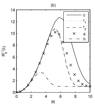
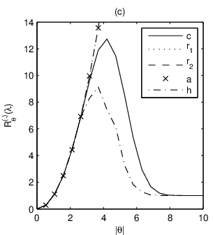
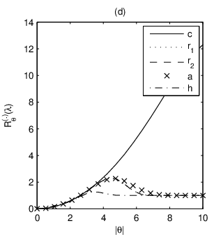
The risk of an individual coefficient using standard hard thresholding has been noted by Marron et al. [29], whilst the risk of the hyperanalytic thresholds are derived in appendix D, and is a special case of the bi-variate thresholding investigated by Fryzlewicz [14]. ∎For some examples of signal/noise distributions, the individual risk of a given coefficient is plotted in Figure 2 for the four estimation procedures using the universal threshold. Figure 2 (a) shows the reduced risk of ‘analytic’ thresholding compared to regular thresholding in 1-D when the means of the wavelet coefficient of the signal and of the HT of the signal are equal, and this then provides theoretical justification for the ‘analytic’ denoising procedure. Figures 2 (b), (c) and (d) show the risk associated with thresholding at any index using either the usual hard thresholding (), ‘analytic’ denoising (), Riesz denoising when () and () or Hypercomplex denoising (). The risk is calculated with and using the universal threshold. If the mean of the DWT of the quadrature components is of similar magnitude to the DWT of the signal then the risk is reduced. The greatest weakness of the proposed methods is if the means of the quadrature components are completely disparate from that of the original signal, as may be noted from figure 2 (c). The results of section III-B indicate that this will not be the case for typical image features. The norm of a signal and its HT are identical, and given the results of section III-B the means are unlikely to be consistently mismatched. Finally if there is no signal present we observe the following result.
Corollary 1 (The Risk of a Thresholded Coefficient when there is no signal )
The risk of an individual coefficient is using threshold strategy with for given by:
| (27) |
Proof:
See appendix D. We denote by
∎As the representation of the image will be sparse the risk if no signal is
present is important.
From the corollary, and the asymptotic forms in given in appendix D, we may note that the risk at the universal threshold when there
is no signal present is of the
same order for and
even if the coefficient differs in favour of
whilst and
correspond to different orders. The thresholds were introduced
to improve the estimation of signals that were slightly more spread across coefficients
than strictly necessary, but the risk for any coefficient when no
signal is present is of similar enough nature to make
the difference in estimation negligible (i.e. rather
than The examples will substantiate this
claim.
IV Examples
To examine the properties of the proposed methods, we have implemented simulation
studies on images that can be retrieved at http://sipi.usc.edu/database/
(Tiffany and Boat), whilst (Lenna and MRIScan) are downloaded from
http://www-stat.stanford.edu/~wavelab/. We used LA wavelets length 8.
To compare our results, similarly to [5],
we also implemented usual hard thresholding and the
Wavelet-domain Hidden Markov Model (HMM method) proposed by the Rice group
[13], where the
software is available at
http://www-dsp.rice.edu/software/, denoted by We used the
code with default settings, and
We implemented the method at several
Signal-to-Noise Ratio (SNRs) of 2 (very noisy), 4 and 8 (quite clean), with a set of images, i.e. Lenna ( version), Boat (), MRIScan ()
and the second channel of the colour image of Tiffany (). The SNR is (as usual) given
by Table I
shows the result over repeated simulations. Reduced Mean Square Errors
MSEs, and increased Peak Signal to Noise Ratios PSNRs (using the definition
of [30]), are observed when using the proposed method with
either hyperanalytic threshold criterion,
and the reduction
in MSE is of a respectable magnitude compared to variation across replications
as the estimated standard deviations in the MSEs are usually considerably smaller. Overall the hypercomplex thresholding
procedure is outperforming the Riesz thresholding as well as the other methods, apart from the boat image
at high SNRs where the HMM does better. The Hypercomplex method is expected
to outperform the Riesz method
from the risk calculations, but not perhaps from our discussion in sections
II-D and II-E. The Riesz transform may appear more useful
as it determines the prevalent direction
from the image, whilst the Hypercomplex transform simply decreases the risk
in estimation by considering variation associated with the same time-frequency
(i.e. 1-D)
behaviour in both axes separately, with the second variable treated as fixed. However, whilst the Riesz transform is
suitable to use on locally unidirectional structure as discussed in section
II-D, the hypercomplex transform
treats variation in both axes, and images quite frequently have multi-directional
variations present even locally. Some additional analysis of images has
also been implemented in [31].

Consider two cuts from reconstructions to further elucidate on these results: see Figure 1 (a)-(h). We show the hypercomplex reconstructions only as the Riesz and hypercomplex reconstructions are similar. Clearly both 1 (c) is more connected than (b), as is (g) to (f), whilst (d) and (h) has much remaining noise to preserve more detail. The proposed method performs quite well. In addition to the SNR’s chosen for the full range of images, we implemented the procedure at the SNR chosen by Starck et al. [5], namely adding Gaussian noise with a standard deviation of 20 to the raw Lenna image, or using a SNR of 5.58. The PSNR we observed in the noisy image (21.58) is less than theirs (22.13) but that is to be expected in noisy replications. We found for the methods tested in this paper that averaged over 100 replications (29.22), (30.12), (30.93) and (30.48), where they obtained for (28.35) and (30.80). Starck obtained PSNRs between 29.99 to 31.95 by using local ridgelets and curvelets. Clearly the hypercomplex denoising performs on par with the algorithms suggested, and in addition the proposed procedure is both cheap to implement and extremely simple to code.
| Example (SNR) | Boat (2/4/8) | Lena (2/4/8) | Tiffany (2/4/8) | MRIScan (2/4/8) |
|---|---|---|---|---|
| average MSE (n) | 95.4/23.8/6.0 | 95.4/23.8/6.0 | 95.4/23.8/6.0 | 381.5/95.4/23.8 |
| sd MSE (n) | 26.3/6.6/1.6 | 26.3/6.6/1.6 | 26.3/6.6/1.6 | 187.9/47.0/11.7 |
| PSNR (n) | 11.36/17.38/23.40 | 10.67/16.69/22.71 | 7.65/13.67/19.69 | 16.96/22.98/29.00 |
| average MSE (c) | 8.0/4.4/2.2 | 5.16/2.6/1.1 | 3.8/2.2/1.0 | 56.9/24.5/9.1 |
| sd MSE (c) | 6.7/3.2/1.2 | 7.3/2.3/0.8 | 4.9/2.5/0.8 | 110.0/43.4/15.3 |
| PSNR (c) | 22.12/24.68/27.70 | 23.34/26.34/29.88 | 21.64/24.02/27.39 | 25.22/28.88/33.18 |
| average MSE (r) | 7.1/3.8/1.8 | 4.5/2.2/0.93 | 3.4/1.9/0.8 | 46.9/19.7/7.3 |
| sd MSE (r) | 6.2/2.7/1.0 | 5.6/2.1/0.7 | 3.8/2.4/0.7 | 89.2/36.9/11.6 |
| PSNR (r) | 22.63/25.39/28.49 | 23.96/27.09/30.77 | 22.09/24.73/28.00 | 26.06/29.82/34.17 |
| average MSE (h) | 6.3/3.2/1.5 | 3.9/1.9/0.77 | 3.1/1.7/0.8 | 40.4/16.6/6.1 |
| sd MSE (h) | 6.6/2.2/0.9 | 4.6/2.0/0.6 | 3.3/2.3/0.6 | 79.1/31.0/8.7 |
| PSNR (h) | 23.14/ 26.04/29.2 | 24.56/27.74/31.58 | 22.48/25.06/28.55 | 26.71/30.57/34.92 |
| average MSE (hmm) | 6.7/3.0/1.4 | 6.3/2.1/ 0.85 | 5.4/1.8/0.8 | 48.9/20.9/7.5 |
| sd MSE (hmm) | 11.3/1.8/0.7 | 16.0/2.3/0.5 | 16.4/1.2/2.7 | 82.1/56.9/7.4 |
| PSNR (hmm) | 22.90/26.38/29.62 | 22.48/27.31/31.19 | 20.12/24.78/28.26 | 25.88/29.57/34.01 |
V Conclusions
This paper has proposed a new thresholding strategy for estimating decomposition coefficients, and has in particular implemented the strategy with the discrete separable DWT. We have determined the stochastic properties of the decomposition of the noise, and both the deterministic (for some stylized image features) and stochastic properties of the suggested new thresholding criterion. We established universal thresholds. We calculated the risk theoretically, and for some specific choices of the mean provided plots of the risk showing that the proposed methods outperform standard denoising theoretically. We implemented the procedure on several examples at several SNRs, comparing the methods with the Hidden-Markov-Model used by the Rice group as well as standard hard thresholding, and found that the proposed algorithms offered improvements in most cases. Given the simplicity in implementation, and visually pleasing reconstructions, hyperanalytic denoising methods offer a computationally cheap improvement to existing methodology, as well as offers insight into 2-D variational structure.
Acknowledgments
SO would like to express her thanks to the anonymous referees for the many helpful suggestions that substantially improved the paper, as well as her understanding of the topic. SO would also like to thank Professor Andrew Walden for introducing her to this research area, and gratefully acknowledges financial support from EPSRC (UK). SO gratefully acknowledges usage of WaveLab routines and the data sets.
References
- [1] D. L. Donoho and I. M. Johnstone, “Ideal spatial adaption via wavelet shrinkage,” Biometrika, vol. 81, pp. 425–455, 1994.
- [2] D. L. Donoho and I. M. Johnstone, “Adapting to unknown smoothness via wavelet shrinkage,” Journal of the Am. Stat. Assoc., vol. 90,pp. 1200-1224, 1995.
- [3] C. Stein, “Estimation of the Mean of a Multivariate Normal Distribution,” The Annals of Statistics, vol. 9, pp. 1135-1151, 1981.
- [4] T. R. Downie and B. W. Silverman, “The discrete multiple wavelet transform and threshold methods,” IEEE Trans. Signal Processing, vol. 46, pp. 2558-2561, 1998.
- [5] J. L. Starck, E. J. Candès and D. L. Donoho, “The curvelet transform for image denoising,” IEEE Trans. Image Processing, vol. 11, pp. 670-684, 2002.
- [6] D. L. Donoho, “Wedgelets: Nearly Minimax Estimation of Edges,” Annals of Statistics, vol. 27, pp. 859-897, 1999.
- [7] E. le Pennec and S. Mallat, “Sparse Geometric Image Representations,” IEEE Trans. Image Processing, vol. 14, pp. 423-438, 2005.
- [8] M. Jansen and A. Bultheel, “Empirical Bayes Approach to Improve Wavelet Thresholding for Image Noise Reduction,” J. Am. Stat. Assoc., vol. 96, pp. 629-639, 2001.
- [9] “Needles and Hay in Haystacks: Empirical Bayes Estimates of Possibly Sparse Sequences,” I. M. Johnstone and B. W. Silverman, Annals of Statistics,, vol. 32, pp. 1594-1649, 2004.
- [10] T. Cai and B. W. Silverman, Incorporating information on neighbouring coefficients into wavelet estimation”, Sankhyā Ser. B, vol. 63, pp. 127-148, 2001.
- [11] P. L. Dragotti and M. Vetterli, “Wavelet footprints: theory, algorithms and applications”, IEEE Trans. Signal Processing, vol. 51, pp. 1306-1323, 2003.
- [12] A. Pižurica and W. I. Philips and I. Lemahieu and M. Acheroy”, “A joint inter- and intrascale statistical model for Bayesian wavelet based image denoising,” IEEE Trans on Image Proc, vol. 11, pp. 545-557, 2002.
- [13] M. S. Crouse, R. Nowak and R. G. Baraniuk, “Wavelet-Based Statistical Signal Processing Using Hidden Markov Models,” IEEE Trans. Signal Processing, vol. 46, pp. 886-902, 1998.
- [14] P. Fryzlewicz, P.”, “Bivariate Hard Thresholding in Wavelet Function Estimation,” Statistica Sinica, to appear.
- [15] S. C. Olhede and A. T. Walden, “‘Analytic’ wavelet thresholding,” Biometrika, vol. 91, pp. 955-973, 2004.
- [16] S. C. Olhede and G. Metikas, The Hyperanalytic Wavelet Transform, Imperial College Statistics Section, TR-06-02, arXiv math.ST/0605623, 2006.
- [17] S. Mallat. A wavelet tour of signal processing, 2nd ed, Academic Press, New York, USA. 1999.
- [18] D. B. Percival and A. T. Walden, Wavelet Methods for Time Series Analysis, Cambridge University Press, Cambridge, UK, 2000.
- [19] B. Boashash, Note on the use of the Wigner distribution for time-frequency signal analysis, IEEE Trans. Accoust., Speech, Signal Proc, vol. 36, pp. 1518-1521, 1988.
- [20] G. Metikas and S. C. Olhede, Multiple Monogenic Morse Wavelets, Imperial College Statistics Section, TR-05-02, revised version to appear in IEEE Trans. Signal Proc., arXiv math.ST/0511324, 2005.
- [21] S. L. Hahn, Hilbert transforms in signal processing, Boston, MA, US, Artech House, 1996.
- [22] L. A. Vese & S. J. Osher, “Modeling Textures with Total Variation Minimization and Oscillating Patterns in Image Processing,” J. Scien. Comp., vol. 19, pp. 553–572, 2003.
- [23] M. Nielsen, “On the construction and frequency localisation of finite orthogonal quadrature filters,” J. of Approximation Theory, vol. 108, pp. 36–52, 2001.
- [24] R. A. Gopinath, “Phaselets of Framelets,” IEEE Trans. Signal Processing, vol. 53, pp. 1794–1806, 2005.
- [25] I. M. Johnstone and B. W. Silverman, “Wavelet Threshold Estimators for Data with Correlated Noise,” J. Royal Statistical Society B, vol. 59, pp. 319–351, 1997.
- [26] R. L. Dykstra, “Product inequalities involving the multivariate normal distribution,” J. Am. Stat. Assoc, vol. 75, pp. 646–650, 1980.
- [27] T. S. Ferguson, A Course in Large Sample Theory, Chapman & Hall/CRC, London, UK, 1996.
- [28] A. Grad and A. Solomon, “Distribution of Quadratic forms and some applications,” The Annals of Mathematical Statistics, vol. 26, pp. 464-477, 1955.
- [29] J. S. Marron and S. Adak, “Exact Risk Analysis Of Wavelet Regression,” J. Computational and Graphical Statistics, vol. 7, pp. 278–309, 1998.
- [30] S. Barber and G. P. Nason, “Denoising Real Images Using Complex-Valued Wavelets,” in Stochastic Geometry, Biological Structure and Images, Department of Statistics, University of Leeds, pp. 91-95, 2003.
- [31] S. C. Olhede, “Hyperanalytic denoising,” to appear at IEEE International Conference on Image Processing (ICIP), Atlanta, Georgia, October, 2006.
- [32] I. I. Gikhman and A. V. Skorokhod, The Theory of Stochastic Processes, Springer Classics in Mathematics, London, UK, 1980.
A: Digital Implementation
For future reference the Discrete Fourier Transform (DFT) and its inverse are given with by:
| (28) |
Note that the value of at frequencies is equivalent to the value of at frequencies and the equivalent statement mutatis mutandis hold for Let
and where we define:
We define in an analogous fashion. The digital definition of the filters corresponding to the three Hypercomplex components are defined via:
and Implementing the discrete HCT introduces an error term of
B: DWT of Typical Deterministic Image Features
We use period boundary treatment (see Mallat [17][p. 282–292]) when implementing the MODWT, so that with
| (29) |
Proof of Lemma 1
By direct calculation using equation (29):
and similarly whilst is introduced when is approximated by an exact band-pass structure.
Proof of Lemma 2
Proof of Lemma 3
Assume for simplicity of exposition, but with the necessary notational changes no such restriction needs to be made. Define the rotation matrix by and the change of variable given by: We assume that decays for large frequencies, and consider For example if then that as will concentrate to and with the rotated by version of with and then
The approximation in (1) relies on taking the form of a distribution contribution, i.e. constant over a large spatial domain, but a slowly varying will approximately yield the same result. Also we may find approximate descriptions for decomposition of the RTs, namely with and
| (30) | |||||
The approximation in (1) relies on the envelope being constant in the spatial domain – a slowly varying envelope will thus only approximately yield the same value, and this introduces an error term Similarly it transpires that and thus the result follows, with a new error term
Proof of Lemma 4
Also we may find approximate descriptions for the Hypercomplex components, namely:
| (31) | |||||
where the value of depends on the value of Similarly it transpires that and and are constants depending on the variability of
C: Statistics of the Normal Vector
For simplicity set when deriving the statistical properties
of the coefficients. has a spectral representation:
where
is a complex-valued orthogonal increment process, see
[32][p. 244], i.e.
if
The DWT is represented by subsampling
the MODWT:
noting that:
| (32) |
We have that and We approximate the magnitude of the wavelet filters as exact bandpass filters - see for example Nielsen [23] for a discussion of such approximations, and optimal filters to use. That is:
| (33) |
Proof of Propositions 1 & 2
The latter defining to be explicitly determined for and For where we determine that:
| (34) | |||||
by property 1 as is separable. Therefore
| (35) | |||||
Hence the total energy of the noise associated with the total magnitude square of the added quadrature components is a constant times the variance of the original signal.
Proof of Lemma 5
Given the noise was Gaussian and zero-mean we only need to determine the second order structure to deduce the Lemma, using equation (32).
Hence it follows that
| (36) |
and the two variances are obviously equal. Also:
| (37) |
Finally note that:
Clearly we can find the variance of the second RT by permuting the order of the spatial variable in the integration, and this then completes the variance calculations. From the proofs of propositions (1) and (2) we can note that the components of for are uncorrelated up to and this can also be shown by direct calculation, mutatis mutandis the calculations given above. Thus as was zero-mean Gaussian, and we are forming linear combinations to obtain the stated result follows from the expressions for the covariances of the components.
Proof of Lemma 6
a) First consider so that the variance of the two Riesz components is Then by Lemma 5 it follows directly that has a Moment Generating Function (MGF) given by and thus The probability that does not exceed is given by
| (38) | |||||
where the cdf be found in Grad & Solomon [28][p. 472], and the function is expanded as
b) Consider now Wlog assume that and otherwise relabel and suitably. If this collapses to the case given above. Define so that where the are iid Gaussian random variates with zero mean and unit variance, where Then the MGF is by Grad & Solomon [28]
with Defining and hence as we assumed we may note that and thus agrees with [28]’s notation. For future reference note that and we may rewrite Using results from Grad and Solomon we may determine:
For suitably defined constant From these formulae we can thus consider the probability of an observation exceeding a large threshold, which will be necessary for the selection of an appropriate threshold.
Proof of Lemma 7
We establish
These results follow trivially from the form of the partial HT [21]. From the proofs of propositions (1) and (2) we can note that the components of for a fixed value of are uncorrelated up to and this can also be shown by direct calculation mutatis mutandis the calculations given above.
Proof of Lemma 6
wavelet coefficients will be thresholded where magnitudes have the distribution given when and have the distribution that follows from where and so that by Dykstra [26]
ignoring terms in for suitably chosen constant if Thus with
if and we take
D: Risk Calculations
Proof of Theorem 1
We firstly note from [29][p. 293] that the risk of regular hard thresholding is given by
| (39) | |||||
We may then note that the risk for the hyperanalytic threshold with for where takes the value or is given by:
| (40) | |||||
Proof of Corollary 1
| (41) |
Furthermore the risk at can also be found for the other hyperanalytic thresholds. We note that for and denoted by in the Figures:
| (42) | |||||
whilst for denoted by
| (43) | |||||