The boundary Riemann solver coming from the real vanishing viscosity approximation
Abstract
We study the limit of the hyperbolic-parabolic approximation
The function is defined in such a way to guarantee that the initial boundary value problem is well posed even if is not invertible. The data and are constant.
When is invertible, the previous problem takes the simpler form
Again, the data and are constant. The conservative case is included in the previous formulations.
It is assumed convergence of the , smallness of the total variation and other technical hypotheses and it is provided a complete characterization of the limit.
The most interesting points are the following two.
First, the boundary characteristic case is considered, i.e. one eigenvalue of can be .
Second, as pointed out before we take into account the possibility that is not invertible. To deal with this case, we take as hypotheses conditions that were introduced by Kawashima and Shizuta relying on physically meaningful examples. We also introduce a new condition of block linear degeneracy. We prove that, if it is not satisfied, then pathological behaviours may occur.
2000 Mathematics Subject Classification: 35L65.
Key words: hyperbolic systems, parabolic approximation, initial boundary value problems, Riemann problem, conservation laws.
1 Introduction
The aim of this work is to describe the limit of the parabolic approximation
| (1.1) |
for . In the previous expression, the function is needed to have well posedness in the case the matrix is not invertible. The function is defined in Section 2. When the matrix is indeed invertible, system (1.1) takes the simpler form
| (1.2) |
Even if the equations in (1.1) and (1.2) are not necessarily in conservation form, nevertheless the conservative case
is included in the previous formulation. Indeed, one can define
In the present paper we assume that when the solutions converge, in the sense that will be specified in the following, to a unique limit . Since in both (1.1) and (1.2) the initial and boundary data are constant, then the limit solves a so called boundary Riemann problem, i.e. an hyperbolic initial boundary value problem with constant data. Results in [2] show that the study of boundary Riemann problems is a key point to determine the semigroup of solutions for an hyperbolic initial boundary value problem. We will came back to this point at the end of the introduction.
The goal of the work is to determine the value of for a.e. point . In particular, we determine the value of the trace of the limit on the axis . The reason why this is interesting is the following. Let us focus for simplicity on the case in which is invertible, i.e. on (1.2). It is known that, in general, the trace of the limit, which we denote by , is different from , the boundary datum imposed in (1.2). The relation between and is relevant for the study of hyperbolic initial boundary value problems and was first investigated (as far as we know) in [27]. Also, in [28] it was proved that the value of in general depends on the choice of the matrx . In other words, if in (1.2) one keeps fixed , and the function and changes only the matrix , then in general the value of will change, even if the system is in conservation form.
The most interesting points in the work are the following two. First, we cover the characteristic case, which occurs when an eigenvalue of the matrix can attain the value . The non characteristic case occurs when none of the eigenvalues of can attain the value . The characteristic case is more complicated to handle than the non characteristic one. Loosely speaking, the reason is the following. Suppose that the -th eigenvalue can assume the value . Then in the non linear case we do not know a priori if the waves of the -th family are entering or are leaving the domain.
The second point is that we cover the case of a non invertible viscosity matrix . To tackle this case we assume that the so called Kawashima Shizuta condition holds. We also introduce a new condition of block linear degeneracy. We provide a counterexample which shows that, if this condition is violated, then there may be pathological behaviours, in the sense that will be specified in the following.
The exposition is organized as follows. In Section 1.1 we give an overview of the paper, introducing the main ideas involved in the analysis. In Section 2 we discuss the hypotheses assumed in the work. In Section 3 we give a characterization of the limit of the parabolic approximation (1.2), i.e. when the viscosity matrix is invertible. Finally, in Section 4 we discuss the limit of (1.1) when the matrix is singular.
1.1 Overview of the paper
1.1.1 Section 2: hypotheses
Section 2 describes the hypotheses exploited in the work and it is divided into three parts.
Section 2.1 describes the hypotheses assumed in the case the matrix is invertible. These hypotheses were already considered in several previous works and they are automatically satisfied when the system admits a dissipative entropy.
In Section 2.2 we discuss the hypotheses assumed in the case the matrix is singular. These hypotheses can be divided into two groups.
The first group is composed by conditions that were already exploited in several previous works (e.g. in [34, 35, 36, 37, 47, 43, 44]). In particular one assumes that there exists a regular and invertible change of variables such that the following holds. If satisfies
then satisfies
| (1.3) |
The matrix has constant rank and admits the block decomposition
| (1.4) |
for a suitable . Also, and satisfy suitable hypotheses that are reasonable from the physical point of view since they were introduced in [34, 35, 36, 37] relying on examples with a physical meaning. In particular, we assume that the so called Kawashima Shizuta condition is satisfied.
Apart from these hypotheses, we introduce a new condition of block linear degeneracy, which is the following. Let
| (1.5) |
be the block decomposition of corresponding to (1.4), namely and belong to and and belong to . The condition of block linear degeneracy says that, for every given real number , the dimension of the kernel of is constant with respect to . In other words, the dimension of the kernel may vary as varies, but it cannot change when varies.
Block linear degeneracy is not just a technical condition. Indeed, in Section 2.2.2 we discuss counterxamples which show how, when the block linear degeneracy is violated, one can have pathological behaviors. More precisely, we exhibit examples in which block linear degeneracy does not hold and there is a solution of (1.3) which is not . These can be considered a pathological behaviour since one usually expects that the parabolic approximation has a regularizing effect.
On the other side, block linear degeneracy is not an optimal condition, in the following sense. It is possible to show that block linear degeneracy is satisfied by the Navier Stokes equation written using Lagrangian coordinates, but it is not satisfied by the Navier Stokes equation written in Eulerian coordinates. On the other side the two formulations of the Navier Stokes equation are equivalent, provided that the density of the fluid is strictly positive. This remark was first proposed by Frederic Rousset in [41] and it suggests that it is interesting to look for a condition strong enought to prevent pathological behaviours but at the same time sufficiently weak to be satisfied by the Navier Stokes equation written in Eulerian coordinates. This problem is tackled in the forthcoming paper [13].
In Section 2.2.1 it is defined the function ß which is used to define the boundary condition in (1.1). The point here is the following.
Consider an hyperbolic initial boundary value problem, and for simplicity let us focus on the conservative case:
| (1.6) |
It is known that if one assigns a datum (i.e. if one assigns boundary conditions), then the initial boundary value problem (1.6) may be ill posed, in the following sense. In general, there is no function which is a solution of
in the sense of distributions, which assumes the initial datum for and satisfies
for almost every . Also, it is know that a necessary condition to obtain a well posed problem is to assign a number of conditions on the boundary which is in general smaller then . Assume the boundary is non characteristic, i.e. assume that none of the eigenvalues of the jacobian can attain the value . In this case, one can impose on the boundary datum a number of conditions equal to the number of positive eigenvalues of .
We can now came back to the parabolic equation
| (1.7) |
Let us write , where , . Here is the rank of , as in (1.4). With this notations equation (1.7) can be rewritten as
| (1.8) |
Roughly speaking, the reason why one has to introduce the function ß is the following. Let be the number of strictly negative eigenvalues of the block , which itself is a matrix. Also, let denote the dimension of the kernel of . The second line in (1.8) contains a second order derivative of and hence can be seen as a parabolic component. On the other side, only first derivatives of appear and hence can be seen as an hyperbolic component. Actually, there is an interaction between the two components (this is ensured by the Kawashima-Shizuta condition). On the other side, because of the hyperbolic component one is not completely free to assign the boundary condition in (1.1). As pointed out in previous works (e.g in [43]) the number of conditions one can impose on the boundary is . Indeed, one can impose conditions on . On the other hand, one can impose on a number of conditions equal to the number of positive eigenvalues of , i.e. to . Summing up one obtains exactly .
Thus, the function in (1.1) takes values in and is a fixed vector in . The precise definition of is given in section 2.2.1 and it is such that the initial boundary value problem (1.1) is well posed. In Section 4.3 it is given a more general definition for the function ß.
Section 2.2.2 discusses three examples. The first two show that, if the condition of block linear degeneracy is violated, then there may be solution of
exhibiting pathological behaviors, in the sense explained before. More precisely, the first example deal with steady solutions
| (1.9) |
while the second one deals with travelling waves,
In the previous expression, represents the speed of the wave and it is a real parameter. Finally, the third example in Section 2.2.2 shows that if the rank of the matrix is not constant, then there may be solutions of (1.9) exhibiting pathological behaviours of the same kind discussed before.
Section 2.3 discusses the hypotheses that are assumed in both cases, when the matrix in (1.1) is invertible and when it is not. It is assumed that the system is strictly hyperbolic (see Section 2.3 for a definition of strict hyperbolicty). Also, it is assumed that when the solutions of of (1.1) converge to a unique limit. Also, it is assumed that the approximation is stable with respect to the initial and the boundary data and that the limit has finite propagation speed.
We refer to Section 2.3 for the exact statement of the hypotheses, here instead we underline another point. The proof of the convergence of in the case of a generic matrix is still an open problem. However, there are results that provide a justification of our hypotheses. In particular, in [28] it is proved the local in time convergence in the case is invertible, but in general different from the identity. Moreover, in [3] the authors proved the global in time convergence in the case of an artificial viscosity ( is identically equal to ). The analysis in [3] exploits techniques that were introduced in [8, 9, 10, 11] to deal with the Cauchy problem. In [3] it is proved the same kind of convergence we assume in the present properties. Also, other properties we assume here (stability of the approximation, finite propagation speed of the limit) are as well proved in [3]. Analogous results were proved in [48] for a special class of problems with boundaries.
Also, we point out that there are several works that study the stability of the approximation in the case of a very general viscosity matrix . Actually, the literature concerning this topic is very wide and hence we will quote only works that concern specifically initial boundary value problems: [47, 42, 43, 44].
1.1.2 Section 3: the characterization of the hyperbolic limit in the case of an invertible viscosity matrix
Section 3 discusses the characterization of the limit of (1.2) when the matrix is invertible. Actually, because of the hypotheses we assume in Section 2.1, we study the equivalent (in the sense specified therein) problem
| (1.10) |
Also, Section 3 is divided into fours parts.
Section 3.1 collects preliminary results that are needed in the following.
Section 3.2 gives a quick review of some results concerning the characterization of the limit in the Riemann problem. These results were introduced in [7].
The Riemann problem is a Cauchy problem with a piecewise constant inial datum with a single jump. Let us focus for simplicity on the conservative case:
| (1.11) |
A solution of (1.11) was first described in [39] assuming some technical hypotheses (i.e. that all the fields are either genuinely non linear or linearly degenerate). Since we will need in the following, here we briefly review the ideas exploited in [39] to obtain a solution of (1.11).
Denote by
the eigenvalues of the jacobian and by the corresponding eigenvectors. For simplicity, we assume that all the fields are genuinely non linear. In this case, one can chose the orientation of in such a way that . For every we denote by a curve in which is parameterized by and which enjoys the following property. For every value there exists a speed close to such that the Rankine Hugoniot condition is satisfied, i.e.
| (1.12) |
Also, let be the integral curve of starting at , in other words is the solution of the Cauchy problem
Finally, let be defined as follows:
In [39] it is proved that is a curve such that
In the following, we will say that is the i-th curve of admissible states. Indeed, every state can be connected to by either a rarefaction wave or a shock which is admissible in the sense of Liu. In other words, if then the solution of the Riemann problem
| (1.13) |
is
| (1.14) |
The meaning of the third line is that is equal to (the value assumed by the curve at the point ) when is exactly equal to evaluated at the point . The value of is well defined because of the condition .
On the other side, if then the solution of the Riemann problem (1.13) is
| (1.15) |
The speed satisfies the Rankine Hugoniot condition and it is close to .
In this way one obtains curve of admissible states , . To define the solution of the Riemann problem (1.11) one can proceed as follows. Consider the function
| (1.16) |
With the notation we mean that the starting point of is , i.e. that
It is proved in [39] that the map is locally invertible with respect to . In other words, the values of are uniquely determined if one imposes
at least if is a close enough to . One takes as in (1.11) and obtains the values . Indeed, we assume, here and in the following, . Once are known, one can obtain the limit gluing together pieces like (1.14) and (1.15).
The construction in [39] was extended in [40] to more general systems. Also, in [7] it was given a characterization of the limit of
| (1.17) |
when is sufficiently small (under hypotheses slightly different from the ones we consider here).
The construction works as follows. Consider a travelling profile for
i.e. such that
In the previous, expression, the speed of the wave is a real parameter. Then solves
| (1.18) |
The point is an equilibrium for (1.18). Also, one can prove that a center manifold around has dimension .
We recall here that every center manifold is invariant with respect to (1.18) and moreover satisfies the following property: let belong to and denote by the orbit starting at . Then
The constant in the previous expression is strictly positive, depends on the matrix and it is defined in Section 2 (Hypothesis 3).
Fix a center manifold . If is a solution to (1.18) laying on , then
| (1.19) |
The functions and are defined in Section 3.2.1.
The construction of works as follows. Fix and consider the following fixed point problem, defined on a interval :
| (1.20) |
We have used the following notations:
where
Also, denotes the concave envelope of the function :
One can show that the fixed point problem (1.20) admits a unique solution.
The link between (1.20) and (1.18) is the following: let satisfy (3.32). Assume that on and that . Define as the solution of the Cauchy problem
then is a solution to (3.31) satisfying
Thus, and are connected by a travelling wave profile.
On the other side, if on the interval , then the following holds. Consider , the integral curve of such that . Then lays on , thus and are connected by a rarefaction or by a contact discontinuity.
If , one considers a fixed problem like (1.20), but instead of the concave envelope of one takes the convex envelope:
Again, one can prove the existence of a unique fixed point .
The curve is defined setting
This curve contains states that are connected to by rarefaction waves and shocks with speed close to .
If , then the limit of the approximation (1.17) is
| (1.21) |
In the previous expression, is given by (1.20) and it is a monotone non increasing function.
It can be shown that in the case of conservative systems with only genuinely non linear or linearly degenerate fields the i-th curve of admissible states defined in [7] coincides with the one described in [39]. Once is known, then one defines as in (1.16) and find the limit gluing together pieces like (1.21).
In Section 3.2.2 we give a characterization of the limit of
| (1.22) |
when the boundary is not characteristic, i.e. when none of the eigenvalues of can attain the value . The idea is to costruct a locally invertible map which describes all the states that can be connected to , in the sense that is specified in the following. Loosely speaking, the map represents for the initial boundary value problem what the map defined in (1.16) represents for the Cauchy problem. Once is defined, one takes as in (1.22) and imposes
If and are sufficiently close, then this relation uniquely determines the values of . Once these values are known, then the limit is uniquely determined. More precisely, one can define the value of for a.e. . We will come to this point later.
The construction of the map works as follows. Denote by the eigenvalues of and by the associated eigenvectors. Also, assume that for every ,
In other words, is the number of negative eigenvalues of . These eigenvalues are real because this is one of the hypotheses listed in Section 2 (Hypothesis 3).
For consider the i-th curve of admissible states. Fix parameters and define
As before, the notation means that
the starting point of is
, .
Thanks to the results in [7] we quoted before, is connected to by a sequence of rarefaction waves and shocks with stricly positive speed.
To complete the construction, one considers steady solutions of
i.e. couples such that
| (1.23) |
The point is an equilibrium for (1.23). As shown in section 3.2.2, the stable manifold around has dimension , i.e. has dimension equal to the number of strictly negative eigenvalues of . Also, the following holds. Let be a map that parameterizes the stable manifold, then takes values into and it is defined on a space of dimension . To underline the dependence on we will write . Denote by the projection
Fix parameters and consider . Consider the problem
then there exists a unique solution of this problem such that
Setting , one finds a solution of
such that and for every ,
In this sense, we say that there is a loss of boundary condition when passing to the hyperbolic limit, because the boundary condition disappears in the limit. We point out that the idea of studying steady solutions to take into account the loss of boundary condition was already exploited in many previous work, e.g in [28].
To complete the characterization of the limit, we define as
In section 3.2.2 we prove that the map is locally invertible, i.e. the values of are completely determined is one sets
We take the same as in (1.22). As pointed out at the beginning of the paragraph, once are known, then the value of the self similar solution is determined for a.e. . One can indeed glue together pieces like (1.21). In particular, it turns out that the trace of on the axis is
As we have already underlined before, the relation between (the boundary datum in (1.22)) and is interesting for the study of hyperbolic initial boundary value problems.
In Section 3.2.3 we give a characterization of the limit of the parabolic approximation
| (1.24) |
when the boundary is characteristic, i.e. one eigenvalue of can attain the value . The characterization of the limit works as follows. We costruct a locally invertible map which describes all the states that can be connected to . Once is defined, one takes as in (1.24) and imposes
If and are sufficiently close, then this relation uniquely determines the values of . Once these values are known, then the limit is uniquely determined.
Formally, the idea is the same as in Section 3.2.2. However, the construction of the map is definitely more complicated in the boundary chararacteristic case.
Roughly speaking, the reason is the following. Let be the eigenvalues of . They are real by Hypothesis 3. Assume
where is a suitable positive constant. In other words, there are at least strictly negative eigenvalues, strictly positive eigenvalues and one eigenvalue close to .
Define
then is connected to by rarefaction waves and shocks with stricly positive speed. We now want to define the k-th curve of admissible states. To define , we might try to consider the fixed point problem
| (1.25) |
where , and are the same as in (1.20). However, if we consider (1.25) we are not doing the right thing. Indeed, we might have that the speed is negative at a certain point . Since eventually we want to define the limit as in (1.21), we want to be greater then .
Another problem is the following. Consider the system satisfied by steady solutions of
i.e. consider
| (1.26) |
Also, consider the equilibrium point . Let be the stable manifold of (1.26) around . For simplicity, assume . Then, there might be a solution such that
but does not belong to the stable manifold. However, this kind of solution should be taken into account when we study the loss of boundary condition.
To tackle these difficulties one can proceed as follows. Instead of the fixed point problem (1.25), one considers
| (1.27) |
In the previous expression, denotes the monotone concave envelope of the function ,
Some properties of the monotone envelope are discussed in Section 3.1.2, here we stress that is a concave and non decreasing function, thus the solution of (1.27) is always non negative.
Also, the following holds. Denote by the solution of (1.27) (existence and uniqueness are proved in Section 3.2.3). Define
| (1.28) |
and
Assume . Then is connected to by a sequence of rarefaction and shocks with positive speed. Also, one can show that there exists a steady solution ,
such that and
However, in general this solution does not belong to the stable manifold of system (1.26). This means that considering system (1.27) we also manage to take into account the converging steady solutions we were missing considering just the stable manifold of (1.26).
Heuristically, to complete the construction one should consider the stable manifold of (1.26) and hence take into account the steady solution that, for that goes to , converge to with fast exponential decay, in the sense specified in Section 3.2.3. Actually, the situation is more complex. The reason, loosely speaking, is the following . There may be a solution that converges to and such that some of its components converge with fast exponential decay, but other components converge more slowly. This possibility is not covered if we consider only the solutions laying on the stable manifold and those given by (1.27). To take into account this possibility some technical tools are introduced. More precisely, one considers suitable manifolds: center stable manifold and uniformly stable manifold. The existence of these manifolds is a consequence of results in [33], but some of the most important properties are recalled in Section 3.2.3.
Eventually, one manages to define a locally invertible function . One then takes as in (1.24) and imposes
If and are sufficiently close, then this relation uniquely determines the values of . Once these values are known, then the limit is uniquely determined and can be obtained gluing together pieces like (1.21). In particular, it turns out that the trace of on the axis is , where solves (1.27) and is given by (1.28).
1.1.3 Section 4: the characterization of the hyperbolic limit in the case of a singular viscosity matrix
In Section 4 we discuss the characterization of the limit of (1.1) when the matrix is not invertible. Actually, because of the hypotheses introduced in Section 2, one studies the limit of
| (1.29) |
This system is equivalent to (1.1) in the sense specified in Section 2.2. Also, : a precise definition is given Section 2. In particular, ß ensures that the initial boundary value problem (1.29) is well posed. Section 4 is divided into several parts.
In Section 4.1 we introduce some preliminary results. The point here is the following. In Section 3 we give a characterization of the hyperbolic limit when the viscosity matrix is invertible. A key point in the analysis is the study of travelling waves
| (1.30) |
and of steady solutions
| (1.31) |
To give a characterization of the hyperbolic limit when the viscosity matrix is not invertible, we have to study again systems (1.30) and (1.31). However, being the viscosity matrix singular, a technical difficulty arises. Let us focus, for simplicity, on the case of steady solutions. If is invertible, we can write
| (1.32) |
In this way, we write system (1.31) in an explicit form. On the other side, if the matrix is singular, additional work is required to reduce (1.31) in a form like (1.32). This is indeed done in Section 4.1. What we actually obtain is not a -dimensional first order system like (1.32), but a lower dimensional first order system. The exact dimension depends on the structure of the matrix , in the sense specified in Section 4.1.
In Section 4.2.1 we review the characterization of the hyperbolic limit in the case of a Riemann problem, i.e. the limit of
As for the case of an invertible (Section 3.2.1), the key point in the analysis is the description of the i-th curve of admissible states . However, there are technical difficulties due to the fact that is not invertible. Actually, in Section 4.2.1 we only give a sketch of the construction, and we refer to [7] for the complete analysis.
In Section 4.2.2 we introduce a technical lemma. The problem is the following. Consider a steady solution (1.31) and assume that it is written in an explicit form like (1.32). This is possible thanks to the considerations carried on in Section 4.1. Given an equilibrium point for this new system, consider the stable manifold around that equilibrium point. For reasons explained in Section 4.2, we need to know the dimension of this stable manifold. Lemma 4.7 ensures that the dimension of the stable manifold is equal to , where is the number of strictly negative eigenvalues of , is the number of strictly negative eigenvalues of the block and is the dimension of the kernel of the block . The block is defined by (1.5). Lemma 4.7 gives an answer to a question left open in [44].
In Section 4.2 we discuss the characterization of the hyperbolic limit of
| (1.33) |
when the matrix is singular, but the boundary is not characteristic, i.e. none of the eigenvalues of can attain the value .
To provide a characterization, we construct a map which enjoys the following properties. It takes values in and when vary it describes all that states that can be connected to , in the sense specified in the following. Note that similar functions are constructed in Section 3.2.2 and Section 3.2.3 and they are used to describe the limit of the parabolic approximation when the viscosity is invertible. However, in those cases the functions depend on variables, while in the case of a singular matrix the function depends only on variables.
Also, in the case of a singular viscosity we have to compose with the function ß, which is used to assign the boundary datum in (1.33). It is possible to show that the map is locally invertible, in other words the values of are uniquely determined if one imposes
| (1.34) |
provided that is small enough. We will plug the same as in (1.33). Once the values of are known, the limit can be determined a.e. in the same way as in Sections 3.2.2 and 3.2.3. In particular, one can determine exactly the value of the trace of the limit on the axis . As pointed out before, this is important for the study of hyperbolic initial boundary value problems.
The construction of the map works as follows. Denote as before by the number of the eigenvalues of that are strictly negative, since the boundary is not characteristic the number of strictly positive eigenvalues is . For , let be the i-th curve of admissible states, whose construction is reviewed in Section 4.2.1. Fix and define
| (1.35) |
As before, with the notation we mean that the starting point of is , i.e.
The value is connected to by a sequence of rarefactions and shocks with strictly positive speed.
To complete the construction, we consider steady solutions of
i.e. we consider solutions of
| (1.36) |
In Section 4.1.2 we discuss this system and we explain how to write it as first order O.D.E.. Also, in Section 4.2.2 we study the stable manifold of (1.36) around an equilibrium point such that and . In particular, we prove that this manifold has dimension . Let a map that parameterizes the stable manifold (we are also putting in evidence the dependence on ). For every there exists a solution of (1.36) such that and
setting one obtains a steady solution of
such that for every
In other words, we experience again a possibile loss of boundary condition from the parabolic approximation to the hyperbolic limit.
The map is then defined as follows:
In Section 4.3 we prove that is locally invertible with respect to .
Here, instead, we point out the following. The fact that the dimension of the stable manifold of 1.36 has dimension is proved in Section 4.2.2 and it is not, a priori, obvious. However, is exactly the number that makes things works if one wants the function to be locally invertible, in the sense that takes values in and hence to be locally invertible it should depend on variables. Since we have to take into account curve of admissible states, we are left with variables for the stable manifold.
In Section 3.2.2 we provide a characterization of the limit of
| (1.37) |
when the matrix is singular and the boundary is characteristic, i.e one of the eigenvalues of can attain the value . Actually this case requires no new ideas, in the sense that one can combine the techniques that are described in Section 3.2.3 (to deal with the fact that the boundary is characteristic) and in Section 4.2.3 (to deal with the singularity of the matrix ).
Finally, in Section 4.3 we introduce a technical lemma which guarantees that the function in (1.34) is locally invertible. We also provide a more general definition for the function ß. Such a definition still ensures that the initial boundary value problem (1.37) is well posed and that the map is locally invertible.
1.2 Unquoted references
Existence results for hyperbolic initial value problems were obtained in [31] and [45] relying on an adaptation of the Glimm scheme of approximation introduced in [29].
These results were later improved by mean of wave front tracking techniques. These techniques were used in a series of papers ([14, 15, 18, 19, 20, 21, 22, 23]) to establish the well posedness of the Cauchy problem. A comprehensive account of the stability and uniqueness results for the Cauchy problem for a system of conservation laws can be found in [16]. There are many references for a general introduction to system of conservation laws, for example [25] and to [46]. As concerns initial boundary value problems, in [1] the existence results in [31] and [45] were substantially improved, while well posedness results were obtained in [26].
In [2] it is studied the limit of the wave front tracking approximation. In particular, the authors extended to initial boundary value problems the definition of Standard Riemann Semigroup. Such a notion was introduced in [15] for the Cauchy problem. Roughly speaking, the analysis in [2] guarantees that to identify the semigroup of solutions it is enough to consider the behaviour of the semigroup in the case the initial and the boundary data are constant. It hence one of the most important motivations for the study of the parabolic approximation (1.1).
Acknowledgments: the authors express their gratitude to Denis Serre for having carefully read a previous version of the work and for his useful remarks. Also, the authors wish to thank Jeffrey Rauch for useful observations concerning the definition of boundary condition for the hyperbolic-parabolic system. Finally, we would like to thank Fabio Ancona for his useful remarks concerning the concave envelope of a function.
2 Hypotheses
This section introduces the hypotheses exploited in the work.
The exposition is organized as follows. In Section 2.1 we introduce the hypotheses we impose on system (1.2) when the viscosity matrix is invertible. In Section 2.2 we discuss the hypotheses exploited when the matrix in (1.1) is singular. Finally, in Section 2.3 we introduce the hypotheses needed in both the cases, when the matrix in (1.1) is invertible and when it is not.
In Section 2.2.1 we also discuss three examples which show that, if some of the conditions introduced are not satisfied, then there may be pathological behaviors, in the sense specified there. Also, we define the function used to assign the boundary condition in (1.1).
In [13] it will be discussed a way to extend to a more general setting the condition of block linear degeneracy, which is the third condition in Hypothesis 2.
2.1 The hypotheses assumed when the viscosity matrix is invertible
In this section it is considered the system
| (2.1) |
in the case the viscosity matrix is invertible. We assume the following.
Hypothesis 1.
There exists an (invertible) smooth change of variables such that (2.1) is equivalent to system
| (2.2) |
where
- 1.
for any , the matrix is real, symmetric and positive definite: there exists a constant such that
- 2.
for any , the matrix is symmetric.
- 3.
for any , the viscosity matrix is real and there exists a constant such that
In particular, the matrix may be the differential of the change of coordinates.
The initial boundary value problem (1.2) is equivalent to
| (2.3) |
where and . Indeed, one can verify that, thanks to the invertibility of the viscosity matrix, it is possible to assign a full boundary condition .
In the case system (2.1) is in conservation form
| (2.4) |
Hypothesis 1 is guaranteed by the presence of a dissipative and convex entropy.
For completeness we recall that the entropy is dissipative for (2.4) if for any there exists a constant such that
| (2.5) |
It is known (see for example [30]) that if system (2.1) admits a convex entropy , then there exists a symmetrizing and invertible change of variable . More precisely, if the inverse function is defined by , then satisfies system (2.2), with symmetric and given by
Moreover,
is symmetric (being the inverse of an hessian) and positive definite by convexity, while the dissipation condition (2.5) guarantees that
is positive definite. Hence Hypothesis 1 is satisfied.
2.2 The hypotheses assumed when the viscosity matrix is not invertible
The aim of this section is to introduce the hypotheses that will be needed in Section 4 to study system
| (2.6) |
in the case the viscosity matrix is singular.
Hypothesis 2.
There exists an (invertible) smooth change of coordinates such that (2.6) is equivalent to system
| (2.7) |
where
- 1.
the matrix has constant rank and admits the block decomposition
(2.8) with . Moreover, for every there exists a constant such that
- 2.
for any the matrix is symmetric. Moreover, the block decomposition of corresponding to (2.8) takes the form
(2.9) with , , and . Namely, only in the block depends on .
- 3.
a condition of block linear degeneracy holds. More precisely, for any the dimension of the kernel does not depend on , but only on .
This holds in particular for the limit cases in which the dimension of is equal to or to .
- 4.
the so called Kawashima condition holds: for any ,
- 5.
for any , the matrix is real, symmetric and positive definite: there exists a constant such that
In the following, we will denote by
(2.10) the block decomposition of corresponding to (2.8).
The change of variable guarantees that the initial-boundary value problem (1.1) is equivalent to
| (2.11) |
where , , .
Relying on the block decomposition of the viscosity matrix described in Hypothesis 2, in Section 2.2.1 the explicit definition of the function ß is introduced. Moreover, in Section 4.3 such a definition is extended to a more general formulation.
In order to justify the assumptions summarized in Hypothesis 2 it will be made reference to the works of Kawashima and Shizuta, in particular to [34] and to [37].
In particular, in [37] it is assumed that the system in conservation form
| (2.12) |
admits a convex and dissipative entropy which moreover satisfies
If one performs the change of variables defined by , finds that system (2.6) is equivalent to
with and symmetric.
It is then introduced the assumption
Condition N: the kernel of does not depend on .
and it is proved that Condition N holds if and only if there exists a change of variable which ensures that system (2.12) is equivalent to
for some that satisfies condition 5 in Hypothesis 2 and some and as in condition 2 and 1 respectively.
Moreover, it is shown that Condition N is verified in the case of several systems with physical meaning.
On the other side, the fourth assumption in Hypothesis 2 is the so called Kawashima condition and was introduced in [34]. Roughly speaking, its meaning is to ensure that there exists an interaction between the parabolic and the hyperbolic component of system (2.6) and hence to guarantee the regularity of a solution (2.6).
Examples 2.1 and 2.2 in Section 2.2.2 show that, if the condition of block linear degeneracy is violated, then one encounters pathological behaviours, in the following sense. One may find a solution of (2.6) that are not continuously differentiable. This is a pathological behaviour in the sense that, when one introduces a parabolic approximation, one expects a regularizing effect. In Section 1.1.1 we explain why it is interesting to look for an extension of the condition of block linear degeneracy to a more general setting. This problem will be tackled in [13].
Finally, Example 2.3 show that if the first condition in Hypothesis 2 is violated, then one can have pathological behaviours like the one described before. In other words, if the rank of can vary, then one may find a solution of (2.7) which is not continuously differentiable.
2.2.1 An explicit definition of boundary datum for the parabolic problem
Thanks to Hypothesis 2 system (1.2) is equivalent to
| (2.13) |
where . In this section we define the function ß. Once is known, one can obtain exploiting the fact that the map is invertible. In Section 4.3 we extend this definition to a more general setting.
Let be, as in the statement of Hypothesis 2, the rank of the matrix . Decompose as , where and . then the equation
can be written as
| (2.14) |
In the first line of (2.14) only first order derivatives appear, while in the second line there is a second order derivative . In this sense, can be regarded as the hyperbolic component of (2.14), while is the parabolic component. As explained in section 1.1.1, one can impose boundary conditions on , while one can impose on a number of boundary conditions equal to the number of eigenvalues of with strictly positive real part.
We recall that we denote by the number of strictly negative eigenvalues of , by the dimension of and by the number of strictly negative eigenvalues of . One can prove that the number of eigenvalues of with strictly negative real part is equal to (see Lemma (3.1) in Section 3.1.1, which was actually introduced in [6]). Also, the dimension of the kernel of is .
Let be an eigenvector of associated to an eigenvalue with non positive real part. Let be defined by
| (2.15) |
and finally let
Finally, let
where are the vectors of a basis in and are the eigenvectors of associated to eigenvalues with strictly positive real part.
Since , every can be written as
| (2.16) |
in a unique way.
We define ß as follows.
Definition 2.1.
We refer to Section 4.3 for an extension of this definition.
2.2.2 Examples
Example 2.1.
This example deals with the equation
| (2.18) |
in the case the condition of block linear degeneracy (the third in Hypothesis 2) does not hold.
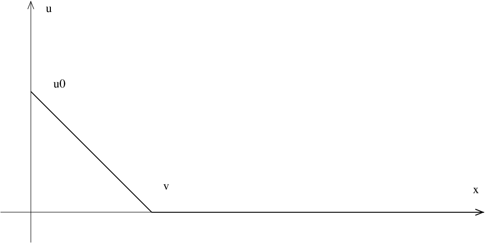
System (2.18) is satisfied by the steady solutions of (2.7). One therefore expects the solution of (2.18) to have good regularity properties: the example which is going to be discussed show that if the condition of block linear degeneracy does not hold a function satisfying (2.18) may have the graph illustrated by Figure 1 and hence be not . Moreover, the figure suggests that a pathological behavior typical of the solution of the porous-media equation may occur, namely it may happen that a solution is different from zero on a interval and then vanishes identically.
Let and let
and
Then the assumption of block linear degeneracy is not satisfied in a neighborhood of : we therefore impose the limit conditions
In this case equation (2.18) writes
| (2.19) |
Since the equation satisfied by admits more solutions in a neighborhood of , to introduce a selection principle we proceed as follows.
We consider a solution of (2.18) such that
The parameter is positive and we study the limit . Fix the initial datum . The component satisfies the Cauchy problem
| (2.20) |
If is sufficiently small then and hence is always negative. In other words, is a monotone non increasing function which satisfies for every . Also, note that if then, for every ,
| (2.21) |
This can be deduced by a comparison argument applied to the Cauchy problem (2.20). Indeed, if then
In particular, from (2.21) we deduce that for every is monotone decreasing with respect to and hence it admits limit .
Denote by the pointwise limit of for : we claim that satisfies
Indeed, let
If , then by monotoniticity for every and for every . Also, if is sufficiently small then and by monotonicity . Consider the relation
We take the limit and, applying Lebesgue’s dominated convergence theorem, we get
On the other side, if then by monotonicity . On the other side, for every . We conclude that if . In other words, and
This function ha the graph illustrated in Figure 1 and it is not continuously differentiable. In this sense, we encounter a pathological behaviour.
Remark 2.1.
An alternative interpretation of the previous considerations is the following.
Consider the family of systems
| (2.22) |
parametrized by the limit value . Let be the set of the values such that (2.22) admits a solution. The ODE satisfied by is
when . From a standard analysis it turns out that when , then . When , , while when , .
In other words, is a manifold of dimension when , a manifold with boundary and with dimension when , while when the dimension of the manifold drops to zero, i.e. the manifold reduces to a point.
Example 2.2.
Example 2.1 shows that, if the condition of blcok linear degeneracy (the third in Hypothesis 2) is not satisfied, then one can find a steady solution of
| (2.23) |
which is not continuously differentiable.
As we see in the following sections, steady solutions are important when studying the limit of the parabolic approximation (2.13). Other solutions that play an important role are travelling wave solutions, i.e such that
| (2.24) |
In the previous expression, is a real parameter and it is the speed of the travelling wave. More precisely, in the following sections we study travelling waves such that is close to an eigenvalue of the matrix .
Let
| (2.25) |
which are obtained from a system in conservation form
where
and is the constant matrix defined by (2.25).

The matrix defined by (2.25) has an eigenvalue identically equal to zero: we will focus on the travelling waves with speed .
System (2.24) can then be rewritten as
| (2.26) |
As in the case considered in Example 2.1, the condition of block linear degeneracy is not satisfied in a neighborhood of and therefore we study travelling wave solutions such that
From system (2.26) and from the previous condition one obtains
Hence in the following we ignore the third component of the solution and we study only the first two lines of the system, which can be rewritten as
| (2.27) |
If , the second line is equivalent to
Fix such that . We impose and we obtain
This solution can be extended as far as : when reaches the value zero, (2.27) admits more that one solution.
In order introduce a selection principle, we proceed as in Example 2.1 and we introduce a family of solutions of (2.24) such that
| (2.28) |
We also impose . In the previous expression, is a small and positive parameter and we study limit . One can repeat the same considerations as in the previous example and conlude that when the solution converges pointwise to
| (2.29) |
This function has the graph illustrated in Figure 2 and it is not continuously differentiable.
Example 2.3.
The aim of this example is to show that if in a system of the form (2.7) the rank of the matrix is not constant, thus contradicting the first assumption of Hypothesis 2, then pathological behaviors of the same kind described before may appear. More precisely, we find a steady solution which is not continuously differentiable.
We consider the system in conservation form
with
for some . In this case, the rank of drops from to when reaches : to find out pathological behaviors it seems therefore natural to study the solution in a neighborhood of . More precisely, the attention is focused on steady solutions
| (2.30) |
such that
| (2.31) |
and it will be shown that the graph of the first component has the shape illustrated in Figure 3. Hence is not continuously differentiable and presents a behaviour like the one typical of the solutions of the porous-media equation: it is different from zero on a interval and then vanishes identically.
In this case equation (2.30) writes
| (2.32) |
and hence after some computations one obtains
| (2.33) |
The equation satisfied by admits more than one solution in a neighborhood of .
To introduce a selection principle we consider the matrix
and the equation
| (2.34) |
In the previous expression, is a positive parameter and we study the limit . We keep the limit conditions (2.31) fixed. In other words, this time we do not perturb the limit condition (as in the previous examples), but the equation itself. Note that now is invertible. The solution of (2.34) with limit conditions (2.31) satisfies
| (2.35) |
Indeed, from
one obtains integrating
Multiplying the first line by and then integrating again one obtains (2.35). From (2.35) we get
Taking one eventually gets
Fix and consider the Cauchy problem
One can then exploit the same considerations as in the previous examples: in particular, the fact that for every is monotone decreasing with respect to follows from
if . One can the prove (proceeding as in the previous examples) that when , converges pointwise to a function satisfying
where
This function has the graph illustrated in Figure 3 and it is not continuously differentiable.

2.3 General hypotheses
This section introduces the general hypotheses required in both cases, i.e. when the viscosity matrix in (1.1) is invertible and when it is singular. In the statements of the hypotheses we actually make reference to the formulation (2.1) and (2.13). Thus, in particular, we consider the same value as in (2.1) and (2.13).
First of all, we assume strict hyperbolicity:
Hypothesis 3.
There exists such that, if belongs to a neighbourhood of of size then all the eigenvalues of the matrix are real. Moreover, there exists a constant such that
We also introduce an hypothesis of convergence:
Hypothesis 4.
Let
be a parabolic initial boundary value problem such that , and
| (2.36) |
For a suitable constant . Then we assume that there exists a time , which depends only on the bound and on the matrices , and , such that
We also assume directly a result of convergence and of uniqueness of the limit:
We point out that the uniqueness of the limit is actually implied by the next hypotheses and the uniqueness results for the Standard Riemann Semigroup with boundary: it is made reference to [2] for the extension of the definition of SRS to initial boundary value problems, while an application of this notion to prove the uniqueness of the limit of the vanishing viscosity solutions was introduced in [11] in the case of the Cauchy problem.
It is also assumed:
Hypothesis 5.
An hypothesis of stability with respect to perturbations in the initial and boundary data is also introduced:
Hypothesis 6.
There exists a constant such that the following holds.
Two families of parabolic initial boundary value problems are fixed:
| (2.37) |
with and in and satisfying the assumption (2.36).
Then for all and for all it holds
From the stability of the approximating solutions and from the convergence one can deduce the stability of the limit. More precisely, let and the limits of the two approximations defined above, then
Finally, it is assumed that in the hyperbolic limit there is a finite propagation speed of the disturbances:
Hypothesis 7.
There exist constants such that the following holds.
Let and in and bounded, let and be the solutions of (2.37) and and the corresponding limits. If
then
Analogously, if
then
Remark 2.2.
Hypothesis 7 may appear a bit technical. It implies the finite propagation speed of disturbances in the hyperbolic limit: an heuristic representation of this phenomenon is illustrated in Figure 4. Loosely speaking, the reason why we need finite propagation speed is the following. We have to be sure that the limit of (2.13) in the case of a generic couple of data can be obtained gluing together the limit one obtains in the case of cooked up data, namely data connected by travelling wave profiles.


3 Characterization of the hyperbolic limit in the case of an invertible viscosity matrix
The aim of this section is to provide a characterization of the limit of the parabolic approximation (1.1) when the viscosity matrix is invertible. The precise hypotheses that are assumed are listed in Section 2.1 and 2.3: in particular, these hypotheses guarantee that it is sufficient to study system
| (3.1) |
The exposition is organized as follows. In Section 3.1 we discuss some preliminary results. More precisely, in Section 3.1.1 we recall some transversality results discussed in [6]. In Section 3.1.2 we recall the definition of monotone envelope of a function and we introduce some related results. In Section 3.2 we review some results in [7]. Namely, we give a characterization of the limit of parabolic approximation
In Section 4.2.3 it is given a characterization of the limit of the parabolic approximation (3.1) in the case of a non characteristic boundary, i.e. when none of the eigenvalues of can attain the value . The case of a characteristic boundary occurs when one of the eigenvalues of can attain the value and it is definitely more complicated than the previous one. The characterization of the limit (3.1) in the case of a characteristic boundary is discussed in Section 3.2.3.
3.1 Preliminary results
3.1.1 Transversality results
The following lemma is discussed in [28]. However, for completeness we will repeat the proof.
Lemma 3.1.
Proof.
The first point is actually an immediate observation.
To simplify the notation, in the proof of the second point, we will write , and instead of , and respectively. One can define the continuous path
which satisfies the following condition: for every , is positively definite and hence invertible. Indeed,
| (3.2) |
Moreover, by classical results (see for example [38]) from the continuity of the path it follows the continuity of the corresponding paths of eigenvalues .
Let be the number of eigenvalues of with negative real part:
Because of the continuity of , to prove that the number of negative eigenvalues of is it is sufficient to prove that for any , cannot cross the imaginary axis. Moreover, the case is excluded because otherwise the corresponding eigenvector should satisfy for any and hence . It remains therefore to consider the possibility that is purely imaginary.
In the following, given a matrix we denote by the direct sum of all eigenspaces associated with eigenvectors with strictly negative real part, by the direct sum of the eigenspace associated with the eigenvector with zero real part, and the the direct sum of all eigenspaces associated with eigenvectors with strictly positive real part. Lemma 3.1 ensures that, if Hypothesis 1 holds, then for all
Thanks to the previous lemma, which is a direct application of Lemma 7.1 in [6], one can conclude that actually
| (3.4) |
3.1.2 Some results about the monotone envelope of a function
The aim of this section is to collect some results that will be needed in Section 3.2.3. Proposition 3.1 is very similar to results that were introduced, in a much more general form, for example in [5] and [32]. However, since the situation discussed here is slightly different, for completeness we give a proof. Also, results analogous to Propositions 3.2 and 3.3 are discussed in [4], but a proof is given here for completeness.
In the following, will denote the concave envelope of the function on the interval , namely
| (3.5) |
We will consider only the case of a function , i.e. and is Lipschitz continuous with Lipschitz constant smaller or equal to .
The symbol will denote the monotone envelope of the function on the interval , i.e.
| (3.6) |
.
Lemma 3.3.
Let , then
- 1.
is continuous and satisfies .
- 2.
If and
then is differentiable at and
- 3.
If and
then there exists such that such that
- 4.
, .
Proof.
By definition,
| (3.7) |
and hence . Moreover, the constant function is concave and greater or equal to and hence . Combining the two inequalities, one gets . Moreover, is a concave function and hence it is continuous in all the inner points of its domain, thus in . Later on we prove that it is also continuous at and .
To prove the second point, assume that and that . If , then thanks to (3.7)
and hence
Note that exists because , while
exists because the difference quotient is a monotone non increasing function. By the same reason,
Moreover, taking one can proceed as before and get
and hence putting all the previous considerations together one gets that exists and it is equal to .
To prove the third point, take such that and take and as follows:
and
To simplify the notations in the following we will also assume
the general case being analogous by subtracting a linear function.
First of all, note that for every because is a concave function and hence it is greater or equal to the segment joining two of its values. We want to prove that also . More precisely, we will consider the function
and we will prove that . Since the function is concave, it is enough to show that for every . By contradiction, assume that there exists such that . Assume that is exactly a point at which assumes it maximum on . If or then there is nothing to prove because for every in . Moreover, let denote a point at which the maximum of on is assumed: since is concave, then it is non decreasing for and non increasing for . Moreover, by (3.7) . Consider the function defined as follows:
where
and
Putting all the previous considerations together it turns out that and hence is a concave function which is greater or equal to . Thus, and hence in particular
This contradicts the assumption on .
Note that if , then automatically . Now we want to prove that, even if , . By contradiction, assume that , then consider the function
where is the point at which . Then is a concave function greater or equal to and hence , which contradicts the assumption .
In an entirely similar way one proves that even if . This completes the proof of the third point.
To prove the fourth point we proceed as follows. From the points and we know that is a bounded function that satisfies
Thus, it has bounded total variation and hence the following limit exists:
We want to prove . Let
The set is open and hence
for suitable sequences and .
If
there are two possibilities. If the infimum is actually a minimum, then
for some . One can then exploit the same function as before to prove that . If there exists a subsequence , then
Finally, if
then
then by the continuity of .
Analogous considerations guarantee that is continuous at and that . ∎
Because of points 2 and 3 of Lemma 3.3, the function is continuous at every point in . Also, relying on considerations analogous to those performed in the last part of the proof of Lemma 3.3, one can prove that is continuous at and . Note that it is actually enough to prove that the following limits exist:
Indeed, one can then apply the theorem of the limit of the derivative. We conclude that the following holds true:
Proposition 3.1.
If , then .
The following result describes the relation between the concave and the monotone envelope. The proof exploits considerations similar to those used to prove Lemma 3.3 and it will be therefore omitted.
Lemma 3.4.
Let , then
The value is given by
| (3.8) |
If is negative for every , then we set .
The following propostion collects some estimates that will be exploited in Section 3.2.3:
Proposition 3.2.
Let . Then
- 1.
- 2.
(3.9)
Proof.
To prove the first point, note that
because is a concave function greater or equal to . Thus, by the first point in Lemma 3.3,
and by analogous considerations
This concludes the proof of the first point.
To prove the second point, let us first make a preliminary consideration:
| (3.10) |
Indeed, if there is such that then and hence . In particular, if then on an interval and thus exploiting Lemma 3.3, point 2, one conclude with (3.10).
Let be a point at which the maximum of is assumed. Just to fix the ideas, suppose
Because of the second point in Lemma 3.3, if , then there are such that and
Moreover, since is non increasing, it is not restrictive to suppose . Also, because of the first point in the statement of Lemma 3.3, if then . Thus, if then . If then
Indeed,
and hence .
On the other side, if then combining (3.10) and the second part of Lemma 3.3 one gets that there exists such that
Moreover, . Indeed, if then and hence would be no more a point at which the maximum of is assumed. By Lagrange’s theorem, there exists such that
This concludes the proof of the second point in the case . The opposite case is entirely analogous. ∎
The following result concerns the dependence of the concave envelope from the interval:
Proposition 3.3.
Let , and assume that . Then there are constants and such that
| (3.11) |
and
| (3.12) |
Proof.
We will proceed in several steps:
- 1.
For every ,
(3.13) Indeed, the restriction of to the interval is a concave and non decreasing function which is also greater then . From (3.13) one deduces that, for every , the following implication holds:
(3.14) - 2.
- 3.
Before proving (3.11) we introduce other preliminary observations.
Given two arbitrary points and in , let the line
Then
(3.16) Indeed,
because is a concave function bigger than . On the other side,
since is a concave function bigger then .
- 4.
Define
If , then . Indeed, by contradiction assume that there exists a such that
(3.18) By (3.13) this implies that and hence, thanks to the third part of Lemma 3.3, there are and such that and on is a linear. Moreover, and Because of (3.14), this implies Also, because of the previous observation, it is not restrictive to assume . Since is a concave function, if and , then for every . If , then on and hence , which contradicts our hypothesis. On the other side, if then from and (3.14) we deduce Being a concave function, on is above the line joining and . Thus, in particular, , which contradicts (3.18).
- 5.
We now prove (3.11). Let as in the previous step. If , then and hence there are , such that and on is the linear interpolation between and . Relying on (3.16) , one can assume , getting on . Thus, and on . This implies
Since is the derivative of a concave function, then it is non increasing and
In particular, is non increasing on and hence its minimum on is assumed in . Thanks to the previous step,
which is equal to by the previous observations. By the forth part of Lemma 3.1, . To conclude, one can observe that
- 6.
Before proving (3.12) we introduce the following observations. Let such that . Then
(3.19) Indeed, consider for simplicity the case , . Let denote a point at which assumes its minimum and suppose, just to fix the ideas, that . Denote by the first derivative of : is Lipschitz continuous function with Lipschitz constant smaller than and such that .Thus, if . Moreover, Let us consider the Cauchy problem for at :
By a comparison argument one gets
(3.20) Moreover,
(3.21) To complete the proof of (3.19), let us consider to cases separately. If , consider the Cauchy problem
Then and thus the solution of
satisfies
(3.22) Define
By direct check one gets for every . Putting together (3.20), (3.21) and (3.22) one gets therefore
If then
(3.23) Indeed, thanks to (3.21) . Assume by contradiction that
(3.24) for some . Define
Since and , then there exits such that
Consider the Cauchy problem
then for . Then the solution of the backward Cauchy problem
satisfies for every . This contradicts (3.24) and hence (3.23) holds. One can then exploit the same function considered in the case and conclude.
- 7.
We now prove (3.12). Let be as in the previous steps, then on and hence
Thus,
(3.25) As in step 4, denote by and the values such that
As before it is not restrictive to assume and in this case
Since it is a non increasing function, the maximum in (3.25) is given by . Define
If , then for every
In particular, one has and hence . By the third part of Lemma 3.3
Now we can apply the previous step to defined on , thus obtaining
If , then . Consider two subcases separately. If , then also and hence because we are assuming . Then
On the other side, if one can proceed as follows. Since , and , then there exists such that . Then
We are now left to deal with the case . One then has
(3.26) Because of the implication (3.14), and hence . Moreover, , and on . Thus,
Since , there exists such that . Applying the previous step to the function defined on the interval , one gets . Inserting in (3.26), one gets
This concludes the proof of (3.12) and hence of the lemma.
∎
Proposition 3.4.
Let , and assume that . Then there are constants and such that
and
3.2 The hyperbolic limit in the case of an invertible viscosity matrix
3.2.1 The hyperbolic limit in the case of a Cauchy problem
In this section for completeness we will give a quick review of the construction of the Riemann solver for the Cauchy problem. We refer to [7] for the complete analysis. The goal is to characterize the limit of
| (3.27) |
The construction works as follows. Consider a travelling profile
then solves
| (3.28) |
Let be the -th eigenvalue of and let be the corresponding eigenvalue. If one linearizes the previous system around the equilibrium point one finds
The generalized eigenspace corresponding to the eigenvector is
It is then possible to define a center manifold which is parameterized by : we refer to [33] for an extensive analysis, here we will just recall some of the fundamental properties of a center manifold.
Every center manifold is invariant with respect to (3.28) and moreover satisfies the following property: let belong to and denote by the orbit starting at . Then
The constant is the separation speed defined in Hypothesis 3. A center manifold is defined in a neighbourhood of the equilibrium point and it is tangent to at .
Also, the following holds. Define
where are eigenvectors of different than . If we write , then the map
that parameterizes can be chosen in such a way that if is the projection from onto , then is the identity.
Fix a center manifold . Putting all the previous considerations together, one gets that a point belongs if and only if
| (3.29) |
Since all the equilibrium points lay on the center manifold, it turns out that when , then
Hence for all , for a suitable regular function . The relation (3.29) can be therefore rewritten as
Because of the tangency condition of the center manifold to the center space, it holds
Inserting the expression found for into (3.28), one gets
Considering the scalar product of the previous expression with one obtains
Hence setting
one can define
The fraction is well defined since and hence is strictly positive in a small neighborhood. The constant is as in the third condition in Hypothesis 1.
Thus,
Since
then
| (3.30) |
In the previous computations, we have exploited the symmetry of and and hence the fact that
Also, the constant in (3.30) is the same as in Hypothesis 1.
In conclusion, system (3.28) restricted to can be rewritten as
| (3.31) |
One actually studies the following fixed point problem, defined on a interval :
| (3.32) |
We have used the following notations:
where
Also, denotes the concave envelope of the function :
The link between (3.32) and (3.28) is the following: let satisfy (3.32). Assume that on and that . Define as the solution of the Cauchy problem
then is a solution to (3.31) satisfying
Thus, and are connected by a travelling wave profile.
As shown in [7], (3.32) admits a unique continuous solution . Also, one can show that and are connected by a sequence of rarefaction and travelling waves with speed close to . If is the limit of
then as
| (3.33) |
The -th curve of admissible states is defined setting
If , one considers a fixed problem like (3.32), but instead of the concave envelope of one takes the convex envelope:
Again, one can prove the existence of a unique fixed point .
Also, in [7] it is proved that the curve is Lipschitz continuos with respect to and it is differentiable at with derivative given by . Moreover, the function is Lipschitz continuos with respect to .
Consider the composite function
With the previous expression we mean that the starting point for is not but . Thanks to the previous steps, the map is Lipschitz continous with respect to and differentiable at , . The column of the jacobian are . Thus the jacobian is invertible and hence, exploiting the extension of the implicit function theorem discussed in [24] (page 253), the map is invertible in a neighbourhood of . In other words, if is fixed and is sufficiently close to , then the values of are uniquely determined by the equation
Taking the same as in (3.27), one obtains the parameters which can be used to reconstruct the hyperbolic limit of (3.27). Indeed, once are known then can be obtained gluing together solutions like (3.33).
3.2.2 The hyperbolic limit in the non characteristic case
The goal of this section is to provide a characterization of the limit of the parabolic approximation (3.1) in the case of a non characteristic boundary, i.e. when none of the eigenvalues of can attain the value . More precisely, we assume the following.
Hypothesis 8.
Let be the eigenvalues of the matrix . Then there exists a constant such that for every
| (3.34) |
Thus, in the following will denote the number of eigenvalues with strictly negative negative real part and the number of eigenvalues with strictly positive real part.
To give a characterization of the limit of (3.1) we will proceed as follows. We wil construct a map which is a boundary Riemann solver in the sense that as vary, describes states that can be connected to . We will the show that the map is locally invertible. Hence, given and sufficiently close, the values of are uniquely determined by the equation
Once are known the limit of (3.1) is completely characterized. The construction of the map is divided in some steps:
- 1.
Waves with positive speed
- 2.
Boundary layers
We have now to characterize the set of values such that the following problem admits a solution:
We have thus to study system
(3.35) Consider the equilibrium point , linearize at that point and denote by the stable space, i.e. the eigenspace associated to the eigenvalues with strictly negative real part. Thanks to Lemma 3.1, the dimension of is equal to the number of negative eigenvalues of , i.e. to . Also, is given by
where are the eigenvalues of with negative real part and are the corresponding eigenvectors.
Denote by the stable manifold, which is parameterized by . Also, denote by a parameterization of :
Let be the projection
If for some , then system (3.35) admits a solution. Note that thanks to classical results about the stable manifold (see eg [33]) the map is differentiable and hence also is differentiable. In particular, the stable manifold is tangent at to and hence the columns of the jacobian of computed at are .
Note that the map actually depends also on the point and it does in a Lipschitz continuos way:
- 3.
Conclusion
Define the map as follows:
(3.36) From the previous steps it follows that is Lipschitz continuos and that it is differentiable at . Also, the columns of the jacobian are . Thus, thanks to Lemma 3.1, the jacobian is invertible. One can thus exploit the extension of the implicit function theorem discussed in [24] (page 253) and conclude that the map is invertible in a neighbourhood of . In particular, if one takes as in (3.1) and assumes that is sufficiently small, then the values of are uniquely determined by the equation
(3.37) Once the values of are known, then the limit can be reconstructed. In particular, the trace of on the axis is given by
(3.38) The self similar function is represented in Figure 5 and can be obtained gluing together pieces like (3.33) .

Theorem 3.1.
Let Hypotheses 1, 3, 4, 5, 6 , 7 and 8 hold. Then there exists small enough such that the following holds. If , then the limit of the parabolic approximation (3.1) satisfies
for a suitable vector . The map is defined by (3.36). Given and , one can invert and determine uniquely . Once are known one can determine a.e. the value assumed by the limit function. In particular, the trace of the hyperbolic limit in the axis is given by (3.38).
3.2.3 The hyperbolic limit in the boundary characteristic case
The aim of this section is to provide a characterization of the limit of the parabolic approximation (3.1) when the matrix is invertible, but the boundary is characteristic, i.e. one eigenvalue of can attain the value .
Let be the bound on the total variation introduced in Hypothesis 4. Moreover, as in the previous section we will denote by the eigenvalues of the matrix . The eigenvalue is Lipschitz continuous with respect to and hence there exists a suitable constant such that, if , then for every in a neighbourhood of of size , . Thus, in particular, if then Hypothesis 8 is satisfied for some and hence the boundary is non characteristic. In this section we will therefore make the following assumption:
Hypothesis 9.
Let the same constant as in Hypothesis 4 and let the constant introduced before. Then
| (3.39) |
Note that, because of strict hyperbolicity (Hypothesis 3) the other eigenvalues of are well separated from zero, in the following sense: there exist a constant such that for all satisfying , it holds
| (3.40) |
The notation used in this section is therefore the following: denotes the number of strictly negative eigenvalues of , while is the number of strictly positive eigenvalues.
The study of the limit is more complicated in the boundary characteristic case than in the case considered in the previous section. The main ideas exploited in the analysis are described in the introduction, here instead we will give the technical details of the construction. As in the previous section, the characterization of the limit will be as follows: we will construct a map which describes all the states that can be connected to . We will then show that the map is locally invertible: thus, given and sufficiently close, the values of are uniquely determined by the equation
Once are known one can proceed as in the previous section and determine a.e. the value assumed by the limit function. The construction of the map will be given in several steps:
- 1.
Study of the waves with uniformly positive speed
Consider the Cauchy datum , fix parameters and consider the value
The curves are, as in Section 3.2.1, the curves of admissible states introduced in [7]. The state is then connected to by a sequence of rarefaction and travelling waves with uniformly positive speed. The speed is uniformly positive in the sense of (3.40).
- 2.
Reduction on the center stable manifold
Consider system
(3.41) and the equilibrium point . Linearizing the system around one obtains
(3.42) Thanks to (3.40), the matrix has 1 null eigenvalue and strictly negative eigenvalues. Because of Lemma 3.1 one can then conclude that the matrix (3.42) has null eigenvalues and eigenvalues s with strictly negative real part..
Let be the kernel of (3.42), the eigenvspace associated eigenvalues s with strictly negative real part. and the eigenspace associated to eigenvalues s with strictly positive real part. There exists a so called center stable manifold which is parameterized by : we refer to [33] for an extensive analysis, here we will just recall some of the fundamental properties of a center stable manifold. If we write , then the map
that parameterizes can be chosen in such a way that if is the projection from
onto , then is the identity.Every center stable manifold is invariant with respect to (3.41) and moreover satisfies the following property: let belong to and denote by the orbit starting at . Then
The constant is the separation speed defined in (3.40). We are also assuming that is bigger than : this is a consequence of Hypothesis 9 provided that is sufficiently small. A center stable manifold is defined in a neighbourhood of the equilibrium point and it is tangent to at .
In the following, we will fix a center stable manifold and we will focus on the solutions of (3.41) that lay on . The center and the stable space of (3.42) are given respectively by
and
In the previous expression, is a unit vector in the kernel of , while are the eigenvectors of associated to the eigenvalues s with strictly negative real part. Since is the identity, then a point belongs to the manifold is and only if
where are the eigenvectors of associated to eigenvalues with strictly positive real part.. Since all the equilibrium points belong to the center stable manifold, then we must have when are all . Thus, since are linearly independent, for all and for every and . This means, in particular, that for every there exists a -dimensional vector such that
Define
then a point belongs to if and only if
(3.43) where denotes . Since is tangent to at , then
Plugging into system (3.64) one gets
(3.44) Moreover, the matrix
satisfies
Hence (3.44) can be rewritten as
(3.45) Since
then the columns of are linearly independent in a small enough neighbourhood. Thus one can find a matrix such that
Multiplying (3.45) by one finds
(3.46) Define
(3.47) then by construction is a diagonal matrix with one eigenvalue equal to and eigenvalues with strictly negative real part. Also, if and , then
(3.48) for a suitable strictly positive constant . This is a consequence of conditions 1 and 3 in Hypothesis 1.
- 3.
Analysis of the uniformly stable component of (3.49)
Linearizing system (3.49) around the equilibrium point one obtains the matrix
(3.50) which has distinct eigenvalues with strictly negative real part and the eigenvalue with multiplicity . Also, the manifold
is entirely constituted by equilibria.
Then there exists a uniformly stable manifold which is invariant for (3.49) and is characterized by the following property: given belonging to , denote by the solution of (3.49) starting at . Then there exists a point belonging to such that
We remark that the uniformly stable manifold is contained but in general does not coincide with a given center stable manifold. Indeed, does not contain, for example, the trajectories that converge to a point in with speed slower than .
The existence of the uniformly stable manifold is implied by Hadamard-Perron theorem, which is discussed for example in [33]. The application of the uniformly stable manifold to the study of hyperbolic initial boundary values problems is derived from [3]. In our case, the existence of the uniformly stable manifold is loosely speaking guaranteed by the strict hyperbolicity of (Hypothesis 3), namely the fact that the eigenvalues of are uniformly separated one from each other. In the following, we will just recall some of the properties of the uniformly stable manifold.
Let
where are as before the eigenvectors of and are the vectors of the canonical basis of , and so on. The uniformly stable manifold is parameterized by and hence has dimension . The parameterization
can be chosen in such a way that the following property is satisfied. Let
If we write as and we denote by the projection onto , then we can have equal to the identity.
By considerations analogous, but easier, to those performed to get (3.43) one deduces that a point belongs to if and only if
where are the components of along . The matrix belongs to and
We want now to compute . Plugging the relation into (3.49) one gets
(3.51) where is a matrix such that for every and . Thus,
for a suitable matrix such that is a diagonal matrix with all the eigenvalues with strctly negative real part. Plugging back into (3.51) one gets
(3.52) - 4.
Analysis of the center component of (3.49)
Linearizing system (3.49) around the equilibrium point one obtains (3.50) and hence the center space is given by
Consider the center manifold , parameterized by : thanks to considerations similar, but easier, than those performed in the previous steps one gets that a point belongs to if and only if
where and .
Again, with considerations analogous, but easier than those performed at the previous step one gets
(3.53) for a suitable function satisfying Also, thanks to (3.48),
(3.54) - 5.
Decomposition of (3.49) in center and uniformly stable component
In this step, we will fix a trajectory of (3.49) and we will decompose it in a uniformly stable and in a center component, in the following sense. We exploits the manifolds and introduced in the previous steps and we decompose
(3.55) Plugging this expression into the first line of (3.49) one gets
From the second line of (3.49) one gets
One can prove that
for a suitable matrix which satisfies for every and (the same as in the previous step). Thus, exploiting (3.52) and (3.53), we get
(3.56) The functions and satisfy
and hence in a neighbourhood of the columns of and are all linearly independent. Denote by the vectors of the dual basis and define
Then multiplying (3.56) on the left by one gets
where is given by
The matrix is diagonal and all the eigenvalues have strictly negative real part.
To study system (3.57) we will first consider the solution of (3.57) when and . Fix : we will actually study the following fixed point problem, which is defined on the interval :
(3.59) In the previous expression,
(3.60) where
(3.61) The constant is defined by (3.58).
If , one considers a fixed problem like (3.59) but instead of the monotone concave envelope of one takes the monotone convex envelope:
In the following we will consider only the case , the case being entirely similar.
The link between system (3.59) and system (3.57) in the case , is the following. Let solve (3.59), assume that and define
(3.62) Let
in the following we will prove that if and only if .
The function solves (3.57) in the case , . If then is also a trivial solution of (3.57) in the case , and the following properties are satisfied. Note that the function is a steady solution of the original parabolic equation since :
Moreover,
(3.63) From system (3.59) we also get that is connected to by a sequence of rarefaction waves and shocks with non negative speed.
- 6.
Analysis of the purely center component
The purely center component is the solution of system (3.59).
Lemma 3.5.
Fix such that . Then system (3.59) admits a unique solution satisfying
- (a)
, , is Lipschitz with constant .
- (b)
, , is Lipschitz with constant .
- (c)
, , is Lipschitz with constant .
The constants , , , , and do not depend on . The function defined by (3.60) belongs to for a suitable constant which again does not depend on .
The symbol denotes the space of functions such that is Lipschitz continuous and has Lipschitz constant .
Proof.
The proof of the lemma relies on a fixed point argument. Only the fundamental steps are sketched here.
Define
(3.65) In the previous expression, is defined as follows:
for a suitable constant whose exact value does not depend on and will be determined in the following. Also the constants , , , and do not depend on and their exact value will be estimated in the following.
If then the function defined by (3.60) satisfies for a large enough constant . Moreover, exploiting (3.39) and (3.61), one gets
(3.66) if is sufficiently small and sufficiently large.
The same computations ensure that
(3.67) for a large enough . Finally,
(3.68) for a sufficiently large constant . In the previous estimate, we have exploited the following observation: since by (3.58)
then
(3.69) Because of (3.66), (3.67) and (3.69), and hence by Proposition 3.2 . Moreover,
One can then conclude that the map defined by the right hand side of (3.59) maps into itself.
Choosing large enough (but independent from ) it is possible to prove the contraction property. One has to exploit all the previous estimates and also properties (3.9) and (3.69), which are needed to handle the second and the third component of .
It turns out that the Lipschitz constant of (i.e., the constant in the contraction) is uniformly bounded with respect to .
∎
In the following it will be useful to know how the solution of (3.59) depends on the length of the interval of definition. More precisely, in order to underline the dependence from , we will denote the first component of the solution of (3.59) as . Let
where the dependence from the initial point is also made explicit.
To study how depends on we will exploit the following result:
Lemma 3.6.
Fix and let , such that . Let and be the corresponding solutions of (3.59). Then,
(3.70) where is a suitable constant which does not depend on .
Proof.
In the following we will denote by and the maps defined by the right hand side of (3.59) when and respectively. Moreover, to simplify notations, we will denote by the restriction of the fixed point of to the interval .
Since is the fixed point of , one then has
In the previous formula, denotes the Lipschitz constant of , which turns out to be uniformly bounded with respect to as underlined in the proof of Lemma 3.5. Moreover, and denote the spaces defined by (3.65) when .
Thus, to prove the lemma one actually reduces to prove
In the previous formula, , and denote respectively the first, the second and the third component of .
Since is the fixed point of , then
Hence, to prove the lemma it is sufficient to show that
and that
This follows directly from Proposition 3.4. ∎
In particular, the previous Lemma implies that
(3.71) Indeed, assuming for example that , one can write
Take in the previous estimate: since
(3.72) one gets
(3.73) Thus, the function defined before is differentiable at and the gradient is the eigenvector .
The function depends Lipschitz continuously on too:
Lemma 3.7.
Fix such that . Take such that for a certain constant . If , then
(3.74) for a suitably large constant .
Proof.
The value is the fixed point of the application defined by (3.59). To underline the dependence of on we will write
The map depends Lipschitz continuously on , but one cannot apply directly the classical results (see e.g. [17] ) on the dependence of the fixed point of a contraction from a parameter because of a technical difficulty. Indeed, the domain of the contraction depends on .
To overcome this problem, one can proceed as follows. Define and the spaces defined as in (3.65) with and respectively. If is the fixed point of the application defined on , then
Choosing , one gets that belongs to . Thus,
In the previous expression, is the fixed point of the application . One can then proceed as in [17] and conclude that
(3.75) ∎
- (a)
- 7.
Analysis of the purely stable component
The purely center component satisfies (3.64).
Lemma 3.8.
Proof.
We know that is has eigenvalues . Relying on (3.34), one obtains
Moreover, if and , then
where denotes (here and in the following) some constant that depends neither on nor on .
The columns of are the eigenvectors , which are all unit vectors. Thus, if and , then
From the previous observations one gets that the application defined by (3.64) maps into itself.
To prove that the application is a contraction, take and . Then
Choosing sufficiently small, one can suppose that in the previous expression. Moreover, one can suppose that is small enough to have that , .
Finally,
Assuming that is small enough, and . Thus the map is contraction and the constant of the contraction is less or equal to uniformly for . ∎
The solution of (3.64) depends on the parameter . The regularity of with respect to is discussed in the following lemma.
Lemma 3.9.
Fix and let , two initial data such that , . Let and the corresponding solutions of (3.64). Then,
(3.77) where is a suitable constant which does not depend on . Moreover, if , then . Also,
(3.78) Equation (3.78) guarantees, in particular, that the application
is differentiable with respect to when and that the jacobian is the matrix , whose columns are the eigenvectors .
Proof.
Let the application defined by the right hand side of (3.64). To underline the dependence on the parameter , we write
and denote by and respectively the first and the second component of . For every ,
and
Hence, (3.77) holds with , where is the Lipschitz constant of and hence it is smaller than because is a contraction. Moreover, from the proof of Lemma 3.8 it follows that is bounded away from uniformly with respect to . This concludes the proof of the first part of the lemma.
To prove the second part, we observe that
and that
Hence,
This completes the proof of the lemma. ∎
To study the dependence of on one can proceed as follow. Fix close enough and denote by and the solution of (3.64) corresponding to and respectively. Then classical results (see e.g. [17]) on the dependence of the fixed point of a contraction on a parameter ensure that
(3.79) for a suitable constant . In particular,
(3.80) - 8.
The component of perturbation
Indeed, for it holds
and hence
Let
the inverse function of , . If , we set for every .
The component of perturbation is the fixed point of the transformation
(3.81) In the equation for we used the same notation as in (3.64):
Lemma 3.10.
Let and be as in Lemma 3.5 and 3.8 respectively. Then there exists a unique solution of (3.81) belonging to , where the spaces , and are defined as follows:
and
In the previous expressions, the constants and do not depend on .
The space is endowed with the norm
where is a suitable constant which does not depend on . The spaces and are endowed respectively with the norms
and
Proof.
It is enough to prove that the right hand side of (3.81) defines a contraction on . As in the proof of Lemma 3.8, one observes that is a diagonal matrix with all the eigenvalues less or equal to . Thus,
Moreover, from Lemma 3.8 one gets that for every ,
Another useful observation is the following:
(3.82) Indeed, if , then one can exploit the change of variable . Recalling that is the inverse function of , which is defined by (3.62), one has
If , then and hence (3.82) is trivial.
One can also assume
(3.83) and hence
Moreover, it holds
Since this follows from the regularity of and from the estimates
Exploiting the previous observations, by direct check one gets that the right hand side of (3.81) belongs to .
To prove that the map is actually a contraction, one has to exploit again the previous remarks, combined with the following: for every ,
and
One can then check that the map is a contraction, provided that is sufficiently small. ∎
Since and depend on the parameters and respectively, then also does. Let
The following lemma concerns the regularity of with respect to .
Lemma 3.11.
The function is differentiable with respect to at and the jacobian is the null matrix.
Also, let and such that , . Then,
(3.84) Proof.
By construction,
(3.85) This implies the differentiability at .
To prove the second part of the lemma, we will focus only on the dependence from and . The proof of the Lipschitz continuous dependence from is completely analogous.
We can observe that is the fixed point of a contraction , defined by the right hand side of (3.81). To underline the dependence from we write
and denote by , and respectively the first, the second and the third component of . Since the Lispchitz constant of is not only smaller than but also bounded away from uniformly with respect to , then to prove (3.84) it is enough to prove that, for every ,
(3.86) Let
and and the inverse functions. Just to fix the ideas, let us assume that , then . Exploiting Lemma 3.6 one gets that, as far as , it holds
and hence
(3.87) If , then
where
Thus, estimate (3.87) still holds.
To prove (3.86), the most complicated terms to handle are in the form
(3.90) Exploiting (3.89) the first term in the previous sum can be estimated as follows:
where we have supposed that is small enough to obtain .
To handle with the second term in (3.90) one can observe that
Moreover,
By analogous considerations, one can conclude that the second term in (3.90) can be bounded by .
One can also perform similar estimates on all the other terms that appear in
and
and conclude that (3.86) holds. ∎
Set and define
| (3.91) |
Combining (3.70), (3.77) and (3.84) one gets that is Lipschitz continuous with respect to :
| (3.92) |
for a suitable constant .
Moreover, is differentiable at because of (3.73) , (3.78) and (3.85). The colums of the jacobian matrix are the eigenvectors .
Finally, is also Lipschitz continuous with respect to , namely
| (3.93) |
Define
| (3.94) |
We recall that the composite map is Lipschitz continuous and differentiable at , with the columns of the jacobian given by the eigenvectors . This was proved in [7].
Combining this with (3.93) and (3.94) one gets that is Lipschitz continuous. Moreover, it is differentiable at and the columns of the jacobian are the eigenvectors . Thus, thanks to (3.4), the jacobian is invertible and hence, exploiting the extension of the implicit function theorem discussed in [24] (page 253), the map is invertible in a neighbourhood of .
Thus, if is fixed and is sufficiently close to , then the values of are uniquely determined by the equation
| (3.95) |
We will take equal to the boundary datum imposed on the parabolic approximation (3.1). Once are determined one can determine the values of the hyperbolic limit a.e. . This can be done glueing together pieces like (3.33). Here we will just make a remark concerning the trace of the hyperbolic limit on the axis . Let determined by equation (3.95) and let solve the fixed point problem (3.59). Define
then the trace of the hyperbolic limit on is
| (3.96) |
The following theorem collects the results discussed in this section.
Theorem 3.2.
Let Hypotheses 1, 3, 4, 5, 6 , 7 and 9 hold. Then there exists small enough such that the following holds. If , then the limit of the parabolic approximation (3.1) satisfies
for a suitable vector . The map is given by
where are the curves of admissible states defined in [7], while the function is defined by (3.91). The map is locally invertible: given and , one can determine uniquely . Once are known, the value assumed by the limit is determined for a.e. . In particular, the trace of the hyperbolic limit in the axis is given by (3.96).
4 The characterization of the hyperbolic limit in the case of a singular viscosity matrix
The aim of this section is to describe the limit of the parabolic approximation (1.1) when the viscosity matrix is not invertible. The precise hypotheses assumed in this case are introduced in Sections 2.3 and 2.2. In particular, they guarantee that it is sufficient to study the family of systems
| (4.1) |
with , and satisfying Hypothesis 2, ß given by Definition 2.1.
The exposition is organized as follows. In Section 4.1 we introduce some preliminary results, while in Section 4.2 we give a characterization of the limit of (4.1). More precisely, in Section 4.2.1 we briefly recall the characterization of the limit in the case of the Cauchy problem:
We refer to [7] for the complete analysis. In Section 4.2.2 we introduce a lemma on the dimension of the stable manifold of the equation
which is the equation satisfied by the steady solutions of (4.1). Such a lemma gives an answer to question which was left open in [44]. In Sections 4.2.3 we give a characterization of the limit in the non characteristic case, i.e. when none of the eigenvalues of can attain the value zero. The boundary characteristic case occurs when an eigenvalue of can attain the value and it is discussed in Section 4.2.4. Finally, in Section 4.3 we discuss a transversality lemma, a technical result which is needed to complete the analysis in Sections 4.2.3 and 4.2.4.
4.1 Preliminary results
This section introduces the preliminary results needed in Section 4.2. The exposition is organized as follows: Section 4.1.1 gives some results about the structure of the matrix , all implied by Hypothesis 2 and in particular by Kawashima condition. In Section 4.1.2 we rewrite equations
| (4.2) |
and
| (4.3) |
in a form easier to handle.
Some notations have to be introduced: given a real parameter , let
| (4.4) |
Consequently, both systems (4.2) and (4.3) may be written in the form
| (4.5) |
Finally, let
| (4.6) |
and
| (4.7) |
be the block decompositions of and of corresponding to (2.8).
4.1.1 Some results about the structure of
Even if it is not explicitly specified in the statement, all the results of this section presuppose that Hypothesis 2 holds.
The first observation is immediate, but useful:
Lemma 4.1.
Let be the blocks of defined by (4.6). Then
Some further notations are required: let denote the projection of on . Thanks to the third condition in Hypothesis 2, the dimension of this subspace is constant in : we will denote it by . The operator can be identified with a matrix . Similarly, the projection on the subspace orthogonal to is identified with a matrix . The decomposition (4.7) is hence refined setting
| (4.8) |
Using the previous notations and recalling Lemma 4.1, the product writes
| (4.9) |
where
and
It is now possible to state the following result, a consequence of Kawashima condition:
Lemma 4.2.
The matrix has rank . Thus, in particular, .
Proof.
First of all, one observes that
and hence Kawashima condition writes
| (4.10) |
We claim that this implies
| (4.11) |
Indeed, suppose by contradiction that there exists such that . Then
From (4.11) one then deduces that has independent columns and hence it admits a submatrix of rank . ∎
In the following we will isolate an invertible submatrix of and we will denoted it by . More precisely, is obtained from selecting independent rows. By continuity, one can suppose that the rows selected are the same for every .
With considerations analogous to the ones that lead to (4.9), one can write
where is the projection such that and is the projection on the subspace orthogonal to the image of through .
Thanks to the previous considerations, one obtains that writes
| (4.12) |
with
The corresponding decomposition of is
| (4.13) |
with
It is worth underling explicitly that formulations (4.12) and (4.13) include in particular the limit cases and : indeed, it is enough to assume , and , respectively.
Lemma 4.3.
The matrix
is invertible.
4.1.2 The explicit form of system (4.5)
The following result guarantees that system (4.5), and hence systems (4.2) and (4.3) can be reduced to an explicit form like (4.15)
Lemma 4.4.
There exists a sufficiently small constant such that if and , then the following holds. System (4.5) can be rewritten as
| (4.15) |
for suitable functions
For every and for every the following holds.
| (4.16) |
Also, these functions satisfy
| (4.17) |
and
| (4.18) |
Moreover,
| (4.19) |
and
| (4.20) |
Proof.
Using notation (4.12) and (4.13), equation rewrites as
Hence from the first line it follows
and therefore
The second line then reads
and hence thanks to the invertibility of
Moreover, one has
and hence the third line reads
and therefore, thanks to the invertibility of , in a small
enough neighborhood of
it is implicitly defined a map
such that
Then the fourth line reads
Hence thanks to Lemma 4.3, it is implicitly defined a map , which satisfies the hypotheses described in the statement of the lemma. ∎
In order to simplify the notations, we set
| (4.21) |
With this notations,
Also, if we consider the jacobian
and we compute it at the point , we get
| (4.22) |
Finally, the proof of Lemma 4.4 implies the following result:
Lemma 4.5.
Given , the condition is equivalent to , where is given by
| (4.23) |
The case and hence is, in particular, included in the previous formulation.
Remark 4.1.
For simplicity, in the following we assume that is diagonalizable. Hence, in particular, one can find independent vectors such that
To handle the general case, one should work with generalized eigenspaces.
4.2 The hyperbolic limit in the case of non invertible viscosity matrix
4.2.1 The hyperbolic limit in the case of the Cauchy problem
In this section for completeness we review the construction of the Riemann solver for the Cauchy problem in the case the viscosity matrix is not invertible. We refer to [7] for the complete analysis. Also, some of the steps in the construction are the same as in the case of an invertible viscosity matrix, which is discussed in Section 3.2.1. Thus, here we will focus only on the points where the singularity of the viscosity matrix plays an important role.
The construction is as follows. Thanks to Lemma 4.4, the equation of travelling waves
| (4.25) |
is equivalent to the system
| (4.26) |
When then for every and , , , . Thus, is an equilibrium for (3.28), where is an eigenvalue of . Linearizing around such an equilibrium point one obtains
| (4.27) |
where the exact expression of the matrix is not important here. Let denote the eigenvector corresponding to , then is in the form given by Lemma 4.5 for some vector . Then the eigenspace of (4.27) associated to the eigenvalue is
One can then proceed as in the case of an invertible viscosity matrix (see Section 3.2.1). Fix a center manifold , then one can verify that a point belongs to if and only if
where is a suitable vector valued function such that
Thus, on the center manifold
for some vector valued function such that
Plugging the relation into the equation
one obtains
Taking both members dot product one gets
for suitable functions and . Thanks to Lemma 4.5, is not in the kernel of and hence
Thus, in a neighborhood and hence one can introduce . Also,
| (4.28) |
Thus, system the solutions of (3.28) laying on satisfy
| (4.29) |
with satisfying (4.28). One can therefore apply the results in [7]. Proceeding as in Section 3.2.1 one eventually defines the -th curve of admissible states , which satisfies
and all the other properties listed in Section 3.2.1.
Consider the composite function
With the previous expression we mean that the starting point for is . It turns out that the map is invertible in a neighbourhood of . In other words, if is fixed and is sufficiently close to , then the values of are uniquely determined by the equation
| (4.30) |
Taking the same as in (4.24), one obtains the parameters which can be used to reconstruct the hyperbolic limit of (4.24). Indeed, once are known then can be obtained in the way described in Section 3.2.1.
Remark 4.2.
To construct the curves one proceeds as follows. Suppose that , then one considers the fixed point problem
| (4.31) |
Denote by the solution of (4.31), whose existence is ensured by results in [7]. Then we define
The value is connected by by a sequence of rarefaction and shocks. This is actually true only if system (4.28) is equivalent to (4.25), i.e. if Lemma 4.4 holds true. The problem here is that in (4.28) is a parameter, while in (4.31) can vary. Actually, it turns out that we can still apply Lemma 4.4 provided that the dimension of the kernel of does not vary in a small enough neighborhood of , i.e. if the kernel of is trivial. This is certainly a restrictive condition. In [13] the authors will address the problem of finding less restrictive conditions.
4.2.2 A lemma on the dimension of the stable manifold
The aim of this section is to introduce Lemma 4.7, which determines the dimension of the stable manifold of the system
| (4.32) |
satisfied by the steady solutions of
In this section we thus give an answer to a question introduced in [44]: more precisely, it is shown that the condition called there Hypothesis (H5) is actually a consequence of Kawashima condition.
Thanks to Lemma (4.4), system (4.32) is equivalent to
| (4.33) |
Hence, linearizing around the equilibrium point , one finds that the Jacobian is represented by the matrix
where and are defined by (4.21) and is a dimensional matrix whose exact expression is not important here. Hence the stable manifold of system (4.33) is tangent in to
| (4.34) |
In the previous expression are the eigenvectors of associated to eigenvalues with strictly negative real part. What we want to determine in Lemma (4.4) is the number , i.e. the number of eigenvalues of with strictly negative real part.
Before stating the lemma, we recall some notations: denotes the number of eigenvalues of , that satisfy
for some constant . The number does not depend on and because of the strict hyperbolicity (Hypothesis 3). Moreover, let
| (4.35) |
be the block decompositions of and corresponding to the block decomposition
Also, denotes the number of negative eigenvalues of . Since is positive definite, also is and hence by Lemma 3.1 is equal to the number of strictly negative eigenvalues of . Hence, by the third assumption in Hypothesis 2, does not depend on . Finally, denotes the dimension of the kernel of , which as well does not depend on .
Before introducing Lemma 4.7, it is necessary to state a preliminary result, which is exploited in the proof of the lemma:
Lemma 4.6.
Let Hypothesis 2 hold. Then there exists such that if belongs to a neighborhood of of size then the following holds. The polynomial
| (4.36) |
has degree with respect to .
The proof follows immediately from Lemma 4.5, which guarantees that
where the matrices are defined by (4.21) and is invertible by Lemma 4.3. The symbol denotes the identity matrix of dimension .
Lemma 4.7.

Proof.
Since the state is fixed, in the following for simplicity the matrices and will be denoted by and respectively. To prove the lemma one has to show that the equation
| (4.37) |
admits exactly roots with negative real part.
The proof is organized into six steps:
- 1.
First, it is introduced a perturbation technique. More precisely, it is considered the problem
(4.38) where is a positive parameter which is allowed to go to . The symbol denotes the -dimensional identity matrix. Just to fix the ideas and to consider the most general case, it will be supposed that the matrix is singular:
Once the value of the parameter is fixed, the solutions of (4.38) are the roots of a polynomial of degree . Moreover, the matrix is positive definite and hence Lemma 3.1 guarantees that roots have strictly negative real part, roots have strictly positive real part and one root is zero.
If one let the parameter vary, (4.38) defines algebraic functions : since the coefficients of the polynomial (4.38) are analytic with respect to , it is known (see for example [38]) that the functions are analytic everywhere in the complex plane except for some so called exceptional points that are certainly of finite number in every compact subset. Moreover, for every fixed function only two behaviors are possible in an exceptional point :
- •
is continuous in .
- •
.
In the case of the algebraic functions defined by (4.38), the point is an exceptional point since in the degree of the polynomial drops from to : we will denote by , the roots of (4.37).
Thanks to the known results recalled before, however, one deduces that there are
- •
functions such that
- •
functions such that
The situation is summarized in Figure 6.
Moreover, restricting to a small enough neighborhood, it is not restrictive to suppose that is the only singular point.
- •
- 2.
As a second step we prove that to obtain the lemma it is sufficient to show that the number of functions continuous in and such that when is equal to . Since the number of roots of (4.38) with negative is equal to , this is equivalent to show that there are exactly functions such that and when .
The only case that has to be excluded is the possibility that in the limit a function with has zero real part.
First, one observes that equation (4.37) does not admit purely imaginary roots: by contradiction, assume that there exists , and , such that
(4.39) Just to fix the ideas, one can assume : as in the proof of Lemma 3.1, it turns out that
(4.40) because is positive semidefinite. Hence the only possibility is that and both belong to , but this contradicts (4.39) and hence there are no purely imaginary roots of (4.37).
Hence one is left to exclude the possibility that a function continuous in and such that converges to . From the strict hyperbolicity of the matrix (Hypothesis 3) and from Lemma 3.1 it follows that is an eigenvalue of with multiplicity one and hence is a root of (4.37) with multiplicity one. Moreover, again from Lemma 3.1, one deduces that the algebraic function is identically equal to . Since the multiplicity of as a root of (4.37) is one, it cannot happen that other functions , converge to zero when .
- 3.
As a third step, we perform a change of variable. More precisely, the number of solutions of (4.38) such that and when is equal to the number of roots of
(4.41) such that and when . This is clear if one defines .
- 4.
In the fourth part of the proof, we study the inverse problem to (4.41), i.e. the eigenvalue problem
(4.42) The meaning of the notation is that in this case one fixes and then finds .
More precisely, it will be studied the behavior of the eigenvalues such that when . From the analysis in [12] it follows that
where denotes the projection of on the generalized subspaces converging to the kernel of . The blocks and are defined by (4.35). Let be the projection of on the kernel of and be the projection on the subspace orthogonal to .
Thus again the analysis in [12] guarantees that
and
In the previous expression it has been used the notations introduced in (4.9):
From Kawashima condition it follows that the matrix is positive definite: one can proceed in the same way as in the proof of Lemma (4.2).
Hence projecting on suitable subspaces (we refer again to [12] for the precise computations) it follows that the following expansions hold:
(4.43) and
(4.44) In the previous expression, is an eigenvalue of and is an eigenvalue of .
- 5.
As a fifth step, we analyze equation (4.44): for every fixed , the expansion guarantees that the function is invertible in a neighborhood of . The inverse function satisfies (4.41) and because of (4.44) the condition that when is satisfied if and only if is an eigenvalue of with negative real part. This implies that there are exactly functions satisfying (4.44) and such that when .
- 6.
Since there are exactly functions satisfying (4.41) and (4.43), one deduces that there are functions with strictly positive real part and functions with strictly negative real part. The possibility of a root with zero real part is excluded on the basis of the same considerations as in step 2.
Hence from steps 5 and 6 one obtains that there are exactly solutions of (4.41) such that and when . Thanks to the considerations in steps 1, 2 and 3 this concludes the proof of the lemma.
∎
To introduce Lemma 4.8, it is useful to introduce some further notations: let
| (4.45) |
be the space generated by the vectors that satisfy
| (4.46) |
Let
| (4.47) |
the subspace generated by the satisfying
| (4.48) |
When is invertible the dimension of is equal to , where is the number of negative eigenvalues of defined as in (3.34). On the other side, when is singular the dimension of is equal to , where is the number of strictly negative eigenvalues of as in (3.40). In this case, the following subspace is non trivial:
| (4.49) |
The proof of the following result is analogous to that of Lemma 7.1 in [6]:
4.2.3 The hyperbolic limit in the non characteristic case
In this section we will provide a characterization of the limit of the parabolic approximation (4.1) when the boundary non characteristic, i.e. when none of the eigenvalues of can attain the value (Hypothesis 8). As in Section 3.2.2, will denote the number of eigenvalues of with strictly negative negative real part and the number of eigenvalues with strictly positive real part. Also, we recall that is the number of strictly negative eigenvalues of , while the eigenvalue has multiplicity .
To give a characterization of the limit of (4.1) we will follow the same steps Section 3.2.2. Thus, in the exposition we will focus only on the points at which the singularity of the viscosity matrix plays an important role.
The characterization of the limit works as follows. We will construct a map which describes, as vary, states that can be connected to . We will compose with the function , which is used to assign the boundary condition in (4.1). We will the show that the composite map is locally invertible. This means that, given and such that is sufficiently small, the values of are uniquely determined by the equation
Once are known the limit of (3.1) is completely characterized. The construction of the map is divided in some steps:
- 1.
Waves with positive speed
- 2.
Boundary layers
We have now to characterize the set of values such that the following problem admits a solution:
(4.50) Because of Lemma 4.4, one has to study
(4.51) Consider the equilibrium point , linearize at that point and denote by the stable space, i.e. the eigenspace associated to the eigenvalues with strictly negative real part. Thanks to Lemma 4.7, the dimension of is equal to .
where are the eigenvalues of with negative real part and are the corresponding eigenvectors.
Denote by the stable manifold, which is parameterized by . Also, denote by a parameterization of :
Let be the projection
One can then proceed as in the proof of Section 3.2.2 and conclude that system (4.50) admits a solution if for some . Also, thanks to (4.22) the columns of the jacobian of computed at are .
Note that the map actually depends also on the point and it does in a Lipschitz continuos way:
- 3.
Conclusion
Define the map as follows:
(4.52) From the previous steps it follows that is Lipschitz continuos and that it is differentiable at . Also, the columns of the jacobian are , where
for and
for with strictly negative real part.
In the case of an invertible viscosity matrix (Section 3.2.2) the definition of the map is the final step in the construction. Here, instead, one has to take into account the function ß, which is used to assign the boundary condition and is defined in Section 2.2.1. Consider
Thanks to the regularity of ß and to the previous remarks, is Lipschitz continous and differentiable at . Denote by
Lemma 4.9, which is introduced in Section 4.3, ensures that for every
Thus, the jacobian of at is an invertible matrix. Thanks to the extension of the implicit function theorem discussed in [24] (page 253) one can conclude that the map is invertible in a neighbourhood of . In particular, if one takes as in (3.1) and assumes that is sufficiently small, then the values of are uniquely determined by the equation
(4.53) Once the values of are known, then the limit can be reconstructed. In particular, the trace of on the axis is given by
(4.54) Also, the self similar function can be obtained gluing together pieces like (3.33) .
Here is a summary of the results obtained in this section:
Theorem 4.1.
Let Hypotheses 2, 3, 4, 5, 6 , 7 and 8 hold. Then there exists small enough such that the following holds. If , then the limit of the parabolic approximation (3.1) satisfies
for a suitable vector . The map is defined by (4.1). Given and , one can invert and determine uniquely . Once are known the value assumed by the limit function is determined a.e. . In particular, the trace of the hyperbolic limit in the axis is given by (4.54).
4.2.4 The hyperbolic limit in the boundary characteristic case
This section deals with the limit of the parabolic approximation (4.1) in the boundary characteristic case, i.e. when one of the eigenvalues of can attain the value . More precisely, we will assume Hypothesis 9, which is introduced at the beginning of Section 3.2.3. As in Section 3.2.3, is the number of eigenvalues of that are less or equal then , where is the separation speed introduced in Hypothesis 3. Also, is the number of strictly negative eigenvalues of , while is the dimension of the kernel of .
To give a characterization of the limit of (4.1) one can follow the same steps Section 3.2.3. Also, in Section 4.2.3 we explain how to tackle the difficulties due to the fact that the viscosity matrix is not invertible. Thus, in the following we give only a quick overview of the key points in the characterization.
The characterization works as follows. We construct a map such that the following holds. As vary, describes states that can be connected to . We compose with the function , which is used to assign the boundary condition in (4.1). We then show that the composite map is locally invertible. This means that, given and such that is sufficiently small, then the values of are uniquely determined by the equation
Once are known the limit of (3.1) is completely characterized and it is obtained gluing together pieces like 3.33. The construction of the map is divided in some steps:
- 1.
Waves with positive speed
- 2.
Analysis of the center stable manifold
Consider the equation satisfied by travelling waves:
Thanks to Lemma 4.4, this is equivalent to system
(4.55) The point is an equilibrium. One can than define an invariant center stable manifold with the same properties listed in Section 3.2.3. Thanks to Lemma 4.7, the dimension of every center stable manifold is . Also, one can proceed again as in Section 3.2.3 and find the equation satisfied by the solutions of 4.2.1 laying on . Moreover, every solution laying on can be decomposed in a purely center component, a purely stable component and a component of perturbation, in the same way described in Section 3.2.3. Eventually, one is able to define a map which is Lischitz continous with respect to both and . Also, it is differentiable at and the columns of the jacobian matrix are the vectors . For every it holds
with the real part of less or equal to zero.
- 3.
Conclusion
Define the map as
(4.56) From the previous steps it follows that is Lipschitz continuos and that it is differentiable at . Also, the columns of the jacobian are , where
with for every . The vectors are as before.
To take into account the function , which is used to assign the boundary condition and is defined in Section 2.2.1., one considers
Thanks to the regularity of ß and to the previous remarks, is Lipschitz continous and differentiable at . Denote by
Lemma 4.9, which is introduced in Section 4.3, ensures that for every
Thus, the jacobian of at is an invertible matrix. Thanks to the extension of the implicit function theorem discussed in [24] (page 253) one can conclude that the map is invertible in a neighbourhood of . In particular, if one takes as in (3.1) and assumes that is sufficiently small, then the values of are uniquely determined by the equation
(4.57) Once the values of are known, then the limit can be reconstructed gluing together pieces like 3.33. In particular, the value of the trace on the axis can be determined in the same way described in Section 3.2.3
Here is a summary of the results obtained in this section:
Theorem 4.2.
Let Hypotheses 2, 3, 4, 5, 6 , 7 and 9 hold. Then there exists small enough such that the following holds. If , then the limit of the parabolic approximation (3.1) satisfies
for a suitable vector . The map is defined by (4.56). Given and , one can invert and determine uniquely . Once are known, then the value assumed by the limit function is determined a.e. .
4.3 A transversality lemma
In the first part of this section we state and prove Lemma 4.9. It is a technical result and it guarantees that the map that appears in both Theorems 4.1 and 4.2 is indeed locally invertible. In the second part of the section we introduce a new definition for the map ß which is used to assign the boundary condition in
| (4.58) |
This definition is an extension of Definiton 2.1 and it guarantees both the local invertibily of the map and the well posedness of the initial boundary value problem (4.58).
Before stating Lemma 4.9, we recall some notations. We denote by , the blocks of , defined by (4.35). Let be an eigenvector of associated to an eigenvalue with non positive real part. Also, let be defined by
| (4.59) |
and
We define the complementary subspace
where are the vectors of a basis in and are the eigenvectors of associated to eigenvalue with strictly positive real part. By Definition 2.1, the function is the component of the vector in the decomposition
| (4.60) |
Also, we define the space as
| (4.61) |
when the matrix can be singular (boundary characteristic case). The vectors satisfy
while the vectors satisfy
In the case of a non characteristic boundary (i.e when is always invertible) the subspace is defined as
With we denote the number of negative eigenvalues of , according to (3.34). According to the results in Sections 4.2.3 and 4.2.4, is the space generated by the columns of the jacobian of the map at .
The following lemma guarantees that, even if and do not coincide in general, nevertheless they are transversal to the same subspace . This result is already known, but we repeat the proof for completeness.
Lemma 4.9.
The following holds:
Proof.
The second part of the statement is trivial.
In the proof of the first part for simplicity we consider only the boundary characteristic case ( can be singular), being the other case absolutely analogous. Also, we write instead of . The proof is organized into four steps:
- 1.
First, we prove that if is a non zero vector in , then
(4.62) The steps are analogous to those in the proof of Lemma 7.1 in [6], but for completeness we repeat them.
If , then belongs to the unstable manifold of the linear system
and hence there exists a solution of
Thanks to the symmetry of , such a solution satisfies
and hence to conclude it is enough to observe that
- 2.
if
then
(4.63) Indeed, the matrices , are symmetric and is positive definite, hence they admit an orthogonal basis of eigenvectors such that . In particular,
- 3.
- 4.
- 5.
to conclude, it is enough to show that for every
(4.67) Suppose by contradiction that
(4.68) for suitable numbers . Because of Lemma 4.5, for every , has the structure described by (4.23), where is an eigenvector of . The matrices and have dimension and are defined by (4.21). Considering the last lines of the equality (4.68) one obtains
which implies for every , because the are all independent. Hence (4.68) cannot hold and (4.67) is proved.
∎
From Lemma 4.9 we deduce that the map which appears in Theorems 4.1 and 4.2 is locally invertible. We proceed as follows.
By construction the kernel of the jacobian is . Thus,
The columns of the matrix
are . To prove that the columns are all indipendent it is enough to show that
| (4.69) |
Since are all indipendent, to prove (4.69) is is enough to show that if and
then . This a consequence of Lemma 4.9, which states that
We now introduce a generalization of Definition 2.1.
Definition 4.1.
The function
is smooth and satifies
| (4.70) |
and
| (4.71) |
References
- [1] D. Amadori. Initial-boundary value problems for nonlinear systems of conservation laws. NoDEA, 4:1–42, 1997.
- [2] D. Amadori and R. M. Colombo. Viscosity Solutions and Standard Riemann Semigroup for Conservation Laws with Boundary. Rend. Sem. Mat. Univ. Padova, 99:219–245, 1998.
- [3] F. Ancona and S. Bianchini. Vanishing viscosity solutions for general hyperbolic systems with boundary. Preprint IAC-CNR 28, 2003.
- [4] F. Ancona and A. Marson. Existence theory by front tracking for general nonlinear hyperbolic systems. Arch. Rational Mech. Anal., 185(2):287–340, 2007.
- [5] J. Ball, B. Kirchheim, and J. Kristensen. Regularity of quasiconvex envelopes. Calc. Var., 11(4):333–359, 2000.
- [6] S. Benzoni-Gavage, D. Serre, and K. Zumbrun. Alternate Evans functions and viscous shock waves. SIAM J. Math. Anal., 32(5):929–962, 2001.
- [7] S. Bianchini. On the Riemann Problem for Non-Conservative Hyperbolic Systems. Arch. Rational Mech. Anal., 166(1):1–26, 2003.
- [8] S. Bianchini and A. Bressan. BV estimates for a class of viscous hyperbolic systems. Indiana Univ. Math. J., 49:1673–1713, 2000.
- [9] S. Bianchini and A. Bressan. A case study in vanishing viscosity. Discrete Contin. Dynam. Systems, 7:449–476, 2001.
- [10] S. Bianchini and A. Bressan. A center manifold technique for tracing viscous waves. Comm. Pure Applied Anal., 1:161–190, 2002.
- [11] S. Bianchini and A. Bressan. Vanishing viscosity solutions of non linear hyperbolic systems. Ann. of Math., 161:223–342, 2005.
- [12] S. Bianchini, B. Hanouzet, and R. Natalini. Asymptotic behavior of smooth solutions for partially dissipative hyperbolic systems with a convex entropy. Comm. Pure Applied Math., 60(11):1559–1622, 2007.
- [13] S. Bianchini and L.V. Spinolo. Invariant manifolds for a singular ordinary differential equation. Preprint SISSA 04/2008/M, 2008. Available at http://arxiv.org/.
- [14] A. Bressan. Global solution to systems of conservation laws by wave-front-tracking. J. Math. Anal. Appl., 170:414–432, 1992.
- [15] A. Bressan. The unique limit of the Glimm scheme. Arch. Rational Mech. Anal., 130:205–230, 1995.
- [16] A. Bressan. Hyperbolic Systems of Conservation Laws. The One Dimensional Cauchy Problem. Oxford University Press, Oxford, 2000.
- [17] A. Bressan. Lecture notes on the center manifold theorem. Available at www.math.psu.edu/bressan, pages 1–16, 2003.
- [18] A. Bressan and R. M. Colombo. The semigroup generated by conservation laws. Arch. Rational Mech. Anal., 133:1–75, 1995.
- [19] A. Bressan, G. Crasta, and B. Piccoli. Well-posedness of the Cauchy problem for conservation laws. Mem. Amer. Math. Soc., 694, 2000.
- [20] A. Bressan and P. Goatin. Olenik type estimates and uniqueness for conservation laws. J. Differential Equations, 156:26–49, 1999.
- [21] A. Bressan and P. LeFloch. Uniqueness of weak solutions to systems of conservation laws. Arch. Rational Mech. Anal., 140:301–317, 1997.
- [22] A. Bressan and M. Lewicka. A uniqueness condition for hyperbolic systems of conservation laws. Discrete Contin. Dynam. Systems, 6:673–682, 2000.
- [23] A. Bressan, T. P. Liu, and T. Yang. stability estimates for conservation laws. Arch. Rational Mech. Anal., 149:1–22, 1999.
- [24] F. H. Clarke. Optimization and Nonsmooth Analysis. Wiley-Interscience, 1983.
- [25] C. M. Dafermos. Hyperbolic Conservation Laws in Continuum Physics. Springer-Verlag, Berlin, Second edition, 2005.
- [26] C. Donadello and A. Marson. Stability of front tracking solutions to the initial and boundary value problem for systems of conservation laws. NoDEA, To appear.
- [27] F. Dubois and P. Le Floch. Boundary conditions for Nonlinear Hyperbolic Systems of Conservation Laws. J. Differential Equations, 71:93–122, 1988.
- [28] M. Gisclon. Etude des conditions aux limites pour un système hyperbolique, via l’approximation parabolique. J. Maths. Pures & Appl., 75:485–508, 1996.
- [29] J. Glimm. Solutions in the large for nonlinear hyperbolic systems of equations. Comm. Pure Appl. Math., 18:697–715, 1965.
- [30] E. Godlewski and P. Raviart. Numerical Approximations of Hyperbolic Systems of Conservation Laws. Springer-Verlag, New York, 1996.
- [31] J. Goodman. Initial Boundary Value Problems for Hyperbolic Systems of Conservation Laws. PhD Thesis, California University, 1982.
- [32] A. Griewank and P. J. Rabier. On the smoothness of convex envelopes. Transactions of the AMS, Vol. 322(2):691–709, 1990.
- [33] A. Katok and B. Hasselblatt. Introduction to the Modern Theory of Dynamical Systems. Cambridge, 1995.
- [34] S. Kawashima. Systems of a hyperbolic parabolic type with applications to the equations of magnetohydrodynamics. PhD Thesis, Kyoto University, 1983.
- [35] S. Kawashima. Large-time behavior of solutions to hyperbolic-parabolic systems of conservation laws and applications. Proc. Roy. Soc. Edinburgh Sect. A, 106:169–194, 1987.
- [36] S. Kawashima and Y. Shizuta. Systems of equations of hyperbolic-parabolic type with applications to the discrete Boltzmann equation. Hokkaido Math. J., 14(2):249–275, 1985.
- [37] S. Kawashima and Y. Shizuta. On the normal form of the symmetric hyperbolic-parabolic systems associated with the conservation laws. Tôhoku Math. J., 40:449–464, 1988.
- [38] K. Knopp. Theory of functions, Parts I and II. Dover Publications, New York, 1947.
- [39] P. Lax. Hyperbolic systems of conservation laws II. Comm. Pure Appl. Math., 10:537–566, 1957.
- [40] T. P. Liu. The Riemann Problem for General Systems of Conservation Laws. J. Differential Equations, 18:218–234, 1975.
- [41] F. Rousset. Navier Stokes equation and block linear degeneracy, Personal Communication.
- [42] F. Rousset. Inviscid boundary conditions and stability of viscous boundary layers. Asymptot. Anal., 26:285–306, 2001.
- [43] F. Rousset. The residual boundary conditions coming from the real vanishing viscosity method. Discrete Contin. Dyn. Syst., 8(3):605–625, 2002.
- [44] F. Rousset. Characteristic boundary layers in real vanishing viscosity limits. J. Differential Equations, 210:25–64, 2005.
- [45] M. Sablé-Tougeron. Méthode de Glimm et problème mixte. Ann. Inst. Henri Poincaré Anal. Non Linéaire, 10(4):423–443, 1993.
- [46] D. Serre. Systems of Conservation Laws, I, II. Cambridge University Press, Cambridge, 2000.
- [47] D. Serre and K. Zumbrun. Boundary Layer Stability in Real Vanishing Viscosity Limit. Comm. Math. Phys., 221:267–292, 2001.
- [48] Laura V. Spinolo. Vanishing viscosity solutions of a triangular hyperbolic system with dirichlet conditions on two boundaries. Indiana Univ. Math. J., 56:279–364, 2007.