Spacelike mean curvature $1$ surfaces of genus $1$
with two ends in de Sitter $3$ -SpaceThanks: 2000 Mathematics Subject Classification. 53A10, 53B30.
Key words and phrases. de Sitter $3$ -space, spacelike CMC $1$ surface, genus $1$ surface.

Shoichi FUJIMORI Address: Faculty of Mathematics, Kyushu University, Fukuoka 812-8581, Japan Email address: fujimori@math.kyushu-u.ac.jp

Date: May 19, 2006

Abstract.

We give a mathematical foundation for, and numerical demonstration of, the existence of mean curvature $1$ surfaces of genus $1$ with either two elliptic ends or two hyperbolic ends in de Sitter $3$ -space. An end of a mean curvature $1$ surface is an “elliptic end” (resp. a “hyperbolic end”) if the monodromy matrix at the end is diagonalizable with eigenvalues in the unit circle (resp. in the reals). Although the existence of the surfaces is numerical, the types of ends are mathematically determined.

Introduction

The global theories of minimal surfaces in Euclidean $3$ -space $\mathbb{R}^{3}$ and constant mean curvature (CMC) $1$ surfaces in hyperbolic $3$ -space $\mathbb{H}^{3}$ are well understood, as they possess representation formulas using meromorphic functions and so benefit from the theory of complex analysis.

In contrast to this, the global theory of spacelike maximal surfaces in Minkowski $3$ -space $\mathbb{R}^{3}_{1}$ and spacelike CMC $1$ surfaces in de Sitter $3$ -space $\mathbb{S}^{3}_{1}$ are not well explored yet, even though they possess similar representation formulas. This is perhaps because the only complete spacelike maximal immersions in $\mathbb{R}^{3}_{1}$ and spacelike CMC $1$ immersions in $\mathbb{S}^{3}_{1}$ are flat and totally umbilic. So to have an interesting global theory about these surfaces, we need to consider a wider class of surfaces than just complete and immersed ones.

Recently, Umehara and Yamada defined such a category of spacelike maximal surfaces with certain kinds of singularities and named them “maxfaces” [UY3]. Then they constructed numerous examples by a transferring method from minimal surfaces in $\mathbb{R}^{3}$ . Furthermore, Kim and Yang discovered an interesting example of a maxface, which has genus $1$ with two embedded ends, even though there does not exist such an example as a complete minimal immersion in $\mathbb{R}^{3}$ [KY]. In addition, Fernàndez and López and Souam have investigated maximal surfaces with conical singularities [FLS1, FLS2].

The author defined spacelike CMC $1$ surfaces with certain kinds of singularities as an analogue of maxfaces, naming them “CMC $1$ faces”, and constructed many examples by transferring from reducible CMC $1$ surfaces in $\mathbb{H}^{3}$ [F]. Also, Lee and Yang investigated spacelike CMC $1$ surfaces of genus zero with two and three ends [LY]. However, every surface constructed in [F] and [LY] was topologically a sphere with finitely many points removed. Given all of this, it is natural to consider whether or not there exist examples with positive genus.

For CMC $1$ immersions in $\mathbb{H}^{3}$ , Rossman and Sato constructed genus $1$ catenoid cousins by a numerical method [RS]. Here we will similarly construct genus $1$ “catenoids” using a modification of their method; that is, we show the following numerical result (Example 2.9):

There exist one-parameter families of weakly-complete CMC $1$ faces of genus $1$ with two elliptic or two hyperbolic ends which satisfy equality in the Osserman-type inequality.

The Osserman inequality for complete minimal immersions in $\mathbb{R}^{3}$ says that twice the degree of the Gauss map is greater than or equal to the number of ends minus the Euler characteristic of the surface, with equality holding if and only if all the ends are embedded. An analogous Osserman-type inequality for CMC $1$ faces in $\mathbb{S}^{3}_{1}$ was shown in [F], in the case that the ends are complete and elliptic. The examples here satisfy equality in the Osserman-type inequality, even though some of them do not have elliptic ends. (We define elliptic and hyperbolic and parabolic ends in Section 1.) Osserman-type inequalities for CMC $1$ immersions in $\mathbb{H}^{3}$ and maxfaces in $\mathbb{R}^{3}_{1}$ can be found in [UY1, UY2] and [UY3].

For weakly-complete CMC $1$ faces, the behavior of ends is investigated in [FRUYY]. In addition, criteria for the singularities are given in [FSUY].

The author would like to thank Professors Wayne Rossman, Masaaki Umehara, Kotaro Yamada and Seong-Deog Yang for their valuable comments and suggestions.

1. Preliminaries

1.1. de Sitter $3$ -space

Let $\mathbb{R}^{4}_{1}$ be the $4$ -dimensional Lorentz space with the Lorentz metric

\langle(x_{0},x_{1},x_{2},x_{3}),(y_{0},y_{1},y_{2},y_{3})\rangle=-x_{0}y_{0}+x_{1}y_{1}+x_{2}y_{2}+x_{3}y_{3}.

Then de Sitter $3$ -space is

\mathbb{S}^{3}_{1}=\mathbb{S}^{3}_{1}(1)=\{(x_{0},x_{1},x_{2},x_{3})\in\mathbb{R}^{4}_{1}\,|\,-x_{0}^{2}+x_{1}^{2}+x_{2}^{2}+x_{3}^{2}=1\},

with metric induced from $\mathbb{R}^{4}_{1}$ . $\mathbb{S}^{3}_{1}$ is a simply-connected $3$ -dimensional Lorentzian manifold with constant sectional curvature $1$ . We can consider $\mathbb{R}^{4}_{1}$ to be the $2\times 2$ self-adjoint matrices ( $X^{*}=X$ , where $X^{*}=\mathord{\mathopen{{\vphantom{\overline{X}}}{}^{t}}\overline{X}}$ , and $\mathord{\mathopen{{\vphantom{X}}{}^{t}}X}$ denotes the transpose of $X$ ) by the identification

\mathbb{R}^{4}_{1}\ni X=(x_{0},x_{1},x_{2},x_{3})\leftrightarrow X=\sum_{k=0}^{3}x_{k}e_{k}=\begin{pmatrix}x_{0}+x_{3}&x_{1}+ix_{2}\\ x_{1}-ix_{2}&x_{0}-x_{3}\end{pmatrix},

where

e_{0}=\begin{pmatrix}1&0\\ 0&1\end{pmatrix},\quad e_{1}=\begin{pmatrix}0&1\\ 1&0\end{pmatrix},\quad e_{2}=\begin{pmatrix}0&i\\ -i&0\end{pmatrix},\quad e_{3}=\begin{pmatrix}1&0\\ 0&-1\end{pmatrix}.

Then $\mathbb{S}^{3}_{1}$ is

\mathbb{S}^{3}_{1}=\{X\,|\,X^{*}=X\,,\det X=-1\}=\{Fe_{3}F^{*}\,|\,F\in SL(2,\mathbb{C})\}

with the metric

\langle X,Y\rangle=-\frac{1}{2}\mathrm{trace}\left(Xe_{2}(\mathord{\mathopen{{\vphantom{Y}}{}^{t}}Y})e_{2}\right).

In particular, $\langle X,X\rangle=-\det X$ . An immersion in $\mathbb{S}^{3}_{1}$ is called spacelike if the induced metric on the immersed surface is positive definite.

1.2. CMC $1$ faces

Aiyama and Akutagawa gave a local Weierstrass-type representation formula for spacelike immersions of constant mean curvature (CMC) $1$ in $\mathbb{S}^{3}_{1}$ [AA]. However, for complete spacelike CMC $1$ immersions in $\mathbb{S}^{3}_{1}$ , the only ones that exist are totally umbilic [Ak, R]. So we must enlarge the class of surfaces we consider to include non-immersions, in order to have an interesting theory:

Definition 1.1.

Let $M$ be an oriented $2$ -manifold. A $C^{\infty}$ -map $f:M\to\mathbb{S}^{3}_{1}$ is called a CMC $1$ face [F] if

(1)

there exists an open dense subset $W\subset M$ such that $f|_{W}$ is a spacelike CMC $1$ immersion,
(2)

for any singular point $p$ (that is, a point where the induced metric degenerates), there exists a $C^{1}$ -differentiable function $\lambda:U\cap W\to\mathbb{R}^{+}$ , where $U$ is a neighborhood of $p$ , such that $\lambda ds^{2}$ extends to a $C^{1}$ -differentiable Riemannian metric on $U$ , and
(3)

$df(p)\neq 0$ for any $p\in M$ .

It is known that the $2$ -manifold $M$ on which a CMC $1$ face $f:M\to\mathbb{S}^{3}_{1}$ is defined always has a complex structure [F]. So we will treat $M$ as a Riemann surface.

The representation formula of Aiyama-Akutagawa can be extended to CMC $1$ faces as follows:

Theorem 1.2.

[F] Let $M$ be a Riemann surface with a base point $z_{0}\in M$ . Let $G$ be a meromorphic function and $Q$ a holomorphic $2$ -differential on $M$ such that

(1.1)

ds_{\#}^{2}=(1+|G|^{2})^{2}\frac{Q}{dG}\overline{\left(\frac{Q}{dG}\right)}

is a Riemannian metric on $M$ . Choose the holomorphic immersion $F=(F_{jk})$ defined on the universal cover $\widetilde{M}$ of $M$ into $SL(2,\mathbb{C})$ so that $F(z_{0})=e_{0}$ and $F$ satisfies

(1.2)

dF\cdot F^{-1}=\alpha\quad\text{where}\quad\alpha=\begin{pmatrix}G&-G^{2}\\ 1&-G\end{pmatrix}\frac{Q}{dG}.

Then $f:\widetilde{M}\to\mathbb{S}^{3}_{1}$ defined by

(1.3)

f=Fe_{3}F^{*}

is a CMC $1$ face that is conformal away from its singularities. The induced metric $ds^{2}$ on $M$ and the second fundamental form $h$ are given as follows:

(1.4)

ds^{2}=(1-|g|^{2})^{2}\frac{Q}{dg}\overline{\left(\frac{Q}{dg}\right)},\quad h=Q+\overline{Q}+ds^{2},

where $g$ is defined as the multi-valued function $-dF_{12}/dF_{11}=-dF_{22}/dF_{21}$ on $M$ . Moreover, $G$ is the hyperbolic Gauss map of $f$ and $Q$ is the Hopf differential of $f$ . The singularities of the CMC $1$ face occur at points where $|g|=1$ .

Conversely, let $M$ be a Riemann surface and $f:M\to\mathbb{S}^{3}_{1}$ a CMC $1$ face. Then there exists a meromorphic function $G$ and holomorphic $2$ -differential $Q$ on $M$ such that $ds_{\#}^{2}$ is a Riemannian metric on $M$ , and such that (1.3) holds, where $F:\widetilde{M}\to SL(2,\mathbb{C})$ is an immersion which satisfies (1.2).

Remark 1.3.

We make the following remarks about Theorem 1.2:

(1)

Following the terminology of Umehara and Yamada, $g$ is called the secondary Gauss map. We call $(G,Q)$ the Weierstrass data, and $F$ the holomorphic null lift of $f$ . Also, $ds_{\#}^{2}$ defined as in (1.1) is called the lift metric of $f$ .
(2)

For a regular point, the unit normal vector $N$ of $f$ is given by

(1.5) $N=\frac{1}{|g|^{2}-1}(F\nu)(F\nu)^{*},\quad\text{where}\quad\nu=\begin{pmatrix}1&g\\ \bar{g}&1\end{pmatrix},$

which is a future pointing (resp. past pointing) vector if and only if $|g|>1$ (resp. $|g|<1$ ). We also remark that $N$ is a unit timelike vector, that is, $\langle N,N\rangle=-1$ .
(3)

When $|g|>1$ (resp. $|g|<1$ ), the hyperbolic Gauss map has the following geometric meaning: Let $\mathbb{S}^{2}_{\infty}\cong\mathbb{C}\cup\{\infty\}$ be the future (resp. past) pointing ideal boundary of $\mathbb{S}^{3}_{1}$ . Let $\gamma_{z}$ be the geodesic ray starting at $f(z)$ in $\mathbb{S}^{3}_{1}$ with the velocity vector $N(z)$ at $f(z)$ . Then $G(z)$ is the point in $\mathbb{S}^{2}_{\infty}$ determined by the asymptotic class of $\gamma_{z}$ . See [B, UY1, FRUYY].

(4)

By Equation (2.6) in [UY1], $G$ and $g$ and $Q$ have the following relation:

(1.6)

2Q=S(g)-S(G),

where $S(g)=S_{z}(g)dz^{2}$ and

S_{z}(g)=\left(\frac{g^{\prime\prime}}{g^{\prime}}\right)^{\prime}-\frac{1}{2}\left(\frac{g^{\prime\prime}}{g^{\prime}}\right)^{2}\qquad\left({}^{\prime}=\frac{d}{dz}\right)

is the Schwarzian derivative of $g$ .

(5)

For a CMC $1$ face $f$ , if we find both the hyperbolic Gauss map $G$ and the secondary Gauss map $g$ , we can explicitly find the holomorphic null lift $F$ , by using the so-called Small formula:

F=\begin{pmatrix}G\dfrac{da}{dG}-a&G\dfrac{db}{dG}-b\\[6.0pt] \phantom{G}\dfrac{da}{dG}\phantom{-a}&\phantom{G}\dfrac{db}{dG}\phantom{-b}\end{pmatrix},\quad a=\sqrt{\dfrac{dG}{dg}},\quad b=-ga.

See [S, KUY].

1.3. Closing conditions for CMC $1$ faces

Definition 1.4.

Let $M$ be a Riemann surface and $f:M\to\mathbb{S}^{3}_{1}$ a CMC $1$ face. Set $ds^{2}=f^{*}(ds^{2}_{\mathbb{S}^{3}_{1}})$ .

(1)

$f$ is complete (resp. of finite type) if there exists a compact set $C$ and a symmetric $(0,2)$ -tensor $T$ on $M$ such that $T$ vanishes on $M\setminus C$ and $ds^{2}+T$ is a complete (resp. finite total curvature) Riemannian metric.
(2)

$f$ is weakly-complete (resp. of weakly finite total curvature) if the lift metric $ds_{\#}^{2}$ defined as in (1.1) is a complete (resp. finite total curvature) Riemannian metric ([FRUYY]).

Remark 1.5.

If a CMC $1$ face $f$ is complete and of finite type, then $f$ is weakly-complete and of weakly finite total curvature [F]. But the converse is not true. See [FRUYY].

Let $f:M\to\mathbb{S}^{3}_{1}$ be a CMC $1$ face defined on a Riemann surface $M$ biholomorphic to a compact Riemann surface with finitely many points removed. The ends of $f$ correspond to the removed points. Let $\varrho:\widetilde{M}\to M$ be the universal cover of $M$ , and $F:\widetilde{M}\to SL(2,\mathbb{C})$ a holomorphic null lift of $f$ . We fix a point $z_{0}\in M$ . Let $\gamma:[0,1]\to M$ be a loop so that $\gamma(0)=\gamma(1)=z_{0}$ . Then there exists a unique deck transformation $\tau$ of $\widetilde{M}$ associated to the homotopy class of $\gamma$ . We define the monodromy matrix $\Phi_{\gamma}$ of $F$ with respect to $\gamma$ by

F\circ\tau=F\Phi_{\gamma}.

If a loop $\gamma$ lies in a small neighborhood of an end of $f$ and wraps once (has winding number $\pm 1$ ) about the end, then $\Phi_{\gamma}$ can be regarded as the monodromy matrix about the end. We give the following definition:

Definition 1.6.

$F$ satisfies the $SU(1,1)$ condition if $\Phi_{\gamma}\in SU(1,1)$ for any loop $\gamma$ in $M$ .

Remark 1.7.

Note that $f$ is well-defined on $M$ if and only if $F$ satisfies the $SU(1,1)$ condition.

Now we assume that $f$ is well-defined on $M$ , so $F$ does satisfy the $SU(1,1)$ condition. Then $\Phi_{\gamma}$ is conjugate to either

(1.7)

\mathcal{E}=\begin{pmatrix}e^{i\theta}&0\\ 0&e^{-i\theta}\end{pmatrix}\quad\text{or}\quad\mathcal{H}=\pm\begin{pmatrix}\cosh s&\sinh s\\ \sinh s&\cosh s\end{pmatrix}\quad\text{or}\quad\mathcal{P}=\pm\begin{pmatrix}1\pm i&1\\ 1&1\mp i\end{pmatrix}

for $\theta\in[0,2\pi)$ , $s\in\mathbb{R}\setminus\{0\}$ .

Definition 1.8.

Let $f:M\to\mathbb{S}^{3}_{1}$ be a CMC $1$ face with holomorphic null lift $F$ . An end of $f$ is called an elliptic end or hyperbolic end or parabolic end if the monodromy about the end is conjugate to $\mathcal{E}$ or $\mathcal{H}$ or $\mathcal{P}$ in $SU(1,1)$ , respectively. An end of $f$ is called regular if the hyperbolic Gauss map extends meromorphically to the end.

Remark 1.9.

When $F$ changes to $F\Phi$ by a deck transformation, the secondary Gauss map $g$ changes to

\Phi^{-1}\star g:=\frac{\phantom{-}\Phi_{22}g-\Phi_{12}}{-\Phi_{21}g+\Phi_{11}},\quad\text{where}\quad\Phi=\begin{pmatrix}\Phi_{11}&\Phi_{12}\\ \Phi_{21}&\Phi_{22}\end{pmatrix}.

So we can consider the $SU(1,1)$ condition as an $SU(1,1)$ period condition for $g$ .

1.4. Osserman-type inequality

A complete CMC $1$ face of finite type with elliptic ends has the following property:

Theorem 1.10 (Osserman-type inequality [F]).

Let $f:M\to\mathbb{S}^{3}_{1}$ be a complete CMC $1$ face of finite type with $n$ elliptic ends and no other ends. Then $M$ is biholomorphic to $\overline{M}\setminus\{p_{1},\dots,p_{n}\}$ , where $\overline{M}$ is a compact Riemann surface. Let $G$ be its hyperbolic Gauss map. Then the following inequality holds:

(1.8)

2\deg(G)\geq-\chi(M)+n,

where $\deg(G)$ is the mapping degree of $G$ $($ if $G$ has essential singularities, then we define $\deg(G)=\infty)$ . Furthermore, equality holds if and only if each end is regular and embedded.

1.5. The hollow ball model

To visualize CMC $1$ faces, we use the hollow ball model of $\mathbb{S}^{3}_{1}$ , as in [LY]. For any point

\begin{pmatrix}x_{0}+x_{3}&x_{1}+ix_{2}\\ x_{1}-ix_{2}&x_{0}-x_{3}\end{pmatrix}\leftrightarrow(x_{0},x_{1},x_{2},x_{3})\in\mathbb{S}^{3}_{1},

define

y_{k}=\frac{e^{\arctan x_{0}}}{\sqrt{1+x_{0}^{2}}}x_{k},\qquad k=1,2,3.

Then $e^{-\pi}<y_{1}^{2}+y_{2}^{2}+y_{3}^{2}<e^{\pi}$ . The identification $(x_{0},x_{1},x_{2},x_{3})\leftrightarrow(y_{1},y_{2},y_{3})$ is then a bijection from $\mathbb{S}^{3}_{1}$ to the hollow ball

\mathscr{H}=\{(y_{1},y_{2},y_{3})\in\mathbb{R}^{3}\,|\,e^{-\pi}<y_{1}^{2}+y_{2}^{2}+y_{3}^{2}<e^{\pi}\}.

So $\mathbb{S}^{3}_{1}$ is identified with the hollow ball $\mathscr{H}$ , and we show the graphics in this paper using this identification to $\mathscr{H}$ .

2. CMC $1$ faces of genus $1$

Consider the hyperelliptic Riemann surface

(2.1)

M=\left\{(z,w)\in(\mathbb{C}\cup\{\infty\})^{2}\,\left|\,w^{2}=\frac{(z+1)(z-a)}{(z-1)(z+a)}\right.\right\}\setminus\biggl\{(\infty,1),(\infty,-1)\biggr\},

where $a>1$ . Then $M$ is a twice punctured torus. Define

(2.2)

G=w,\qquad Q=\frac{cdzdw}{w}

for $c\in\mathbb{R}\setminus\{0\}$ . Then $ds^{2}_{\#}$ defined as in Equation (1.1) gives a Riemannian metric on $M$ . So $(G,Q)$ are the Weierstrass data for a genus $1$ catenoid. Let $F(z,w)\in SL(2,\mathbb{C})$ be the solution of Equation (1.2) with initial condition $F(0,1)=e_{0}$ . Then $f=Fe_{3}F^{*}$ is a CMC $1$ face in $\mathbb{S}^{3}_{1}$ , and this CMC $1$ face is defined on the universal cover $\widetilde{M}$ of $M$ .

We do not yet know that $f$ is well-defined on $M$ itself. For this to happen, $F$ must satisfy the $SU(1,1)$ condition. We satisfy the $SU(1,1)$ condition by changing the initial condition $F(0,1)$ . It is enough to check the $SU(1,1)$ condition on the following three loops, since they generate the fundamental group of $M$ (see Figures 1 and 2):

Figure 1. Projection to the

z

-plane of the loops

\gamma_{1}

\gamma_{2}

, and

\gamma_{3}

which generate the fundamental group of

M

Figure 2. The Riemann surface

M

. This picture indicates how the loops

\gamma_{1}

\gamma_{2}

and

\gamma_{3}

lie in

M

•

The curve $\gamma_{1}:[0,1]\to M$ starts at $\gamma_{1}(0)=(0,1)\in M$ . Its first portion has $z$ coordinate in the first quadrant of the $z$ plane and ends at a point $(z,w)$ where $z\in\mathbb{R}$ and $1<z<a$ . Its second portion starts at $(z,w)$ and ends at $(0,-1)$ and has $z$ coordinate in the fourth quadrant. Its third portion starts at $(0,-1)$ and ends at $(-z,1/w)$ and has $z$ coordinate in the third quadrant. Its fourth and last portion starts at $(-z,1/w)$ and returns to the base point $\gamma_{1}(1)=(0,1)$ and has $z$ coordinate in the second quadrant.
•

The curve $\gamma_{2}:[0,1]\to M$ starts at $\gamma_{2}(0)=(0,1)$ . Its first portion has $z$ coordinate in the first quadrant and ends at a point $(z,w)$ where $z\in\mathbb{R}$ and $z>a$ . Its second and last portion starts at $(z,w)$ and returns to $\gamma_{2}(1)=(0,1)$ and has $z$ coordinate in the fourth quadrant.
•

The curve $\gamma_{3}:[0,1]\to M$ starts at $\gamma_{3}(0)=(0,1)$ . Its first portion has $z$ coordinate in the third quadrant and ends at a point $(z,w)$ where $z\in\mathbb{R}$ and $z<-a$ . Its second and last portion starts at $(z,w)$ and returns to $\gamma_{3}(1)=(0,1)$ and has $z$ coordinate in the second quadrant.

Consider the symmetries

\begin{array}[]{ll}\phi_{1}(z,w)=(\bar{z},\bar{w}),&\phi_{2}(z,w)=(-z,1/w),\\ \phi_{3}(z,w)=(-\bar{z},1/\bar{w}),&\phi_{4}(z,w)=(\bar{z},-\bar{w})\end{array}

on $M$ . Then by the same argument as Lemmas 5.1 and 5.2 in [RS], we have the following:

Lemma 2.1 ([RS, Lemmas 5.1 and 5.2]).

F(z,w)=\begin{pmatrix}A&B\\ C&D\end{pmatrix},

then

(2.3)

F(\phi_{1}(z,w))=\begin{pmatrix}\bar{A}&\bar{B}\\ \bar{C}&\bar{D}\end{pmatrix},\quad F(\phi_{2}(z,w))=\begin{pmatrix}D&C\\ B&A\end{pmatrix},\quad F(\phi_{3}(z,w))=\begin{pmatrix}\bar{D}&\bar{C}\\ \bar{B}&\bar{A}\end{pmatrix}

and

(2.4)

F(\phi_{1}(z,w))=\begin{pmatrix}\bar{A}&-\bar{B}\\ -\bar{C}&\bar{D}\end{pmatrix}.

Let $c_{1}:[0,1]\to M$ be a curve starting at $c_{1}(0)=(0,1)$ whose projection to the $z$ -plane is an embedded curve in the first quadrant, and whose endpoint $c_{1}(1)$ has a $z$ coordinate so that $z\in\mathbb{R}$ and $1<z<a$ . Let $c_{2}(t):[0,1]\to M$ be a curve starting at $c_{2}(0)=(0,1)$ whose projection to the $z$ -plane is an embedded curve in the first quadrant, and whose endpoint $c_{2}(1)$ has a $z$ coordinate so that $z\in\mathbb{R}$ and $z>a$ . With $F(0,1)=e_{0}$ , we solve Equation (1.2) along these two paths to find

F(c_{1}(1))=\begin{pmatrix}A_{1}&B_{1}\\ C_{1}&D_{1}\end{pmatrix},\quad\text{and}\quad F(c_{2}(1))=\begin{pmatrix}A_{2}&B_{2}\\ C_{2}&D_{2}\end{pmatrix}.

Let $\tau_{j}$ be the deck transformation of $\widetilde{M}$ associated to the homotopy class of $\gamma_{j}$ ( $j=1,2,3$ ).

•

Traveling about the loop $\gamma_{1}$ , it follows from Equations (2.3) and (2.4) that $F\circ\tau_{1}=F\Phi_{1}$ , where

\Phi_{1}:=\begin{pmatrix}\bar{A}_{1}&-\bar{C}_{1}\\ -\bar{B}_{1}&\bar{D}_{1}\end{pmatrix}\begin{pmatrix}D_{1}&-C_{1}\\ -B_{1}&A_{1}\end{pmatrix}\begin{pmatrix}\bar{D}_{1}&\bar{B}_{1}\\ \bar{C}_{1}&\bar{A}_{1}\end{pmatrix}\begin{pmatrix}A_{1}&B_{1}\\ C_{1}&D_{1}\end{pmatrix}.

•

Traveling about the loop $\gamma_{2}$ , it follows from Equation (2.3) that $F\circ\tau_{2}=F\Phi_{2}$ , where

$\Phi_{2}:=\begin{pmatrix}\bar{D}_{2}&-\bar{B}_{2}\\ -\bar{C}_{2}&\bar{A}_{2}\end{pmatrix}\begin{pmatrix}A_{2}&B_{2}\\ C_{2}&D_{2}\end{pmatrix}.$
•

Traveling about $\gamma_{3}$ , it follows from Equation (2.3) that $F\circ\tau_{3}=F\Phi_{3}$ , where

$\Phi_{3}:=\begin{pmatrix}\bar{A}_{2}&-\bar{C}_{2}\\ -\bar{B}_{2}&\bar{D}_{2}\end{pmatrix}\begin{pmatrix}D_{2}&C_{2}\\ B_{2}&A_{2}\end{pmatrix}.$

We now wish to change the initial condition from $F(0,1)=e_{0}$ to

F(0,1)=P=\begin{pmatrix}P_{11}&P_{12}\\ P_{21}&P_{22}\end{pmatrix}\in SL(2,\mathbb{C})

so that the $SU(1,1)$ conditions on all three loops $\gamma_{1}$ , $\gamma_{2}$ and $\gamma_{3}$ will be solved. That is, we now find a constant matrix $P$ so that

P^{-1}\Phi_{1}P\quad\text{and}\quad P^{-1}\Phi_{2}P\quad\text{and}\quad P^{-1}\Phi_{3}P

are all in $SU(1,1)$ .

To do this, we prepare several lemmas. First of all, we show the following two lemmas about the loops $\gamma_{2}$ and $\gamma_{3}$ :

Lemma 2.2.

$\Phi_{2}$ and $\Phi_{3}$ can be written as follows:

\Phi_{2}=\begin{pmatrix}\psi_{11}&i\psi_{12}\\ i\psi_{21}&\bar{\psi}_{11}\end{pmatrix},\qquad\Phi_{3}=\begin{pmatrix}\bar{\psi}_{11}&i\psi_{21}\\ i\psi_{12}&\psi_{11}\end{pmatrix},

where $\psi_{11}\in\mathbb{C}$ and $\psi_{12},\psi_{21}\in\mathbb{R}$ .

Proof.

By direct calculation and setting

\psi_{11}:=A_{2}\bar{D}_{2}-\bar{B}_{2}C_{2},\quad i\psi_{12}:=B_{2}\bar{D}_{2}-\bar{B}_{2}D_{2},\quad i\psi_{21}:=\bar{A}_{2}C_{2}-A_{2}\bar{C}_{2},

we get the conclusion. ∎

Since $P\in SL(2,\mathbb{C})$ , direct computation gives:

Lemma 2.3.

(1)

For $P^{-1}\Phi_{2}P$ to be in $SU(1,1)$ , we need

(2.5)

\left\{\begin{array}[]{l}(P_{12}P_{21}-\overline{P_{12}P_{21}})(\psi_{11}-\bar{\psi}_{11})\\ \hskip 74.0pt-(P_{11}P_{12}-\overline{P_{11}P_{12}})i\psi_{21}+(P_{21}P_{22}-\overline{P_{21}P_{22}})i\psi_{12}=0,\\ (P_{11}P_{21}-\overline{P_{12}P_{22}})(\psi_{11}-\bar{\psi}_{11})-(P_{11}^{2}-\bar{P}_{12}^{2})i\psi_{21}+(P_{21}^{2}-\bar{P}_{22}^{2})i\psi_{12}=0.\end{array}\right.

(2)

For $P^{-1}\Phi_{3}P$ to be in $SU(1,1)$ , we need

(2.6)

\left\{\begin{array}[]{l}(P_{12}P_{21}-\overline{P_{12}P_{21}})(\bar{\psi}_{11}-\psi_{11})\\ \hskip 74.0pt+(P_{21}P_{22}-\overline{P_{21}P_{22}})i\psi_{21}-(P_{11}P_{12}-\overline{P_{11}P_{12}})i\psi_{12}=0,\\ (P_{11}P_{21}-\overline{P_{12}P_{22}})(\bar{\psi}_{11}-\psi_{11})+(P_{21}^{2}-\bar{P}_{22}^{2})i\psi_{21}-(P_{11}^{2}-\bar{P}_{12}^{2})i\psi_{12}=0.\end{array}\right.

(2.7)		$\displaystyle P_{11}P_{12}-\overline{P_{11}P_{12}}$	$\displaystyle=P_{21}P_{22}-\overline{P_{21}P_{22}},$
(2.8)		$\displaystyle P_{11}^{2}-\bar{P}_{12}^{2}$	$\displaystyle=P_{21}^{2}-\bar{P}_{22}^{2}$

hold, then Equations (2.5) and (2.6) are equivalent. But we do not want both $P_{11}^{2}-\bar{P}_{12}^{2}$ and $P_{21}^{2}-\bar{P}_{22}^{2}$ to be zero unless $P_{11}P_{21}-\overline{P_{12}P_{22}}=0$ .

Next, we show the following two lemmas about the loop $\gamma_{1}$ :

Lemma 2.4.

$\Phi_{1}$ can be written as follows:

\Phi_{1}=\begin{pmatrix}\varphi_{11}&\varphi_{12}\\ -\bar{\varphi}_{12}&\varphi_{22}\end{pmatrix},

where $\varphi_{11},\varphi_{22}\in\mathbb{R}$ and $\varphi_{12}\in\mathbb{C}$ .

Proof.

By direct calculation and setting

	$\displaystyle\varphi_{11}$	$\displaystyle:=\|\bar{A}_{1}D_{1}+B_{1}\bar{C}_{1}\|^{2}-(\bar{A}_{1}C_{1}+A_{1}\bar{C}_{1})^{2},$
	$\displaystyle\varphi_{22}$	$\displaystyle:=\|\bar{A}_{1}D_{1}+B_{1}\bar{C}_{1}\|^{2}-(\bar{B}_{1}D_{1}+B_{1}\bar{D}_{1})^{2},$
	$\displaystyle\varphi_{12}$	$\displaystyle:=(\bar{A}_{1}D_{1}+B_{1}\bar{C}_{1})(\bar{B}_{1}D_{1}+B_{1}\bar{D}_{1}-\bar{A}_{1}C_{1}-A_{1}\bar{C}_{1}),$

we get the conclusion. ∎

Direct computation gives:

Lemma 2.5.

For $P^{-1}\Phi_{1}P$ to be in $SU(1,1)$ , we need

(2.9)

\left\{\begin{array}[]{l}(\overline{P_{11}P_{22}}+P_{12}P_{21})\varphi_{11}-(P_{11}P_{22}+\overline{P_{12}P_{21}})\varphi_{22}\\ \hskip 74.0pt+(\overline{P_{11}P_{12}}+P_{21}P_{22})\varphi_{12}+(P_{11}P_{12}+\overline{P_{21}P_{22}})\bar{\varphi}_{12}=0,\\ (P_{11}P_{21}+\overline{P_{12}P_{22}})(\varphi_{11}-\varphi_{22})+(\bar{P}_{12}^{2}+P_{21}^{2})\varphi_{12}+(P_{11}^{2}+\bar{P}_{22}^{2})\bar{\varphi}_{12}=0.\end{array}\right.

Remark 2.6.

Note that if we assume Equation (2.8), then the second equation of (2.9) can be replaced by

(2.10)

(P_{11}P_{21}+\overline{P_{12}P_{22}})(\varphi_{11}-\varphi_{22})+(P_{11}^{2}+\bar{P}_{22}^{2})(\varphi_{12}+\bar{\varphi}_{12})=0.

We set

(2.11)

P=P(\alpha,\beta)=\begin{pmatrix}P_{11}&P_{12}\\ P_{21}&P_{22}\end{pmatrix}=\begin{pmatrix}\alpha&\varepsilon\beta\\ \alpha&-\varepsilon\beta\end{pmatrix},

where $\alpha,\beta\in\mathbb{C}$ satisfy $\alpha\beta=-\varepsilon/2$ , and $\varepsilon$ is either $+1$ or $-1$ . Then $\det P=1$ and Equations (2.7) and (2.8) hold, and hence Equations (2.5) and (2.6) are equivalent. Furthermore, we see that the first equations of both (2.5) and (2.9) vanish. Thus Equations (2.5) and (2.6) reduce

(2.12)

(\alpha^{2}+\bar{\beta}^{2})(\psi_{11}-\bar{\psi}_{11})+(\alpha^{2}-\bar{\beta}^{2})i(\psi_{12}-\psi_{21})=0

and Equations (2.9) reduce to

(2.13)

(\alpha^{2}-\bar{\beta}^{2})(\varphi_{11}-\varphi_{22})+(\alpha^{2}+\bar{\beta}^{2})(\varphi_{12}+\bar{\varphi}_{12})=0.

Theorem 2.7.

Let $(G,Q)=(w,cdzdw/w)$ be the Weierstrass data on $M$ defined as in (2.1). Let $F:\widetilde{M}\to SL(2,\mathbb{C})$ be the holomorphic null immersion so that $F$ satisfies (1.2) with initial condition $F(0,1)=P(\alpha,\beta)$ as in (2.11). We set

F(c_{1}(1))=\begin{pmatrix}A_{1}^{\prime}&B_{1}^{\prime}\\ C_{1}^{\prime}&D_{1}^{\prime}\end{pmatrix},\quad\text{and}\quad F(c_{2}(1))=\begin{pmatrix}A_{2}^{\prime}&B_{2}^{\prime}\\ C_{2}^{\prime}&D_{2}^{\prime}\end{pmatrix}.

Then the following two conditions are equivalent:

(1)

$F$ satisfies the $SU(1,1)$ condition,

(2)

$\alpha$ and $\beta$ satisfy

(2.14)

\begin{split}f_{1}:&=-\frac{\bar{A}_{1}^{\prime}C_{1}^{\prime}+A_{1}^{\prime}\bar{C}_{1}^{\prime}+\bar{B}_{1}^{\prime}D_{1}^{\prime}+B_{1}^{\prime}\bar{D}_{1}^{\prime}}{\bar{A}_{1}^{\prime}D_{1}^{\prime}+A_{1}^{\prime}\bar{D}_{1}^{\prime}+\bar{B}_{1}^{\prime}C_{1}^{\prime}+B_{1}^{\prime}\bar{C}_{1}^{\prime}}\\ &=-\frac{\bar{A}_{2}^{\prime}C_{2}^{\prime}-A_{2}^{\prime}\bar{C}_{2}^{\prime}+\bar{B}_{2}^{\prime}D_{2}^{\prime}-B_{2}^{\prime}\bar{D}_{2}^{\prime}}{\bar{A}_{2}^{\prime}D_{2}^{\prime}-A_{2}^{\prime}\bar{D}_{2}^{\prime}+\bar{B}_{2}^{\prime}C_{2}^{\prime}-B_{2}^{\prime}\bar{C}_{2}^{\prime}}=:f_{2}\end{split}

and the absolute value of this number is greater than $1$ .

Proof.

By (2.12), we have

\varepsilon\frac{\bar{\alpha}^{2}+\beta^{2}}{\bar{\alpha}^{2}-\beta^{2}}=-\frac{i(\psi_{12}-\psi_{21})}{\psi_{11}-\bar{\psi}_{11}}=-\frac{\bar{A}_{2}^{\prime}C_{2}^{\prime}-A_{2}^{\prime}\bar{C}_{2}^{\prime}+\bar{B}_{2}^{\prime}D_{2}^{\prime}-B_{2}^{\prime}\bar{D}_{2}^{\prime}}{\bar{A}_{2}^{\prime}D_{2}^{\prime}-A_{2}^{\prime}\bar{D}_{2}^{\prime}+\bar{B}_{2}^{\prime}C_{2}^{\prime}-B_{2}^{\prime}\bar{C}_{2}^{\prime}}.

Also, by (2.13), we have

\varepsilon\frac{\bar{\alpha}^{2}+\beta^{2}}{\bar{\alpha}^{2}-\beta^{2}}=-\frac{\varphi_{11}-\varphi_{22}}{\varphi_{12}+\bar{\varphi}_{12}}=-\frac{\bar{A}_{1}^{\prime}C_{1}^{\prime}+A_{1}^{\prime}\bar{C}_{1}^{\prime}+\bar{B}_{1}^{\prime}D_{1}^{\prime}+B_{1}^{\prime}\bar{D}_{1}^{\prime}}{\bar{A}_{1}^{\prime}D_{1}^{\prime}+A_{1}^{\prime}\bar{D}_{1}^{\prime}+\bar{B}_{1}^{\prime}C_{1}^{\prime}+B_{1}^{\prime}\bar{C}_{1}^{\prime}}.

Moreover, since $\alpha=-\varepsilon/2\beta$ ,

\varepsilon\frac{\bar{\alpha}^{2}+\beta^{2}}{\bar{\alpha}^{2}-\beta^{2}}=\varepsilon\frac{1+4|\beta|^{4}}{1-4|\beta|^{4}}

whose absolute value is greater than $1$ for any $\beta\in\mathbb{C}$ , proving the theorem. ∎

Therefore, if Equation (2.14) holds, we choose $\alpha$ and $\beta$ and $\varepsilon$ so that

f_{1}=\varepsilon\frac{1+4|\beta|^{4}}{1-4|\beta|^{4}}=f_{2}

and then the $SU(1,1)$ condition is satisfied.

Lemma 2.8.

If some $\alpha$ , $\beta$ satisfy (2.14), we may assume $\alpha,\beta\in\mathbb{R}$ and that (2.14) still holds.

Proof.

Since $\alpha\beta=-\varepsilon/2$ , there exists $r>0$ and $\theta\in[0,2\pi)$ so that

\alpha=re^{i\theta}\quad\text{and}\quad\beta=\frac{-\varepsilon}{2r}e^{-i\theta}.

Also, if $P^{-1}\Phi_{j}P\in SU(1,1)$ for $j=1,2,3$ , then $(PU)^{-1}\Phi_{j}(PU)\in SU(1,1)$ for any $U\in SU(1,1)$ and $j=1,2,3$ . Thus, setting $U=\text{diag}(e^{-i\theta},e^{i\theta})$ , we see that

PU=\begin{pmatrix}re^{i\theta}&(-1/2r)e^{-i\theta}\\ re^{i\theta}&(1/2r)e^{-i\theta}\end{pmatrix}\begin{pmatrix}e^{-i\theta}&0\\ 0&e^{i\theta}\end{pmatrix}=\begin{pmatrix}r&-1/2r\\ r&1/2r\end{pmatrix}

and hence each entry of $PU$ is real. ∎

Example 2.9.

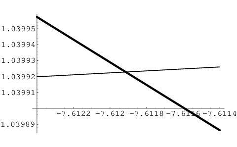
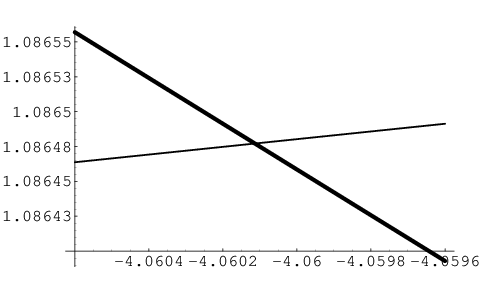
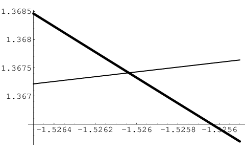
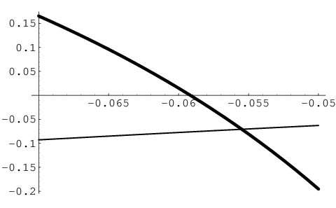
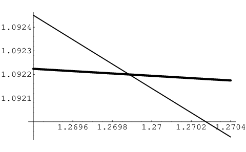
Now, in order to show the existence of a one-parameter family of weakly-complete CMC $1$ faces of genus $1$ with two ends which satisfy equality of the Osserman-type inequality, we find values $c\in\mathbb{R}\setminus\{0\}$ and $a>1$ so that $|f_{1}|=|f_{2}|>1$ and $f_{1}=f_{2}$ . By numerical experiments using Mathematica, we found such values (see Figure 3). Also, by Corollary A.4 in Appendix A, we see that the ends are elliptic ends for $c<0$ (resp. hyperbolic ends for $c>0$ ).

Refer to caption — Figure 3. The function $f_{1}$ (thin curve) and $f_{2}$ (thick curve) when $a=2$ . The horizontal axis represents $c$ , and the vertical axis represents $f_{1}$ and $f_{2}$ . We see that $f_{1}$ and $f_{2}$ intersect 6 times for $c\in(-9,4)$ , at $c\approx-7.6119$ , $c\approx-4.06015$ , $c\approx-1.526035$ , $c\approx-0.55$ , $c\approx 1.26988$ , and $f_{1}=f_{2}>1$ except for $c\approx-0.55$ .

Appendix A Criteria for the types of ends

Here we give the criteria for when an end of the genus $1$ catenoid given in (2.1) and (2.2) is elliptic or hyperbolic. First we give the following lemma:

Lemma A.1.

Let $f:M\to\mathbb{S}^{3}_{1}$ be a CMC $1$ face and $\gamma$ a loop in $M$ . Then the eigenvalues of the monodromy matrix with respect to $\gamma$ do not depend on the choice of the holomorphic null lift $F$ of $f$ .

Proof.

Let $(G,Q)$ be a Weierstrass data of $f$ and $F_{1},F_{2}:\widetilde{M}\to SL(2,\mathbb{C})$ solutions of Equation (1.2). Then there exists a constant $B\in SL(2,\mathbb{C})$ such that $F_{1}=F_{2}B$ . Let $\tau$ be the deck transformation of $\widetilde{M}$ associated to the homotopy class of $\gamma$ and $\Phi_{j}$ ( $j=1,2$ ) the monodromy matrix of $F_{j}$ with respect to $\gamma$ . Then

	$\displaystyle F_{1}\circ\tau$	$\displaystyle=F_{1}\Phi_{1}=F_{2}B\Phi_{1}$
		$\displaystyle=(F_{2}B)\circ\tau=F_{2}\Phi_{2}B.$

Thus $\Phi_{1}=B^{-1}\Phi_{2}B$ and hence the eigenvalues of $\Phi_{1}$ and $\Phi_{2}$ are the same, proving the lemma. ∎

So to determine the type of an end, we can take any holomorphic null lift $F$ of $f$ . Let $F=(F_{jk})_{j,k=1,2}:\widetilde{M}\to SL(2,\mathbb{C})$ be a holomorphic null lift of $f$ . Direct calculation shows that

(E.1)		$\displaystyle\frac{d^{2}F_{1j}}{dz^{2}}-\frac{1}{w}\frac{dw}{dz}\frac{dF_{1j}}{dz}+\frac{c}{w}\frac{dw}{dz}F_{1j}$	$\displaystyle=0,$
(E.2)		$\displaystyle\frac{d^{2}F_{2j}}{dz^{2}}+\frac{1}{w}\frac{dw}{dz}\frac{dF_{2j}}{dz}+\frac{c}{w}\frac{dw}{dz}F_{2j}$	$\displaystyle=0$

for $j=1,2$ . We consider the end $(z,w)=(\infty,1)$ . Let $\Delta^{*}\subset M$ be a neighborhood of $(z,w)=(\infty,1)$ . We set $\zeta=1/z$ . Without loss of generality we may assume $\Delta^{*}=\{\zeta\in\mathbb{C}\,|\,0<|\zeta|<1\}$ . We set $\Delta=\Delta^{*}\cup\{0\}$ . Then Equations (E.1) and (E.2) become

(A.1)		$\displaystyle\zeta^{2}\frac{d^{2}F_{1j}}{d\zeta^{2}}+\zeta p_{1}(\zeta)\frac{dF_{1j}}{dz}+q(\zeta)F_{1j}$	$\displaystyle=0,$
(A.2)		$\displaystyle\zeta^{2}\frac{d^{2}F_{2j}}{dz^{2}}+\zeta p_{2}(\zeta)\frac{dF_{2j}}{dz}+q(\zeta)F_{2j}$	$\displaystyle=0,$

where

p_{1}(\zeta)=2-\frac{1}{w}\frac{dw}{d\zeta}\zeta,\qquad p_{2}(\zeta)=2+\frac{1}{w}\frac{dw}{d\zeta}\zeta\qquad\text{and}\qquad q(\zeta)=-\frac{c}{w}\frac{dw}{d\zeta}.

Note that

\frac{1}{w}\frac{dw}{d\zeta}=\frac{(1-a)(a\zeta^{2}+1)}{(\zeta^{2}-1)(a^{2}\zeta^{2}-1)}=(1-a)+\mathcal{O}(\zeta^{2}).

Fundamental systems of solutions $\{X_{1},X_{2}\}$ of Equation (A.1) and $\{Y_{1},Y_{2}\}$ of Equation (A.2) can be chosen as

(A.3)		$\displaystyle X_{1}=\zeta^{(-1+m)/2}\xi_{1}(\zeta),\qquad$	$\displaystyle X_{2}=\zeta^{(-1-m)/2}\xi_{2}(\zeta)+k_{1}X_{1}\log\zeta,$
(A.4)		$\displaystyle Y_{1}=\zeta^{(-1+m)/2}\eta_{1}(\zeta),\qquad$	$\displaystyle Y_{2}=\zeta^{(-1-m)/2}\eta_{2}(\zeta)+k_{2}Y_{1}\log\zeta,$

where

m=\sqrt{1-4c(a-1)},

and $\xi_{j}$ and $\eta_{j}$ ( $j=1,2$ ) are holomorphic functions on $\Delta$ with $\xi_{j}(0)\neq 0$ and $\eta_{j}(0)\neq 0$ , and the constant $k_{1}$ (resp. $k_{2}$ ) is called the log-term coefficient of the solutions of Equation (A.1) (resp. (A.2)). See, for example, [RUY2, Appendix A].

Although $m$ can be either a positive real or is purely imaginary, here we only consider the case $m\not\in\mathbb{Z}$ . In this case, it is known that

k_{1}=k_{2}=0.

Moreover, we have the following lemma:

Lemma A.2.

There exists a matrix $\Lambda\in SL(2,\mathbb{C})$ such that

(A.5)

F\Lambda=\begin{pmatrix}\zeta^{(-1+m)/2}A(\zeta)&\zeta^{(-1-m)/2}B(\zeta)\\ \zeta^{(-1+m)/2}C(\zeta)&\zeta^{(-1-m)/2}D(\zeta)\end{pmatrix},

where $A$ , $B$ , $C$ and $D$ are holomorphic functions on $\Delta$ such that $A(0)$ , $B(0)$ , $C(0)$ and $D(0)$ are all nonzero.

Proof.

Since $f$ is not totally umbilic, $F_{11}$ and $F_{12}$ are linearly independent and are linear combinations of the $X_{1}$ and $X_{2}$ in Equation (A.3). Then there exists a matrix $\Lambda\in SL(2,\mathbb{C})$ such that

F\Lambda=\begin{pmatrix}\zeta^{(-1+m)/2}A(\zeta)&\zeta^{(-1-m)/2}B(\zeta)\\ C_{1}\zeta^{(-1+m)/2}\eta_{1}(\zeta)+C_{2}\zeta^{(-1-m)/2}\eta_{2}(\zeta)&D_{1}\zeta^{(-1+m)/2}\eta_{1}(\zeta)+D_{2}\zeta^{(-1-m)/2}\eta_{2}(\zeta)\end{pmatrix},

where $C_{j}$ and $D_{j}$ ( $j=1,2$ ) are constants, and $A$ and $B$ are holomorphic functions on $\Delta$ such that $A(0)\neq 0$ and $B(0)\neq 0$ . Since $F\Lambda\in SL(2,\mathbb{C})$ , we have

	$\displaystyle 1$	$\displaystyle=\det(F\Lambda)$
		$\displaystyle=D_{1}A(\zeta)\eta_{1}(\zeta)\zeta^{-1+m}+\bigl(D_{2}A(\zeta)\eta_{2}(\zeta)-C_{1}B(\zeta)\eta_{1}(\zeta)\bigr)\zeta^{-1}-C_{2}B(\zeta)\eta_{2}(\zeta)\zeta^{-1-m}.$

Since $A(0)$ , $B(0)$ and $\eta_{j}(0)$ are all nonzero, it follows that $D_{1}=C_{2}=0$ . Setting $C(\zeta)=C_{1}\eta_{1}(\zeta)$ and $D(\zeta)=D_{2}\eta_{2}(\zeta)$ , and noting that $C(0)\neq 0$ and $D(0)\neq 0$ , we have the conclusion. ∎

Proposition A.3.

Let $M$ be the Riemann surface defined as in Equation (2.1) and $f:M\to\mathbb{S}^{3}_{1}$ the CMC $1$ face constructed from the Weierstrass data as in Equation (2.2). Then the monodromy of an end is elliptic (resp. hyperbolic) if $m\in\mathbb{R}^{+}\setminus\mathbb{N}$ (resp. $m\in i\mathbb{R}\setminus\{0\}$ ).

Proof.

By Lemma A.1, we can choose $F\Lambda$ as in Equation (A.5) as a holomorphic null lift of $f$ . Let $\gamma$ be a loop around an end and $\tau$ the deck transformation of $\widetilde{M}$ associated to the homotopy class of $\gamma$ . Then

(F\Lambda)\circ\tau=(F\Lambda)\begin{pmatrix}-e^{m\pi i}&0\\ 0&-e^{m\pi i}\end{pmatrix}=(F\Lambda)\Phi_{\gamma}.

Thus the eigenvalues of $\Phi_{\gamma}$ are $-e^{\pm m\pi i}$ , which are in $\mathbb{S}^{1}$ (resp. $\mathbb{R}\setminus\{1\}$ ) if $m\in\mathbb{R}^{+}\setminus\mathbb{N}$ (resp. $m\in i\mathbb{R}\setminus\{0\}$ ), proving the proposition. ∎

Corollary A.4.

If $a=2$ , then the monodromy of an end is elliptic (resp. hyperbolic) if $c<0$ (resp. $c>0$ ).

References

[AA] R. Aiyama and K. Akutagawa, Kenmotsu-Bryant type representation formulas for constant mean curvature surfaces in $\mathbb{H}^{3}(-c^{2})$ and $\mathbb{S}^{3}_{1}(c^{2})$ , Ann. Global Anal. Geom. (1) 17 (1998), 49–75.
[Ak] K. Akutagawa, On spacelike hypersurfaces with constant mean curvature in the de Sitter space, 196 (1987), 13–19.
[B] R. Bryant, Surfaces of Mean Curvature One in Hyperbolic Space, Astérisque 154-155 (1987), 321–347.
[FLS1] I. Fernandez, F. J. Lopez and R. Souam, The space of complete embedded maximal surfaces with isolated singularities in the 3-dimensional Lorentz-Minkowski space $\mathbb{L}^{3}$ , Math. Ann. 332 (2005), 605–643.
[FLS2] by same author, The moduli space of embedded singly periodic maximal surfaces with isolated singularities in the Lorentz-Minkowski space $\mathbb{L}^{3}$ , preprint, math.DG/0412190.
[F] S. Fujimori, Spacelike CMC $1$ surfaces with elliptic ends in de Sitter $3$ -Space, to appear in Hokkaido Math. J.
[FRUYY] S. Fujimori, W. Rossman, M. Umehara, K. Yamada and S.-D. Yang, Spacelike mean curvature one surfaces in de Sitter $3$ -space, in preparation.
[FSUY] S. Fujimori, K. Saji, M. Umehara and K. Yamada, Singularities of maximal surfaces, preprint, math.DG/0510366.
[KUY] M. Kokubu, M. Umehara and K. Yamada, An elementary proof of Small’s formula for null curves in ${\rm PSL}(2,\boldsymbol{C})$ and an analogue for Legendrian curves in ${\rm PSL}(2,\boldsymbol{C})$ , Osaka J. Math. 40 (2003), 697–715.
[KY] Y. W. Kim and S.-D. Yang, A family of maximal surfaces in Lorentz-Minkowski three-space, to appear in Proc. A.M.S.
[LY] S. Lee and S.-D. Yang, Spacelike constant mean curvature $-1$ trinoids in de Sitter three-space, to appear in Osaka J. Math.
[P] B. Palmer, Spacelike constant mean curvature surfaces in pseudo-Riemannian space forms, Ann. Global Anal. Geom. (3) 8 (1990), 217–226.
[R] J. Ramanathan, Complete spacelike hypersurfaces of constant mean curvature in de Sitter space, Indiana Univ. Math. J. (2) 36 (1987), 349–359.
[RS] W. Rossman and K. Sato, Constant mean curvature surfaces with two ends in hyperbolic space, Experiment. Math. 7 (1998), 101–119.
[RUY1] W. Rossman, M. Umehara and K. Yamada, Irreducible constant mean curvature $1$ surfaces in hyperbolic space with positive genus, Tohoku Math. J. 49 (1997), 449–484.
[RUY2] by same author, Meanean curvature $1$ surfaces in hyperbolic $3$ -space with low total curvature I, Hiroshima Math. J. 34 (2004), 21–56.
[S] A. J. Small, Surfaces of Constant Mean Curvature 1 in $H^{3}$ and Algebraic Curves on a Quadric, Proc. Amer. Math. Soc. 122 (1994), 1211–1220.
[UY1] M. Umehara and K. Yamada, Complete surfaces of constant mean curvature $1$ in the hyperbolic $3$ -space, Ann. of Math. (2) 137 (1993), 611–638.
[UY2] by same author, A duality on CMC- $1$ surfaces in hyperbolic space, and a hyperbolic analogue of the Osserman inequality, Tsukuba J. Math. (1) 21 (1997), 229–237.
[UY3] by same author, Maximal surfaces with singularities in Minkowski space, to appear in Hokkaido Math. J.

Spacelike mean curvature 11 surfaces of genus 11 with two ends in de Sitter 33-SpaceThanks: 2000 Mathematics Subject Classification. 53A10, 53B30. Key words and phrases. de Sitter 33-space, spacelike CMC 11 surface, genus 11 surface.

Abstract.

Introduction

1. Preliminaries

1.1. de Sitter 33-space

1.2. CMC 11 faces

Definition 1.1.

Theorem 1.2.

Remark 1.3.

1.3. Closing conditions for CMC 11 faces

Definition 1.4.

Remark 1.5.

Definition 1.6.

Remark 1.7.

Definition 1.8.

Remark 1.9.

1.4. Osserman-type inequality

Theorem 1.10 (Osserman-type inequality [F]).

1.5. The hollow ball model

2. CMC 11 faces of genus 11

Lemma 2.1 ([RS, Lemmas 5.1 and 5.2]).

Lemma 2.2.

Proof.

Lemma 2.3.

Lemma 2.4.

Proof.

Lemma 2.5.

Remark 2.6.

Theorem 2.7.

Proof.

Lemma 2.8.

Proof.

Example 2.9.

Appendix A Criteria for the types of ends

Lemma A.1.

Proof.

Lemma A.2.

Proof.

Proposition A.3.

Proof.

Corollary A.4.

References

Spacelike mean curvature $1$ surfaces of genus $1$
with two ends in de Sitter $3$ -SpaceThanks: 2000 Mathematics Subject Classification. 53A10, 53B30.
Key words and phrases. de Sitter $3$ -space, spacelike CMC $1$ surface, genus $1$ surface.

1.1. de Sitter $3$ -space

1.2. CMC $1$ faces

1.3. Closing conditions for CMC $1$ faces

2. CMC $1$ faces of genus $1$