跳到论文正文
W Papers独立论文阅读器 arXiv:math/0605337 论文正文 计算阅读时间 · 0%
引用这篇论文根据当前论文元数据生成,正式投稿前建议核对。


License: Assumed arXiv.org perpetual non-exclusive license
arXiv:math/0605337v3 [math.PR] 24 Apr 2008

Contour lines of the
two-dimensional discrete Gaussian free field

Oded Schramm    Scott Sheffield
Abstract

We prove that the chordal contour lines of the discrete Gaussian free field converge to forms of SLE(4)(4). Specifically, there is a constant λ>0\lambda>0 such that when hh is an interpolation of the discrete Gaussian free field on a Jordan domain — with boundary values −λ-\lambda on one boundary arc and λ\lambda on the complementary arc — the zero level line of hh joining the endpoints of these arcs converges to SLE(4)(4) as the domain grows larger. If instead the boundary values are −a<0-a<0 on the first arc and b>0b>0 on the complementary arc, then the convergence is to SLE(4,a/λ−1,b/λ−1)(4;a/\lambda-1,b/\lambda-1), a variant of SLE(4)(4).

1 Introduction

1.1 Main result

The two-dimensional massless Gaussian free field (GFF) is a two-dimensional-time analog of Brownian motion. Just as Brownian motion is a scaling limit of simple random walks and various other one-dimensional systems, the GFF is a scaling limit of several discrete models for random surfaces. Among these is the discrete Gaussian free field (DGFF), also called the harmonic crystal. We presently discuss the basic definitions and describe the main results of the current work, postponing an overview of the history and general context to Section 1.3.

Let G=(V,E)G=(V,E) be a finite graph and let V∂⊂VV_{\partial}\subset V be some nonempty set of vertices. Let Ω\Omega be the set of functions h:V→ℝh:V\to\mathbb{R} that are zero on V∂V_{\partial}. Clearly, Ω\Omega may be identified with ℝV∖V∂\mathbb{R}^{V\smallsetminus V_{\partial}}. The DGFF on GG with zero boundary values on V∂V_{\partial} is the probability measure on Ω\Omega whose density with respect to Lebesgue measure on ℝV∖V∂\mathbb{R}^{V\smallsetminus V_{\partial}} is proportional to

exp(∑{u,v}∈E−12(h(v)−h(u))2).\exp\Bigl(\sum_{\{u,v\}\in E}-\frac{1}{2}\,\bigl(h(v)-h(u)\bigr)^{2}\Bigr). (1.1)

Note that under the DGFF measure, hh is a multi-dimensional Gaussian random variable. Moreover, the DGFF is a rather natural discrete model for a random field: the term −(h(v)−h(u))2/2-(h(v)-h(u))^{2}/2 corresponding to each edge {u,v}\{u,v\} penalizes functions hh which have a large gradient along the edge.

Now fix some function h∂:V∂→ℝh_{\partial}:V_{\partial}\to\mathbb{R}, and let Ωh∂\Omega_{h_{\partial}} denote the set of functions h:V→ℝh:V\to\mathbb{R} that agree with h∂h_{\partial} on V∂V_{\partial}. The probability measure on Ωh∂\Omega_{h_{\partial}} whose density with respect to Lebesgue measure on ℝV∖V∂\mathbb{R}^{V\smallsetminus V_{\partial}} is proportional to (1.1) is the DGFF with boundary values given by h∂h_{\partial}.

Let T​GTG be the usual triangular grid in the complex plane, i.e., the graph whose vertex set is the integer span of 11 and eπ​i/3=(1+3​i)/2e^{\pi\,i/3}=(1+\sqrt{3}\,i)/2, with straight edges joining vv and ww whenever |v−w|=1|v-w|=1. A T​GTG-domain D⊂ℝ2≅ℂD\subset\mathbb{R}^{2}\cong\mathbb{C} is a domain whose boundary is a simple closed curve comprised of edges and vertices in T​GTG. Let V=VD¯V=V_{\overline{D}} be the set of T​GTG-vertices in the closure of DD, let G=GDG=G_{D} be the induced subgraph of T​GTG with vertex set VD¯V_{\overline{D}}, and write V∂=∂D∩VD¯V_{\partial}=\partial D\cap V_{\overline{D}}. While introducing our main results, we will focus on graphs GDG_{D} and boundary sets V∂V_{\partial} of this form (though analogous results hold if we replace T​GTG with another doubly periodic planar graph; see Section 1.5).

We may assume that any function f:V→ℝf:V\rightarrow\mathbb{R} is interpolated to a continuous function on the closure of DD which is affine on each triangle of T​GTG. We often interpret ff as a surface embedded in three dimensions and refer to f⁡(v)f(v) as the height of the surface at vv.

Refer to caption

Refer to caption

Figure 1.1: (a) DGFF on 90×9090\times 90 hexagon array with boundary values λ\lambda on the right and −λ-\lambda on the left; faces shaded by height. (b) Surface plot of DGFF.

Let ∂D=∂+∪∂−{\partial}D={\partial}_{+}\cup{\partial}_{-} be a partition of the boundary of a T​GTG-domain DD into two disjoint arcs whose endpoints are midpoints of two distinct T​GTG-edges in ∂D{\partial}D. Fix two constants a,b>0a,b>0. Let hh be an instance of the DGFF on (GD,V∂)(G_{D},V_{\partial}), with boundary function h∂h_{\partial} equal to −a-a on the vertices in ∂−{\partial}_{-} and equal to bb on the vertices in ∂+{\partial}_{+}. Then hh (linearly interpolated on triangles) almost surely assumes the value zero on a unique piecewise linear path γh\gamma_{h} connecting the two boundary edges containing endpoints of ∂+{\partial}_{+}.

In Section 1.4, we will briefly review the definition of SLE⁡(4)\mathrm{SLE}(4) (a particular type of random chordal path connecting a pair of boundary points of DD whose randomness comes from a one-dimensional Brownian motion), along with the variants of SLE⁡(4)\mathrm{SLE}(4) denoted SLE⁡(4,ρ1,ρ2)\mathrm{SLE(4;\rho_{1},\rho_{2})}. Our main result, roughly stated, is the following:

Theorem 1.1.

Let DD be a T​GTG-domain, ∂D=∂+∪∂−{\partial}D={\partial}_{+}\cup{\partial}_{-} and let hh and γh\gamma_{h} be as above. There is a constant λ>0\lambda>0 such that if a=b=λa=b=\lambda, then as the triangular mesh gets finer, the random path γh\gamma_{h} converges in distribution to SLE⁡(4)\mathrm{SLE}(4). If a,b≥λa,b\geq\lambda are not assumed to equal λ\lambda, then the convergence is to SLE⁡(4,a/λ−1,b/λ−1)\mathrm{SLE(4;{a/\lambda-1},{b/\lambda-1})}.

See Section 1.5 for a more precise version, which describes the topology under which convergence is attained. As explained there, we can also prove convergence in a weaker form when the conditions a,b≥λa,b\geq\lambda are relaxed.

We will elaborate on the role of the constant λ\lambda in §1.2. This constant depends only on the lattice used. Although we do not prove it in this paper, for the triangular grid the value of λ\lambda is λT​G:=3−1/4π/8\lambda_{TG}:=3^{-1/4}\sqrt{\pi/8} (see Section 1.7).

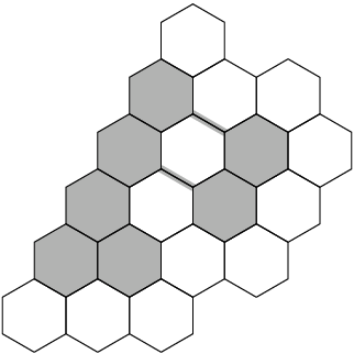
Figure 1.1 illustrates a dual perspective on an instance of γh\gamma_{h}. Here, each vertex in the closure of a rhombus-shaped T​GTG-domain DD is replaced with a hexagon in the honeycomb lattice. Call hexagons positive or negative according to the sign of hh. Then there is a cluster of positive hexagons that includes the positive boundary hexagons, a similar cluster of negative hexagons, and a path γ\gamma forming the boundary between these two clusters. Figure 1.1 depicts a computer generated instance of the DGFF—with ±λ\pm\lambda boundary conditions—and the corresponding γ\gamma. Followed from bottom to top, the interface γ\gamma turns right when it hits a negative hexagon, left when it hits a positive hexagon. It closely tracks the boundary-hitting zero contour line γh\gamma_{h} in the following sense: the edges in γ\gamma are the duals of the edges of T​GTG that are crossed by γh\gamma_{h}. This is because hh is almost surely non-zero at each vertex in VV, so whenever a zero contour line contains a point on an edge of T​GTG, hh must be positive on one endpoint of that edge and negative on the other; hence the dual of that edge separates a positive hexagon from a negative hexagon.

In the fine mesh limit, there will be no difference between γ\gamma and γh\gamma_{h}. Thus (by Theorem 1.1) the path in Figures 1.1.a and 1.2.a approximates SLE⁡(4)\mathrm{SLE}(4), while the path of Figure 1.3.a approximates SLE⁡(4,2,2)\mathrm{SLE(4;2,2)}. We will state and prove most of our results in terms of the dual perspective displayed in the figures.

1.2 Conditional expectation and the height gap

We derive the following well known facts as a warm-up in Section 2.1 (see also, e.g., [Gia02]):

Boundary influence: The law of the DGFF with boundary conditions h∂:V∂→ℝh_{\partial}:V_{\partial}\rightarrow\mathbb{R} is the same as that of the DGFF with boundary conditions 00 plus a deterministic function h~∂:V→ℝ\tilde{h}_{\partial}:V\rightarrow\mathbb{R} which is the unique discrete harmonic interpolation of h∂h_{\partial} to VV. (By discrete harmonic we mean that for each v∈V∖V∂v\in V\smallsetminus V_{\partial}, the value h⁡(v)h(v) is equal to the average value of h⁡(w)h(w) over ww adjacent to vv.) In particular, the expected value of h⁡(v)h(v) is discrete harmonic in V∖V∂V\smallsetminus V_{\partial}.

Markov property: Let h:V→ℝh:V\rightarrow\mathbb{R} be a random function whose law is the DGFF on GG with some boundary values h∂h_{\partial} on V∂V_{\partial}. Then given the values of hh on a superset V0⊃V∂V_{0}\supset V_{\partial}, the conditional law of hh is that of a DGFF on GG with boundary set V0V_{0} and with boundary values equal to the given values.

From these facts it follows that conditioned on the path γ\gamma described in the previous section and on the values of hh on the hexagons adjacent to γ\gamma, the expected value of hh is discrete harmonic in the remainder of GDG_{D}. Figures 1.2 and 1.3 illustrate the expected value of hh conditioned on the values of hh on the hexagons adjacent to γ\gamma.

The reader may observe in Figure 1.2 that although the expected value of hh given the values along γ\gamma varies a great deal among hexagons close to γ\gamma, the expected value at five or ten lattice spacings away from γ\gamma appears to be roughly constant along either side of γ\gamma. On the other hand in Figure 1.3, away from γ\gamma, the expected height appears to be a smooth but non-constant function. In a sense we make precise in Section 3 (see Theorem 3.28), the values −λ-\lambda and λ\lambda describe the expected value of hh, conditioned on γ\gamma, at the vertices near (but not microscopically near) the left and right sides of γ\gamma; in the fine mesh limit there is thus an “expected height gap” of 2​λ2\,\lambda between the two sides of γ\gamma. In Figure 1.2 the height expectation appears constant away from γ\gamma, because the boundary values of ±λ\pm\lambda are the same as the expected values near (but not microscopically near) γ\gamma.

Once we have established the height gap result, the proof of Theorem 1.1 (at least for the simplest case that the boundary conditions are −λ-\lambda and λ\lambda) is similar to the proof that the harmonic explorer converges to SLE⁡(4)\mathrm{SLE}(4), as given by the present authors in [SS05], which, in turn, follows the same strategy as the proof of convergence of the loop-erased random walk to SLE⁡(2)\mathrm{SLE}(2) and the uniform spanning tree Peano curve to SLE⁡(8)\mathrm{SLE}(8) in [LSW04].

Refer to caption

Refer to caption

Figure 1.2: (a) Expectation of DGFF with boundary values ±λ\pm\lambda given its values at hexagons bordering interface. (b) Surface plot of the above.

Refer to caption

Refer to caption

Figure 1.3: (a) Expectation of DGFF given its values at hexagons bordering interface; exterior boundary values are −3​λ-3\lambda on left, 3​λ3\lambda on right. (b) Surface plot of the above.

We will now briefly describe some of the key ideas in the proof of the height gap result. The main step is to show that if one samples a vertex zz on γ\gamma according to discrete harmonic measure viewed from a typical point far away from γ\gamma, then the absolute value of h⁡(z)h(z) is close to independent of the values of hh (and geometry of γ\gamma) at points that are not microscopically close to zz. In other words, if we start a random walk SS at a typical point in the interior of DD and stop the first time it hits a vertex zz which either belongs to V∂V_{\partial} or corresponds to a hexagon incident to γ\gamma, then (conditioned on z∉V∂z\not\in V_{\partial}), the random variable |h⁡(z)||h(z)| (and in particular its conditional expectation) is close to independent of the behavior of γ\gamma and hh at vertices far away from zz.

To prove this, we will actually prove something stronger, namely that (up to multiplication by −1-1) the collection of all of the values of hh (and the geometry of γ\gamma) in a microscopic neighborhood of zz is essentially independent of the values of hh (and the geometry of γ\gamma) at points that are not microscopically close to zz. One consequence of our analysis is Theorem 3.21, which states that if one takes zz to be the origin of a new coordinate system and conditions on the behavior of γ\gamma and SS outside of a ball of radius RR centered at zz and SS starts outside that ball, then as RR tends to infinity the conditional law of the interface γ\gamma has a weak limit (which is independent of the sequence of boundary conditions chosen), which is the law of a random infinite path γ\gamma on the honeycomb grid T​G∗TG^{*} (almost surely containing an edge adjacent to the hexagon centered at the origin z=0z=0). We will define a function of such infinite paths γ\gamma which (in a certain precise sense) describes the expected value of |h⁡(z)||h(z)| conditioned on γ\gamma; the value λ\lambda is the expectation of this function when γ\gamma is chosen according to the limiting measure described above.

We remark that many important problems in statistical physics involve classifying the measures that can arise as weak limits of Gibbs measures on finite systems. In such problems, showing the uniqueness of the limiting measure often involves proving that properties of a random system near the origin are approximately independent of the properties of the system far away from the origin. In our case, we need to prove that in some sense the behavior of the triple (h,γ,S)(h,\gamma,S) near the the origin (i.e., the first point SS hits γ\gamma) is close to independent of the behavior of (h,γ,S)(h,\gamma,S) far from the origin.

Very roughly speaking, our strategy will be to describe the joint law of (h,γ,S)(h,\gamma,S) near the origin and (h,γ,S)(h,\gamma,S) far from the origin by considering a different measure in which the two are independent and weighting it by the probability that the inside and outside configurations properly “hook up” with one another. To get a handle on these “hook up” probabilities, we will need to develop various techniques to control the probabilities (conditioned on the values of hh on certain sets) that certain zero height level lines hook up with one another, as well as the probabilities that these level lines avoid certain regions. We will also need bounds on the probability that there exist clusters of positive or negative hexagons crossing certain regions; these are roughly in the spirit of the Russo-Seymour-Welsh theorems for percolation, but the proofs are entirely different. All of the height gap related results are proved in Section 3.

1.3 GFF definition and background

To help put our DGFF theorems in context and provide further intuition, we now briefly recall the definition of the (continuum) GFF and mention some basic facts described, e.g., in [She07]. Let Hs​(D)H_{s}(D) be the set of smooth functions supported on compact subsets of a planar domain DD, and let H⁡(D)H(D) be its Hilbert space completion under the Dirichlet inner product (f,g)∇=∫D∇f⋅∇g​𝑑x(f,g)_{\nabla}=\int_{D}\nabla f\cdot\nabla g\;dx, where d​xdx refers to area measure. We define an instance of the Gaussian free field to be the formal sum

h=∑i=1∞αi​fi,h=\sum_{i=1}^{\infty}\alpha_{i}f_{i},

where αi\alpha_{i} are i.i.d. one-dimensional standard (unit variance, zero mean) Gaussians and the fif_{i} are an orthonormal basis for H⁡(D)H(D). Although the sum does not converge pointwise or in H⁡(D)H(D), it does converge in the space of distributions [She07]. In particular, the sum

(h,g)∇:=∑i=1∞αi​(fi,g)∇(h,g)_{\nabla}:=\sum_{i=1}^{\infty}\alpha_{i}\,\bigl(f_{i},g\bigr)_{\nabla}

is almost surely convergent for every g∈Hs​(D)g\in H_{s}(D).

It is worthwhile to take a moment to compare with the situation where DD is one dimensional. If DD were a bounded open interval in ℝ\mathbb{R}, then the partial sums of h=∑i=1∞αi​fih=\sum_{i=1}^{\infty}\alpha_{i}f_{i} would almost surely converge uniformly to a limit, whose law is that of the Brownian bridge, having the value zero at the interval’s endpoints. If DD were the interval (0,∞)(0,\infty), then the partial sums would converge (uniformly on compact sets) to a function whose law is that of ordinary Brownian motion BtB_{t}, indexed by t∈[0,∞)t\in[0,\infty), with B0=0B_{0}=0 [She07].

Let gg be a conformal (i.e., bijective analytic) map from DD to another planar domain D′D^{\prime}. When gg is a rotation, dilation, or translation, it is obvious that

∫D′∇(f1∘g−1)⋅∇(f2∘g−1)​𝑑x=∫D(∇f1⋅∇f2)​𝑑x.\int_{D^{\prime}}\nabla(f_{1}\circ g^{-1})\cdot\nabla(f_{2}\circ g^{-1})\,dx=\int_{D}(\nabla f_{1}\cdot\nabla f_{2})\,dx.

for any f1,f2∈Hs​(D)f_{1},f_{2}\in H_{s}(D), and an elementary change of variables calculation gives this equality for any conformal gg. Taking the completion to H⁡(D)H(D), we see that the Dirichlet inner product—and hence the two-dimensional GFF—is invariant under conformal transformations of DD.

Up to a constant, the DGFF on a T​GTG-domain DD can be realized as a projection of the GFF on DD onto the subspace of H⁡(D)H(D) consisting of functions which are continuous and are affine on each triangle of DD [She07]. Note that if ff is such a function, then

(f,f)∇=36​∑(|f⁡(j)−f⁡(i)|2+|f⁡(k)−f⁡(i)|2+|f⁡(k)−f⁡(j)|2),(f,f)_{\nabla}=\frac{\sqrt{3}}{6}\sum\bigl(|f(j)-f(i)|^{2}+|f(k)-f(i)|^{2}+|f(k)-f(j)|^{2}\bigr),

where the sum is over all triangles (i,j,k)(i,j,k) in VD¯V_{\overline{D}}. This is because the area of each triangle is 3/4\sqrt{3}/4 and the norm of the gradient squared in the triangle is

23​(|f⁡(j)−f⁡(i)|2+|f⁡(k)−f⁡(i)|2+|f⁡(k)−f⁡(j)|2).\frac{2}{3}\left(|f(j)-f(i)|^{2}+|f(k)-f(i)|^{2}+|f(k)-f(j)|^{2}\right).

Since each interior edge of DD is contained in two triangles, for such ff,

∥f∥∇2=3−1/2∑{i,j}∈EI|f(j)−f(i)|2+3−1/22∑{i,j}∈E∂|f(j)−f(i)|2,\|f\|^{2}_{\nabla}=3^{-1/2}\sum_{\{i,j\}\in E_{I}}|f(j)-f(i)|^{2}+\frac{3^{-1/2}}{2}\sum_{\{i,j\}\in E_{\partial}}|f(j)-f(i)|^{2}, (1.2)

where EIE_{I} and E∂E_{\partial} are the interior and boundary (undirected) edges of T​GTG in D¯\overline{D}. We will refer to the sum ∑EI|f⁡(j)−f⁡(i)|2\sum_{E_{I}}|f(j)-f(i)|^{2} as the discrete Dirichlet energy of ff. It is equivalent—up to the constant factor 3−1/23^{-1/2} and an additive term depending only on boundary values of ff—to the Dirichlet energy (f,f)∇(f,f)_{\nabla} of the piecewise affine interpolation of ff to DD.

The above analysis suggests a natural coupling between the GFF and a sequence of DGFF approximations to the GFF (obtained by taking finer mesh approximations of the same domain). The GFF can also be obtained as a scaling limit of other discrete random surface models (e.g., solid-on-solid, dimer-height-function, and ∇ϕ\nabla\phi-interface models) [Ken01, NS97, Spe97]. Its Laplacian is a scaling limit of some Coulomb gas models, which describe random electrostatic charge densities in two-dimensional domains [Fol01, FS81, Kos77, KT73, Spe97]. Physicists often use heuristic connections to the GFF to predict properties of two-dimensional statistical physics models that are not obviously random surfaces or Coulomb gases (e.g., Ising and Potts models, O⁡(n)O(n) loop models) [dN83, DFMS97, Dup89, Kad78, KN04, Nie82, Nie84]. As a model for the field theory of non-interacting massless bosons, the GFF is a starting point for many constructions in quantum field theory, conformal field theory, and string theory [BPZ84, DFMS97, Gaw99, GJ87].

Because of the conformal invariance of the GFF, physicists and mathematicians have hypothesized that discrete random surface models that are believed or known to converge to the Gaussian free field (e.g., the discrete Gaussian free field, the height function of the oriented O⁡(n)O(n) loop model with n=2n=2, height functions for domino and lozenge tilings) have level sets with conformally invariant scaling limits [Con89, DS87, DS88, SD87, KDH02, HK01, Ken01, KH95, KHS00, Nie82]. Our results confirm this hypothesis for the discrete Gaussian free field.

Various properties of the DGFF contour lines (such as winding exponents and the fact that the fractal dimension is 3/23/2) have been predicted correctly in the physics literature [Con89, DS88, DS87, SD87, HK01, KDH02, KH95, KHS00, Nie82]. The techniques used to make these predictions are also described in detail in the survey papers [Dup89, KN04, Nie84]. Analogous results about winding exponents and fractal dimension have now been proved rigorously for SLE\mathrm{SLE} [Sch00, RS05, Bef02].

The study of level lines of the DGFF and related random surfaces is also related to the study of equipotential lines of random charge distributions in statistical physics. The so-called two-dimensional Coulomb gas is a model for electrostatics in which the force between charged particles is inversely proportional to the distance between them. In this model, a continuous function f∈Hs​(D)f\in H_{s}(D) is the Coulomb gas electrostatic potential function (“grounded” at the boundary of DD) of −Δ​f-\Delta f, when Δ​f\Delta f is interpreted as a charge density function. The value (f,f)∇(f,f)_{\nabla} is then the total potential energy—also called the energy of assembly of the charge distribution −Δ​f-\Delta f. In the Coulomb gas model, this is the amount of energy required to move from a configuration in which the charge density is zero throughout DD to a configuration in which the charge density is given by −Δ​f-\Delta f.

In statistical physics, it is often natural to consider a probability distribution on configurations in which the probability of a configuration with potential energy HH is proportional to e−He^{-H}. If ρ\rho is a smooth charge distribution, then its energy of assembly is given by (−Δ−1​ρ,−Δ−1​ρ)∇=(ρ,−Δ−1​ρ)(-\Delta^{-1}\rho,-\Delta^{-1}\rho)_{\nabla}=(\rho,-\Delta^{-1}\rho); if we define ρ\rho to be the standard Gaussian in Δ​H​(D)\Delta H(D) determined by this quadratic form, then ρ\rho is the Laplacian of the Gaussian free field (which, like the GFF itself, is well defined as a random distribution but not as a function). In other words, the Laplacian of a Gaussian free field is a random distribution that we may interpret as a model for random charge density in a statistical physical Coulomb gas.

However, we stress that when physicists refer to the Coulomb gas method for O⁡(n)O(n) model computations, they typically have in mind a more complicated Coulomb gas model in which the charges are required to be discrete (i.e., ρ\rho is required to be a sum of unit positive and negative point masses) and hard core constraints may be enforced.

The surveys [BEMF86, Gia02, Spe97] contain additional references on lattice spin models that have the GFF as a scaling limit and Coulomb gas models that have its Laplacian as a scaling limit—for example, the harmonic crystal (a.k.a. the discrete Gaussian free field) with quadratic nearest-neighbor potential, the more general anharmonic crystal, the discrete-height Gaussian (where hh is a function on a lattice, with values restricted to integers), the Villain gas (where hh is a function on a lattice and the values of its discrete Laplacian 𝔭=−Δ​h{\mathfrak{p}}=-\Delta h are restricted to integers), and the hard core Coulomb gas (where hh is a function on a lattice and its discrete Laplacian 𝔭=−Δ​h{\mathfrak{p}}=-\Delta h is ±1\pm 1 valued).

The physics literature on applications of the GFF to field theory and statistical physics is large, and the authors themselves are only familiar with parts of it. Outside of these areas, there is a body of experimental and computational research on contour lines of random topographical surfaces, such as the surface of the earth. Mandelbrot’s famous How Long Is the Coast of Britain?… [Man67], which prefigured the notion of “fractal” introduced by Mandelbrot years later, is an early example. The results about contour lines in these studies (including fractal dimension computations) are less detailed than the ones provided here and are not all mathematically rigorous. However, some of the models are similar in spirit to the GFF, involving functions whose Fourier coefficients are independent Gaussians. An eclectic overview of this literature appears in [Isi92].

1.4 SLE\mathrm{SLE} background and prior convergence results

We now give a brief definition of (chordal) SLE⁡(κ)\mathrm{SLE}(\kappa) for κ>0\kappa>0. See also the surveys [Wer04, KN04, Law05, Car05] or [Law04]. The discussion below along with further discussion of the special properties of SLE⁡(4)\mathrm{SLE}(4) appears in another paper by the current authors [SS05]. That paper shows that SLE⁡(4)\mathrm{SLE}(4) is the scaling limit of a random interface called the harmonic explorer (designed in part to be a toy model for the DGFF contour line addressed here).

Let T>0T>0. Suppose that γ:[0,T]→ℍ¯\gamma:[0,T]\to\overline{\mathbb{H}} is a continuous simple path in the closed upper half plane ℍ¯\overline{\mathbb{H}} which satisfies γ⁡[0,T]∩ℝ={γ⁡(0)}={0}\gamma[0,T]\cap\mathbb{R}=\{\gamma(0)\}=\{0\}. For every t∈[0,T]t\in[0,T], there is a unique conformal homeomorphism gt:ℍ∖γ⁡[0,t]g_{t}:\mathbb{H}\smallsetminus\gamma[0,t] which satisfies the so-called hydrodynamic normalization at infinity

limz→∞gt​(z)−z=0.\lim_{z\to\infty}g_{t}(z)-z=0\,.

The limit

cap∞​(γ⁡[0,t]):=limz→∞z⁡(gt​(z)−z)/2\mathrm{cap}_{\infty}(\gamma[0,t]):=\lim_{z\to\infty}z(g_{t}(z)-z)/2

is real and monotone increasing in tt. It is called the (half plane) capacity of γ⁡[0,t]\gamma[0,t] from ∞\infty, or just capacity, for short. Since cap∞​(γ​[0,t])\mathrm{cap}_{\infty}(\gamma[0,t]) is also continuous in tt, it is natural to reparameterize γ\gamma so that cap∞​(γ⁡[0,t])=t\mathrm{cap}_{\infty}(\gamma[0,t])=t. Loewner’s theorem states that in this case the maps gtg_{t} satisfy his differential equation

∂tgt​(z)=2gt​(z)−Wt,g0​(z)=z,{\partial}_{t}g_{t}(z)=\frac{2}{g_{t}(z)-W_{t}}\,,\qquad g_{0}(z)=z\,, (1.3)

where Wt=gt​(γ⁡(t))W_{t}=g_{t}(\gamma(t)). (Since γ⁡(t)\gamma(t) is not in the domain of definition of gtg_{t}, the expression gt​(γ​(t))g_{t}(\gamma(t)) should be interpreted as a limit of gt​(z)g_{t}(z) as z→γ⁡(t)z\to\gamma(t) inside ℍ∖γ⁡[0,t]\mathbb{H}\smallsetminus\gamma[0,t]. This limit does exist.) The function t→Wtt\to W_{t} is continuous in tt, and is called the driving parameter for γ\gamma.

One may also try to reverse the above procedure. Consider the Loewner evolution defined by the ODE (1.3), where WtW_{t} is a continuous, real-valued function. For a fixed zz, the evolution defines gt​(z)g_{t}(z) as long as |gt​(z)−Wt||g_{t}(z)-W_{t}| is bounded away from zero. For z∈ℍ¯z\in\overline{\mathbb{H}} let τz\tau_{z} be the first time t≥0t\geq 0 in which gt​(z)g_{t}(z) and WtW_{t} collide, or set τz=∞\tau_{z}=\infty if they never collide. Then gt​(z)g_{t}(z) is well defined on {z∈ℍ¯:τz≥t}\{z\in\overline{\mathbb{H}}:\tau_{z}\geq t\}. The set Kt:={z∈ℍ¯:τz≤t}K_{t}:=\{z\in\overline{\mathbb{H}}:\tau_{z}\leq t\} is sometimes called the evolving hull of the evolution. In the case discussed above where the evolution is generated by a simple path γ\gamma parameterized by capacity and satisfying γ⁡(t)∈ℍ\gamma(t)\in\mathbb{H} for t>0t>0, we have Kt=γ⁡[0,t]K_{t}=\gamma[0,t].

The path of the evolution is defined as γ⁡(t)=limz→Wtgt−1​(z)\gamma(t)=\lim_{z\to W_{t}}g_{t}^{-1}(z), where zz tends to WtW_{t} from within the upper half plane ℍ\mathbb{H}, provided that the limit exists and is continuous. However, this is not always the case. The process (chordal) SLE⁡(κ)\mathrm{SLE}(\kappa) in the upper half plane, beginning at 00 and ending at ∞\infty, is the path γ⁡(t)\gamma(t) when WtW_{t} is κ​Bt\sqrt{\kappa}\,B_{t}, where Bt=B⁡(t)B_{t}=B(t) is a standard one-dimensional Brownian motion. (“Standard” means B⁡(0)=0B(0)=0 and 𝐄⁡[B​(t)2]=t{\bf E}[B(t)^{2}]=t, t≥0t\geq 0. Since (kBt:t≥0)(\sqrt{k}\,B_{t}:t\geq 0) has the same distribution as (Bκ​t:t≥0)(B_{\kappa\,t}:t\geq 0), taking Wt=Bκ​tW_{t}=B_{\kappa\,t} is equivalent.) In this case a.s. γ⁡(t)\gamma(t) does exist and is a continuous path. See [RS05] (κ≠8\kappa\neq 8) and [LSW04] (κ=8\kappa=8).

We now define the processes SLE⁡(κ,ρ1,ρ2)\mathrm{SLE(\kappa;\rho_{1},\rho_{2})}. Given a Loewner evolution defined by a continuous WtW_{t}, we will let xtx_{t} and yty_{t} be defined by xt:=sup{gt(x):x<0,x∉Kt}x_{t}:=\sup\{g_{t}(x):x<0,x\notin K_{t}\} and yt:=inf{gt(x):x>0,x∉Kt}y_{t}:=\inf\{g_{t}(x):x>0,x\notin K_{t}\}. When the Loewner evolution is generated by a simple path γ⁡(t)\gamma(t) satisfying γ⁡(t)∈ℍ\gamma(t)\in\mathbb{H} for t>0t>0, these points xtx_{t} and yty_{t} can be thought of as the two images of 00 under gtg_{t}. Note that by (1.3)

∂txt=2/(xt−Wt),∂tyt=2/(yt−Wt),{\partial}_{t}x_{t}=2/(x_{t}-W_{t}),\qquad{\partial}_{t}y_{t}=2/(y_{t}-W_{t})\,, (1.4)

for all tt such that xt<Wt<ytx_{t}<W_{t}<y_{t}. Beginning from an initial time rr for which xr<Wr<yrx_{r}<W_{r}<y_{r}, we define SLE⁡(κ,ρ1,ρ2)\mathrm{SLE(\kappa;\rho_{1},\rho_{2})} to be the evolution that makes (xt,Wt,yt)(x_{t},W_{t},y_{t}) a solution to the SDE system

d​Wt=κ​d​Bt+ρ1​d​tWt−xt+ρ2​d​tWt−yt,d​xt=2​d​txt−Wt,d​yt=2​d​tyt−Wt,dW_{t}=\sqrt{\kappa}\,dB_{t}+\frac{\rho_{1}\,dt}{W_{t}-x_{t}}+\frac{\rho_{2}\,dt}{W_{t}-y_{t}},\,\,\,dx_{t}=\frac{2\,dt}{x_{t}-W_{t}},\,\,\,dy_{t}\,=\,\frac{2\,dt}{y_{t}-W_{t}}, (1.5)

noting that existence and uniqueness of solutions to this SDE (at least from the initial time rr until the first s>rs>r for which either xs=Wsx_{s}=W_{s} or Ws=ysW_{s}=y_{s}) follow easily from standard results in [RY99]. (The xtx_{t} and yty_{t} are called force points because they apply a “force” affecting the drift of the process WtW_{t} by an amount inversely proportional to their distance from WtW_{t}.)

Some subtlety is involved in extending the definition of SLE⁡(κ,ρ1,ρ2)\mathrm{SLE(\kappa;\rho_{1},\rho_{2})} beyond times when WtW_{t} hits the force points, and in starting the process from the natural initial values x0=W0=y0=0x_{0}=W_{0}=y_{0}=0. This is closely related to the issues which come up when defining the Bessel processes of dimension less than two and will be discussed in more detail in Section 4.

Although many random self-avoiding lattice paths from the statistical physics literature are conjectured to have forms of SLE\mathrm{SLE} as scaling limits, rigorous proofs have thus far appeared only for a few cases: site percolation cluster boundaries on the hexagonal lattice (SLE⁡(6)\mathrm{SLE}(6), [Smi01]; see also [CN06]), branches (loop-erased random walk) and outer boundaries (random Peano curves) of uniform spanning tree (forms of SLE⁡(2)\mathrm{SLE}(2) and SLE⁡(8)\mathrm{SLE}(8) respectively, [LSW04]), the harmonic explorer (SLE⁡(4)\mathrm{SLE}(4), [SS05]), and boundaries of simple random walks (forms of SLE⁡(8/3)\mathrm{SLE}(8/3), [LSW03]).

In the latter case, conformal invariance properties follow almost immediately from the conformal invariance of two dimensional Brownian motion. In each of the other cases listed above, the initial step of the proof is to show that a certain function of the partially generated paths γ⁡([0,t])\gamma([0,t]), which is a martingale in tt when γ\gamma is SLE⁡(κ)\mathrm{SLE}(\kappa) for the appropriate κ\kappa, has a discrete analog which is (approximately or exactly) a martingale for the discrete paths and is approximately equivalent to the continuous version in the fine mesh limit. For loop-erased random walk, harmonic explorer, and uniform spanning tree Peano curves, this initial step is the easy part of the argument; it follows almost immediately from the fact that simple random walk converges to Brownian motion. The analogous step for site percolation on the hexagonal lattice, as given by [Smi01], is an ingenious but nonetheless short and simple argument.

By contrast, the analogous step in this paper (which requires the proof of the height gap lemma, as given in Section 3) is quite involved; it is the most technically challenging part of the current work and includes many new techniques and lemmas about the geometry of DGFF contours that we hope are interesting for their own sake.

Another way in which the DGFF differs from percolation, the harmonic explorer, and the uniform spanning tree is that it has a natural continuum analog (the GFF) which can be easily rigorously constructed without any reference to SLE\mathrm{SLE}, and which is itself (like Brownian motion) an object of great significance. It becomes natural to ask whether the DGFF results enable us to define the “contour lines” of the continuum GFF in a canonical way; we plan to answer this question (affirmatively) in a subsequent work (see Section 1.7).

A final difference is that, for the DGFF, there is a continuum of choices for left and right boundary conditions (aa and bb) which are equally natural a priori, so we are led to consider a family of paths SLE⁡(4,a/λ−1,b/λ−1)\mathrm{SLE(4;{a/\lambda-1},{b/\lambda-1})} instead of simply SLE⁡(4)\mathrm{SLE}(4). (The case a=b=0a=b=0 is particularly natural; see Figure 1.4.) In these processes, the driving parameters WtW_{t} are generally no longer Brownian motions (rather, they are continuous semimartingales with constant quadratic variation and a drift term that can become singular on a fractal set). Proving driving parameter convergence to these processes requires some rather general convergence infrastructure (Section 4.4), which we hope will be useful in other settings as well.

1.5 Precise statement of main result

Let ℍ\mathbb{H} be the upper half plane. Let DD be any T​GTG-domain and let ∂D=∂+∪∂−{\partial}D={\partial}_{+}\cup{\partial}_{-} be a partition of the boundary of DD into two disjoint arcs whose endpoints are midpoints of two T​GTG-edges contained in ∂D{\partial}D. As before, let VV denote the vertices of T​GTG in D¯\overline{D}. Let h∂=−ah_{\partial}=-a on ∂−∩V{\partial}_{-}\cap V and h∂=bh_{\partial}=b on ∂+∩V{\partial}_{+}\cap V, where aa and bb are positive constants.

Let h:V→ℝh:V\to\mathbb{R} be an instance of the DGFF with boundary conditions h∂h_{\partial}. Let ϕD\phi_{D} be any conformal map from DD to ℍ\mathbb{H} that maps ∂+{\partial}_{+} bijectively onto the positive real ray (0,∞)(0,\infty). (Note that ϕD\phi_{D} is unique up to positive scaling.)

There is almost surely a unique interface γ⊂D¯\gamma\subset\overline{D} between hexagons in the dual grid T​G∗TG^{*} containing T​GTG-vertices where hh is positive and such hexagons where hh is negative such that the endpoints of γ\gamma are on ∂D{\partial}D. In fact, the endpoints of γ\gamma are the same as the endpoints of ∂+{\partial}_{+}. (As mentioned above, this interface γ\gamma stays within a bounded distance from the zero height contour line γD\gamma_{D} of the affine interpolation of hh.) Now, ϕD∘γ\phi_{D}\circ\gamma is a random path on ℍ\mathbb{H} connecting 00 to ∞\infty. We will show that this path converges to a form of SLE⁡(4)\mathrm{SLE}(4). Rather than considering a fixed domain D^\hat{D} and a sequence of discrete domains DnD_{n} approximating D^\hat{D}, with the mesh tending to 00, we will employ a setup that is more general in which the mesh is fixed (the triangular lattice will not be rescaled), and we consider domains DD that become “larger”. The correct sense of “large” is measured by

rD=rD,ϕ:=radϕD−1​(i)​(D),{r_{D}}=r_{D,\phi}:=\mathrm{rad}_{\phi_{D}^{-1}(i)}(D)\,,

where radx​(D)\mathrm{rad}_{x}(D) denotes the radius of DD viewed from xx, i.e., infy∉D|x−y|\inf_{y\not\in D}|x-y|. Of course, if ϕD−1​(i)\phi_{D}^{-1}(i) is at bounded distance from ∂D{\partial}D, then the image of the triangular grid under ϕD\phi_{D} is not fine near ii, and there is no hope for approximating SLE\mathrm{SLE} by ϕD∘γ\phi_{D}\circ\gamma.

We have chosen to use ℍ\mathbb{H} as our canonical domain (mapping all other paths into ℍ\mathbb{H}), because it is the most convenient domain in which to define chordal SLE\mathrm{SLE}. However, to make the completion of ℍ\mathbb{H} a compact metric space, we will endow ℍ\mathbb{H} with the metric it inherits from its conformal map onto the unit disc 𝕌\mathbb{U}. Namely, we let d∗​(⋅,⋅)d_{*}(\cdot,\cdot) be the metric on ℍ¯∪{∞}\overline{\mathbb{H}}\cup\{\infty\} given by d∗​(z,w)=|Ψ⁡(z)−Ψ⁡(w)|d_{*}(z,w)=|\Psi(z)-\Psi(w)|, where Ψ⁡(z):=(z−i)/(z+i)\Psi(z):=(z-i)/(z+i) maps ℍ¯∪{∞}\overline{\mathbb{H}}\cup\{\infty\} onto 𝕌¯\overline{\mathbb{U}}. If z∈ℍ¯z\in\overline{\mathbb{H}}, then d∗​(zn,z)→0d_{*}(z_{n},z)\to 0 is equivalent to |zn−z|→0|z_{n}-z|\to 0, and d∗​(zn,∞)→0d_{*}(z_{n},\infty)\to 0 is equivalent to |zn|→∞|z_{n}|\to\infty.

If γ1\gamma_{1} and γ2\gamma_{2} are distinct unparametrized simple paths in ℍ¯\overline{\mathbb{H}}, then we define d𝒰​(γ1,γ2){d}_{\mathcal{U}}(\gamma_{1},\gamma_{2}) to be the infimum over all pairs (η1,η2)(\eta_{1},\eta_{2}) of parameterizations of γ1\gamma_{1} and γ2\gamma_{2} in [0,1][0,1] (i.e., ηj:[0,1]→ℍ¯\eta_{j}:[0,1]\to\overline{\mathbb{H}} is a simple path satisfying ηj​([0,1])=γj\eta_{j}([0,1])=\gamma_{j} for j=1,2j=1,2) of the uniform distance sup{d∗​(η1​(t),η2​(t)):t∈[0,1]}\sup\bigl\{d_{*}\bigl(\eta_{1}(t),\eta_{2}(t)\bigr):t\in[0,1]\bigr\} with respect to the metric d∗d_{*}.

Our strongest result is in the case where a,b≥λa,b\geq\lambda. We prove the following:

Theorem 1.2.

There is a constant λ>0\lambda>0 such that if a,b≥λa,b\geq\lambda, then as rD→∞{r_{D}}\to\infty, the random paths ϕD∘γ\phi_{D}\circ\gamma described above converge in distribution to SLE⁡(4,a/λ−1,b/λ−1)\mathrm{SLE(4;{a/\lambda-1},{b/\lambda-1})} with respect to the metric d𝒰{d}_{\mathcal{U}}.

In other words, for every ϵ>0\epsilon>0 there is some R=R⁡(ϵ)R=R(\epsilon) such that if rD>R{r_{D}}>R, then there is a coupling of ϕD∘γ\phi_{D}\circ\gamma and a path γSLE\gamma_{\mathrm{SLE}} whose law is that of SLE⁡(4,a/λ−1,b/λ−1)\mathrm{SLE(4;{a/\lambda-1},{b/\lambda-1})} such that

𝐏[d𝒰(ϕD∘γ,γSLE)>ϵ]<ϵ.{{\bf P}\Bigl[{d}_{\mathcal{U}}(\phi_{D}\circ\gamma,\gamma_{\mathrm{SLE}})>\epsilon\Bigr]}<\epsilon\,.

We first comment that it follows that when rDr_{D} is large, γ\gamma is “close” to ϕD−1∘γSLE\phi_{D}^{-1}\circ\gamma_{\mathrm{SLE}}. For example, if rD→∞r_{D}\to\infty and rD−1​Dr_{D}^{-1}\,D tends to a bounded domain D^\hat{D} whose boundary is a simple closed path in such a way that the boundaries of the domains may be parameterized to give uniform convergence of parameterized paths and if rD−1∂+r_{D}^{-1}{\partial}_{+} converges, then rD−1​γr_{D}^{-1}\,\gamma converges in law to the corresponding SLE in D^\hat{D}. To prove this from Theorem 1.2, we only need to note that in this case the maps rD−1​ϕD−1r_{D}^{-1}\phi_{D}^{-1} converge uniformly in ℍ¯∪{∞}\overline{\mathbb{H}}\cup\{\infty\} (see, e.g., [Pom92, Proposition 2.3]).

When we relax the assumption a,b≥λa,b\geq\lambda to a,b>0a,b>0, we still prove some sort of convergence to SLE⁡(4,a/λ−1,b/λ−1)\mathrm{SLE(4;{a/\lambda-1},{b/\lambda-1})}, but with respect to a weaker topology. In fact, we can allow aa and bb to be zero or even slightly negative, but in this case we need to appropriately adjust the above definition of the interface γ\gamma. Say that a hexagon in the hexagonal grid T​G∗TG^{*} dual to T​GTG is positive if either the center vv of the hexagon is in DD and h⁡(v)>0h(v)>0, or v∈∂+v\in{\partial}_{+}. Likewise, say that the hexagon is negative if v∈Dv\in D and h⁡(v)<0h(v)<0, or v∈∂−v\in{\partial}_{-}. Let γ\gamma be the unique oriented path in T​G∗TG^{*} that joins the two endpoints of ∂+{\partial}_{+}, has only positive hexagons adjacent to its right hand side and only negative hexagons adjacent to its left hand side. (If a,b>0a,b>0, this definition clearly agrees with the previous definition of γ\gamma.) We prove:

Theorem 1.3.

For every constant Λ¯>0\bar{\Lambda}>0 there is a constant Λ0=Λ0​(Λ¯)>0\Lambda_{0}=\Lambda_{0}(\bar{\Lambda})>0 such that if a,b∈[−Λ0,Λ¯]a,b\in[-\Lambda_{0},\bar{\Lambda}] and γ\gamma is the DGFF interface defined above, then as rD→∞r_{D}\to\infty the Loewner driving term W^t\hat{W}_{t} of ϕD∘γ\phi_{D}\circ\gamma parameterized by capacity from ∞\infty converges in law to the driving term WtW_{t} of SLE⁡(4,a/λ−1,b/λ−1)\mathrm{SLE(4;{a/\lambda-1},{b/\lambda-1})} with respect to the topology of locally uniform convergence. That is, for every T,ϵ>0T,\epsilon>0 there is some R>0R>0 such that if rD>Rr_{D}>R, then γ\gamma and SLE⁡(4,a/λ−1,b/λ−1)\mathrm{SLE(4;{a/\lambda-1},{b/\lambda-1})} may be coupled so that with probability at least 1−ϵ1-\epsilon

sup{|W^t−Wt|:t∈[0,T]}<ϵ.\sup\bigl\{|\hat{W}_{t}-W_{t}|:t\in[0,T]\bigr\}<\epsilon\,.

Some (essentially well-known) geometric consequences of this kind of convergence are proved in §4.7.

Figure 1.4: Zero height interfaces starting and ending on the boundary, shown for the discrete GFF on a 150×150150\times 150 hexagonal array with zero boundary. Interior white hexagons have height greater than 00; interior black hexagons have height less than 00; boundary hexagons (of height zero) are black. Hexagons that are not incident to a zero height interface that reaches the boundary are gray.

A particularly interesting case of Theorem 1.3 is the case a=0a=0 and b=0b=0, corresponding to the DGFF with zero boundary values. In this case, when hh is interpolated linearly to triangles, its zero level set will almost surely include a finite number of piecewise linear arcs in DD whose endpoints on ∂D\partial D are vertices of T​GTG. A dual representation of this set of arcs is shown in Figure 1.4. For any fixed choice of endpoints on the boundary, the interface connecting those endpoints will converge to SLE⁡(4,−1,−1)\mathrm{SLE(4;-1,-1)}. The limit of the complete set of arcs in Figure 1.4 is in some sense a coupling of SLE⁡(4,−1,−1)\mathrm{SLE(4;-1,-1)} processes, one for each pair of boundary points.

Finally, we discuss the generalizations: replace T​GTG with an arbitrary weighted doubly periodic planar lattice—i.e., a connected planar graph 𝔊⊂ℝ2\mathfrak{G}\subset\mathbb{R}^{2} invariant under two linearly independent translations, T1,T2T_{1},T_{2}, such that every compact subset of ℝ2\mathbb{R}^{2} meets only finitely many vertices and edges, together with a map ww from the edges of 𝔊\mathfrak{G} to the positive reals, which is invariant under T1T_{1} and T2T_{2}.

A 𝔊\mathfrak{G}-domain D⊂ℝ2D\subset\mathbb{R}^{2} is a domain whose boundary is a simple closed curve comprised of edges and vertices in 𝔊\mathfrak{G}. Let V=VD¯V=V_{\overline{D}} be the set of 𝔊\mathfrak{G}-vertices in the closure of DD, let G=GD=(V,E)G=G_{D}=(V,E) be the induced subgraph of 𝔊\mathfrak{G} with vertex set VD¯V_{\overline{D}}, and write V∂=∂D∩VD¯V_{\partial}=\partial D\cap V_{\overline{D}}. Given a boundary value function h∂:V∂→ℝh_{\partial}:V_{\partial}\to\mathbb{R}, the edge weighted DGFF on GG has a density with respect to Lebesgue measure on ℝV∖V∂\mathbb{R}^{V\smallsetminus V_{\partial}} which is proportional to

exp(∑{u,v}∈E−12w({u,v})(h(v)−h(u))2).\exp\Bigl(\sum_{\{u,v\}\in E}-\frac{1}{2}\,w\bigl(\{u,v\}\bigr)\bigl(h(v)-h(u)\bigr)^{2}\Bigr).

If every face of 𝔊\mathfrak{G} has three edges, then every vertex in the dual graph is an endpoint of exactly three edges, and the boundary between positive and negative faces can be defined as a simple path in this dual lattice, similar to the one shown in Figures 1.1.a. If not every face of 𝔊\mathfrak{G} has three edges, then we may “triangulate” 𝔊\mathfrak{G} by adding additional edges to 𝔊\mathfrak{G}, while maintaining the invariance under T1T_{1} and T2T_{2}, to make this the case (and set ww to zero on these edges so that their presence does not affect the law of the DGFF).

We define the weighted random walk on 𝔊\mathfrak{G} to be the Markov chain with transition probability w⁡({u,v})/∑v′w⁡({u,v′})w(\{u,v\})/\sum_{v^{\prime}}w(\{u,v^{\prime}\}) from uu to vv, where we take w⁡({u,v})=0w(\{u,v\})=0 unless uu and vv are neighbors in 𝔊\mathfrak{G}. It is well known and easy to prove that such a walk on the re-scaled lattice ϵ​𝔊\epsilon\mathfrak{G} converges to a linear transformation of time-scaled two-dimensional Brownian motion when ϵ\epsilon tends to zero (but since we could not find a reference, we very briefly explain this in §5). It is convenient to replace the embedding of 𝔊\mathfrak{G} into ℝ2\mathbb{R}^{2} described above with a linear transformation of that embedding that causes this limit to be standard Brownian motion.

Theorem 1.4.

Both Theorem 1.3 and Theorem 1.2 continue to hold if T​GTG is replaced by a general weighted doubly periodic planar lattice 𝔊\mathfrak{G}, as described above, provided that 𝔊\mathfrak{G} is embedded in ℝ2\mathbb{R}^{2} in such a way that the weighted random walk converges to Brownian motion.

If 𝔊\mathfrak{G} is the grid ℤ2\mathbb{Z}^{2}, then one natural way to triangulate 𝔊\mathfrak{G} is to add all the edges of the form {(x,y),(x+1,y+1)}\{(x,y),(x+1,y+1)\}. Another would be to add edges of the form {(x,y),(x+1,y−1)}\{(x,y),(x+1,y-1)\}. The above theorem implies, perhaps surprisingly, that the limiting law of the zero height interface is the same in either case, with no need for a linear change of coordinates.

1.6 Outline

Section 2 introduces the basic notation and assumptions that are necessary for the height gap results proved in Section 3. Sections 3.1, 3.2, 3.3, and 3.4 develop bounds and estimates related to the geometry of zero height interfaces. The random walk SS comes into the picture in Section 3.5, where we develop results about the near-independence of the triple (h,γ,S)(h,\gamma,S) on microscopic and macroscopic scales. Section 3.6 applies these results to prove uniqueness of the limiting measure, namely Theorem 3.21, and Section 3.7 applies this to prove our main height gap result, Theorem 3.28.

Based on Theorem 3.28, the convergence in the case where the boundary values are ±λ\pm\lambda is not too hard, using the method from [LSW04]. However, to prove the convergence to SLE⁡(4,a/λ−1,b/λ−1)\mathrm{SLE(4;{a/\lambda-1},{b/\lambda-1})} in Section 4, we need to contend with a few other issues which stem from the fact that the driving parameter of SLE⁡(4,a/λ−1,b/λ−1)\mathrm{SLE(4;{a/\lambda-1},{b/\lambda-1})} is the solution to an SDE with a drift term that blows up to infinity on a fractal set of times. To overcome these difficulties, we change coordinates to a coordinate system in which the drift terms stay bounded. In §4.4 we define and study approximate diffusions. These are random processes that are not necessarily Markov, but satisfy an approximate discrete version of an SDE. The Loewner driving term of the DGFF interface (before going to the scaling limit) is the approximate diffusion we are interested in. The main point is that an approximate diffusion of an SDE is shown to be close to the corresponding true diffusion satisfying the same SDE, under appropriate regularity conditions. This is how the convergence of the driving term of the DGFF interface to the driving term of the corresponding SLE⁡(κ,ρ1,ρ2)\mathrm{SLE(\kappa;\rho_{1},\rho_{2})} is established. In sections §4.7 and §4.8 more geometric convergence results are deduced from the convergence of the Loewner driving term of the interface.

Finally, the rather brief Section 5 then describes the (very minor) modifications required for the generalization to other lattices, Theorem 1.4.

1.7 Sequel

This paper is actually the first of two papers the current authors are writing about this subject. In the second paper we will make sense of the “contour lines” of the continuum GFF. An instance hh of the continuum GFF is a random distribution, not a random function; however, given an instance of the GFF on a domain DD, we can project hh onto the space of functions which are piecewise linear on a triangulation of DD to yield an instance of the DGFF which is, in some sense, a piecewise linear approximation to hh. We can then define the level lines of the GFF to be the limits of the level lines of its piecewise linear approximations (after proving that these limits exist). We will also characterize these random paths directly—without reference to discrete approximations—by showing that they are the unique path-valued functions of hh which satisfy a simple Markov property. Similar techniques allow us to describe the contour lines of hh that form loops (instead of starting and ending at points on the boundary of DD).

The determination of the value of λ\lambda for a given lattice is not too hard, but fits better with the general spirit of our next paper on the subject, in which we will prove, in particular, λT​G=3−1/4π/8\lambda_{TG}=3^{-1/4}\sqrt{\pi/8}. If the DGFF is scaled so that its fine mesh limit is the ordinary GFF, we have λ=π/8\lambda=\sqrt{\pi/8}.

Acknowledgments. We wish to thank John Cardy, Julien Dubédat, Bertrand Duplantier, Richard Kenyon, Jané Kondev, and David Wilson for inspiring and useful conversations, and thank Alan Hammond and an anonymous referee for numerous remarks on an earlier version of this paper.

2 Preliminaries

2.1 A few general properties of the DGFF

In this subsection, we recall a few well-known properties of the DGFF that are valid on any finite graph. Let (V,E)(V,E) be a finite graph, and let V∂⊂VV_{\partial}\subset V be a nonempty set of vertices. Let hh denote a sample from the DGFF with boundary values given by some function h∂:V∂→ℝh_{\partial}:V_{\partial}\to\mathbb{R}.

When ff is a function on VV, the discrete gradient ∇f\nabla f is the function on the set of ordered pairs (v,u)(v,u) such that {v,u}∈E\{v,u\}\in E defined by ∇f​((u,v))=f⁡(v)−f⁡(u)\nabla f\bigl((u,v)\bigr)=f(v)-f(u). When defining the norm of the gradient we sum over undirected edges, i.e., we write

‖∇f​(v)‖2=∑{u,v}∈E(f⁡(v)−f⁡(u))2.\|\nabla f(v)\|^{2}=\sum_{\{u,v\}\in E}\bigl(f(v)-f(u)\bigr)^{2}. (2.1)

Thus, the probability density of hh is proportional to e−∥∇h(v)∥2/2e^{-\|\nabla h(v)\|^{2}/2}. Therefore, when h∂=0h_{\partial}=0 on V∂V_{\partial}, hh is a standard Gaussian with respect to the norm ‖∇h‖\|\nabla h\| on Ω\Omega. The (discrete) Dirichlet inner product that defines this norm can be written

(f,g)∇=∑{u,v}∈E(f⁡(v)−f⁡(u))​(g⁡(v)−g⁡(u)).(f,g)_{\nabla}=\sum_{\{u,v\}\in E}\bigl(f(v)-f(u)\bigr)\bigl(g(v)-g(u)\bigr). (2.2)

Now write Δ​f​(v)=∑u∼v(f⁡(u)−f⁡(v))\Delta f(v)=\sum_{u\sim v}\bigl(f(u)-f(v)\bigr), where the sum is over all neighbors uu of vv. By expanding and rearranging the summands in (2.2), we find

(f,g)∇=−(Δ​f,g).(f,g)_{\nabla}=-(\Delta f,g)\,. (2.3)

Let V0⊂VDV_{0}\subset V_{D}. We claim that the vector space of functions f:V→ℝf:V\to\mathbb{R} that are zero on V∖V0V\smallsetminus V_{0}, and the vector space of functions f:V→ℝf:V\to\mathbb{R} that are discrete-harmonic on V0V_{0} (i.e., Δ​f=0\Delta f=0 on V0V_{0}) are orthogonal to each other with respect to the inner product (⋅,⋅)∇({\cdot},{\cdot})_{\nabla}, and together they span ℝV\mathbb{R}^{V}. This basic observation will be used frequently below. Indeed, that they are orthogonal follows immediately from (2.3), and a dimension count now shows that the two spaces together span ℝV\mathbb{R}^{V}.

The following consequence of this orthogonality property will be used below. Let V0⊂VV_{0}\subset V satisfy V0⊃V∂V_{0}\supset V_{\partial} and let h0h_{0} denote the function that is discrete harmonic in V∖V0V\smallsetminus V_{0} and equal to hh in V0V_{0}. Then h−h0h-h_{0} and h0h_{0} are independent random variables, because h=h0+(h−h0)h=h_{0}+(h-h_{0}) is the corresponding orthogonal decomposition of hh. It also follows that

h−h0​ is the DGFF in ​V∖V0​ with zero boundary values on ​V0.h-h_{0}\text{ is the DGFF in }V\smallsetminus V_{0}\text{ with zero boundary values on }V_{0}\,. (2.4)

Observe that the Markov property and the effect of boundary conditions that were mentioned in §1.2 are immediate consequences of (2.4). An additional useful consequence is that the law of h0h_{0} is proportional to e−(h0,h0)∇2/2e^{-(h_{0},h_{0})_{\nabla}^{2}/2} times Lebesgue measure on ℝV0\mathbb{R}^{V_{0}}.

We now derive a useful well-known expression for the expectation of h⁡(v)​h​(u)h(v)\,h(u):

𝐄⁡[h⁡(v)​h​(u)]−𝐄⁡[h⁡(v)]​𝐄​[h⁡(u)]=G⁡(u,v)/deg⁡(v),{{\bf E}\bigl[h(v)\,h(u)\bigr]}-{{\bf E}\bigl[h(v)\bigr]}\,{{\bf E}\bigl[h(u)\bigr]}=G(u,v)/\operatorname{deg}(v)\,, (2.5)

where G⁡(u,v)G(u,v) is the expected number of visits to vv by a simple random walk started at uu before it hits V∂V_{\partial} and deg⁡(v)\operatorname{deg}(v) is the degree of vv; that is, the number of edges incident with it. (The function GG is known as the Green function.) As we have noted in the introduction, hh is the sum of the discrete harmonic extension of h∂h_{\partial} and a DGFF with zero boundary values. It therefore suffices to prove (2.5) in the case where h∂=0h_{\partial}=0 on V∂V_{\partial}. In this case, 𝐄⁡[h⁡(v)]=0=𝐄⁡[h⁡(u)]{{\bf E}\bigl[h(v)\bigr]}=0={{\bf E}\bigl[h(u)\bigr]}. Setting Gv​(u)=G​(u,v)G_{v}(u)=G(u,v), we observe (or recall) that Δ​Gv​(u)=−deg⁡(v)​ 1v​(u)\Delta G_{v}(u)=-\operatorname{deg}(v)\,1_{v}(u). Thus,

h⁡(v)=(h,1v)=−(h,Δ​Gv)deg⁡(v)​=(2.3)​(h,Gv)∇deg⁡(v).h(v)=(h,1_{v})=-\frac{(h,\Delta G_{v})}{\operatorname{deg}(v)}\overset{(\ref{e.nablaDelta})}{=}\frac{(h,G_{v})_{\nabla}}{\operatorname{deg}(v)}\,.

If XX is a standard Gaussian in ℝn\mathbb{R}^{n}, and x,y∈ℝnx,y\in\mathbb{R}^{n}, then 𝐄⁡[(X⋅x)​(X⋅y)]=x⋅y{{\bf E}\bigl[(X\cdot x)\,(X\cdot y)\bigr]}=x\cdot y. Consequently, we have when h∂=0h_{\partial}=0

𝐄⁡[h⁡(v)​h​(u)]=𝐄⁡[(h,Gv)∇​(h,Gu)∇]deg⁡(v)​deg⁡(u)=(Gv,Gu)∇deg⁡(v)​deg⁡(u)=−(Gv,Δ​Gu)deg⁡(v)​deg⁡(u)=(Gv,1u)deg⁡(v)=G⁡(u,v)deg⁡(v).{{\bf E}\bigl[h(v)\,h(u)\bigr]}=\frac{{{\bf E}\bigl[(h,G_{v})_{\nabla}\,(h,G_{u})_{\nabla}\bigr]}}{\operatorname{deg}(v)\operatorname{deg}(u)}=\frac{(G_{v},G_{u})_{\nabla}}{\operatorname{deg}(v)\operatorname{deg}(u)}\\ =\frac{-(G_{v},\Delta G_{u})}{\operatorname{deg}(v)\operatorname{deg}(u)}=\frac{(G_{v},1_{u})}{\operatorname{deg}(v)}=\frac{G(u,v)}{\operatorname{deg}(v)}\,.

This proves (2.5).

2.2 Some assumptions and notations

We will make frequent use of the following notations and assumptions:

  1. (h)

    A bounded domain (nonempty, open, connected set) D⊂ℝ2D\subset\mathbb{R}^{2} whose boundary ∂D{\partial}D is a subgraph of T​GTG is fixed. The set of vertices of T​GTG in DD is denoted by VDV_{D} and V∂V_{\partial} denotes the set of vertices in ∂D{\partial}D. A constant Λ¯>0\bar{\Lambda}>0 is fixed, as well as a function h∂:V∂→ℝh_{\partial}:V_{\partial}\to\mathbb{R} satisfying ‖h∂‖∞≤Λ¯\|h_{\partial}\|_{\infty}\leq\bar{\Lambda}. The DGFF on DD with boundary values given by h∂h_{\partial} is denoted by hh. Also set V=VD¯=VD∪V∂V=V_{\overline{D}}=V_{D}\cup V_{\partial}.

We denote by T​G∗TG^{*} the hexagonal grid which is dual to the triangular lattice T​GTG—so that each hexagonal face of T​G∗TG^{*} is centered at a vertex of T​GTG. Generally, a T​G∗TG^{*}-hexagon will mean a closed hexagonal face of T​G∗TG^{*}. Denote by 𝔅R\mathfrak{B}_{R} the union of all T​G∗TG^{*}-hexagons that intersect the ball B⁡(0,R)B(0,R).

Sometimes, in addition to (h) we will need to assume:

  1. (D)

    The domain DD is simply connected, and (to avoid minor but annoying trivialities) ∂D{\partial}D is a simple closed curve. We fix two distinct midpoints of T​GTG-edges x∂x_{\partial} and y∂y_{\partial} on ∂D{\partial}D. Let the counterclockwise [respectively, clockwise] arc of ∂D{\partial}D from x∂x_{\partial} to y∂y_{\partial} be denoted by ∂+{\partial}_{+} [respectively, ∂−{\partial}_{-}].

If H⊂DH\subset D is a T​G∗TG^{*}-hexagon, we write h⁡(H)h(H) as a shorthand for the value of hh on the center of HH (which is a vertex of T​GTG). Assuming (h) and (D), let 𝔇+{\mathfrak{D}}^{+} denote the union of all T​G∗TG^{*}-hexagons contained in DD where hh is positive together with the intersection of D¯\overline{D} with T​G∗TG^{*}-hexagons centered at vertices in ∂+{\partial}_{+}. Let 𝔇−{\mathfrak{D}}^{-} be the closure of D¯∖𝔇+\overline{D}\smallsetminus{\mathfrak{D}}^{+} (which a.s. consists of T​G∗TG^{*}-hexagons in DD where h<0h<0 and the intersection of D¯\overline{D} with T​G∗TG^{*}-hexagons whose center is in ∂−{\partial}_{-}). Then ∂𝔇−∩∂𝔇+{\partial}{\mathfrak{D}}^{-}\cap{\partial}{\mathfrak{D}}^{+} necessarily consists of the interface we previously called γ\gamma, and a collection of disjoint simple closed paths. We use the term interface (or zero height interface) to describe a simple (or simple closed) path in ∂𝔇−∩∂𝔇+{\partial}{\mathfrak{D}}^{-}\cap{\partial}{\mathfrak{D}}^{+} oriented so that 𝔇+{\mathfrak{D}}^{+} is on its right. (That is, oriented clockwise around 𝔇+{\mathfrak{D}}^{+}.)

Throughout, the notation O⁡(s)O(s) represents any quantity ff such that |f|≤C​s|f|\leq C\,s for some absolute constant CC. We use the notation OΛ¯​(s)O_{\bar{\Lambda}}(s) if the constant also depends on Λ¯\bar{\Lambda}. When introducing a constant cc, we often write c=c⁡(a,b)c=c(a,b) as shorthand to indicate that cc may depend on aa and bb.

2.3 Simple random walk background

We need to recall a very useful property of the harmonic measure of simple random walk.

Lemma 2.1 (Hit near).

Let vv be a vertex of the grid T​GTG, and let HH be a connected subgraph of T​GTG. Set d=diam(H)d=\mathop{\mathrm{diam}}(H). The probability that a simple random walk on T​GTG started from vv exits the ball B⁡(v,d)B(v,d) before hitting HH is at most c​(dist(v,H)/d)ζ1c\,(\mathop{\mathrm{dist}}(v,H)/d)^{\zeta_{1}}, where cc and ζ1∈(0,1){\zeta_{1}}\in(0,1) are absolute constants.

Likewise, the same bound applies to the probability that a simple random walk started at some vertex outside B⁡(v,d)B(v,d) will hit B⁡(v,dist(v,H))B\bigl(v,\mathop{\mathrm{dist}}(v,H)\bigr) before HH.

In fact, we may take ζ1=1/2{\zeta_{1}}=1/2. The continuous version of this statement is known as the Beurling projection theorem (the extremal case is when HH is a line segment). The above statement can probably be deduced from the discrete Beurling theorem as given in [Law91, 2.5.2], though the setting there is slightly different. In any case, since we do not require any particular value for ζ1{\zeta_{1}}, the lemma is rather easily proved directly (see [Sch00, Lemma 2.1]).

We will also use the (well-known) discrete Harnack principle, in the following form.

Lemma 2.2 (Harnack principle).

Let D,V,V∂D,V,V_{\partial} and VDV_{D} be as in (h), let v,u∈VDv,u\in V_{D}, and let f:V→ℝf:V\to\mathbb{R} be discrete-harmonic in VDV_{D}.

  1. 1.

    If vv and uu are neighbors, then

    |f⁡(v)−f⁡(u)|≤O⁡(1)​‖f‖∞/dist(v,∂D).|f(v)-f(u)|\leq O(1)\,\|f\|_{\infty}/\mathop{\mathrm{dist}}(v,{\partial}D)\,.
  2. 2.

    If we assume that f≥0f\geq 0 and that there is a path of length ℓ\ell from vv to uu whose minimal distance to ∂D{\partial}D is ρ\rho, then

    f(u)≥f(v)exp(−O(ℓ+ρ)/ρ).f(u)\geq f(v)\,\exp\bigl(-O(\ell+\rho)/\rho\bigr).

The proof of Statement 1 can be obtained by noting that f⁡(v)f(v) is the expected value of ff evaluated at the first hitting point on V∂V_{\partial} of a random walk started at vv, and observing that a random walk started at vv and a random walk started at uu may be coupled so that they meet before reaching a distance of r:=dist(v,∂D)r:=\mathop{\mathrm{dist}}(v,{\partial}D) with probability 1−O⁡(1/r)1-O(1/r) and walk together after they meet. (See also the more general [LSW04, Lemma 6.2], for example.)

To prove Statement 2, let W:={w∈V:f⁡(w)≥f⁡(v)}W:=\{w\in V:f(w)\geq f(v)\}, and observe that the maximum principle implies that WW contains a path from vv to ∂D{\partial}D. If we assume that ℓ≤ρ/2\ell\leq\rho/2, then a random walk started at uu has probability bounded away from zero to hit WW before ∂D{\partial}D, which by the Optional Sampling Theorem implies 2 in this case. The case ℓ>ρ/2\ell>\rho/2 now follows by induction on ⌈2​ℓ/ρ⌉\lceil 2\,\ell/\rho\rceil.

We also need the following well-known estimate on the Green function G⁡(u,v)G(u,v).

Lemma 2.3.

Let D,VDD,V_{D} and VV be as in (h), let u,v∈VDu,v\in V_{D}, and let ϵ>0\epsilon>0. Set r:=dist(u,∂D)r:=\mathop{\mathrm{dist}}(u,{\partial}D), and suppose that within distance r/ϵr/\epsilon from uu there is a connected component of ∂D{\partial}D of diameter at least ϵ​r\epsilon\,r. If |u−v|≤2​r/3|u-v|\leq 2\,r/3, say, then GD​(v,u)G_{D}(v,u) (the expected number of visits to uu by a simple random walk starting at vv before hitting ∂D{\partial}D) satisfies

GD​(v,u)=exp⁡(Oϵ​(1))​log⁡r+1|u−v|+1.G_{D}(v,u)=\exp\bigl(O_{\epsilon}(1)\bigr)\log\frac{r+1}{|u-v|+1}\,.

The probability HD​(v,u)H_{D}(v,u) that random walk started from vv hits uu before ∂D{\partial}D can be expressed as GD​(v,u)/GD​(u,u)G_{D}(v,u)/G_{D}(u,u) and hence by the lemma

HD​(v,u)=exp⁡(Oϵ​(1))​(1−log⁡(|u−v|+1)log⁡(r+1)).H_{D}(v,u)=\exp\bigl(O_{\epsilon}(1)\bigr)\,\Bigl(1-\frac{\log(|u-v|+1)}{\log(r+1)}\Bigr)\,. (2.6)

Let pRp_{R} denote the probability that simple random walk started at 00 does not return to 00 before exiting the ball B⁡(0,R)B(0,R). We now show that the lemma follows from the well-known estimate

pR=exp⁡(O⁡(1))/log⁡(R+2).p_{R}=\exp(O(1))/\log(R+2)\,. (2.7)

In the setting of the lemma, consider some vertex w∈VDw\in V_{D} such that |w−u|>r|w-u|>r. It is easy to see that with probability bounded away from zero (by a function of ϵ\epsilon), a simple random walk started from ww will hit ∂D{\partial}D before uu. Hence, q:=min⁡{1−HD​(w,u):w∈VD∖B⁡(u,r)}q:=\min\{1-H_{D}(w,u):w\in V_{D}\smallsetminus B(u,r)\} is bounded away from 00 by a positive function of ϵ\epsilon. Clearly,

(q​pr)−1≥GD​(u,u)≥(pr)−1.(q\,p_{r})^{-1}\geq G_{D}(u,u)\geq(p_{r})^{-1}\,.

This proves the case u=vu=v of the lemma from (2.7). Now start a simple random walk at a vertex v≠uv\neq u satisfying |v−u|≤2​r/3|v-u|\leq 2\,r/3, and let the walk stop when it hits ∂D{\partial}D. It is easy to see that the probability that the walk visits vv after exiting the ball B⁡(v,|v−u|/4)B(v,|v-u|/4), say, is within a bounded factor from HD​(v,u)H_{D}(v,u). Therefore, the expected number of visits to vv after exiting B⁡(v,|v−u|/4)B(v,|v-u|/4) is withing a bounded factor of GD​(v,u)G_{D}(v,u). But the former is the same as GD​(v,v)−GB⁡(v,|v−u|/4)​(v,v)G_{D}(v,v)-G_{B(v,|v-u|/4)}(v,v). The lemma follows.

We have not found a reference proving (2.7) in a way that generalizes to the setting of Theorem 1.4, though the result is well-known. In fact, it easily follows from Rayleigh’s method, as explained in [DS84, §2.2]. In that book, the goal is to show that pR→0p_{R}\to 0 as R→∞R\to\infty for lattices in the plane but not in ℝ3\mathbb{R}^{3}. However, the method easily yields the quantitative bounds (2.7).

3 The height gap in the discrete setting

3.1 A priori estimates

This subsection contains some technical (and uninspiring) estimates that are necessary to carry out the technical (but hopefully interesting) coupling argument of the later parts of the section.

Suppose that β\beta is some path in the hexagonal grid T​G∗TG^{*}, which has a positive probability to be a subset of a zero height interface hh. We will need to understand rather well the behavior of hh conditioned on β\beta being a subset of a contour line. This conditioning amounts to conditioning hh to be positive on vertices adjacent to β\beta on one side and negative on vertices adjacent to β\beta on the other side. (Here and in the following, a vertex vv of T​GTG is adjacent to β\beta if β\beta intersects the interior of one of the six boundary edges of the T​G∗TG^{*}-hexagon centered at vv.) Thus, the following lemma will be rather useful.

Lemma 3.1 (Expectation bounds).

There is a finite c=c⁡(Λ¯)>0c=c(\bar{\Lambda})>0 such that the following holds. Assume (h). Let V+V_{+} and V−V_{-} be nonempty disjoint subsets of VDV_{D}, and set U:=V∂∪V+∪V−U:=V_{\partial}\cup V_{+}\cup V_{-}. Suppose that every vertex in V+V_{+} has a neighbor in V−∪V∂V_{-}\cup V_{\partial} and every vertex in V−V_{-} has a neighbor in V+∪V∂V_{+}\cup V_{\partial}. Let 𝒦{\mathcal{K}} be the event that h>0h>0 on V+V_{+} and h<0h<0 on V−V_{-}. Then for every v∈V+∪V−v\in V_{+}\cup V_{-},

𝐄⁡[e|h⁡(v)||𝒦]<c,{{\bf E}\bigl[e^{|h(v)|}\bigm|{\mathcal{K}}\bigr]}<c\,, (3.1)

and

c−1<𝐄⁡[|h⁡(v)||𝒦]<c.c^{-1}<{{\bf E}\bigl[|h(v)|\bigm|{\mathcal{K}}\bigr]}<c\,. (3.2)

Moreover

𝐄[|h(v)|−1/2|𝒦]<c.{{\bf E}\bigl[|h(v)|^{-1/2}\bigm|{\mathcal{K}}\bigr]}<c\,. (3.3)

Let B⊂DB\subset D be a disk whose radius rr is smaller than its distance to UU. Assume that B∩VD≠∅B\cap V_{D}\neq\emptyset. Then

𝐄⁡[max⁡{|h¯​(v)|:v∈VD∩B}|𝒦]<c,{{\bf E}\Bigl[\max\{|\bar{h}(v)|:v\in V_{D}\cap B\}\Bigm|{\mathcal{K}}\Bigr]}<c\,, (3.4)

where h¯\bar{h} denotes the discrete harmonic extension of the restriction of hh to UU (which is also the conditional expectation of hh given its restriction to UU). Moreover, if ϵ>0\epsilon>0 and UU has a connected component whose distance from BB is RR and whose diameter is at least ϵ​R\epsilon\,R, then

𝐄⁡[(|VD∩B|−1​∑v∈VD∩Bh⁡(v))2|𝒦]≤c+c′​log⁡Rr,{{\bf E}\Bigl[\Bigl(|V_{D}\cap B|^{-1}\sum_{v\in V_{D}\cap B}h(v)\Bigr)^{2}\Bigm|{\mathcal{K}}\Bigr]}\leq c+c^{\prime}\,\log\frac{R}{r}\,, (3.5)

where c′=c′​(ϵ)c^{\prime}=c^{\prime}(\epsilon).

Proof. The proof of (3.1) is a maximum principle type argument. Suppose that v1v_{1} maximizes 𝐄⁡[e|h⁡(v)||𝒦]{{\bf E}\bigl[e^{|h(v)|}\bigm|{\mathcal{K}}\bigr]} among v∈Uv\in U, and let M:=𝐄⁡[e|h⁡(v1)||𝒦]M:={{\bf E}\bigl[e^{|h(v_{1})|}\bigm|{\mathcal{K}}\bigr]}. Clearly, M<∞M<\infty. Assume first that v1∈V+v_{1}\in V_{+}. Set V~:=U∖{v1}\tilde{V}:=U\smallsetminus\{v_{1}\}, and for v∈V~v\in\tilde{V} let pvp_{v} be the probability that simple random walk starting at v1v_{1} first hits V~\tilde{V} in vv. We may write

h⁡(v1)=X+Y,h(v_{1})=X+Y\,,

where

Y:=∑v∈V~pv​h​(v)Y:=\sum_{v\in\tilde{V}}p_{v}\,h(v) (3.6)

and XX is a centered Gaussian independent from (h(v):v∈V~)(h(v):v\in\tilde{V}). Moreover, by (2.5), 𝐄⁡[X2]{{\bf E}\bigl[X^{2}\bigr]} is 1/61/6 times the expected number of visits to v1v_{1} by a simple random walk starting from v1v_{1} until it first hits V~\tilde{V}. Set a:=𝐄⁡[X2]a:={{\bf E}[X^{2}]}. Since v1v_{1} has a neighbor in V~\tilde{V}, it follows that a=O⁡(1)a=O(1). Also, clearly, aa is bounded away from zero, since this random walk has at least one visit to v1v_{1}.

For every y∈ℝy\in\mathbb{R} we have

𝐄[eh⁡(v1)|Y=y,𝒦]=𝐄[eX+y|Y=y,𝒦]=ey​𝐄​[eX|X+y>0]=ey​∫−y∞exp⁡(x−x2/(2​a))​𝑑x∫−y∞exp(−x2/(2a))dx.{{\bf E}\bigl[e^{h(v_{1})}\bigm|Y=y,{\mathcal{K}}\bigr]}={{\bf E}\bigl[e^{X+y}\bigm|Y=y,{\mathcal{K}}\bigr]}\\ =e^{y}\,{{\bf E}\bigl[e^{X}\bigm|X+y>0\bigr]}=e^{y}\,\frac{\int_{-y}^{\infty}\exp(x-x^{2}/(2a))\,dx}{\int_{-y}^{\infty}\exp({-x^{2}/(2\,a)})\,dx}\,.

If y>0y>0, the right hand side is bounded by O⁡(ey)O(e^{y}). If y≤0y\leq 0, then both integrals on the right are comparable to their value when the upper integration limit is reduced to −y+1-y+1. But then the ratio between the corresponding integrands is bounded by e1−ye^{1-y}, which implies the same for the ratio of the integrals. Consequently, the right hand side is O⁡(1)O(1) when y≤0y\leq 0. We take expectations conditioned on 𝒦{\mathcal{K}} and get

M=O⁡(1)​𝐄​[eY|𝒦]+O⁡(1).M=O(1)\,{{\bf E}\bigl[e^{Y}\bigm|{\mathcal{K}}\bigr]}+O(1)\,. (3.7)

Repeated use of Hölder’s inequality shows that for non-negative random variables x1,…,xnx_{1},\dots,x_{n} and non-negative constants p1,…,pnp_{1},\dots,p_{n} such that ∑1npj≤1\sum_{1}^{n}p_{j}\leq 1 we have 𝐄⁡[∏1nxjpj]≤∏1n𝐄​[xj]pj{{\bf E}\bigl[\prod_{1}^{n}x_{j}^{p_{j}}\bigr]}\leq\prod_{1}^{n}{{\bf E}[x_{j}]}^{p_{j}}. Thus, (3.6) and (3.7) give

M≤O⁡(1)​∏v∈V~𝐄​[eh⁡(v)|𝒦]pv+O⁡(1).M\leq O(1)\,\prod_{v\in\tilde{V}}{{\bf E}\bigl[e^{h(v)}\bigm|{\mathcal{K}}\bigr]}^{p_{v}}+O(1)\,.

Clearly,

𝐄⁡[eh⁡(v)|𝒦]≤{1v∈V−,Mv∈V+,eΛ¯v∈V∂.{{\bf E}\bigl[e^{h(v)}\bigm|{\mathcal{K}}\bigr]}\leq\begin{cases}1&v\in V_{-}\,,\\ M&v\in V_{+}\,,\\ e^{\bar{\Lambda}}&v\in V_{\partial}\,.\end{cases}

Setting p+:=∑v∈V~∩V+pvp_{+}:=\sum_{v\in\tilde{V}\cap V_{+}}p_{v}, we therefore obtain

M≤O⁡(1)​Mp+​e(1−p+)​Λ¯+O⁡(1).M\leq O(1)\,M^{p_{+}}\,e^{(1-p_{+})\bar{\Lambda}}+O(1)\,. (3.8)

Since v1v_{1} has a neighbor in U∖V+U\smallsetminus V_{+}, we have p+≤5/6p_{+}\leq 5/6 and M≤O⁡(1)​eΛ¯M\leq O(1)\,e^{\bar{\Lambda}} follows. A symmetric argument applies if v1∈V−v_{1}\in V_{-}. If v1∈V∂v_{1}\in V_{\partial}, then obviously M≤eΛ¯M\leq e^{\bar{\Lambda}}. Thus (3.1) holds with c=O⁡(eΛ¯)c=O(e^{\bar{\Lambda}}). The right hand inequality in (3.2) is an immediate consequence of (3.1) (possibly with a different cc).

We now prove (3.4). Given v∈VDv\in V_{D} and u∈Uu\in U let H⁡(v,u)H(v,u) denote the probability that simple random walk started at vv first hits UU at uu. Suppose v,v′∈B∩VDv,v^{\prime}\in B\cap V_{D} and u∈Uu\in U. The discrete Harnack principle (Lemma 2.2) then gives H⁡(v′,u)≤H⁡(v,u)​O​(1)H(v^{\prime},u)\leq H(v,u)\,O(1). Thus,

|h¯​(v′)|=|∑u∈UH⁡(v′,u)​h​(u)|≤∑u∈UO⁡(1)​H​(v,u)​|h⁡(u)|.|\bar{h}(v^{\prime})|=\Bigl|\sum_{u\in U}H(v^{\prime},u)\,h(u)\Bigr|\leq\sum_{u\in U}O(1)\,H(v,u)\,|h(u)|\,.

The right hand side therefore bounds max⁡{|h¯​(v′)|:v′∈VD∩B}\max\{|\bar{h}(v^{\prime})|:v^{\prime}\in V_{D}\cap B\}. Now, (3.4) follows from the right hand inequality of (3.2) and ∑u∈UH⁡(v,u)=1\sum_{u\in U}H(v,u)=1.

We now prove (3.3). Consider some v∈V+v\in V_{+}. We first claim that if ww neighbors with vv and w∉Uw\notin U, then 𝐄⁡[h​(w)2|𝒦]=OΛ¯​(1){{\bf E}\bigl[h(w)^{2}\bigm|{\mathcal{K}}\bigr]}=O_{\bar{\Lambda}}(1). To see this, first note that h¯​(w)\overline{h}(w) (where as above h¯\overline{h} is the discrete harmonic extension of the values of hh on UU) is a linear combination of the values h¯​(v)\overline{h}(v) for v∈Uv\in U (which are the same as the values of hh there); since each of these values has mean and variance which are OΛ¯​(1)O_{\bar{\Lambda}}(1) (by (3.1)), the mean and variance of h¯​(w)\overline{h}(w) are also OΛ¯​(1)O_{\bar{\Lambda}}(1). By (2.5), conditioned on h¯\overline{h}, the value h⁡(w)h(w) is Gaussian with variance 1/61/6 times the expected number of times a random walk started at ww visits ww before hitting UU, which is O⁡(1)O(1) because UU contains a neighbor of ww.

Let ZZ denote the average of hh on the neighbors of vv, and let Z′:=h⁡(v)−ZZ^{\prime}:=h(v)-Z. The above implies that 𝐄⁡[Z2|𝒦]=OΛ¯​(1){{\bf E}\bigl[Z^{2}\bigm|{\mathcal{K}}\bigr]}=O_{\bar{\Lambda}}(1). Since Z′Z^{\prime} is a centered gaussian with variance 1/61/6, for every z∈ℝz\in\mathbb{R},

𝐄[h(v)−1/2|𝒦,Z=z]=𝐄[(Z′+z)−1/2|Z′+z>0]=∫0∞x−1/2e−6(x−z)2/2dx∫0∞e−6(x−z)2/2dx.{{\bf E}\bigl[h(v)^{-1/2}\bigm|{\mathcal{K}},\,Z=z\bigr]}={{\bf E}\bigl[(Z^{\prime}+z)^{-1/2}\bigm|Z^{\prime}+z>0\bigr]}\\ =\frac{\int_{0}^{\infty}x^{-1/2}\,e^{-6(x-z)^{2}/2}\,dx}{\int_{0}^{\infty}e^{-6(x-z)^{2}/2}\,dx}\,.

If z≥−2z\geq-2, then this is clearly bounded. Assume therefore that z<−2z<-2. It is easy to verify that the integrals in the numerator and denominator are comparable to the same integrals restricted to the range x∈[0,|z|−1]x\in\bigl[0,|z|^{-1}\bigr]. But in this range, the maximum value of exp(−6(x−z)2/2)\exp(-6(x-z)^{2}/2) is comparable to the minimum value of the same quantity. Consequently, when z<−2z<-2,

𝐄[h(v)−1/2|𝒦,Z=z]=O⁡(1)​∫0|z|−1x−1/2e−6(x−z)2/2dx∫0|z|−1e−6(x−z)2/2dx=O⁡(1)​∫0|z|−1x−1/2dx∫0|z|−1𝑑x=O⁡(1)​|z|1/2,{{\bf E}\bigl[h(v)^{-1/2}\bigm|{\mathcal{K}},\,Z=z\bigr]}\\ =O(1)\,\frac{\int_{0}^{|z|^{-1}}x^{-1/2}\,e^{-6(x-z)^{2}/2}\,dx}{\int_{0}^{|z|^{-1}}e^{-6(x-z)^{2}/2}\,dx}=O(1)\,\frac{\int_{0}^{|z|^{-1}}x^{-1/2}\,dx}{\int_{0}^{|z|^{-1}}\,dx}=O(1)\,|z|^{1/2},

which gives

𝐄[h(v)−1/2|𝒦]=O(1)+O(1)𝐄[|Z|1/2|𝒦].{{\bf E}\bigl[h(v)^{-1/2}\bigm|{\mathcal{K}}\bigr]}=O(1)+O(1)\,{{\bf E}\bigl[|Z|^{1/2}\bigm|{\mathcal{K}}\bigr]}.

Since 𝐄⁡[Z2|𝒦]=OΛ¯​(1){{\bf E}\bigl[Z^{2}\bigm|{\mathcal{K}}\bigr]}=O_{\bar{\Lambda}}(1), we certainly have 𝐄⁡[|Z|1/2|𝒦]=OΛ¯​(1){{\bf E}\bigl[|Z|^{1/2}\bigm|{\mathcal{K}}\bigr]}=O_{\bar{\Lambda}}(1). This proves (3.3). Now the left hand inequality in (3.2) is an immediate consequence.

We now prove (3.5). Consider two vertices v,u∈B∩VDv,u\in B\cap V_{D}. Assume that within distance RR from BB there is a connected component of UU of diameter at least ϵ​R\epsilon\,R. Since 𝐄[h(v)|𝒦,h¯]=h¯(v){{\bf E}\bigl[h(v)\bigm|{\mathcal{K}},\bar{h}\bigr]}=\bar{h}(v), we have

𝐄⁡[h⁡(v)​h​(u)|𝒦]=𝐄⁡[(h⁡(v)−h¯​(v))​(h⁡(u)−h¯​(u))|𝒦]+𝐄⁡[h¯​(v)​h¯​(u)|𝒦].{{\bf E}\bigl[h(v)h(u)\bigm|{\mathcal{K}}\bigr]}={{\bf E}\bigl[(h(v)-\bar{h}(v))(h(u)-\bar{h}(u))\bigm|{\mathcal{K}}\bigr]}+{{\bf E}\bigl[\bar{h}(v)\bar{h}(u)\bigm|{\mathcal{K}}\bigr]}\,. (3.9)

Now, h¯​(v)\bar{h}(v) is just a weighted average of h⁡(w)h(w) with w∈Uw\in U (according to harmonic measure from vv). Consequently,

𝐄⁡[h¯​(v)2|𝒦]≤maxw∈𝕌⁡𝐄⁡[h​(w)2|𝒦]≤maxw∈U⁡2​𝐄​[e|h⁡(w)||𝒦]≤2​c{{\bf E}\bigl[\bar{h}(v)^{2}\bigm|{\mathcal{K}}\bigr]}\leq\max_{w\in\mathbb{U}}{{\bf E}\bigl[h(w)^{2}\bigm|{\mathcal{K}}\bigr]}\leq\max_{w\in U}2\,{{\bf E}\bigl[e^{|h(w)|}\bigm|{\mathcal{K}}\bigr]}\leq 2\,c

and Cauchy-Schwarz implies that the last summand in (3.9) is also bounded by 2​c2\,c. Since h−h¯h-\bar{h} is the Gaussian free field with zero boundary values on UU and is independent from the restriction of hh to UU, by (2.5)

𝐄⁡[(h⁡(v)−h¯​(v))​(h⁡(u)−h¯​(u))|𝒦]{{\bf E}\bigl[(h(v)-\bar{h}(v))(h(u)-\bar{h}(u))\bigm|{\mathcal{K}}\bigr]}

is 1/61/6 times the expected number of visits to uu by a random walker started at vv which stops when it hits UU. Thus

∑u∈B∩VD𝐄⁡[(h⁡(v)−h¯​(v))​(h⁡(u)−h¯​(u))|𝒦]\sum_{u\in B\cap V_{D}}{{\bf E}\bigl[(h(v)-\bar{h}(v))(h(u)-\bar{h}(u))\bigm|{\mathcal{K}}\bigr]}

is 1/61/6 times the expected number of steps that the walker spends in BB, which is

Oϵ​(1)​|B∩VD|​log⁡(R/r),O_{\epsilon}(1)\,\left|B\cap V_{D}\right|\,\log(R/r)\,,

by Lemma 2.3. The estimate (3.5) is now obtained by averaging (3.9) over all v,u∈B∩VDv,u\in B\cap V_{D}. ∎

The following lemma provides a variant of the right hand bound in (3.2) in the case where instead of looking for a zero height interface of hh, we consider instead a zero height interface of h−gh-g, for some fixed function gg.

Lemma 3.2 (Further expectation bounds).

In the setting of Lemma 3.1, suppose that g:D¯→ℝg:\overline{D}\to\mathbb{R} is zero on V∂V_{\partial} and Lipschitz in D¯\overline{D}. Let 𝒦g{\mathcal{K}}_{g} be the event that h>gh>g on V+V_{+} and h<gh<g on V−V_{-}. Then for every v∈V+∪V−v\in V_{+}\cup V_{-},

𝐄⁡[|h⁡(v)−g⁡(v)||𝒦g]≤c⁡(1+Λ¯)+c​‖g‖∞log⁡(q+2),{{\bf E}\bigl[|h(v)-g(v)|\bigm|{\mathcal{K}}_{g}\bigr]}\leq c\,(1+\bar{\Lambda})+c\,\frac{\|g\|_{\infty}}{\log(q+2)}\,, (3.10)

where c>0c>0 is a universal constant and q=‖g‖∞/‖∇g‖∞q=\|g\|_{\infty}/\|\nabla g\|_{\infty}.

Proof. The proof is similar to the proof of Lemma 3.1. Suppose that v1v_{1} maximizes 𝐄⁡[h⁡(v)−g⁡(v)∣𝒦g]{\bf E}[h(v)-g(v)\mid{\mathcal{K}}_{g}] among v∈V+v\in V_{+}, and let M:=𝐄⁡[h⁡(v1)−g⁡(v1)∣𝒦g]M:={\bf E}[h(v_{1})-g(v_{1})\mid{\mathcal{K}}_{g}]. By symmetry, it is enough to get a bound on MM. We define V~,X,Y\tilde{V},X,Y and pvp_{v} as in the proof of Lemma 3.1.

For every y∈ℝy\in\mathbb{R} we have

𝐄[h(v1)−g(v1)|Y=y,𝒦g]=𝐄[X+y−g(v1)|X+y−g(v1)>0]≤O⁡(1)+(y−g⁡(v1))+,{{\bf E}\bigl[h(v_{1})-g(v_{1})\bigm|Y=y,{\mathcal{K}}_{g}\bigr]}={{\bf E}\bigl[X+y-g(v_{1})\bigm|X+y-g(v_{1})>0\bigr]}\\ \leq O(1)+(y-g(v_{1}))_{+}\,,

where (x)+:=max⁡{0,x}(x)_{+}:=\max\{0,x\}. Consequently,

M\displaystyle M ≤O⁡(1)+𝐄⁡[(Y−g⁡(v1))+|𝒦g]\displaystyle\leq O(1)+{{\bf E}\bigl[(Y-g(v_{1}))_{+}\bigm|{\mathcal{K}}_{g}\bigr]}
≤O⁡(1)+∑v∈V~pv​𝐄​[(h⁡(v)−g⁡(v1))+|𝒦g]\displaystyle\leq O(1)+\sum_{v\in\tilde{V}}p_{v}\,{{\bf E}\bigl[(h(v)-g(v_{1}))_{+}\bigm|{\mathcal{K}}_{g}\bigr]}
≤O⁡(1)+∑v∈V~pv​𝐄​[(h⁡(v)−g⁡(v))+|𝒦g]+∑v∈V~pv​|g⁡(v)−g⁡(v1)|\displaystyle\leq O(1)+\sum_{v\in\tilde{V}}p_{v}\,{{\bf E}\bigl[(h(v)-g(v))_{+}\bigm|{\mathcal{K}}_{g}\bigr]}+\sum_{v\in\tilde{V}}p_{v}\bigl|g(v)-g(v_{1})\bigr|
≤O⁡(1)+Λ¯+M​∑v∈V+pv+∑v∈V~pv​|g⁡(v)−g⁡(v1)|.\displaystyle\leq O(1)+\bar{\Lambda}+M\,\sum_{v\in V_{+}}p_{v}+\sum_{v\in\tilde{V}}p_{v}\bigl|g(v)-g(v_{1})\bigr|\,.

Consider a simple random walk started at v1v_{1} and stopped when it first hits V~\tilde{V}. Denote the vertex where it first hits V~\tilde{V} by ww. (Then, 𝐏[v=w]=pv{\bf P}[v=w]=p_{v}.) Set r:=q/log⁡(q+2)r:=q/\log(q+2). Since v1v_{1} has a neighbor in V~\tilde{V}, we have 𝐏[|v−v1|>r]≤O(1)/log(r+2){{\bf P}\bigl[|v-v_{1}|>r\bigr]}\leq O(1)/\log(r+2), by standard random walk estimates. When |v−v1|≤r|v-v_{1}|\leq r, we have |g⁡(v)−g⁡(v1)|≤O⁡(1)​r​‖∇g‖∞|g(v)-g(v_{1})|\leq O(1)\,r\,\|\nabla g\|_{\infty}. Therefore,

∑v∈V~pv​|g⁡(v)−g⁡(v1)|≤O⁡(1)​r​‖∇g‖∞+O⁡(1)​‖g‖∞log⁡(r+2)≤O⁡(1)​‖g‖∞log⁡(q+2).\sum_{v\in\tilde{V}}p_{v}\bigl|g(v)-g(v_{1})\bigr|\leq O(1)\,r\,\|\nabla g\|_{\infty}+O(1)\,\frac{\|g\|_{\infty}}{\log(r+2)}\leq O(1)\,\frac{\|g\|_{\infty}}{\log(q+2)}\,.

This gives

M​∑v∈V~∖V+pv≤O⁡(1)+Λ¯+O⁡(1)​‖g‖∞log⁡(q+2).M\,\sum_{v\in\tilde{V}\smallsetminus V_{+}}p_{v}\leq O(1)+\bar{\Lambda}+O(1)\,\frac{\|g\|_{\infty}}{\log(q+2)}\,.

Because ∑v∈V~∖V+pv\sum_{v\in\tilde{V}\smallsetminus V_{+}}p_{v} is bounded away from zero, the proof is now complete. ∎

Our next result establishes the continuity of the conditional distribution of hh in the specified data. More precisely,

Proposition 3.3 (Heights interface continuity).

For every ϵ>0\epsilon>0 there is some R=R⁡(ϵ,Λ¯)>1/ϵR=R(\epsilon,\bar{\Lambda})>1/\epsilon such that the following holds. Let DD, VDV_{D}, V∂V_{\partial}, h∂h_{\partial}, V+V_{+}, V−V_{-}, UU and 𝒦{\mathcal{K}} be as in Lemma 3.1, and let D^\hat{D}, V^D\hat{V}_{D}, V^∂\hat{V}_{\partial}, h^∂\hat{h}_{\partial}, V^+\hat{V}_{+}, V^−\hat{V}_{-}, U^\hat{U} and 𝒦^\hat{{\mathcal{K}}} be another such system, which is also assumed to satisfy ‖h^∂‖∞≤Λ¯\|\hat{h}_{\partial}\|_{\infty}\leq\bar{\Lambda}. Let h𝒦h_{{\mathcal{K}}} be a DGFF in DD with boundary values given by h∂h_{\partial} conditioned on 𝒦{\mathcal{K}}, and let h𝒦^h_{\hat{{\mathcal{K}}}} be a DGFF in D^\hat{D} with boundary values given by h^∂\hat{h}_{\partial} conditioned on 𝒦^\hat{{\mathcal{K}}}. Suppose that within 𝔅R\mathfrak{B}_{R}, the two systems are the same; that is, D∩𝔅R=D^∩𝔅RD\cap\mathfrak{B}_{R}=\hat{D}\cap\mathfrak{B}_{R}, h∂|𝔅R=h^∂|𝔅Rh_{\partial}|_{\mathfrak{B}_{R}}=\hat{h}_{\partial}|_{\mathfrak{B}_{R}}, V+∩𝔅R=V^+∩𝔅RV_{+}\cap\mathfrak{B}_{R}=\hat{V}_{+}\cap\mathfrak{B}_{R} and V−∩𝔅R=V^−∩𝔅RV_{-}\cap\mathfrak{B}_{R}=\hat{V}_{-}\cap\mathfrak{B}_{R}. Further suppose that 0∈U0\in U. Then there is a coupling of h𝒦h_{{\mathcal{K}}} and of h𝒦^h_{\hat{{\mathcal{K}}}} such that for every vertex v∈𝔅1/ϵv\in\mathfrak{B}_{1/\epsilon} we have 𝐄⁡[|h𝒦​(v)−h𝒦^​(v)|]<ϵ{{\bf E}\bigl[|h_{{{\mathcal{K}}}}(v)-h_{\hat{{\mathcal{K}}}}(v)|\bigr]}<\epsilon.

The following lemma will be needed in the proof.

Lemma 3.4.

Let XX be a one dimensional Gaussian of zero mean and unit variance. Let x,x^∈ℝx,\hat{x}\in\mathbb{R}, let ZZ be a random variable whose distribution is the same as that of X+xX+x conditioned on X+x>0X+x>0, and let Z^\hat{Z} be a random variable whose distribution is the same as that of X+x^X+\hat{x} conditioned on X+x^>0X+\hat{x}>0. Then there is a coupling of ZZ and Z^\hat{Z} such that |Z−Z^|<|x−x^||Z-\hat{Z}|<|x-\hat{x}| almost surely if x≠x^x\neq\hat{x}. Moreover, there is a continuous function δ⁡(x,x^)\delta(x,\hat{x}) satisfying δ⁡(x,x^)<1\delta(x,\hat{x})<1 such that 𝐄⁡[|Z−Z^|]≤δ⁡(x,x^)​|x−x^|{{\bf E}\bigl[|Z-\hat{Z}|\bigr]}\leq\delta(x,\hat{x})\,|x-\hat{x}| under this coupling.

The coupling that we use is what is known as the quantile coupling of ZZ and Z^\hat{Z}.

Proof. Let F(s)=𝐏[X<s]F(s)={{\bf P}[X<s]}, and let G=F−1G=F^{-1}. Set t:=F⁡(−x),t^:=F⁡(−x^)t:=F(-x),\,\hat{t}:=F(-\hat{x}). Let pp be a random variable uniformly distributed in [0,1][0,1]. Then Z⁡(t):=x+G⁡(t+p⁡(1−t))=G⁡(t+p−t​p)−G⁡(t)Z(t):=x+G\bigl(t+p\,(1-t)\bigr)=G(t+p-t\,p)-G(t) has the same distribution as ZZ. Therefore, (Z⁡(t),Z⁡(t^))\bigl(Z(t),Z(\hat{t})\bigr) is a coupling of ZZ and Z^\hat{Z}. Consequently, to verify the first claim it is sufficient to show that |∂tZ⁡(t)|<∂tG⁡(t)|{\partial}_{t}Z(t)|<{\partial}_{t}G(t). In fact, we will prove the stronger statement, −∂tG(t)<∂tZ(t)<0-{\partial}_{t}G(t)<{\partial}_{t}Z(t)<0 for all p∈(0,1)p\in(0,1), which is equivalent to

0<∂tG⁡(t+p−t​p)<∂tG⁡(t).0<{\partial}_{t}G(t+p-t\,p)<{\partial}_{t}G(t)\,.

The left hand inequality is immediate, because G′>0G^{\prime}>0 on (0,1)(0,1). The right hand inequality translates to (1−p)​G′​(t+p−t​p)<G′​(t)(1-p)\,G^{\prime}(t+p-t\,p)<G^{\prime}(t), which we rewrite as (1−(t+p−t​p))​G′​(t+p−t​p)<(1−t)​G′​(t)\bigl(1-(t+p-t\,p)\bigr)\,G^{\prime}(t+p-t\,p)<(1-t)\,G^{\prime}(t). This is equivalent to (1−tp)/F′​(G⁡(tp))<(1−t)/F′​(G⁡(t))(1-t_{p})/F^{\prime}(G(t_{p}))<(1-t)/F^{\prime}(G(t)), where tp:=t+p−t​p>tt_{p}:=t+p-t\,p>t. Now, note that

1−tF′​(G​(t))=∫−x∞exp(−s2/2)dsexp(−x2/2)=∫−x∞e(x2−s2)/2​𝑑s=∫0∞ex​s−s2/2​𝑑s\frac{1-t}{F^{\prime}(G(t))}=\frac{\int_{-x}^{\infty}\exp(-s^{2}/2)\,ds}{\exp(-x^{2}/2)}={\int_{-x}^{\infty}e^{(x^{2}-s^{2})/2}\,ds}={\int_{0}^{\infty}e^{xs-s^{2}/2}\,ds}

is strictly decreasing in tt, because xx is strictly decreasing in tt. This proves the first claim. The second claim follows with

δ⁡(x,x^):=∫01Z⁡(t)−Z⁡(t^)x−x^​𝑑p when ​x≠x^\delta(x,\hat{x}):=\int_{0}^{1}\frac{Z(t)-Z(\hat{t})}{x-\hat{x}}\,dp\qquad\text{ when }x\neq\hat{x}

and

δ⁡(x,x):=∫01Z′​(t)−G′​(t)​𝑑p.\delta(x,x):=\int_{0}^{1}\frac{Z^{\prime}(t)}{-G^{\prime}(t)}\,dp\,.

∎

Proof of Proposition 3.3. Fix a coupling of h𝒦h_{{\mathcal{K}}} and h𝒦^h_{\hat{{\mathcal{K}}}} that minimizes ∑v∈VD∩V^D𝐄⁡[|h𝒦​(v)−h𝒦^​(v)|]\sum_{v\in V_{D}\cap\hat{V}_{D}}{{\bf E}\bigl[|h_{{\mathcal{K}}}(v)-h_{\hat{{\mathcal{K}}}}(v)|\bigr]}. Standard continuity and compactness arguments show that there is such a coupling. Set f⁡(v):=𝐄⁡[|h𝒦​(v)−h𝒦^​(v)|]f(v):={{\bf E}\bigl[|h_{{\mathcal{K}}}(v)-h_{\hat{{\mathcal{K}}}}(v)|\bigr]} for vertices v∈(VD∪V∂)∩(V^D∪V^∂)v\in(V_{D}\cup V_{\partial})\cap(\hat{V}_{D}\cup\hat{V}_{\partial}).

First, we claim that ff is discrete subharmonic on vertices in 𝔅R∖U\mathfrak{B}_{R}\smallsetminus U. Indeed, fix a vertex w∈𝔅R∖Uw\in\mathfrak{B}_{R}\smallsetminus U. The conditional distribution of h𝒦​(w)h_{{\mathcal{K}}}(w) given the value of h𝒦h_{{\mathcal{K}}} at every vertex but ww is that of x+A​Xx+A\,X, where xx is the average of h𝒦h_{{\mathcal{K}}} on the neighbors of ww, XX is a standard Gaussian, and AA is the lattice-dependent constant 1/61/\sqrt{6} (since each vertex has six neighbors in T​GTG). Similarly, h𝒦^​(w)=x^+A​X^h_{\hat{{\mathcal{K}}}}(w)=\hat{x}+A\hat{X}. By the choice of coupling, when we fix the values of h𝒦h_{{\mathcal{K}}} and h𝒦^h_{\hat{{\mathcal{K}}}} off of ww, the corresponding conditioned coupling of h𝒦​(w)h_{{\mathcal{K}}}(w) and h𝒦^​(w)h_{\hat{{\mathcal{K}}}}(w) minimizes the conditioned expectation of |h𝒦​(w)−h𝒦^​(w)||h_{{\mathcal{K}}}(w)-h_{\hat{{\mathcal{K}}}}(w)|. But one such conditioned coupling is obtained by taking X=X^X=\hat{X}. Thus, f⁡(w)≤𝐄⁡[|x−x^|]f(w)\leq{{\bf E}\bigl[|x-\hat{x}|\bigr]}, which implies that ff is subharmonic at ww, since

∑u∼w|h𝒦​(u)−h𝒦^​(u)|≥|∑u∼wh𝒦​(u)−∑u∼wh𝒦^​(u)|,\sum_{u\sim w}|h_{{\mathcal{K}}}(u)-h_{\hat{{\mathcal{K}}}}(u)|\geq\Bigl|\sum_{u\sim w}h_{{\mathcal{K}}}(u)-\sum_{u\sim w}h_{\hat{{\mathcal{K}}}}(u)\Bigr|, (3.11)

where the sums are over the neighbors of ww.

Next, consider any vertex v∈V+∩𝔅Rv\in V_{+}\cap\mathfrak{B}_{R}. As before, we may write h𝒦​(v)=x+A​Xh_{{\mathcal{K}}}(v)=x+A\,X, where xx is the average of h𝒦h_{{\mathcal{K}}} on the neighbors of vv and XX is a random variable whose conditional law given xx is that of a standard Gaussian conditional on x+A​X>0x+A\,X>0. Lemma 3.4 applied with x/Ax/A instead of xx and x^/A\hat{x}/A instead of x^\hat{x} implies that ff is also subharmonic at vv. We claim that there is a constant b=b⁡(Λ¯,ϵ)>0b=b(\bar{\Lambda},\epsilon)>0 such that

Δ​f​(v)≥b, if ​f​(v)≥ϵ/2,\Delta f(v)\geq b\,,\qquad\text{ if }f(v)\geq\epsilon/2\,, (3.12)

where Δ\Delta denotes the discrete Laplacian on T​GTG. Indeed, the optimality of the coupling gives

𝐄[|h𝒦(v)−h𝒦^(v)||x,x^]≤δ(x/A,x^/A)|x−x^|,{{\bf E}\bigl[|h_{{\mathcal{K}}}(v)-h_{\hat{{\mathcal{K}}}}(v)|\bigm|x,\hat{x}\bigr]}\leq\delta(x/A,\hat{x}/A)\,|x-\hat{x}|\,,

where δ⁡(⋅,⋅)<1\delta(\cdot,\cdot)<1 is as in the lemma. Thus,

f⁡(v)≤𝐄⁡[δ⁡(x/A,x^/A)​|x−x^|].f(v)\leq{{\bf E}\bigl[\delta(x/A,\hat{x}/A)\,|x-\hat{x}|\bigr]}.

By (3.11) with vv in place of ww we have

Δ​f​(v)≥𝐄⁡[|x−x^|]−f⁡(v)≥𝐄⁡[(1−δ⁡(x/A,x^/A))​|x−x^|].\Delta f(v)\geq{{\bf E}\bigl[|x-\hat{x}|\bigr]}-f(v)\geq{{\bf E}\Bigl[\bigl(1-\delta(x/A,\hat{x}/A)\bigr)\,|x-\hat{x}|\Bigr]}. (3.13)

For every neighbor uu of vv we have by (3.5) 𝐄⁡[h𝒦​(u)2]<OΛ¯​(1){{\bf E}\bigl[h_{{\mathcal{K}}}(u)^{2}\bigr]}<O_{\bar{\Lambda}}(1). It easily follows that 𝐄⁡[x2]<OΛ¯​(1){{\bf E}\bigl[x^{2}\bigr]}<O_{\bar{\Lambda}}(1). Hence, Cauchy-Schwarz implies that there is a constant b0​(ϵ,Λ¯)>0b_{0}(\epsilon,\bar{\Lambda})>0 such that 𝐄⁡[|x|​ 1𝒜]<ϵ/8{{\bf E}\bigl[|x|\,1_{{\mathcal{A}}}\bigr]}<\epsilon/8 for every event 𝒜{\mathcal{A}} satisfying 𝐏⁡[𝒜]<b0{{\bf P}\bigl[{\mathcal{A}}\bigr]}<b_{0}. There is a constant b1=b1​(ϵ,Λ¯)b_{1}=b_{1}(\epsilon,\bar{\Lambda}) such that 𝐏[|x|>b1]<b0/2{{\bf P}\bigl[|x|>b_{1}\bigr]}<b_{0}/2. The same inequalities will hold with x^\hat{x} and h𝒦^h_{\hat{{\mathcal{K}}}} in place of xx and h𝒦h_{{\mathcal{K}}}. Therefore,

𝐄⁡[|x−x^|]\displaystyle{{\bf E}\bigl[|x-\hat{x}|\bigr]} =𝐄⁡[|x−x^|​ 1|x|∨|x^|≤b1]+𝐄⁡[|x−x^|​ 1|x|∨|x^|>b1]\displaystyle={{\bf E}\bigl[|x-\hat{x}|\,1_{|x|\vee|\hat{x}|\leq b_{1}}\bigr]}+{{\bf E}\bigl[|x-\hat{x}|\,1_{|x|\vee|\hat{x}|>b_{1}}\bigr]}
≤𝐄⁡[|x−x^|​ 1|x|∨|x^|≤b1]+𝐄⁡[(|x|+|x^|)​ 1|x|∨|x^|>b1]\displaystyle\leq{{\bf E}\bigl[|x-\hat{x}|\,1_{|x|\vee|\hat{x}|\leq b_{1}}\bigr]}+{{\bf E}\bigl[(|x|+|\hat{x}|)\,1_{|x|\vee|\hat{x}|>b_{1}}\bigr]}
≤𝐄⁡[|x−x^|​ 1|x|∨|x^|≤b1]+ϵ/4.\displaystyle\leq{{\bf E}\bigl[|x-\hat{x}|\,1_{|x|\vee|\hat{x}|\leq b_{1}}\bigr]}+\epsilon/4\,.

Thus, if we assume that f⁡(v)≥ϵ/2f(v)\geq\epsilon/2, then also 𝐄⁡[|x−x^|]≥ϵ/2{{\bf E}\bigl[|x-\hat{x}|\bigr]}\geq\epsilon/2 and therefore 𝐄⁡[|x−x^|​ 1|x|∨|x^|≤b1]≥ϵ/4{{\bf E}\bigl[|x-\hat{x}|\,1_{|x|\vee|\hat{x}|\leq b_{1}}\bigr]}\geq\epsilon/4. Therefore, (3.13) gives (3.12) with

b:=(ϵ/4)min{1−δ(x/A,x^/A):x,x^∈[−b1,b1]}.b:=(\epsilon/4)\,\min\{1-\delta(x/A,\hat{x}/A):x,\hat{x}\in[-b_{1},b_{1}]\}.

Clearly, ff is also discrete-subharmonic on V−∩𝔅RV_{-}\cap\mathfrak{B}_{R} and (3.12) also holds for v∈V−∩𝔅Rv\in V_{-}\cap\mathfrak{B}_{R} and (trivially) for v∈V∂∩𝔅Rv\in V_{\partial}\cap\mathfrak{B}_{R}.

Next, we prove that for all vertices w∈𝔅Rw\in\mathfrak{B}_{R} we have

f⁡(w)≤OΛ¯​(1)​log⁡R.f(w)\leq O_{\bar{\Lambda}}(1)\,\sqrt{\log R}\,. (3.14)

Fix such a ww, and assume that w∉Uw\notin U. We may decompose h𝒦​(w)h_{{\mathcal{K}}}(w) as a sum h𝒦​(w)=y+Yh_{{\mathcal{K}}}(w)=y+Y, where yy is the value at ww of the discrete harmonic extension of the restriction of h𝒦h_{{\mathcal{K}}} to UU, and YY is a centered Gaussian whose variance is 1/61/6 times the expected number of visits to ww by a simple random walk started at ww that is stopped when it hits UU. A simple random walk on T​GTG started at ww has probability at least a positive constant times 1/log⁡R1/\log R to reach distance RR from ww before returning to ww, and once it does reach this distance it has probability bounded away from zero to hit 00 before returning to ww. Since 0∈U0\in U, it follows that 𝐄⁡[Y2]=O⁡(log⁡R){{\bf E}\bigl[Y^{2}\bigr]}=O(\log R). Thus, 𝐄⁡[|Y|]=O⁡(log⁡R){{\bf E}\bigl[|Y|\bigr]}=O(\sqrt{\log R}). Since yy is the average of the value of h𝒦h_{{\mathcal{K}}} on UU with respect to harmonic measure from ww, it follows from (3.2) that 𝐄​[|y|]=OΛ¯​(1){{\bf E}\bigl[|y|\bigr]}=O_{\bar{\Lambda}}(1). Thus, we have 𝐄⁡[|h𝒦​(w)|]≤OΛ¯​(log⁡R){{\bf E}\bigl[|h_{{\mathcal{K}}}(w)|\bigr]}\leq O_{\bar{\Lambda}}(\sqrt{\log R}). This certainly also holds if w∈Uw\in U, and a similar estimate holds for h𝒦^​(w)h_{\hat{{\mathcal{K}}}}(w). Now (3.14) follows, since f⁡(w)≤𝐄⁡[|h𝒦​(w)|]+𝐄⁡[|h𝒦^​(w)|]f(w)\leq{{\bf E}\bigl[|h_{{\mathcal{K}}}(w)|\bigr]}+{{\bf E}\bigl[|h_{\hat{{\mathcal{K}}}}(w)|\bigr]}.

We now show that the established properties of ff imply that f≤ϵf\leq\epsilon on 𝔅1/ϵ\mathfrak{B}_{1/\epsilon} if RR is sufficiently large. Fix some vertex w∈𝔅1/ϵw\in\mathfrak{B}_{1/\epsilon}, and let StS_{t} be a simple random walk on T​GTG started at ww. Let t1t_{1} be the first time tt such that |St|>R/2|S_{t}|>R/2 or St=0S_{t}=0. Since ff is discrete-subharmonic on VD∩𝔅RV_{D}\cap\mathfrak{B}_{R}, t↦f⁡(St∧t1)t\mapsto f(S_{t\wedge t_{1}}) is a submartingale. The optional sampling theorem implies that f⁡(w)≤𝐄⁡[f⁡(St1)]f(w)\leq{{\bf E}\bigl[f(S_{t_{1}})\bigr]}. By standard random walk estimates, 𝐏[|St1|>R/2]≤O(1)|logϵ|/logR{{\bf P}\bigl[|S_{t_{1}}|>R/2\bigr]}\leq O(1)\,|\log\epsilon|/\log R. (We assume, with no loss of generality, that ϵ<1/2\epsilon<1/2, say.) Consequently,

f⁡(w)≤𝐄⁡[f⁡(St1)]≤f⁡(0)+O⁡(1)​|log⁡ϵ|log⁡R​max​{f⁡(u):u∈VD∩𝔅R}≤f⁡(0)+OΛ¯​(1)​|log⁡ϵ|log⁡R.f(w)\leq{{\bf E}\bigl[f(S_{t_{1}})\bigr]}\leq f(0)+O(1)\,\frac{|\log\epsilon|}{\log R}\,\max\{f(u):u\in V_{D}\cap\mathfrak{B}_{R}\}\\ \leq f(0)+O_{\bar{\Lambda}}(1)\,\frac{|\log\epsilon|}{\sqrt{\log R}}\,.

This proves that f⁡(w)≤ϵf(w)\leq\epsilon if f⁡(0)≤ϵ/2f(0)\leq\epsilon/2 and RR is sufficiently large.

Now assume that f⁡(0)≥ϵ/2f(0)\geq\epsilon/2. Let S~t\tilde{S}_{t} be a simple random walk starting at 00. Let t∗:=min⁡{t:|S~t|>R/2}t_{*}:=\min\{t:|\tilde{S}_{t}|>R/2\} and let nsn_{s} be the number of t∈{0,…,s−1}t\in\{0,\dots,s-1\} such that S~t=0\tilde{S}_{t}=0. By (3.12) and our assumption that f⁡(0)≥ϵ/2f(0)\geq\epsilon/2, f⁡(S~t∧t∗)−b​nt∧t∗f(\tilde{S}_{t\wedge t_{*}})-b\,n_{t\wedge t_{*}} is a submartingale. Thus,

0≤f⁡(0)≤𝐄⁡[f⁡(S~t∗)]−b​𝐄​[nt∗]≤max⁡{f⁡(u):u∈VD∩𝔅R}−b​𝐄​[nt∗]≤OΛ¯​(1)​log⁡R−b​𝐄​[nt∗].0\leq f(0)\leq{{\bf E}\bigl[f(\tilde{S}_{t_{*}})\bigr]}-b\,{{\bf E}\bigl[n_{t_{*}}\bigr]}\leq\max\{f(u):u\in V_{D}\cap\mathfrak{B}_{R}\}-b\,{{\bf E}\bigl[n_{t_{*}}\bigr]}\\ \leq O_{\bar{\Lambda}}(1)\,\sqrt{\log R}-b\,{{\bf E}\bigl[n_{t_{*}}\bigr]}.

Now note that as R→∞R\to\infty while ϵ\epsilon is fixed 𝐄⁡[nt∗]{{\bf E}\bigl[n_{t_{*}}\bigr]} grows at least as fast as a positive constant times log⁡R\log R, because the probability for S~t\tilde{S}_{t} not to return to 00 after any specific visit to 00 is bounded by O⁡(1/log⁡R)O(1/\log R). Thus, the above rules out the possibility that f⁡(0)≥ϵ/2f(0)\geq\epsilon/2 if RR is sufficiently large. This completes the proof. ∎

As a corollary of the proposition, we now show that the correlation in the values of hh at two vertices in UU decays as the distance between them tends to infinity.

Corollary 3.5 (Correlation decay).

For every ϵ>0\epsilon>0 there is some R=R⁡(ϵ,Λ¯)R=R(\epsilon,\bar{\Lambda}) such that the following holds. Let DD, VDV_{D}, V∂V_{\partial}, h∂h_{\partial}, V+V_{+}, V−V_{-}, UU and 𝒦{\mathcal{K}} be as in Lemma 3.1, and let v1,v2∈Uv_{1},v_{2}\in U satisfy |v1−v2|>R|v_{1}-v_{2}|>R. Then

|𝐄⁡[h⁡(v1)​h​(v2)|𝒦]−𝐄⁡[h⁡(v1)|𝒦]​𝐄​[h⁡(v2)|𝒦]|<ϵ.\Bigl|{{\bf E}\bigl[h(v_{1})\,h(v_{2})\bigm|{\mathcal{K}}\bigr]}-{{\bf E}\bigl[h(v_{1})\bigm|{\mathcal{K}}\bigr]}\,{{\bf E}\bigl[h(v_{2})\bigm|{\mathcal{K}}\bigr]}\Bigr|<\epsilon\,.

Proof. Suppose, without loss of generality, that v2∈V+v_{2}\in V_{+}. Fix some a>0a>0 and let X:=1{0<h(v2)≤a}X:=1_{\{0<h(v_{2})\leq a\}}. We may apply Proposition 3.3 to our present setup and to the setup where the value of h⁡(v2)h(v_{2}) is fixed at some constant y∈(0,a]y\in(0,a] and v2∈∂Dv_{2}\in{\partial}D. Thus, the proposition would apply, provided that Λ¯\bar{\Lambda} is replaced by Λ¯∨a\bar{\Lambda}\vee a. Consequently, we find that there is an R′=R′​(ϵ,Λ¯,a)R^{\prime}=R^{\prime}(\epsilon,\bar{\Lambda},a) such that if |v1−v2|>R′|v_{1}-v_{2}|>R^{\prime}, then

|𝐄[h(v1)|h(v2),𝒦]−𝐄[h(v1)|𝒦]|X≤ϵ/(2a).\Bigl|{{\bf E}\bigl[h(v_{1})\bigm|h(v_{2}),{\mathcal{K}}\bigr]}-{{\bf E}\bigl[h(v_{1})\bigm|{\mathcal{K}}\bigr]}\Bigr|X\leq\epsilon/(2a)\,.

Since h⁡(v2)​X≤ah(v_{2})\,X\leq a, X2=XX^{2}=X and h⁡(v2)​Xh(v_{2})\,X is h⁡(v2)h(v_{2}) measurable, this gives

ϵ/2≥|𝐄[h(v1)|h(v2),𝒦]h(v2)X−𝐄[h(v1)|𝒦]h(v2)X|=|𝐄[h(v1)h(v2)X|h(v2),𝒦]−𝐄[h(v1)|𝒦]h(v2)X|.\epsilon/2\geq\Bigl|{{\bf E}\bigl[h(v_{1})\bigm|h(v_{2}),{\mathcal{K}}\bigr]}\,h(v_{2})\,X-{{\bf E}\bigl[h(v_{1})\bigm|{\mathcal{K}}\bigr]}\,h(v_{2})\,X\Bigr|\\ =\Bigl|{{\bf E}\bigl[h(v_{1})\,h(v_{2})\,X\bigm|h(v_{2}),{\mathcal{K}}\bigr]}-{{\bf E}\bigl[h(v_{1})\bigm|{\mathcal{K}}\bigr]}\,h(v_{2})\,X\Bigr|.

Taking expectations conditioned on 𝒦{\mathcal{K}} now gives

|𝐄⁡[h⁡(v1)​h​(v2)​X|𝒦]−𝐄⁡[h⁡(v1)|𝒦]​𝐄​[h⁡(v2)​X|𝒦]|≤ϵ/2.\Bigl|{{\bf E}\bigl[h(v_{1})\,h(v_{2})\,X\bigm|{\mathcal{K}}\bigr]}-{{\bf E}\bigl[h(v_{1})\bigm|{\mathcal{K}}\bigr]}\,{{\bf E}\bigl[h(v_{2})\,X\bigm|{\mathcal{K}}\bigr]}\Bigr|\leq\epsilon/2\,. (3.15)

Since

(1−X)​h​(v2)2≤(1−X)​|h⁡(v2)|3/a≤6​e|h⁡(v2)|/a(1-X)\,h(v_{2})^{2}\leq(1-X)\,|h(v_{2})|^{3}/a\leq 6\,e^{|h(v_{2})|}/a

and h​(v1)2≤2​e|h⁡(v1)|h(v_{1})^{2}\leq 2\,e^{|h(v_{1})|}, if cc denotes the constant satisfying (3.1), then Cauchy-Schwarz gives

𝐄​[h⁡(v1)​h​(v2)​(1−X)|𝒦]2≤𝐄⁡[h​(v1)2|𝒦]​𝐄​[h​(v2)2​(1−X)|𝒦]≤(2​c)​(6​c/a).{{\bf E}\bigl[h(v_{1})\,h(v_{2})\,(1-X)\bigm|{\mathcal{K}}\bigr]}^{2}\leq{{\bf E}\bigl[h(v_{1})^{2}\bigm|{\mathcal{K}}\bigr]}\,{{\bf E}\bigl[h(v_{2})^{2}\,(1-X)\bigm|{\mathcal{K}}\bigr]}\\ \leq(2\,c)\,(6\,c/a)\,.

Similarly,

0≤𝐄⁡[|h⁡(v2)|​(1−X)|𝒦]≤𝐄⁡[2​e|h⁡(v2)|/a|𝒦]≤2​c/a.0\leq{{\bf E}\bigl[|h(v_{2})|\,(1-X)\bigm|{\mathcal{K}}\bigr]}\leq{{\bf E}\bigl[2\,e^{|h(v_{2})|}/a\bigm|{\mathcal{K}}\bigr]}\leq 2\,c/a\,.

Consequently, if aa is chosen sufficiently large then

|𝐄⁡[h⁡(v1)​h​(v2)​X|𝒦]−𝐄⁡[h⁡(v1)​h​(v2)|𝒦]|=|𝐄⁡[h⁡(v1)​h​(v2)​(1−X)|𝒦]|<ϵ/4\Bigl|{{\bf E}\bigl[h(v_{1})\,h(v_{2})\,X\bigm|{\mathcal{K}}\bigr]}-{{\bf E}\bigl[h(v_{1})\,h(v_{2})\bigm|{\mathcal{K}}\bigr]}\Bigr|\\ =\Bigl|{{\bf E}\bigl[h(v_{1})\,h(v_{2})\,(1-X)\bigm|{\mathcal{K}}\bigr]}\Bigr|<\epsilon/4

and

|𝐄⁡[h⁡(v1)|𝒦]​𝐄​[h⁡(v2)​X|𝒦]−𝐄⁡[h⁡(v1)|𝒦]​𝐄​[h⁡(v2)|𝒦]|<ϵ/4.\Bigl|{{\bf E}\bigl[h(v_{1})\bigm|{\mathcal{K}}\bigr]}\,{{\bf E}\bigl[h(v_{2})\,X\bigm|{\mathcal{K}}\bigr]}-{{\bf E}\bigl[h(v_{1})\bigm|{\mathcal{K}}\bigr]}\,{{\bf E}\bigl[h(v_{2})\bigm|{\mathcal{K}}\bigr]}\Bigr|<\epsilon/4\,.

The corollary now follows from (3.15). ∎

Next, we provide a simple lemma which bounds the amount in which adding a function to hh affects its distribution.

Lemma 3.6 (DGFF distortion).

Assume (h). Let f:VD∪V∂→ℝf:V_{D}\cup V_{\partial}\to\mathbb{R} satisfy f=0f=0 on V∂V_{\partial}. Let μ\mu be the law of hh, and let μf\mu_{f} be the law of h~:=h+f\tilde{h}:=h+f. Then for every event 𝒜{\mathcal{A}},

μf​[𝒜]≤exp⁡(‖∇f‖2/2)​μ​[𝒜]1/2.\mu_{f}[{\mathcal{A}}]\leq\exp\bigl(\|\nabla f\|^{2}/2\bigr)\,\mu[{\mathcal{A}}]^{1/2}.

Proof. Suppose that XX is a standard Gaussian in ℝn\mathbb{R}^{n}, y∈ℝny\in\mathbb{R}^{n} is some fixed vector, and A⊂ℝnA\subset\mathbb{R}^{n} is measurable. Then

𝐏[X+y∈A]=cn∫1Aexp(−∥x−y∥2/2)=cn∫1Aexp(x⋅y−∥y∥2/2)exp(−∥x∥2/2),{{\bf P}\bigl[X+y\in A\bigr]}=c_{n}\int 1_{A}\,\exp(-\|x-y\|^{2}/2)\\ =c_{n}\int 1_{A}\,\exp(x\cdot y-\|y\|^{2}/2)\,\exp(-\|x\|^{2}/2)\,,

where cn−1=∫exp(−∥x∥2/2)c_{n}^{-1}=\int\exp(-\|x\|^{2}/2) and the integrals are with respect to Lebesgue measure in ℝn\mathbb{R}^{n}. (This is the Cameron-Martin formula.) We may think of the right hand side as the inner product of 1A1_{A} and exp⁡(x⋅y−‖y‖2/2)\exp(x\cdot y-\|y\|^{2}/2) with respect to the Gaussian measure. Hence, Cauchy-Schwarz gives

𝐏[X+y∈A]≤𝐏[X∈A]1/2𝐄[exp(2X⋅y−∥y∥2)]1/2=𝐏[X∈A]1/2exp(∥y∥2/2).{{\bf P}\bigl[X+y\in A\bigr]}\leq{{\bf P}\bigl[X\in A\bigr]}^{1/2}\,{{\bf E}\bigl[\exp(2\,X\cdot y-\|y\|^{2})\bigr]}^{1/2}\\ ={{\bf P}\bigl[X\in A\bigr]}^{1/2}\,\exp(\|y\|^{2}/2)\,.

Let h¯{\bar{h}} denote the discrete harmonic extension of h∂h_{\partial}. Then h−h¯h-{\bar{h}} is the DGFF with zero boundary values, and hence is a standard Gaussian on ℝVD\mathbb{R}^{V_{D}} with respect to the norm g↦‖∇g‖2g\mapsto\|\nabla g\|_{2}. The lemma follows. ∎

3.2 Near independence

In this subsection we build on the infrastructure developed above to prove that under appropriate assumptions the shape of an interface inside a ball does not depend too strongly on the shape of an interface outside a slightly larger ball. More precisely, we have:

Proposition 3.7 (Near independence).

Let C>1C>1 and let R>103​CR>10^{3}\,C. Assume (h) and 𝔅5​R⊂D\mathfrak{B}_{5R}\subset D. Let R1,R2,R3∈[R,5​R]R_{1},R_{2},R_{3}\in[R,5R] satisfy R1+C−1​R<R2R_{1}+C^{-1}\,R<R_{2}, R2+C−1​R<R3R_{2}+C^{-1}\,R<R_{3} and R3+C−1​R<5​RR_{3}+C^{-1}\,R<5R. Let V+3V_{+}^{3}, V−3V_{-}^{3} be disjoint sets of vertices in D∖𝔅R3D\smallsetminus\mathfrak{B}_{R_{3}} and let V+1V^{1}_{+}, V−1V^{1}_{-} be disjoint sets of vertices in 𝔅R1\mathfrak{B}_{R_{1}}. Suppose that every vertex of V+1V^{1}_{+} neighbors with a vertex in V−1V^{1}_{-}, every vertex of V−1V^{1}_{-} neighbors with a vertex in V+1V^{1}_{+}, and similarly for V−3V^{3}_{-} and V+3V^{3}_{+}. Also suppose that a random walk started at 00 has probability at least 1/C1/C to hit V−3∪V+3V^{3}_{-}\cup V^{3}_{+} before exiting 𝔅5​R\mathfrak{B}_{5R}. Let 𝒦1{\mathcal{K}}_{1} be the event that h>0h>0 on V+1V^{1}_{+} and that h<0h<0 on V−1V^{1}_{-}, and let 𝒦3{\mathcal{K}}_{3} be the corresponding event for V−3V^{3}_{-} and V+3V^{3}_{+}. Let a⁡(V+1,V−1)a(V^{1}_{+},V^{1}_{-}) be the probability of 𝒦1{\mathcal{K}}_{1} for the DGFF on 𝔅R2\mathfrak{B}_{R_{2}} with zero boundary values outside 𝔅R2\mathfrak{B}_{R_{2}}. Then there is a constant c=c⁡(Λ¯,C)>0c=c(\bar{\Lambda},C)>0, such that

c−1​a​(V+1,V−1)≤𝐏⁡[𝒦1|𝒦3]≤c​a​(V+1,V−1).c^{-1}a(V^{1}_{+},V^{1}_{-})\leq{{\bf P}\bigl[{\mathcal{K}}_{1}\bigm|{\mathcal{K}}_{3}\bigr]}\leq c\,a(V^{1}_{+},V^{1}_{-})\,.

Proof. For j=0,1,2,…,6,7,8j=0,1,2,\dots,6,7,8 set rj=R1+j⁡(R2−R1)/8r_{j}=R_{1}+j\,(R_{2}-R_{1})/8. Then r8=R2r_{8}=R_{2} and rj+1≥rj+C−1​R/8r_{j+1}\geq r_{j}+C^{-1}\,R/8. We will use the notations Wj:=(VD∪V∂)∩𝔅rj=VD∩𝔅rjW^{j}:=(V_{D}\cup V_{\partial})\cap\mathfrak{B}_{r_{j}}=V_{D}\cap\mathfrak{B}_{r_{j}}, Wj:=(VD∪V∂)∖WjW_{j}:=(V_{D}\cup V_{\partial})\smallsetminus W^{j} and Wji:=Wj∩WiW_{j}^{i}:=W_{j}\cap W^{i}. Let h~{\tilde{h}} denote the harmonic extension of the restriction of hh to W1∪W7W^{1}\cup W_{7}. We may identify h~{\tilde{h}} with a point in ℝW1∪W7\mathbb{R}^{W^{1}\cup W_{7}}; namely, its restriction to W1∪W7W^{1}\cup W_{7}. As we have noted after (2.4) the probability density of h~{\tilde{h}} with respect to Lebesgue measure on ℝW1∪W7\mathbb{R}^{W^{1}\cup W_{7}} is proportional to exp(−∥∇h~∥2/2)\exp(-\|\nabla{\tilde{h}}\|^{2}/2). Hence,

𝐏⁡[𝒦1|𝒦3]=∫𝒦1∩𝒦3exp(−∥∇h~∥2/2)∫𝒦3exp(−∥∇h~∥2/2),{{\bf P}\bigl[{\mathcal{K}}_{1}\bigm|{\mathcal{K}}_{3}\bigr]}=\frac{\int_{{\mathcal{K}}_{1}\cap{\mathcal{K}}_{3}}\exp\bigl(-\|\nabla{\tilde{h}}\|^{2}/2\bigr)}{\int_{{\mathcal{K}}_{3}}{\exp\bigl(-\|\nabla{\tilde{h}}\|^{2}/2\bigr)}}\,, (3.16)

where the integrals are with respect to Lebesgue measure on ℝW1∪W7\mathbb{R}^{W^{1}\cup W_{7}}. Let h1h_{1} be the function that agrees with hh on W1W^{1}, is harmonic on W17W_{1}^{7}, and is zero in W7W_{7}. Let h3h_{3} be the function that agrees with hh on W7W_{7}, is harmonic on W17W_{1}^{7}, and is zero in W1W^{1}. Clearly, h~=h1+h3{\tilde{h}}=h_{1}+h_{3}.

We claim that

∫𝒦1∩𝒦3exp⁡(−‖∇h~‖22)≍∫𝒦1∩𝒦3exp⁡(−‖∇h1‖22)​exp⁡(−‖∇h3‖22),{\int_{{\mathcal{K}}_{1}\cap{\mathcal{K}}_{3}}\exp\Bigl(-\frac{\|\nabla{\tilde{h}}\|^{2}}{2}\Bigr)}\asymp\int_{{\mathcal{K}}_{1}\cap{\mathcal{K}}_{3}}\exp\Bigl(-\frac{\|\nabla h_{1}\|^{2}}{2}\Bigr)\exp\Bigl(-\frac{\|\nabla h_{3}\|^{2}}{2}\Bigr)\,, (3.17)

where ≍\asymp means equivalence up to multiplicative constants depending on Λ¯\bar{\Lambda} and CC. Let V+:=V+1∪V+3V_{+}:=V_{+}^{1}\cup V_{+}^{3} and V−:=V−1∪V−3V_{-}:=V_{-}^{1}\cup V_{-}^{3}. Fix some v∈W26v\in W_{2}^{6}. Let h¯{\bar{h}} denote the harmonic extension of the restriction of hh to V+∪V−V_{+}\cup V_{-}. Then h​(v)−h~​(v)h(v)-{\tilde{h}}(v) and h~​(v)−h¯​(v){\tilde{h}}(v)-{\bar{h}}(v) are independent Gaussian random variables, and both are independent of h¯{\bar{h}} (by the orthogonality property noted in §2.1). By (2.5), the variance of h​(v)−h~​(v)h(v)-{\tilde{h}}(v) is 1/61/6 times the expected number of visits to vv by a random walk started at vv, which is stopped when it hits W1∪W7W^{1}\cup W_{7}, and the variance of h​(v)−h¯​(v)h(v)-{\bar{h}}(v) is 1/61/6 times the expected number of visits to vv by the same random walk stopped when it hits V+∪V−V_{+}\cup V_{-}. Consequently, the variance of h~​(v)−h¯​(v){\tilde{h}}(v)-{\bar{h}}(v) is 1/61/6 times the expected number of visits to vv after the first hit of W1∪W7W^{1}\cup W_{7} and before the first hit of V+∪V−V_{+}\cup V_{-}. Note that the probability to hit vv by a random walk started in W1∪W7W^{1}\cup W_{7} before exiting 𝔅5​R\mathfrak{B}_{5R} is O⁡(1/log⁡R)O(1/\log R) and conditioned on hitting vv before exiting 𝔅5​R\mathfrak{B}_{5R} the number of visits to vv prior to exiting 𝔅5​R\mathfrak{B}_{5R} is O⁡(log⁡R)O(\log R). Our assumption on the probability to hit V−3∪V+3V_{-}^{3}\cup V_{+}^{3} therefore easily implies that 𝐄⁡[(h~​(v)−h¯​(v))2]=OC​(1){{\bf E}\bigl[\bigl({\tilde{h}}(v)-{\bar{h}}(v)\bigr)^{2}\bigr]}=O_{C}(1) and hence 𝐄⁡[|h~​(v)−h¯​(v)|]=OC​(1){{\bf E}\bigl[|{\tilde{h}}(v)-{\bar{h}}(v)|\bigr]}=O_{C}(1). Since 𝒦1∩𝒦3{\mathcal{K}}_{1}\cap{\mathcal{K}}_{3} is determined by h¯{\bar{h}}, it is independent of h~​(v)−h¯​(v){\tilde{h}}(v)-{\bar{h}}(v), and consequently 𝐄[|h~(v)−h¯(v)||𝒦1,𝒦3]=OC(1){{\bf E}\bigl[|{\tilde{h}}(v)-{\bar{h}}(v)|\bigm|{\mathcal{K}}_{1},{\mathcal{K}}_{3}\bigr]}=O_{C}(1). Now, by (3.4), we have 𝐄[|h¯(v)||𝒦1,𝒦3]=OΛ¯(1){{\bf E}\bigl[|{\bar{h}}(v)|\bigm|{\mathcal{K}}_{1},{\mathcal{K}}_{3}\bigr]}=O_{\bar{\Lambda}}(1). Combining these estimates, we get 𝐄[|h~(v)||𝒦1,𝒦3]=OC,Λ¯(1){{\bf E}\bigl[|{\tilde{h}}(v)|\bigm|{\mathcal{K}}_{1},{\mathcal{K}}_{3}\bigr]}=O_{C,\bar{\Lambda}}(1).

We will now apply the argument used to prove (3.4) in order to establish

𝐄[max{|h~(v)|:v∈W35}|𝒦1,𝒦3]=OC,Λ¯(1).{{\bf E}\Bigl[\max\bigl\{|{\tilde{h}}(v)|:v\in W_{3}^{5}\bigr\}\Bigm|{\mathcal{K}}_{1},{\mathcal{K}}_{3}\Bigr]}=O_{C,\bar{\Lambda}}(1). (3.18)

Indeed, let AA denote the set of vertices in W26W_{2}^{6} neighboring with some vertex outside W26W_{2}^{6}, and let H⁡(v,u)H(v,u) denote the probability that simple random walk started at vv first hits AA in uu. As in the proof of (3.4), H⁡(v,u)≤OC​(1)​H​(v′,u)H(v,u)\leq O_{C}(1)\,H(v^{\prime},u) for v,v′∈W35v,v^{\prime}\in W_{3}^{5}. Now (3.18) follows as in the proof of (3.4).

Next, we want to show that (3.18) holds with h1h_{1} and h3h_{3} replacing h~{\tilde{h}}; that is,

𝐄[M∣𝒦1,𝒦3]=OC,Λ¯(1),{{\bf E}[M\mid{\mathcal{K}}_{1},{\mathcal{K}}_{3}]}=O_{C,\bar{\Lambda}}(1)\,, (3.19)

where M:=max{|hj(v)|:v∈W35,j=1,3}M:=\max\bigl\{|h_{j}(v)|:v\in W_{3}^{5},\,j=1,3\bigr\}. Let v1v_{1} be the vertex v∈W35v\in W_{3}^{5} where |h1​(v)||h_{1}(v)| is maximized, and let v3v_{3} be the vertex v∈W35v\in W_{3}^{5} where |h3​(v)||h_{3}(v)| is maximized. Then M=max⁡{|h1​(v1)|,|h3​(v3)|}M=\max\{|h_{1}(v_{1})|,|h_{3}(v_{3})|\}. Assume, for now, that M=|h3​(v3)|M=|h_{3}(v_{3})|. The maximum principle for discrete harmonic functions implies that v3v_{3} neighbors with a vertex outside 𝔅r5\mathfrak{B}_{r_{5}} and v1v_{1} neighbors with a vertex in 𝔅r3\mathfrak{B}_{r_{3}}. Let pp be the probability that simple random walk started at v3v_{3} exits 𝔅R3\mathfrak{B}_{R_{3}} before hitting a vertex neighboring with a vertex in 𝔅r3\mathfrak{B}_{r_{3}}. Then pp is bounded away from 00 by a function of CC. Since h1h_{1} composed with a simple random walk is a martingale while the walk stays in W17W_{1}^{7}, we get |h1​(v3)|≤(1−p)​|h1​(v1)|≤(1−p)​M|h_{1}(v_{3})|\leq(1-p)\,|h_{1}(v_{1})|\leq(1-p)\,M. Since h~=h1+h3{\tilde{h}}=h_{1}+h_{3}, we get, |h~​(v3)|≥|h3​(v3)|−|h1​(v3)|=M−|h1​(v3)|≥p​M|{\tilde{h}}(v_{3})|\geq|h_{3}(v_{3})|-|h_{1}(v_{3})|=M-|h_{1}(v_{3})|\geq p\,M. The case M=|h1​(v1)|M=|h_{1}(v_{1})| is similarly treated. Using (3.18), we then get (3.19).

Next, we want to prove

|∇h1⋅∇h3|=O⁡(M2).|\nabla h_{1}\cdot\nabla h_{3}|=O(M^{2})\,. (3.20)

Since h1h_{1} is harmonic in W17W_{1}^{7}, if v∈W17v\in W_{1}^{7},

∑u∼v(h1​(v)−h1​(u))​h3​(v)=0,\sum_{u\sim v}\bigl(h_{1}(v)-h_{1}(u)\bigr)\,h_{3}(v)=0,

where the sum is over the neighbors of vv. This is also true for v∈W1v\in W^{1}, since h3h_{3} is zero there. Consequently,

∑v∈W4∑u∼v(h1​(v)−h1​(u))​h3​(v)=0.\sum_{v\in W^{4}}\sum_{u\sim v}\bigl(h_{1}(v)-h_{1}(u)\bigr)\,h_{3}(v)=0. (3.21)

Similarly, we find,

∑u∈W4∑v∼u(h3​(u)−h3​(v))​h1​(u)=0.\sum_{u\in W_{4}}\sum_{v\sim u}\bigl(h_{3}(u)-h_{3}(v)\bigr)\,h_{1}(u)=0. (3.22)

Set ∂W4:={(v,u)∈W4×W4:u∼v}{\partial}W^{4}:=\{(v,u)\in W^{4}\times W_{4}:u\sim v\}. By considering the contribution of each edge [v,u][v,u] to ∇h1⋅∇h3\nabla h_{1}\cdot\nabla h_{3}, we compare the sum of the left hand sides of (3.21) and (3.22) to ∇h1⋅∇h3\nabla h_{1}\cdot\nabla h_{3} and conclude that

∇h1⋅∇h3=∑(v,u)∈∂W4(h3​(v)​h1​(u)−h1​(v)​h3​(u))\displaystyle\nabla h_{1}\cdot\nabla h_{3}=\sum_{(v,u)\in{\partial}W^{4}}\bigl(h_{3}(v)\,h_{1}(u)-h_{1}(v)\,h_{3}(u)\bigr) (3.23)
=∑(v,u)∈∂W4((h1(u)−h1(v))h3(u)+(h3(v)−h3(u))h1(u)).\displaystyle=\sum_{(v,u)\in{\partial}W^{4}}\Bigr(\bigl(h_{1}(u)-h_{1}(v)\bigr)h_{3}(u)+\bigl(h_{3}(v)-h_{3}(u)\bigr)h_{1}(u)\Bigr).

The number of summands is clearly O⁡(R)O(R). Note that for every v∈W4v\in W^{4} neighboring with a vertex u∈W4u\in W_{4}, there is a disk of radius proportional to R/CR/C such that all the vertices in that disk are in W35W_{3}^{5}. Consequently, the Discrete Harnack Principle 2.2 gives |h1​(u)−h1​(v)|=O⁡(M/R)\bigl|h_{1}(u)-h_{1}(v)\bigr|=O(M/R) and |h3​(u)−h3​(v)|=O⁡(M/R)\bigl|h_{3}(u)-h_{3}(v)\bigr|=O(M/R). Hence, (3.23) gives (3.20).

Now, (3.19) implies that the expectation of |∇h1⋅∇h3|1/2|\nabla h_{1}\cdot\nabla h_{3}|^{1/2} conditioned on 𝒦1∩𝒦3{\mathcal{K}}_{1}\cap{\mathcal{K}}_{3} is bounded by a function of CC and Λ¯\bar{\Lambda}. In particular, there is a constant c1=c1​(Λ¯,C)>0c_{1}=c_{1}(\bar{\Lambda},C)>0 such that

𝐏[|∇h1⋅∇h3|<c1|𝒦1,𝒦3]>(c1)−1.{{\bf P}\bigl[|\nabla h_{1}\cdot\nabla h_{3}|<c_{1}\bigm|{\mathcal{K}}_{1},\,{\mathcal{K}}_{3}\bigr]}>(c_{1})^{-1}\,.

In terms of Lebesgue measure, this may be written as

∫𝒦1∩𝒦3exp(−‖∇h~‖22)<c1∫𝒦1∩𝒦3exp(−‖∇h~‖22) 1{|∇h1⋅∇h3|<c1}.{\int_{{\mathcal{K}}_{1}\cap{\mathcal{K}}_{3}}\exp\Bigl(\frac{-\|\nabla{\tilde{h}}\|^{2}}{2}\Bigr)}<c_{1}{\int_{{\mathcal{K}}_{1}\cap{\mathcal{K}}_{3}}\exp\Bigl(\frac{-\|\nabla{\tilde{h}}\|^{2}}{2}\Bigr)}\,1_{\{|\nabla h_{1}\cdot\nabla h_{3}|<c_{1}\}}\,.

Since h~=h1+h3{\tilde{h}}=h_{1}+h_{3}, this implies

∫𝒦1∩𝒦3exp⁡(−‖∇h~‖22)<c1​ec1​∫𝒦1∩𝒦3exp⁡(−‖∇h1‖2+‖∇h3‖22),{\int_{{\mathcal{K}}_{1}\cap{\mathcal{K}}_{3}}\exp\Bigl(\frac{-\|\nabla{\tilde{h}}\|^{2}}{2}\Bigr)}<c_{1}\,e^{c_{1}}\,\int_{{\mathcal{K}}_{1}\cap{\mathcal{K}}_{3}}\exp\Bigl(-\frac{\|\nabla h_{1}\|^{2}+\|\nabla h_{3}\|^{2}}{2}\Bigr),

which gives one side of (3.17).

The other direction is proved in essentially the same way. Under the probability measure weighted by exp(−(∥∇h1∥2+∥∇h3∥2)/2)\exp\bigl(-(\|\nabla h_{1}\|^{2}+\|\nabla h_{3}\|^{2})/2\bigr) (with respect to Lebesgue measure on ℝW1∪W7\mathbb{R}^{W^{1}\cup W_{7}}), h1h_{1} restricted to W1W^{1} has the law of the DGFF with zero boundary values on W7W_{7} restricted to W1W^{1}. Similarly, with this weighting, h3h_{3} restricted to W7W_{7} has the law of the DGFF with zero boundary values on W1W^{1} and with boundary values given by h∂h_{\partial} on ∂D{\partial}D, restricted to W7W_{7}. Moreover, under this measure h1h_{1} and h3h_{3} are clearly independent. The above arguments show that under this measure (3.19) holds (where 𝒦1{\mathcal{K}}_{1} refers to h1h_{1} while 𝒦3{\mathcal{K}}_{3} refers to h3h_{3}). Since (3.20) is still valid, the opposite inequality in (3.17) is then easily established.

We may also apply (3.17) in the case where V+1=V−1=∅V_{+}^{1}=V_{-}^{1}=\emptyset, and hence 𝒦1{\mathcal{K}}_{1} has full measure. Since

∫𝒦1∩𝒦3exp⁡(−‖∇h1‖22)​exp⁡(−‖∇h3‖22)=∫ℝW11𝒦1​exp⁡(−‖∇h1‖22)​∫ℝW71𝒦3​exp⁡(−‖∇h3‖22),\int_{{\mathcal{K}}_{1}\cap{\mathcal{K}}_{3}}\exp\Bigl(-\frac{\|\nabla h_{1}\|^{2}}{2}\Bigr)\exp\Bigl(-\frac{\|\nabla h_{3}\|^{2}}{2}\Bigr)\\ =\int_{\mathbb{R}^{W^{1}}}1_{{\mathcal{K}}_{1}}\exp\Bigl(-\frac{\|\nabla h_{1}\|^{2}}{2}\Bigr)\int_{\mathbb{R}^{W_{7}}}1_{{\mathcal{K}}_{3}}\exp\Bigl(-\frac{\|\nabla h_{3}\|^{2}}{2}\Bigr),

from (3.16) we get,

𝐏⁡[𝒦1|𝒦3]≍∫𝒦1exp(−∥∇h1∥2/2)∫exp(−∥∇h1∥2/2),{{\bf P}\bigl[{\mathcal{K}}_{1}\bigm|{\mathcal{K}}_{3}\bigr]}\asymp\frac{\int_{{\mathcal{K}}_{1}}\exp\bigl(-\|\nabla h_{1}\|^{2}/2\bigr)}{\int{\exp\bigl(-\|\nabla h_{1}\|^{2}/2\bigr)}}\,,

which completes the proof. ∎

3.3 Narrows and obstacles

The present subsection and the next will use the infrastructure developed in §3.1 to prove some bounds on the probabilities that contour lines cross certain regions in specified ways. This is roughly in the spirit of the Russo-Seymour-Welsh theorem for percolation, though the proofs are entirely different.

The following lemma is an estimate for having a crossing by T​G∗TG^{*}-hexagons where hh is negative between two arcs on the boundary of some subset of the domain, conditioned on some zero height interface paths. The statement below is slightly complicated, because we need to keep the geometric assumptions quite general. In percolation, boundary values do not play a role, of course. But in our case we need the crossing estimate in the case where one boundary arc of the domain is conditioned to be an interface.

Lemma 3.8 (Narrows).

For every ϵ>0\epsilon>0 there is a δ=δ⁡(Λ¯,ϵ)>0\delta=\delta(\bar{\Lambda},\epsilon)>0 such that the following crossing estimate holds. Assume (h) and (D). Let 𝒦{\mathcal{K}} be the event that a fixed collection {γ1,…,γk}\{\gamma_{1},\dots,\gamma_{k}\} of oriented paths in T​G∗TG^{*} are contained in oriented zero height interfaces of hh, and suppose that 𝐏⁡[𝒦]>0{\bf P}[{\mathcal{K}}]>0. Let α⊂D∖(γ1∪⋯∪γk)\alpha\subset D\smallsetminus(\gamma_{1}\cup\cdots\cup\gamma_{k}) be a simple path that has both its endpoints on the right hand side (positive side) of γ1\gamma_{1}. Let AA be the domain bounded by α\alpha and a subarc of γ1\gamma_{1}, and assume that AA does not meet the left side of γ1\gamma_{1} and A¯∩(γ2∪γ3∪⋯∪γk∪∂D)=∅\overline{A}\cap(\gamma_{2}\cup\gamma_{3}\cup\cdots\cup\gamma_{k}\cup{\partial}D)=\emptyset. Let α1,α2,α′\alpha_{1},\alpha_{2},\alpha^{\prime} be three disjoint subarcs of α\alpha, where α1\alpha_{1} contains one endpoint of α\alpha and α2\alpha_{2} contains the other endpoint of α\alpha. (See Figure 3.1.) Suppose that each point in α′\alpha^{\prime} is contained in a T​G∗TG^{*}-hexagon whose center is outside AA. Set d1:=supz∈α′dist(z,γ1)d_{1}:=\sup_{z\in\alpha^{\prime}}\mathop{\mathrm{dist}}(z,\gamma_{1}). Let 𝒞{\mathcal{C}} be the event that there is a path crossing from α1\alpha_{1} to α2\alpha_{2} in AA inside hexagons where hh is negative. Let d∗d^{*} be the infimum diameter of any path connecting α′\alpha^{\prime} to γ1∪⋯γk∪∂D\gamma_{1}\cup\cdots\gamma_{k}\cup{\partial}D which does not contain a sub-path connecting α∖(α1∪α2)\alpha\smallsetminus(\alpha_{1}\cup\alpha_{2}) to γ1\gamma_{1} in AA. If

d1+1≤δ​min⁡{d∗,dist(α1,α′),dist(α2,α′),diamα′},d_{1}+1\leq\delta\,\min\bigl\{d^{*},\mathop{\mathrm{dist}}(\alpha_{1},\alpha^{\prime}),\mathop{\mathrm{dist}}(\alpha_{2},\alpha^{\prime}),\mathop{\mathrm{diam}}\alpha^{\prime}\bigr\}, (3.24)

then

𝐏⁡[𝒞|𝒦]<ϵ.{{\bf P}\bigl[{\mathcal{C}}\bigm|{\mathcal{K}}\bigr]}<\epsilon\,.
\SetLabels

Ł(.51*.08)γ1\gamma_{1}
Ł(.13*.35)AA
Ł(.54*.5)α′\alpha^{\prime}
Ł(.76*.21)α1\alpha_{1}
\B(.5*.77)α2\alpha_{2}
\endSetLabels

\AffixLabelsRefer to caption

Figure 3.1: Setup in the narrows lemma.

The idea of the proof is to observe the effect that such a crossing would have on certain averages of heights of vertices, and thereby conclude that it is unlikely. The challenge in the implementation of this strategy is to condition on a crossing in such a way that would make the expected heights easy to estimate.

Proof. Set N:=⌊diamα′/2⌋N:=\lfloor\mathop{\mathrm{diam}}\alpha^{\prime}/2\rfloor. Assume that (3.24) holds. Note that diamγ1≥diamα′−2​d1\mathop{\mathrm{diam}}\gamma_{1}\geq\mathop{\mathrm{diam}}\alpha^{\prime}-2\,d_{1}. Choose some point z0∈α′z_{0}\in\alpha^{\prime}. For j=1,2,…,Nj=1,2,\dots,N let zjz_{j} be a point in α′\alpha^{\prime} at distance jj from z0z_{0}. Now for each zjz_{j} we let sjs_{j} be some center of a hexagon that contains zjz_{j} satisfying sj∉As_{j}\notin A. Then |sj−si|≥|j−i|−O⁡(1)|s_{j}-s_{i}|\geq|j-i|-O(1). Let UU be the union of V∂V_{\partial} and the set of vertices adjacent to any one of the paths γ1,…,γk\gamma_{1},\dots,\gamma_{k}. (These are precisely the vertices vv where hh takes boundary values or the sign of h⁡(v)h(v) is determined by 𝒦{\mathcal{K}}.) Set

X:=N−1​∑j=1Nh⁡(sj),X:=N^{-1}\sum_{j=1}^{N}h(s_{j})\,,

b:=𝐄⁡[X|𝒦]b:={{\bf E}\bigl[X\bigm|{\mathcal{K}}\bigr]} and fix some ϵ′>0\epsilon^{\prime}>0. We first claim that

𝐄⁡[(X−b)2|𝒦]<ϵ′{{\bf E}\bigl[(X-b)^{2}\bigm|{\mathcal{K}}\bigr]}<\epsilon^{\prime} (3.25)

if δ=δ⁡(ϵ′,Λ¯)>0\delta=\delta(\epsilon^{\prime},\bar{\Lambda})>0 is sufficiently small. Let hUh_{U} denote the harmonic extension of the restriction of h{h} to UU and set XU:=N−1​∑j=1NhU​(sj)X_{U}:=N^{-1}\sum_{j=1}^{N}h_{U}(s_{j}). Note that 𝐄[X−XU|𝒦,hU]=0{{\bf E}\bigl[X-X_{U}\bigm|{\mathcal{K}},h_{U}\bigr]}=0, and hence 𝐄⁡[XU|𝒦]=b{{\bf E}\bigl[X_{U}\bigm|{\mathcal{K}}\bigr]}=b. For each u∈Uu\in U and j∈{1,2,…,N}j\in\{1,2,\dots,N\} let p⁡(j,u)p(j,u) denote the probability that simple random walk started from sjs_{j} first hits UU at uu. Also set p⁡(u):=N−1​∑j=1Np⁡(j,u)p(u):=N^{-1}\sum_{j=1}^{N}p(j,u). Then XU=∑u∈Up⁡(u)​h​(u)X_{U}=\sum_{u\in U}p(u)\,h(u). Consequently,

𝐄⁡[(XU−b)2|𝒦]=∑u,u′∈Up⁡(u)​p​(u′)​(𝐄⁡[h⁡(u)​h​(u′)|𝒦]−𝐄⁡[h⁡(u)|𝒦]​𝐄​[h⁡(u′)|𝒦]).{{\bf E}\bigl[(X_{U}-b)^{2}\bigm|{\mathcal{K}}\bigr]}\\ =\sum_{u,u^{\prime}\in U}p(u)\,p(u^{\prime})\,\Bigl({{\bf E}\bigl[h(u)\,h(u^{\prime})\bigm|{\mathcal{K}}\bigr]}-{{\bf E}\bigl[h(u)\bigm|{\mathcal{K}}\bigr]}\,{{\bf E}\bigl[h(u^{\prime})\bigm|{\mathcal{K}}\bigr]}\Bigr).

Let Z⁡(u,u′)Z(u,u^{\prime}) denote the term in parentheses corresponding to the summand involving uu and u′u^{\prime}. Then 𝐄⁡[(XU−b)2|𝒦]{{\bf E}\bigl[(X_{U}-b)^{2}\bigm|{\mathcal{K}}\bigr]} is just the average of the conditioned covariances Z⁡(u,u′)Z(u,u^{\prime}) weighted by p⁡(u)​p​(u′)p(u)\,p(u^{\prime}). We know from (3.1) that 𝐄⁡[h​(u)2|𝒦]{{\bf E}\bigl[h(u)^{2}\bigm|{\mathcal{K}}\bigr]} is bounded by a constant depending only on Λ¯\bar{\Lambda}. It then follows by Cauchy-Schwarz that the same is true for Z⁡(u,u′)Z(u,u^{\prime}). Consequently, to prove that 𝐄⁡[(XU−b)2|𝒦]{{\bf E}\bigl[(X_{U}-b)^{2}\bigm|{\mathcal{K}}\bigr]} is small, it suffices to show that when (u,u′)(u,u^{\prime}) is chosen with probability p⁡(u)​p​(u′)p(u)\,p(u^{\prime}) it is very likely that |Z⁡(u,u′)||Z(u,u^{\prime})| is small. Suppose that we select jj from {1,2,…,N}\{1,2,\dots,N\} uniformly at random and given jj select u∈Uu\in U with probability p⁡(j,u)p(j,u). Independently, we also select (j′,u′)(j^{\prime},u^{\prime}) with the same distribution. It suffices to show that |Z⁡(u,u′)||Z(u,u^{\prime})| is likely to be small, and by Corollary 3.5 it suffices to show that the distance between uu and u′u^{\prime} is likely to be large. Since |sj−sj′|=|j−j′|+O⁡(1)|s_{j}-s_{j^{\prime}}|=|j-j^{\prime}|+O(1) is unlikely to be much smaller than diamα′\mathop{\mathrm{diam}}\alpha^{\prime}, which is larger than δ−1​(d1+1)\delta^{-1}\,(d_{1}+1), it follows from Lemma Hit Near 2.1 that for any fixed RR the probability that |u−u′|<R|u-u^{\prime}|<R tends to zero as δ→0\delta\to 0. Consequently,

𝐄⁡[(XU−b)2|𝒦]<ϵ′/2,{{\bf E}\bigl[(X_{U}-b)^{2}\bigm|{\mathcal{K}}\bigr]}<\epsilon^{\prime}/2\,,

provided that δ\delta is sufficiently small.

Set Xj:=h⁡(sj)−hU​(sj)X_{j}:=h(s_{j})-h_{U}(s_{j}). Recall from §2.1 that given the restriction of hh to UU the function h−hUh-h_{U} is the DGFF on VD∖UV_{D}\smallsetminus U with zero boundary values on UU. By (2.5), therefore 𝐄[XiXj|𝒦,hU]=G(si,sj)/6{{\bf E}\bigl[X_{i}X_{j}\bigm|{\mathcal{K}},h_{U}\bigr]}=G(s_{i},s_{j})/6, where G⁡(v,u)G(v,u) is the expected number of visits to uu by a random walker started at vv and stopped when it hits UU. From Lemma Hit Near 2.1 and Lemma 2.3

G⁡(si,sj)≤{O⁡(1)​log⁡(d1/(|si−sj|∨1))|si−sj|<d1/2,O⁡(1)​(d1/(|si−sj|∨1))ζ1|si−sj|≥d1/2.G(s_{i},s_{j})\leq\begin{cases}O(1)\log(d_{1}/(|s_{i}-s_{j}|\vee 1))&|s_{i}-s_{j}|<d_{1}/2,\\ O(1)\bigl(d_{1}/(|s_{i}-s_{j}|\vee 1)\bigr)^{{\zeta_{1}}}&|s_{i}-s_{j}|\geq d_{1}/2.\end{cases}

Since |sj−si|≥|j−i|−O⁡(1)|s_{j}-s_{i}|\geq|j-i|-O(1) and ζ1∈(0,1){\zeta_{1}}\in(0,1), these estimates give

𝐄⁡[(X−XU)2|𝒦]=N−2​∑i,j=1NG⁡(sj,si)/6=O⁡(1)​(d1/N)ζ1.{{\bf E}\bigl[(X-X_{U})^{2}\bigm|{\mathcal{K}}\bigr]}=N^{-2}\,\sum_{i,j=1}^{N}G(s_{j},s_{i})/6=O(1)\,(d_{1}/N)^{\zeta_{1}}.

Now (3.25) follows for sufficiently small δ=δ⁡(ϵ′,Λ¯)>0\delta=\delta(\epsilon^{\prime},\bar{\Lambda})>0, since X−XUX-X_{U} is independent from XUX_{U} and they are also independent given 𝒦{\mathcal{K}}.

We now claim that b≥0b\geq 0 if δ\delta is sufficiently small. Let cc be the constant given by Lemma 3.1. If uu is a fixed vertex adjacent to γ1\gamma_{1} on the right, then 𝐄⁡[h⁡(u)|𝒦]>1/c{{\bf E}\bigl[h(u)\bigm|{\mathcal{K}}\bigr]}>1/c, by (3.2). On the other hand, 𝐄⁡[|h⁡(u)||𝒦]<c{{\bf E}\bigl[|h(u)|\bigm|{\mathcal{K}}\bigr]}<c for every u∈Uu\in U. By (3.24) and Lemma Hit Near 2.1 it follows that when δ\delta is small with high probability a random walk starting at any sjs_{j} is likely to first hit UU at a vertex adjacent to the right hand side of γ1\gamma_{1}. Thus, when δ\delta is small, we have b=𝐄⁡[XU|𝒦]>0b={{\bf E}\bigl[X_{U}\bigm|{\mathcal{K}}\bigr]}>0. Also, clearly, b≤cb\leq c.

Now set a=b+1a=b+1. Let QQ denote the union of the closed hexagons in T​G∗TG^{*} for which h⁡(H)∈[0,a]{h}(H)\in[0,a] and let Q′Q^{\prime} denote the union of the edges in T​G∗TG^{*} that are on the common boundary of two hexagons H1H_{1} and H2H_{2} satisfying h⁡(H1)<0,a<h⁡(H2){h}(H_{1})<0,\,a<{h}(H_{2}). Let Q0Q_{0} denote the connected component of (Q∪Q′)∩A¯(Q\cup Q^{\prime})\cap\overline{A} that contains γ1∩∂A\gamma_{1}\cap{\partial}A. Let 𝒬{\mathcal{Q}} denote the event Q0∩α∖(α1∪α2)=∅Q_{0}\cap\alpha\smallsetminus(\alpha_{1}\cup\alpha_{2})=\emptyset. If 𝒞{\mathcal{C}} holds, then the corresponding crossing by hexagons where hh is negative separates γ1∩∂A\gamma_{1}\cap{\partial}A from α∖(α1∪α2)\alpha\smallsetminus(\alpha_{1}\cup\alpha_{2}) in AA, and hence 𝒬{\mathcal{Q}} holds as well. Thus, 𝒞⊂𝒬{\mathcal{C}}\subset{\mathcal{Q}}.

On the event 𝒬{\mathcal{Q}}, let A′A^{\prime} be the connected component of A¯∖Q0\overline{A}\smallsetminus Q_{0} that contains α′\alpha^{\prime}, and let UQU_{Q} denote the set of centers of hexagons HH such that H∩A′¯∩Q0≠∅\overline{H\cap A^{\prime}}\cap Q_{0}\neq\emptyset. Clearly, h⁡(v)<0{h}(v)<0 or h⁡(v)>a{h}(v)>a for each v∈UQv\in U_{Q}. Since A′A^{\prime} and Q0Q_{0} are connected, it is immediate to verify (using the Jordan planar curve theorem) that A′A^{\prime} is simply connected and ∂A′∖∂A⊂Q0{\partial}A^{\prime}\smallsetminus{\partial}A\subset Q_{0} is connected. The closed hexagons of T​G∗TG^{*} with centers in UQU_{Q} form a sequence (possibly with repetitions) with each pair H,H′H,H^{\prime} of consecutive hexagons along the sequence satisfying H∩H′∖Q0≠∅H\cap H^{\prime}\smallsetminus Q_{0}\neq\emptyset and H∩H′∩Q0≠∅H\cap H^{\prime}\cap Q_{0}\neq\emptyset. (See Figure 3.2.) If v,u∈UQv,u\in U_{Q} are centers of consecutive hexagons in this sequence, then it is impossible that h⁡(v)<0{h}(v)<0 and h⁡(u)>a{h}(u)>a (otherwise, the boundary between the hexagons would be in Q′Q^{\prime}). Thus, either h⁡(UQ)⊂(a,∞){h}(U_{Q})\subset(a,\infty), or h⁡(UQ)⊂(−∞,0){h}(U_{Q})\subset(-\infty,0). Let 𝒬+{\mathcal{Q}}_{+} be the event that 𝒬{\mathcal{Q}} occurs and min⁡h⁡(UQ)>a\min{h}(U_{Q})>a, and let 𝒬−{\mathcal{Q}}_{-} be the event that 𝒬{\mathcal{Q}} occurs and max⁡h⁡(UQ)<0\max{h}(U_{Q})<0.

\SetLabels

(.1*.09)11
(.28*.09)22
(.37*.552)Q0Q_{0}
(.46*.09)33
(.55*.24)4,64,6
(.46*.398)55
(.91*.552)99
(.55*.86)1212
(.73*.244)77
(.93*.25)A′A^{\prime}
(.82*.398)88
(.82*.704)1010
(.64*.704)1111
\endSetLabels

\AffixLabelsRefer to caption

Figure 3.2: A portion of the sequence of hexagons adjacent to ∂A′∖∂A{\partial}A^{\prime}\smallsetminus{\partial}A.

We now want to estimate 𝐄[X|𝒦,𝒬−]{{\bf E}\bigl[X\bigm|{\mathcal{K}},{\mathcal{Q}}_{-}\bigr]} and 𝐄[X|𝒦,𝒬+]{{\bf E}\bigl[X\bigm|{\mathcal{K}},{\mathcal{Q}}_{+}\bigr]}. Let U′U^{\prime} be the set of vertices that are either in hexagons adjacent to Q0Q_{0} or in UU. Since a=OΛ¯​(1)a=O_{\bar{\Lambda}}(1), it is clear that the proof of (3.2) gives 𝐄[|h(u)||𝒦,U′,𝒬±]=OΛ¯(1){{\bf E}\bigl[|h(u)|\bigm|{\mathcal{K}},U^{\prime},{\mathcal{Q}}_{\pm}\bigr]}=O_{\bar{\Lambda}}(1) for u∈U′u\in U^{\prime}. On the other hand, Lemma Hit Near 2.1 shows that at least 1−O⁡(δζ1)1-O(\delta^{{\zeta_{1}}}) of the discrete harmonic measure on U′U^{\prime} starting from every sjs_{j} is in UQU_{Q}. If 𝒬−{\mathcal{Q}}_{-} holds and u∈UQu\in U_{Q}, then 𝐄[h(u)|𝒦,𝒬−,UQ]{{\bf E}\bigl[h(u)\bigm|{\mathcal{K}},{\mathcal{Q}}_{-},U_{Q}\bigr]} is negative and bounded away from zero, by the corresponding analog of the left hand side of (3.2). Thus, we find that 𝐄[X|𝒦,𝒬−]{{\bf E}\bigl[X\bigm|{\mathcal{K}},{\mathcal{Q}}_{-}\bigr]} is negative and bounded away from zero when δ=δ⁡(ϵ′,Λ¯)>0\delta=\delta(\epsilon^{\prime},\bar{\Lambda})>0 is small. Since 𝐄⁡[(X−b)2|𝒦]<ϵ′{{\bf E}\bigl[(X-b)^{2}\bigm|{\mathcal{K}}\bigr]}<\epsilon^{\prime} and b≥0b\geq 0, we conclude that by choosing ϵ′>0\epsilon^{\prime}>0 small it can be guaranteed that 𝐏⁡[𝒬−|𝒦]<ϵ/2{{\bf P}\bigl[{\mathcal{Q}}_{-}\bigm|{\mathcal{K}}\bigr]}<\epsilon/2.

On 𝒬+{\mathcal{Q}}_{+}, we clearly have h⁡(u)>a≥b+1h(u)>a\geq b+1 on every u∈UQu\in U_{Q}. Thus, as above, it follows that when δ\delta is small 𝐄[X|𝒦,𝒬+]>b+1/2{{\bf E}\bigl[X\bigm|{\mathcal{K}},{\mathcal{Q}}_{+}\bigr]}>b+1/2. This again implies that 𝐏⁡[𝒬+|𝒦]{{\bf P}\bigl[{\mathcal{Q}}_{+}\bigm|{\mathcal{K}}\bigr]} can be made smaller than ϵ/2\epsilon/2. Since 𝒞⊂𝒬+∪𝒬−{\mathcal{C}}\subset{\mathcal{Q}}_{+}\cup{\mathcal{Q}}_{-}, this completes the proof. ∎

Next, we formulate an analogous lemma for crossings near the boundary of the domain.

Lemma 3.9 (Domain boundary narrows).

There is a constant Λ0=Λ0​(Λ¯)>0\Lambda_{0}=\Lambda_{0}(\bar{\Lambda})>0 such that for every ϵ>0\epsilon>0 there is a δ=δ⁡(Λ¯,ϵ)>0\delta=\delta(\bar{\Lambda},\epsilon)>0 such that the following crossing estimate holds. Assume (h) and (D), assume that ∂+{\partial}_{+} is a simple path contained in ∂D{\partial}D and that h∂≥−Λ0h_{\partial}\geq-\Lambda_{0} on ∂+∩V∂{\partial}_{+}\cap V_{\partial}. Set ∂−:=∂D∖∂+{\partial}_{-}:={\partial}D\smallsetminus{\partial}_{+}. Let 𝒦{\mathcal{K}} be the event that a fixed collection {γ1,…,γk}\{\gamma_{1},\dots,\gamma_{k}\} of oriented paths in T​G∗TG^{*} are contained in oriented zero height interfaces of hh, and suppose that 𝐏⁡[𝒦]>0{\bf P}[{\mathcal{K}}]>0. Let α⊂D∖(γ1∪⋯∪γk)\alpha\subset D\smallsetminus(\gamma_{1}\cup\cdots\cup\gamma_{k}) be a simple path that has both its endpoints on ∂+{\partial}_{+}. Let AA be the domain bounded by α\alpha and a subarc of ∂+{\partial}_{+}, and assume that A¯∩(γ1∪γ2∪⋯∪γk∪∂−)=∅\overline{A}\cap(\gamma_{1}\cup\gamma_{2}\cup\cdots\cup\gamma_{k}\cup{\partial}_{-})=\emptyset. Let α′⊂α\alpha^{\prime}\subset\alpha be a subarc. Suppose that each point in α′\alpha^{\prime} is contained in a hexagon whose center is outside AA. Set d1:=supz∈α′dist(z,∂+)d_{1}:=\sup_{z\in\alpha^{\prime}}\mathop{\mathrm{dist}}(z,{\partial}_{+}). Let α1\alpha_{1} be a subarc of α\alpha that contains one of the endpoints of α\alpha, and let α2\alpha_{2} be a subarc of α\alpha that contains the other endpoint of α\alpha. Let 𝒞{\mathcal{C}} be the event that there is a path crossing from α1\alpha_{1} to α2\alpha_{2} in AA inside hexagons where hh is negative. Let d∗d^{*} be the infimum diameter of any path connecting α′\alpha^{\prime} to γ1∪⋯γk∪∂D\gamma_{1}\cup\cdots\gamma_{k}\cup{\partial}D which does not contain a sub-path connecting α∖(α1∪α2)\alpha\smallsetminus(\alpha_{1}\cup\alpha_{2}) to ∂+{\partial}_{+} in AA. If

d1+1≤δ​min⁡{d∗,dist(α1,α′),dist(α2,α′),diamα′},d_{1}+1\leq\delta\,\min\bigl\{d^{*},\mathop{\mathrm{dist}}(\alpha_{1},\alpha^{\prime}),\mathop{\mathrm{dist}}(\alpha_{2},\alpha^{\prime}),\mathop{\mathrm{diam}}\alpha^{\prime}\bigr\}, (3.26)

then

𝐏⁡[𝒞|𝒦]<ϵ.{{\bf P}\bigl[{\mathcal{C}}\bigm|{\mathcal{K}}\bigr]}<\epsilon\,.

Proof. The proof is slightly simpler but essentially the same as the proof of the Narrows Lemma 3.8. We use the same notations as in that lemma, and only indicate the few differences in the proof. In the present setting b=𝐄⁡[X|𝒦]b={{\bf E}\bigl[X\bigm|{\mathcal{K}}\bigr]} can be made larger than −2​Λ0-2\,\Lambda_{0} by taking δ>0\delta>0 small. Here, we define Q0Q_{0} as the connected component of (Q∪Q′∪∂+)∩A¯(Q\cup Q^{\prime}\cup{\partial}_{+})\cap\overline{A} that contains ∂+∩∂A{\partial}_{+}\cap{\partial}A. Observe that UQ∩∂D=∅U_{Q}\cap{\partial}D=\emptyset on 𝒬−∩𝒦{\mathcal{Q}}_{-}\cap{\mathcal{K}}. It follows that 𝐄[X|𝒦,𝒬−]{{\bf E}\bigl[X\bigm|{\mathcal{K}},{\mathcal{Q}}_{-}\bigr]} is negative and bounded away from zero (by a function of Λ¯\bar{\Lambda}) when δ>0\delta>0 is small. By taking Λ0>0\Lambda_{0}>0 sufficiently small, we can make sure that 𝐄[X|𝒦,𝒬−]<−3Λ0{{\bf E}\bigl[X\bigm|{\mathcal{K}},{\mathcal{Q}}_{-}\bigr]}<-3\,\Lambda_{0}. But since 𝐄⁡[(X−b)2|𝒦]{{\bf E}\bigl[(X-b)^{2}\bigm|{\mathcal{K}}\bigr]} is arbitrarily small and b≥−2​Λ0b\geq-2\,\Lambda_{0}, this makes 𝐏⁡[𝒬−|𝒦]{{\bf P}\bigl[{\mathcal{Q}}_{-}\bigm|{\mathcal{K}}\bigr]} small. The rest of the argument is essentially the same. ∎

The previous lemmas will help us control the behavior of the continuation of contours near existing contours or the boundary of the domain. The next lemma will help us control the behavior in the interior away from existing contours.

Lemma 3.10 (Obstacle).

For every ϵ>0\epsilon>0 there is some constant c=c⁡(ϵ,Λ¯)>0c=c(\epsilon,\bar{\Lambda})>0 such that the following estimate holds. Assume (h) and (D). Let 𝒦{\mathcal{K}} be the event that a fixed collection {γ1,…,γk}\{\gamma_{1},\dots,\gamma_{k}\} of oriented paths in T​G∗TG^{*} are contained in oriented zero height interfaces of hh, and suppose that 𝐏⁡[𝒦]>0{\bf P}[{\mathcal{K}}]>0. Let UU be the union of V∂V_{\partial} and the vertices of T​GTG adjacent to γ¯:=γ1∪γ2∪⋯∪γk\bar{\gamma}:=\gamma_{1}\cup\gamma_{2}\cup\cdots\cup\gamma_{k}. Let gg be a function defined on the vertices of T​GTG that is 00 on UU. Let γ^g\hat{\gamma}_{g} denote the union of the interfaces of h+gh+g that contain any one of the paths γ1,γ2,…,γk\gamma_{1},\gamma_{2},\dots,\gamma_{k}. Let B⁡(z0,r)B(z_{0},r) be a disk of radius rr that is centered at some vertex z0z_{0} satisfying |g⁡(z0)|≥‖g‖∞/2|g(z_{0})|\geq\|g\|_{\infty}/2. Let d>0d>0 and suppose that at distance at most ϵ−1​d\epsilon^{-1}\,d from z0z_{0} there is a connected component of γ¯∪∂D\bar{\gamma}\cup{\partial}D whose diameter is at least ϵ​d\epsilon\,d. Also assume ‖g‖∞/‖∇g‖∞>c​r>c\|g\|_{\infty}/\|\nabla g\|_{\infty}>c\,r>c. Then

𝐏⁡[γ^g∩B⁡(z0,r)≠∅|𝒦]≤c​log⁡(d/r)​‖g‖∞−2.{{\bf P}\bigl[\hat{\gamma}_{g}\cap B(z_{0},r)\neq\emptyset\bigm|{\mathcal{K}}\bigr]}\leq c\,\log(d/r)\,\|g\|_{\infty}^{-2}.

Proof. With no loss of generality, we assume that g⁡(z0)>0g(z_{0})>0. Set q:=‖g‖∞/‖∇g‖∞q:=\|g\|_{\infty}/\|\nabla g\|_{\infty} and r1:=q/10r_{1}:=q/10. Since between any two vertices z,z′z,z^{\prime} in T​GTG there is a path in T​GTG whose length is at most 2​|z−z′|2\,|z-z^{\prime}|,

min⁡{g⁡(z):z∈B⁡(z0,r1)}≥g⁡(z0)−2​r1​‖∇g‖∞=g⁡(z0)−‖g‖∞/5≥‖g‖∞/4.\min\{g(z):z\in B(z_{0},r_{1})\}\geq g(z_{0})-2\,r_{1}\,\|\nabla g\|_{\infty}=g(z_{0})-\|g\|_{\infty}/5\geq\|g\|_{\infty}/4\,.

Since g=0g=0 on UU, it follows that ϵ−1​d≥r1\epsilon^{-1}\,d\geq r_{1}. Since we are assuming that q>c​rq>c\,r, and we may assume that cc is a large constant which may depend on ϵ\epsilon, it follows that d/r>100d/r>100, say. Thus, we also assume, with no loss of generality, that ‖g‖∞≥c\|g\|_{\infty}\geq\sqrt{c}, since the required inequality is trivial otherwise.

Let XX denote the average value of h{h} on the vertices in B⁡(z0,r)B(z_{0},r). The inequality (3.5) and d/r>100d/r>100 give

𝐄⁡[X2|𝒦]≤Oϵ,Λ¯​(1)​log⁡(d/r).{{\bf E}\bigl[X^{2}\bigm|{\mathcal{K}}\bigr]}\leq O_{\epsilon,\bar{\Lambda}}(1)\log(d/r)\,. (3.27)

If γ1\gamma_{1} is not a closed path, we start exploring the interface of h+gh+g containing γ1\gamma_{1} starting from one of the endpoints of γ1\gamma_{1} until that interface is completed or B⁡(z0,r)B(z_{0},r) is hit, whichever occurs first. (This may entail going through several of the interfaces γj\gamma_{j}, j>1j>1.) If that interface is completed before we hit B⁡(z0,r)B(z_{0},r), we continue and explore the interface of h+gh+g containing γ2\gamma_{2}, and so forth, until finally either all of γ^g\hat{\gamma}_{g} is explored or B⁡(z0,r)B(z_{0},r) is hit. Let 𝒬{\mathcal{Q}} denote the event that B⁡(z0,r)B(z_{0},r) is hit, and let β\beta be the interfaces explored up to the time when the exploration terminates.

Let U′U^{\prime} be the union of UU with the vertices adjacent to β\beta. Since we are assuming q>c​rq>c\,r, r>1r>1 and ‖g‖∞≥c\|g\|_{\infty}\geq\sqrt{c}, and since cc may be chosen an arbitrarily large constant, Lemma 3.2 shows that for every vertex v∈U′v\in U^{\prime}, we have

𝐄[|h(v)+g(v)||𝒦,𝒬,β]≤∥g∥∞/100.{{\bf E}\Bigl[|{h}(v)+g(v)|\Bigm|{\mathcal{K}},\,{\mathcal{Q}},\,\beta\Bigr]}\leq\|g\|_{\infty}/100\,. (3.28)

(Note that conditioning on 𝒬{\mathcal{Q}} and β\beta amounts to conditioning that h+g>0{h}+g>0 on vertices adjacent to the right hand side of β\beta and h+g<0{h}+g<0 on vertices adjacent to the left hand side. Consequently, the lemma applies.)

Now let xx be any vertex in B⁡(z0,r)B(z_{0},r). For each u∈U′u\in U^{\prime}, let pup_{u} denote the probability that simple random walk started at xx will first hit U′U^{\prime} in uu; that is, the discrete harmonic measure from xx. Then (3.28) gives

𝐄[h(x)|𝒦,𝒬,β]≤‖g‖∞100−∑u∈U′pug(u).{{\bf E}\Bigl[{h}(x)\Bigm|{\mathcal{K}},\,{\mathcal{Q}},\,\beta\Bigr]}\leq\frac{\|g\|_{\infty}}{100}-\sum_{u\in U^{\prime}}p_{u}\,g(u)\,. (3.29)

Since β∩B⁡(z0,r)≠∅\beta\cap B(z_{0},r)\neq\emptyset and β\beta intersects the complement of B⁡(z0,r1)B(z_{0},r_{1}), Lemma Hit Near 2.1 gives

∑u∈U′∖B⁡(z0,r1)pu≤O⁡(1)​(r/r1)ζ1.\sum_{u\in U^{\prime}\smallsetminus B(z_{0},r_{1})}p_{u}\leq O(1)\,(r/r_{1})^{\zeta_{1}}.

Since we are assuming that q≥c​rq\geq c\,r, we may assume that the right hand side is less than 1/101/10. Recall that g≥‖g‖∞/4g\geq\|g\|_{\infty}/4 inside B⁡(z0,r1)B(z_{0},r_{1}). Outside B⁡(z0,r1)B(z_{0},r_{1}), the trivial estimate g≥−‖g‖∞g\geq-\|g\|_{\infty} applies. When these estimates are applied to (3.29), one gets,

𝐄[h(x)|𝒦,𝒬,β]−‖g‖∞100≤−∑u∈U′∩B⁡(z0,r1)pug(u)−∑u∈U′∖B⁡(z0,r1)pug(u)≤−(∥g∥∞/4)(1−1/10)+∥g∥∞/10=−∥g∥∞/8.{{\bf E}\Bigl[{h}(x)\Bigm|{\mathcal{K}},\,{\mathcal{Q}},\,\beta\Bigr]}-\frac{\|g\|_{\infty}}{100}\leq-\sum_{u\in U^{\prime}\cap B(z_{0},r_{1})}p_{u}\,g(u)-\sum_{u\in U^{\prime}\smallsetminus B(z_{0},r_{1})}p_{u}\,g(u)\\ \leq-(\|g\|_{\infty}/4)(1-1/10)+\|g\|_{\infty}/10=-\|g\|_{\infty}/8\,.

We may take expectation with respect to β\beta and average with respect to xx to conclude that 𝐄[X|𝒦,𝒬]≤−∥g∥∞/9{{\bf E}\bigl[X\bigm|{\mathcal{K}},\,{\mathcal{Q}}\bigr]}\leq-\|g\|_{\infty}/9, which implies by Jensen’s inequality

𝐄[X2|𝒦,𝒬]≥∥g∥∞2/81.{{\bf E}\bigl[X^{2}\bigm|{\mathcal{K}},\,{\mathcal{Q}}\bigr]}\geq\|g\|^{2}_{\infty}/81\,.

Since

𝐏[𝒬|𝒦]≤𝐄[X2|𝒦]/𝐄[X2|𝒬,𝒦],{{\bf P}\bigl[{\mathcal{Q}}\bigm|{\mathcal{K}}\bigr]}\leq{{\bf E}\bigl[X^{2}\bigm|{\mathcal{K}}\bigr]}/{{\bf E}\bigl[X^{2}\bigm|{\mathcal{Q}},{\mathcal{K}}\bigr]},

the lemma now follows from the above and (3.27). ∎

3.4 Barriers

In this subsection we apply Lemmas 3.8, 3.10 and 3.6 to get a flexible (though slightly complicated) criterion giving lower bounds for the probability that contours avoid certain sets. The complications arise from the need to handle pre-existing contours that are highly non-smooth on large scales.

The following relative notion of distance will sometimes be used below:

dist(A,B,X):=inf{diamα:α​ is a path in ​X¯​ connecting ​A​ and ​B}.\mathop{\mathrm{dist}}(A,B;X):=\inf\bigl\{\mathop{\mathrm{diam}}\alpha:\alpha\text{ is a path in }\overline{X}\text{ connecting }A\text{ and }B\bigr\}\,. (3.30)

If γ¯\bar{\gamma} is a collection of paths in D¯\overline{D}, let D⁡(γ¯)D(\bar{\gamma}) denote the complement in DD of the union of the closed triangles of T​GTG meeting γ¯\bar{\gamma}.

We now define the notion of a barrier. Assume (h). Let γ1,γ2,…,γk\gamma_{1},\gamma_{2},\dots,\gamma_{k} be disjoint simple paths or simple closed paths in D¯\overline{D}. Set γ¯:=γ1∪⋯∪γk\bar{\gamma}:=\gamma_{1}\cup\cdots\cup\gamma_{k}. Let Υ⊂D⁡(γ¯)¯\Upsilon\subset\overline{D(\bar{\gamma})} be a path, which is contained in D⁡(γ¯)D(\bar{\gamma}), except possibly for its two endpoints. Fix some R>0R>0 and ϵ>0\epsilon>0. We call Υ\Upsilon an (ϵ,R)(\epsilon,R)-barrier for the configuration (D,γ¯)(D,\bar{\gamma}) if the following conditions hold:

  1. 1.

    ϵ​R<diamΥ≤R\epsilon\,R<\mathop{\mathrm{diam}}\Upsilon\leq R,

  2. 2.

    within distance ϵ−1​R\epsilon^{-1}\,R from Υ\Upsilon there is a connected component of γ¯∪∂D\bar{\gamma}\cup{\partial}D whose diameter is at least ϵ​R\epsilon R,

  3. 3.

    if z∈∂D⁡(γ¯)z\in{\partial}D(\bar{\gamma}) is an endpoint of Υ\Upsilon and χz\chi_{z} is the connected component of ∂B⁡(z,ϵ​R)∩D⁡(γ¯){\partial}B(z,\epsilon\,R)\cap D(\bar{\gamma}) first encountered when traversing Υ\Upsilon from zz (which exists by 1), then the connected component AzA_{z} of D⁡(γ¯)∖χzD(\bar{\gamma})\smallsetminus\chi_{z} that contains points of Υ\Upsilon arbitrarily close to zz satisfies (a) ∂Az{\partial}A_{z} consists of χz\chi_{z} and a simple path contained in ∂D⁡(γ¯){\partial}D(\bar{\gamma}) and (b) Υ∩Az∩∂B⁡(z,r)\Upsilon\cap A_{z}\cap{\partial}B(z,r) consists of a single point for every r∈(0,ϵ​R)r\in(0,\epsilon\,R).

  4. 4.

    for every point w∈Υw\in\Upsilon such that dist(w,∂D⁡(γ¯))≤ϵ​R/5\mathop{\mathrm{dist}}(w,{\partial}D(\bar{\gamma}))\leq\epsilon\,R/5 there is an endpoint z∈Υ∩∂D⁡(γ¯)z\in\Upsilon\cap{\partial}D(\bar{\gamma}) such that w∈Azw\in A_{z} and |w−z|<ϵ​R/2|w-z|<\epsilon\,R/2 (roughly, Υ\Upsilon does not get close to ∂D⁡(γ¯){\partial}D(\bar{\gamma}) except near its endpoints on ∂D⁡(γ¯){\partial}D(\bar{\gamma})).

One example where condition 3 fails is given in Figure 3.3. If we remove the strand of γ2\gamma_{2} from that figure, we get an example that illustrates that Az⊂B⁡(z,ϵ​R)¯A_{z}\subset\overline{B(z,\epsilon\,R)} does not follow from the above conditions. Note that it may happen that ∂Az∖χz{\partial}A_{z}\smallsetminus\chi_{z}, which is a simple path, by 3, consists of an arc in ∂D{\partial}D together with one or two arcs in γ¯\bar{\gamma} that have endpoints in ∂D{\partial}D.

\SetLabels

(.4*.7)AzA_{z}
Ł(.63*.15)χz\chi_{z}
\B(.8*.29)Υ\Upsilon
Ł(.63*.6)γ1\gamma_{1}
\B(.48*.305)zz
R(.2*.7)γ2\gamma_{2}
\endSetLabels

\AffixLabelsRefer to caption

Figure 3.3: The domain AzA_{z} in a situation where condition 3 fails. (The figure does not show detail on the scale of the lattice; that is, D⁡(γ¯)D(\bar{\gamma}) appears as D∖γ¯D\smallsetminus\bar{\gamma}.)

We now use barriers to “manipulate” contours of the DGFF.

Theorem 3.11 (Barriers).

For every ϵ>0\epsilon>0, m∈ℕ+m\in\mathbb{N}_{+} and Λ¯>0\bar{\Lambda}>0 there is a p=p⁡(ϵ,Λ¯,m)>0p=p(\epsilon,\bar{\Lambda},m)>0 such that the following estimate holds. Assume (h) and (D). Let 𝒦{\mathcal{K}} be the event that a fixed collection {γ1,…,γk}\{\gamma_{1},\dots,\gamma_{k}\} of oriented paths in T​G∗TG^{*} is contained in the oriented zero height interfaces of hh, and suppose that 𝐏⁡[𝒦]>0{\bf P}[{\mathcal{K}}]>0. Set γ¯:=⋃j=1kγj\bar{\gamma}:=\bigcup_{j=1}^{k}\gamma_{j}. Let V+V_{+} [respectively, V−V_{-}] be the set of vertices adjacent to γ¯\bar{\gamma} on the right [respectively, left] hand side. Let R>0R>0 and let Y=Y+∪Y−Y=Y_{+}\cup Y_{-} be a collection of mm (ϵ,R)(\epsilon,R)-barriers for the configuration (D,γ¯)(D,\bar{\gamma}). Assume that the endpoints of these barriers are not on ∂D{\partial}D and that for every Υ∈Y+\Upsilon\in Y_{+} [respectively, Υ∈Y−\Upsilon\in Y_{-}] and every endpoint z∈Υ∩∂D⁡(γ¯)z\in\Upsilon\cap{\partial}D(\bar{\gamma}), the vertices in Az​(Υ)¯∩∂D⁡(γ¯)\overline{A_{z}(\Upsilon)}\cap{\partial}D(\bar{\gamma}) are in V+V_{+} [respectively, V−V_{-}], where Az​(Υ)A_{z}(\Upsilon) is as in Condition 3. Also assume that dist(∪Y+,∪Y−,D⁡(γ¯))≥2​ϵ​R\mathop{\mathrm{dist}}\bigl(\cup Y_{+},\cup Y_{-};D(\bar{\gamma})\bigr)\geq 2\,\epsilon\,R. In the situation where ϵ​R=O⁡(1)\epsilon\,R=O(1), we also need to assume that there is no hexagon in T​G∗TG^{*} meeting both V+∪(∪Y+)V_{+}\cup(\cup Y_{+}) and V−∪(∪Y−)V_{-}\cup(\cup Y_{-}) and there is no hexagon meeting ∪Y\cup Y and ∂D{\partial}D. Let γ^\hat{\gamma} denote the union of the zero height interfaces of hh which contain any one of the arcs γ1,…,γk\gamma_{1},\dots,\gamma_{k}. Then

𝐏⁡[(γ^∖γ¯)∩(∪Y)=∅|𝒦]>p.{{\bf P}\bigl[(\hat{\gamma}\smallsetminus\bar{\gamma})\cap(\cup Y)=\emptyset\bigm|{\mathcal{K}}\bigr]}>p\,.

The basic idea of the proof is as follows. We define a function gg that is large (positive) near ∪Y+\cup Y_{+} away from ∂D⁡(γ¯){\partial}D(\bar{\gamma}) and is negative and large in absolute value near ∪Y−\cup Y_{-} away from ∂D⁡(γ¯){\partial}D(\bar{\gamma}). The Obstacle Lemma 3.10 will then imply that γ^g\hat{\gamma}_{g}, as defined there, is unlikely to hit Υ\Upsilon, except near endpoints of barriers. The Narrows Lemma 3.8 will be used to show that γ^g\hat{\gamma}_{g} is also unlikely to hit ∪Y\cup Y near endpoints. Finally, the Distortion Lemma 3.6 will be used to conclude that with probability bounded away from zero, γ^\hat{\gamma} will not hit Υ\Upsilon.

Proof. Let

A^+1:=⋃{Az(Υ)∩B(z,ϵR):Υ∈Y+,z∈Υ∩γ¯},\hat{A}^{1}_{+}:=\bigcup\bigl\{A_{z}(\Upsilon)\cap B(z,\epsilon\,R):\Upsilon\in Y_{+},z\in\Upsilon\cap\bar{\gamma}\bigr\},

A^+2:={z∈D⁡(γ¯):dist(z,∪Y+,D⁡(γ¯))≤ϵ​R/10}\hat{A}^{2}_{+}:=\bigl\{z\in D(\bar{\gamma}):\mathop{\mathrm{dist}}\bigl(z,\cup Y_{+};D(\bar{\gamma})\bigr)\leq\epsilon\,R/10\bigr\}, and A^+:=A^+1∪A^+2\hat{A}_{+}:=\hat{A}^{1}_{+}\cup\hat{A}^{2}_{+}. Similarly define A^−\hat{A}_{-}, with Y−Y_{-} replacing Y+Y_{+}. We fix constants c0>0c_{0}>0, large, and δ>0\delta>0 much smaller than ϵ\epsilon, and set

g⁡(z):={c0​δ−1​R−1​min⁡{δ​R,dist(z,ℝ2∖A^+)} if ​z∈A^+,−c0​δ−1​R−1​min⁡{δ​R,dist(z,ℝ2∖A^−)} if ​z∈A^−,0 otherwise.g(z):=\begin{cases}c_{0}\,\delta^{-1}\,R^{-1}\,\min\{\delta\,R,\mathop{\mathrm{dist}}(z,\mathbb{R}^{2}\smallsetminus\hat{A}_{+})\}&\text{ if }z\in\hat{A}_{+},\\ -c_{0}\,\delta^{-1}\,R^{-1}\,\min\{\delta\,R,\mathop{\mathrm{dist}}(z,\mathbb{R}^{2}\smallsetminus\hat{A}_{-})\}&\text{ if }z\in\hat{A}_{-},\\ 0&\text{ otherwise.}\end{cases}

Note that A^+∩A^−=∅\hat{A}_{+}\cap\hat{A}_{-}=\emptyset and ‖g‖∞=c0\|g\|_{\infty}=c_{0}.

Let Z:={z∈ℝ2:|g⁡(z)|=c0}Z:=\{z\in\mathbb{R}^{2}:|g(z)|=c_{0}\}. Let c1>1c_{1}>1 be some large constant and set r:=δ​R/c1r:=\delta\,R/c_{1}. Let WW be a maximal collection of vertices in {v:|g⁡(v)|≥c0/2}\{v:|g(v)|\geq c_{0}/2\} such that the distance between any two distinct vertices in WW is at least r/3r/3, and for a∈Wa\in W let BaB_{a} denote the disk of radius rr centered at aa. Then the disks BaB_{a}, a∈Wa\in W, cover ZZ, assuming that r>1r>1 and c1>100c_{1}>100, say. Note that

|W|=O⁡(m)​(R/r)2=O⁡(m)​(c1/δ)2.|W|=O(m)\,(R/r)^{2}=O(m)\,(c_{1}/\delta)^{2}.

Fix some a∈Wa\in W. We wish to invoke Lemma 3.10 to get a good upper bound on 𝐏⁡[γ^g∩Ba≠∅|𝒦]{{\bf P}\bigl[\hat{\gamma}_{g}\cap B_{a}\neq\emptyset\bigm|{\mathcal{K}}\bigr]}. We now verify the assumptions of the lemma. We note that in our case ‖g‖∞=c0\|g\|_{\infty}=c_{0} and ‖∇g‖∞=c0/(δ​R)\|\nabla g\|_{\infty}=c_{0}/(\delta\,R). Thus, q:=‖g‖∞/‖∇g‖∞=δ​Rq:=\|g\|_{\infty}/\|\nabla g\|_{\infty}=\delta\,R. Consequently, we set c1c_{1} to be the maximum of 100100 and twice the constant cc in the lemma, and the assumption q>c​rq>c\,r is satisfied. The assumption r>1r>1 will hold once RR is large enough, which we assume for now (we promise that δ\delta will be a constant depending only on ϵ,m\epsilon,m and Λ¯\bar{\Lambda}). For the dd in the lemma we may take d=Rd=R. Thus, log⁡(d/r)=log⁡(c1/δ)\log(d/r)=\log(c_{1}/\delta), and the lemma gives

𝐏⁡[γ^g∩Ba≠∅|𝒦]≤Oϵ,Λ¯​(1)​log⁡(c1/δ)​c0−2.{{\bf P}\bigl[\hat{\gamma}_{g}\cap B_{a}\neq\emptyset\bigm|{\mathcal{K}}\bigr]}\leq O_{\epsilon,\bar{\Lambda}}(1)\,\log(c_{1}/\delta)\,c_{0}^{-2}.

Since ⋃a∈WBa⊃Z\bigcup_{a\in W}B_{a}\supset Z and |W|=O⁡(m)​(c1/δ)2|W|=O(m)\,(c_{1}/\delta)^{2}, we conclude that

𝐏⁡[γ^g∩Z≠∅|𝒦]≤Oϵ,Λ¯​(m)​log⁡(c1/δ)​(c1/δ)2​c0−2.{{\bf P}\bigl[\hat{\gamma}_{g}\cap Z\neq\emptyset\bigm|{\mathcal{K}}\bigr]}\leq O_{\epsilon,\bar{\Lambda}}(m)\,\log(c_{1}/\delta)\,(c_{1}/\delta)^{2}\,c_{0}^{-2}.

Although we have not specified δ\delta yet, we choose c0=c0​(c1,δ,ϵ,m,Λ¯)c_{0}=c_{0}(c_{1},\delta,\epsilon,m,\bar{\Lambda}) so that

𝐏⁡[γ^g∩Z≠∅|𝒦]≤1/10.{{\bf P}\bigl[\hat{\gamma}_{g}\cap Z\neq\emptyset\bigm|{\mathcal{K}}\bigr]}\leq 1/10\,. (3.31)

Now that we have established that it is unlikely that γ^g\hat{\gamma}_{g} intersects ZZ, we need to worry about the case in which γ^g\hat{\gamma}_{g} circumvents ZZ but hits ∪Y∖Z\cup Y\smallsetminus Z. This can only happen near endpoints of barriers. Let us fix some Υ∈Y+\Upsilon\in Y_{+} that has an endpoint, say z1z_{1}, on ∂D⁡(γ¯){\partial}D(\bar{\gamma}). Let χ~z1{\tilde{\chi}}_{z_{1}} be the arc ∂Az1​(Υ)∖χz1{\partial}A_{z_{1}}(\Upsilon)\smallsetminus\chi_{z_{1}}. (It is an arc, by Condition 3 of the definition of barrier.) We will now prepare the geometric setup that will enable the use of Lemma 3.8 to prove that 𝐏⁡[γ^g∩Az1​(Υ)∩Υ∖Z≠∅|𝒦]{{\bf P}\bigl[\hat{\gamma}_{g}\cap A_{z_{1}}(\Upsilon)\cap\Upsilon\smallsetminus Z\neq\emptyset\bigm|{\mathcal{K}}\bigr]} is small.

Let QQ be the set of all hexagons of the grid T​G∗TG^{*} whose distance from ∂D⁡(γ¯){\partial}D(\bar{\gamma}) is at most 2​δ​R2\,\delta\,R. Let SS be the connected component of

Az1∩B⁡(z1,7​ϵ​R/8)∖(Q∪B⁡(z1,5​ϵ​R/8))A_{z_{1}}\cap B(z_{1},7\,\epsilon\,R/8)\smallsetminus(Q\cup B(z_{1},5\,\epsilon\,R/8))

that intersects Υ\Upsilon. (See Figure 3.4.) Condition 4 in the definition of barriers and our assumption that δ≪ϵ\delta\ll\epsilon guarantees that there is a unique such component SS. We have S⊂ZS\subset Z, and so γ^g\hat{\gamma}_{g} is unlikely to hit SS.

\SetLabels

Ł(.11*.65)γ1\gamma_{1}
R(.38*.52)z1z_{1}
\B(.9*.63)Υ\Upsilon
(.6*.7)S~\tilde{S}
\T(.2*.50)α0\alpha_{0}
\BŁ(.68*.1)α1\alpha_{1}
\B(.65*.3)S′S^{\prime}
\B(.55*.35)α2\alpha_{2}
(.1*.3)AA
\endSetLabels

\AffixLabelsRefer to caption

Figure 3.4: The set SS, and the paths α0\alpha_{0} and α~0\tilde{\alpha}_{0}. The shaded region is QQ.

Let S′S^{\prime} and S~\tilde{S} be the two connected components of S∖ΥS\smallsetminus\Upsilon. Consider the connected component M1M_{1} of ∂B⁡(z1​ 7​ϵ​R/8)∖χ~z1{\partial}B(z_{1}\,7\,\epsilon\,R/8)\smallsetminus{\tilde{\chi}}_{z_{1}} that intersects Υ\Upsilon. Let α1\alpha_{1} be the arc in M1∖S¯M_{1}\smallsetminus\overline{S} that has one endpoint in S′¯\overline{S^{\prime}} and the other in χ~z1{\tilde{\chi}}_{z_{1}}. Likewise, let M2M_{2} be the connected component of ∂B⁡(z1​ 5​ϵ​R/8)∖χ~z1{\partial}B(z_{1}\,5\,\epsilon\,R/8)\smallsetminus{\tilde{\chi}}_{z_{1}} that intersects Υ\Upsilon, and let α2\alpha_{2} be the arc in M2∖S¯M_{2}\smallsetminus\overline{S} that has one endpoint in S′¯\overline{S^{\prime}} and the other in χ~z1{\tilde{\chi}}_{z_{1}}. Let α\alpha denote the union of α1∪α2\alpha_{1}\cup\alpha_{2} with the arc of ∂S′∖Υ{\partial}S^{\prime}\smallsetminus\Upsilon that connects the endpoint of α1\alpha_{1} with the endpoint of α2\alpha_{2}. Let A⊂Az1​(Υ)A\subset A_{z_{1}}(\Upsilon) be the domain whose boundary consists of α1∪α2\alpha_{1}\cup\alpha_{2}, an arc of ∂S′{\partial}S^{\prime} connecting α1\alpha_{1} and α2\alpha_{2} and an arc of χ~z1{\tilde{\chi}}_{z_{1}} connecting α1\alpha_{1} and α2\alpha_{2}. Let α0\alpha_{0} be the unique arc of ∂A∖(∂B⁡(z1​ 5​ϵ​R/8)∪∂B⁡(z1​ 7​ϵ​R/8)){\partial}A\smallsetminus\bigl({\partial}B(z_{1}\,5\,\epsilon\,R/8)\cup{\partial}B(z_{1}\,7\,\epsilon\,R/8)\bigr) connecting ∂B⁡(z1​ 5​ϵ​R/8){\partial}B(z_{1}\,5\,\epsilon\,R/8) with ∂B⁡(z1​ 7​ϵ​R/8){\partial}B(z_{1}\,7\,\epsilon\,R/8). Finally, let α′\alpha^{\prime} be any sub-arc of α0\alpha_{0} whose diameter is ϵ​R/16\epsilon\,R/16 that intersects the circle ∂B⁡(z1,3​ϵ​R/4){\partial}B(z_{1},3\,\epsilon\,R/4). We use A,α1,α2,α′A,\alpha_{1},\alpha_{2},\alpha^{\prime} in Lemma 3.8. In the present situation, the value of d1d_{1} of that lemma is d1=2​δ​R+O⁡(1)d_{1}=2\,\delta\,R+O(1). If we have a path connecting α′\alpha^{\prime} to ∂D∪γ¯{\partial}D\cup\bar{\gamma}, it must either exit B⁡(z1,7​ϵ​R/8)∖B⁡(z1,5​ϵ​R/8)B(z_{1},7\,\epsilon\,R/8)\smallsetminus B(z_{1},5\,\epsilon\,R/8), hit Υ∖B⁡(z1,5​ϵ​R/8)\Upsilon\smallsetminus B(z_{1},5\,\epsilon\,R/8) (whose distance from γ¯\bar{\gamma} is at least ϵ​R/5\epsilon\,R/5) or connect α0\alpha_{0} to χ~z1{\tilde{\chi}}_{z_{1}} inside AA. Consequently, the minimum on the right hand side in (3.24) is presently at least ϵ​R/16\epsilon\,R/16. The lemma now implies that if we choose our current δ=δ⁡(ϵ,m,Λ¯)>0\delta=\delta(\epsilon,m,\bar{\Lambda})>0 sufficiently small and make sure that R>1/δR>1/\delta, then

𝐏⁡[𝒞|𝒦]≤m−1/10,{{\bf P}\bigl[{\mathcal{C}}\bigm|{\mathcal{K}}\bigr]}\leq m^{-1}/10\,,

where 𝒞{\mathcal{C}} is the event that there is a crossing of hexagons satisfying h<0h<0 between α1\alpha_{1} and α2\alpha_{2} inside AA. If there is no such crossing, then also γ^g\hat{\gamma}_{g} does not make such a crossing, because g≥0g\geq 0 in AA.

Likewise, we may define α~1,α~2,α~′,A~\tilde{\alpha}_{1},\tilde{\alpha}_{2},\tilde{\alpha}^{\prime},\tilde{A} and 𝒞~\tilde{{\mathcal{C}}}, when we replace S′S^{\prime} by S~\tilde{S} in the above paragraph. The same argument shows that 𝐏⁡[𝒞~|𝒦]≤m−1/10{{\bf P}\bigl[\tilde{{\mathcal{C}}}\bigm|{\mathcal{K}}\bigr]}\leq m^{-1}/10.

Condition 3 of the definition of a barrier implies that S¯∪A∪A~∪χz1\overline{S}\cup A\cup\tilde{A}\cup\chi_{z_{1}} separates Υ∩Az1​(Υ)\Upsilon\cap A_{z_{1}}(\Upsilon) from all the endpoints of the strands γ1,…,γk\gamma_{1},\dots,\gamma_{k}. Consequently, in order for γ^g\hat{\gamma}_{g} to hit Υ∩Az1​(Υ)\Upsilon\cap A_{z_{1}}(\Upsilon), we must have γ^g∩S≠∅\hat{\gamma}_{g}\cap S\neq\emptyset or 𝒞∪𝒞~{\mathcal{C}}\cup\tilde{{\mathcal{C}}}. See Figure 3.5 (also compare Figure 3.4). A similar argument applies for every other endpoint of a barrier. Since S⊂ZS\subset Z, we conclude

𝐏⁡[γ^g∩(∪Y)≠∅|𝒦]≤3/10.{{\bf P}\bigl[\hat{\gamma}_{g}\cap(\cup Y)\neq\emptyset\bigm|{\mathcal{K}}\bigr]}\leq 3/10\,. (3.32)
\SetLabels

R(.195*.94)A~\tilde{A}
(.2*.3)AA
(.7*.4)SS
\endSetLabels

\AffixLabelsRefer to caption

Figure 3.5: No way to penetrate.

We are really more interested in γ^\hat{\gamma} than in γ^g\hat{\gamma}_{g}. To do the translation, we will appeal to Lemma 3.6. For this purpose, note that

‖∇g‖∞=O⁡(1)​c0​δ−1​R−1=Oϵ,Λ¯,m​(1/R)\|\nabla g\|_{\infty}=O(1)\,c_{0}\,\delta^{-1}\,R^{-1}=O_{\epsilon,\bar{\Lambda},m}(1/R)

and that gg is supported in a union of mm sets of diameter O⁡(R)O(R). Consequently, ‖∇g‖2=Oϵ,Λ¯,m​(1)\|\nabla g\|_{2}=O_{\epsilon,\bar{\Lambda},m}(1). Let UU be the set of vertices in ∂D⁡(γ¯){\partial}D(\bar{\gamma}), and let hUh_{U} denote the restriction of hh to UU. By (3.32), even if we further condition on hUh_{U}, the left hand side stays bounded away from one on an event whose probability is bounded away from zero, namely,

𝐏[𝐏[γ^g∩(∪Y)=∅|𝒦,hU]>1/10|𝒦]>1/10.{{\bf P}\Bigl[{{\bf P}\bigl[\hat{\gamma}_{g}\cap(\cup Y)=\emptyset\bigm|{\mathcal{K}},h_{U}\bigr]}>1/10\Bigm|{\mathcal{K}}\Bigr]}>1/10\,.

Because g=0g=0 on UU, we may apply Lemma 3.6 and conclude that for hUh_{U} such that the inner inequality above holds,

Oϵ,Λ¯,m(1)𝐏[γ^∩(∪Y)=∅|𝒦,hU]≥1.O_{\epsilon,\bar{\Lambda},m}(1)\,{{\bf P}\bigl[\hat{\gamma}\cap(\cup Y)=\emptyset\bigm|{\mathcal{K}},h_{U}\bigr]}\geq 1\,.

Since this set of hUh_{U} has conditioned probability at least 1/101/10, the theorem follows.

It remains to remove the assumption that RR is larger than some fixed constant R0=R0​(ϵ,m,Λ¯)R_{0}=R_{0}(\epsilon,m,\bar{\Lambda}). Assume now that RR is bounded. It is not too hard to see that the event ℋ{\mathcal{H}} that h⁡(H)∈(0,1)h(H)\in(0,1) for every hexagon meeting ∪Y+\cup Y_{+} and h∈(−1,0)h\in(-1,0) for every hexagon meeting ∪Y−\cup Y_{-} has probability bounded below by (a rather small) positive constant. This is proved by considering these O⁡(m​R2)O(m\,R^{2}) hexagons one by one. On the event ℋ{\mathcal{H}}, we have γ^∩(∪Y)=∅\hat{\gamma}\cap(\cup Y)=\emptyset. This completes the proof. ∎

Remark 3.12.

There is a corresponding analog of the Barriers Theorem 3.11 in the case where the endpoints of the barriers are permitted to land on ∂D{\partial}D. In that case, it is necessary to assume that h∂≥−Λ0h_{\partial}\geq-\Lambda_{0} [respectively, h∂≤Λ0h_{\partial}\leq\Lambda_{0}] on ∂Az​(Υ)∩V∂{\partial}A_{z}(\Upsilon)\cap V_{\partial} if Υ∈Y+\Upsilon\in Y_{+} [respectively, Y−Y_{-}] and z∈∂D∩Υz\in{\partial}D\cap\Upsilon, where Λ0=Λ0​(Λ¯)>0\Lambda_{0}=\Lambda_{0}(\bar{\Lambda})>0 is the constant given by Lemma 3.9. We refrain from stating a complete formulation of this variant, though it will be useful. The proof is the same, except that Lemma 3.9 is used to deal with the narrows near ∂D{\partial}D, instead of the Narrows Lemma 3.8.

3.5 Meeting of random walk and interface

We now need to further develop the basic setup and introduce some notations. If α\alpha is a path in the hexagonal grid T​G∗TG^{*}, we let V⁡(α)V(\alpha) denote the set of T​GTG-vertices adjacent to it. If α\alpha is an arc of an oriented zero height interface of hh, let V+​(α)V_{+}(\alpha) denote the vertices adjacent to it on its right hand side, and let V−​(α)V_{-}(\alpha) denote the vertices adjacent to it on its left hand side.

In addition to our previous assumptions (h) and (D), we will use the following setup:

  1. (S)

    Let γ\gamma denote the interface of hh from x∂x_{\partial} to y∂y_{\partial}. Let v0v_{0} be some vertex of T​GTG in DD, and let SS be a simple random walk on the vertices of T​GTG started at v0v_{0} that is independent from hh. Let τ\tau be the first time tt such that St∈∂D⁡(γ)S_{t}\in{\partial}D(\gamma).

The point Sτ{S_{\tau}} will play a special role. Essentially, we will be interested in the configuration “as viewed from Sτ{S_{\tau}}”; that is, in the coordinate system where Sτ{S_{\tau}} is translated to 00. In order to eliminate too much additional notation, it will be convenient to consider the event Sτ=0{S_{\tau}}=0 instead. Let τ0\tau_{0} be the first tt such that St=0S_{t}=0, and let S˘{\breve{S}} denote the reversed walk S˘t:=Sτ0−t{\breve{S}}_{t}:=S_{\tau_{0}-t}, t=0,1,2,…,τ0t=0,1,2,\dots,\tau_{0}.

For σ=0,1,…,5\sigma=0,1,\dots,5, let eσe_{\sigma} denote the edge [0,exp⁡(π​i​σ/3)]\bigl[0,\exp(\pi\,i\,\sigma/3)\bigr] of the triangular grid T​GTG, and let eσ∗e^{*}_{\sigma} denote the dual edge in T​G∗TG^{*}. Let 𝒵0σ{\mathcal{Z}}_{0}^{\sigma} denote the event 𝒵0σ:={Sτ=0}∩{eσ∗⊂γ}{\mathcal{Z}}_{0}^{\sigma}:=\{{S_{\tau}}=0\}\cap\{e^{*}_{\sigma}\subset\gamma\}.

Fix some large RR. Suppose that 𝔅R⊂D\mathfrak{B}_{R}\subset D and v0∉𝔅Rv_{0}\notin\mathfrak{B}_{R}. Let extR​γ\mathrm{ext}_{R}\gamma denote the union of the components of γ∖𝔅R\gamma\smallsetminus\mathfrak{B}_{R} containing x∂x_{\partial} and y∂y_{\partial}. (If γ∩𝔅R=∅\gamma\cap\mathfrak{B}_{R}=\emptyset, then extR​γ=γ\mathrm{ext}_{R}\gamma=\gamma.) If there is an interface of h{h} containing eσ∗e^{*}_{\sigma}, denote it by β^=β^σ\hat{\beta}=\hat{\beta}^{\sigma}, and let β=βRσ\beta=\beta_{R}^{\sigma} be the connected component of β^∩𝔅R\hat{\beta}\cap\mathfrak{B}_{R} that contains eσ∗e^{*}_{\sigma}. Otherwise, set β=β^=∅\beta=\hat{\beta}=\emptyset. Let intR​S˘\mathrm{int}_{R}{\breve{S}} denote the part of S˘{\breve{S}} up to the first exit of 𝔅R\mathfrak{B}_{R}, and let extR​S\mathrm{ext}_{R}S denote the part of SS up to the first entry to 𝔅R\mathfrak{B}_{R}.

Set ΦR:=(D,∂+,h∂,v0,extRγ,extRS)\Phi_{{R}}:=(D,{\partial}_{+},h_{\partial},v_{0},\mathrm{ext}_{R}\gamma,\mathrm{ext}_{R}S) and ΘR=ΘR​(σ):=(βRσ,intR​S˘)\Theta_{{R}}=\Theta_{{R}}(\sigma):=(\beta_{R}^{\sigma},\mathrm{int}_{R}{\breve{S}}). Our goal is to show that conditioned on 𝒵0σ{\mathcal{Z}}_{0}^{\sigma}, the distribution of β\beta does not depend strongly on Φ4​R\Phi_{{4R}}. (A precise version of this statement is given in Corollary 3.16 below.) To this end we will use something like

𝐏[ΘR=ϑ|Φ3​R,𝒵0σ]=𝐏[ΘR=ϑ|Φ3​R]𝐏[𝒵0σ|ΘR=ϑ,Φ3​R]𝐏⁡[𝒵0σ|Φ3​R].{{\bf P}\Bigl[\Theta_{{R}}=\vartheta\Bigm|\Phi_{{3R}},{\mathcal{Z}}_{0}^{\sigma}\Bigr]}=\frac{{{\bf P}\bigl[\Theta_{{R}}=\vartheta\bigm|\Phi_{{3R}}\bigr]}\,{{\bf P}\bigl[{\mathcal{Z}}_{0}^{\sigma}\bigm|\Theta_{{R}}=\vartheta,\Phi_{{3R}}\bigr]}}{{{\bf P}\bigl[{\mathcal{Z}}_{0}^{\sigma}\bigm|\Phi_{{3R}}\bigr]}}\,. (3.33)

This equality is obtained by applying Bayes’ formula to the measure 𝐏[⋅|Φ3​R]{{\bf P}\bigl[\cdot\bigm|\Phi_{{3R}}\bigr]}. The following lemma takes care of the first factor in the numerator on the right hand side.

Lemma 3.13.

Assume (h), (D) and (S). There is a constant c=c⁡(Λ¯)>0c=c(\bar{\Lambda})>0 and a function pR​(⋅)p_{R}(\cdot) such that if R>50R>50, R′∈[5​R/4,3​R]R^{\prime}\in[5\,R/4,3\,R], D⊃𝔅4​RD\supset\mathfrak{B}_{4R} and v0∉𝔅4​Rv_{0}\notin\mathfrak{B}_{4R}, then for all ϑ=(β~,S~)\vartheta=(\tilde{\beta},\tilde{S}) such that β~≠∅\tilde{\beta}\neq\emptyset

c−1pR(ϑ)≤𝐏[ΘR=ϑ|γ∩𝔅4​R≠∅,ΦR′]≤cpR(ϑ).c^{-1}\,p_{R}(\vartheta)\leq{{\bf P}\bigl[\Theta_{{R}}=\vartheta\bigm|\gamma\cap\mathfrak{B}_{4R}\neq\emptyset,\Phi_{{R^{\prime}}}\bigr]}\leq c\,p_{R}(\vartheta)\,.

The function pRp_{R} may depend on RR and ϑ\vartheta, but not on anything else (in particular, not on DD, v0v_{0}, ΦR′\Phi_{{R^{\prime}}} or h∂h_{\partial}).

Proof. The corresponding statement with ΘR\Theta_{{R}} replaced by β\beta, the first coordinate of ΘR\Theta_{{R}}, is an immediate consequence of Proposition 3.7.

We assume v0∉𝔅4​Rv_{0}\notin\mathfrak{B}_{4R}. The configuration ΦR′\Phi_{{R^{\prime}}} determines the first vertex, say qq, inside 𝔅R′\mathfrak{B}_{R^{\prime}} visited by the random walk SS. The continuation of the walk is just simple random walk starting at qq. Suppose that we had another such walk starting at a vertex q′∈𝔅R′q^{\prime}\in\mathfrak{B}_{R^{\prime}}. It is easy to see that with probability bounded away from zero the walk starting at qq visits q′q^{\prime} before 00. If that happens, we couple the continuation of the walk to be the same as the walk which starts at q′q^{\prime} (otherwise, we let them be independent). On the event that the walk started at qq hits q′q^{\prime} before 00, the corresponding intR​S˘\mathrm{int}_{R}{\breve{S}} for both walks will be the same. This proves the corresponding statement about the second coordinate of ΘR\Theta_{{R}}. Since the two coordinates are independent given ΦR′\Phi_{{R^{\prime}}}, the lemma follows. ∎

Proving an analogous result for the second factor in the numerator of the right hand side of (3.33) will be considerably more difficult. To this end, we now define a measure of the quality Q=QRQ=Q_{R} of the configurations ΦR\Phi_{{R}} and ΘR\Theta_{{R}}.

If γ∩𝔅R≠∅\gamma\cap\mathfrak{B}_{R}\neq\emptyset, let xRx^{R} [respectively, yRy^{R}] denote the endpoint in ∂𝔅R{\partial}\mathfrak{B}_{R} of the component of extR​γ\mathrm{ext}_{R}\gamma containing x∂x_{\partial} [respectively, y∂y_{\partial}]. When v0∉𝔅Rv_{0}\notin\mathfrak{B}_{R}, let qRq^{R} denote the vertex in 𝔅R\mathfrak{B}_{R} first visited by SS. If γ∩𝔅R=∅\gamma\cap\mathfrak{B}_{R}=\emptyset or extR​S\mathrm{ext}_{R}S visits ∂D⁡(extR​γ){\partial}D(\mathrm{ext}_{R}\gamma), then set Q⁡(ΦR)=0Q(\Phi_{{R}})=0. Otherwise, define

Q⁡(ΦR):=dist(x,extR​S)∧dist(y,extR​S)∧dist(q,extR​γ)∧|x−y|R∧1100,Q(\Phi_{{R}}):=\frac{\mathop{\mathrm{dist}}(x,\mathrm{ext}_{R}S)\wedge\mathop{\mathrm{dist}}(y,\mathrm{ext}_{R}S)\wedge\mathop{\mathrm{dist}}(q,\mathrm{ext}_{R}\gamma)\wedge|x-y|}{R}\wedge\frac{1}{100}\,,

where x=xRx=x^{R}, y=yRy=y^{R} and q=qRq=q^{R}. This is a measure of the separation between the strands comprising ΦR\Phi_{{R}}. Similarly, define Q⁡(ΘR)Q(\Theta_{{R}}), as follows. Suppose that v0∉𝔅R⊂Dv_{0}\notin\mathfrak{B}_{R}\subset D and let q^R\hat{q}^{R} be the first vertex outside of 𝔅R\mathfrak{B}_{R} visited by S˘{\breve{S}}. Fix an orientation of eσ∗e^{*}_{\sigma}. If β^⊄𝔅R\hat{\beta}\not\subset\mathfrak{B}_{R}, let x^R\hat{x}^{R} and y^R\hat{y}^{R} be the two endpoints of the component of β=βR\beta=\beta_{R} containing eσ∗e^{*}_{\sigma}, chosen so that the orientation of the arc of β\beta from x^R\hat{x}^{R} to y^R\hat{y}^{R} agrees with that of eσ∗e^{*}_{\sigma}. If β^⊂𝔅R\hat{\beta}\subset\mathfrak{B}_{R} or if S˘{\breve{S}} visits any vertex in ∂D⁡(βR)∖{0}{\partial}D(\beta_{R})\smallsetminus\{0\}, then set Q⁡(ΘR)=0Q(\Theta_{{R}})=0. Otherwise, set

Q⁡(ΘR):=dist(x^,intR​S˘)∧dist(y^,intR​S˘)∧dist(q^,β)∧|x^−y^|R∧1100,Q(\Theta_{{R}}):=\frac{\mathop{\mathrm{dist}}(\hat{x},\mathrm{int}_{R}{\breve{S}})\wedge\mathop{\mathrm{dist}}(\hat{y},\mathrm{int}_{R}{\breve{S}})\wedge\mathop{\mathrm{dist}}(\hat{q},\beta)\wedge|\hat{x}-\hat{y}|}{R}\wedge\frac{1}{100}\,,

where x^=x^R\hat{x}=\hat{x}^{R}, y^=y^R\hat{y}=\hat{y}^{R} and q^=q^R\hat{q}=\hat{q}^{R}.

Lemma 3.14 (Compatibility).

Assume (h), (D) and (S). For every ϵ>0\epsilon>0 there is a constant c=c⁡(ϵ,Λ¯)>0c=c(\epsilon,\bar{\Lambda})>0 such that

c−1 1{Q(ΘR)>ϵ} 1{Q(ΦR′)>ϵ}≤𝐏[𝒵0σ|ΘR,ΦR′]logR≤cc^{-1}\,1_{\{Q(\Theta_{{R}})>\epsilon\}}\,1_{\{Q(\Phi_{{R^{\prime}}})>\epsilon\}}\leq{{\bf P}\bigl[{\mathcal{Z}}_{0}^{\sigma}\bigm|\Theta_{{R}},\Phi_{{R^{\prime}}}\bigr]}\log R\leq c

holds whenever R>cR>c, 5​R>R′>9​R/85\,R>R^{\prime}>9\,R/8 and v0∉𝔅6​R⊂Dv_{0}\notin\mathfrak{B}_{6R}\subset D.

Proof. We start by proving the lower bound on 𝐏[𝒵0σ|ΘR,ΦR′]{{\bf P}\bigl[{\mathcal{Z}}_{0}^{\sigma}\bigm|\Theta_{{R}},\Phi_{{R^{\prime}}}\bigr]}, which is the harder estimate. Assume that Q⁡(ΘR)∧Q⁡(ΦR′)>ϵQ(\Theta_{{R}})\wedge Q(\Phi_{{R^{\prime}}})>\epsilon, R>c>1010/ϵR>c>10^{10}/\epsilon, 5​R>R′>9​R/85\,R>R^{\prime}>9\,R/8 and v0∉𝔅6​R⊂Dv_{0}\notin\mathfrak{B}_{6R}\subset D. Let D^S\hat{D}_{S} denote the connected component of 𝔅R∖βR\mathfrak{B}_{R}\smallsetminus\beta_{R} that intersects intR​S˘\mathrm{int}_{R}{\breve{S}} and let DSD_{S} denote the connected component of D∖(extR′​γ∪𝔅R′)D\smallsetminus(\mathrm{ext}_{R^{\prime}}\gamma\cup\mathfrak{B}_{R^{\prime}}) that contains v0v_{0} and therefore extR′​S\mathrm{ext}_{R^{\prime}}S. Note that the sign of hh on vertices in D^S\hat{D}_{S} adjacent to β\beta is constant, as is the sign of hh on vertices in DSD_{S} adjacent to extR′​γ\mathrm{ext}_{R^{\prime}}\gamma. Let 𝒟{\mathcal{D}} denote the event that these signs are the same, namely, the sign of hh on vertices in V⁡(extR′​γ)∩DSV(\mathrm{ext}_{R^{\prime}}\gamma)\cap D_{S} is the same as on vertices in V⁡(βR)∩D^SV(\beta_{R})\cap\hat{D}_{S}. Using symmetry, Proposition 3.7 immediately implies that 𝐏[𝒟|ΦR′,ΘR]{{\bf P}\bigl[{\mathcal{D}}\bigm|\Phi_{{R^{\prime}}},\Theta_{{R}}\bigr]} is bounded away from zero. (Although β\beta is determined by ΘR\Theta_{{R}}, its orientation as a subarc of an oriented zero height interface of hh is not determined by ΘR\Theta_{{R}}.)

We now construct some barriers, as illustrated in Figure 3.6. Let aa be the initial point of the arc ∂𝔅R′∩D¯S{\partial}\mathfrak{B}_{R^{\prime}}\cap\overline{D}_{S}, when the arc is oriented counterclockwise around 𝔅R′\mathfrak{B}_{R^{\prime}}, and let bb be the other endpoint of this arc. Likewise, let a^\hat{a} be the initial point of the arc ∂𝔅R∩D^¯S{\partial}\mathfrak{B}_{R}\cap\overline{\hat{D}}_{S}, when the arc is oriented counterclockwise around 𝔅R\mathfrak{B}_{R}, and let b^\hat{b} be the other endpoint of this arc. Note that {a^,b^}={x^R,y^R}\{\hat{a},\hat{b}\}=\{\hat{x}^{R},\hat{y}^{R}\} and {a,b}={xR′,yR′}\{a,b\}=\{x^{R^{\prime}},y^{R^{\prime}}\}.

\SetLabels

R(.61*.5)𝔅R\mathfrak{B}_{R}
(.5*.87)𝔅R′\mathfrak{B}_{R^{\prime}}
Ł(.91*.3)extR′​γ\mathrm{ext}_{R^{\prime}}\gamma
R(.06*.93)extR′​γ\mathrm{ext}_{R^{\prime}}\gamma
R(.335*.62)β\beta
Ł(.805*.04)extR′​S\mathrm{ext}_{R^{\prime}}S
R(.19*.45)intR​S˘\mathrm{int}_{R}{\breve{S}}
\T(.74*.55)AbA^{b}
\T(.24*.74)AaA^{a}
\endSetLabels

\AffixLabelsRefer to caption

Figure 3.6: The construction of the barriers.

We now describe a path αa\alpha_{a} connecting aa to a^\hat{a} and a path αb\alpha_{b} connecting bb to b^\hat{b} and a path αq\alpha_{q} connecting q^R\hat{q}^{R} to qR′q^{R^{\prime}} such that these paths do not come too close to each other. For example, if the arguments arg⁡a,arg⁡b,arg⁡qR′,arg⁡a^,arg⁡b^\arg a,\arg b,\arg q^{R^{\prime}},\arg\hat{a},\arg\hat{b} and arg⁡q^R\arg\hat{q}^{R} are chosen so that arg⁡a^<arg⁡q^R<arg⁡b^<arg⁡a^+2​π\arg\hat{a}<\arg\hat{q}^{R}<\arg\hat{b}<\arg\hat{a}+2\pi, arg⁡a<arg⁡qR<arg⁡b<arg⁡a+2​π\arg a<\arg q^{R}<\arg b<\arg a+2\pi, and |arg⁡a−arg⁡a^|≤π|\arg a-\arg\hat{a}|\leq\pi, then we may take αa\alpha_{a} to be defined in polar coordinates by θ=s+t​r\theta=s+t\,r, with ss and tt chosen so that aa and a^\hat{a} are on the path, and similarly for αb\alpha_{b} and αq\alpha_{q}. It is easy to check that our assumptions guarantee that the distance between any two of these paths is at least c1​ϵ​Rc_{1}\,\epsilon\,R for some constant c1>0c_{1}>0. Set ϵ′=c1​ϵ/10\epsilon^{\prime}=c_{1}\,\epsilon/10.

Let D+D_{+} be the connected component of D∖(extR′​γ∪βR∪αa∪αb)D\smallsetminus(\mathrm{ext}_{R^{\prime}}\gamma\cup\beta_{R}\cup\alpha_{a}\cup\alpha_{b}) that contains V+​(extR′​γ)V_{+}(\mathrm{ext}_{R^{\prime}}\gamma), and let D−D_{-} be the other connected component. Let αa′\alpha_{a}^{\prime} be the connected component of {z∈D+:dist(z,αa)=ϵ′​R}\{z\in D_{+}:\mathop{\mathrm{dist}}(z,\alpha_{a})=\epsilon^{\prime}\,R\} that meets the circle ∂B⁡(0,(R+R′)/2){\partial}B\bigl(0,(R+R^{\prime})/2\bigr). Note that αa′\alpha_{a}^{\prime} is a simple path and intersects the circle ∂B⁡(0,(R+R′)/2){\partial}B\bigl(0,(R+R^{\prime})/2\bigr) at one point. Let a0a_{0} denote that point. We want to construct a pertubation of αa′\alpha_{a}^{\prime}, which will be some (ϵ′′,12​R)(\epsilon^{\prime\prime},12\,R)-barrier, with ϵ′′\epsilon^{\prime\prime} not much smaller than ϵ′\epsilon^{\prime}. Let a1a_{1} be the closest point to a0a_{0} along αa′\alpha_{a}^{\prime} such that the distance from a1a_{1} to ∂D⁡(extR′​γ){\partial}D(\mathrm{ext}_{R^{\prime}}\gamma) is ϵ′​R/10\epsilon^{\prime}\,R/10, and let a^1\hat{a}_{1} be the closest point to a0a_{0} along αa′\alpha_{a}^{\prime} such that the distance from a^1\hat{a}_{1} to ∂D⁡(βR){\partial}D(\beta_{R}) is ϵ′​R/10\epsilon^{\prime}\,R/10. Let α+a\alpha_{+}^{a} be the path which is the union of the arc of αa′\alpha_{a}^{\prime} connecting a1a_{1} and a^1\hat{a}_{1} together with a shortest line segment connecting a1a_{1} to ∂D⁡(extR′​γ){\partial}D(\mathrm{ext}_{R^{\prime}}\gamma) and a shortest line segment connecting a^1\hat{a}_{1} to ∂D⁡(βR){\partial}D(\beta_{R}).

We claim that α+a\alpha_{+}^{a} is an (ϵ′′,12​R)(\epsilon^{\prime\prime},12\,R)-barrier for the configuration (D,extR′​γ∪βR)(D,\mathrm{ext}_{R^{\prime}}\gamma\cup\beta_{R}) with ϵ′′=ϵ′/1000\epsilon^{\prime\prime}=\epsilon^{\prime}/1000. Indeed, Conditions 1, 2, 4 and 3.(b) in the definition of the barrier clearly hold. To verify Condition 3.(a), let z1z_{1} be the endpoint of α+a\alpha_{+}^{a} on ∂D⁡(extR′​γ){\partial}D(\mathrm{ext}_{R^{\prime}}\gamma), and let z1′z_{1}^{\prime} and z1′′z_{1}^{\prime\prime} be the two endpoints of χz1\chi_{z_{1}} on ∂D⁡(extR′​γ){\partial}D(\mathrm{ext}_{R^{\prime}}\gamma). Consider the simple arc χ~{\tilde{\chi}} connecting z1′z_{1}^{\prime} to z1′′z_{1}^{\prime\prime} in ∂D⁡(extR′​γ){\partial}D(\mathrm{ext}_{R^{\prime}}\gamma). By the Jordan curve theorem, χ~∪χz1{\tilde{\chi}}\cup\chi_{z_{1}} separates the plane into two connected components. Since α+a\alpha_{+}^{a} crosses χz1\chi_{z_{1}} it follows that the part of α+a\alpha_{+}^{a} inside 𝔅R′\mathfrak{B}_{R^{\prime}} is outside of Az1A_{z_{1}}, and thus the endpoints xR′,yR′x^{R^{\prime}},y^{R^{\prime}} and also βR\beta_{R} are all outside Az1A_{z_{1}}. It follows that ∂Az1=χz1∪χ~{\partial}A_{z_{1}}=\chi_{z_{1}}\cup{\tilde{\chi}}, as required. A similar argument applies near the endpoint of α+a\alpha_{+}^{a} on ∂D⁡(βR){\partial}D(\beta_{R}). Thus, α+a\alpha_{+}^{a} is indeed an (ϵ′′,R′)(\epsilon^{\prime\prime},R^{\prime})-barrier. Note also that the above easily implies that ∂Az1⊂D+{\partial}A_{z_{1}}\subset D_{+}. This will be useful below when we apply the Barriers Theorem 3.11.

We similarly construct a path α−a\alpha_{-}^{a} in D−D_{-} close to αa\alpha_{a}. Likewise, we construct barriers α+b\alpha_{+}^{b} and α−b\alpha_{-}^{b} near the path αb\alpha_{b}. The construction is the same, except that we replace αa\alpha_{a} by αb\alpha_{b}.

On the event 𝒟{\mathcal{D}}, we may apply the Barriers Theorem 3.11 with Y+={α+a,α+b}Y_{+}=\{\alpha_{+}^{a},\alpha_{+}^{b}\}, Y−={α−a,α−b}Y_{-}=\{\alpha_{-}^{a},\alpha_{-}^{b}\}, Y=Y+∪Y−Y=Y_{+}\cup Y_{-} and γ¯=extR′​γ∪βR\bar{\gamma}=\mathrm{ext}_{R^{\prime}}\gamma\cup\beta_{R}. (Here we use the assumption that R>cR>c.) Note that conditioning on ΘR\Theta_{{R}}, ΦR′\Phi_{{R^{\prime}}} and 𝒟{\mathcal{D}}, amounts to conditioning on 𝒦{\mathcal{K}} in the theorem and on the behavior of intR​S˘∪extR′​S\mathrm{int}_{R}{\breve{S}}\cup\mathrm{ext}_{R^{\prime}}S, which is anyway independent from hh. Therefore, there is a p=p⁡(ϵ,Λ¯)>0p=p(\epsilon,\bar{\Lambda})>0 such that

𝐏[𝒴|ΘR,ΦR′,𝒟]≥p,{{\bf P}\bigl[{\mathcal{Y}}\bigm|\Theta_{{R}},\Phi_{{R^{\prime}}},{\mathcal{D}}\bigr]}\geq p\,,

where 𝒴{\mathcal{Y}} denotes the event

𝒴:={(γ∖γ¯)∩(∪Y)=∅}.{\mathcal{Y}}:=\{(\gamma\smallsetminus\bar{\gamma})\cap(\cup Y)=\emptyset\}\,.

Let AaA^{a} be the connected component of D⁡(extR′​γ∪βR)∖(α+a∪α−a)D(\mathrm{ext}_{R^{\prime}}\gamma\cup\beta_{R})\smallsetminus(\alpha_{+}^{a}\cup\alpha_{-}^{a}) that contains αa\alpha_{a}, and let AbA^{b} be the connected component of D⁡(extR′​γ∪βR)∖(α+b∪α−b)D(\mathrm{ext}_{R^{\prime}}\gamma\cup\beta_{R})\smallsetminus(\alpha_{+}^{b}\cup\alpha_{-}^{b}) that contains αb\alpha_{b}. Again, using the Jordan curve theorem, it is easy to verify that Aa∩Ab=∅A^{a}\cap A^{b}=\emptyset. On the event 𝒴{\mathcal{Y}}, there is no other choice for the strand of γ\gamma extending extR′​γ\mathrm{ext}_{R^{\prime}}\gamma at aa, but to be confined to AaA^{a} until it hooks up with β\beta at a^\hat{a}, since every other exit from AaA^{a} is blocked. Consequently, on 𝒴{\mathcal{Y}}, we have γ⊃β\gamma\supset\beta. A similar argument applies to AbA^{b}, and we get

β⊂γ⊂extR′​γ∪β∪Aa∪Abon ​𝒴.\beta\subset\gamma\subset\mathrm{ext}_{R^{\prime}}\gamma\cup\beta\cup A^{a}\cup A^{b}\qquad\text{on }{\mathcal{Y}}\,.

We now turn to the random walk SS. For 𝒵0σ{\mathcal{Z}}_{0}^{\sigma} to hold, we must make sure that {St:t<τ0}\{S_{t}:t<\tau_{0}\} does not meet any vertex neighboring with γ\gamma. First consider extR′​S\mathrm{ext}_{R^{\prime}}S. Note that extR′​S\mathrm{ext}_{R^{\prime}}S does not intersect ∂Aa{\partial}A^{a}, because ∂Aa{\partial}A^{a} is contained in 𝔅R′∪B⁡(a,2​ϵ′​R)\mathfrak{B}_{R^{\prime}}\cup B(a,2\,\epsilon^{\prime}\,R), and we are assuming that Q⁡(ΦR′)>ϵQ(\Phi_{{R^{\prime}}})>\epsilon. (Recall, {a,b}={xR′,yR′}\{a,b\}=\{x^{R^{\prime}},y^{R^{\prime}}\}.) Thus, extR′​S∩Aa=∅\mathrm{ext}_{R^{\prime}}S\cap A^{a}=\emptyset, and we may also conclude that extR′​S\mathrm{ext}_{R^{\prime}}S does not visit any vertex adjacent to AaA^{a} when RR is large. Similar arguments apply to AbA^{b} and to intR​S˘\mathrm{int}_{R}{\breve{S}}. Thus, intR​S˘∪extR′​S\mathrm{int}_{R}{\breve{S}}\cup\mathrm{ext}_{R^{\prime}}S does not visit any vertex adjacent to γ\gamma on the event 𝒴∩{Q⁡(ΦR′)>ϵ,Q⁡(ΘR)>ϵ}{\mathcal{Y}}\cap\{Q(\Phi_{{R^{\prime}}})>\epsilon,\,Q(\Theta_{{R}})>\epsilon\}.

Now let S∗S^{*} be the walk SS from the first time it visits qR′q^{R^{\prime}} until the first time it visits q^R\hat{q}^{R}. Then, conditioned on ΘR\Theta_{{R}} and ΦR′\Phi_{{R^{\prime}}}, S∗S^{*} is just simple random walk started at qR′q^{R^{\prime}} conditioned to hit q^R\hat{q}^{R} before hitting 00. Let AqA^{q} denote the ϵ′​R\epsilon^{\prime}\,R-neighborhood of αq\alpha_{q}. Clearly, dist(Aq,Aa∪Ab)≥ϵ′​R\mathop{\mathrm{dist}}\bigl(A^{q},A^{a}\cup A^{b}\bigr)\geq\epsilon^{\prime}\,R. The probability that S∗S^{*} gets within distance ϵ′​R/4\epsilon^{\prime}\,R/4 of q^R\hat{q}^{R} before exiting AqA^{q} is at least some (perhaps small) positive constant depending only on ϵ′\epsilon^{\prime} (and hence on ϵ\epsilon). Conditional on this event, the probability that S∗S^{*} visits q^R\hat{q}^{R} before exiting AqA^{q} is within a constant multiple of 1/log⁡(ϵ′​R)1/\log(\epsilon^{\prime}\,R), by (2.6). Now let S∗⁣∗S^{**} be the walk SS from the first visit of q^R\hat{q}^{R} to the last visit of q^R\hat{q}^{R} before time τ0\tau_{0}. Note that S∗⁣∗S^{**} and intR​S˘\mathrm{int}_{R}{\breve{S}} are independent given q^R\hat{q}^{R}. Thus, given ΦR′,ΘR,𝒟\Phi_{{R^{\prime}}},\Theta_{{R}},{\mathcal{D}} and S∗S^{*}, we may sample S∗⁣∗S^{**} by starting a random walk from q^R\hat{q}^{R}, stopping when it hits 00, and then removing the part of that walk after the last visit to q^R\hat{q}^{R}. When the latter walk first gets to distance ϵ′​R/2\epsilon^{\prime}\,R/2 from q^R\hat{q}^{R}, it has probability bounded away from zero (by a constant depending only on ϵ′\epsilon^{\prime}) to hit 00 before q^R\hat{q}^{R}. (This follows, for example, from Lemma 2.2 applied to the function giving for every vertex the probability to hit 00 before q^R\hat{q}^{R} for a random walk started at that vertex.) Thus, conditioned on (S∗,ΘR,ΦR′)(S^{*},\Theta_{{R}},\Phi_{{R^{\prime}}}), with probability bounded away from 00, S∗⁣∗⊂AqS^{**}\subset A^{q}. Since

𝒵0σ⊃{S∗∪S∗⁣∗⊂Aq}∩𝒴,{\mathcal{Z}}_{0}^{\sigma}\supset\{S^{*}\cup S^{**}\subset A^{q}\}\cap{\mathcal{Y}}\,,

we conclude that

Oϵ,Λ¯(1)𝐏[𝒵0σ|ΦR′,ΘR,𝒟]≥1/log(R).O_{\epsilon,\bar{\Lambda}}(1)\,{{\bf P}\bigl[{\mathcal{Z}}_{0}^{\sigma}\bigm|\Phi_{{R^{\prime}}},\Theta_{{R}},{\mathcal{D}}\bigr]}\geq 1/\log(R)\,.

Above, we have argued that 𝐏[𝒟|ΦR′,ΘR]{{\bf P}\bigl[{\mathcal{D}}\bigm|\Phi_{{R^{\prime}}},\Theta_{{R}}\bigr]} is bounded away from zero, and so we conclude that the lower bound estimate in the proposition holds.

It remains to prove the upper bound. Conditional on γ\gamma, intR​S˘\mathrm{int}_{R}{\breve{S}} and extR′​S\mathrm{ext}_{R^{\prime}}S, the probability that S∗S^{*} (as defined in the proof of the lower bound) hits q^R\hat{q}^{R} before hitting γ\gamma is clearly O⁡(1)/log⁡RO(1)/\log R, since the conditional law of S∗S^{*} is that of random walk started at qR′q^{R^{\prime}} and conditioned to hit q^R\hat{q}^{R} before 00, and the probability that ordinary random walk started at qR′q^{R^{\prime}} hits q^R\hat{q}^{R} before 00 is bounded away from zero. The upper bound now follows, and the proof is complete. ∎

To make the previous lemma useful, we will need to argue that configurations with quality bigger than ϵ\epsilon are not too rare, in an appropriate sense. This is achieved by the following lemma.

Lemma 3.15 (Separation).

Assume (h), (D) and (S). Let p<1p<1. There is some constant c=c⁡(p,Λ¯)>0c=c(p,\bar{\Lambda})>0 such that if R>1/cR>1/c and v0∉𝔅6​R⊂Dv_{0}\notin\mathfrak{B}_{6R}\subset D, then

𝐏[Q(Φ3​R)∧Q(Θ2​R)>c|ΘR,Φ4​R,𝒵0σ]>p,{{\bf P}\bigl[Q(\Phi_{{3R}})\wedge Q(\Theta_{{2R}})>c\bigm|\Theta_{{R}},\Phi_{{4R}},{\mathcal{Z}}_{0}^{\sigma}\bigr]}>p, (3.34)

provided that 𝐏[𝒵0σ|ΘR,Φ4​R]>0{{\bf P}\bigl[{\mathcal{Z}}_{0}^{\sigma}\bigm|\Theta_{{R}},\Phi_{{4R}}\bigr]}>0.

The proof of this lemma is modeled after Lawler’s Separation Lemma for Brownian motions from [Law98, Lemma 4.2].

Proof. To keep the notations simple, we start by proving a simpler version of the lemma, where we also assume that Q⁡(ΘR)≥1/100Q(\Theta_{{R}})\geq 1/100, say (and therefore Q⁡(ΘR)=1/100Q(\Theta_{{R}})=1/100), and we prove

𝐏[Q(Φ3​R)>c|ΘR,Φ4​R,𝒵0σ]>p.{{\bf P}\bigl[Q(\Phi_{{3R}})>c\bigm|\Theta_{{R}},\Phi_{{4R}},{\mathcal{Z}}_{0}^{\sigma}\bigr]}>p\,. (3.35)

We define inductively a random sequence r0,r1,…r_{0},r_{1},\dots as follows. Set r0:=4​Rr_{0}:=4\,R. Suppose that rjr_{j} is defined. Set

Qj:={Q⁡(Φrj)if 𝐏[𝒵0σ|Φrj,ΘR]>0,0otherwise,Q_{j}:=\begin{cases}Q(\Phi_{{r_{j}}})&\text{if }{{\bf P}\bigl[{\mathcal{Z}}_{0}^{\sigma}\bigm|\Phi_{{r_{j}}},\Theta_{{R}}\bigr]}>0,\\ 0&\text{otherwise},\end{cases}

and rj+1:=(1−10​Qj)​rjr_{j+1}:=(1-10\,Q_{j})\,r_{j}. Note that Qj=0Q_{j}=0 implies 𝐏[𝒵0σ|Φrj,ΘR]=0{{\bf P}\bigl[{\mathcal{Z}}_{0}^{\sigma}\bigm|\Phi_{{r_{j}}},\Theta_{{R}}\bigr]}=0. (An example showing that Qj=0≠Q⁡(Φrj)Q_{j}=0\neq Q(\Phi_{{r_{j}}}) is possible is given in Figure 3.7. Such a situation can only occur when |xrj−yrj|=O⁡(1)|x^{r_{j}}-y^{r_{j}}|=O(1).) Also note that 𝐏[𝒵0σ|Φrj,ΘR]>0{{\bf P}\bigl[{\mathcal{Z}}_{0}^{\sigma}\bigm|\Phi_{{r_{j}}},\Theta_{{R}}\bigr]}>0 if and only if there are paths γ∗\gamma_{*} and S∗S_{*} satisfying the following: (1) γ∗\gamma_{*} is a simple T​G∗TG^{*}-path in D¯\overline{D} containing βR\beta^{R} and extrj​γ\mathrm{ext}_{r_{j}}\gamma, (2) S∗S_{*} is a T​GTG-path in DD containing extrj​S\mathrm{ext}_{r_{j}}S and the reversal of intR​S˘\mathrm{int}_{R}{\breve{S}} and (3) S∗S_{*} does not visit any vertex in ∂D⁡(γ∗){\partial}D(\gamma_{*}), except for 00.

\SetLabels

(.64*.6)extrj​γ\mathrm{ext}_{r_{j}}\gamma
R(-0.01*.82)extrj​S\mathrm{ext}_{r_{j}}S
\endSetLabels

\AffixLabelsRefer to caption

Figure 3.7: An example for Qj=0≠Q⁡(Φrj)Q_{j}=0\neq Q(\Phi_{{r_{j}}}). The set 𝔅rj\mathfrak{B}_{r_{j}} is shaded.

We claim that for every j∈ℕj\in\mathbb{N}

𝐏[Qj+1≥(2Qj)∧(1/100)|Φrj,rj>2R,ΘR]>c0{{\bf P}\Bigl[Q_{j+1}\geq(2\,Q_{j})\wedge(1/{100})\Bigm|\Phi_{{r_{j}}},r_{j}>2\,R,\Theta_{{R}}\Bigr]}>c_{0} (3.36)

for some constant c0=c0​(Λ¯)>0c_{0}=c_{0}(\bar{\Lambda})>0. Clearly it suffices to prove this in the case Qj>0Q_{j}>0. The gap between ∂𝔅rj{\partial}\mathfrak{B}_{r_{j}} and ∂𝔅rj+1{\partial}\mathfrak{B}_{r_{j+1}} is larger than but comparable to 5​rj​Qj5\,r_{j}\,Q_{j}. Note also that because 𝔅rj\mathfrak{B}_{r_{j}} is a union of T​G∗TG^{*}-hexagons, rj​Qj≥1/3r_{j}\,Q_{j}\geq 1/\sqrt{3}. If rj​Qj>20r_{j}\,Q_{j}>20, say, then, we can easily use barriers as in the proof of the Compatibility Lemma 3.14 (see Figure 3.8) to direct and separate the two strands of extrj+1​γ∖extrj​γ\mathrm{ext}_{r_{j+1}}\gamma\smallsetminus\mathrm{ext}_{r_{j}}\gamma and the walk extrj+1​S∖extrj​S\mathrm{ext}_{r_{j+1}}S\smallsetminus\mathrm{ext}_{r_{j}}S so as to obtain (3.36).

\SetLabels

R(.14*.6)∂𝔅rj{\partial}\mathfrak{B}_{r_{j}}
(.6*.9)𝔅rj+1\mathfrak{B}_{r_{j+1}}
R(.1*.28)extrj​S\mathrm{ext}_{r_{j}}S
(.52*.14)extrj​γ\mathrm{ext}_{r_{j}}\gamma
\endSetLabels

\AffixLabelsRefer to caption

Figure 3.8: The construction of the barriers giving (3.36).

Now assume that rj​Qj≤20r_{j}\,Q_{j}\leq 20. In this case the discrete structure of the lattice is “visible”. Let q′q^{\prime} be the point on ∂𝔅rj{\partial}\mathfrak{B}_{r_{j}} crossed by extrj​S\mathrm{ext}_{r_{j}}S in its last step, and let α\alpha be a longest arc among the three connected components of ∂𝔅rj∖{q′,xrj,yrj}{\partial}\mathfrak{B}_{r_{j}}\smallsetminus\{q^{\prime},x^{r_{j}},y^{r_{j}}\}. Suppose first that q′q^{\prime} is not an endpoint of α\alpha. Let α\alpha be oriented counterclockwise around 𝔅rj\mathfrak{B}_{r_{j}}, and let aa and bb be the initial and terminal points of α\alpha, respectively. Let ηa\eta_{a} [respectively ηb\eta_{b}] denote the connected component of extrj+1​γ∖extrj​γ\mathrm{ext}_{r_{j+1}}\gamma\smallsetminus\mathrm{ext}_{r_{j}}\gamma that has aa [respectively, bb] as an endpoint. Assume that |q′−a|<500|q^{\prime}-a|<500 and |q′−b|<500|q^{\prime}-b|<500. Consider the event 𝒳{\mathcal{X}} that ηa\eta_{a} goes as far to the right as possible subject to the conditions that it remains inside B⁡(q′,550)B(q^{\prime},550) and avoids extrj​γ\mathrm{ext}_{r_{j}}\gamma and that ηb\eta_{b} goes as far to the left as possible subject to the conditions that it remains inside B⁡(q′,550)B(q^{\prime},550) and avoids extrj​γ\mathrm{ext}_{r_{j}}\gamma. See Figure 3.9. It is easy to see that 𝐏[𝒵0σ|Φrj,ΘR]>0{{\bf P}\bigl[{\mathcal{Z}}_{0}^{\sigma}\bigm|\Phi_{{r_{j}}},\Theta_{{R}}\bigr]}>0 implies that on 𝒳{\mathcal{X}} there is a simple T​GTG-path in B⁡(q′,250)B(q^{\prime},250) from q′q^{\prime} to 𝔅rj+1\mathfrak{B}_{r_{j+1}} that avoids ∂D⁡(extrj+1​γ){\partial}D(\mathrm{ext}_{r_{j+1}}\gamma). Since the number of edges traversed by these paths is bounded, it is easy to see that the probability that SS follows the latter path and 𝒳{\mathcal{X}} holds given Φrj\Phi_{{r_{j}}} and ΘR\Theta_{{R}} satisfying the above assumptions is bounded away from zero (for 𝒳{\mathcal{X}}, note that we can extend the interfaces one step at a time and the probability for every specific step given the previous ones is bounded away from zero). This gives (3.36) in this case. Similar, or simpler, arguments apply if one or more of the assumptions |q′−a|<500|q^{\prime}-a|<500 and |q′−b|<500|q^{\prime}-b|<500 does not hold.

\SetLabels

(.70*.39)ηa\eta_{a}
Ł(.27*.33)ηb\eta_{b}
\T(0.04*.28)∂𝔅​rj{\partial}\mathfrak{B}{r_{j}}
\B(0.03*.55)∂𝔅​rj+1{\partial}\mathfrak{B}{r_{j+1}}
Ł(.51*.24)SS
\endSetLabels

\AffixLabelsRefer to caption

Figure 3.9: The interfaces spreading out.

If q′q^{\prime} is an endpoint of α\alpha a similar argument may be used. Suppose, for example, that q′q^{\prime} is the initial point of α\alpha, that yrjy^{r_{j}} is the other endpoint of α\alpha and that |q′−yrj|<300|q^{\prime}-y^{r_{j}}|<300. Then we may consider the possibility that the connected component of extrj+1​γ∖extrj​γ\mathrm{ext}_{r_{j+1}}\gamma\smallsetminus\mathrm{ext}_{r_{j}}\gamma that has yrjy^{r_{j}} as an endpoint goes as far to the left as possible subject to the requirements that it stays inside B⁡(yrj,5000)B(y^{r_{j}},5000) and avoids hexagons containing vertices visited by extrj​S\mathrm{ext}_{r_{j}}S, and that the connected component of extrj+1​γ∖extrj​γ\mathrm{ext}_{r_{j+1}}\gamma\smallsetminus\mathrm{ext}_{r_{j}}\gamma that has xrjx^{r_{j}} as an endpoint goes as far to the left as possible subject to the requirements that it stays inside B⁡(xrj,4000)B(x^{r_{j}},4000) and avoids the previous strand extending extrj​γ\mathrm{ext}_{r_{j}}\gamma at yrjy^{r_{j}} and finally, the random walk avoids ∂D⁡(extrj+1​γ){\partial}D(\mathrm{ext}_{r_{j+1}}\gamma) and stays in B⁡(q′,300)B(q^{\prime},300) until it hits 𝔅rj+1\mathfrak{B}_{r_{j+1}}. A similar argument applies if |q′−yrj|≥300|q^{\prime}-y^{r_{j}}|\geq 300. This proves (3.36).

We now prove for every j∈ℕj\in\mathbb{N}

𝐏[Qj+2=0|Φrj,rj>2R,ΘR,Qj+1<2Qj]≥c1,{{\bf P}\bigl[Q_{j+2}=0\bigm|\Phi_{{r_{j}}},r_{j}>2\,R,\Theta_{{R}},Q_{j+1}<2\,Q_{j}\bigr]}\geq c_{1}\,, (3.37)

for some c1=c1​(Λ¯)>0c_{1}=c_{1}(\bar{\Lambda})>0. Let x=xrj+1x=x^{r_{j+1}}, y=yrj+1y=y^{r_{j+1}} and q=qrj+1q=q^{r_{j+1}}. Let S†S^{\dagger} be the part of the walk SS from the first visit to qrjq^{r_{j}} up to the first visit to qq. Note that dist(x,extrj​S)≥2​rj​Qj>2​rj+1​Qj\mathop{\mathrm{dist}}(x,\mathrm{ext}_{r_{j}}S)\geq 2\,r_{j}\,Q_{j}>2\,r_{j+1}\,Q_{j}, if Qj>0Q_{j}>0, and similarly for yy. Thus, the event Qj+1<2​QjQ_{j+1}<2\,Q_{j} is the union of the following five events

ℳ0\displaystyle{\mathcal{M}}_{0} :={Qj+1=0},\displaystyle:=\{Q_{j+1}=0\},
ℳ1\displaystyle{\mathcal{M}}_{1} :={dist(S†,{x,y})<(2Qjrj+1)∧|x−y|},\displaystyle:=\bigl\{\mathop{\mathrm{dist}}(S^{\dagger},\{x,y\})<(2\,Q_{j}\,r_{j+1})\wedge|x-y|\bigr\},
ℳ2\displaystyle{\mathcal{M}}_{2} :={rj+1​Qj+1=dist(q,extrj+1​γ),Qj+1<2​Qj},\displaystyle:=\bigl\{r_{j+1}\,Q_{j+1}=\mathop{\mathrm{dist}}(q,\mathrm{ext}_{r_{j+1}}\gamma),Q_{j+1}<2\,Q_{j}\bigr\},
ℳ3\displaystyle{\mathcal{M}}_{3} :={0<|x−y|=rj+1Qj+1,Qj+1<2Qj},\displaystyle:=\{0<|x-y|=r_{j+1}\,Q_{j+1},Q_{j+1}<2\,Q_{j}\},
ℳ4\displaystyle{\mathcal{M}}_{4} :={Qj+1=1/100,Qj+1<2​Qj}.\displaystyle:=\{Q_{j+1}=1/100,Q_{j+1}<2\,Q_{j}\}.

(In the definition of ℳ1{\mathcal{M}}_{1}, dist(S†,{x,y})\mathop{\mathrm{dist}}(S^{\dagger},\{x,y\}) means the least distance from a vertex visited by S†S^{\dagger} to xx or yy, of course.) Clearly,

OΛ¯(1)𝐏[Qj+2=0|Φrj,ΘR,ℳi]≥1O_{\bar{\Lambda}}(1)\,{{\bf P}\bigl[Q_{j+2}=0\bigm|\Phi_{{r_{j}}},\Theta_{{R}},{\mathcal{M}}_{i}\bigr]}\geq 1 (3.38)

holds for i=0i=0. The same is also true for i=4i=4, because Qj+1=1/100Q_{j+1}=1/100 implies that the random walk started at qq has conditional probability bounded away from zero to hit extrj+1​γ\mathrm{ext}_{r_{j+1}}\gamma before ∂𝔅rj+2{\partial}\mathfrak{B}_{r_{j+2}}. A similar argument gives (3.38) when i=2i=2.

Now condition on ℳ1{\mathcal{M}}_{1}, and let vv be the vertex first visited by S†S^{\dagger} that is at distance less than (2​Qj​rj+1)∧|x−y|(2\,Q_{j}\,r_{j+1})\wedge|x-y| from {x,y}\{x,y\}. Conditioned additionally on ΘR\Theta_{{R}}, extrj+1​γ\mathrm{ext}_{r_{j+1}}\gamma and the walk S†S^{\dagger} until it hits vv, there is clearly probability bounded away from zero that S†S^{\dagger} hits a vertex adjacent to extrj+1​γ\mathrm{ext}_{r_{j+1}}\gamma before 𝔅rj+2\mathfrak{B}_{r_{j+2}}, and in this case we have Qj+2=0Q_{j+2}=0. Consequently, (3.38) also holds for i=1i=1.

Now condition on ℳ3,Φrj+1{\mathcal{M}}_{3},\Phi_{{r_{j+1}}} and ΘR\Theta_{{R}}. Let zz be the midpoint of the segment [x,y][x,y], and consider the circle ∂B⁡(z,2​|x−y|){\partial}B(z,2\,|x-y|). We may build a barrier by using the connected component of ∂B⁡(z,2​|x−y|)∖∂D⁡(extrj+1​γ){\partial}B(z,2\,|x-y|)\smallsetminus{\partial}D(\mathrm{ext}_{r_{j+1}}\gamma) that intersects 𝔅rj+1\mathfrak{B}_{r_{j+1}} (and possibly perturbing it slightly near its endpoints). If γ\gamma does not cross this barrier, then Qj+2=0Q_{j+2}=0 holds. Thus, we get from the Barriers Theorem 3.11 that (3.38) also holds for i=3i=3. Since {Qj+1<2Qj}=⋃i=04ℳi\{Q_{j+1}<2\,Q_{j}\}=\bigcup_{i=0}^{4}{\mathcal{M}}_{i}, and (3.38) holds for i=0,1,…,4i=0,1,\dots,4, it follows that (3.37) holds as well.

Set sn:=2​R​∏k=0n−1(1−2−k/10)−1s_{n}:=2\,R\,\prod_{k=0}^{n-1}(1-2^{-k}/10)^{-1}. It follows from the Compatibility Lemma 3.14 and our assumption that Q⁡(ΘR)≥1/100Q(\Theta_{{R}})\geq 1/100 that for any j∈ℕj\in\mathbb{N}

𝐏[𝒵0σ|Φrj,ΘR]≥c2log⁡R 1{Qj≥1/100} 1{rj≥s0},{{\bf P}\bigl[{\mathcal{Z}}_{0}^{\sigma}\bigm|\Phi_{{r_{j}}},\Theta_{{R}}\bigr]}\geq\frac{c_{2}}{\log R}\,1_{\{Q_{j}\geq 1/100\}}\,1_{\{r_{j}\geq s_{0}\}}\,,

for some c2=c2​(Λ¯)>0c_{2}=c_{2}(\bar{\Lambda})>0. An appeal to (3.36) therefore implies

𝐏[𝒵0σ|Φrj,ΘR]≥c0​c2log⁡R 1{Qj≥2−1/100} 1{rj≥s1}.{{\bf P}\bigl[{\mathcal{Z}}_{0}^{\sigma}\bigm|\Phi_{{r_{j}}},\Theta_{{R}}\bigr]}\geq\frac{c_{0}\,c_{2}}{\log R}\,1_{\{Q_{j}\geq 2^{-1}/100\}}\,1_{\{r_{j}\geq s_{1}\}}\,.

Continuing inductively, we get for every n∈ℕn\in\mathbb{N}

𝐏[𝒵0σ|Φrj,ΘR]≥c0n​c2log⁡R 1{Qj≥2−n/100} 1{rj≥sn}.{{\bf P}\bigl[{\mathcal{Z}}_{0}^{\sigma}\bigm|\Phi_{{r_{j}}},\Theta_{{R}}\bigr]}\geq\frac{c_{0}^{n}\,c_{2}}{\log R}\,1_{\{Q_{j}\geq 2^{-n}/100\}}\,1_{\{r_{j}\geq s_{n}\}}\,.

Since

supnsn<2​R/(1−∑k=0∞2−k/10)=52​R,\sup_{n}s_{n}<{2\,R}/\Bigl(1-\sum_{k=0}^{\infty}2^{-k}/10\Bigr)=\frac{5}{2}\,R\,,

we get for every j∈ℕj\in\mathbb{N}

𝐏[𝒵0σ|Φrj,ΘR]≥c0−log2⁡Qj​c2log⁡R 1{rj≥52R}=c2Qj−log2⁡c0log⁡R 1{rj≥52R}.{{\bf P}\bigl[{\mathcal{Z}}_{0}^{\sigma}\bigm|\Phi_{{r_{j}}},\Theta_{{R}}\bigr]}\geq\frac{c_{0}^{-\log_{2}Q_{j}}\,c_{2}}{\log R}\,1_{\{r_{j}\geq\frac{5}{2}\,R\}}=c_{2}\,\frac{Q_{j}^{-\log_{2}c_{0}}}{\log R}\,1_{\{r_{j}\geq\frac{5}{2}\,R\}}\,. (3.39)

From (3.37) we get that for every jj the conditional probability that there is some k>jk>j such that rk>2​Rr_{k}>2\,R, Qk<2​QjQ_{k}<2\,Q_{j} and Qk+1>0Q_{k+1}>0 given Φrj\Phi_{{r_{j}}} and ΘR\Theta_{{R}} is at most 1−c11-c_{1}. Let mnm_{n} denote the number of k∈ℕk\in\mathbb{N} such that rk>3​Rr_{k}>3\,R and Qk∈(2−n,21−n]Q_{k}\in(2^{-n},2^{1-n}]. Fix some n∈ℕn\in\mathbb{N}, and suppose that 𝐏[mn>0|Φ4​R,ΘR]>0{{\bf P}\bigl[m_{n}>0\bigm|\Phi_{{4R}},\Theta_{{R}}\bigr]}>0. On the event mn>0m_{n}>0, let knk_{n} be the first kk such that Qk∈(2−n,21−n]Q_{k}\in(2^{-n},2^{1-n}]. By induction and (3.37) for every m∈ℕm\in\mathbb{N}

𝐏[mn>2m|mn>0,Φrkn,ΘR]≤(1−c1)m.{{\bf P}\bigl[m_{n}>2\,m\bigm|m_{n}>0,\Phi_{{r_{k_{n}}}},\Theta_{{R}}\bigr]}\leq(1-c_{1})^{m}.

An appeal to the upper bound in the Compatibility Lemma 3.14 gives

𝐏[𝒵0σ,mn>2m|mn>0,Φrkn,ΘR]≤c3(1−c1)m/logR.{{\bf P}\bigl[{\mathcal{Z}}_{0}^{\sigma},m_{n}>2\,m\bigm|m_{n}>0,\Phi_{{r_{k_{n}}}},\Theta_{{R}}\bigr]}\leq c_{3}\,(1-c_{1})^{m}/\log R.

for some c3=c3​(Λ¯)c_{3}=c_{3}(\bar{\Lambda}). On the other hand, (3.39) gives

𝐏[𝒵0σ|mn>0,Φrkn,ΘR]≥c2c0n/logR.{{\bf P}\bigl[{\mathcal{Z}}_{0}^{\sigma}\bigm|m_{n}>0,\Phi_{{r_{k_{n}}}},\Theta_{{R}}\bigr]}\geq c_{2}\,c_{0}^{n}/\log R\,.

Comparing the last two inequalities, we get

𝐏[mn>2m|𝒵0σ,Φr0,ΘR]≤c3c0−n(1−c1)m/c2.{{\bf P}\bigl[m_{n}>2\,m\bigm|{\mathcal{Z}}_{0}^{\sigma},\Phi_{{r_{0}}},\Theta_{{R}}\bigr]}\leq c_{3}\,c_{0}^{-n}\,(1-c_{1})^{m}/c_{2}\,.

In particular, there is an n0=n0​(Λ¯,p)∈ℕn_{0}=n_{0}(\bar{\Lambda},p)\in\mathbb{N} and a c4=c4​(Λ¯)c_{4}=c_{4}(\bar{\Lambda}) such that

𝐏[∃n≥n0:mn>c4n|𝒵0σ,Φr0,ΘR]≤(1−p)/3.{{\bf P}\bigl[\exists n\geq n_{0}:m_{n}>c_{4}\,n\bigm|{\mathcal{Z}}_{0}^{\sigma},\Phi_{{r_{0}}},\Theta_{{R}}\bigr]}\leq(1-p)/3\,.

Let n1n_{1} be the least integer larger than 33 such that ∏n=n1∞(1−10⋅21−n)c4​n>7/8\prod_{n=n_{1}}^{\infty}(1-10\cdot 2^{1-n})^{c_{4}n}>7/8, and let n2=n1∨n0n_{2}=n_{1}\vee n_{0}. On the event 𝒵0σ∩⋂n>n2{mn≤c4n}{\mathcal{Z}}_{0}^{\sigma}\cap\bigcap_{n>n_{2}}\{m_{n}\leq c_{4}\,n\} we must have some j∈ℕj\in\mathbb{N} with rj>7​R/2r_{j}>7\,R/2 and Qj≥2−n2Q_{j}\geq 2^{-n_{2}} (because rj+1/rj=1−10​Qjr_{j+1}/r_{j}=1-10\,Q_{j} and n2≥n1n_{2}\geq n_{1}). Consequently,

𝐏[∃j:Qj>c5,rj>7R/2|𝒵0σ,Φ4​R,ΘR]≥1−(1−p)/3{{\bf P}\bigl[\exists j:Q_{j}>c_{5},r_{j}>7\,R/2\bigm|{\mathcal{Z}}_{0}^{\sigma},\Phi_{{4R}},\Theta_{{R}}\bigr]}\geq 1-(1-p)/3 (3.40)

holds for some c5=c5​(p,Λ¯)>0c_{5}=c_{5}(p,\bar{\Lambda})>0. Note that this almost achieves our goal of proving (3.35). The difference between (3.40) and (3.35) is that in the latter the radius rr at which Q⁡(Φr)Q(\Phi_{{r}}) is bounded from below is variable.

Set 𝒜{\mathcal{A}} be the event that there is a j∈ℕj\in\mathbb{N} with Qj>c5Q_{j}>c_{5} and rj>7​R/2r_{j}>7\,R/2, and on 𝒜{\mathcal{A}}, let j0j_{0} denote the first such jj. We have from (3.39) that

𝐏[𝒵0σ|𝒜,Φrj0,ΘR]≥c2c5−log2⁡c0/logR.{{\bf P}\bigl[{\mathcal{Z}}_{0}^{\sigma}\bigm|{\mathcal{A}},\Phi_{{r_{j_{0}}}},\Theta_{{R}}\bigr]}\geq c_{2}\,c_{5}^{-\log_{2}c_{0}}/\log R\,. (3.41)

Fix some s>0s>0 small. We now argue that

𝐏[𝒵0σ|𝒜,Φrj0,ΘR,|x3​R−y3​R|<sR]≤c7sc6/logR{{\bf P}\bigl[{\mathcal{Z}}_{0}^{\sigma}\bigm|{\mathcal{A}},\Phi_{{r_{j_{0}}}},\Theta_{{R}},|x^{3R}-y^{3R}|<s\,R\bigr]}\leq c_{7}\,s^{c_{6}}/\log R (3.42)

for some positive constants c7c_{7} and c6c_{6} depending only on Λ¯\bar{\Lambda}. The argument is similar to the one given in the proof of the case i=3i=3 in (3.38). Let zz be the midpoint of the segment [x3​R,y3​R][x^{3R},y^{3R}]. We construct a barrier as a perturbation of the connected component of ∂B⁡(z,2​s​R)∖∂D⁡(ext3​R​γ){\partial}B(z,2\,s\,R)\smallsetminus{\partial}D(\mathrm{ext}_{3R}\gamma) that intersects 𝔅3​R\mathfrak{B}_{3R}. If that barrier is hit by the extension of ext3​R​γ\mathrm{ext}_{3R}\gamma (which happens with probability bounded away from 11), then we condition on the extension up to that barrier, and construct another barrier at radius 4​s​R4\,s\,R, instead. We continue in this manner, constructing barriers at radii 2n​s​R2^{n}\,s\,R up to the least nn such that 2n​s>1/10002^{n}\,s>1/1000, say. Because the probability of avoiding the nn’th barrier given that the (n−1)(n-1)’th barrier has been breached is bounded away from one, we find that 𝐏[γ⊃βR|𝒜,Φrj0,ΘR,|x3​R−y3​R|<sR]{{\bf P}\bigl[\gamma\supset\beta_{R}\bigm|{\mathcal{A}},\Phi_{{r_{j_{0}}}},\Theta_{{R}},|x^{3R}-y^{3R}|<s\,R\bigr]} is bounded by a constant times some positive power of ss. The estimate (3.42) follows by considering the behavior of SS.

Suppose now that the random walk SS after its first hit to 𝔅rj0\mathfrak{B}_{r_{j_{0}}} but before its first hit to 𝔅3​R\mathfrak{B}_{3R} gets within distance s​Rs\,R of ext3​R​γ\mathrm{ext}_{3R}\gamma. Then by Lemma Hit Near 2.1, conditional on SS up to the first time this has happened and on 𝒜{\mathcal{A}}, Φrj0\Phi_{{r_{j_{0}}}}, ΘR\Theta_{{R}} and ext3​R​γ\mathrm{ext}_{3R}\gamma, the conditional probability for SS hitting 𝔅5​R/2\mathfrak{B}_{5\,R/2} before hitting ∂D⁡(ext3​R​γ){\partial}D(\mathrm{ext}_{3R}\gamma) is at most c8​sζ1c_{8}\,s^{\zeta_{1}}, for some universal constant c8c_{8}. Thus, the conditional probability for 𝒵0σ{\mathcal{Z}}_{0}^{\sigma} is at most c8​sζ1/log⁡Rc_{8}\,s^{\zeta_{1}}/\log R. Combining this with (3.42), one gets

𝐏[𝒵0σ|𝒜,Φrj0,ΘR,Q(Φ3​R)<s]≤(c7sc6+c8sζ1)/logR.{{\bf P}\bigl[{\mathcal{Z}}_{0}^{\sigma}\bigm|{\mathcal{A}},\Phi_{{r_{j_{0}}}},\Theta_{{R}},Q(\Phi_{{3R}})<s\bigr]}\leq(c_{7}\,s^{c_{6}}+c_{8}\,s^{\zeta_{1}})/\log R\,.

Comparison with (3.41) now gives

𝐏[Q(Φ3​R)<s|𝒵0σ,𝒜,Φrj0,ΘR]=𝐏[Q(Φ3​R)<s,𝒵0σ|𝒜,Φrj0,ΘR]𝐏[𝒵0σ|𝒜,Φrj0,ΘR]≤𝐏[𝒵0σ|𝒜,Φrj0,ΘR,Q(Φ3​R)<s]𝐏[𝒵0σ|𝒜,Φrj0,ΘR]≤c7​sc6+c8​sζ1c2​c5−log2⁡c0.{{\bf P}\bigl[Q(\Phi_{{3R}})<s\bigm|{\mathcal{Z}}_{0}^{\sigma},{\mathcal{A}},\Phi_{{r_{j_{0}}}},\Theta_{{R}}\bigr]}=\frac{{{\bf P}\bigl[Q(\Phi_{{3R}})<s,{\mathcal{Z}}_{0}^{\sigma}\bigm|{\mathcal{A}},\Phi_{{r_{j_{0}}}},\Theta_{{R}}\bigr]}}{{{\bf P}\bigl[{\mathcal{Z}}_{0}^{\sigma}\bigm|{\mathcal{A}},\Phi_{{r_{j_{0}}}},\Theta_{{R}}\bigr]}}\\ \leq\frac{{{\bf P}\bigl[{\mathcal{Z}}_{0}^{\sigma}\bigm|{\mathcal{A}},\Phi_{{r_{j_{0}}}},\Theta_{{R}},Q(\Phi_{{3R}})<s\bigr]}}{{{\bf P}\bigl[{\mathcal{Z}}_{0}^{\sigma}\bigm|{\mathcal{A}},\Phi_{{r_{j_{0}}}},\Theta_{{R}}\bigr]}}\leq\frac{c_{7}\,s^{c_{6}}+c_{8}\,s^{\zeta_{1}}}{c_{2}\,c_{5}^{-\log_{2}c_{0}}}\,.

Thus, we obtain for all ss sufficiently small

𝐏[Q(Φ3​R)<s|𝒵0σ,𝒜,Φ4​R,ΘR]≤(1−p)/3.{{\bf P}\bigl[Q(\Phi_{{3R}})<s\bigm|{\mathcal{Z}}_{0}^{\sigma},{\mathcal{A}},\Phi_{{4R}},\Theta_{{R}}\bigr]}\leq(1-p)/3\,.

Taking (3.40) into account, this gives (3.35), and completes the proof of the simplified case.

The argument in the general case proceeds as follows. We define inductively two sequences rjr_{j} and r^j\hat{r}_{j}, starting with r0=4​Rr_{0}=4\,R and r^0=R\hat{r}_{0}=R. At each step jj, we set

Qj:=Q(Φrj)∧Q(Θr^j)∧1{𝐏[𝒵0σ∣Φrj,Θr^j]>0}Q_{j}:=Q(\Phi_{{r_{j}}})\wedge Q(\Theta_{{\hat{r}_{j}}})\wedge 1_{\{{{\bf P}[{\mathcal{Z}}_{0}^{\sigma}\mid\Phi_{{r_{j}}},\Theta_{{\hat{r}_{j}}}]}>0\}}

and take rj+1=(1−10​Qj)​rjr_{j+1}=(1-10\,Q_{j})\,r_{j} and r^j+1=(1+10​Qj)​r^j\hat{r}_{j+1}=(1+10\,Q_{j})\,\hat{r}_{j}. The proof proceeds essentially as above. The straightforward details are left to the reader. ∎

Corollary 3.16.

There is a constant c=c⁡(Λ¯)>0c=c(\bar{\Lambda})>0 such that the following estimate holds. Let (D′,∂+′,∂−′,h∂′,h′,γ′,v0′)(D^{\prime},{\partial}^{\prime}_{+},{\partial}^{\prime}_{-},h^{\prime}_{\partial},h^{\prime},\gamma^{\prime},v_{0}^{\prime}) satisfy the same assumptions as we have for (D,∂+,∂−,h∂,h,γ,v0)(D,{\partial}_{+},{\partial}_{-},h_{\partial},h,\gamma,v_{0}). Let R>cR>c, and assume that 𝔅6​R⊂D′∩D\mathfrak{B}_{6R}\subset D^{\prime}\cap D and v0,v0′∉𝔅6​Rv_{0},v_{0}^{\prime}\notin\mathfrak{B}_{6R}. Let ΘR′,Φ4​R′\Theta_{{R}}^{\prime},\Phi_{{4R}}^{\prime} and 𝒵0σ′{{\mathcal{Z}}_{0}^{\sigma}}^{\prime} be the objects corresponding to ΘR,Φ4​R\Theta_{{R}},\Phi_{{4R}} and 𝒵0σ{\mathcal{Z}}_{0}^{\sigma} for the system in D′D^{\prime} (with the same σ\sigma, that is, σ′=σ\sigma^{\prime}=\sigma). Then

𝐏[ΘR=ϑ|𝒵0σ,Φ4​R]≤c𝐏[ΘR′=ϑ|𝒵0σ′,Φ4​R′]{{\bf P}\bigl[\Theta_{{R}}=\vartheta\bigm|{\mathcal{Z}}_{0}^{\sigma},\Phi_{{4R}}\bigr]}\leq c\,{{\bf P}\bigl[\Theta_{{R}}^{\prime}=\vartheta\bigm|{{\mathcal{Z}}_{0}^{\sigma}}^{\prime},\Phi_{{4R}}^{\prime}\bigr]} (3.43)

holds for every ϑ\vartheta and for every Φ4​R\Phi_{{4R}} and Φ4​R′\Phi_{{4R}}^{\prime} satisfying 𝐏⁡[𝒵0σ|Φ4​R]>0{{\bf P}\bigl[{\mathcal{Z}}_{0}^{\sigma}\bigm|\Phi_{{4R}}\bigr]}>0 and 𝐏⁡[𝒵0σ′|Φ4​R′]>0{{\bf P}\bigl[{{\mathcal{Z}}_{0}^{\sigma}}^{\prime}\bigm|\Phi_{{4R}}^{\prime}\bigr]}>0, respectively. Consequently, under the same assumptions, there exists a coupling of the conditional laws of ΘR\Theta_{{R}} and ΘR′\Theta_{{R}}^{\prime} such that

𝐏[ΘR=ΘR′|𝒵0σ,𝒵0σ′,Φ4​R,Φ4​R′]≥1/c.{{\bf P}\bigl[\Theta_{{R}}=\Theta_{{R}}^{\prime}\bigm|{\mathcal{Z}}_{0}^{\sigma},{{\mathcal{Z}}_{0}^{\sigma}}^{\prime},\Phi_{{4R}},\Phi_{{4R}}^{\prime}\bigr]}\geq 1/c\,.

Proof. It is enough to prove the first claim, since the latter claim immediately follows. Let c′>0c^{\prime}>0 be the constant denoted as cc in the Separation Lemma 3.15 with p=1/2p=1/2. Let 𝒬{\mathcal{Q}} denote the event Q⁡(Φ3​R)∧Q⁡(Θ2​R)≥c′Q(\Phi_{{3R}})\wedge Q(\Theta_{{2R}})\geq c^{\prime}. Let XX be the collection of all θ\theta such that Θ2​R=θ\Theta_{{2R}}=\theta is possible and Q⁡(θ)≥c′Q(\theta)\geq c^{\prime}, and let XϑX_{\vartheta} be the collection of all θ∈X\theta\in X that are compatible with ΘR=ϑ\Theta_{{R}}=\vartheta; that is, such that {Θ2​R=θ and ΘR=ϑ}\{\Theta_{{2R}}=\theta\text{ and }\Theta_{{R}}=\vartheta\} is possible. In the following, f≈gf\approx g will mean that f/gf/g is contained in [1/c,c][1/c,c] for some constant c=c⁡(Λ¯)>0c=c(\bar{\Lambda})>0. By Lemma 3.15 and the choice of pp,

𝐏[ΘR=ϑ|𝒵0σ,Φ4​R]≈𝐏[ΘR=ϑ|𝒬,𝒵0σ,Φ4​R]=∑θ∈Xϑ𝐏[Θ2​R=θ|𝒬,𝒵0σ,Φ4​R]{{\bf P}\bigl[\Theta_{{R}}=\vartheta\bigm|{\mathcal{Z}}_{0}^{\sigma},\Phi_{{4R}}\bigr]}\approx{{\bf P}\bigl[\Theta_{{R}}=\vartheta\bigm|{\mathcal{Q}},{\mathcal{Z}}_{0}^{\sigma},\Phi_{{4R}}\bigr]}\\ =\sum_{\theta\in X_{\vartheta}}{{\bf P}\bigl[\Theta_{{2R}}=\theta\bigm|{\mathcal{Q}},{\mathcal{Z}}_{0}^{\sigma},\Phi_{{4R}}\bigr]} (3.44)

Now if Q⁡(Φ3​R)>c′Q(\Phi_{{3R}})>c^{\prime} and θ∈X\theta\in X, then

𝐏[Θ2​R=θ|𝒬,𝒵0σ,Φ3​R]=𝐏[Θ2​R=θ,𝒬,𝒵0σ|Φ3​R]𝐏[𝒵0σ,𝒬|Φ3​R]\displaystyle{{\bf P}\bigl[\Theta_{{2R}}=\theta\bigm|{\mathcal{Q}},{\mathcal{Z}}_{0}^{\sigma},\Phi_{{3R}}\bigr]}=\frac{{{\bf P}\bigl[\Theta_{{2R}}=\theta,{\mathcal{Q}},{\mathcal{Z}}_{0}^{\sigma}\bigm|\Phi_{{3R}}\bigr]}}{{{\bf P}\bigl[{\mathcal{Z}}_{0}^{\sigma},{\mathcal{Q}}\bigm|\Phi_{{3R}}\bigr]}}
=𝐏[Θ2​R=θ,𝒵0σ|Φ3​R]𝐏[𝒵0σ,𝒬|Φ3​R]=𝐏[Θ2​R=θ|Φ3​R]𝐏[𝒵0σ|Θ2​R=θ,Φ3​R]𝐏[𝒵0σ,𝒬|Φ3​R].\displaystyle\qquad=\frac{{{\bf P}\bigl[\Theta_{{2R}}=\theta,{\mathcal{Z}}_{0}^{\sigma}\bigm|\Phi_{{3R}}\bigr]}}{{{\bf P}\bigl[{\mathcal{Z}}_{0}^{\sigma},{\mathcal{Q}}\bigm|\Phi_{{3R}}\bigr]}}=\frac{{{\bf P}\bigl[\Theta_{{2R}}=\theta\bigm|\Phi_{{3R}}\bigr]}{{\bf P}\bigl[{\mathcal{Z}}_{0}^{\sigma}\bigm|\Theta_{{2R}}=\theta,\Phi_{{3R}}\bigr]}}{{{\bf P}\bigl[{\mathcal{Z}}_{0}^{\sigma},{\mathcal{Q}}\bigm|\Phi_{{3R}}\bigr]}}\,.

We apply Lemma 3.13 to the first factor in the numerator and Lemma 3.14 to the second factor, and get

𝐏[Θ2​R=θ|𝒬,𝒵0σ,Φ3​R]≈p2​R​(θ)/log⁡R𝐏[𝒵0σ,𝒬|Φ3​R].{{\bf P}\bigl[\Theta_{{2R}}=\theta\bigm|{\mathcal{Q}},{\mathcal{Z}}_{0}^{\sigma},\Phi_{{3R}}\bigr]}\approx\frac{p_{2R}(\theta)/\log R}{{{\bf P}\bigl[{\mathcal{Z}}_{0}^{\sigma},{\mathcal{Q}}\bigm|\Phi_{{3R}}\bigr]}}\,.

The sum of the left hand side over all θ∈X\theta\in X is 11. Consequently,

𝐏[Θ2​R=θ0|𝒬,𝒵0σ,Φ3​R]≈p2​R​(θ0)∑θ∈Xp2​R​(θ).{{\bf P}\bigl[\Theta_{{2R}}=\theta_{0}\bigm|{\mathcal{Q}},{\mathcal{Z}}_{0}^{\sigma},\Phi_{{3R}}\bigr]}\approx\frac{p_{2R}(\theta_{0})}{\sum_{\theta\in X}p_{2R}(\theta)}\,.

By taking expectation conditioned on 𝒬,𝒵0σ{\mathcal{Q}},{\mathcal{Z}}_{0}^{\sigma} and Φ4​R\Phi_{{4R}}, it follows that the same relation holds when we replace Φ3​R\Phi_{{3R}} by Φ4​R\Phi_{{4R}}. We now sum over θ0∈Xϑ\theta_{0}\in X_{\vartheta} and invoke (3.44), to obtain

𝐏[ΘR=ϑ|𝒵0σ,Φ4​R]≈∑θ∈Xϑp2​R​(θ)∑θ∈Xp2​R​(θ).{{\bf P}\bigl[\Theta_{{R}}=\vartheta\bigm|{\mathcal{Z}}_{0}^{\sigma},\Phi_{{4R}}\bigr]}\approx\frac{\sum_{\theta\in X_{\vartheta}}p_{2R}(\theta)}{\sum_{\theta\in X}p_{2R}(\theta)}\,.

This implies (3.43), and completes the proof. ∎

Our intermediate goal to show that the dependence between the local behavior near Sτ{S_{\tau}} and the global behavior far away is now accomplished. Roughly, the next objective will be to show that it is unlikely that γ\gamma contains an arc with a very large diameter whose endpoints are both relatively close to Sτ{S_{\tau}}.

For R>r>0R>r>0 let 𝒥=𝒥⁡(r,R){\mathcal{J}}={\mathcal{J}}(r,R) denote the event that there are more than 22 disjoint arcs of γ\gamma connecting 𝔅r\mathfrak{B}_{r} and ∂𝔅R{\partial}\mathfrak{B}_{R} or that SS exits 𝔅R\mathfrak{B}_{R} between the time it first hits 𝔅r\mathfrak{B}_{r} and τ0\tau_{0}. Set 𝒵0:=⋃σ=05𝒵0σ{\mathcal{Z}}_{0}:=\bigcup_{\sigma=0}^{5}{\mathcal{Z}}_{0}^{\sigma}. Our next objective is to show that conditioned on 𝒵0σ{\mathcal{Z}}_{0}^{\sigma} or 𝒵0{\mathcal{Z}}_{0}, 𝒥⁡(r,R){\mathcal{J}}(r,R) is unlikely if R≫r>0R\gg r>0. More precisely, the claim is as follows.

Lemma 3.17.

Assume (h), (D) and (S). For every p>0p>0 there is some a=a⁡(p,Λ¯)>10a=a(p,\bar{\Lambda})>10 such that if r>1r>1, R>a​rR>a\,r, v0∉𝔅4​R⊂Dv_{0}\notin\mathfrak{B}_{4R}\subset D and 𝐏[𝒵0σ|ΦR,Θr]>0{{\bf P}\bigl[{\mathcal{Z}}_{0}^{\sigma}\bigm|\Phi_{{R}},\Theta_{{r}}\bigr]}>0, then

𝐏[𝒥(r,R)|ΦR,Θr,𝒵0σ]<p{{\bf P}\Bigl[{\mathcal{J}}(r,R)\Bigm|\Phi_{{R}},\Theta_{{r}},{\mathcal{Z}}_{0}^{\sigma}\Bigr]}<p

and also

𝐏[𝒥(r,R)|ΦR,𝒵0]<p.{{\bf P}\Bigl[{\mathcal{J}}(r,R)\Bigm|\Phi_{{R}},{\mathcal{Z}}_{0}\Bigr]}<p\,.

One may first think that this can be proved by repeating the argument in the proof of the Compatibility Lemma 3.14. The difficulty in carrying out this idea is that the sets AaA^{a} and AbA^{b} described in the proof of Lemma 3.14 may extend beyond 𝔅s​R′\mathfrak{B}_{sR^{\prime}} for large ss (where R′R^{\prime} is as in that lemma) if there are more than two disjoint arcs of extR′​γ\mathrm{ext}_{R^{\prime}}\gamma connecting ∂𝔅R′+ϵ′​R{\partial}\mathfrak{B}_{R^{\prime}+\epsilon^{\prime}R} and ∂𝔅s​R′{\partial}\mathfrak{B}_{sR^{\prime}}.

Since the proof of the lemma is a bit involved and somewhat indirect, we take a few moments to give an overview of the strategy. First, it is established that under the conditioning the simple random walk SS is unlikely to backtrack to ∂𝔅R{\partial}\mathfrak{B}_{R} after hitting 𝔅r\mathfrak{B}_{r} and before τ0\tau_{0}. Next, we identify a pair of arcs α1\alpha_{1} and α2\alpha_{2} that are defined from Φ3​r\Phi_{{3r}} each of which has one endpoint on ext3​r​S\mathrm{ext}_{3r}S and the other on ext3​r​γ\mathrm{ext}_{3r}\gamma. A barriers argument is then used to show that with high conditional probability γ∖ext3​r​γ\gamma\smallsetminus\mathrm{ext}_{3r}\gamma does not hit α1∪α2\alpha_{1}\cup\alpha_{2}. In this case, we see that α1∪α2\alpha_{1}\cup\alpha_{2} have an alternative definition in terms of γ\gamma and SS, which is in some sense more symmetric. Next we define another pair of arcs α~1∪α~2\tilde{\alpha}_{1}\cup\tilde{\alpha}_{2}, which have a similar definition as α1∪α2\alpha_{1}\cup\alpha_{2}, except that they are defined from ΘR/3\Theta_{{R/3}}. Again, the same barriers argument can be used to show that with high conditional probability these arcs are not visited by γ∖βR/3\gamma\smallsetminus\beta_{R/3}. In this case, these arcs have a more symmetric definition, which leads us to conclude that with high conditional probability α1∪α2=α~1∪α~2\alpha_{1}\cup\alpha_{2}=\tilde{\alpha}_{1}\cup\tilde{\alpha}_{2}. This is then used to establish that the endpoints of these arcs on γ\gamma belong to ext3​r​γ\mathrm{ext}_{3r}\gamma as well as βR/3\beta_{R/3}. Next, we prove that these two endpoints belong to different connected components of γ∖eσ∗\gamma\smallsetminus e_{\sigma}^{*}. This then implies that each of the two strands of ext3​r​γ\mathrm{ext}_{3r}\gamma merges with βR/3\beta_{R/3}, which implies that there are no more than two disjoint crossings between ∂𝔅R{\partial}\mathfrak{B}_{R} and 𝔅3​r\mathfrak{B}_{3r} in γ\gamma.

Proof. The second claimed inequality with pp replaced by 6​p6p follows from the first inequality and taking conditional expectation, since 𝒵0=⋃σ=05𝒵0σ{\mathcal{Z}}_{0}=\bigcup_{\sigma=0}^{5}{\mathcal{Z}}_{0}^{\sigma}. Thus, we only need to prove the first. By the Separation Lemma 3.15, there is a constant c0=c0​(Λ¯,p)>0c_{0}=c_{0}(\bar{\Lambda},p)>0 such that

𝐏[Q(Φ3​R/4)∧Q(ΘR/2)∧Q(Φ3​r)∧Q(Θ2​r)≤c0|ΦR,Θr,𝒵0σ]<p/10.{{\bf P}\bigl[Q(\Phi_{{3R/4}})\wedge Q(\Theta_{{R/2}})\wedge Q(\Phi_{{3r}})\wedge Q(\Theta_{{2r}})\leq c_{0}\bigm|\Phi_{{R}},\Theta_{{r}},{\mathcal{Z}}_{0}^{\sigma}\bigr]}<p/10\,. (3.45)

Let r′r^{\prime} be in the range [r​R,r​R+1]\bigl[\sqrt{r\,R},\sqrt{r\,R}+1\bigr], chosen so that the circle ∂B⁡(0,r′){\partial}B(0,r^{\prime}) does not contain any T​GTG vertices nor T​G∗TG^{*} vertices. Let S∗S_{*} denote the part of the walk SS from its first visit to q3​rq^{3r} until its last visit to q^r\hat{q}^{r} prior to τ0\tau_{0}. Conditional on Φ3​r\Phi_{{3r}} and Θr\Theta_{{r}}, the probability that S∗S_{*} exits 𝔅r′/3\mathfrak{B}_{r^{\prime}/3} without hitting ext3​r​γ\mathrm{ext}_{3r}\gamma decays to zero as a→∞a\to\infty (by Lemma 2.1). On the event that this happens, let S∗⁣∗S_{**} be the initial segment of the walk S∗S_{*} until it exits 𝔅r′/3\mathfrak{B}_{r^{\prime}/3}. By the proof of the upper bound in the Compatibility Lemma 3.14,

𝐏[𝒵0σ|Θ2​r,Φ3​r,S∗⊄𝔅r′/3,S∗⁣∗]≤O(1)/logr.{{\bf P}\bigl[{\mathcal{Z}}_{0}^{\sigma}\bigm|\Theta_{{2r}},\Phi_{{3r}},S_{*}\not\subset\mathfrak{B}_{r^{\prime}/3},S_{**}\bigr]}\leq O(1)/\log r\,.

By the lower bound in that lemma, on the event Q⁡(Φ3​r)∧Q⁡(Θ2​r)≥c0Q(\Phi_{{3r}})\wedge Q(\Theta_{{2r}})\geq c_{0} we have

Op,Λ¯(1)𝐏[𝒵0σ|Θ2​r,Φ3​r]≥1/logr.O_{p,\bar{\Lambda}}(1)\,{{\bf P}\bigl[{\mathcal{Z}}_{0}^{\sigma}\bigm|\Theta_{{2r}},\Phi_{{3r}}\bigr]}\geq 1/\log r\,.

Consequently, aa may be chosen sufficiently large so that

1{Q(Φ3​r)∧Q(Θ2​r)≥c0}𝐏[S∗⊄𝔅r′/3|Θ2​r,Φ3​r,𝒵0σ]<p/10.1_{\{Q(\Phi_{{3r}})\wedge Q(\Theta_{{2r}})\geq c_{0}\}}\,{{\bf P}\bigl[S_{*}\not\subset\mathfrak{B}_{r^{\prime}/3}\bigm|\Theta_{{2r}},\Phi_{{3r}},{\mathcal{Z}}_{0}^{\sigma}\bigr]}<p/10\,.

Hence, (3.45) implies

𝐏[S∗⊄𝔅r′/3|Θr,ΦR,𝒵0σ]<p/5.{{\bf P}\bigl[S_{*}\not\subset\mathfrak{B}_{r^{\prime}/3}\bigm|\Theta_{{r}},\Phi_{{R}},{\mathcal{Z}}_{0}^{\sigma}\bigr]}<p/5\,. (3.46)

Let S′S^{\prime} be the path traced by ext3​r​S\mathrm{ext}_{3r}S from the last time in which ext3​r​S\mathrm{ext}_{3r}S was outside 𝔅R/3\mathfrak{B}_{R/3} until its terminal point q3​r∈𝔅3​rq^{3r}\in\mathfrak{B}_{3r}. Let S~\tilde{S} be the path traced by intR/3​S˘\mathrm{int}_{R/3}{\breve{S}} from the last time in which intR/3​S˘\mathrm{int}_{R/3}{\breve{S}} was inside 𝔅3​r\mathfrak{B}_{3r} until its terminal point q^R/3\hat{q}^{R/3}. Observe that S′S^{\prime} is Φ3​r\Phi_{{3r}}-measurable, S~\tilde{S} is ΘR/3\Theta_{{R/3}}-measurable, and when S∗⊂𝔅r′/3S_{*}\subset\mathfrak{B}_{r^{\prime}/3}, we have S′=S~S^{\prime}=\tilde{S} as unoriented paths.

Observe that there is a connected component α\alpha of ∂B⁡(0,r′)∖S′{\partial}B(0,r^{\prime})\smallsetminus S^{\prime} such that S′∪αS^{\prime}\cup\alpha separates ∂D{\partial}D from 𝔅3​r\mathfrak{B}_{3r}. We fix such an α\alpha, and if there is more than one possible choice, we choose one in a way which depends only on S′S^{\prime}.

On the event Q⁡(Φ3​r)>0Q(\Phi_{{3r}})>0 each strand of ext3​r​γ\mathrm{ext}_{3r}\gamma connects ∂D{\partial}D with 𝔅3​r\mathfrak{B}_{3r}, and hence ext3​r​γ\mathrm{ext}_{3r}\gamma intersects α\alpha. Thus, there are precisely two connected components of α∩D⁡(ext3​r​γ)\alpha\cap D(\mathrm{ext}_{3r}\gamma) which have one endpoint in S′S^{\prime} and the other in ∂D⁡(ext3​r​γ){\partial}D(\mathrm{ext}_{3r}\gamma). Let α1\alpha_{1} and α2\alpha_{2} be these two arcs.

We now argue that

1{Q(3r)∧Q(2r)≥c0}𝐏[γ∩α1≠∅|𝒵0σ,Φ3​r,Θ2​r]<p/101_{\{Q(3r)\wedge Q(2r)\geq c_{0}\}}\,{{\bf P}\bigl[\gamma\cap\alpha_{1}\neq\emptyset\bigm|{\mathcal{Z}}_{0}^{\sigma},\Phi_{{3r}},\Theta_{{2r}}\bigr]}<p/10 (3.47)

if aa is sufficiently large.

The basic idea of the proof of (3.47) is to construct a sequence of barriers separating 𝔅3​r\mathfrak{B}_{3r} from α1\alpha_{1} in D⁡(ext3​r​γ)D(\mathrm{ext}_{3r}\gamma) such that if γ\gamma hits a barrier in the sequence, the conditional probability that it will hit the next barrier is bounded away from 11.

Let D′D^{\prime} be the connected component of D⁡(ext3​r​γ)∖𝔅3​rD(\mathrm{ext}_{3r}\gamma)\smallsetminus\mathfrak{B}_{3r} that contains α1\alpha_{1}. Note that D′D^{\prime} is a simply connected domain. See Figure 3.10. Let zα1z_{\alpha_{1}} denote the endpoint of α1\alpha_{1} on ∂D′{\partial}D^{\prime} and let ξ1\xi_{1} and ξ2\xi_{2} be the two connected components of ∂D′∖({zα1}∪𝔅3​r¯){\partial}D^{\prime}\smallsetminus\bigl(\{z_{\alpha_{1}}\}\cup\overline{\mathfrak{B}_{3r}}\bigr). (Both have zα1z_{\alpha_{1}} as an endpoint and the other endpoint in ∂𝔅3​r{\partial}\mathfrak{B}_{3r}.) Note that any path in D′∖α1D^{\prime}\smallsetminus\alpha_{1} connecting ξ1\xi_{1} and ξ2\xi_{2} separates α1\alpha_{1} from ∂𝔅3​r{\partial}\mathfrak{B}_{3r} in D⁡(ext3​r​γ)D(\mathrm{ext}_{3r}\gamma). For each ρ∈(3​r+3,r′−3)\rho\in(3\,r+3,r^{\prime}-3) let A⁡(ρ)A(\rho) denote the connected component of D′∖B⁡(0,ρ)¯D^{\prime}\smallsetminus\overline{B(0,\rho)} that contains α1\alpha_{1}, and let α⁡(ρ)\alpha(\rho) denote the connected component of ∂A⁡(ρ)∩∂B⁡(0,ρ){\partial}A(\rho)\cap{\partial}B(0,\rho) that separates α1\alpha_{1} from 𝔅3​r\mathfrak{B}_{3r} in D′D^{\prime}. Observe that α⁡(ρ)\alpha(\rho) has one endpoint on ξ1\xi_{1} and the other on ξ2\xi_{2}. If 3​r+3<ρ<ρ′<r′−33\,r+3<\rho<\rho^{\prime}<r^{\prime}-3, then A⁡(ρ)⊃A⁡(ρ′)A(\rho)\supset A(\rho^{\prime}) and therefore α⁡(ρ′)\alpha(\rho^{\prime}) separates α⁡(ρ)\alpha(\rho) from α1\alpha_{1} in D⁡(ext3​r​γ)D(\mathrm{ext}_{3r}\gamma) and α⁡(ρ)\alpha(\rho) separates α⁡(ρ′)\alpha(\rho^{\prime}) from 𝔅3​r\mathfrak{B}_{3r}. When 3​r+3<ρ<ρ′<r′−33\,r+3<\rho<\rho^{\prime}<r^{\prime}-3, let A⁡(ρ,ρ′)A(\rho,\rho^{\prime}) denote the connected component of D′∖(α⁡(ρ)∪α⁡(ρ′))D^{\prime}\smallsetminus(\alpha(\rho)\cup\alpha(\rho^{\prime})) whose boundary contains α⁡(ρ)∪α⁡(ρ′)\alpha(\rho)\cup\alpha(\rho^{\prime}).

\SetLabels

(.5*.58)D′D^{\prime}
(.63*.48)𝔅3​r\mathfrak{B}_{3r}
Ł(.57*.33)ξ2\xi_{2}
Ł(.61*.66)ξ1\xi_{1}
\T(.65*.22)∂B⁡(0,r′){\partial}B(0,r^{\prime})
R(.39*.22)α1\alpha_{1}
\endSetLabels

\AffixLabelsRefer to caption

Figure 3.10: The domain D′D^{\prime}.

For n∈ℕn\in\mathbb{N}, let ρn:=2n​(3​r+3)\rho_{n}:=2^{n}\,(3\,r+3), and let NN be the largest nn such that 8​ρn<r′8\,\rho_{n}<r^{\prime}. Fix some n∈{1,2,…,N}n\in\{1,2,\dots,N\} and some small δ>0\delta>0 (δ=1/100\delta=1/100 should do). Set Anδ:=A⁡((1−δ)​ρn,(1+δ)​ρn)A_{n}^{\delta}:=A\bigl((1-\delta)\,\rho_{n},(1+\delta)\,\rho_{n}\bigr). By continuity, AnδA^{\delta}_{n} contains points ww such that dist(w,ξ1)=dist(w,ξ2)\mathop{\mathrm{dist}}(w,\xi_{1})=\mathop{\mathrm{dist}}(w,\xi_{2}). Set

η(n):=min{dist(w,ξ1):w∈Anδ¯,dist(w,ξ1)=dist(w,ξ2)}.\eta(n):=\min\bigl\{\mathop{\mathrm{dist}}(w,\xi_{1}):w\in\overline{A^{\delta}_{n}},\mathop{\mathrm{dist}}(w,\xi_{1})=\mathop{\mathrm{dist}}(w,\xi_{2})\bigr\}\,.

First, assume that η⁡(n)>δ​ρn\eta(n)>\delta\,\rho_{n}. In that case, a barrier Υn\Upsilon_{n} is defined as follows. By continuity, there is a subarc Υ′\Upsilon^{\prime} of α⁡(ρn)⊂Anδ\alpha(\rho_{n})\subset A^{\delta}_{n} with endpoints z1z_{1} and z2z_{2} such that dist(zj,ξj)=δ​ρn/10\mathop{\mathrm{dist}}(z_{j},\xi_{j})=\delta\,\rho_{n}/10, j=1,2j=1,2, and dist(Υ′,∂D′)=δ​ρn/10\mathop{\mathrm{dist}}(\Upsilon^{\prime},{\partial}D^{\prime})=\delta\,\rho_{n}/10. Let zj′z_{j}^{\prime} be a point in ξj\xi_{j} at distance δ​ρn/10\delta\,\rho_{n}/10 from zjz_{j}, j=1,2j=1,2. Then we take Υn\Upsilon_{n} as the union of Υ′\Upsilon^{\prime} with the two line segments [z1,z1′][z_{1},z_{1}^{\prime}] and [z2,z2′][z_{2},z_{2}^{\prime}]. Recall the definition of dist(⋅,⋅,⋅)\mathop{\mathrm{dist}}(\cdot,\cdot;\cdot) from (3.30), and note that dist(zj′,ξ3−j,D′)>δ​ρn/10\mathop{\mathrm{dist}}(z_{j}^{\prime},\xi_{3-j};D^{\prime})>\delta\,\rho_{n}/10, j=1,2j=1,2, for otherwise, by continuity again, there would be a point w∈D′¯w\in\overline{D^{\prime}} satisfying dist(w,zj′,D′)≤δ​ρn/10\mathop{\mathrm{dist}}(w,z_{j}^{\prime};D^{\prime})\leq\delta\,\rho_{n}/10 (and therefore w∈Anδ¯w\in\overline{A^{\delta}_{n}}) that is at equal distance from ξ1\xi_{1} and from ξ2\xi_{2}, which would contradict our assumption η⁡(n)>δ​ρn\eta(n)>\delta\,\rho_{n}. It easily follows that in this case Υn\Upsilon_{n} is a (δ/20,2​ρn)(\delta/20,2\,\rho_{n})-barrier.

We now assume that η⁡(n)≤δ​ρn\eta(n)\leq\delta\,\rho_{n}. Let w1∈Anδ¯w_{1}\in\overline{A^{\delta}_{n}} be a point satisfying dist(w1,ξ1)=dist(w1,ξ2)≤δ​ρn\mathop{\mathrm{dist}}(w_{1},\xi_{1})=\mathop{\mathrm{dist}}(w_{1},\xi_{2})\leq\delta\,\rho_{n}. For j=1,2j=1,2, let pj∈ξjp_{j}\in\xi_{j} be a point satisfying |w1−pj|=dist(w1,∂D′)|w_{1}-p_{j}|=\mathop{\mathrm{dist}}(w_{1},{\partial}D^{\prime}). If dist(pj,ξ3−j,D′)≥δ2​ρn\mathop{\mathrm{dist}}(p_{j},\xi_{3-j};D^{\prime})\geq\delta^{2}\,\rho_{n} for j=1,2j=1,2, then we may take as our barrier the union [p1,w1]∪[w1,p2][p_{1},w_{1}]\cup[w_{1},p_{2}]. This will be a (δ/4,2​δ​ρn)(\delta/4,2\,\delta\,\rho_{n})-barrier. Otherwise, fix a point w2w_{2} satisfying dist(w2,pj,D′)≤δ2​ρn\mathop{\mathrm{dist}}(w_{2},p_{j};D^{\prime})\leq\delta^{2}\,\rho_{n} and dist(w2,ξ1)=dist(w2,ξ2)≤δ2​ρn\mathop{\mathrm{dist}}(w_{2},\xi_{1})=\mathop{\mathrm{dist}}(w_{2},\xi_{2})\leq\delta^{2}\,\rho_{n} and consider the above construction with w2w_{2} in place of w1w_{1}. It may happen that the construction succeeds now, and we construct a (δ/4,2​δ2​ρn)(\delta/4,2\,\delta^{2}\,\rho_{n})-barrier. Otherwise, we find a point w3∈D′w_{3}\in D^{\prime} satisfying dist(w3,w1,D′)≤(δ+δ2+δ3)​ρn\mathop{\mathrm{dist}}(w_{3},w_{1};D^{\prime})\leq(\delta+\delta^{2}+\delta^{3})\,\rho_{n} such that dist(w3,ξ1)=dist(w3,ξ2)≤δ3​ρn\mathop{\mathrm{dist}}(w_{3},\xi_{1})=\mathop{\mathrm{dist}}(w_{3},\xi_{2})\leq\delta^{3}\,\rho_{n}. We continue this procedure until some (δ/4,2​δm​ρn)(\delta/4,2\,\delta^{m}\,\rho_{n}) barrier is obtained. The procedure must terminate successfully at some finite mm, for otherwise the points wmw_{m} would converge to some point in ξ1∩ξ2\xi_{1}\cap\xi_{2} within distance 2​δ​ρn2\,\delta\,\rho_{n} from Anδ¯\overline{A^{\delta}_{n}}, which is clearly impossible. Note that the barrier Υn\Upsilon_{n} thus constructed is contained in An2​δA^{2\,\delta}_{n}. Thus, when 1≤n′<n≤N1\leq n^{\prime}<n\leq N, n,n′∈ℕn,n^{\prime}\in\mathbb{N}, we have dist(Υn,Υn′,D′)>ρn/4\mathop{\mathrm{dist}}(\Upsilon_{n},\Upsilon_{n^{\prime}};D^{\prime})>\rho_{n}/4 and Υn\Upsilon_{n} separates α1\alpha_{1} from Υn′\Upsilon_{n^{\prime}} in D′D^{\prime}.

Suppose n∈{1,2,…,N−1}n\in\{1,2,\dots,N-1\}. Note that (contrary to what appears in Figure 3.10, which does not show the scale of the lattice) the endpoints of Υn\Upsilon_{n} are not on γ\gamma, since ξ1∪ξ2\xi_{1}\cup\xi_{2} are disjoint from γ\gamma, by construction. On the event γ∩Υn≠∅\gamma\cap\Upsilon_{n}\neq\emptyset, let γ1\gamma_{1} and γ2\gamma_{2} be the two arcs of γ\gamma extending from the endpoints of ∂+{\partial}_{+} to the first encounter with Υn\Upsilon_{n}. Now we apply the Barriers Theorem 3.11 with Y={Υn+1}Y=\{\Upsilon_{n+1}\}. Our careful construction above ensures that Υn+1\Upsilon_{n+1} is an (ϵ,diamΥn+1)(\epsilon,\mathop{\mathrm{diam}}\Upsilon_{n+1})-barrier for some universal constant ϵ>0\epsilon>0. Note that ξ1\xi_{1} and ξ2\xi_{2} contain vertices on which hh takes the same sign. We conclude from the theorem that

𝐏[γ∩Υn+1≠∅|γ1,γ2,Φ3​r,Θ2​r]<1−c1{{\bf P}\bigl[\gamma\cap\Upsilon_{n+1}\neq\emptyset\bigm|\gamma_{1},\gamma_{2},\Phi_{{3r}},\Theta_{{2r}}\bigr]}<1-c_{1}

for some c1=c1​(Λ¯)>0c_{1}=c_{1}(\bar{\Lambda})>0. The above implies

𝐏[γ∩Υn+1≠∅|γ∩Υn≠∅,Φ3​r,Θ2​r]<1−c1,{{\bf P}\bigl[\gamma\cap\Upsilon_{n+1}\neq\emptyset\bigm|\gamma\cap\Upsilon_{n}\neq\emptyset,\Phi_{{3r}},\Theta_{{2r}}\bigr]}<1-c_{1}\,,

which gives

𝐏[γ∩α1≠∅|Φ3​r,Θ2​r]≤(1−c1)N−1.{{\bf P}\bigl[\gamma\cap\alpha_{1}\neq\emptyset\bigm|\Phi_{{3r}},\Theta_{{2r}}\bigr]}\leq(1-c_{1})^{N-1}. (3.48)

Conditioned on γ,Φ3​r\gamma,\Phi_{{3r}} and Θ2​r\Theta_{{2r}}, the probability of 𝒵0σ{\mathcal{Z}}_{0}^{\sigma} is at most O⁡(1)/log⁡rO(1)/\log r, by the proof of the upper bound in Lemma 3.14. Thus,

𝐏[γ∩α1≠∅,𝒵0σ|Φ3​r,Θ2​r]≤O(1)(1−c1)N−1/logr.{{\bf P}\bigl[\gamma\cap\alpha_{1}\neq\emptyset,{\mathcal{Z}}_{0}^{\sigma}\bigm|\Phi_{{3r}},\Theta_{{2r}}\bigr]}\leq O(1)\,(1-c_{1})^{N-1}/\log r\,.

On the other hand, the lower bound tells us that on the event {Q(3r)∧Q(2r)≥c0}\{Q(3r)\wedge Q(2r)\geq c_{0}\}, we have OΛ¯,p(1)𝐏[𝒵0σ|Φ3​r,Θ2​r]≥1/logrO_{\bar{\Lambda},p}(1)\,{{\bf P}\bigl[{\mathcal{Z}}_{0}^{\sigma}\bigm|\Phi_{{3r}},\Theta_{{2r}}\bigr]}\geq 1/\log r. Thus, (3.47) follows.

Clearly, (3.47) also holds for α2\alpha_{2}. On 𝒵0σ{\mathcal{Z}}_{0}^{\sigma} let α1∗\alpha_{1}^{*} and α2∗\alpha_{2}^{*} be the two connected components of α∩D⁡(γ)\alpha\cap D(\gamma) that have one endpoint in S′S^{\prime} and the other in ∂D⁡(γ){\partial}D(\gamma). Note that when 𝒵0σ{\mathcal{Z}}_{0}^{\sigma} holds and γ∩(α1∪α2)=∅\gamma\cap(\alpha_{1}\cup\alpha_{2})=\emptyset, we have α1∗∪α2∗=α1∪α2\alpha_{1}^{*}\cup\alpha_{2}^{*}=\alpha_{1}\cup\alpha_{2}. Thus, (3.47) for α1\alpha_{1} and for α2\alpha_{2} together with (3.45) now gives

𝐏[α1∗∪α2∗≠α1∪α2|ΦR,Θr,𝒵0σ]<3p/10.{{\bf P}\bigl[\alpha_{1}^{*}\cup\alpha_{2}^{*}\neq\alpha_{1}\cup\alpha_{2}\bigm|\Phi_{{R}},\Theta_{{r}},{\mathcal{Z}}_{0}^{\sigma}\bigr]}<3\,p/10\,. (3.49)

We now follow an analog of the above argument with the roles of inside and outside switched. Observe that there is a connected component α~\tilde{\alpha} of ∂B⁡(0,r′)∖S~{\partial}B(0,r^{\prime})\smallsetminus\tilde{S} such that S~∪α~\tilde{S}\cup\tilde{\alpha} separates ∂D{\partial}D from 𝔅3​r\mathfrak{B}_{3r}. We fix such an α~\tilde{\alpha}, and if there is more than one possible choice, we choose in the same way in which α\alpha was chosen from S′S^{\prime}; that is, we make sure that α=α~\alpha=\tilde{\alpha} if S′=S~S^{\prime}=\tilde{S} (as unoriented paths). The point is that although α\alpha is Φ3​r\Phi_{{3r}}-measurable and α~\tilde{\alpha} is ΘR/3\Theta_{{R/3}}-measurable, we have α=α~\alpha=\tilde{\alpha} if S′=S~S^{\prime}=\tilde{S}.

On the event Q⁡(ΘR/3)>0Q(\Theta_{{R/3}})>0, let α~1\tilde{\alpha}_{1} and α~2\tilde{\alpha}_{2} be the two connected components of α~∩D⁡(βR/3)\tilde{\alpha}\cap D(\beta_{R/3}) that have one endpoint on S~\tilde{S} and the other on ∂D⁡(βR/3){\partial}D(\beta_{R/3}). On the event 𝒵0σ{\mathcal{Z}}_{0}^{\sigma}, let α~1∗\tilde{\alpha}_{1}^{*} and α~2∗\tilde{\alpha}_{2}^{*} be the two connected components of α~∩D⁡(γ)\tilde{\alpha}\cap D(\gamma) that have one endpoint on S~\tilde{S} and the other on ∂D⁡(γ){\partial}D(\gamma). Essentially the same proof which gave (3.49) now gives

𝐏[α~1∗∪α~2∗≠α~1∪α~2|ΦR,Θr,𝒵0σ]<3p/10.{{\bf P}\bigl[\tilde{\alpha}_{1}^{*}\cup\tilde{\alpha}_{2}^{*}\neq\tilde{\alpha}_{1}\cup\tilde{\alpha}_{2}\bigm|\Phi_{{R}},\Theta_{{r}},{\mathcal{Z}}_{0}^{\sigma}\bigr]}<3\,p/10\,. (3.50)

But observe that when 𝒵0σ{\mathcal{Z}}_{0}^{\sigma} and S′=S~S^{\prime}=\tilde{S} hold, we clearly have α~1∗∪α~2∗=α1∗∪α2∗\tilde{\alpha}_{1}^{*}\cup\tilde{\alpha}_{2}^{*}=\alpha_{1}^{*}\cup\alpha_{2}^{*}. Also recall that S′=S~S^{\prime}=\tilde{S} when S∗⊂𝔅r′/3S_{*}\subset\mathfrak{B}_{r^{\prime}/3}. Thus, we get from (3.46), (3.49) and (3.50)

𝐏[α~1∪α~2≠α1∪α2 or S∗⊄𝔅r′/3|ΦR,Θr,𝒵0σ]<4p/5.{{\bf P}\bigl[\tilde{\alpha}_{1}\cup\tilde{\alpha}_{2}\neq\alpha_{1}\cup\alpha_{2}\text{ or }S_{*}\not\subset\mathfrak{B}_{r^{\prime}/3}\bigm|\Phi_{{R}},\Theta_{{r}},{\mathcal{Z}}_{0}^{\sigma}\bigr]}<4\,p/5\,.

Assume that 𝒵0σ{\mathcal{Z}}_{0}^{\sigma}, α~1∪α~2=α1∗∪α2∗=α1∪α2\tilde{\alpha}_{1}\cup\tilde{\alpha}_{2}=\alpha_{1}^{*}\cup\alpha_{2}^{*}=\alpha_{1}\cup\alpha_{2} and S∗⊂𝔅r′/3S_{*}\subset\mathfrak{B}_{r^{\prime}/3} hold. It remains to show that in this case the path γ\gamma has no more than two disjoint arcs connecting 𝔅r\mathfrak{B}_{r} and ∂𝔅R{\partial}\mathfrak{B}_{R}. Recall that α~1\tilde{\alpha}_{1} has an endpoint on ∂D⁡(βR/3){\partial}D(\beta_{R/3}). This endpoint is on a T​GTG-triangle containing a T​G∗TG^{*}-vertex v1∈βR/3v_{1}\in\beta_{R/3}. Similarly, there is a T​G∗TG^{*} vertex v2∈βR/3v_{2}\in\beta_{R/3} for which the T​GTG-triangle containing it has an endpoint of α~2\tilde{\alpha}_{2}. From α~1∪α~2=α1∪α2\tilde{\alpha}_{1}\cup\tilde{\alpha}_{2}=\alpha_{1}\cup\alpha_{2} we conclude that v1,v2∈ext3​r​γv_{1},v_{2}\in\mathrm{ext}_{3r}\gamma as well.

Shortly, we will prove that v1v_{1} and v2v_{2} are in separate connected components of βR/3∖eσ∗\beta_{R/3}\smallsetminus e^{*}_{\sigma}. This implies that each connected component of βR/3∖eσ∗\beta_{R/3}\smallsetminus e^{*}_{\sigma} intersects ext3​r​γ\mathrm{ext}_{3r}\gamma. Since βR/3∪ext3​r​γ⊂γ\beta_{R/3}\cup\mathrm{ext}_{3r}\gamma\subset\gamma, and γ\gamma is a simple path, it easily follows that γ=βR/3∪ext3​r​γ\gamma=\beta_{R/3}\cup\mathrm{ext}_{3r}\gamma, which implies that there are at most two disjoint crossings in γ\gamma between 𝔅r\mathfrak{B}_{r} and ∂𝔅R{\partial}\mathfrak{B}_{R}.

It remains to prove that v1v_{1} and v2v_{2} are in different connected components of βR/3∖eσ∗\beta_{R/3}\smallsetminus e_{\sigma}^{*}. This will be established using planar topology arguments. Let α^\hat{\alpha} consist of α~1∪α~2\tilde{\alpha}_{1}\cup\tilde{\alpha}_{2}, a simple path S~0⊂S~\tilde{S}_{0}\subset\tilde{S} connecting them, and short line segments (contained in the T​GTG-triangles containing v1v_{1} and v2v_{2}) from the endpoints of α~1\tilde{\alpha}_{1} and α~2\tilde{\alpha}_{2} on ∂D⁡(βR/3){\partial}D(\beta_{R/3}) to v1v_{1} and v2v_{2}. Then α^\hat{\alpha} is a simple path and only the endpoints of α^\hat{\alpha} are on γ\gamma. Let β~\tilde{\beta} be the connected component of βR/3∖{v1,v2}\beta_{R/3}\smallsetminus\{v_{1},v_{2}\} with endpoints v1v_{1} and v2v_{2}. Then β~∪α^\tilde{\beta}\cup\hat{\alpha} is a simple closed path and it suffices to show that eσ∗⊂β~e^{*}_{\sigma}\subset\tilde{\beta}. If β~∪α^\tilde{\beta}\cup\hat{\alpha} separates 00 from ∂D{\partial}D, then β~\tilde{\beta} must contain eσ∗e_{\sigma}^{*}, because each connected component of γ∖{eσ∗}\gamma\smallsetminus\{e_{\sigma}^{*}\} connects ∂D{\partial}D to T​G∗TG^{*} vertices adjacent to 00 and is disjoint from α^∖{v1,v2}\hat{\alpha}\smallsetminus\{v_{1},v_{2}\}.

Suppose that β~∪α^\tilde{\beta}\cup\hat{\alpha} does not separate 00 from ∂D{\partial}D. Recall that α~∪S~\tilde{\alpha}\cup\tilde{S} separates ∂D{\partial}D from 𝔅3​r\mathfrak{B}_{3r} and therefore from 00. Since S~\tilde{S} itself does not separate ∂D{\partial}D from 00, it follows that the winding number of α~∪S~0\tilde{\alpha}\cup\tilde{S}_{0} around 00 is ±1\pm 1 (depending on orientation). Since β~∪α^\tilde{\beta}\cup\hat{\alpha} does not separate 00 from ∂D{\partial}D, its winding number around 00 is zero. If we remove from the union of the two paths α~∪S~0\tilde{\alpha}\cup\tilde{S}_{0} and β~∪α^\tilde{\beta}\cup\hat{\alpha} all the nontrivial arcs where they agree, we get a closed curve χ\chi, which consists of β~\tilde{\beta}, a segment of α~\tilde{\alpha} and the two short connecting segments near v1v_{1} and v2v_{2}, and χ\chi has odd winding number around 00. Consequently, it separates 00 from ∂D{\partial}D. But observe that S~\tilde{S} is disjoint from χ\chi. Moreover, since we are assuming S∗⊂𝔅r′/3S_{*}\subset\mathfrak{B}_{r^{\prime}/3}, it follows that intR/3​S˘\mathrm{int}_{R/3}{\breve{S}} is also disjoint from it. But this contradicts the fact that χ\chi separates ∂D{\partial}D from 00, since intR/3​S˘\mathrm{int}_{R/3}{\breve{S}} can be extended to a path disjoint from χ\chi and connecting 00 and ∂D{\partial}D. Thus, the proof is now complete. ∎

3.6 Coupling and limit

In this subsection, we retain our previous assumptions (h), (D) and (S) about the system D,∂+,∂−,h∂,v0,h,γD,{\partial}_{+},{\partial}_{-},h_{\partial},v_{0},h,\gamma. Moreover, we also consider another such system D′D^{\prime}, ∂+′{\partial}_{+}^{\prime}, ∂−′{\partial}_{-}^{\prime}, h∂′h_{\partial}^{\prime}, v0′v_{0}^{\prime}, h′h^{\prime}, γ′\gamma^{\prime}, which is assumed to satisfy the same assumptions. In particular, ‖h∂′‖∞≤Λ¯\|h_{\partial}^{\prime}\|_{\infty}\leq\bar{\Lambda}. Generally, we will use ′ to denote objects related to the system in D′D^{\prime}. For example, 𝒥′​(r,R){\mathcal{J}}^{\prime}(r,R) will denote the event corresponding to 𝒥⁡(r,R){\mathcal{J}}(r,R).

Definition 3.18.

Fix R>r>0R>r>0, and suppose that 𝔅R⊂D∩D′\mathfrak{B}_{R}\subset D\cap D^{\prime}. Consider the intersection extr​γ∩𝔅R\mathrm{ext}_{r}\gamma\cap\mathfrak{B}_{R} as a collection of oriented paths, oriented so as to have vertices in V+​(γ)V_{+}(\gamma) on the right. We say that Φr\Phi_{{r}} and Φr′\Phi_{{r}}^{\prime} match in 𝔅R\mathfrak{B}_{R} if the set of vertices in 𝔅R\mathfrak{B}_{R} visited by extr​S\mathrm{ext}_{r}S is the same as the corresponding set for S′S^{\prime} and extr​γ∩𝔅R=extr​γ′∩𝔅R\mathrm{ext}_{r}\gamma\cap\mathfrak{B}_{R}=\mathrm{ext}_{r}\gamma^{\prime}\cap\mathfrak{B}_{R} with all the orientations agreeing or with all the orientations reversed.

We now show that if the configurations match in a big annulus, then it is likely that the interfaces agree in the inner disk; more precisely, we have:

Lemma 3.19.

For every δ>0\delta>0, r≥10r\geq 10 and R∗>r+3R^{*}>r+3 there is an R=R⁡(δ,r,R∗,Λ¯)>R∗R=R(\delta,r,R^{*},\bar{\Lambda})>R^{*} such that the following holds. Suppose that v0′,v0∉𝔅R⊂D∩D′v_{0}^{\prime},v_{0}\notin\mathfrak{B}_{R}\subset D\cap D^{\prime}, 𝐏[¬𝒥(r,R∗),𝒵0|Φr]>0{{\bf P}\bigl[\neg{\mathcal{J}}(r,R^{*}),{\mathcal{Z}}_{0}\bigm|\Phi_{{r}}\bigr]}>0 and 𝐏[¬𝒥′(r,R∗),𝒵0′|Φr′]>0{{\bf P}\bigl[\neg{\mathcal{J}}^{\prime}(r,R^{*}),{\mathcal{Z}}_{0}^{\prime}\bigm|\Phi_{{r}}^{\prime}\bigr]}>0. Assume that Φr\Phi_{{r}} and Φr′\Phi_{{r}}^{\prime} match in 𝔅R\mathfrak{B}_{R}. In particular, the endpoint qrq^{r} of extr​S\mathrm{ext}_{r}S in 𝔅r\mathfrak{B}_{r} is the same as that of extr​S′\mathrm{ext}_{r}S^{\prime}. Let ν\nu be the law of γ∗:=γ∖extr​γ\gamma_{*}:=\gamma\smallsetminus\mathrm{ext}_{r}\gamma (as an unoriented path) conditioned on 𝒵0,Φr{\mathcal{Z}}_{0},\Phi_{{r}} and ¬𝒥⁡(r,R∗)\neg{\mathcal{J}}(r,R^{*}), and let ν′\nu^{\prime} be the law of γ∗′:=γ′∖extr​γ′\gamma^{\prime}_{*}:=\gamma^{\prime}\smallsetminus\mathrm{ext}_{r}\gamma^{\prime} conditioned on 𝒵0′,Φr′{\mathcal{Z}}_{0}^{\prime},\Phi_{{r}}^{\prime} and ¬𝒥′​(r,R∗)\neg{\mathcal{J}}^{\prime}(r,R^{*}). Then ‖ν−ν′‖<δ\|\nu-\nu^{\prime}\|<\delta.

Here, ‖ν−ν′‖\|\nu-\nu^{\prime}\| denotes the total variation norm ∑ϑ|ν[γ∗=ϑ]−ν′[γ∗′=ϑ]|\sum_{\vartheta}\bigl|\nu[\gamma_{*}=\vartheta]-\nu^{\prime}[\gamma^{\prime}_{*}=\vartheta]\bigr|.

Proof. Assume that the orientation of extr​γ∩𝔅R\mathrm{ext}_{r}\gamma\cap\mathfrak{B}_{R} agrees with that of extr​γ′∩𝔅R\mathrm{ext}_{r}\gamma^{\prime}\cap\mathfrak{B}_{R}. This involves no loss of generality, since we may replace ∂+′{\partial}^{\prime}_{+} with ∂−′{\partial}^{\prime}_{-}, replace h′h^{\prime} by −h′-h^{\prime}, etc.

Since we are assuming 𝐏[¬𝒥(r,R∗),𝒵0|Φr]>0{{\bf P}\bigl[\neg{\mathcal{J}}(r,R^{*}),{\mathcal{Z}}_{0}\bigm|\Phi_{{r}}\bigr]}>0, there is a path ϑ⊂𝔅R∗\vartheta\subset\mathfrak{B}_{R^{*}} such that 𝐏[γ∗=ϑ,¬𝒥(r,R∗),𝒵0|Φr]>0{{\bf P}\bigl[\gamma_{*}=\vartheta,\neg{\mathcal{J}}(r,R^{*}),{\mathcal{Z}}_{0}\bigm|\Phi_{{r}}\bigr]}>0. Let Γ^\hat{\Gamma} be the collection of all such ϑ\vartheta, and fix some ϑ∈Γ^\vartheta\in\hat{\Gamma}. Obviously, the length of ϑ\vartheta is O​(R∗)2O(R^{*})^{2}. We start extending extr​γ\mathrm{ext}_{r}\gamma starting at one of the endpoints, say xrx^{r}, and consider the conditional probability that each successive step follows ϑ\vartheta, given that the previous steps have and given Φr\Phi_{{r}}. Each step is decided by the sign of hh on a specific vertex vv. When we condition on the values of hh on the neighbors of vv, the conditional law of h⁡(v)h(v) is a Gaussian with some constant positive variance. It follows from (3.2) that with high probability (conditioned on the success of the previous steps) the mean of this Gaussian random variable is unlikely to be large. Thus, the probability for either sign is bounded away from zero, which means that each step is successful with probability bounded away from zero. By (3.3) it is unlikely that h⁡(v)h(v) will be very close to zero. Proposition 3.3 therefore implies that if R>R∗R>R^{*} is very large, the probability for a successful one step extension for γ′\gamma^{\prime} is almost the same as for γ\gamma. Thus, we conclude that for sufficiently large R>R∗R>R^{*}

(1−δ)​𝐏​[γ∗′=ϑ|Φr′]≤𝐏⁡[γ∗=ϑ|Φr]≤(1+δ)​𝐏​[γ∗′=ϑ|Φr′](1-\delta)\,{{\bf P}\bigl[\gamma^{\prime}_{*}=\vartheta\bigm|\Phi_{{r}}^{\prime}\bigr]}\leq{{\bf P}\bigl[\gamma_{*}=\vartheta\bigm|\Phi_{{r}}\bigr]}\leq(1+\delta)\,{{\bf P}\bigl[\gamma^{\prime}_{*}=\vartheta\bigm|\Phi_{{r}}^{\prime}\bigr]}

holds for all ϑ∈Γ^\vartheta\in\hat{\Gamma}. It is moreover clear that

𝐏[𝒵0,¬𝒥(r,R∗)|γ∗=ϑ,Φr]=𝐏[𝒵0′,¬𝒥′(r,R∗)|γ∗′=ϑ,Φr′],{{\bf P}\bigl[{\mathcal{Z}}_{0},\neg{\mathcal{J}}(r,R^{*})\bigm|\gamma_{*}=\vartheta,\Phi_{{r}}\bigr]}={{\bf P}\bigl[{\mathcal{Z}}_{0}^{\prime},\neg{\mathcal{J}}^{\prime}(r,R^{*})\bigm|\gamma^{\prime}_{*}=\vartheta,\Phi_{{r}}^{\prime}\bigr]},

because under ¬𝒥⁡(r,R∗)\neg{\mathcal{J}}(r,R^{*}) the random walk SS cannot get close to any place where extr​γ\mathrm{ext}_{r}\gamma differs from extr​γ′\mathrm{ext}_{r}\gamma^{\prime} between the first visit to qrq^{r} and time τ0\tau_{0}. Thus,

1−δ≤𝐏[γ∗=ϑ,𝒵0,¬𝒥(r,R∗)|Φr]𝐏[γ′∗=ϑ,𝒵0′,¬𝒥′(r,R∗)|Φr′]≤1+δ.1-\delta\leq\frac{{{\bf P}\bigl[\gamma_{*}=\vartheta,{\mathcal{Z}}_{0},\neg{\mathcal{J}}(r,R^{*})\bigm|\Phi_{{r}}\bigr]}}{{{\bf P}\bigl[\gamma^{\prime}_{*}=\vartheta,{\mathcal{Z}}_{0}^{\prime},\neg{\mathcal{J}}^{\prime}(r,R^{*})\bigm|\Phi_{{r}}^{\prime}\bigr]}}\leq 1+\delta\,.

The lemma follows (though perhaps δ\delta needs to be readjusted). ∎

The next lemma shows that given ΦR\Phi_{{R}} the events 𝒵0σ{\mathcal{Z}}_{0}^{\sigma} have comparable probabilities for different σ\sigma.

Lemma 3.20.

As usual, assume (h), (D) and (S). There is a constant c=c⁡(Λ¯)≥1c=c(\bar{\Lambda})\geq 1 such that for all RR sufficiently large and every σ,σ′∈{0,1,…,5}\sigma,\sigma^{\prime}\in\{0,1,\dots,5\} we have

𝐏⁡[𝒵0σ|ΦR]≤c​𝐏​[𝒵0σ′|ΦR].{{\bf P}\bigl[{\mathcal{Z}}_{0}^{\sigma}\bigm|\Phi_{{R}}\bigr]}\leq c\,{{\bf P}\bigl[{\mathcal{Z}}_{0}^{\sigma^{\prime}}\bigm|\Phi_{{R}}\bigr]}\,.

Proof. The statement is clear when R=100R=100, because in that case if it is at all possible to extend ΦR\Phi_{{R}} in such a way that 𝒵0σ{\mathcal{Z}}_{0}^{\sigma} holds, then there is probability bounded away from zero (by a function of Λ¯\bar{\Lambda}) that 𝒵0σ′{\mathcal{Z}}_{0}^{\sigma^{\prime}} holds. (We may choose the continuations of γ\gamma and SS as we please, and as long as the continuations involve a bounded number of steps, the probability for these continuations are bounded away from zero, as in the proof of Lemma 3.19.) When R>100R>100, we may just condition on the corresponding extension of ΦR\Phi_{{R}} up to radius 100100. ∎

We now come to one of the main results in this section — the existence of a limiting interface.

Theorem 3.21 (Limit existence).

There is a (unique) probability measure μ∞\mu_{\infty} on the space of two-sided infinite simple T​G∗TG^{*}-paths γ˙\dot{\gamma} which is the limit of the law of γ\gamma (unoriented) conditioned on 𝒵0{\mathcal{Z}}_{0} and ΦR\Phi_{{R}}, in the following sense. Assume (h), (D) and (S). For every finite set of T​G∗TG^{*}-edges E0E_{0} and every δ>0\delta>0 there is an R0=R0​(δ,E0,Λ¯)R_{0}=R_{0}(\delta,E_{0},\bar{\Lambda}) such that if R>R0R>R_{0}, v0∉𝔅R⊂Dv_{0}\notin\mathfrak{B}_{R}\subset D and 𝐏⁡[𝒵0|ΦR]>0{{\bf P}\bigl[{\mathcal{Z}}_{0}\bigm|\Phi_{{R}}\bigr]}>0, then

|𝐏[E0⊂γ|𝒵0,ΦR]−μ∞[E0⊂γ˙]|<δ.\Bigl|{{\bf P}\bigl[E_{0}\subset\gamma\bigm|{\mathcal{Z}}_{0},\Phi_{{R}}\bigr]}-\mu_{\infty}[E_{0}\subset\dot{\gamma}]\Bigr|<\delta\,.

Proof. Clearly, it suffices to show that for every r>0r>0 if RR is sufficiently large, v0,v0′∉𝔅R⊂D∩D′v_{0},v_{0}^{\prime}\notin\mathfrak{B}_{R}\subset D\cap D^{\prime}, 𝐏⁡[𝒵0|ΦR]>0{{\bf P}\bigl[{\mathcal{Z}}_{0}\bigm|\Phi_{{R}}\bigr]}>0 and 𝐏⁡[𝒵0′|ΦR′]>0{{\bf P}\bigl[{\mathcal{Z}}_{0}^{\prime}\bigm|\Phi_{{R}}^{\prime}\bigr]}>0 then we may couple the conditioned laws of γ\gamma given ΦR\Phi_{{R}} and 𝒵0{\mathcal{Z}}_{0} and γ′\gamma^{\prime} given ΦR′\Phi_{{R}}^{\prime} and 𝒵0′{\mathcal{Z}}_{0}^{\prime} such that

𝐏[γ∖extrγ=γ′∖extrγ′|ΦR,𝒵0,ΦR′,𝒵0′]>1−δ.{{\bf P}\bigl[\gamma\smallsetminus\mathrm{ext}_{r}\gamma=\gamma^{\prime}\smallsetminus\mathrm{ext}_{r}\gamma^{\prime}\bigm|\Phi_{{R}},{\mathcal{Z}}_{0},\Phi_{{R}}^{\prime},{\mathcal{Z}}_{0}^{\prime}\bigr]}>1-\delta\,. (3.51)

(Here, the equivalence is an equivalence of unoriented paths.) Let ana_{n} be the constant aa given by Lemma 3.17 when one takes p=δn:=2−n​δ/8p=\delta_{n}:=2^{-n}\,\delta/8. We define a sequence of radii r0,r1,…r_{0},r_{1},\dots inductively, as follows. Let c1c_{1} be the constant cc given by Corollary 3.16, and set r0:=r∨10∨c1r_{0}:=r\vee 10\vee c_{1}. Given rnr_{n}, let r^n\hat{r}_{n} be the RR promised by Lemma 3.19 when we take rnr_{n} for rr, δn\delta_{n} for δ\delta and an​rna_{n}\,r_{n} for R∗R^{*}. Finally, set rn+1=4​an​r^nr_{n+1}=4\,a_{n}\,\hat{r}_{n}. Let c2c_{2} be the constant promised by Lemma 3.20. We assume, with no loss of generality, that δ<1/(4​c1)\delta<1/(4\,c_{1}). Let N∈ℕN\in\mathbb{N} be sufficiently large so that (1−1/(72​c1​c22))N−1<δ/2(1-1/(72\,c_{1}\,c_{2}^{2}))^{N-1}<\delta/2. We will prove (3.51) on the assumption that R>6​rNR>6\,r_{N}.

The construction of the coupling is as follows. First, we choose ΦrN−1\Phi_{{r_{N-1}}} and ΦrN−1′\Phi_{{r_{N-1}}}^{\prime} independently according to their conditional distribution given ΦR\Phi_{{R}}, 𝒵0{\mathcal{Z}}_{0}, ΦR′\Phi_{{R}}^{\prime} and 𝒵0′{\mathcal{Z}}_{0}^{\prime}. We proceed by reverse induction. Suppose that n∈[1,N−1]∩ℕn\in[1,N-1]\cap\mathbb{N} and that Φrn\Phi_{{r_{n}}} and Φrn′\Phi_{{r_{n}}}^{\prime} have been determined. If Φrn\Phi_{{r_{n}}} and Φrn′\Phi_{{r_{n}}}^{\prime} match inside 𝔅r^n\mathfrak{B}_{\hat{r}_{n}}, then we couple γ\gamma and γ′\gamma^{\prime} in such a way as to maximize the probability that γ∖extrn​γ=γ′∖extrn​γ′\gamma\smallsetminus\mathrm{ext}_{r_{n}}\gamma=\gamma^{\prime}\smallsetminus\mathrm{ext}_{r_{n}}\gamma^{\prime}, subject to maintaining their correct conditional distributions given the choices previously made. If they do not match, then we couple Φrn−1\Phi_{{r_{n-1}}} and Φrn−1′\Phi_{{r_{n-1}}}^{\prime} in such a way as to maximize the probability that they match in 𝔅r^n−1\mathfrak{B}_{\hat{r}_{n-1}}, subject to their correct conditional distributions. If Φr0\Phi_{{r_{0}}} and Φr0′\Phi_{{r_{0}}}^{\prime} have been determined, but γ\gamma and γ′\gamma^{\prime} have not, then we couple γ\gamma and γ′\gamma^{\prime} arbitrarily, subject to their correct conditional distributions.

We claim that the coupling just described achieves the bound (3.51). Let ℳn{\mathcal{M}}_{n} denote the event that Φrn\Phi_{{r_{n}}} and Φrn′\Phi_{{r_{n}}}^{\prime} match inside 𝔅r^n\mathfrak{B}_{\hat{r}_{n}}, where n∈{1,2,…,N−1}n\in\{1,2,\dots,N-1\}, and let ℳ{\mathcal{M}} denote the union of these events ℳn{\mathcal{M}}_{n}. It follows from the choice of r^n\hat{r}_{n} that if ℳn{\mathcal{M}}_{n} holds and nn is the largest n′∈{1,2,…,N−1}n^{\prime}\in\{1,2,\dots,N-1\} with that property, then there is a coupling of the appropriately conditioned laws of γ\gamma and γ′\gamma^{\prime} such that

𝐏[γ∖extrnγ≠γ′∖extrnγ′|Φrn,Φrn′,𝒵0,𝒵0′]≤δn+𝐏[𝒥(rn,anrn)|Φrn,𝒵0′]+𝐏[𝒥′(rn,anrn)|Φrn′,𝒵0′],{{\bf P}\bigl[\gamma\smallsetminus\mathrm{ext}_{r_{n}}\gamma\neq\gamma^{\prime}\smallsetminus\mathrm{ext}_{r_{n}}\gamma^{\prime}\bigm|\Phi_{{r_{n}}},\Phi_{{r_{n}}}^{\prime},{\mathcal{Z}}_{0},{\mathcal{Z}}_{0}^{\prime}\bigr]}\\ \leq\delta_{n}+{{\bf P}\bigl[{\mathcal{J}}(r_{n},a_{n}\,r_{n})\bigm|\Phi_{{r_{n}}},{\mathcal{Z}}_{0}^{\prime}\bigr]}+{{\bf P}\bigl[{\mathcal{J}}^{\prime}(r_{n},a_{n}\,r_{n})\bigm|\Phi_{{r_{n}}}^{\prime},{\mathcal{Z}}_{0}^{\prime}\bigr]},

and hence this also holds for our coupling. By taking conditional expectation and summing over nn, we get

𝐏[ℳ,γ∖extrγ≠γ′∖extrγ′|ΦR,𝒵0,ΦR′,𝒵0′]\displaystyle{{\bf P}\bigl[{\mathcal{M}},\gamma\smallsetminus\mathrm{ext}_{r}\gamma\neq\gamma^{\prime}\smallsetminus\mathrm{ext}_{r}\gamma^{\prime}\bigm|\Phi_{{R}},{\mathcal{Z}}_{0},\Phi_{{R}}^{\prime},{\mathcal{Z}}_{0}^{\prime}\bigr]}
≤δ/8+∑n=1N−1(𝐏[𝒥(rn,anrn)|ΦR,𝒵0]+𝐏[𝒥′(rn,anrn)|ΦR′,𝒵0′])\displaystyle\qquad\leq\delta/8+\sum_{n=1}^{N-1}\Bigl({{\bf P}\bigl[{\mathcal{J}}(r_{n},a_{n}\,r_{n})\bigm|\Phi_{{R}},{\mathcal{Z}}_{0}\bigr]}+{{\bf P}\bigl[{\mathcal{J}}^{\prime}(r_{n},a_{n}\,r_{n})\bigm|\Phi_{{R}}^{\prime},{\mathcal{Z}}_{0}^{\prime}\bigr]}\Bigr)
≤3δ/8(by the choice of an).\displaystyle\qquad\leq 3\,\delta/8\qquad\text{(by the choice of $a_{n}$)}\,.

Now fix some n∈{1,2,…,N−2}n\in\{1,2,\dots,N-2\}, and suppose that none of the events ℳn′{\mathcal{M}}_{n^{\prime}}, n′>nn^{\prime}>n occurs. Fix some arbitrary σ∈{0,1,…,5}\sigma\in\{0,1,\dots,5\}. Conditional on Φrn+1\Phi_{{r_{n+1}}} and on 𝒵0{\mathcal{Z}}_{0}, by the choice of c2c_{2}, there is probability at least 1/(6​c2)1/(6\,c_{2}) that 𝒵0σ{\mathcal{Z}}_{0}^{\sigma} holds, and the same is true for the system in D′D^{\prime}. If we additionally condition on 𝒵0σ{\mathcal{Z}}_{0}^{\sigma} and 𝒵0σ′{{\mathcal{Z}}_{0}^{\sigma}}^{\prime}, then by the choice of c1c_{1} there is a coupling of the appropriate conditioned laws of Θrn+1/4\Theta_{{r_{n+1}/4}} and Θrn+1/4′\Theta_{{r_{n+1}/4}}^{\prime} such that

𝐏[Θrn+1/4=Θrn+1/4′|Φrn+1,Φrn+1′,𝒵0σ,𝒵0σ′]≥1/c1.{{\bf P}\bigl[\Theta_{{r_{n+1}/4}}=\Theta_{{r_{n+1}/4}}^{\prime}\bigm|\Phi_{{r_{n+1}}},\Phi_{{r_{n+1}}}^{\prime},{\mathcal{Z}}_{0}^{\sigma},{{\mathcal{Z}}_{0}^{\sigma}}^{\prime}\bigr]}\geq 1/c_{1}\,.

But note that if Θrn+1/4=Θrn+1/4′\Theta_{{r_{n+1}/4}}=\Theta_{{r_{n+1}/4}}^{\prime} and ¬(𝒥⁡(r^n,rn+1/4)∪𝒥′​(r^n,rn+1/4))\neg\bigl({\mathcal{J}}(\hat{r}_{n},r_{n+1}/4)\cup{\mathcal{J}}^{\prime}(\hat{r}_{n},r_{n+1}/4)\bigr) both hold (as well as 𝒵0σ∩𝒵0σ′{\mathcal{Z}}_{0}^{\sigma}\cap{{\mathcal{Z}}_{0}^{\sigma}}^{\prime}), then ℳn{\mathcal{M}}_{n} holds as well. We may then consider a coupling of the two systems which first decides the two events 𝒵0σ{\mathcal{Z}}_{0}^{\sigma} and 𝒵0σ′{{\mathcal{Z}}_{0}^{\sigma}}^{\prime} independently, and if both hold (which happens with probability at least 1/(6​c2)21/(6\,c_{2})^{2}), then with conditional probability at least 1/c11/c_{1} we also have Θrn+1/4=Θrn+1/4′\Theta_{{r_{n+1}/4}}=\Theta_{{r_{n+1}/4}}^{\prime}. Thus, under this coupling

(6c2)2𝐏[ℳn|Φrn+1,Φrn+1′,𝒵0,𝒵0′]\displaystyle(6\,c_{2})^{2}\,{{\bf P}\bigl[{\mathcal{M}}_{n}\bigm|\Phi_{{r_{n+1}}},\Phi_{{r_{n+1}}}^{\prime},{\mathcal{Z}}_{0},{\mathcal{Z}}_{0}^{\prime}\bigr]}
≥c1−1−𝐏[𝒥(r^n,rn+1/4)∪𝒥′(r^n,rn+1/4)|Φrn+1,Φrn+1′,𝒵0σ,𝒵0σ′]\displaystyle\qquad\geq c_{1}^{-1}-{{\bf P}\bigl[{\mathcal{J}}(\hat{r}_{n},r_{n+1}/4)\cup{\mathcal{J}}^{\prime}(\hat{r}_{n},r_{n+1}/4)\bigm|\Phi_{{r_{n+1}}},\Phi_{{r_{n+1}}}^{\prime},{\mathcal{Z}}_{0}^{\sigma},{{\mathcal{Z}}_{0}^{\sigma}}^{\prime}\bigr]}
≥c1−1−2δn (by the choices of rn+1 and an)\displaystyle\qquad\geq c_{1}^{-1}-2\,\delta_{n}\qquad\text{ (by the choices of $r_{n+1}$ and $a_{n}$)}
≥c1−1/2 (by our assumption 4​c1​δ<1).\displaystyle\qquad\geq c_{1}^{-1}/2\qquad\text{ (by our assumption $4\,c_{1}\,\delta<1$).}

This must hold for our coupling as well. Consequently, induction gives

𝐏⁡[¬ℳ]≤(1−172​c22​c1)N−1,{{\bf P}\bigl[\neg{\mathcal{M}}\bigr]}\leq\Bigl(1-\frac{1}{72\,c_{2}^{2}\,c_{1}}\Bigr)^{N-1}\,,

which is less than δ/2\delta/2 by the choice of NN. Thus (3.51) follows, and the proof is complete. ∎

3.7 Boundary values of the interface

Consider the random path γ˙\dot{\gamma} whose law is the measure μ∞\mu_{\infty} provided by Theorem 3.21. We orient γ˙\dot{\gamma} so that the edges eσ∗e_{\sigma}^{*}, σ=0,1,…,5\sigma=0,1,\dots,5 that are in γ˙\dot{\gamma} are oriented clockwise around the hexagon ⋃σ=05eσ∗\bigcup_{\sigma=0}^{5}e_{\sigma}^{*} centered at 00. Let U+U_{+} denote the set of T​GTG-vertices adjacent to γ˙\dot{\gamma} on its right hand side, and let U−U_{-} denote the set of vertices adjacent to γ˙\dot{\gamma} on its left hand side. Using the heights interface continuity (Proposition 3.3), it is clear that given γ˙\dot{\gamma} we may define the DGFF h˙\dot{h} on all of T​GTG conditioned to be positive on U+U_{+} and negative on U−U_{-}, as a limit of an appropriately conditioned DGFF on bounded domains. Moreover, many properties of the DGFF on bounded domains easily transfer to h˙\dot{h}. In particular, (3.2) applies, to give 𝐄​[|h˙​(0)||γ˙]=O​(1){{\bf E}\bigl[|\dot{h}(0)|\bigm|\dot{\gamma}\bigr]}=O(1). Set

λ:=𝐄​[h˙​(0)].\lambda:={{\bf E}\bigl[\dot{h}(0)\bigr]}. (3.52)

Clearly, 0<λ<∞0<\lambda<\infty.

Recall that τ\tau is the first time tt such that St∈∂D⁡(γ)S_{t}\in{\partial}D(\gamma) and recall the notation dist(⋅,⋅,⋅)\mathop{\mathrm{dist}}(\cdot,\cdot;\cdot) from (3.30). In this subsection we will show that in the limit as dist(v0,∂D)→∞\mathop{\mathrm{dist}}(v_{0},{\partial}D)\to\infty we have

𝐄[(±h(Sτ)−λ) 1{Sτ∈V±(γ)}|γ]→0{{\bf E}\Bigl[(\pm h({S_{\tau}})-\lambda)\,1_{\{{S_{\tau}}\in V_{\pm}(\gamma)\}}\Bigm|\gamma\Bigr]}\to 0

in probability, under the assumption that

  1. (∂{\partial})

    h∂(∂+∩V∂)⊂[−Λ0,Λ¯]h_{\partial}({\partial}_{+}\cap V_{{\partial}})\subset[-\Lambda_{0},\bar{\Lambda}] and h∂(∂−∩V∂)⊂[−Λ¯,Λ0]h_{\partial}({\partial}_{-}\cap V_{{\partial}})\subset[-\bar{\Lambda},\Lambda_{0}],

where Λ0=Λ0​(Λ¯)>0\Lambda_{0}=\Lambda_{0}(\bar{\Lambda})>0 is the constant given by Lemma 3.9. The importance of the assumption (∂{\partial}) is that by Remark 3.12 it enables the application of the Barriers Theorem 3.11 to barriers with endpoints on ∂D{\partial}D, provided that the barriers in Y+Y_{+} do not have endpoints in ∂−{\partial}_{-} and those in Y−Y_{-} do not have endpoints in ∂+{\partial}_{+}. This will allow us to prove:

Theorem 3.22.

Assume (h), (D), (S) and (∂{\partial}). There are positive constants ζ2=ζ2​(Λ¯){\zeta_{2}}={\zeta_{2}}(\bar{\Lambda}) and c=c⁡(Λ¯)c=c(\bar{\Lambda}) such that the following holds true. Let zz be any point on ∂+{\partial}_{+}. Then for every r>1r>1,

𝐏[dist(z,γ;D)<r]≤c(r/dist(z,∂−;D))ζ2.{{\bf P}\bigl[\mathop{\mathrm{dist}}(z,\gamma;D)<r\bigr]}\leq c\,\bigl(r/\mathop{\mathrm{dist}}(z,{\partial}_{-};D)\bigr)^{\zeta_{2}}.

Proof. Let β1\beta_{1} and β2\beta_{2} be the two components of ∂+∖{z}{\partial}_{+}\smallsetminus\{z\}. Let R=dist(z,∂−;D)R=\mathop{\mathrm{dist}}(z,{\partial}_{-};D). For each ρ∈(0,R)\rho\in(0,R), let A⁡(ρ)A(\rho) denote the connected component of B⁡(z,ρ)∩DB(z,\rho)\cap D that has zz in its boundary, and let α⁡(ρ)\alpha(\rho) denote the connected component of ∂A⁡(ρ)∖∂D{\partial}A(\rho)\smallsetminus{\partial}D that separates zz from ∂−{\partial}_{-} in DD. Using this construction, the proof proceeds as in the proof (3.48), except that the barriers start from the outside and get closer to zz, and we appeal to Remark 3.12 instead of the Barriers Theorem. We leave it to the reader to verify that the proof carries over with no other significant modifications. ∎

Our next lemma shows that it is unlikely that Sτ{S_{\tau}} is adjacent to γ\gamma and is near ∂D{\partial}D.

Lemma 3.23.

Assume (h), (D), (S) and (∂{\partial}). For every p>0p>0 there is some δ=δ⁡(p,Λ¯)>0\delta=\delta(p,\bar{\Lambda})>0 such that

𝐏[0<dist(Sτ,∂D)<δdist(v0,∂D)]<p.{{\bf P}\bigl[0<\mathop{\mathrm{dist}}({S_{\tau}},{\partial}D)<\delta\,\mathop{\mathrm{dist}}(v_{0},{\partial}D)\bigr]}<p\,.

Proof. Let τD{\tau_{D}} be the first tt such that St∈∂DS_{t}\in{\partial}D, and let M=M(S,γ):={St:St∈∂D(γ),0≤t<τD}M=M(S,\gamma):=\{S_{t}:S_{t}\in{\partial}D(\gamma),0\leq t<\tau_{D}\}. We will prove the stronger statement

𝐏[dist(M,∂D)<δdist(v0,∂D)]<p.{{\bf P}\bigl[\mathop{\mathrm{dist}}(M,{\partial}D)<\delta\,\mathop{\mathrm{dist}}(v_{0},{\partial}D)\bigr]}<p\,. (3.53)

(By convention dist(∅,∂D)=∞\mathop{\mathrm{dist}}(\emptyset,{\partial}D)=\infty.) Fix r>0r>0 and set R=dist(v0,∂D)R=\mathop{\mathrm{dist}}(v_{0},{\partial}D). Conditioned on dist(M,∂D)<r\mathop{\mathrm{dist}}(M,{\partial}D)<r, we have dist(SτD,γ,D)<4​r\mathop{\mathrm{dist}}(S_{\tau_{D}},\gamma;D)<4\,r with probability bounded away from zero, since the random walk started at any v∈Mv\in M such that dist(v,∂D)<r\mathop{\mathrm{dist}}(v,{\partial}D)<r has probability bounded away from 00 to surround the closest point to vv on ∂D{\partial}D (and therefore hit ∂D{\partial}D) before exiting the ball of radius 2​r2\,r about that point. It therefore suffices to prove

𝐏[dist(SτD,γ;D)<δR]<p{{\bf P}\bigl[\mathop{\mathrm{dist}}(S_{{\tau_{D}}},\gamma;D)<\delta\,R\bigr]}<p (3.54)

for δ=δ⁡(p,Λ¯)>0\delta=\delta(p,\bar{\Lambda})>0. Let 𝒜+=𝒜+​(δ){\mathcal{A}}_{+}={\mathcal{A}}_{+}(\delta) denote the event dist(SτD,∂−;D)>δ1/2R\mathop{\mathrm{dist}}(S_{{\tau_{D}}},{\partial}_{-};D)>\delta^{1/2}\,R, and similarly define 𝒜−{\mathcal{A}}_{-} with ∂−{\partial}_{-} replaced by ∂+{\partial}_{+}. By conditioning on SτDS_{{\tau_{D}}}, Theorem 3.22 shows that

𝐏[𝒜+,dist(SτD,γ;D)<δR]<p/3{{\bf P}\bigl[{\mathcal{A}}_{+},\mathop{\mathrm{dist}}(S_{\tau_{D}},\gamma;D)<\delta\,R\bigr]}<p/3

for an appropriate choice of δ\delta. A symmetric argument applies on 𝒜−{\mathcal{A}}_{-}. Consequently, it is enough to prove that 𝐏⁡[¬(𝒜+∪𝒜−)]<p/3{{\bf P}\bigl[\neg({\mathcal{A}}_{+}\cup{\mathcal{A}}_{-})\bigr]}<p/3 for an appropriate choice of δ\delta.

\SetLabels

(.3*.8)v0v_{0}
(.2*.6)D∗D_{*}
\T(.1*-0.01)x∂x_{\partial}
Ł(1*.85)y∂y_{\partial}
\endSetLabels

\AffixLabelsRefer to caption

Figure 3.11: The set Lr0L_{r_{0}} (shaded) and D∗D_{*}.

Fix r0:=δ1/2​R{r_{0}}:=\delta^{1/2}\,R, let Lr0L_{r_{0}} denote the set of points that lie on some path in D¯\overline{D} of diameter at most r0{r_{0}} connecting ∂+{\partial}_{+} and ∂−{\partial}_{-}, and let D∗D_{*} be the connected component of v0v_{0} in D∖Lr0D\smallsetminus L_{r_{0}}. (See Figure 3.11.) We now prove that

∂D∗∖∂D​ is contained in the union of two balls of radius ​2​r0.{\partial}D_{*}\smallsetminus{\partial}D\text{ is contained in the union of two balls of radius }2\,{r_{0}}\,. (3.55)

Every path connecting ∂+{\partial}_{+} and ∂−{\partial}_{-} in D¯\overline{D} must separate v0v_{0} from x∂x_{\partial} or from y∂y_{\partial} in D¯\overline{D} (because, by Jordan’s theorem, it separates x∂x_{\partial} from y∂y_{\partial} in D¯\overline{D}). Let Γ1\Gamma_{1} [respectively, Γ2\Gamma_{2}] denote the collection of paths in D¯\overline{D} of diameter at most r0{r_{0}} that connect ∂+{\partial}_{+} and ∂−{\partial}_{-} and separate x∂x_{\partial} [respectively, y∂y_{\partial}] from v0v_{0}. Then ∂D∗∖∂D{\partial}D_{*}\smallsetminus{\partial}D is contained in the union of the set of points belonging to a path in Γ1\Gamma_{1} and the set of points belonging to a path in Γ2\Gamma_{2}. Suppose that α\alpha and α′\alpha^{\prime} are two paths in Γ1\Gamma_{1}, both of which intersect ∂D∗{\partial}D_{*}. Let β\beta be a path connecting x∂x_{\partial} with α∪α′\alpha\cup\alpha^{\prime} in D¯\overline{D}, which is disjoint from α∪α′\alpha\cup\alpha^{\prime}, except for its endpoint. If β∩α≠∅\beta\cap\alpha\neq\emptyset, then one can connect x∂x_{\partial} to v0v_{0} in β∪α∪D∗\beta\cup\alpha\cup D_{*}, and therefore α∩α′≠∅\alpha\cap\alpha^{\prime}\neq\emptyset (since α′\alpha^{\prime} separates v0v_{0} from x∂x_{\partial} in D¯\overline{D}). Similar reasoning applies if β∩α′≠∅\beta\cap\alpha^{\prime}\neq\emptyset. It follows that any two paths in Γ1\Gamma_{1} that intersect ∂D∗{\partial}D_{*} must intersect each other, and hence the collection of all such paths is covered by the ball of radius 2​r02\,{r_{0}} centered at any point on any such path. Since a similar argument applies to Γ2\Gamma_{2}, (3.55) follows.

By (3.55) and Lemma Hit Near 2.1

𝐏[∃t≤τD:St∈Lr0]<p/3{{\bf P}\bigl[\exists t\leq\tau_{D}:S_{t}\in L_{r_{0}}\bigr]}<p/3

for all sufficiently small δ>0\delta>0. Thus 𝐏[¬(𝒜+∪𝒜−)]=𝐏[SτD∈Lr0]<p/3{{\bf P}\bigl[\neg({\mathcal{A}}_{+}\cup{\mathcal{A}}_{-})\bigr]}={{\bf P}\bigl[S_{\tau_{D}}\in L_{r_{0}}\bigr]}<p/3, and the proof is complete. ∎

Next, we show that Sτ{S_{\tau}} is unlikely to be close to v0v_{0} by proving the same for γ\gamma.

Lemma 3.24.

Assume (h) and (D). There are constants c>0c>0, ζ3>0{\zeta_{3}}>0, both depending only on Λ¯\bar{\Lambda}, such that for every δ>0\delta>0

𝐏[dist(v0,γ)<δdist(v0,∂D)]<cδζ3.{{\bf P}\bigl[\mathop{\mathrm{dist}}(v_{0},\gamma)<\delta\,\mathop{\mathrm{dist}}(v_{0},{\partial}D)\bigr]}<c\,\delta^{{\zeta_{3}}}\,.

We expect that the left hand side is bounded by δ1/2+o⁡(1)\delta^{1/2+o(1)}, using the corresponding result [RS05] for SLE⁡(4)\mathrm{SLE}(4).

Proof. Let Υn\Upsilon_{n} denote the circle of radius 2−n−1​dist(v0,∂D)2^{-n-1}\,\mathop{\mathrm{dist}}(v_{0},{\partial}D) about v0v_{0}. As in the proof of (3.48), the Barriers Theorem 3.11 implies that given that γ\gamma intersects Υn\Upsilon_{n} (where n∈ℕn\in\mathbb{N}), the conditional probability that γ\gamma does not intersect Υn+1\Upsilon_{n+1} is bounded away from zero by a function of Λ¯\bar{\Lambda}, provided that 2−n−1​dist(v0,∂D)>102^{-n-1}\,\mathop{\mathrm{dist}}(v_{0},{\partial}D)>10, say. The lemma follows by induction. ∎

Proposition 3.25.

Assume (h), (D), (S) and (∂{\partial}). For every ϵ>0\epsilon>0 there is an R=R⁡(ϵ,Λ¯)R=R(\epsilon,\bar{\Lambda}) such that

𝐄[𝐄[(|h(Sτ)|−λ) 1{Sτ∉∂D}|γ]2]<ϵ{{\bf E}\Bigl[{{\bf E}\bigl[\bigl(|h({S_{\tau}})|-\lambda\bigr)\,1_{\{{S_{\tau}}\notin{\partial}D\}}\bigm|\gamma\bigr]}^{2}\Bigr]}<\epsilon (3.56)

holds, provided that dist(v0,∂D)>R\mathop{\mathrm{dist}}(v_{0},{\partial}D)>R, where λ\lambda is the constant given by (3.52).

The proof is based on the simple idea that given a single instance of γ\gamma we consider two independent copies of (h,S)(h,S).

Proof. Set

X:=𝐄[(|h(Sτ)|−λ) 1{Sτ∉∂D}|γ].X:={{\bf E}\bigl[(|h({S_{\tau}})|-\lambda)\,1_{\{{S_{\tau}}\notin{\partial}D\}}\bigm|\gamma\bigr]}.

To get a handle on 𝐄⁡[X2]{{\bf E}[X^{2}]}, let (h′,S′)(h^{\prime},S^{\prime}) be independent from (h,S)(h,S) given γ\gamma and have the same conditional law as that of (h,S)(h,S) given γ\gamma. Thus, (h,S,γ)(h,S,\gamma) has the same law as (h′,S′,γ)(h^{\prime},S^{\prime},\gamma). Let τ′:=min⁡{t:St′∈∂D⁡(γ)}\tau^{\prime}:=\min\bigl\{t:S^{\prime}_{t}\in{\partial}D(\gamma)\bigr\}, y:=𝐄[|h(Sτ)|−λ|Sτ,γ]y:={{\bf E}\bigl[|h({S_{\tau}})|-\lambda\bigm|{S_{\tau}},\gamma\bigr]} and y′:=𝐄[|h′(Sτ′′)|−λ|Sτ′′,γ]y^{\prime}:={{\bf E}\bigl[|h^{\prime}(S^{\prime}_{\tau^{\prime}})|-\lambda\bigm|S^{\prime}_{\tau^{\prime}},\gamma\bigr]}. Then X2=𝐄⁡[y​y′​ 1{Sτ,Sτ′′∉∂D}|γ]X^{2}={{\bf E}\bigl[y\,y^{\prime}\,1_{\{{S_{\tau}},S^{\prime}_{\tau^{\prime}}\notin{\partial}D\}}\bigm|\gamma\bigr]} and hence

𝐄⁡[X2]=𝐄⁡[y​y′​ 1{Sτ,Sτ′′∉∂D}].{{\bf E}\bigl[X^{2}\bigr]}={{\bf E}\bigl[y\,y^{\prime}\,1_{\{{S_{\tau}},S^{\prime}_{\tau^{\prime}}\notin{\partial}D\}}\bigr]}. (3.57)

Fix some r3≫r2≫r1≫0r_{3}\gg r_{2}\gg r_{1}\gg 0, and assume that dist(0,{v0,∂D})>r3\mathop{\mathrm{dist}}\bigl(0,\{v_{0},{\partial}D\}\bigr)>r_{3}. Suppose that we condition on 𝒵0{\mathcal{Z}}_{0}; that is, on Sτ=0{S_{\tau}}=0. Then with high conditional probability |Sτ′′|>2​r2|S^{\prime}_{\tau^{\prime}}|>2\,r_{2} and moreover dist(0,{S0′,S1′,…,Sτ′′})>2​r2\mathop{\mathrm{dist}}\bigl(0,\{S^{\prime}_{0},S^{\prime}_{1},\dots,S^{\prime}_{\tau^{\prime}}\}\bigr)>2\,r_{2}. By the heights interface continuity (Proposition 3.3), given extr1​γ\mathrm{ext}_{r_{1}}\gamma and Sτ′′S^{\prime}_{\tau^{\prime}} and γ∖extr1​γ⊂𝔅r2\gamma\smallsetminus\mathrm{ext}_{r_{1}}\gamma\subset\mathfrak{B}_{r_{2}}, the actual choice of γ∖extr1​γ\gamma\smallsetminus\mathrm{ext}_{r_{1}}\gamma can change the value of y′y^{\prime} by very little if |Sτ′′|>2​r2|S^{\prime}_{\tau^{\prime}}|>2\,r_{2}. Thus, we conclude that y′​ 1Sτ′′∉∂Dy^{\prime}\,1_{S^{\prime}_{\tau^{\prime}}\notin{\partial}D} is nearly independent from yy given 𝒵0{\mathcal{Z}}_{0}, ¬𝒥⁡(r1,r2)\neg{\mathcal{J}}(r_{1},r_{2}) and extr1​γ\mathrm{ext}_{r_{1}}\gamma. Since yy and y′y^{\prime} are bounded, in the limit as r3→∞r_{3}\to\infty

𝐄[yy′ 1{S′τ′∉∂D}|𝒵0,extr1γ,¬𝒥]=o(1)+𝐄[y′ 1{S′τ′∉∂D}|𝒵0,extr1γ,¬𝒥]𝐄[y|𝒵0,extr1γ,¬𝒥],{{\bf E}\bigl[y\,y^{\prime}\,1_{\{S^{\prime}_{\tau^{\prime}}\notin{\partial}D\}}\bigm|{\mathcal{Z}}_{0},\mathrm{ext}_{r_{1}}\gamma,\neg{\mathcal{J}}\bigr]}\\ =o(1)+{{\bf E}\bigl[y^{\prime}\,1_{\{S^{\prime}_{\tau^{\prime}}\notin{\partial}D\}}\bigm|{\mathcal{Z}}_{0},\mathrm{ext}_{r_{1}}\gamma,\neg{\mathcal{J}}\bigr]}\,{{\bf E}\bigl[y\bigm|{\mathcal{Z}}_{0},\mathrm{ext}_{r_{1}}\gamma,\neg{\mathcal{J}}\bigr]}, (3.58)

where 𝒥=𝒥⁡(r1,r2){\mathcal{J}}={\mathcal{J}}(r_{1},r_{2}). By Lemma 3.17, 𝐏⁡[𝒥|𝒵0]→0{{\bf P}\bigl[{\mathcal{J}}\bigm|{\mathcal{Z}}_{0}\bigr]}\to 0 as r2/r1→∞r_{2}/r_{1}\to\infty. Thus

𝐄[y|𝒵0,extr1γ,¬𝒥]−𝐄[y|𝒵0,extr1γ]→0{{\bf E}\bigl[y\bigm|{\mathcal{Z}}_{0},\mathrm{ext}_{r_{1}}\gamma,\neg{\mathcal{J}}\bigr]}-{{\bf E}\bigl[y\bigm|{\mathcal{Z}}_{0},\mathrm{ext}_{r_{1}}\gamma\bigr]}\to 0

in probability as r2/r1→∞r_{2}/r_{1}\to\infty. A similar remark applies to the other terms in (3.58). Since yy and y′y^{\prime} are bounded, taking conditional expectation given 𝒵0{\mathcal{Z}}_{0} in (3.58) gives

𝐄[yy′ 1{S′τ′∉∂D}|𝒵0]=o(1)+𝐄[𝐄[y′ 1{S′τ′∉∂D}∣𝒵0,extr1γ]𝐄[y∣𝒵0,extr1γ]|𝒵0].{{\bf E}\bigl[y\,y^{\prime}\,1_{\{S^{\prime}_{\tau^{\prime}}\notin{\partial}D\}}\bigm|{\mathcal{Z}}_{0}\bigr]}\\ =o(1)+{{\bf E}\Bigl[{{\bf E}[y^{\prime}\,1_{\{S^{\prime}_{\tau^{\prime}}\notin{\partial}D\}}\mid{\mathcal{Z}}_{0},\mathrm{ext}_{r_{1}}\gamma]}\,{{\bf E}[y\mid{\mathcal{Z}}_{0},\mathrm{ext}_{r_{1}}\gamma]}\Bigm|{\mathcal{Z}}_{0}\Bigr]}. (3.59)

By the Limit Existence Theorem 3.21, given 𝒵0{\mathcal{Z}}_{0} and extr1​γ\mathrm{ext}_{r_{1}}\gamma, near 00 the path γ∗\gamma_{*} is close in distribution to γ˙\dot{\gamma} when r1r_{1} is large. Consequently, Proposition 3.3 implies that 𝐄[|h(0)||𝒵0,extr1γ]−λ=o(1){{\bf E}\bigl[|h(0)|\bigm|{\mathcal{Z}}_{0},\mathrm{ext}_{r_{1}}\gamma\bigr]}-\lambda=o(1) as r1→∞r_{1}\to\infty, which gives

𝐄[y|𝒵0,extr1γ]=o(1).{{\bf E}\bigl[y\bigm|{\mathcal{Z}}_{0},\mathrm{ext}_{r_{1}}\gamma\bigr]}=o(1)\,.

Now (3.59) implies that

𝐄[yy′ 1{S′τ′∉∂D}|𝒵0]→0{{\bf E}\bigl[y\,y^{\prime}\,1_{\{S^{\prime}_{\tau^{\prime}}\notin{\partial}D\}}\bigm|{\mathcal{Z}}_{0}\bigr]}\to 0 (3.60)

as dist(0,∂D∪{v0})→∞\mathop{\mathrm{dist}}\bigl(0,{\partial}D\cup\{v_{0}\}\bigr)\to\infty. Lemma 3.23 and Lemma 3.24 tell us that for r0<∞r_{0}<\infty fixed 𝐏[Sτ∉∂D,dist(Sτ,∂D∪{v0})<r0]→0{{\bf P}\bigl[{S_{\tau}}\notin{\partial}D,\mathop{\mathrm{dist}}\bigl({S_{\tau}},{\partial}D\cup\{v_{0}\}\bigr)<r_{0}\bigr]}\to 0 as dist(v0,∂D)→∞\mathop{\mathrm{dist}}(v_{0},{\partial}D)\to\infty. Since there is nothing special about the vertex at 00, except for our assumption that dist(0,∂D∪{v0})\mathop{\mathrm{dist}}\bigl(0,{\partial}D\cup\{v_{0}\}\bigr) is large, we conclude from (3.60) that

lim𝐄⁡[y​y′​ 1{Sτ,Sτ′′∉∂D}|Sτ]=0\lim{{\bf E}\bigl[y\,y^{\prime}\,1_{\{{S_{\tau}},S^{\prime}_{\tau^{\prime}}\notin{\partial}D\}}\bigm|{S_{\tau}}\bigr]}=0

in probability, as dist(v0,∂D)→∞\mathop{\mathrm{dist}}(v_{0},{\partial}D)\to\infty. Now, (3.57) implies that 𝐄⁡[X2]→0{{\bf E}\bigl[X^{2}\bigr]}\to 0, since y​y′​ 1{Sτ,Sτ′′∉∂D}y\,y^{\prime}\,1_{\{{S_{\tau}},S^{\prime}_{\tau^{\prime}}\notin{\partial}D\}} is bounded. This gives (3.56) and completes the proof. ∎

Let FF be the function that is equal to h∂h_{\partial} on ∂D{\partial}D, λ\lambda on V+​(γ)V_{+}(\gamma), −λ-\lambda on V−​(γ)V_{-}(\gamma) and is discrete harmonic on all other T​GTG vertices in DD. Since 𝐄⁡[h⁡(v0)|γ]=𝐄⁡[h⁡(Sτ)|γ]{{\bf E}\bigl[h(v_{0})\bigm|\gamma\bigr]}={{\bf E}\bigl[h({S_{\tau}})\bigm|\gamma\bigr]}, Proposition 3.25 gives

𝐄⁡[h⁡(v0)|γ]−F⁡(v0)→0{{\bf E}\bigl[h(v_{0})\bigm|\gamma\bigr]}-F(v_{0})\to 0 (3.61)

in probability as dist(v0,∂D)→∞\mathop{\mathrm{dist}}(v_{0},{\partial}D)\to\infty.

We now need to generalize the Proposition and (3.61) to apply when γ\gamma is replaced by an appropriate initial segment of γ\gamma.

Let TT be some stopping time for γ\gamma started at x∂x_{\partial} and let γT\gamma^{T} denote γ\gamma stopped at TT. (Note that the relevant filtration here, the one generated by intitial segments of γ\gamma, only reveals the signs of hh on vertices adjacent to these initial segments, but not the actual values of hh.) Let zTz_{T} denote the vertex in ∂D⁡(γT){\partial}D(\gamma^{T}) first visited by SS, and let STS^{T} denote the initial segment of SS up to its first visit to zTz_{T}.

Lemma 3.26.

Assume (h), (D), (S) and (∂{\partial}). For every p0>0p_{0}>0 there is some s=s⁡(p0,Λ¯)>0s=s(p_{0},\bar{\Lambda})>0 such that

𝐏[dist(zT,γ∖γT)<sdist(v0,∂D),zT∉∂D]<p0.{{\bf P}\bigl[\mathop{\mathrm{dist}}(z_{T},\gamma\smallsetminus\gamma^{T})<s\,\mathop{\mathrm{dist}}(v_{0},{\partial}D),z_{T}\notin{\partial}D\bigr]}<p_{0}\,.

Note that we could rather easily prove the estimate with dist(zT,γ∖γT,D⁡(γT))\mathop{\mathrm{dist}}(z_{T},\gamma\smallsetminus\gamma^{T};D(\gamma^{T})) instead of dist(zT,γ∖γT)\mathop{\mathrm{dist}}(z_{T},\gamma\smallsetminus\gamma^{T}), by the argument giving (3.48), but this is not sufficient for our purposes. The idea of the proof of the lemma is to first show that Sτ=zT{S_{\tau}}=z_{T} is usually not too unlikely given γT\gamma^{T} and SS. Then Lemma 3.17 may be used in conjunction with the argument giving (3.48) to deduce the required result. Note, that the event Sτ=zT{S_{\tau}}=z_{T} is the event that γ∖γT\gamma\smallsetminus\gamma^{T} is not adjacent to any vertex visited by SS prior to zTz_{T}.

Proof. We first show that for every ϵ>0\epsilon>0 there is a p>0p>0 and an R>0R>0, both depending only on ϵ\epsilon and Λ¯\bar{\Lambda} such that

𝐏[𝐏[zT=Sτ∣S,γT]<p]<ϵ{{\bf P}\Bigl[{{\bf P}[z_{T}={S_{\tau}}\mid S,\gamma^{T}]}<p\Bigr]}<\epsilon (3.62)

holds provided that dist(v0,∂D)>R\mathop{\mathrm{dist}}(v_{0},{\partial}D)>R.

We choose δ=δ⁡(ϵ,Λ¯)>0\delta=\delta(\epsilon,\bar{\Lambda})>0 very small. Set r=dist(v0,∂D)r=\mathop{\mathrm{dist}}(v_{0},{\partial}D), and assume that r>100​δ−2r>100\,\delta^{-2}. Set DT:=D⁡(γT)D_{T}:=D(\gamma^{T}). Let bTb_{T} be the point on ∂DT{\partial}D_{T} near the tip of γT\gamma^{T} that is at equal distance from V+​(γT)V_{+}(\gamma^{T}) and V−​(γT)V_{-}(\gamma^{T}) along ∂DT{\partial}D_{T}. Let ∂+T{\partial}_{+}^{T} and ∂−T{\partial}_{-}^{T} denote the two connected components of ∂DT∖{y∂,bT}{\partial}D_{T}\smallsetminus\{y_{\partial},b_{T}\} that have y∂y_{\partial} and bTb_{T} as their endpoints, with ∂+T{\partial}_{+}^{T} the one containing vertices in ∂+{\partial}_{+}.

Let 𝒜1{\mathcal{A}}_{1} be the event dist(zT,∂+T;DT)∨dist(zT,∂−T;DT)≥2δr\mathop{\mathrm{dist}}(z_{T},{\partial}_{+}^{T};D_{T})\vee\mathop{\mathrm{dist}}(z_{T},{\partial}_{-}^{T};D_{T})\geq 2\,\delta\,r, let 𝒜2{\mathcal{A}}_{2} be the event diam(ST)<δ−1​r\mathop{\mathrm{diam}}(S^{T})<\delta^{-1}\,r, let 𝒜3{\mathcal{A}}_{3} be the event that the diameter of the segment of STS^{T} after the first time at which it is distance at most δ2​r\delta^{2}\,r from ∂DT{\partial}D_{T} is less than δ​r/2\delta\,r/2, and let 𝒜4{\mathcal{A}}_{4} be the event dist(v0,γT)≥δ1/2​r\mathop{\mathrm{dist}}(v_{0},\gamma^{T})\geq\delta^{1/2}\,r.

Lemma 3.24 shows that if δ=δ⁡(Λ¯,ϵ)\delta=\delta(\bar{\Lambda},\epsilon) is sufficiently small, then 𝐏⁡[¬𝒜4]<ϵ/4{{\bf P}\bigl[\neg{\mathcal{A}}_{4}\bigr]}<\epsilon/4. Lemma Hit Near 2.1 implies that, by choosing δ\delta sufficiently small, one can ensure that 𝐏⁡[¬𝒜j|γT]<ϵ/4{{\bf P}\bigl[\neg{\mathcal{A}}_{j}\bigm|\gamma^{T}\bigr]}<\epsilon/4 for j=2,3j=2,3. We now prove the same for j=1j=1. Assume that 𝒜4{\mathcal{A}}_{4} holds. Let LL be the set of points in DTD_{T} that lie on a path of diameter at most 4​δ​r4\,\delta\,r in D¯T\overline{D}_{T} connecting ∂+T{\partial}_{+}^{T} and ∂−T{\partial}_{-}^{T}, and let D∗D_{*} be the connected component of DT∖LD_{T}\smallsetminus L that contains v0v_{0} (we know that v0∉Lv_{0}\notin L, since δ\delta is small and 𝒜4{\mathcal{A}}_{4} holds). By (3.55) applied to DTD_{T} in place of DD, ∂D∗∩DT{\partial}D_{*}\cap D_{T} may be covered by two balls of radius 8​δ​r8\,\delta\,r. Thus, Lemma Hit Near 2.1 shows that if δ=δ⁡(ϵ)\delta=\delta(\epsilon) is chosen sufficiently small 𝐏⁡[S​ hits ​L​ before ​∂DT,𝒜4]<ϵ/4{{\bf P}\bigl[S\text{ hits }L\text{ before }{\partial}D_{T},\,{\mathcal{A}}_{4}\bigr]}<\epsilon/4. This implies 𝐏⁡[¬𝒜1,𝒜4]<ϵ/4{{\bf P}\bigl[\neg{\mathcal{A}}_{1},{\mathcal{A}}_{4}\bigr]}<\epsilon/4. Thus 𝐏⁡[¬𝒜]<ϵ{{\bf P}\bigl[\neg{\mathcal{A}}\bigr]}<\epsilon, where 𝒜:=𝒜1∩𝒜2∩𝒜3∩A4{\mathcal{A}}:={\mathcal{A}}_{1}\cap{\mathcal{A}}_{2}\cap{\mathcal{A}}_{3}\cap A_{4}.

We now complete the proof of inequality (3.62) by showing that the event 𝐏[Sτ=zT|S,γT]<p{{\bf P}\bigl[{S_{\tau}}=z_{T}\bigm|S,\gamma^{T}\bigr]}<p is contained in ¬𝒜\neg{\mathcal{A}} if p=p⁡(Λ¯,δ)>0p=p(\bar{\Lambda},\delta)>0 is chosen sufficiently small. The latter is equivalent to showing that the random variable 𝐏[Sτ=zT|S,γT]{{\bf P}\bigl[{S_{\tau}}=z_{T}\bigm|S,\gamma^{T}\bigr]} is bounded away from zero on 𝒜{\mathcal{A}} by a function of δ\delta and Λ¯\bar{\Lambda}.

Suppose that 𝒜{\mathcal{A}} holds, and that zT∈∂+Tz_{T}\in{\partial}_{+}^{T}. Let ξ1\xi_{1} and ξ2\xi_{2} be the two connected components of ∂+T∖{zT}{\partial}_{+}^{T}\smallsetminus\{z_{T}\}. The construction of Υn\Upsilon_{n} in the proof (3.48) shows that there is a path Υ0\Upsilon_{0} connecting ξ1\xi_{1} and ξ2\xi_{2} in B⁡(zT,δ​r)∖B⁡(zT,δ​r/2)B(z_{T},\delta\,r)\smallsetminus B(z_{T},\delta\,r/2) that separates zTz_{T} from ∂−T{\partial}_{-}^{T} in DTD_{T} such that Υ0\Upsilon_{0} is an (s,diam(Υ0))\bigl(s,\mathop{\mathrm{diam}}(\Upsilon_{0})\bigr)-barrier for (D,γT)(D,\gamma_{T}) for every s∈(0,δ′]s\in(0,\delta^{\prime}], where δ′∈(0,1)\delta^{\prime}\in(0,1) is a universal constant. (The assumption that 𝒜1{\mathcal{A}}_{1} holds is used here.) If STS^{T} never visits a vertex adjacent to Υ0\Upsilon_{0}, then Υ0\Upsilon_{0} separates STS^{T} from ∂−T{\partial}_{-}^{T}. In this situation, if γ∖γT\gamma\smallsetminus\gamma^{T} does not hit Υ0\Upsilon_{0}, then STS^{T} does not visit a vertex adjacent to it, and therefore zT=Sτz_{T}={S_{\tau}}. Thus, the Barriers Theorem 3.11 (or Remark 3.12) applies to give the needed lower bound on 𝐏[Sτ=zT|S,γT]{{\bf P}\bigl[{S_{\tau}}=z_{T}\bigm|S,\gamma^{T}\bigr]} when STS^{T} does not visit a vertex adjacent to Υ0\Upsilon_{0}.

Suppose now that STS^{T} does visit vertices adjacent to Υ0\Upsilon_{0}. We can then construct a path Υ\Upsilon whose image is Υ0\Upsilon_{0} as well as all the boundaries of hexagons visited by STS^{T} that are not separated from ∂−T{\partial}_{-}^{T} by Υ0\Upsilon_{0}. Since we are assuming that 𝒜2{\mathcal{A}}_{2} holds, diam(Υ)≤2​δ−1​r\mathop{\mathrm{diam}}(\Upsilon)\leq 2\,\delta^{-1}\,r. Since 𝒜3{\mathcal{A}}_{3} holds, dist(Υ∖Υ0,∂DT)>δ2​r/2\mathop{\mathrm{dist}}(\Upsilon\smallsetminus\Upsilon_{0},{\partial}D_{T})>\delta^{2}\,r/2 and therefore also diam(Υ0)>δ2​r/2\mathop{\mathrm{diam}}(\Upsilon_{0})>\delta^{2}\,r/2. Consequently, Υ\Upsilon is a (δ′​δ3/2,2​δ−1​r)(\delta^{\prime}\,\delta^{3}/2,2\,\delta^{-1}\,r)-barrier. Now Theorem 3.11 and Remark 3.12 may be used again to give a similar lower bound on 𝐏[Sτ=zT|S,γT]{{\bf P}\bigl[{S_{\tau}}=z_{T}\bigm|S,\gamma^{T}\bigr]}. As a similar argument applies when Sτ∈∂−T{S_{\tau}}\in{\partial}_{-}^{T}, the proof of (3.62) is now complete.

We now choose ϵ=p0/9\epsilon=p_{0}/9 and take a p>0p>0 and R>0R>0 depending only on ϵ\epsilon and Λ¯\bar{\Lambda} and satisfying (3.62). Let aa be such that the estimate given in Lemma 3.17 holds with the pp there replaced by p0​p/9p_{0}\,p/9. Let δ=δ⁡(p0,Λ¯)>0\delta=\delta(p_{0},\bar{\Lambda})>0 be sufficiently small so that δ−1>R∨a\delta^{-1}>R\vee a. We assume that r>10​δ−5r>10\,\delta^{-5}. For z∈Dz\in D, let 𝒥z{\mathcal{J}}_{z} denote the event that there are more than two disjoint arcs in γ\gamma joining the two circles ∂B⁡(z,δ4​r){\partial}B(z,\delta^{4}\,r) and ∂B⁡(z,δ5​r){\partial}B(z,\delta^{5}\,r), and let 𝒥zT{\mathcal{J}}_{z}^{T} denote the event that there are more than two such arcs in γT\gamma^{T}. By the choice of aa and δ\delta, the probability that dist(Sτ,∂D∪{v0})>4​δ4​r\mathop{\mathrm{dist}}\bigl({S_{\tau}},{\partial}D\cup\{v_{0}\}\bigr)>4\,\delta^{4}\,r and 𝒥Sτ{\mathcal{J}}_{{S_{\tau}}} holds is at most p0​p/9p_{0}\,p/9. Consequently, the same bound applies for the probability that dist(zT,∂D∪{v0})>4​δ4​r\mathop{\mathrm{dist}}\bigl(z_{T},{\partial}D\cup\{v_{0}\}\bigr)>4\,\delta^{4}\,r, zT=Sτz_{T}={S_{\tau}} and 𝒥zTT{\mathcal{J}}_{z_{T}}^{T} holds. Thus, as the events dist(zT,∂D∪{v0})>4​δ4​r\mathop{\mathrm{dist}}\bigl(z_{T},{\partial}D\cup\{v_{0}\}\bigr)>4\,\delta^{4}\,r and 𝒥zTT{\mathcal{J}}_{z_{T}}^{T} are (γT,S)(\gamma^{T},S) measurable,

p0​p/9\displaystyle p_{0}\,p/9 ≥𝐏[zT=Sτ,dist(zT,∂D∪{v0})>4δ4r,𝒥zTT]\displaystyle\geq{{\bf P}\bigl[z_{T}={S_{\tau}},\mathop{\mathrm{dist}}(z_{T},{\partial}D\cup\{v_{0}\})>4\,\delta^{4}\,r,{\mathcal{J}}_{z_{T}}^{T}\bigr]}
=𝐄[𝐏[zT=Sτ,dist(zT,∂D∪{v0})>4δ4r,𝒥zTT∣γT,S]]\displaystyle={{\bf E}\Bigl[{{\bf P}[z_{T}={S_{\tau}},\mathop{\mathrm{dist}}(z_{T},{\partial}D\cup\{v_{0}\})>4\,\delta^{4}\,r,{\mathcal{J}}_{z_{T}}^{T}\mid\gamma^{T},S]}\Bigr]}
=𝐄[𝐏[zT=Sτ∣γT,S] 1{dist(zT,∂D∪{v0})>4δ4r} 1𝒥zTT].\displaystyle={{\bf E}\Bigl[{{\bf P}[z_{T}={S_{\tau}}\mid\gamma^{T},S]}\,1_{\{\mathop{\mathrm{dist}}(z_{T},{\partial}D\cup\{v_{0}\})>4\,\delta^{4}\,r\}}\,1_{{\mathcal{J}}_{z_{T}}^{T}}\Bigr]}\,.

By (3.62) and our choice of ϵ\epsilon, we therefore have

𝐏[dist(zT,∂D∪{v0})>4δ4r,𝒥zTT]≤2p0/9.{{\bf P}\bigl[\mathop{\mathrm{dist}}(z_{T},{\partial}D\cup\{v_{0}\})>4\,\delta^{4}\,r,{\mathcal{J}}_{z_{T}}^{T}\bigr]}\leq 2\,p_{0}/9\,. (3.63)

Let ℋ{\mathcal{H}} denote the event (γ∖γT)∩∂B⁡(zT,δ5​r)≠∅(\gamma\smallsetminus\gamma^{T})\cap{\partial}B(z_{T},\delta^{5}\,r)\neq\emptyset. Now condition on γT\gamma^{T} and SS such that dist(zT,∂D)>δ​r\mathop{\mathrm{dist}}(z_{T},{\partial}D)>\delta\,r and ¬𝒥zTT\neg{\mathcal{J}}_{z_{T}}^{T} holds. Suppose also that dist(zT,bT)>δ3​r\mathop{\mathrm{dist}}(z_{T},b_{T})>\delta^{3}\,r. Then there are precisely two connected components of B⁡(zT,δ4​r)∩DTB(z_{T},\delta^{4}\,r)\cap D_{T} that intersect ∂B⁡(zT,δ5​r){\partial}B(z_{T},\delta^{5}\,r). Let w1,w2∈∂B⁡(zT,δ5​r)∩DTw_{1},w_{2}\in{\partial}B(z_{T},\delta^{5}\,r)\cap D_{T} be points in each of these two connected components. By constructing barriers as in the proof of (3.48) it is easy to see that if δ=δ⁡(p0,Λ¯)\delta=\delta(p_{0},\bar{\Lambda}) is sufficiently small, then

𝐏[dist(wj,γ∖γT;D(γT))≤δ4r)|γT,S]≤p0/9{{\bf P}\bigl[\mathop{\mathrm{dist}}\bigl(w_{j},\gamma\smallsetminus\gamma^{T};D(\gamma^{T})\bigr)\leq\delta^{4}\,r)\bigm|\gamma^{T},S\bigr]}\leq p_{0}/9

for j=1,2j=1,2. Now note that if dist(wj,γ∖γT,D⁡(γT))>δ4​r\mathop{\mathrm{dist}}\bigl(w_{j},\gamma\smallsetminus\gamma^{T};D(\gamma^{T})\bigr)>\delta^{4}\,r for j=1,2j=1,2, then ¬ℋ\neg{\mathcal{H}} holds. Consequently,

𝐏[ℋ,¬𝒥zTT,dist(zT,bT)>δ3r,dist(zT,∂D)>δr]≤2p0/9.{{\bf P}\bigl[{\mathcal{H}},\neg{\mathcal{J}}_{z_{T}}^{T},\mathop{\mathrm{dist}}(z_{T},b_{T})>\delta^{3}\,r,\mathop{\mathrm{dist}}(z_{T},{\partial}D)>\delta\,r\bigr]}\leq 2\,p_{0}/9\,.

We combine this with (3.63), and get

𝐏[ℋ,dist(v0,zT)>4δ4r,dist(zT,bT)>δ3r,dist(zT,∂D)>δr]≤4​p0/9.{{\bf P}\bigl[{\mathcal{H}},\mathop{\mathrm{dist}}(v_{0},z_{T})>4\,\delta^{4}\,r,\mathop{\mathrm{dist}}(z_{T},b_{T})>\delta^{3}\,r,\mathop{\mathrm{dist}}(z_{T},{\partial}D)>\delta\,r\bigr]}\\ \leq 4\,p_{0}/9\,. (3.64)

Since r=dist(v0,∂D)r=\mathop{\mathrm{dist}}(v_{0},{\partial}D), provided that we take δ=δ⁡(p0,Λ¯)>0\delta=\delta(p_{0},\bar{\Lambda})>0 sufficiently small, Lemma 3.24 gives 𝐏[dist(v0,zT)≤δr]<p0/9{{\bf P}\bigl[\mathop{\mathrm{dist}}(v_{0},z_{T})\leq\delta\,r\bigr]}<p_{0}/9, Lemma Hit Near 2.1 gives 𝐏[dist(v0,zT)>δr,dist(zT,bT)≤δ2r]<p0/9{{\bf P}\bigl[\mathop{\mathrm{dist}}(v_{0},z_{T})>\delta\,r,\mathop{\mathrm{dist}}(z_{T},b_{T})\leq\delta^{2}\,r\bigr]}<p_{0}/9 and (3.53) gives 𝐏[dist(zT,∂D)≤δr,zT∉∂D]<p0/9{{\bf P}\bigl[\mathop{\mathrm{dist}}(z_{T},{\partial}D)\leq\delta\,r,z_{T}\notin{\partial}D\bigr]}<p_{0}/9. These last three estimates may be combined with (3.64), to yield 𝐏⁡[ℋ,zT∉∂D]≤7​p0/9{{\bf P}\bigl[{\mathcal{H}},z_{T}\notin{\partial}D\bigr]}\leq 7\,p_{0}/9, which completes the proof. ∎

We now prove the analog of (3.61) with γT\gamma^{T} replacing γ\gamma. Let FTF_{T} denote the function that is +λ+\lambda on V+​(γT)V_{+}(\gamma^{T}), −λ-\lambda on V−​(γT)V_{-}(\gamma^{T}), equal to h∂h_{\partial} on T​GTG-vertices in ∂D{\partial}D, and is discrete harmonic at all other vertices in D¯\overline{D}.

Proposition 3.27.

Assume (h), (D), (S) and (∂{\partial}).

𝐄⁡[h⁡(v0)|γT]−FT​(v0)→0{{\bf E}\bigl[h(v_{0})\bigm|\gamma^{T}\bigr]}-F_{T}(v_{0})\to 0

in probability as dist(v0,∂D)→∞\mathop{\mathrm{dist}}(v_{0},{\partial}D)\to\infty while Λ¯\bar{\Lambda} is held fixed.

Proof. Fix ϵ>0\epsilon>0, and set r:=dist(v0,∂D)r:=\mathop{\mathrm{dist}}(v_{0},{\partial}D). We have by the heights interface continuity (Proposition 3.3)

|𝐄[h(zT)|γ,zT]−𝐄[h(zT)|γT,zT]|<ϵ\Bigl|{{\bf E}\bigl[h(z_{T})\bigm|\gamma,z_{T}\bigr]}-{{\bf E}\bigl[h(z_{T})\bigm|\gamma^{T},z_{T}\bigr]}\Bigr|<\epsilon

if dist(zT,γ∖γT)>R0\mathop{\mathrm{dist}}(z_{T},\gamma\smallsetminus\gamma_{T})>R_{0}, where R0=R0​(ϵ,Λ¯)R_{0}=R_{0}(\epsilon,\bar{\Lambda}). Consequently, Lemma 3.26 with p0=ϵ/OΛ¯​(1)>0p_{0}=\epsilon/O_{\bar{\Lambda}}(1)>0 gives

𝐄[|𝐄[h(zT)|γ,zT]−𝐄[h(zT)|γT,zT]|]<2ϵ{{\bf E}\Bigl[\Bigl|{{\bf E}\bigl[h(z_{T})\bigm|\gamma,z_{T}\bigr]}-{{\bf E}\bigl[h(z_{T})\bigm|\gamma^{T},z_{T}\bigr]}\Bigr|\Bigr]}<2\,\epsilon (3.65)

when r>s−1​R0r>s^{-1}\,R_{0}, and ss is as given by the lemma. (Note that 𝐄[h(zT)|γ,zT]=𝐄[h(zT)|γT,zT]{{\bf E}\bigl[h(z_{T})\bigm|\gamma,z_{T}\bigr]}={{\bf E}\bigl[h(z_{T})\bigm|\gamma^{T},z_{T}\bigr]} when zT∈∂Dz_{T}\in{\partial}D.)

In the following, we will use a parameter δ>0\delta>0. The notation o⁡(1)o(1) will be shorthand for any quantity gg satisfying limδ→0limr→∞|g|=0\lim_{\delta\to 0}\lim_{r\to\infty}|g|=0 while Λ¯\bar{\Lambda} is fixed. Let ZZ be a maximal set of T​GTG-vertices in D∩B⁡(v0,2​δ−1​r)D\cap B(v_{0},2\,\delta^{-1}\,r) such that the distance between any two such vertices is at least δ2​r\delta^{2}\,r and the distance between any such vertex to ∂D{\partial}D is at least δ3​r\delta^{3}\,r. Then |Z|=O⁡(δ−6)|Z|=O(\delta^{-6}). By (3.61) (with each u∈Zu\in Z in place of v0v_{0}) we therefore have

𝐏[∃u∈Z:𝐄[h(u)−F(u)∣γ]2>ϵ]=o(1).{{\bf P}\bigl[\exists u\in Z:{{\bf E}[h(u)-F(u)\mid\gamma]}^{2}>\epsilon\bigr]}=o(1)\,. (3.66)

Let t0t_{0} be the first t∈ℕt\in\mathbb{N} such that dist(St,∂D⁡(γT))≤δ​r\mathop{\mathrm{dist}}(S_{t},{\partial}D(\gamma^{T}))\leq\delta\,r. By Lemma Hit Near 2.1,

𝐏[dist(zT,St0;D)≥δ1/2r]=o(1).{{\bf P}\bigl[\mathop{\mathrm{dist}}(z_{T},S_{t_{0}};D)\geq\delta^{1/2}\,r\bigr]}=o(1)\,. (3.67)

By (3.54),

𝐏[dist(zT,γ;D)<δ1/3r,zT∈∂D]=o(1),{{\bf P}\bigl[\mathop{\mathrm{dist}}(z_{T},\gamma;D)<\delta^{1/3}\,r,z_{T}\in{\partial}D\bigr]}=o(1)\,,

while Lemma 3.26 gives

𝐏[dist(zT,γ∖γT)<δ1/3r,zT∉∂D]=o(1).{{\bf P}\bigl[\mathop{\mathrm{dist}}(z_{T},\gamma\smallsetminus\gamma_{T})<\delta^{1/3}\,r,z_{T}\notin{\partial}D\bigr]}=o(1)\,.

Thus,

𝐏[dist(zT,γ∖γT;D)<δ1/3r]=o(1).{{\bf P}\bigl[\mathop{\mathrm{dist}}(z_{T},\gamma\smallsetminus\gamma_{T};D)<\delta^{1/3}\,r\bigr]}=o(1)\,.

This and (3.67) imply

𝐏[dist(St0,γ∖γT;D)<δ1/3r/2]=o(1).{{\bf P}\bigl[\mathop{\mathrm{dist}}(S_{t_{0}},\gamma\smallsetminus\gamma^{T};D)<\delta^{1/3}\,r/2\bigr]}=o(1)\,. (3.68)

Since dist(St0,∂D⁡(γT))<δ​r\mathop{\mathrm{dist}}(S_{t_{0}},{\partial}D(\gamma^{T}))<\delta\,r, this and Lemma Hit Near 2.1 imply that with probability 1−o⁡(1)1-o(1) the L1L^{1} norm of the difference between the discrete harmonic measure from St0S_{t_{0}} on ∂D⁡(γT){\partial}D(\gamma^{T}) and the discrete harmonic measure from St0S_{t_{0}} on ∂D⁡(γ){\partial}D(\gamma) is o⁡(1)o(1). Because 𝐄[h(St0)|γ,St0]{{\bf E}\bigl[h(S_{t_{0}})\bigm|\gamma,S_{t_{0}}\bigr]} is the average of 𝐄⁡[h⁡(z)|γ]{{\bf E}\bigl[h(z)\bigm|\gamma\bigr]}, where zz is selected according to harmonic measure on ∂D⁡(γ){\partial}D(\gamma) from St0S_{t_{0}} and similarly for γT\gamma^{T}, we conclude from the above and (3.65) that

𝐄[h(St0)|γT,St0]−𝐄[h(St0)|γ,St0]=o(1){{\bf E}\bigl[h(S_{t_{0}})\bigm|\gamma^{T},S_{t_{0}}\bigr]}-{{\bf E}\bigl[h(S_{t_{0}})\bigm|\gamma,S_{t_{0}}\bigr]}=o(1)

in probability. By Lemma Hit Near 2.1, 𝐏[dist(St0,v0)>δ−1r]=o(1){{\bf P}\bigl[\mathop{\mathrm{dist}}(S_{t_{0}},v_{0})>\delta^{-1}\,r\bigr]}=o(1). On the event dist(St0,v0)≤δ−1​r\mathop{\mathrm{dist}}(S_{t_{0}},v_{0})\leq\delta^{-1}\,r, fix some z0∈Zz_{0}\in Z within distance δ2​r\delta^{2}\,r from St0S_{t_{0}} (if there is more than one such z0z_{0}, let z0z_{0} be chosen uniformly at random among these given (h,γ,S)(h,\gamma,S)). By the Discrete Harnack Principle 2.2 and (3.68), we have 𝐄[h(St0)|γ,St0]−𝐄[h(z0)|γ,z0]=o(1){{\bf E}\bigl[h(S_{t_{0}})\bigm|\gamma,S_{t_{0}}\bigr]}-{{\bf E}\bigl[h(z_{0})\bigm|\gamma,z_{0}\bigr]}=o(1) in probability, which in conjunction with (3.66) yields 𝐄[h(St0)|γ,St0]−F(z0)=o(1){{\bf E}\bigl[h(S_{t_{0}})\bigm|\gamma,S_{t_{0}}\bigr]}-F(z_{0})=o(1). The Discrete Harnack Principle now implies F⁡(z0)−F⁡(St0)=o⁡(1)F(z_{0})-F(S_{t_{0}})=o(1) in probability, and (3.68) gives F⁡(St0)−FT​(St0)=o⁡(1)F(S_{t_{0}})-F_{T}(S_{t_{0}})=o(1) in probability. Consequently, 𝐄[h(St0)|γT,St0]−FT(St0)=o(1){{\bf E}\bigl[h(S_{t_{0}})\bigm|\gamma^{T},S_{t_{0}}\bigr]}-F_{T}(S_{t_{0}})=o(1) in probability. Since 𝐄⁡[h⁡(⋅)|γT]{{\bf E}\bigl[h(\cdot)\bigm|\gamma^{T}\bigr]} and FTF_{T} are discrete harmonic in D⁡(γT)D(\gamma^{T}), the proposition follows. ∎

We can now prove the height gap theorem:

Theorem 3.28.

Assume (h), (D), (S) and (∂{\partial}). As above, let TT denote a stopping time for γ\gamma, let γT:=γ⁡[0,T]\gamma^{T}:=\gamma[0,T], let DTD_{T} be the complement in DD of the closed triangles meeting γ[0,T)\gamma[0,T). Let hTh_{T} denote the restriction of hh to V∩∂DTV\cap{\partial}D_{T} and let v0v_{0} be some vertex in DD. Then

𝐄[h(v0)|γT,hT]−FT(v0)→0{{\bf E}\bigl[h(v_{0})\bigm|\gamma^{T},\,h_{T}\bigr]}-F_{T}(v_{0})\to 0

in probability as dist(v0,∂D)→∞\mathop{\mathrm{dist}}(v_{0},{\partial}D)\to\infty while Λ¯\bar{\Lambda} is held fixed, where FTF_{T} is as in Proposition 3.27.

Proof. Set

X:=𝐄[h(v0)|γT,hT]−𝐄[h(v0)|γT].X:={{\bf E}\bigl[h(v_{0})\bigm|\gamma^{T},\,h_{T}\bigr]}-{{\bf E}\bigl[h(v_{0})\bigm|\gamma^{T}\bigr]}.

By Proposition 3.27, it suffices to show that X→0X\to 0 in probability as dist(v0,∂D)→∞\mathop{\mathrm{dist}}(v_{0},{\partial}D)\to\infty. For v∈V∩∂DTv\in V\cap{\partial}D_{T}, let ava_{v} denote the conditional probability that simple random walk started at v0v_{0} first hits ∂DT{\partial}D_{T} at vv, given γT\gamma^{T}. Then

X=∑v∈V∩∂DTav​(h⁡(v)−𝐄⁡[h⁡(v)∣γT]).X=\sum_{v\in V\cap{\partial}D_{T}}a_{v}\bigl(h(v)-{{\bf E}[h(v)\mid\gamma^{T}]}\bigr).

Consequently,

X2=∑v,uav​au​(h⁡(v)−𝐄⁡[h⁡(v)∣γT])​(h⁡(u)−𝐄⁡[h⁡(u)∣γT]).X^{2}=\sum_{v,u}a_{v}\,a_{u}\bigl(h(v)-{{\bf E}[h(v)\mid\gamma^{T}]}\bigr)\bigl(h(u)-{{\bf E}[h(u)\mid\gamma^{T}]}\bigr).

Now Corollary 3.5 implies that it suffices to show that for every r>0r>0

∑v,uavau 1{|v−u|<r} 1{v,u∉V∂}→0\sum_{v,u}a_{v}\,a_{u}\,1_{\{|v-u|<r\}}\,1_{\{v,u\notin V_{\partial}\}}\to 0

in probability. This follows by Lemmas 2.1 and 3.24. ∎

4 Recognizing the driving term

In this section we use a technique introduced in [LSW04] and used again in [SS05] in order to show that the driving term for the Loewner evolution given by the DGFF interface with boundary values −a-a and bb converges to the driving term of SLE⁡(4,a/λ−1,b/λ−1)\mathrm{SLE(4;{a/\lambda-1},{b/\lambda-1})} if a,b∈[−Λ0,Λ¯]a,b\in[-\Lambda_{0},\bar{\Lambda}]. The reader unfamiliar with this method is advised to first learn the technique from [SS05, §4] or [LSW04, §3.3]. The account in [SS05] is closer to the present setup and somewhat simpler, but some parts of the argument there are referred back to [LSW04].

The present argument is more involved than those of the above mentioned papers, because we prove convergence to an instance of SLE⁡(κ,ρ1,ρ2)\mathrm{SLE(\kappa;\rho_{1},\rho_{2})} rather than just plain SLE⁡(4)\mathrm{SLE}(4). The main added difficulty comes from the fact that the drift term in SLE⁡(κ,ρ1,ρ2)\mathrm{SLE(\kappa;\rho_{1},\rho_{2})} becomes unbounded as WtW_{t} comes close to the force points. These difficulties disappear if a=b=λa=b=\lambda, in which case the convergence is to ordinary SLE and the argument giving the convergence of the driving term to scaled Brownian motion is easily established with minor adaptations of the established method. We therefore forego dwelling on this simpler case, and move on to the more general setting, assuming that the reader is already familiar with the fundamentals of the method.

4.1 About the definition of SLE⁡(κ,ρ1,ρ2)\mathrm{SLE(\kappa;\rho_{1},\rho_{2})}

Throughout this section, given a Loewner evolution defined by a continuous WtW_{t}, we will let xtx_{t} and yty_{t} be defined as in Section 1.4 by xt:=sup{gt(x):x<0,x∉Kt}x_{t}:=\sup\{g_{t}(x):x<0,x\notin K_{t}\} and yt:=inf{gt(x):x>0,x∉Kt}y_{t}:=\inf\{g_{t}(x):x>0,x\notin K_{t}\}, and we make use of the definition of SLE⁡(κ,ρ1,ρ2)\mathrm{SLE(\kappa;\rho_{1},\rho_{2})} in Section 1.4 by means of the SDE (1.5). As we mentioned in Section 1.4, some subtlety is involved in extending the definition of SLE⁡(κ,ρ1,ρ2)\mathrm{SLE(\kappa;\rho_{1},\rho_{2})} beyond times when WtW_{t} hits the force points, and in starting the process from the natural initial values x0=W0=y0=0x_{0}=W_{0}=y_{0}=0. This is closely related to the issues involved in defining the Bessel process, which we presently recall.

The Bessel process ZtZ_{t} of dimension δ>0\delta>0 and initial value x≠0x\neq 0 satisfies the SDE

d​Zt=δ−12​Zt​d​t+d​Bt,Z0=x,dZ_{t}=\frac{\delta-1}{2Z_{t}}\,dt+dB_{t},\qquad Z_{0}=x\,, (4.1)

which we also write in integral form as

Zt=x+∫0tδ−12​Zs​𝑑s+Bt−B0,Z_{t}=x+\int_{0}^{t}\frac{\delta-1}{2Z_{s}}\,ds+B_{t}-B_{0}\,, (4.2)

up until the first time tt for which Zt=0Z_{t}=0. When defining ZtZ_{t} for all times, this SDE is awkward to work with directly since the drift blows up whenever ZtZ_{t} gets close to zero (and some of the standard existence and uniqueness theorems for SDE solutions, as given, e.g., in [RY99], do not apply in this situation). However, for every δ>0\delta>0, the square of the Bessel process Zt2Z_{t}^{2} turns out to satisfy an SDE whose drift remains bounded and for which existence and uniqueness of solutions follow easily from standard theorems. For this reason, many authors construct the Bessel process by first defining the square of the Bessel process via an SDE that it satisfies and then taking its square root [RY99]. (Recall also that when δ≤1\delta\leq 1 the Bessel itself does not satisfy (4.2) at all without a principal value correction. Even when 1<δ<21<\delta<2, which, as we will see below, is the case that corresponds to SLE⁡(κ,ρ)\mathrm{SLE(\kappa;\rho)} that hit the boundary and can be continued after hitting the boundary, the solution to (4.2) is not unique unless we restrict attention to non-negative solutions.)

The formal definition for SLE⁡(κ,ρ)\mathrm{SLE(\kappa;\rho)} with one force point (i.e., ρ1=ρ\rho_{1}=\rho and ρ2=0\rho_{2}=0) was given in [LSW03]. It was observed there that in this case, (1.5) implies that the process Wt−xtW_{t}-x_{t} satisfies the same SDE as the Bessel process of dimension δ=1+2​(ρ+2)κ\delta=1+\frac{2(\rho+2)}{\kappa} up until the first time tt for which Wt=xtW_{t}=x_{t}. Thus, to define SLE⁡(κ,ρ)\mathrm{SLE(\kappa;\rho)}, the paper [LSW03] starts with a constant multiple of a Bessel process ZtZ_{t} of the appropriate dimension and defines the evolution of the force point xtx_{t} by xt=x0+∫0t2​𝑑s/Zsx_{t}=x_{0}+\int_{0}^{t}2\,ds/Z_{s} and the driving term by Wt=xt+ZtW_{t}=x_{t}+Z_{t}.

Defining SLE⁡(κ,ρ1,ρ2)\mathrm{SLE(\kappa;\rho_{1},\rho_{2})} is a slightly more delicate matter since neither Wt−xtW_{t}-x_{t} nor yt−Wty_{t}-W_{t} is exactly a Bessel (although each one is quite close to a Bessel when the other force point is relatively far away). Although this is not a very difficult issue, it seems that there does not yet exist in the literature an adequate definition of SLE⁡(κ,ρ1,ρ2)\mathrm{SLE(\kappa;\rho_{1},\rho_{2})} that is valid beyond the time that the driving term hits a force point. Since we prove the convergence to SLE⁡(κ,ρ1,ρ2)\mathrm{SLE(\kappa;\rho_{1},\rho_{2})}, we have to define it.

The approach we adopt is basically similar to the way in which the Bessel process (and hence SLE⁡(κ,ρ)\mathrm{SLE(\kappa;\rho)}) is usually defined: we pass to a coordinate system in which the corresponding SDE becomes tractable. We will describe the coordinate change we use in Section 4.2. Within this new coordinate system, we then prove the convergence of the Loewner driving parameters of our discrete processes to those of the corresponding SLE⁡(κ,ρ1,ρ2)\mathrm{SLE(\kappa;\rho_{1},\rho_{2})} in Sections 4.3 and 4.4. Section 4.5 then describes the reverse coordinate transformation and use it to give a formal definition of SLE⁡(κ,ρ1,ρ2)\mathrm{SLE(\kappa;\rho_{1},\rho_{2})}, Definition 4.14.

We remark that there are many equivalent ways to define SLE⁡(κ,ρ1,ρ2)\mathrm{SLE(\kappa;\rho_{1},\rho_{2})} (for example, one can probably show directly that (1.5) has a unique strong solution for which xt≤Wt≤ytx_{t}\leq W_{t}\leq y_{t} for all tt), but ours seems most efficient given that the coordinate change also simplifies the proofs in Sections 4.3 and 4.4.

4.2 A coordinate change

In this subsection, we recall a different coordinate system for Loewner evolutions, which is virtually identical to the setup used in [LSW02, §3]. Suppose that γ:[0,∞)→ℍ¯\gamma:[0,\infty)\to\overline{\mathbb{H}} is a continuous simple path that starts at γ⁡(0)=0\gamma(0)=0, does not hit ℝ∖{0}\mathbb{R}\smallsetminus\{0\}, satisfies limt→∞|γ⁡(t)|=∞\lim_{t\to\infty}|\gamma(t)|=\infty and is parameterized by half-plane capacity from ∞\infty. Let gt:ℍ∖γ⁡[0,t]→ℍg_{t}:\mathbb{H}\smallsetminus\gamma[0,t]\to\mathbb{H} be the conformal map satisfying the hydrodynamic normalization at ∞\infty, let Wt=gt​(γ⁡(t))W_{t}=g_{t}(\gamma(t)) be the corresponding Loewner driving term. Loewner’s theorem says that gtg_{t} satisfies Loewner’s chordal equation (1.3). Now we introduce a one parameter family of maps Gt∗:ℍ∖γ⁡[0,t]→ℍG^{*}_{t}:\mathbb{H}\smallsetminus\gamma[0,t]\to\mathbb{H} satisfying the normalization for t>0t>0

Gt∗​(∞)=∞,Gt∗​((0,∞))=(1,∞),Gt∗​((,,,))=(−∞,−1).G^{*}_{t}(\infty)=\infty\,,\qquad G^{*}_{t}((0,\infty))=(1,\infty)\,,\qquad G^{*}_{t}((-\infty,0))=(-\infty,-1)\,.

That is,

Gt∗​(z)=2​gt​(z)−xt−ytyt−xt,G^{*}_{t}(z)=\frac{2\,g_{t}(z)-x_{t}-y_{t}}{y_{t}-x_{t}}\,, (4.3)

where xtx_{t} and yty_{t} (as defined earlier) are the two images under gtg_{t} of 00 and xt<ytx_{t}<y_{t}. Set

Wt∗:=Gt∗​(γ⁡(t))=2​Wt−xt−ytyt−xt.W^{*}_{t}:=G^{*}_{t}(\gamma(t))=\frac{2\,W_{t}-x_{t}-y_{t}}{y_{t}-x_{t}}\,.

By differentiating (4.3) and using (1.3) and (1.4) it is immediate to verify that Gt∗G^{*}_{t} satisfies

d​Gt∗​(z)d​t=8(yt−xt)2​1−Gt∗​(z)2(Gt∗​(z)−Wt∗)​(1−(Wt∗)2).\frac{dG^{*}_{t}(z)}{dt}=\frac{8}{(y_{t}-x_{t})^{2}}\,\frac{1-G^{*}_{t}(z)^{2}}{(G^{*}_{t}(z)-W^{*}_{t})(1-(W^{*}_{t})^{2})}\,.

We now define a new time parameter

s⁡(t)=log⁡(yt−xt)=log⁡2−log⁡Gt∗′​(∞).s(t)=\log(y_{t}-x_{t})=\log 2-\log{G^{*}_{t}}^{\prime}(\infty)\,.

It is easy to verify that ss is continuous and monotone increasing and s⁡((0,∞))=(−∞,∞)s\bigl((0,\infty)\bigr)=(-\infty,\infty). Set Gs=Gt∗G_{s}=G^{*}_{t} and W~s=Wt∗\tilde{W}_{s}=W^{*}_{t} when s=s⁡(t)s=s(t). Differentiation gives

d​s=8​(yt−xt)−2​d​t1−(Wt∗)2.ds=\frac{8\,(y_{t}-x_{t})^{-2}\,dt}{1-(W^{*}_{t})^{2}}\,. (4.4)

Consequently, this change of time variable allows us to write the ODE satisfied by GG as

d​Gs​(z)d​s=1−Gs​(z)2Gs​(z)−W~s,\frac{dG_{s}(z)}{ds}=\frac{1-G_{s}(z)^{2}}{G_{s}(z)-\tilde{W}_{s}}\,, (4.5)

where all the terms come from the new coordinate system. Later, in subsection 4.5, we explain how to go back to the standard chordal coordinate system.

4.3 The Loewner evolution of the DGFF interface

In addition to our previous assumptions (h) and (D) about the domain DD and the boundary conditions, we now add the assumption that

  1. (ab)

    there are constants a,ba,b such that h∂=bh_{\partial}=b on ∂+{\partial}_{+}, h∂=−ah_{\partial}=-a on ∂−{\partial}_{-} and min⁡{a,b}>−Λ0\min\{a,b\}>-\Lambda_{0}, where Λ0>0\Lambda_{0}>0 is given by Lemma 3.9 with Λ¯:=max⁡{|a|,|b|}\bar{\Lambda}:=\max\{|a|,|b|\}.

In this case, clearly (∂{\partial}) holds. In the following, aa and bb will be considered as constants, and the dependence of various constants on aa and bb will sometimes be suppressed (for example, when using the O⁡(⋅)O(\cdot) notation).

Let ϕ:D→ℍ\phi:D\to\mathbb{H} be a conformal map that corresponds ∂+{\partial}_{+} with the positive real ray. Let γ\gamma be the zero height interface of hh joining the endpoints of ∂+{\partial}_{+}, and let γϕ\gamma^{\phi} denote the image of γ\gamma under ϕ\phi. Now, γϕ\gamma^{\phi} satisfies the assumptions in the previous subsection. Consequently, we may parameterize γϕ\gamma^{\phi} according to the time parameter s=s⁡(t)s=s(t) and consider the conformal maps Gs:ℍ∖γϕ(−∞,s]→ℍG_{s}:\mathbb{H}\smallsetminus\gamma^{\phi}(-\infty,s]\to\mathbb{H} as defined in §4.2. As above, we set W~s=Gs​(γϕ​(s))\tilde{W}_{s}=G_{s}(\gamma^{\phi}(s)) and have the differential equation (4.5). Our goal now is to determine the limit of the law of W~\tilde{W} as radϕ−1​(i)​(D)→∞\mathrm{rad}_{\phi^{-1}(i)}(D)\to\infty. Set for x∈[−1,1]x\in[-1,1],

q1​(x):=2​(1−x2),q2​(x):=−λ+a2​λ​(x−1)−λ+b2​λ​(x+1).q_{1}(x):=2\,(1-x^{2}),\qquad q_{2}(x):=-\frac{\lambda+a}{2\lambda}\,(x-1)-\frac{\lambda+b}{2\lambda}\,(x+1)\,. (4.6)

We extend the definitions of q1q_{1} and q2q_{2} to all of ℝ\mathbb{R} by taking each qjq_{j} to be constant in each of the two intervals (−∞,−1](-\infty,-1] and [1,∞)[1,\infty). Consider the SDE

d​Ys=q2​(Ys)​d​s+q1​(Ys)1/2​d​Bs,dY_{s}=q_{2}(Y_{s})\,ds+q_{1}(Y_{s})^{1/2}\,dB_{s}\,, (4.7)

where BB is a standard one-dimensional Brownian motion. A weak solution is known to exist (see [KS88, §5.4.D]). We also recall that the weak solution is strong and pathwise unique (see [RY99, §IX, Theorems 1.7 & 3.5]).

Theorem 4.1.

There is a time-stationary solution Y:(−∞,∞)→[−1,1]Y:(-\infty,\infty)\to[-1,1] of (4.7). Moreover, for every finite S>1S>1 and ϵ>0\epsilon>0 there is an R0=R0​(S,ϵ)R_{0}=R_{0}(S,\epsilon) such that if R:=radϕ−1​(i)​(D)>R0R:=\mathrm{rad}_{\phi^{-1}(i)}(D)>R_{0} and the assumptions (h), (D) and (ab) hold, then there is a coupling of YsY_{s} with hh such that

𝐏[sup{|Ys−W~s|:s∈[−S,S]}>ϵ]<ϵ.{{\bf P}\Bigl[\sup\bigl\{|Y_{s}-\tilde{W}_{s}\bigr|:s\in[-S,S]\bigr\}>\epsilon\Bigr]}<\epsilon\,.

The following proposition is key in the proof of the theorem. In essence, it states that W~s\tilde{W}_{s} satisfies a discrete version of (4.7). Let ℱs{\mathcal{F}}_{s} be the σ\sigma-field generated by (W~r:r≤s)(\tilde{W}_{r}:r\leq s). (Note that although the filtration defining W~s\tilde{W}_{s} is discrete, there is no problem in considering ℱs{\mathcal{F}}_{s} for arbitrary ss, though the behavior of W~r\tilde{W}_{r} for rr in some neighborhood of ss might be determined by ℱs{\mathcal{F}}_{s}.)

Proposition 4.2.

Assume (h), (D) and (ab). Fix some S>1S>1 large and some δ,η>0\delta,\eta>0 small. There is a constant C>0C>0, depending only on a,ba,b and SS, and there is a function R0=R0​(S,δ,η)R_{0}=R_{0}(S,\delta,\eta), depending only on a,b,S,δa,b,S,\delta and η\eta, such that the following holds. If R:=radϕ−1​(i)​(D)>R0R:=\mathrm{rad}_{\phi^{-1}(i)}(D)>R_{0} and s0,s1s_{0},s_{1} are two stopping times for W~s\tilde{W}_{s} such that a.s. −S≤s0≤s1≤S-S\leq s_{0}\leq s_{1}\leq S, Δ​s:=s1−s0≤δ2\Delta s:=s_{1}-s_{0}\leq\delta^{2} and sups∈[s0,s1]|W~s−W~s0|≤δ\sup_{s\in[s_{0},s_{1}]}|\tilde{W}_{s}-\tilde{W}_{s_{0}}|\leq\delta, then the following two estimates hold with probability at least 1−η1-\eta

|𝐄⁡[Δ​W~−q2​(W~s0)​Δ​s|ℱs0]|\displaystyle\Bigl|{{\bf E}\bigl[\Delta\tilde{W}-q_{2}(\tilde{W}_{s_{0}})\,\Delta s\,\bigm|{\mathcal{F}}_{s_{0}}\bigr]}\Bigr| ≤C​δ3,\displaystyle\leq C\,\delta^{3}, (4.8)
|𝐄⁡[(Δ​W~)2−q1​(W~s0)​Δ​s|ℱs0]|\displaystyle\Bigl|{{\bf E}\bigl[(\Delta\tilde{W})^{2}-q_{1}(\tilde{W}_{s_{0}})\,\Delta s\bigm|{\mathcal{F}}_{s_{0}}\bigr]}\Bigr| ≤C​δ3,\displaystyle\leq C\,\delta^{3}, (4.9)

where Δ​W~:=W~s1−W~s0\Delta\tilde{W}:=\tilde{W}_{s_{1}}-\tilde{W}_{s_{0}}.

To prepare for the proof of the proposition, we need the following easy lemma. The first two statements in this lemma should be rather obvious to anyone with a solid background on conformal mappings.

Lemma 4.3.

Set c1=c1​(S)=100​eSc_{1}=c_{1}(S)=100\,e^{S}. There are finite constants c2=c2​(S)>0c_{2}=c_{2}(S)>0 and R0=R0​(S)>0R_{0}=R_{0}(S)>0, depending only on SS, such that if R:=radϕ−1​(i)​(D)>R0R:=\mathrm{rad}_{\phi^{-1}(i)}(D)>R_{0} and if z∈ℍz\in\mathbb{H} satisfies 5​c1≥Im​z≥c1≥|Re​z|5\,c_{1}\geq{\rm Im}\,z\geq c_{1}\geq|{\rm Re}\,z|, then the following holds true:

  1. 1.

    radϕ−1​(z)​(D)>c2​R\mathrm{rad}_{\phi^{-1}(z)}(D)>c_{2}\,R,

  2. 2.

    there is a T​GTG vertex v∈Dv\in D satisfying |ϕ⁡(v)−z|<|z|/100|\phi(v)-z|<|z|/100,

  3. 3.

    Im​Gs​(z)≥e−s​c1/2{\rm Im}\,G_{s}(z)\geq e^{-s}\,c_{1}/2 for s∈[−S,S]s\in[-S,S] (and in particular, Gs​(z)G_{s}(z) is well defined in that range), and

  4. 4.

    |Gs​(z)−2​e−s​z|≤2|G_{s}(z)-2\,e^{-s}\,z|\leq 2 for s∈[−S,S]s\in[-S,S].

Proof. Consider the conformal map ψ⁡(z)=(z−i)/(z+i)\psi(z)=(z-i)/(z+i) from ℍ\mathbb{H} onto the unit disk 𝕌\mathbb{U} taking ii to 00 and set f=(ψ∘ϕ)−1f=(\psi\circ\phi)^{-1}. The Schwarz lemma applied to the map z↦f−1​(f⁡(0)+R​z)z\mapsto f^{-1}\bigl(f(0)+R\,z\bigr) restricted to 𝕌\mathbb{U} gives 1/|f′​(0)|=|(f−1)′​(f⁡(0))|≤1/R1/|f^{\prime}(0)|=|(f^{-1})^{\prime}(f(0))|\leq 1/R. Thus |f′​(0)|≥R|f^{\prime}(0)|\geq R. For a fixed c1c_{1} the set of possible zz is a compact subset of ℍ\mathbb{H}, and its image under ψ\psi is a compact subset of 𝕌\mathbb{U}. Consequently, the Koebe distortion theorem (see, e.g., [Pom92, Theorem 1.3]) implies that |f′​(ψ⁡(z))|≥c2′​R|f^{\prime}(\psi(z))|\geq c_{2}^{\prime}\,R for some c2′c_{2}^{\prime} depending only on c1c_{1}. Now the Koebe 1/41/4 theorem (see, e.g., [Pom92, Corollary 1.4]) gives radf⁡(ψ⁡(z))​(D)>c2​R\mathrm{rad}_{f(\psi(z))}(D)>c_{2}\,R for some c2c_{2} depending on c1c_{1}. This takes care of Statement 1.

Let BB be the open disk of radius |z|/200|z|/200 about zz. Clearly, B⊂ℍB\subset\mathbb{H}. We conclude from |f′​(ψ⁡(z))|≥c2′​R|f^{\prime}(\psi(z))|\geq c_{2}^{\prime}\,R that |(ϕ−1)′​(z)|>c2′′​R|(\phi^{-1})^{\prime}(z)|>c_{2}^{\prime\prime}\,R for some c2′′c_{2}^{\prime\prime} depending only on c1c_{1}. Thus, the Koebe 1/41/4 theorem implies

radϕ−1​(z)​(ϕ−1​(B))≥c2′′​rad(B)​R/4.\mathrm{rad}_{\phi^{-1}(z)}(\phi^{-1}(B))\geq c_{2}^{\prime\prime}\,\mathop{\mathrm{rad}}(B)\,R/4\,.

Consequently, Statement 2 holds once R0>4/(c2′′​rad(B))R_{0}>4/(c_{2}^{\prime\prime}\,\mathop{\mathrm{rad}}(B)). This takes care of 2, because 1/rad(B)1/\mathop{\mathrm{rad}}(B) is bounded by a function of c1c_{1}.

It is easy to check that 3 follows from 4. It remains to prove the latter. Let xtx_{t} and yty_{t} be as in §4.2. Note that xt<Wt<ytx_{t}<W_{t}<y_{t} for all t>0t>0 and limt↘0xt=W0=0=limt↘0yt\lim_{t\searrow 0}x_{t}=W_{0}=0=\lim_{t\searrow 0}y_{t}. Therefore, (1.4) implies xt<0<ytx_{t}<0<y_{t} for all t>0t>0. By (1.4),

∂t(yt−xt)=2​(yt−xt)(yt−Wt)​(Wt−xt)≥8yt−xt.{\partial}_{t}(y_{t}-x_{t})=\frac{2\,(y_{t}-x_{t})}{(y_{t}-W_{t})\,(W_{t}-x_{t})}\geq\frac{8}{y_{t}-x_{t}}\,.

Therefore, ∂t((yt−xt)2)≥16{\partial}_{t}\bigl((y_{t}-x_{t})^{2}\bigr)\geq 16, which gives

e2​s​(t)≥16​t.e^{2\,s(t)}\geq 16\,t\,. (4.10)

Observe by (1.3)

∂t((Im​gt​(z))2)≥−4.{\partial}_{t}\bigl(({\rm Im}\,g_{t}(z))^{2}\bigr)\geq-4\,.

Thus, (Im​gt​(z))2≥(Im​z)2−4​t≥c12−4​t\bigl({\rm Im}\,g_{t}(z)\bigr)^{2}\geq({\rm Im}\,z)^{2}-4\,t\geq c_{1}^{2}-4\,t. Another appeal to (1.3) now gives

|gt​(z)−z|≤2​tc12−4​t.\bigl|g_{t}(z)-z\bigr|\leq\frac{2\,t}{\sqrt{c_{1}^{2}-4\,t}}\,.

By (4.3) and the definition of s⁡(t)s(t), the above gives

|Gs​(z)−2​e−s​z|≤|xt+ytyt−xt|+2​t​e−sc12−4​t.\bigl|G_{s}(z)-2\,e^{-s}\,z\bigr|\leq\Bigl|\frac{x_{t}+y_{t}}{y_{t}-x_{t}}\Bigr|+\frac{2\,t\,e^{-s}}{\sqrt{c_{1}^{2}-4\,t}}\,.

Now, the first summand on the right hand side is at most 11, because yt>0>xty_{t}>0>x_{t}. The second summand is also at most 11 in the range s∈[−S,S]s\in[-S,S], by (4.10) and the choice of c1c_{1}. This completes the proof of the lemma. ∎

Proof of Proposition 4.2. With the notations of Lemma 4.3, let zj:=2​c1​i+c1​j/2z_{j}:=2\,c_{1}\,i+c_{1}\,j/2, j=0,1j=0,1, and let vjv_{j} be a T​GTG-vertex satisfying Condition 2 of the lemma with zjz_{j} in place of zz. Then zj′:=ϕ⁡(vj)z_{j}^{\prime}:=\phi(v_{j}) satisfies in turn the assumptions required of zz in the lemma. For k=0,1k=0,1, note that there is a stopping time TkT_{k} for γ\gamma such that ϕ∘γ⁡(Tk)=γϕ​(sk)\phi\circ\gamma(T_{k})=\gamma^{\phi}(s_{k}). Fix j∈{0,1}j\in\{0,1\} and set

Xk=Xk(j):=𝐄[h(vj)|ℱsk],k=0,1.X_{k}=X_{k}(j):={{\bf E}\bigl[h(v_{j})\bigm|{\mathcal{F}}_{s_{k}}\bigr]}\,,\qquad k=0,1.

Clearly,

𝐄⁡[X1|ℱs0]=X0.{{\bf E}\bigl[X_{1}\bigm|{\mathcal{F}}_{s_{0}}\bigr]}=X_{0}\,. (4.11)

Recall the definition of the function FTF_{T} from Proposition 3.27. Let 𝒜k{\mathcal{A}}_{k} be the event |Xk−FTk​(vj)|≥δ5|X_{k}-F_{T_{k}}(v_{j})|\geq\delta^{5}. By that proposition and the fact that zj′z_{j}^{\prime} satisfies Condition 1 of Lemma 4.3, if RR is chosen sufficiently large then 𝐏⁡[𝒜k]<η​δ5/4{{\bf P}\bigl[{\mathcal{A}}_{k}\bigr]}<\eta\,\delta^{5}/4. Since FTk​(vj)=Oa,b​(1)F_{T_{k}}(v_{j})=O_{a,b}(1), and likewise Xk=Oa,b​(1)X_{k}=O_{a,b}(1) by (3.2), we get

|𝐄⁡[X1−FT1​(vj)|ℱs0]|≤δ5+Oa,b​(1)​𝐏​[𝒜1|ℱs0].\Bigl|{{\bf E}\bigl[X_{1}-F_{T_{1}}(v_{j})\bigm|{\mathcal{F}}_{s_{0}}\bigr]}\Bigr|\leq\delta^{5}+O_{a,b}(1)\,{{\bf P}\bigl[{\mathcal{A}}_{1}\bigm|{\mathcal{F}}_{s_{0}}\bigr]}.

Let 𝒜~\tilde{{\mathcal{A}}} be the event that 𝐏⁡[𝒜1|ℱs0]>δ5{{\bf P}\bigl[{\mathcal{A}}_{1}\bigm|{\mathcal{F}}_{s_{0}}\bigr]}>\delta^{5}. Then 𝐏⁡[𝒜~]<η/4{{\bf P}\bigl[\tilde{{\mathcal{A}}}\bigr]}<\eta/4 (since we are assuming 𝐏⁡[𝒜1]<η​δ5/4{{\bf P}\bigl[{\mathcal{A}}_{1}\bigr]}<\eta\,\delta^{5}/4) and we have

|𝐄⁡[X1−FT1​(vj)|ℱs0]|≤Oa,b​(δ5)on ​¬𝒜~.\Bigl|{{\bf E}\bigl[X_{1}-F_{T_{1}}(v_{j})\bigm|{\mathcal{F}}_{s_{0}}\bigr]}\Bigr|\leq O_{a,b}(\delta^{5})\qquad\text{on }\neg\tilde{{\mathcal{A}}}\,.

Thus, we have from (4.11)

𝐄⁡[FT1​(vj)|ℱs0]−FT0​(vj)=Oa,b​(δ5)on ​¬(𝒜~∪𝒜0).{{\bf E}\bigl[F_{T_{1}}(v_{j})\bigm|{\mathcal{F}}_{s_{0}}\bigr]}-F_{T_{0}}(v_{j})=O_{a,b}(\delta^{5})\qquad\text{on }\neg(\tilde{{\mathcal{A}}}\cup{{\mathcal{A}}_{0}})\,. (4.12)

Let HkH_{k} be the bounded function that is harmonic (not discrete harmonic) in D∖γ⁡[0,Tk]D\smallsetminus\gamma[0,T_{k}], has boundary values bb on ∂+{\partial}_{+}, −a-a on ∂−{\partial}_{-}, +λ+\lambda on the right hand side of γ⁡[0,Tk]\gamma[0,T_{k}], and −λ-\lambda on the left hand side of γ⁡[0,Tk]\gamma[0,T_{k}]. We claim that Hk​(vj)−FTk​(vj)H_{k}(v_{j})-F_{T_{k}}(v_{j}) is small if dist(vj,∂D∪γ⁡[0,Tk])\mathop{\mathrm{dist}}(v_{j},{\partial}D\cup\gamma[0,T_{k}]) is large. Indeed, this easily follows by coupling the simple random walk on T​GTG to stay with high probability relatively close to a Brownian motion and using (3.54) and Lemmas 3.23 and 2.1 to show that with high probability the boundary value sampled by the hitting point of the Brownian motion is the same as that sampled by the hitting vertex of the simple random walk. Now, Lemma 3.24 guarantees that if RR is sufficiently large, then with high probability dist(vj,∂D∪γ⁡[0,Tk])\mathop{\mathrm{dist}}(v_{j},{\partial}D\cup\gamma[0,T_{k}]) is large as well. Consequently, if RR is chosen sufficiently large we have 𝐏[|Hk(vj)−FTk(vj)|≥δ5]<ηδ5/4{{\bf P}\bigl[|H_{k}(v_{j})-F_{T_{k}}(v_{j})|\geq\delta^{5}\bigr]}<\eta\,\delta^{5}/4. Let ℬk{\mathcal{B}}_{k} be the event |Hk​(vj)−FTk​(vj)|≥δ5|H_{k}(v_{j})-F_{T_{k}}(v_{j})|\geq\delta^{5}, let ℬ~\tilde{{\mathcal{B}}} be the event 𝐏⁡[ℬ1|ℱs0]≥δ5{{\bf P}\bigl[{\mathcal{B}}_{1}\bigm|{\mathcal{F}}_{s_{0}}\bigr]}\geq\delta^{5} and let 𝒜¯:=𝒜0∪𝒜~∪ℬ0∪ℬ~\bar{{\mathcal{A}}}:={\mathcal{A}}_{0}\cup\tilde{{\mathcal{A}}}\cup{\mathcal{B}}_{0}\cup\tilde{{\mathcal{B}}}. Note that 𝐏⁡[𝒜¯]<η{{\bf P}[\bar{{\mathcal{A}}}]}<\eta. The above proof of (4.12) from (4.11) now gives

𝐄⁡[H1​(vj)|ℱs0]−H0​(vj)=Oa,b​(δ5)on ​¬𝒜¯.{{\bf E}\bigl[H_{1}(v_{j})\bigm|{\mathcal{F}}_{s_{0}}\bigr]}-H_{0}(v_{j})=O_{a,b}(\delta^{5})\qquad\text{on }\neg\bar{{\mathcal{A}}}\,. (4.13)

Now, the point is that Hk​(vj)H_{k}(v_{j}) can easily be expressed analytically in terms of Zk=Zk,j:=Gsk​(zj′)=Gsk​(ϕ⁡(vj))Z_{k}=Z_{k,j}:=G_{s_{k}}(z_{j}^{\prime})=G_{s_{k}}\bigl(\phi(v_{j})\bigr) and W~sk\tilde{W}_{s_{k}}. Indeed, conformal invariance implies that the harmonic measure of ∂+{\partial}_{+} in D∖γ⁡[0,Tk]D\smallsetminus\gamma[0,T_{k}] from vjv_{j} is the same as the harmonic measure of [1,∞)[1,\infty) from ZkZ_{k}, which is 1−arg⁡(Zk−1)/π1-\arg(Z_{k}-1)/\pi, because Gs∘ϕG_{s}\circ\phi corresponds ∂+{\partial}_{+} with [1,∞)[1,\infty). Likewise, the harmonic measure of the right hand side of γ⁡[0,Tk]\gamma[0,T_{k}] is (arg⁡(Zk−1)−arg⁡(Zk−W~sk))/π\bigl(\arg(Z_{k}-1)-\arg(Z_{k}-{\tilde{W}}_{s_{k}})\bigr)/\pi. Similar expressions hold for the harmonic measure of the left hand side of γ⁡[0,Tk]\gamma[0,T_{k}] and of ∂−{\partial}_{-}. These give

π⁡(Hk​(vj)−b)=(λ−b)​arg⁡(Zk−1)−2​λ​arg⁡(Zk−W~sk)+(λ−a)​arg⁡(Zk+1).{\pi}\,(H_{k}(v_{j})-b)=(\lambda-b)\,\arg(Z_{k}-1)-2\,\lambda\,\arg(Z_{k}-{\tilde{W}}_{s_{k}})+(\lambda-a)\,\arg(Z_{k}+1). (4.14)

Recall that Zk=Gsk​(zj′)Z_{k}=G_{s_{k}}(z_{j}^{\prime}). By (4.5), we have in the interval s∈[s0,s1]s\in[s_{0},s_{1}]

Gs​(zj′)=Z0+∫s0s1−Gr​(zj′)2Gr​(zj′)−W~r​𝑑r.G_{s}(z_{j}^{\prime})=Z_{0}+\int_{s_{0}}^{s}\frac{1-G_{r}(z_{j}^{\prime})^{2}}{G_{r}(z_{j}^{\prime})-\tilde{W}_{r}}\,dr\,. (4.15)

Note that Conditions 3 and 4 of Lemma 4.3 imply that the integrand is OS​(1)O_{S}(1). Therefore Gs​(zj′)−Z0=OS​(Δ​s)=OS​(δ2)G_{s}(z_{j}^{\prime})-Z_{0}=O_{S}(\Delta s)=O_{S}(\delta^{2}) for s∈[s0,s1]s\in[s_{0},s_{1}]. Moreover, we have |W~s−W~s0|≤δ|\tilde{W}_{s}-{\tilde{W}}_{s_{0}}|\leq\delta in that range. Thus, it follows from (4.15) and Condition 3 of the lemma that

Z1−Z0=Δ​s​(1−Z02Z0−W~s0+OS​(δ))=Δ​s​1−Z02Z0−W~s0+OS​(δ3).Z_{1}-Z_{0}=\Delta s\,\Bigl(\frac{1-Z_{0}^{2}}{Z_{0}-{\tilde{W}}_{s_{0}}}+O_{S}(\delta)\Bigr)=\Delta s\,\frac{1-Z_{0}^{2}}{Z_{0}-{\tilde{W}}_{s_{0}}}+O_{S}(\delta^{3})\,. (4.16)

We will now write an expression for H1​(vj)−H0​(vj)H_{1}(v_{j})-H_{0}(v_{j}) and then use (4.13) to complete the proof. Let us first look at the term arg⁡(Zk−W~sk)\arg(Z_{k}-{\tilde{W}}_{s_{k}}) on the right hand side of (4.14), and see how it changes from k=0k=0 to k=1k=1. For this purpose, we expand log⁡(Z−W~)\log(Z-\tilde{W}) in Taylor series up to first order in Z−Z0Z-Z_{0} and up to second order in W~−W~s0\tilde{W}-{\tilde{W}}_{s_{0}} (since Z1−Z0=OS​(δ2)Z_{1}-Z_{0}=O_{S}(\delta^{2}) while W~s1−W~s0=O⁡(δ){\tilde{W}}_{s_{1}}-{\tilde{W}}_{s_{0}}=O(\delta)), as follows:

arg⁡(Z1−W~s1)−arg⁡(Z0−W~s0)=Im⁡(log⁡(Z1−W~s1)−log⁡(Z0−W~s0))=Im⁡(Z1−Z0Z0−W~s0−W~s1−W~s0Z0−W~s0−(W~s1−W~s0)22​(Z0−W~s0)2)+OS​(δ3).\arg(Z_{1}-{\tilde{W}}_{s_{1}})-\arg(Z_{0}-{\tilde{W}}_{s_{0}})={\rm Im}\,\bigl(\log(Z_{1}-{\tilde{W}}_{s_{1}})-\log(Z_{0}-{\tilde{W}}_{s_{0}})\bigr)\\ ={\rm Im}\,\Bigl(\frac{Z_{1}-Z_{0}}{Z_{0}-{\tilde{W}}_{s_{0}}}-\frac{{\tilde{W}}_{s_{1}}-{\tilde{W}}_{s_{0}}}{Z_{0}-{\tilde{W}}_{s_{0}}}-\frac{({\tilde{W}}_{s_{1}}-{\tilde{W}}_{s_{0}})^{2}}{2\,(Z_{0}-{\tilde{W}}_{s_{0}})^{2}}\Bigr)+O_{S}(\delta^{3})\,.

Similar (but simpler) expansions apply to the other arguments in (4.14). We use these expansions as well as (4.14) and (4.16) to write

π⁡(H1​(vj)−H0​(vj))=(λ−b)​Im​(Δ​s​(1−Z02)(Z0−W~s0)​(Z0−1))+\displaystyle\pi\,(H_{1}(v_{j})-H_{0}(v_{j}))=(\lambda-b)\,{\rm Im}\,\Bigl(\frac{\Delta s\,(1-Z_{0}^{2})}{(Z_{0}-{\tilde{W}}_{s_{0}})(Z_{0}-1)}\Bigr)+{}
−2​λ​Im​(Δ​s​(1−Z02)−Δ​W~​(Z0−W~s0)−(Δ​W~)2/2(Z0−W~s0)2)+\displaystyle\qquad-2\,\lambda\,{\rm Im}\,\Bigl(\frac{\Delta s\,(1-Z_{0}^{2})-\Delta\tilde{W}(Z_{0}-{\tilde{W}}_{s_{0}})-(\Delta\tilde{W})^{2}/2}{(Z_{0}-{\tilde{W}}_{s_{0}})^{2}}\Bigr)+{}
+(λ−a)​Im​(Δ​s​(1−Z02)(Z0−W~s0)​(Z0+1))+OS​(δ3).\displaystyle\qquad{}+(\lambda-a)\,{\rm Im}\,\Bigl(\frac{\Delta s\,(1-Z_{0}^{2})}{(Z_{0}-{\tilde{W}}_{s_{0}})(Z_{0}+1)}\Bigr)+O_{S}(\delta^{3})\,.

With the abbreviations x~:=Re⁡(Z0−W~s0)\tilde{x}:={\rm Re}\,(Z_{0}-{\tilde{W}}_{s_{0}}), y:=Im​Z0y:={\rm Im}\,Z_{0}, the above simplifies to

πλ​(H1​(vj)−H0​(vj))=\displaystyle\frac{\pi}{\lambda}\,(H_{1}(v_{j})-H_{0}(v_{j}))=
2​yx~2+y2​(x~x~2+y2​(Δ​s​q1​(W~s0)−(Δ​W~)2)+Δ​s​q2​(W~s0)−Δ​W~)+OS​(δ3).\displaystyle\quad\frac{2\,y}{\tilde{x}^{2}+y^{2}}\,\Bigl(\frac{\tilde{x}}{\tilde{x}^{2}+y^{2}}\,\bigl(\Delta s\,q_{1}({\tilde{W}}_{s_{0}})-(\Delta\tilde{W})^{2}\bigr)+\Delta s\,q_{2}({\tilde{W}}_{s_{0}})-\Delta\tilde{W}\Bigr)+O_{S}(\delta^{3})\,.

We know from (4.13) that on ¬𝒜¯\neg\bar{{\mathcal{A}}} the conditioned expectation given ℱs0{\mathcal{F}}_{s_{0}} of the left hand side is Oa,b​(δ5)O_{a,b}(\delta^{5}). Since (x~2+y2)/y=OS​(1)(\tilde{x}^{2}+y^{2})/y=O_{S}(1) (by Statement 4 of Lemma 4.3), we have on ¬𝒜¯\neg\bar{{\mathcal{A}}}

𝐄⁡[x~x~2+y2​(Δ​s​q1​(W~s0)−(Δ​W~)2)+Δ​s​q2​(W~s0)−Δ​W~|ℱs0]=Oa,b,S​(δ3).{{\bf E}\Bigl[\frac{\tilde{x}}{\tilde{x}^{2}+y^{2}}\,\bigl(\Delta s\,q_{1}({\tilde{W}}_{s_{0}})-(\Delta\tilde{W})^{2}\bigr)+\Delta s\,q_{2}({\tilde{W}}_{s_{0}})-\Delta\tilde{W}\Bigm|{\mathcal{F}}_{s_{0}}\Bigr]}=O_{a,b,S}(\delta^{3})\,. (4.17)

Now, this is valid for zj′z_{j}^{\prime}, with j=0,1j=0,1. The choice of jj only affects the left hand side in the term x~/(x~2+y2)\tilde{x}/(\tilde{x}^{2}+y^{2}). By the choice of the points zj′z_{j}^{\prime} and by Statement 4 of Lemma 4.3, the factor x~/(x~2+y2)=Re⁡((Z0−W~s0)−1){\tilde{x}}/(\tilde{x}^{2}+y^{2})={\rm Re}\,\bigl((Z_{0}-{\tilde{W}}_{s_{0}})^{-1}\bigr) differs between the two zj′z_{j}^{\prime} by an amount that is bounded away from zero by a constant depending on SS. Subtracting the above relation (4.17) for z0′z_{0}^{\prime} from that of z1′z_{1}^{\prime}, we therefore get (4.9) on ¬𝒜¯\neg\bar{{\mathcal{A}}}. When this is used in conjunction with (4.17) again, one obtains (4.8) on ¬𝒜¯\neg\bar{{\mathcal{A}}}. This concludes the proof of the proposition. ∎

4.4 Approximate diffusions

In this subsection we embark on the general study of random processes satisfying the conclusions of Proposition 4.2 and show that the proposition essentially characterizes the macroscopic behavior of the process. As one of the referees of this paper pointed out, one can try to do this more “traditionally” by proving tightness of the driving term and characterizing the subsequential fine mesh limit using the appropriate martingale problem. However, our approach is somewhat different (though not necessarily better). Motivated by the proposition, we say that a continuous random W:[0,S]→[−1,1]W:[0,S]\to[-1,1] is a (C,δ,η)(C,\delta,\eta)-approximate (q1,q2)(q_{1},q_{2})-diffusion if it satisfies the conclusion of the proposition; namely, for every pair of stopping times s0s_{0} and s1s_{1} such that a.s. 0≤s0≤s1≤S0\leq s_{0}\leq s_{1}\leq S, Δ​s:=s1−s0≤δ2\Delta s:=s_{1}-s_{0}\leq\delta^{2} and sups∈[s0,s1]|Ws−Ws0|≤δ\sup_{s\in[s_{0},s_{1}]}|W_{s}-W_{s_{0}}|\leq\delta we have with probability at least 1−η1-\eta that (4.8) and (4.9) hold with WW in place of W~\tilde{W}.

Lemma 4.4.

Suppose that a,b≥−λa,b\geq-\lambda and that YsY_{s} satisfies (4.7), where q1q_{1} and q2q_{2} given by (4.6). Suppose that Y0∈[−1,1]Y_{0}\in[-1,1] a.s. Then there is a C>0C>0 such that YsY_{s} is a (C,δ,0)(C,\delta,0)-approximate (q1,q2)(q_{1},q_{2})-diffusion for every δ∈(0,1)\delta\in(0,1) and in every time interval [0,S][0,S].

Proof. First, note that q1​(x)=0q_{1}(x)=0 and x​q2​(x)≤0x\,q_{2}(x)\leq 0 for |x|≥1|x|\geq 1. This clearly implies that {Ys:s≥0}⊂[−1,1]\{Y_{s}:s\geq 0\}\subset[-1,1] a.s. Now fix some δ>0\delta>0 and two stopping times s0≤s1s_{0}\leq s_{1} satisfying the assumptions in the definition of approximate diffusions. Let ℱs0{\mathcal{F}}_{s_{0}} denote the σ\sigma-field generated by (Ys:s≤s0)(Y_{s}:s\leq s_{0}). Then

Ys−Ys0=∫s0sq2​(Yr)​𝑑r+∫s0sq1​(Yr)1/2​d​Br.Y_{s}-Y_{s_{0}}=\int_{s_{0}}^{s}q_{2}(Y_{r})\,dr+\int_{s_{0}}^{s}q_{1}(Y_{r})^{1/2}\,dB_{r}\,.

The second summand is a martingale, and therefore

𝐄⁡[Ys1−Ys0|ℱs0]=𝐄⁡[∫s0s1q2​(Ys)​𝑑s|ℱs0].{{\bf E}\bigl[Y_{s_{1}}-Y_{s_{0}}\bigm|{\mathcal{F}}_{s_{0}}\bigr]}={{\bf E}\Bigl[\int_{s_{0}}^{s_{1}}q_{2}(Y_{s})\,ds\Bigm|{\mathcal{F}}_{s_{0}}\Bigr]}.

Since |Ys−Ys0|≤δ|Y_{s}-Y_{s_{0}}|\leq\delta for s∈[s0,s1]s\in[s_{0},s_{1}] and q2q_{2} is a Lipschitz function, we conclude that

𝐄⁡[Ys1−Ys0|ℱs0]=𝐄⁡[Δ​s​q2​(Ys0)|ℱs0]+O⁡(δ)​𝐄​[Δ​s|ℱs0].{{\bf E}\bigl[Y_{s_{1}}-Y_{s_{0}}\bigm|{\mathcal{F}}_{s_{0}}\bigr]}={{\bf E}\bigl[\Delta s\,q_{2}(Y_{s_{0}})\bigm|{\mathcal{F}}_{s_{0}}\bigr]}+O(\delta)\,{{\bf E}\bigl[\Delta s\bigm|{\mathcal{F}}_{s_{0}}\bigr]}.

Thus, YsY_{s} satisfies (4.8).

We now use Itô’s formula to calculate (Ys1−Ys0)2(Y_{s_{1}}-Y_{s_{0}})^{2}:

(Ys1−Ys0)2=∫s0s12​(Ys−Ys0)​d​Ys+⟨Y⟩s1−⟨Y⟩s0=∫s0s12​(Ys−Ys0)​q2​(Ys)​ds+∫s0s12​(Ys−Ys0)​q1​(Ys)1/2​d​Bs+∫s0s1q1​(Ys)​ds.(Y_{s_{1}}-Y_{s_{0}})^{2}=\int_{s_{0}}^{s_{1}}2\,(Y_{s}-Y_{s_{0}})\,dY_{s}+\langle Y\rangle_{s_{1}}-\langle Y\rangle_{s_{0}}\\ =\int_{s_{0}}^{s_{1}}2\,(Y_{s}-Y_{s_{0}})\,q_{2}(Y_{s})\,ds+\int_{s_{0}}^{s_{1}}2\,(Y_{s}-Y_{s_{0}})\,q_{1}(Y_{s})^{1/2}\,dB_{s}+\int_{s_{0}}^{s_{1}}q_{1}(Y_{s})\,ds\,.

The left summand is O⁡(δ3)O(\delta^{3}) and the middle summand is a martingale and therefore its expectation given ℱs0{\mathcal{F}}_{s_{0}} is zero. Thus

𝐄⁡[(Ys1−Ys0)2|ℱs0]=𝐄⁡[∫s0s1q1​(Ys)​𝑑s]+O⁡(δ3)=𝐄⁡[Δ​s​q1​(Ys0)]+O⁡(δ3),{{\bf E}\bigl[(Y_{s_{1}}-Y_{s_{0}})^{2}\bigm|{\mathcal{F}}_{s_{0}}\bigr]}={{\bf E}\Bigl[\int_{s_{0}}^{s_{1}}q_{1}(Y_{s})\,ds\Bigr]}+O(\delta^{3})={{\bf E}\bigl[\Delta s\,q_{1}(Y_{s_{0}})\bigr]}+O(\delta^{3})\,,

because q1q_{1} is Lipschitz. This shows that YsY_{s} satisfies (4.9), and completes the proof. ∎

Proposition 4.5.

Fix S>2S>2. Let q1,q2:[−1,1]→ℝq_{1},q_{2}:[-1,1]\to\mathbb{R} be defined as in (4.6), where we assume that a,b>−λa,b>-\lambda. Suppose that W1W^{1} is a (C,δ,η)(C,\delta,\eta)-approximate (q1,q2)(q_{1},q_{2})-diffusion W1:[0,S]→[−1,1]W^{1}:[0,S]\to[-1,1] and W2:[0,S]→[−1,1]W^{2}:[0,S]\to[-1,1] is a solution of (4.7) with the same q1q_{1} and q2q_{2} and W1​(0)=W2​(0)W^{1}(0)=W^{2}(0) a.s. Also assume η<δ5/S2\eta<\delta^{5}/S^{2}. Then there is a coupling of W1W^{1} and W2W^{2} such that sups∈[0,S−1]|Ws1−Ws2|→0\sup_{s\in[0,S-1]}|W^{1}_{s}-W^{2}_{s}|\to 0 in probability as δ→0\delta\to 0 while CC is fixed. Namely, for every ϵ>0\epsilon>0 there is a δ0>0\delta_{0}>0, depending only on a,b,S,Ca,b,S,C and ϵ\epsilon such that sups∈[0,S−1]|Ws1−Ws2|≤ϵ\sup_{s\in[0,S-1]}|W^{1}_{s}-W^{2}_{s}|\leq\epsilon with probability at least 1−ϵ1-\epsilon if δ<δ0\delta<\delta_{0}.

A useful tool in the proof of the proposition is the following lemma.

Lemma 4.6.

Let WW be a (C,δ,η)(C,\delta,\eta)-approximate (q1,q2)(q_{1},q_{2})-diffusion, W:[0,S]→[−1,1]W:[0,S]\to[-1,1], and let τ0\tau_{0} and τ1\tau_{1} be two stopping times for WW satisfying 0≤τ0≤τ1≤S0\leq\tau_{0}\leq\tau_{1}\leq S. Assume that C​δ<1/2C\,\delta<1/2. Let f:[−1,1]→ℝf:[-1,1]\to\mathbb{R} be a function whose second derivative is Lipschitz with Lipschitz constant 11 and which satisfies ‖f′‖∞,‖f′′‖∞≤1\|f^{\prime}\|_{\infty},\|f^{\prime\prime}\|_{\infty}\leq 1. Set

L​f​(x):=12​q1​(x)​f′′​(x)+q2​(x)​f′​(x).Lf(x):=\frac{1}{2}\,q_{1}(x)\,f^{\prime\prime}(x)+q_{2}(x)\,f^{\prime}(x)\,.

Then there is a stopping time τ1′\tau_{1}^{\prime} satisfying τ0≤τ1′≤τ1\tau_{0}\leq\tau_{1}^{\prime}\leq\tau_{1} a.s. and 𝐏[τ1′≠τ1]≤η{{\bf P}\bigl[\tau_{1}^{\prime}\neq\tau_{1}\bigr]}\leq\eta such that

𝐄⁡[f⁡(Wτ1′)−f⁡(Wτ0)−∫τ0τ1′L​f​(Ws)​𝑑s|ℱτ0]=O⁡(C+1)​δ​𝐄​[δ2+τ1′−τ0|ℱτ0].{{\bf E}\Bigl[f(W_{\tau^{\prime}_{1}})-f(W_{\tau_{0}})-\int_{\tau_{0}}^{\tau^{\prime}_{1}}Lf(W_{s})\,ds\Bigm|{\mathcal{F}}_{\tau_{0}}\Bigr]}\\ =O(C+1)\,\delta\,{{\bf E}\bigl[\delta^{2}+\tau_{1}^{\prime}-\tau_{0}\bigm|{\mathcal{F}}_{\tau_{0}}\bigr]}.

Moreover, in the above the function ff may be random, provided that it is ℱτ0{\mathcal{F}}_{\tau_{0}} measurable.

Proof. We inductively define the stopping times sjs_{j} as follows. Set s0:=τ0s_{0}:=\tau_{0}, and sj+1:=min⁡{s≥sj:s=sj+δ2​ or ​|Ws−Wsj|=δ​ or ​sj=τ1}s_{j+1}:=\min\{s\geq s_{j}:s=s_{j}+\delta^{2}\text{ or }|W_{s}-W_{s_{j}}|=\delta\text{ or }s_{j}=\tau_{1}\}. If there is a j∈ℕj\in\mathbb{N} such that WW does not satisfy (4.8) or (4.9) for the stopping times (sj,sj+1)(s_{j},s_{j+1}) in place of (s0,s1)(s_{0},s_{1}), then let nn be the minimal such jj. (Note that the event that WW does not satisfy (4.8) or (4.9) for (sj,sj+1)(s_{j},s_{j+1}) is ℱsj{\mathcal{F}}_{s_{j}}-measurable.) Otherwise, let nn be the minimal jj such that sj=τ1s_{j}=\tau_{1}. Note that (sn,sn+1)(s_{n},s_{n+1}) is a pair of stopping times and they do not satisfy both (4.8) and (4.9) unless sn=τ1s_{n}=\tau_{1}. Consequently,

𝐏[sn≠τ1]≤η.{{\bf P}\bigl[s_{n}\neq\tau_{1}\bigr]}\leq\eta\,. (4.18)

Since |Wsj+1−Wsj|≤δ|W_{s_{j+1}}-W_{s_{j}}|\leq\delta using a Taylor series for ff around WsjW_{s_{j}} we have

f⁡(Wsj+1)−f⁡(Wsj)=f′​(Wsj)​Δj​W+(1/2)​f′′​(Wsj)​(Δj​W)2+O⁡(δ3),f(W_{s_{j+1}})-f(W_{s_{j}})=f^{\prime}(W_{s_{j}})\,\Delta_{j}W+(1/2)\,f^{\prime\prime}(W_{s_{j}})\,(\Delta_{j}W)^{2}+O(\delta^{3})\,,

where Δj​W:=Wsj+1−Wsj\Delta_{j}W:=W_{s_{j+1}}-W_{s_{j}}. We may use (4.8) and (4.9) to estimate the conditioned expectation of Δj​W\Delta_{j}W and (Δj​W)2(\Delta_{j}W)^{2} given ℱsj{\mathcal{F}}_{s_{j}} and get for j<nj<n

𝐄⁡[f⁡(Wsj+1)−f⁡(Wsj)|ℱsj]=L​f​(Wsj)​𝐄​[sj+1−sj|ℱsj]+O⁡(1+C)​δ3.{{\bf E}\bigl[f(W_{s_{j+1}})-f(W_{s_{j}})\bigm|{\mathcal{F}}_{s_{j}}\bigr]}=Lf(W_{s_{j}})\,{{\bf E}\bigl[s_{j+1}-s_{j}\bigm|{\mathcal{F}}_{s_{j}}\bigr]}+O(1+C)\,\delta^{3}.

By our assumptions about ff this may also be written as

𝐄⁡[f⁡(Wsj+1)−f⁡(Wsj)−∫sjsj+1L​f​(Ws)​𝑑s|ℱsj]=O⁡(1+C)​δ3.{{\bf E}\Bigl[f(W_{s_{j+1}})-f(W_{s_{j}})-\int_{s_{j}}^{s_{j+1}}Lf(W_{s})\,ds\Bigm|{\mathcal{F}}_{s_{j}}\Bigr]}=O(1+C)\,\delta^{3}.

We sum this over jj from 00 to n−1n-1, then take expectations conditioned on Fτ0F_{\tau_{0}}, to obtain

𝐄⁡[f⁡(Wsn)−f⁡(Wτ0)−∫τ0snL​f​(Ws)​𝑑s|ℱτ0]=O⁡(1+C)​δ3​𝐄​[n|ℱτ0].{{\bf E}\Bigl[f(W_{s_{n}})-f(W_{\tau_{0}})-\int_{\tau_{0}}^{s_{n}}Lf(W_{s})\,ds\Bigm|{\mathcal{F}}_{\tau_{0}}\Bigr]}=O(1+C)\,\delta^{3}\,{{\bf E}\bigl[n\bigm|{\mathcal{F}}_{\tau_{0}}\bigr]}. (4.19)

Now fix some j∈ℕj\in\mathbb{N}. On the event j+1<nj+1<n, we have (Δj​W)2=δ2(\Delta_{j}W)^{2}=\delta^{2} or sj+1−sj=δ2s_{j+1}-s_{j}=\delta^{2}. Therefore,

𝐄[((ΔjW)2+sj+1−sj) 1{j<n}|ℱsj]≥δ2𝐏[j+1<n|ℱsj].{{\bf E}\Bigl[\bigl((\Delta_{j}W)^{2}+s_{j+1}-s_{j}\bigr)\,1_{\{j<n\}}\Bigm|{\mathcal{F}}_{s_{j}}\Bigr]}\geq\delta^{2}\,{{\bf P}\bigl[j+1<n\bigm|{\mathcal{F}}_{s_{j}}\bigr]}.

By (4.9), this gives

𝐄[(1+q1(Wsj))(sj+1−sj) 1{j<n}|ℱsj]≥δ2𝐏[j+1<n|ℱsj]−Cδ3 1{j<n}.{{\bf E}\Bigl[\bigl(1+q_{1}(W_{s_{j}})\bigr)\,(s_{j+1}-s_{j})\,1_{\{j<n\}}\Bigm|{\mathcal{F}}_{s_{j}}\Bigr]}\\ \geq\delta^{2}\,{{\bf P}\bigl[j+1<n\bigm|{\mathcal{F}}_{s_{j}}\bigr]}-C\,\delta^{3}\,1_{\{j<n\}}\,.

We take expectation conditioned on ℱτ0{\mathcal{F}}_{\tau_{0}} and use the fact that q1q_{1} is bounded, to obtain

O(1)𝐄[(sj+1−sj) 1{j<n}|ℱτ0]≥δ2​𝐏​[j+1<n|ℱτ0]−C​δ3​𝐏​[j<n|ℱτ0].O(1)\,{{\bf E}\bigl[(s_{j+1}-s_{j})\,1_{\{j<n\}}\bigm|{\mathcal{F}}_{\tau_{0}}\bigr]}\\ \geq\delta^{2}\,{{\bf P}\bigl[j+1<n\bigm|{\mathcal{F}}_{\tau_{0}}\bigr]}-C\,\delta^{3}\,{{\bf P}\bigl[j<n\bigm|{\mathcal{F}}_{\tau_{0}}\bigr]}.

We sum this over all j∈ℕj\in\mathbb{N}, to get

O⁡(1)​𝐄​[sn−τ0|ℱτ0]≥δ2​(1−C​δ)​𝐄​[n−1|ℱτ0]−C​δ3.O(1)\,{{\bf E}\bigl[s_{n}-\tau_{0}\bigm|{\mathcal{F}}_{\tau_{0}}\bigr]}\geq\delta^{2}\,(1-C\,\delta)\,{{\bf E}\bigl[n-1\bigm|{\mathcal{F}}_{\tau_{0}}\bigr]}-C\,\delta^{3}.

By our assumption that C​δ<1/2C\,\delta<1/2, this implies

O⁡(1)​𝐄​[δ2+sn−τ0|ℱτ0]≥δ2​𝐄​[n|ℱτ0].O(1)\,{{\bf E}\bigl[\delta^{2}+s_{n}-\tau_{0}\bigm|{\mathcal{F}}_{\tau_{0}}\bigr]}\geq\delta^{2}\,{{\bf E}\bigl[n\bigm|{\mathcal{F}}_{\tau_{0}}\bigr]}\,.

When combined with (4.19), this gives

𝐄⁡[f⁡(Wsn)−f⁡(Wτ0)−∫τ0snL​f​(Ws)​𝑑s|ℱτ0]=O⁡(1+C)​δ​𝐄​[δ2+sn−τ0|ℱτ0].{{\bf E}\Bigl[f(W_{s_{n}})-f(W_{\tau_{0}})-\int_{\tau_{0}}^{s_{n}}Lf(W_{s})\,ds\Bigm|{\mathcal{F}}_{\tau_{0}}\Bigr]}\\ =O(1+C)\,\delta\,{{\bf E}\bigl[\delta^{2}+s_{n}-\tau_{0}\bigm|{\mathcal{F}}_{\tau_{0}}\bigr]}.

By (4.18), this completes the proof with τ1′=sn\tau_{1}^{\prime}=s_{n}. ∎

The next lemma bounds the expected time that WsW_{s} spends close to ±1\pm 1.

Lemma 4.7.

Let WW be a (C,δ,η)(C,\delta,\eta)-approximate (q1,q2)(q_{1},q_{2})-diffusion W:[0,S]→[−1,1]W:[0,S]\to[-1,1], where q1q_{1} and q2q_{2} are given by (4.6), C​δ<1/2C\,\delta<1/2 and b>−λb>-\lambda. Suppose that S≥1S\geq 1. Given any ϵ>0\epsilon>0 there is some x0<1x_{0}<1, δ′>0\delta^{\prime}>0 and η′>0\eta^{\prime}>0 all depending only on ϵ,a,b\epsilon,a,b and SS such that if δ<δ′\delta<\delta^{\prime} and η<η′\eta<\eta^{\prime}, then

𝐄[∫0S1{Ws>x0}ds]<ϵ.{{\bf E}\Bigl[\int_{0}^{S}1_{\{W_{s}>x_{0}\}}\,ds\Bigr]}<\epsilon\,.

A similar statement holds for the set of times such that WsW_{s} is near −1-1, provided that a>−λa>-\lambda.

Proof. Set μ(A):=𝐄[∫0S1{Ws∈A}ds]\mu(A):={{\bf E}\Bigl[\int_{0}^{S}1_{\{W_{s}\in A\}}\,ds\Bigr]}. Note that q2​(1)<0q_{2}(1)<0. Fix some y0∈[0,1)y_{0}\in[0,1) such that q2​(x)≤q2​(1)/2q_{2}(x)\leq q_{2}(1)/2 throughout [y0,1][y_{0},1] and set yn:=1−(1−y0)​ 2−ny_{n}:=1-(1-y_{0})\,2^{-n}. Let f⁡(x)f(x) be the twice continuously differentiable function that is zero on [−1,y0][-1,y_{0}], satisfies f′′​(x)=min⁡{x−y0,y1−x}f^{\prime\prime}(x)=\min\{x-y_{0},y_{1}-x\} on [y0,y1][y_{0},y_{1}] and satisfies f′′​(x)=0f^{\prime\prime}(x)=0 on [y1,1][y_{1},1]. We apply Lemma 4.6 with to ff with τ0=0\tau_{0}=0 and τ1=S\tau_{1}=S. Clearly L​f​(x)=0Lf(x)=0 in [−1,y0][-1,y_{0}]. On the interval [y0,y1][y_{0},y_{1}], we have f′′​(x)≤(y1−y0)/2f^{\prime\prime}(x)\leq(y_{1}-y_{0})/2, f′​(x)≥0f^{\prime}(x)\geq 0 and q2​(x)<0q_{2}(x)<0. Consequently, L​f​(x)≤q1​(x)​(y1−y0)/4≤(1−x)​(y1−y0)≤(1−y0)2Lf(x)\leq q_{1}(x)(y_{1}-y_{0})/4\leq(1-x)(y_{1}-y_{0})\leq(1-y_{0})^{2} on [y0,y1][y_{0},y_{1}]. On the interval [y1,1][y_{1},1], we have f′′​(x)=0f^{\prime\prime}(x)=0, f′​(x)=(y1−y0)2/4f^{\prime}(x)=(y_{1}-y_{0})^{2}/4 and q2​(x)≤q2​(1)/2<0q_{2}(x)\leq q_{2}(1)/2<0. Consequently, L​f​(x)≤−c​(1−y0)2Lf(x)\leq-c\,(1-y_{0})^{2}, where c>0c>0 depends only on q2​(1)q_{2}(1). Also note that

|f⁡(WS)−f⁡(W0)|≤supxf⁡(x)−infxf⁡(x)=f⁡(1)−0≤(1−y0)3.|f(W_{S})-f(W_{0})|\leq\sup_{x}f(x)-\inf_{x}f(x)=f(1)-0\leq(1-y_{0})^{3}.

Therefore, Lemma 4.6 gives

(1−y0)2​μ​([y0,y1))−c​(1−y0)2​μ​([y1,1])≥−(1−y0)3+O⁡(C+1)​δ​S+O⁡(S)​η.(1-y_{0})^{2}\,\mu([y_{0},y_{1}))-c\,(1-y_{0})^{2}\,\mu([y_{1},1])\\ \geq-(1-y_{0})^{3}+O(C+1)\,\delta\,S+O(S)\,\eta\,.

We assume that δ′\delta^{\prime} and η′\eta^{\prime} are sufficiently small so that the right hand side is larger than −2​(1−y0)3-2\,(1-y_{0})^{3}. Then we get

c​μ​([y1,1])≤2​(1−y0)+μ⁡([y0,y1)).c\,\mu([y_{1},1])\leq 2\,(1-y_{0})+\mu([y_{0},y_{1}))\,.

This implies

μ⁡([y1,1])≤2​(1−y0)+μ⁡([y0,1])/(1+c).\mu([y_{1},1])\leq 2\,(1-y_{0})+\mu([y_{0},1])/(1+c)\,.

A similar inequality applies to yny_{n} and yn+1y_{n+1}. Induction therefore gives

μ⁡[yn,1]≤μ⁡([y0,1])(1+c)n+∑j=0n−12​(1−yj)<μ⁡([y0,1])(1+c)n+4​(1−y0),\mu[y_{n},1]\leq\frac{\mu([y_{0},1])}{(1+c)^{n}}+\sum_{j=0}^{n-1}2\,(1-y_{j})<\frac{\mu([y_{0},1])}{(1+c)^{n}}+4\,(1-y_{0})\,,

provided that δ′\delta^{\prime} and η′\eta^{\prime} are smaller than some functions of n,S,Cn,S,C and y0y_{0}. Consequently, we first choose y0y_{0} such that in addition to the requirements stated in the beginning of the proof, 4​(1−y0)≤ϵ/24\,(1-y_{0})\leq\epsilon/2. Then we take nn sufficiently large so that (1−c)−n​S<ϵ/2(1-c)^{-n}\,S<\epsilon/2. Then δ′\delta^{\prime} and η′\eta^{\prime} are determined. This proves the first claim. The second one follows by symmetry. ∎

The next lemma estimates the conditional expectation and conditional second moment of the time it takes WsW_{s} to move a distance of δ\delta beyond its location at a stopping time.

Lemma 4.8.

Let WW be a (C,δ,η)(C,\delta,\eta)-approximate (q1,q2)(q_{1},q_{2})-diffusion W:[0,S]→[−1,1]W:[0,S]\to[-1,1], where q1q_{1} and q2q_{2} are given by (4.6) and S>1S>1. Let x0∈(0,1)x_{0}\in(0,1). There is a function δ0>0\delta_{0}>0, depending only on x0,C,ax_{0},C,a and bb such that the following holds if δ<δ0∧(1/2)\delta<\delta_{0}\wedge(1/2) and η<δ5/S2\eta<\delta^{5}/S^{2}. Let τ0\tau_{0} be a stopping time for WW and let τ1:=inf{s≥τ0:s=S​ or ​|Ws−Wτ0|=δ}\tau_{1}:=\inf\bigl\{s\geq\tau_{0}:s=S\text{ or }|W_{s}-W_{\tau_{0}}|=\delta\bigr\}. Let 𝒜{\mathcal{A}} denote the event {τ0<S−1/2}∩{|Wτ0|<x0}\{\tau_{0}<S-1/2\}\cap\{|W_{\tau_{0}}|<x_{0}\}. Then

𝐄⁡[|𝐄⁡[τ1−τ0∣ℱτ0]−δ2/q1​(Wτ0)|​ 1𝒜]=Ox0​(C+1)​δ3.{{\bf E}\Bigl[\bigl|{{\bf E}[\tau_{1}-\tau_{0}\mid{\mathcal{F}}_{\tau_{0}}]}-\delta^{2}/q_{1}(W_{\tau_{0}})\bigr|\,1_{{\mathcal{A}}}\Bigr]}=O_{x_{0}}(C+1)\,\delta^{3}\,. (4.20)

Moreover,

𝐄⁡[𝐄⁡[(τ1−τ0)2∣ℱτ0]​ 1𝒜]=Ox0​(δ4).{{\bf E}\Bigl[{{\bf E}[(\tau_{1}-\tau_{0})^{2}\mid{\mathcal{F}}_{\tau_{0}}]}\,1_{{\mathcal{A}}}\Bigr]}=O_{x_{0}}(\delta^{4})\,. (4.21)

Proof. Let f⁡(x)=(x−Wτ0)2/4f(x)=(x-W_{\tau_{0}})^{2}/4, and let LL be as in Lemma 4.6. Then L​f​(x)=q1​(Wτ0)/4+O⁡(δ)Lf(x)=q_{1}(W_{\tau_{0}})/4+O(\delta) for x∈[Wτ0−δ,Wτ0+δ]x\in[W_{\tau_{0}}-\delta,W_{\tau_{0}}+\delta]. Therefore, Lemma 4.6 gives

𝐄⁡[f⁡(Wτ1′)−q1​(Wτ0)​(τ1′−τ0)/4|ℱτ0]=O⁡(C+1)​δ​𝐄​[δ2+τ1′−τ0|ℱτ0].{{\bf E}\bigl[f(W_{\tau_{1}^{\prime}})-q_{1}(W_{\tau_{0}})\,(\tau_{1}^{\prime}-\tau_{0})/4\bigm|{\mathcal{F}}_{\tau_{0}}\bigr]}=O(C+1)\,\delta\,{{\bf E}\bigl[\delta^{2}+\tau_{1}^{\prime}-\tau_{0}\bigm|{\mathcal{F}}_{\tau_{0}}\bigr]}.

That is,

𝐄⁡[f⁡(Wτ1′)|ℱτ0]−q1​(Wτ0)+O⁡(C+1)​δ4​𝐄​[τ1′−τ0|ℱτ0]=O⁡(C+1)​δ3.{{\bf E}\bigl[f(W_{\tau_{1}^{\prime}})\bigm|{\mathcal{F}}_{\tau_{0}}\bigr]}-\frac{q_{1}(W_{\tau_{0}})+O(C+1)\,\delta}{4}\,{{\bf E}\bigl[\tau_{1}^{\prime}-\tau_{0}\bigm|{\mathcal{F}}_{\tau_{0}}\bigr]}=O(C+1)\,\delta^{3}. (4.22)

By choosing δ0\delta_{0} sufficiently small, we make sure that O⁡(C+1)​δ<q1​(Wτ0)/2O(C+1)\,\delta<q_{1}(W_{\tau_{0}})/2 on 𝒜{\mathcal{A}}. Since |f⁡(Wτ1′)|≤δ2/4|f(W_{\tau_{1}^{\prime}})|\leq\delta^{2}/4, the above gives

𝐏⁡[τ1′=S|ℱτ0]​ 1𝒜=O⁡(δ2)/q1​(Wτ0).{{\bf P}\bigl[\tau_{1}^{\prime}=S\bigm|{\mathcal{F}}_{\tau_{0}}\bigr]}\,1_{{\mathcal{A}}}=O(\delta^{2})/q_{1}(W_{\tau_{0}})\,.

Recall that f⁡(Wτ1′)=δ2/4f(W_{\tau^{\prime}_{1}})=\delta^{2}/4 unless τ1′=S\tau_{1}^{\prime}=S or τ1′<τ1\tau_{1}^{\prime}<\tau_{1}. Therefore, on 𝒜{\mathcal{A}},

𝐄⁡[f⁡(Wτ1′)|ℱτ0]=δ2/4+Ox0​(δ4)+O⁡(δ2)​𝐏​[τ1′<τ1|ℱτ0].{{\bf E}\bigl[f(W_{\tau_{1}^{\prime}})\bigm|{\mathcal{F}}_{\tau_{0}}\bigr]}=\delta^{2}/4+O_{x_{0}}(\delta^{4})+O(\delta^{2})\,{{\bf P}\bigl[\tau_{1}^{\prime}<\tau_{1}\bigm|{\mathcal{F}}_{\tau_{0}}\bigr]}.

We plug this and

𝐄⁡[τ1′−τ1|ℱτ0]=O⁡(S)​𝐏​[τ1′≠τ1|ℱτ0]{{\bf E}\bigl[\tau_{1}^{\prime}-\tau_{1}\bigm|{\mathcal{F}}_{\tau_{0}}\bigr]}=O(S)\,{{\bf P}\bigl[\tau_{1}^{\prime}\neq\tau_{1}\bigm|{\mathcal{F}}_{\tau_{0}}\bigr]}

into (4.22), simplify, and get

δ2−(q1​(Wτ0)+O⁡(C+1)​δ)​𝐄​[τ1−τ0|ℱτ0]=Ox0​(C+1)​δ3+O⁡(S)​𝐏​[τ1′<τ1|ℱτ0].\delta^{2}-\bigl(q_{1}(W_{\tau_{0}})+O(C+1)\,\delta\bigr)\,{{\bf E}\bigl[\tau_{1}-\tau_{0}\bigm|{\mathcal{F}}_{\tau_{0}}\bigr]}\\ =O_{x_{0}}(C+1)\,\delta^{3}+O(S)\,{{\bf P}\bigl[\tau_{1}^{\prime}<\tau_{1}\bigm|{\mathcal{F}}_{\tau_{0}}\bigr]}. (4.23)

on 𝒜{\mathcal{A}}. Now (4.20) follows by dividing (4.23) by q1​(Wτ0)+O⁡(C+1)​δq_{1}(W_{\tau_{0}})+O(C+1)\,\delta, taking expectation and recalling that 𝐏[τ1′≠τ1]≤η{{\bf P}\bigl[\tau_{1}^{\prime}\neq\tau_{1}\bigr]}\leq\eta.

Now define tn:=τ1∧(τ0+16​n​δ2/q1​(Wτ0))t_{n}:=\tau_{1}\wedge\bigl(\tau_{0}+16\,n\,\delta^{2}/q_{1}(W_{\tau_{0}})\bigr). If δ0\delta_{0} is sufficiently small, then L​f​(x)>L​f​(Wτ0)/2=q1​(Wτ0)/8Lf(x)>Lf(W_{\tau_{0}})/2=q_{1}(W_{\tau_{0}})/8 throughout [Wτ0−δ,Wτ0+δ][W_{\tau_{0}}-\delta,W_{\tau_{0}}+\delta] on the event 𝒜{\mathcal{A}}. Thus, we get by applying Lemma 4.6 to the stopping times tnt_{n} and tn+1t_{n+1}

(q1​(Wτ0)−O⁡(C+1)​δ)​𝐄​[tn+1′−tn|ℱtn]/8≤δ2/4+O⁡(C+1)​δ3,\bigl(q_{1}(W_{\tau_{0}})-O(C+1)\,\delta\bigr)\,{{\bf E}\bigl[t_{n+1}^{\prime}-t_{n}\bigm|{\mathcal{F}}_{t_{n}}\bigr]}/8\leq\delta^{2}/4+O(C+1)\,\delta^{3},

where tn+1′t_{n+1}^{\prime} is the stopping time provided by the lemma. Again, on 𝒜{\mathcal{A}} we may assume that O⁡(C+1)​δ<(q1​(Wτ0)/2)∧(1/4)O(C+1)\,\delta<(q_{1}(W_{\tau_{0}})/2)\wedge(1/4). Thus,

q1​(Wτ0)​𝐄​[tn+1′−tn|ℱtn]/16≤δ2/2,q_{1}(W_{\tau_{0}})\,{{\bf E}\bigl[t_{n+1}^{\prime}-t_{n}\bigm|{\mathcal{F}}_{t_{n}}\bigr]}/16\leq\delta^{2}/2\,,

which implies

𝐏⁡[tn+1′=tn+16​n​δ2/q1​(Wτ0)|ℱtn]≤1/2.{{\bf P}\bigl[t^{\prime}_{n+1}=t_{n}+16\,n\,\delta^{2}/q_{1}(W_{\tau_{0}})\bigm|{\mathcal{F}}_{t_{n}}\bigr]}\leq 1/2\,.

But if tn+1′≠tn+16​n​δ2/q1​(Wτ0)t^{\prime}_{n+1}\neq t_{n}+16\,n\,\delta^{2}/q_{1}(W_{\tau_{0}}), then tn+1′=τ1t_{n+1}^{\prime}=\tau_{1} or tn+1′≠tn+1t^{\prime}_{n+1}\neq t_{n+1}. If ℬn{\mathcal{B}}_{n} denotes the event that tj′=tjt_{j}^{\prime}=t_{j} for all j=1,…,nj=1,\dots,n, then induction gives

𝐏[tn≠τ1,ℬn|ℱτ0] 1𝒜≤2−n.{{\bf P}\bigl[t_{n}\neq\tau_{1},\,{\mathcal{B}}_{n}\bigm|{\mathcal{F}}_{\tau_{0}}\bigr]}\,1_{{\mathcal{A}}}\leq 2^{-n}.

Lemma 4.6 gives 𝐏[tn+1′≠tn+1]≤η{{\bf P}\bigl[t_{n+1}^{\prime}\neq t_{n+1}\bigr]}\leq\eta and therefore 𝐏⁡[¬ℬn]≤n​η{{\bf P}\bigl[\neg{\mathcal{B}}_{n}\bigr]}\leq n\,\eta. (In fact, it is not hard to get the better estimate 𝐏⁡[¬ℬn]≤η{{\bf P}\bigl[\neg{\mathcal{B}}_{n}\bigr]}\leq\eta.) Consequently for n∈ℕn\in\mathbb{N}

𝐏⁡[τ1−τ0>16​n​δ2/q1​(Wτ0)|ℱτ0]​ 1𝒜≤2−n+𝐏⁡[¬ℬn|ℱτ0].{{\bf P}\bigl[\tau_{1}-\tau_{0}>16\,n\,\delta^{2}/q_{1}(W_{\tau_{0}})\bigm|{\mathcal{F}}_{\tau_{0}}\bigr]}\,1_{{\mathcal{A}}}\leq 2^{-n}+{{\bf P}\bigl[\neg{\mathcal{B}}_{n}\bigm|{\mathcal{F}}_{\tau_{0}}\bigr]}.

The above applies with n~:=n∧⌈−log2⁡η⌉\tilde{n}:=n\wedge\lceil-\log_{2}\eta\rceil in place of nn, and hence

𝐏⁡[τ1−τ0>16​n​δ2q1​(Wτ0)|ℱτ0]​ 1𝒜≤𝐏⁡[τ1−τ0>16​n~​δ2q1​(Wτ0)|ℱτ0]​ 1𝒜≤2−n~+𝐏⁡[¬ℬn~|ℱτ0].{{\bf P}\Bigl[\tau_{1}-\tau_{0}>\frac{16\,n\,\delta^{2}}{q_{1}(W_{\tau_{0}})}\Bigm|{\mathcal{F}}_{\tau_{0}}\Bigr]}\,1_{{\mathcal{A}}}\\ \leq{{\bf P}\Bigl[\tau_{1}-\tau_{0}>\frac{16\,\tilde{n}\,\delta^{2}}{q_{1}(W_{\tau_{0}})}\Bigm|{\mathcal{F}}_{\tau_{0}}\Bigr]}\,1_{{\mathcal{A}}}\leq 2^{-\tilde{n}}+{{\bf P}\bigl[\neg{\mathcal{B}}_{\tilde{n}}\bigm|{\mathcal{F}}_{\tau_{0}}\bigr]}.

We multiply both sides by 2​(n+1)​(16​δ2/q1​(Wτ0))22\,(n+1)\,\bigl(16\,\delta^{2}/{q_{1}(W_{\tau_{0}})}\bigr)^{2}, and sum over nn from n=0n=0 to the least mm such that 16​m​δ2/q1​(Wτ0)≥S16\,m\,\delta^{2}/{q_{1}(W_{\tau_{0}})}\geq S. The result on the left hand side bounds 𝐄⁡[(τ1−τ0)2|ℱτ0]​ 1𝒜{{\bf E}\bigl[(\tau_{1}-\tau_{0})^{2}\bigm|{\mathcal{F}}_{\tau_{0}}\bigr]}\,1_{{\mathcal{A}}}. Consequently, the required bound (4.21) follows by taking expectations and using our assumed upper bound for η\eta. ∎

The following lemma shows that when we discretize the approximate diffusion the resulting random walk has transition probabilities that can be well estimated from q1q_{1} and q2q_{2} away from the boundary.

Lemma 4.9.

Fix some x0∈(0,1)x_{0}\in(0,1). Let WW be a (C,δ,η)(C,\delta,\eta)-approximate (q1,q2)(q_{1},q_{2})-diffusion W:[0,S]→[−1,1]W:[0,S]\to[-1,1], where q1q_{1} and q2q_{2} are given by (4.6), S≥1S\geq 1 and η≤δ5/S\eta\leq\delta^{5}/S. Set

Z:={kδ:k∈ℤ,|kδ|<x0},Z:=\bigl\{k\,\delta:k\in\mathbb{Z},\ |k\,\delta|<x_{0}\bigr\},

s0:=inf{s≥0:Ws∈Z​ or ​s=S}s_{0}:=\inf\{s\geq 0:W_{s}\in Z\text{ or }s=S\} and inductively

sn+1:=inf{s≥sn:Wsn≠Ws∈Z​ or ​s=S}.s_{n+1}:=\inf\bigl\{s\geq s_{n}:W_{s_{n}}\neq W_{s}\in Z\text{ or }s=S\bigr\}.

Also set Xn:=WsnX_{n}:=W_{s_{n}} and Z0:=Z∖{min⁡Z,max⁡Z}Z^{0}:=Z\smallsetminus\{\min Z,\max Z\}. Let

pn±:=𝐏⁡[Xn+1=Xn±δ|ℱsn]p^{\pm}_{n}:={{\bf P}\bigl[X_{n+1}=X_{n}\pm\delta\bigm|{\mathcal{F}}_{s_{n}}\bigr]}

and

rn±:=12±δ​q2​(Xn)2​q1​(Xn).r^{\pm}_{n}:=\frac{1}{2}\pm\delta\,\frac{q_{2}(X_{n})}{2\,q_{1}(X_{n})}.

There is a δ0>0\delta_{0}>0, depending only on C,x0,aC,x_{0},a and bb, such that if δ<δ0\delta<\delta_{0}, then for all n∈ℕn\in\mathbb{N}

𝐄[|pn±−rn±| 1{sn<S−1/2} 1{Xn∈Z0}]≤Ox0(C+1)δ2.{{\bf E}\Bigl[\bigl|p^{\pm}_{n}-r^{\pm}_{n}\bigr|\,1_{\{s_{n}<S-1/2\}}\,1_{\{X_{n}\in Z^{0}\}}\Bigr]}\leq O_{x_{0}}(C+1)\,\delta^{2}.

Proof. We now use a different test function:

f⁡(x):=α​(x−Xn)2+β⁡(x−Xn),f(x):=\alpha\,(x-X_{n})^{2}+\beta\,(x-X_{n})\,,

where α:=−q2(Xn)β/q1(Xn)\alpha:=-q_{2}(X_{n})\,\beta/q_{1}(X_{n}) and β:=|q1​(Xn)/(6​q2​(Xn))|∧(1/3)\beta:=|q_{1}(X_{n})/(6\,q_{2}(X_{n}))|\wedge(1/3) with β=1/2\beta=1/2 if q2​(Xn)=0q_{2}(X_{n})=0. The choice of α\alpha and β\beta above is tailored to give L​f​(Xn)=0Lf(X_{n})=0 and |4​α|+|β|≤1|4\,\alpha|+|\beta|\leq 1. The latter implies that ‖f′′‖∞,‖f′‖∞≤1\|f^{\prime\prime}\|_{\infty},\|f^{\prime}\|_{\infty}\leq 1 when ff is restricted to the interval [−1,1][-1,1]. We now apply Lemma 4.6 again with this ff and stopping times sns_{n} and sn+1s_{n+1}. Note that L​f=O⁡(δ)Lf=O(\delta) in the interval [Xn−δ,Xn+δ][X_{n}-\delta,X_{n}+\delta]. Hence L​f​(Ws)=O⁡(δ)Lf(W_{s})=O(\delta) for s∈[sn,sn+1]s\in[s_{n},s_{n+1}]. Lemma 4.6 gives

𝐄⁡[f⁡(Wsn+1′)−f⁡(Wsn)|ℱsn]=O⁡(C+1)​δ​𝐄​[δ2+sn+1′−sn|ℱsn],{{\bf E}\bigl[f(W_{s^{\prime}_{n+1}})-f(W_{s_{n}})\bigm|{\mathcal{F}}_{s_{n}}\bigr]}=O(C+1)\,\delta\,{{\bf E}\bigl[\delta^{2}+s_{n+1}^{\prime}-s_{n}\bigm|{\mathcal{F}}_{s_{n}}\bigr]},

on the event Xn∈Z0X_{n}\in Z^{0}, where sn+1′s^{\prime}_{n+1} is the stopping time produced by the lemma. The above may be written

(βδ+αδ2)pn++(−βδ+αδ2)pn−=−𝐄[1{Wsn+1′∉Z}f(Wsn+1′)|ℱsn]++O⁡(C+1)​δ​𝐄​[δ2+sn+1′−sn|ℱsn].(\beta\,\delta+\alpha\,\delta^{2})\,p_{n}^{+}+(-\beta\,\delta+\alpha\,\delta^{2})\,p_{n}^{-}=-{{\bf E}\bigl[1_{\{W_{s^{\prime}_{n+1}}\notin Z\}}f(W_{s^{\prime}_{n+1}})\bigm|{\mathcal{F}}_{s_{n}}\bigr]}+{}\\ {}+O(C+1)\,\delta\,{{\bf E}\bigl[\delta^{2}+s_{n+1}^{\prime}-s_{n}\bigm|{\mathcal{F}}_{s_{n}}\bigr]}.

Set pno:=𝐏⁡[Wsn+1′∉{Xn−δ,Xn+δ}|ℱsn]p_{n}^{o}:={{\bf P}\bigl[W_{s^{\prime}_{n+1}}\notin\{X_{n}-\delta,X_{n}+\delta\}\bigm|{\mathcal{F}}_{s_{n}}\bigr]}. Then 1≥pn++pn−≥1−pno1\geq p_{n}^{+}+p_{n}^{-}\geq 1-p_{n}^{o}. Hence, the above gives

(2​pn+−1)​β+α​δ=O⁡(pno)+O⁡(C+1)​δ2+O⁡(C+1)​𝐄​[sn+1−sn|ℱsn],(2\,p_{n}^{+}-1)\,\beta+\alpha\,\delta\\ =O(p_{n}^{o})+O(C+1)\,\delta^{2}+O(C+1)\,{{\bf E}\bigl[s_{n+1}-s_{n}\bigm|{\mathcal{F}}_{s_{n}}\bigr]},

which, by the definitions of α\alpha and rn+r_{n}^{+} may be rewritten,

2​β​(pn+−rn+)=O⁡(pno)+O⁡(C+1)​δ2+O⁡(C+1)​𝐄​[sn+1−sn|ℱsn].2\,\beta\,(p_{n}^{+}-r_{n}^{+})=O(p_{n}^{o})+O(C+1)\,\delta^{2}+O(C+1)\,{{\bf E}\bigl[s_{n+1}-s_{n}\bigm|{\mathcal{F}}_{s_{n}}\bigr]}. (4.24)

By (4.20) and our assumption η≤δ5/S\eta\leq\delta^{5}/S, we have

𝐄⁡[(sn+1−sn)​ 1Xn∈Z0​ 1sn<S−1/2]=Ox0​(δ2),{{\bf E}\bigl[(s_{n+1}-s_{n})\,1_{X_{n}\in Z^{0}}\,1_{s_{n}<S-1/2}\bigr]}=O_{x_{0}}(\delta^{2})\,, (4.25)

provided that δ0\delta_{0} is sufficiently small. Since Wsn+1′∉ZW_{s^{\prime}_{n+1}}\notin Z only when sn+1′≠sn+1s^{\prime}_{n+1}\neq s_{n+1} or sn+1′=sn+1=Ss^{\prime}_{n+1}=s_{n+1}=S, on the event {Xn∈Z0}∩{sn<S−1/2}\{X_{n}\in Z^{0}\}\cap\{s_{n}<S-1/2\},

𝐄⁡[pno|ℱsn]\displaystyle{{\bf E}\bigl[p_{n}^{o}\bigm|{\mathcal{F}}_{s_{n}}\bigr]} ≤𝐏⁡[sn+1′≠sn+1|ℱsn]+𝐏⁡[sn+1′≥sn+1/2|ℱsn]\displaystyle\leq{{\bf P}\bigl[s^{\prime}_{n+1}\neq s_{n+1}\bigm|{\mathcal{F}}_{s_{n}}\bigr]}+{{\bf P}\bigl[s^{\prime}_{n+1}\geq s_{n}+1/2\bigm|{\mathcal{F}}_{s_{n}}\bigr]} (4.26)
≤𝐏⁡[sn+1′≠sn+1|ℱsn]+2​𝐄​[sn+1−sn|ℱsn].\displaystyle\leq{{\bf P}\bigl[s^{\prime}_{n+1}\neq s_{n+1}\bigm|{\mathcal{F}}_{s_{n}}\bigr]}+2\,{{\bf E}\bigl[s_{n+1}-s_{n}\bigm|{\mathcal{F}}_{s_{n}}\bigr]}.

Note that β−1=Ox0​(1)\beta^{-1}=O_{x_{0}}(1) and 𝐏[sn+1′≠sn+1]≤η{{\bf P}\bigl[s^{\prime}_{n+1}\neq s_{n+1}\bigr]}\leq\eta. Hence, we now obtain the result for pn+p_{n}^{+} by taking expectation on the event {Xn∈Z0}∩{sn<S−1/2}\{X_{n}\in Z^{0}\}\cap\{s_{n}<S-1/2\} in (4.24) and using (4.25) and (4.26). A symmetric argument applies to pn−p_{n}^{-} and rn−r_{n}^{-}, and the proof is complete. ∎

Next, we show that the time parameterization of WW can be well approximated by a function of the discretized walk trajectory.

Lemma 4.10.

Assume the setting and notation of Lemma 4.9 in addition to δ<δ0\delta<\delta_{0}. For n∈ℕn\in\mathbb{N} let tnt_{n} denote the time spent up to time sns_{n} in segments [sj,sj+1][s_{j},s_{j+1}] such that Xj=Wsj∈Z0X_{j}=W_{s_{j}}\in Z^{0}; that is,

tn:=∑j=0n−11{Xj∈Z0}(sj+1−sj).t_{n}:=\sum_{j=0}^{n-1}1_{\{X_{j}\in Z^{0}\}}\,(s_{j+1}-s_{j})\,.

Also let

σn:=∑j=0n−11{Xj∈Z0}δ2/q1(Xj).\sigma_{n}:=\sum_{j=0}^{n-1}1_{\{X_{j}\in Z^{0}\}}\,\delta^{2}/q_{1}(X_{j})\,.

Let N0:=min⁡{n∈ℕ:sn≥S−1/2}N_{0}:=\min\{n\in\mathbb{N}:s_{n}\geq S-1/2\}. Then for all n∈ℕn\in\mathbb{N}

𝐄[max{|σj−tj|:j=1,2,…,n∧N0}]≤Ox0(C+1)(δ2n1/2+δ3n).{{\bf E}\bigl[\max\{|\sigma_{j}-t_{j}|:j=1,2,\dots,n\wedge N_{0}\}\bigr]}\leq O_{x_{0}}(C+1)\,\bigl(\delta^{2}\,n^{1/2}+\delta^{3}\,n\bigr)\,. (4.27)

Proof. Let vj:=(sj+1−sj) 1{Xj∈Z0} 1{j<N0}v_{j}:=(s_{j+1}-s_{j})\,1_{\{X_{j}\in Z^{0}\}}\,1_{\{j<N_{0}\}}, uj:=𝐄⁡[vj|ℱsj]u_{j}:={{\bf E}\bigl[v_{j}\bigm|{\mathcal{F}}_{s_{j}}\bigr]} and wj:=δ2q1(Xj)−1 1{Xj∈Z0} 1{j<N0}w_{j}:=\delta^{2}\,q_{1}(X_{j})^{-1}\,1_{\{X_{j}\in Z^{0}\}}\,1_{\{j<N_{0}\}}. Now, Mn:=∑j=0n−1(vj−uj)M_{n}:=\sum_{j=0}^{n-1}(v_{j}-u_{j}) is clearly a martingale. Consequently, Doob’s maximal inequality for L2L^{2} martingales [RY99, II.1.6] gives

𝐄[max{|Mj|:j=1,…,n}]2≤O(1)𝐄[Mn2]=O(1)∑j=0n−1𝐄[(vj−uj)2].{{\bf E}\bigl[\max\{|M_{j}|:j=1,\dots,n\}\bigr]}^{2}\leq O(1)\,{{\bf E}\bigl[M_{n}^{2}\bigr]}=O(1)\,\sum_{j=0}^{n-1}{{\bf E}\bigl[(v_{j}-u_{j})^{2}\bigr]}.

Since uj=𝐄⁡[vj|ℱsj]u_{j}={{\bf E}\bigl[v_{j}\bigm|{\mathcal{F}}_{s_{j}}\bigr]}, we have 𝐄⁡[(vj−uj)2]≤𝐄⁡[vj2]{{\bf E}\bigl[(v_{j}-u_{j})^{2}\bigr]}\leq{{\bf E}\bigl[v_{j}^{2}\bigr]}. By Lemma 4.8, 𝐄⁡[vj2]{{\bf E}\bigl[v_{j}^{2}\bigr]} is bounded by the right hand side of (4.21). Now, the right hand side of (4.20) bounds 𝐄⁡[|uj−wj|]{{\bf E}\bigl[|u_{j}-w_{j}|\bigr]}. The result follows by our assumption η≤δ5/S2\eta\leq\delta^{5}/S^{2}, since for every m≤n∧N0m\leq n\wedge N_{0}

|σm−tm|=|∑j=0m−1(vj−wj)|≤|Mm|+∑j=0m−1|uj−wj|≤max{|Mj|:j=1,…,n}+∑j=0n−1|uj−wj|.∎|\sigma_{m}-t_{m}|=\Bigl|\sum_{j=0}^{m-1}(v_{j}-w_{j})\Bigr|\leq|M_{m}|+\sum_{j=0}^{m-1}|u_{j}-w_{j}|\\ \leq\max\bigl\{|M_{j}|:j=1,\dots,n\bigr\}+\sum_{j=0}^{n-1}|u_{j}-w_{j}|.\qed\vskip 6.0pt plus 2.0pt minus 2.0pt

Proof of Proposition (4.5). By Lemma 4.4, W2W^{2} is a (C′,δ,0)(C^{\prime},\delta,0)-approximate (q1,q2)(q_{1},q_{2})-diffusion for some fixed constant C′>0C^{\prime}>0 and every δ>0\delta>0. We may assume, with no loss of generality, that C≥C′C\geq C^{\prime}. Let ϵ>0\epsilon>0. Let x0′∈(1−ϵ,1)x_{0}^{\prime}\in(1-\epsilon,1) satisfy Lemma 4.7 with this given ϵ\epsilon, and assume that δ\delta is sufficiently small so that that lemma is valid. Take x0=(1+x0′)/2x_{0}=(1+x_{0}^{\prime})/2. Let ZZ and Z0Z^{0} be as in Lemma 4.9, let sjks_{j}^{k} be the corresponding stopping times introduced there for WkW^{k} and let pk,j±p_{k,j}^{\pm} denote the random transition probabilities for WkW^{k} defined there. Also abbreviate Xjk:=WsjkX^{k}_{j}:=W^{k}_{s_{j}}. Let ℱsk{\mathcal{F}}^{k}_{s} denote the filtration of WkW^{k}, k=1,2k=1,2. Let Yjk=1Y^{k}_{j}=1 if Xj+1k−Xjk=δX^{k}_{j+1}-X^{k}_{j}=\delta, Yjk=−1Y^{k}_{j}=-1 if Xj+1k−Xjk=−δX^{k}_{j+1}-X^{k}_{j}=-\delta and Yjk=0Y^{k}_{j}=0 if |Xj+1k−Xjk|≠δ|X^{k}_{j+1}-X^{k}_{j}|\neq\delta. Then 𝐏⁡[Yjk=±1|ℱsjkk]=pk,j±{{\bf P}\bigl[Y^{k}_{j}=\pm 1\bigm|{\mathcal{F}}^{k}_{s^{k}_{j}}\bigr]}=p_{k,j}^{\pm} and 𝐏⁡[Yjk=0|ℱsjkk]=1−pk,j+−pk,j−{{\bf P}\bigl[Y^{k}_{j}=0\bigm|{\mathcal{F}}^{k}_{s^{k}_{j}}\bigr]}=1-p_{k,j}^{+}-p_{k,j}^{-} if Xjk∈Z0X^{k}_{j}\in Z^{0}.

For the coupling of W1W^{1} and W2W^{2} we use an i.i.d. sequence UjU_{j} of uniform random variables in [0,1][0,1]. The coupling proceeds as follows. Up to their corresponding stopping times s0ks_{0}^{k}, k=1,2k=1,2, let them run independently. Inductively, we suppose that the coupling has been constructed up to their corresponding stopping times sjks_{j}^{k}, k=1,2k=1,2. For each k=1,2k=1,2 we take Yjk=1Y^{k}_{j}=1 if Uj≤pk,j+U_{j}\leq p^{+}_{k,j}, Yjk=−1Y^{k}_{j}=-1 if Uj≥1−pk,j−U_{j}\geq 1-p^{-}_{k,j}, and Yjk=0Y^{k}_{j}=0 if Uj∈(pk,j+,1−pk,j−)U_{j}\in(p^{+}_{k,j},1-p^{-}_{k,j}). (In other words, we try and match up Xj+11−Xj1X^{1}_{j+1}-X^{1}_{j} with Xj+12−Xj2X^{2}_{j+1}-X^{2}_{j} as much as possible.) These choices respect the correct conditional distributions for these variables. Now we sample the restriction of W1W^{1} to [sj1,sj+11][s_{j}^{1},s_{j+1}^{1}] and the restriction of W2W^{2} to [sj2,sj+12][s_{j}^{2},s_{j+1}^{2}] independently from their corresponding conditional distribution given (ℱsj1,Yj1)({\mathcal{F}}^{1}_{s_{j}},Y^{1}_{j}) and (ℱsj2,Yj2)({\mathcal{F}}^{2}_{s_{j}},Y^{2}_{j}), respectively. This completes the description of the coupling.

Let N:=min⁡{n:sn1∨sn2≥S−1/2}N:=\min\{n:s^{1}_{n}\vee s^{2}_{n}\geq S-1/2\}. Let 𝒜j{\mathcal{A}}_{j} be the event {Xj1,Xj2∈Z0}\{X_{j}^{1},X_{j}^{2}\in Z^{0}\} and set

Qj:=1𝒜j|Yj1−Yj2|,Q^n:=∑j=0nQj 1{j<N}.Q_{j}:=1_{{\mathcal{A}}_{j}}\,|Y_{j}^{1}-Y_{j}^{2}|,\qquad\hat{Q}_{n}:=\sum_{j=0}^{n}Q_{j}\,1_{\{j<N\}}.

Note that on ¬𝒜j\neg{\mathcal{A}}_{j} we have |Xj+11−Xj+12|≤|Xj1−Xj2||X^{1}_{j+1}-X^{2}_{j+1}|\leq|X^{1}_{j}-X^{2}_{j}| unless sj+11∨sj+12=Ss^{1}_{j+1}\vee s^{2}_{j+1}=S. Moreover, |X01−X02|≤δ|X^{1}_{0}-X^{2}_{0}|\leq\delta and when Yjk=0Y^{k}_{j}=0 we have sj+1k=Ss^{k}_{j+1}=S. Consequently,

|Xn1−Xn2| 1{n<N}≤δ+δQ^n−1.|X_{n}^{1}-X_{n}^{2}|\,1_{\{n<N\}}\leq\delta+\delta\,\hat{Q}_{n-1}\,. (4.28)

We now proceed to estimate θj:=𝐄[Qj 1{j<N}]\theta_{j}:={{\bf E}\bigl[Q_{j}\,1_{\{j<N\}}\bigr]}. Clearly,

𝐏⁡[Qj≠0|ℱsj11∨ℱsj22]≤(|p1,j+−p2,j+|+|p1,j−−p2,j−|)​ 1𝒜j.{{\bf P}\bigl[Q_{j}\neq 0\bigm|{\mathcal{F}}^{1}_{s^{1}_{j}}\vee{\mathcal{F}}^{2}_{s^{2}_{j}}\bigr]}\leq\bigl(|p_{1,j}^{+}-p_{2,j}^{+}|+|p_{1,j}^{-}-p_{2,j}^{-}|\bigr)\,1_{{\mathcal{A}}_{j}}\,.

Let rk,j±r^{\pm}_{k,j} be the rj±r^{\pm}_{j} in Lemma 4.9 corresponding to the process WkW^{k}. Then

|p1,j±−p2,j±|≤|p1,j±−r1,j±|+|r1,j±−r2,j±|+|r2,j±−p2,j±|.|p_{1,j}^{\pm}-p_{2,j}^{\pm}|\leq|p_{1,j}^{\pm}-r_{1,j}^{\pm}|+|r_{1,j}^{\pm}-r_{2,j}^{\pm}|+|r_{2,j}^{\pm}-p_{2,j}^{\pm}|.

By that lemma,

𝐄[|pk,j±−rk,j±| 1𝒜j 1{j<N}]≤Ox0(C+1)δ2.{{\bf E}\bigl[|p_{k,j}^{\pm}-r_{k,j}^{\pm}|\,1_{{\mathcal{A}}_{j}}\,1_{\{j<N\}}\bigr]}\leq O_{x_{0}}(C+1)\,\delta^{2}.

Using the expression given for rk,j±r_{k,j}^{\pm}, we deduce that

|r1,j±−r2,j±|≤Ox0​(δ)​|Xj1−Xj2|.|r_{1,j}^{\pm}-r_{2,j}^{\pm}|\leq O_{x_{0}}(\delta)\,|X^{1}_{j}-X^{2}_{j}|\,.

Thus, we get

θn=𝐄[Qn 1{n<N}]≤Ox0(C+1)δ2+Ox0(δ)𝐄[|Xn1−Xn2| 1{n<N}].\theta_{n}={{\bf E}\bigl[Q_{n}\,1_{\{n<N\}}\bigr]}\leq O_{x_{0}}(C+1)\,\delta^{2}+O_{x_{0}}(\delta)\,{{\bf E}\bigl[|X^{1}_{n}-X^{2}_{n}|\,1_{\{n<N\}}\bigr]}.

In conjunction with (4.28), this gives

θn≤Ox0​(C+1)​δ2​(1+∑j=0n−1θj).\theta_{n}\leq O_{x_{0}}(C+1)\,\delta^{2}\,\Bigl(1+\sum_{j=0}^{n-1}\theta_{j}\Bigr).

Induction therefore implies

θn≤Ox0​(C+1)​δ2​(1+Ox0​(C+1)​δ2)n.\theta_{n}\leq O_{x_{0}}(C+1)\,\delta^{2}\,\bigl(1+O_{x_{0}}(C+1)\,\delta^{2}\bigr)^{n}.

Taking note of (4.28), we infer

𝐄⁡[maxj<n∧N⁡|Xj1−Xj2|]≤δ+Ox0​(C+1)​δ3​n​(1+Ox0​(C+1)​δ2)n.{{\bf E}\Bigl[\max_{j<n\wedge N}|X^{1}_{j}-X^{2}_{j}|\Bigr]}\leq\delta+O_{x_{0}}(C+1)\,\delta^{3}\,n\,\bigl(1+O_{x_{0}}(C+1)\,\delta^{2}\bigr)^{n}. (4.29)

Now let m0:=⌈4​S​δ−2​max⁡{q1​(x):|x|≤x0}⌉m_{0}:=\lceil 4\,S\,\delta^{-2}\,\max\{q_{1}(x):|x|\leq x_{0}\}\rceil. Observe that at least one from every two consecutive j∈ℕj\in\mathbb{N} satisfies Xjk∈Z0X_{j}^{k}\in Z^{0} or sjk=Ss_{j}^{k}=S. Consequently, m0<Nm_{0}<N implies σm0k≥2​S\sigma_{m_{0}}^{k}\geq 2\,S for k=1,2k=1,2, where σjk\sigma^{k}_{j} denotes the σj\sigma_{j} from Lemma 4.10 corresponding to WkW^{k}. Note that in that lemma tj≤sj≤St_{j}\leq s_{j}\leq S. Therefore, taking n=m0n=m_{0} in (4.27) implies

𝐏[N>m0]≤Ox0(C+1)S−1(δ2m01/2+δ3m0)=Ox0(C+1)δ.{{\bf P}\bigl[N>m_{0}\bigr]}\leq O_{x_{0}}(C+1)\,S^{-1}\,\bigl(\delta^{2}\,m_{0}^{1/2}+\delta^{3}\,m_{0}\bigr)=O_{x_{0}}(C+1)\,\delta\,.

Set X∗:=maxj<N⁡|Xj1−Xj2|X^{*}:=\max_{j<N}|X_{j}^{1}-X_{j}^{2}|. The above and (4.29) with n=m0n=m_{0} imply

𝐏[X∗>δ1/2 or N>m0]≤Ox0,C,S(δ1/2).{{\bf P}\bigl[X^{*}>\delta^{1/2}\text{ or }N>m_{0}\bigr]}\leq O_{x_{0},C,S}(\delta^{1/2}). (4.30)

Now for each s≤Ss\leq S let J⁡(s):=min⁡{j∈ℕ:sj1≥s}J(s):=\min\{j\in\mathbb{N}:s_{j}^{1}\geq s\}. Then

sups∈[0,S−1]|Ws1−Ws2|≤sups∈[0,S−1]|Ws1−XJ⁡(s)1|+\displaystyle\sup_{s\in[0,S-1]}|W_{s}^{1}-W_{s}^{2}|\leq\sup_{s\in[0,S-1]}|W_{s}^{1}-X_{J(s)}^{1}|+{} (4.31)
+sups∈[0,S−1]|XJ⁡(s)1−XJ⁡(s)2|+sups∈[0,S−1]|Ws2−XJ⁡(s)2|.\displaystyle}{\displaystyle+\sup_{s\in[0,S-1]}|X_{J(s)}^{1}-X_{J(s)}^{2}|+\sup_{s\in[0,S-1]}|W_{s}^{2}-X_{J(s)}^{2}|.

First, it is clear that

sups∈[0,S−1]|Ws1−XJ⁡(s)1|≤ϵ+δ.\sup_{s\in[0,S-1]}|W_{s}^{1}-X_{J(s)}^{1}|\leq\epsilon+\delta\,.

(The left hand side is usually at most δ\delta but can be as large as 1−x0+δ1-x_{0}+\delta if, for example, XJ⁡(s)−1=max⁡Z=x0X_{J(s)-1}=\max Z=x_{0}.) We leave aside, for now, the estimation of the second summand in (4.31) and consider the last. Set

t∗:=sups∈[0,S−1]|s−sJ⁡(s)2|.t^{*}:=\sup_{s\in[0,S-1]}|s-s_{J(s)}^{2}|.

Since XJ⁡(s)2=WsJ⁡(s)22X_{J(s)}^{2}=W_{s_{J(s)}^{2}}^{2}, we have

sups∈[0,S−1]|Ws2−XJ⁡(s)2|≤sups∈[0,S−1]supt∈[0,t∗]|Ws2−Ws+t2|.\sup_{s\in[0,S-1]}|W_{s}^{2}-X_{J(s)}^{2}|\leq\sup_{s\in[0,S-1]}\,\sup_{t\in[0,t^{*}]}|W_{s}^{2}-W_{s+t}^{2}|. (4.32)

Observe from (4.27) that for k=1,2k=1,2,

max⁡{|σjk−tjk|:j≤N∧m0}→0,\max\bigl\{|\sigma^{k}_{j}-t^{k}_{j}|:j\leq N\wedge m_{0}\bigr\}\to 0,

in probability as δ→0\delta\to 0, where tjkt^{k}_{j} is the tjt_{j} of Lemma 4.10 corresponding to WkW^{k}. Now the choice of x0x_{0} (via Lemma 4.7) implies that

𝐏[maxj∈ℕ|s0k+tjk−sjk|>ϵ]<ϵ.{{\bf P}\Bigl[\max_{j\in\mathbb{N}}|s^{k}_{0}+t^{k}_{j}-s_{j}^{k}|>\sqrt{\epsilon}\Bigr]}<\sqrt{\epsilon}\,.

Lemmas 4.7 and 4.8 imply that 𝐄⁡[s0k]≤ϵ∨Ox0,C​(δ2){{\bf E}\bigl[s_{0}^{k}\bigr]}\leq\epsilon\vee O_{x_{0},C}(\delta^{2}). Consequently, we have

max⁡{|σjk−sjk|:j≤N∧m0}→0\max\{|\sigma^{k}_{j}-s^{k}_{j}|:j\leq N\wedge m_{0}\}\to 0 (4.33)

in probability as ϵ,δ→0\epsilon,\delta\to 0. Now

|σ1n−σ2n|≤∑j=0n−1|1{X1j∈Z0}δ2/q1(X1j)−1{X2j∈Z0}δ2/q1(X2j)|≤∑j=0n−1|δ2/q1(X1j)−δ2/q1(X2j)|+∑k=12∑j=0n−11{Xkj∉Z0}δ2/q1(Xkj).|\sigma^{1}_{n}-\sigma^{2}_{n}|\leq\sum_{j=0}^{n-1}\Bigl|1_{\{X^{1}_{j}\in Z^{0}\}}\,\delta^{2}/q_{1}(X^{1}_{j})-1_{\{X^{2}_{j}\in Z^{0}\}}\,\delta^{2}/q_{1}(X^{2}_{j})\Bigr|\\ \leq\sum_{j=0}^{n-1}\Bigl|\,\delta^{2}/q_{1}(X^{1}_{j})-\delta^{2}/q_{1}(X^{2}_{j})\Bigr|+\sum_{k=1}^{2}\sum_{j=0}^{n-1}1_{\{X^{k}_{j}\notin Z^{0}\}}\,\delta^{2}/q_{1}(X^{k}_{j})\,.

The right hand side is monotone non-decreasing in nn. When n≤N∧m0n\leq N\wedge m_{0} the first sum is at most Ox0​(δ2)​m0​X∗O_{x_{0}}(\delta^{2})\,m_{0}\,X^{*}. It is easy to see that for n=N∧m0n=N\wedge m_{0} the iterated sum on the right tends to 00 in probability: this follows from the proof of (4.33), because if we replace x0x_{0} by x0+δx_{0}+\delta, the terms appearing in this iterated sum are included in σn\sigma_{n}. We now get from (4.30)

maxj≤N⁡|σj1−σj2|→0in probability as ϵ,δ→0.\max_{j\leq N}|\sigma^{1}_{j}-\sigma^{2}_{j}|\to 0\qquad\text{in probability as $\epsilon,\delta\to 0$.}

By (4.33), this also gives

maxj≤N⁡|sj1−sj2|→0in probability as ϵ,δ→0.\max_{j\leq N}|s^{1}_{j}-s^{2}_{j}|\to 0\qquad\text{in probability as $\epsilon,\delta\to 0$.}

In particular, (4.30) and (4.33) imply supj≤N−1sj+1k−sjk→0\sup_{j\leq N-1}s^{k}_{j+1}-s^{k}_{j}\to 0 in probability, because σj+1k−σjk≤Ox0​(δ2)\sigma^{k}_{j+1}-\sigma^{k}_{j}\leq O_{x_{0}}(\delta^{2}). One consequence is that 𝐏[J(S−1)≥N]→0{{\bf P}\bigl[J(S-1)\geq N\bigr]}\to 0. Furthermore, we now have

t∗≤sups∈[0,S−1]|s−sJ⁡(s)1|+sups∈[0,S−1]|sJ⁡(s)2−sJ⁡(s)1|→0t^{*}\leq\sup_{s\in[0,S-1]}|s-s_{J(s)}^{1}|+\sup_{s\in[0,S-1]}|s^{2}_{J(s)}-s^{1}_{J(s)}|\to 0

in probability. Now (4.32) implies that sups∈[0,S−1]|Ws2−XJ⁡(s)2|→0\sup_{s\in[0,S-1]}|W_{s}^{2}-X_{J(s)}^{2}|\to 0 in probability, because the right hand side in (4.32) is smaller than (t∗)1/3(t^{*})^{1/3} with probability going to 11 as t∗→0t^{*}\to 0, since W2W^{2} is a solution of (4.7). This takes care of the last summand on the right hand side of (4.31).

The middle summand on the right hand side of (4.31) also tends to 00 in probability because, as we have seen, 𝐏[J(S−1)<N]→1{{\bf P}\bigl[J(S-1)<N\bigr]}\to 1 and X∗→0X^{*}\to 0 in probability. This completes the proof. ∎

Proof of Theorem 4.1. Let x1,x2∈[−1,1]x_{1},x_{2}\in[-1,1] be two arbitrary points, and let Ys1,Ys2:[0,∞)→[−1,1]Y^{1}_{s},Y^{2}_{s}:[0,\infty)\to[-1,1] be two independent solutions of (4.7) (with respect to two independent Brownian motions) which start at x1x_{1} and x2x_{2}, respectively. We claim that s=:=min⁡{s:Ys1=Ys2}<∞s_{=}:=\min\{s:Y^{1}_{s}=Y^{2}_{s}\}<\infty a.s. The argument is quite standard. Suppose without loss of generality that x2>x1x_{2}>x_{1}. By Lemma 4.7, it is unlikely that Ys2Y^{2}_{s} stays very close to 11 for a long time and unlikely that Ys1Y^{1}_{s} stays very close to −1-1 for a long time. It is therefore easy to conclude from Lemmas 4.8 and 4.9 that there are constants s0,c0>0s_{0},c_{0}>0 (which do not depend on x1x_{1} or x2x_{2}) such that 𝐏[Ys02<0]>c0{{\bf P}\bigl[Y^{2}_{s_{0}}<0\bigr]}>c_{0} and 𝐏[Ys01>0]>c0{{\bf P}\bigl[Y^{1}_{s_{0}}>0\bigr]}>c_{0}. This implies 𝐏[s=<s0]>c02{{\bf P}\bigl[s_{=}<s_{0}\bigr]}>c_{0}^{2}. By strong uniqueness of solutions of (4.7), it follows that the solutions are Markov and have stationary transition probabilities. Consequently, we get by induction 𝐏[s=>ns0]<(1−c02)n{{\bf P}\bigl[s_{=}>n\,s_{0}\bigr]}<(1-c_{0}^{2})^{n} for all n∈ℕn\in\mathbb{N}, which proves that s=<∞s_{=}<\infty a.s.

We now argue that 𝐏[s=<∞]=1{{\bf P}\bigl[s_{=}<\infty\bigr]}=1 and the uniqueness in law of solutions of (4.7) implies that for every Borel subset A⊂[−1,1]A\subset[-1,1] the limit

μ(A):=limr→∞𝐏[Yr1∈A]\mu(A):=\lim_{r\to\infty}{{\bf P}\bigl[Y^{1}_{r}\in A\bigr]}

exists. We may couple a solution started at some time s0<rs_{0}<r such that r−s0r-s_{0} is a large constant to be independent from Ys1Y^{1}_{s} until the first time in [s0,∞)[s_{0},\infty) in which they meet and to agree with Ys1Y^{1}_{s} afterwards. Because these solutions are likely to meet prior to time rr, it follows that 𝐏[Yr1∈A]{{\bf P}\bigl[Y^{1}_{r}\in A\bigr]} is close to the probability that the solution started at time s0s_{0} is in AA at time rr, proving the existence of μ\mu. (In our setting, μ\mu may be explicitly described. Its density with respect to Lebesgue measure is proportional to (1+x)(b−λ)/(2​λ)​(1−x)(a−λ)/(2​λ)(1+x)^{(b-\lambda)/(2\lambda)}\,(1-x)^{(a-\lambda)/(2\lambda)}.) Since solutions of (4.7) are Markov, a solution Y~:[0,∞)→[−1,1]\tilde{Y}:[0,\infty)\to[-1,1] of (4.7) such that the distribution of Y~0\tilde{Y}_{0} is given by μ\mu is time-stationary. To get a time-stationary solution Y:(−∞,∞)→[−1,1]Y:(-\infty,\infty)\to[-1,1], we may take the weak limit of time-translations of Y~\tilde{Y}.

Now let S′S^{\prime} be much larger than SS. By Proposition 4.2 with S′S^{\prime} instead of SS and Proposition 4.5 translated to start at time −S′-S^{\prime} and an appropriate choice of the SS appearing there, we may couple W~s\tilde{W}_{s} so that with probability close to 11 it stays close to a solution Ws2W^{2}_{s} of (4.7) starting at W~−S′\tilde{W}_{-S^{\prime}} throughout [−S′,S′][-S^{\prime},S^{\prime}]. We may at the same time couple Ws2W^{2}_{s} so that with high probability it agrees with YsY_{s} inside the interval [−S,S][-S,S]. Then with high probability W~s\tilde{W}_{s} stays close to YsY_{s} in [−S,S][-S,S], which concludes the proof of the theorem. ∎

Remark 4.11.

At this point, it may be worthwhile to point out which properties of the functions q1q_{1} and q2q_{2} played a part in the proof. The only properties that are essential for the above proof are that q1q_{1} and q2q_{2} are both Lipschitz continuous in [−1,1][-1,1], that q1>0q_{1}>0 in (−1,1)(-1,1) and q1=0q_{1}=0 on {−1,1}\{-1,1\}, and that q2​(1)<0<q2​(−1)q_{2}(1)<0<q_{2}(-1).

4.5 Back to chordal

In Subsection 4.2, we described the transition from the chordal Loewner system to the setup with the points ±1\pm 1 fixed. We now describe the reverse transformation. We start with some continuous Y:(−∞,∞)→[−1,1]Y:(-\infty,\infty)\to[-1,1]. Set

ws:=es2​Ys+12​∫−∞seu​Yu​𝑑u.w_{s}:=\frac{e^{s}}{2}\,Y_{s}+\frac{1}{2}\int_{-\infty}^{s}e^{u}\,Y_{u}\,du\,. (4.34)

Also define

t∗​(s):=18​∫−∞se2​u​(1−Yu2)​𝑑u,s∗​(t):=sup{s∈(−∞,∞):t∗​(s)≤t}.t^{*}(s):=\frac{1}{8}\int_{-\infty}^{s}e^{2u}\,\bigl(1-Y_{u}^{2}\bigr)\,du\,,\quad s^{*}(t):=\sup\{s\in(-\infty,\infty):t^{*}(s)\leq t\}\,.

Now set Y^t:=ws∗​(t)\hat{Y}_{t}:=w_{s^{*}(t)} for t>0t>0, Y^0:=0\hat{Y}_{0}:=0, and observe that Y^\hat{Y} is continuous provided that there is no nontrivial time interval in which Y∈{±1}Y\in\{\pm 1\}.

Lemma 4.12.

If Ys=W~sY_{s}=\tilde{W}_{s} is defined from WtW_{t} as in Subsection 4.2, then Y^t=Wt\hat{Y}_{t}=W_{t}.

Proof. By the definition of s⁡(t)s(t) in Subsection 4.2, we have es=yt−xte^{s}=y_{t}-x_{t}. Consequently, (4.4) implies ∂t(t∗​(s⁡(t)))=1{\partial}_{t}\bigl(t^{*}(s(t))\bigr)=1. Since s⁡(0)=−∞s(0)=-\infty and t∗​(−∞)=0t^{*}(-\infty)=0, it follows that t∗​(s​(t))=tt^{*}(s(t))=t for all t≥0t\geq 0 and s∗​(t∗​(s))=ss^{*}(t^{*}(s))=s for all s∈(−∞,∞)s\in(-\infty,\infty). Next, (1.4) and the definition of W∗W^{*} give

∂t(yt+xt)=8​Wt∗(yt−xt)​(1−(Wt∗)2).{\partial}_{t}(y_{t}+x_{t})=\frac{8\,W^{*}_{t}}{(y_{t}-x_{t})\,\bigl(1-(W^{*}_{t})^{2}\bigr)}\,.

Since y0=0=x0y_{0}=0=x_{0}, and W~s⁡(t)=Wt∗\tilde{W}_{s(t)}=W^{*}_{t} this implies

yt+xt=∫0t8​W~s⁡(r)(yr−xr)​(1−W~s⁡(r)2)​𝑑r=∫−∞s⁡(t)eu​W~u​𝑑u,y_{t}+x_{t}=\int_{0}^{t}\frac{8\,\tilde{W}_{s(r)}}{(y_{r}-x_{r})\,\bigl(1-\tilde{W}_{s(r)}^{2}\bigr)}\,dr=\int_{-\infty}^{s(t)}e^{u}\,\tilde{W}_{u}\,du\,,

where the second equality follows by a change of variable. Now Y^t=ws⁡(t)=Wt\hat{Y}_{t}=w_{s(t)}=W_{t} follows from the definition of Wt∗W^{*}_{t}. The proof of the lemma is therefore complete. ∎

We now discuss the behavior of solutions of (4.7) in the chordal coordinate system, but generalize to the case κ≠4\kappa\neq 4.

Lemma 4.13.

Let a~,b~>0\tilde{a},\tilde{b}>0, let Y:(−∞,∞)→[−1,1]Y:(-\infty,\infty)\to[-1,1] be a solution of

d​Ys=(−a~​(Ys−1)−b~​(Ys+1))​d​s+κ⁡(1−Ys2)/2​d​Bs,dY_{s}=(-\tilde{a}\,(Y_{s}-1)-\tilde{b}\,(Y_{s}+1))\,ds+\sqrt{\kappa\,(1-Y_{s}^{2})/2}\,dB_{s}\,,

and let Y^t\hat{Y}_{t} be the corresponding process, as described following (4.34). Then on any time interval which avoids {t:Ys∗​(t)∉{±1}}\bigl\{t:Y_{s^{*}(t)}\notin\{\pm 1\}\bigr\}, the process Y^t\hat{Y}_{t} satisfies the SDE of the driving term for SLE⁡(κ,2​(a~−1),2​(b~−1))\mathrm{SLE(\kappa;2\,(\tilde{a}-1),2\,(\tilde{b}-1))}:

d​Y^t=2​(a~−1)Y^t−xt+2​(b~−1)Y^t−yt+κ​d​B^td\hat{Y}_{t}=\frac{2\,(\tilde{a}-1)}{\hat{Y}_{t}-x_{t}}+\frac{2\,(\tilde{b}-1)}{\hat{Y}_{t}-y_{t}}+\sqrt{\kappa}\,d\hat{B}_{t}

for some Brownian motion B^t\hat{B}_{t}, where xtx_{t} and yty_{t} satisfy (1.4) with Y^t\hat{Y}_{t} in place of WtW_{t}.

Proof. Let βs=∫−∞seu​Yu​𝑑u\beta_{s}=\int_{-\infty}^{s}e^{u}\,Y_{u}\,du, ys∗:=(βs+es)/2y^{*}_{s}:=(\beta_{s}+e^{s})/2 and xs∗:=(βs−es)/2x^{*}_{s}:=(\beta_{s}-e^{s})/2. Itô’s formula and the definition of t∗t^{*} give

d​ws=es​Ys​d​s+es2​κ⁡(1−Ys2)/2​d​Bs+es2​(−a~​(Ys−1)−b~​(Ys+1))​d​s=κ​t∗′​(s)​d​Bs+4​e−s​(a~−1Ys+1+b~−1Ys−1)​t∗′​(s)​d​s=κ​t∗′​(s)​d​Bs+2​(a~−1ws−xs∗+b~−1ws−ys∗)​t∗′​(s)​d​s.dw_{s}=e^{s}\,Y_{s}\,ds+\frac{e^{s}}{2}\,\sqrt{\kappa\,(1-Y_{s}^{2})/2}\,dB_{s}+\frac{e^{s}}{2}\,(-\tilde{a}\,(Y_{s}-1)-\tilde{b}\,(Y_{s}+1))\,ds\\ =\sqrt{\kappa\,{t^{*}}^{\prime}(s)}\,dB_{s}+4\,{e^{-s}}\,\Bigl(\frac{\tilde{a}-1}{Y_{s}+1}+\frac{\tilde{b}-1}{Y_{s}-1}\Bigr)\,{t^{*}}^{\prime}(s)\,ds\\ =\sqrt{\kappa\,{t^{*}}^{\prime}(s)}\,dB_{s}+2\,\Bigl(\frac{\tilde{a}-1}{w_{s}-x^{*}_{s}}+\frac{\tilde{b}-1}{w_{s}-y^{*}_{s}}\Bigr)\,{t^{*}}^{\prime}(s)\,ds\,.

Now set

B^t=∫−∞s∗​(t)t∗′​(u)​d​Bu.\hat{B}_{t}=\int_{-\infty}^{s^{*}(t)}\sqrt{{t^{*}}^{\prime}(u)}\,dB_{u}\,.

Then B^t\hat{B}_{t} is clearly a continuous martingale. Since also ⟨B^⟩t=∫−∞s∗​(t)t∗′​(u)​𝑑u=t\langle\hat{B}\rangle_{t}=\int_{-\infty}^{s^{*}(t)}{t^{*}}^{\prime}(u)\,du=t, we find that B^\hat{B} is a Brownian motion with respect to tt. The above formula for d​wdw gives

d​Y^t=κ​d​B^t+2​(a~−1Y^t−xt+b~−1Y^t−yt)​d​t,d\hat{Y}_{t}=\sqrt{\kappa}\,d\hat{B}_{t}+2\,\Bigl(\frac{\tilde{a}-1}{\hat{Y}_{t}-x_{t}}+\frac{\tilde{b}-1}{\hat{Y}_{t}-y_{t}}\Bigr)\,dt\,,

where xt:=xs∗​(t)∗x_{t}:=x^{*}_{s^{*}(t)} and yt:=ys∗​(t)∗y_{t}:=y^{*}_{s^{*}(t)}. Now

∂txt=∂sxs∗t∗′​(s)=2xt−Y^t,{\partial}_{t}x_{t}=\frac{{\partial}_{s}x_{s}^{*}}{{t^{*}}^{\prime}(s)}=\frac{2}{x_{t}-\hat{Y}_{t}}\,,

and similarly for yty_{t}. This concludes the proof. ∎

As mentioned at the beginning of this section (§4), existence and uniqueness of solutions to the usual SDE defining SLE⁡(κ,ρ1,ρ2)\mathrm{SLE(\kappa;\rho_{1},\rho_{2})} have not been proved beyond times when the driving term WtW_{t} meets the force points. We now offer the following.

Definition 4.14.

If a~,b~>0\tilde{a},\tilde{b}>0, then the Loewner equation driven by the process Y^\hat{Y} of Lemma 4.13 is called SLE⁡(κ,2​(a~−1),2​(b~−1))\mathrm{SLE(\kappa;2\,(\tilde{a}-1),2\,(\tilde{b}-1))} (starting from (0,0−,0+)(0,0_{-},0_{+})).

4.6 Loewner driving term convergence

In this section, we complete the proof of Theorem 1.3. The theorem will follow quite easily from Theorem 4.1.

Proof of Theorem 1.3. Fix T,ϵ,ϵ0,ϵ′>0T,\epsilon,\epsilon_{0},\epsilon^{\prime}>0. Let YsY_{s} and W~s\tilde{W}_{s} be coupled as in Theorem 4.1, but with ϵ′\epsilon^{\prime} in place of ϵ\epsilon. Let Y^t\hat{Y}_{t}, t∗​(s)t^{*}(s) and s∗​(t)s^{*}(t) be defined from YsY_{s} as in the beginning of §4.5. Since the interior of the set of times for which Ys∈{−1,1}Y_{s}\in\{-1,1\} is empty, it follows that there is some positive t0>0t_{0}>0 such that with probability at least 1−ϵ01-\epsilon_{0} we have t∗​(1)−t∗​(0)>t0t^{*}(1)-t^{*}(0)>t_{0}. Because YsY_{s} is stationary, it follows that

𝐏[t∗(s+1)−t∗(s)>e2​st0]≥1−ϵ0.{{\bf P}\bigl[t^{*}(s+1)-t^{*}(s)>e^{2s}t_{0}\bigr]}\geq 1-\epsilon_{0}\,.

In particular, there is some S0>0S_{0}>0 such that 𝐏[t∗(S0)>T+1]≥1−ϵ0{{\bf P}\bigl[t^{*}(S_{0})>T+1\bigr]}\geq 1-\epsilon_{0}. Fix an S0S_{0} satisfying this and additionally e−S0<ϵ0/2e^{-S_{0}}<\epsilon_{0}/2.

Let

t~​(s):=18​∫−∞se2​u​(1−W~u2)​𝑑u,\tilde{t}(s):=\frac{1}{8}\int_{-\infty}^{s}e^{2u}\,(1-\tilde{W}_{u}^{2})\,du\,,

which is the equivalent of t∗​(s)t^{*}(s) with W~\tilde{W} replacing YY. It is clear that if ϵ′=ϵ′​(S0,ϵ0)\epsilon^{\prime}=\epsilon^{\prime}(S_{0},\epsilon_{0}) is sufficiently small and

sup{|W~s−Ys|:s∈[−S0,S0]}<ϵ′,\sup\bigl\{|\tilde{W}_{s}-Y_{s}|:s\in[-S_{0},S_{0}]\bigr\}<\epsilon^{\prime}, (4.35)

then for every s∈[−∞,S0]s\in[-\infty,S_{0}] the right hand side in (4.34) differs from the corresponding quantity where W~\tilde{W} replaces YY by at most ϵ0\epsilon_{0}. Lemma 4.12 then gives

sup{|W^t~​(s)−Wt∗​(s)|:s≤[0,S0]}<ϵ0,\sup\bigl\{|\hat{W}_{\tilde{t}(s)}-W_{t^{*}(s)}|:s\leq[0,S_{0}]\bigr\}<\epsilon_{0}\,,

where WtW_{t} is the chordal driving term for SLE⁡(4,a/λ−1,b/λ−1)\mathrm{SLE(4;{a/\lambda-1},{b/\lambda-1})} and W^\hat{W} is the chordal driving term for ϕD∘γ\phi_{D}\circ\gamma. (Here, we also use the fact that s∗​(t∗​(s))=ss^{*}(t^{*}(s))=s.) If we assume (4.35) with ϵ′\epsilon^{\prime} sufficiently small, we also get sup{|t∗​(s)−t~​(s)|:s≤S0}<ϵ0\sup\bigl\{|t^{*}(s)-\tilde{t}(s)|:s\leq S_{0}\bigr\}<\epsilon_{0}. Let T0T_{0} be the obvious upper bound for t~\tilde{t} and t∗t^{*} in (−∞,S0](-\infty,S_{0}]; that is, T0:=e2​S0/16T_{0}:=e^{2S_{0}}/16. Also set

M⁡(ϵ0):=sup{|Wt0−Wt1|:0≤t0≤t1≤t0+ϵ0≤T0+ϵ0}.M(\epsilon_{0}):=\sup\bigl\{|W_{t_{0}}-W_{t_{1}}|:0\leq t_{0}\leq t_{1}\leq t_{0}+\epsilon_{0}\leq T_{0}+\epsilon_{0}\bigr\}\,.

Since WtW_{t} is a.s. continuous, M⁡(ϵ0)→0M(\epsilon_{0})\to 0 in probability as ϵ0→0\epsilon_{0}\to 0. Now the triangle inequality |W^t~​(s)−Wt~​(s)|≤|W^t~​(s)−Wt∗​(s)|+|Wt∗​(s)−Wt~​(s)||\hat{W}_{\tilde{t}(s)}-W_{\tilde{t}(s)}|\leq|\hat{W}_{\tilde{t}(s)}-W_{t^{*}(s)}|+|W_{t^{*}(s)}-W_{\tilde{t}(s)}| shows that when (4.35) holds we have sup{|W^t~​(s)−Wt~​(s)|:s≤S0}<ϵ0+M⁡(ϵ0)\sup\bigl\{|\hat{W}_{\tilde{t}(s)}-W_{\tilde{t}(s)}|:s\leq S_{0}\bigr\}<\epsilon_{0}+M(\epsilon_{0}). Hence, sup{|W^t−Wt|:t∈[0,t~​(S0)]}<ϵ0+M⁡(ϵ0)\sup\bigl\{|\hat{W}_{t}-W_{t}|:t\in[0,\tilde{t}(S_{0})]\bigr\}<\epsilon_{0}+M(\epsilon_{0}). But we have seen that t∗​(S0)t^{*}(S_{0}) is very likely to be larger than T+1T+1 and that |t∗​(S0)−t~​(S0)|<ϵ0|t^{*}(S_{0})-\tilde{t}(S_{0})|<\epsilon_{0} when (4.35) holds. By Theorem 4.1, when rDr_{D} is large (4.35) holds with high probability. This concludes the proof. ∎

4.7 Carathéodory convergence

For K⊂ℍ¯K\subset\overline{\mathbb{H}} let Nϵ​(K)N_{\epsilon}(K) denote the ϵ\epsilon-neighborhood of KK in ℍ¯\overline{\mathbb{H}}, and let ℍ¯ϵ​(K)\overline{\mathbb{H}}_{\epsilon}(K) denote the unbounded connected component of ℍ¯∖Nϵ​(K)\overline{\mathbb{H}}\smallsetminus N_{\epsilon}(K). Set

dCKC​(K,K′):=inf{ϵ>0:K∩ℍ¯ϵ​(K′)=∅=K′∩ℍ¯ϵ​(K)}.{d}_{\mathrm{CKC}}(K,K^{\prime}):=\inf\{\epsilon>0:K\cap\overline{\mathbb{H}}_{\epsilon}(K^{\prime})=\emptyset=K^{\prime}\cap\overline{\mathbb{H}}_{\epsilon}(K)\}\,.

It is easy to see that dCKC{d}_{\mathrm{CKC}} is a metric on the collection of compact connected K⊂ℍ¯K\subset\overline{\mathbb{H}} such that ℍ∖K\mathbb{H}\smallsetminus K is connected. This metric is related to the Carathéodory Kernel convergence topology, which is of central importance in the theory of conformal mappings.

Let KtK_{t} and Kt′K^{\prime}_{t} denote the evolving hulls corresponding to two Loewner evolutions generated by continuous driving terms WtW_{t} and Wt′W^{\prime}_{t}, respectively (as defined in §1.4). Such evolving hulls are also sometimes called Loewner chains. We set for T≥0T\geq 0,

dCKCT​(K,K′):=supt∈[0,T]dCKC​(Kt,Kt′).{d}_{\mathrm{CKC}}^{T}(K,K^{\prime}):=\sup_{t\in[0,T]}{d}_{\mathrm{CKC}}(K_{t},K^{\prime}_{t})\,.

Following is a simple lemma relating uniform convergence of driving terms to dCKC{d}_{\mathrm{CKC}}-convergence of the corresponding Loewner chains.

Lemma 4.15.

The Loewner transform W↦KW\mapsto K is a continuous map from the space of continuous paths WW with the topology of uniform convergence to the space of Loewner chains with dCKCT{d}_{\mathrm{CKC}}^{T}-convergence.

In other words, for every ϵ>0,T>0\epsilon>0,T>0 and W:[0,T]→ℝW:[0,T]\to\mathbb{R} continuous, there is some δ=δ⁡(ϵ,T,W)>0\delta=\delta(\epsilon,T,W)>0 such that if W~:[0,T]→ℝ\tilde{W}:[0,T]\to\mathbb{R} is continuous and satisfies supt∈[0,T]|Wt−W~t|<δ\sup_{t\in[0,T]}|W_{t}-\tilde{W}_{t}|<\delta, then the corresponding Loewner chains satisfy dCKCT​(K,K~)<ϵ{d}_{\mathrm{CKC}}^{T}(K,\tilde{K})<\epsilon.

This lemma is similar in spirit to [Law05, Proposition 4.47]. As is well known, K~T→KT\tilde{K}_{T}\to K_{T} in the Hausdorff metric does not follow from W~→W\tilde{W}\to W uniformly in [0,T][0,T].

Proof. Fix T>0T>0. Suppose that Wn→WW^{n}\to W uniformly in [0,T][0,T]. Let KnK^{n} denote the Loewner chain corresponding to WnW^{n} and let gt(n):ℍ∖Ktn→ℍg^{(n)}_{t}:\mathbb{H}\smallsetminus K^{n}_{t}\to\mathbb{H} denote the corresponding Loewner evolution. Fix some t0∈[0,T]t_{0}\in[0,T]. Since diam(Kt0n)\mathop{\mathrm{diam}}(K^{n}_{t_{0}}) is clearly bounded by a function of TT and ‖Wn‖∞\|W^{n}\|_{\infty} [Law05, Lemma 4.13], the closure of {Kt0n:n∈ℕ+}\{K^{n}_{t_{0}}:n\in\mathbb{N}_{+}\} is compact with respect to the Hausdorff metric on nonempty compact subsets of ℍ¯\overline{\mathbb{H}}. Consider some integer sequence nj→∞n_{j}\to\infty for which the Hausdorff limit K′:=limj→∞Kt0njK^{\prime}:=\lim_{j\to\infty}K^{n_{j}}_{t_{0}} exists. If z∈ℍ¯∖Kt0z\in\overline{\mathbb{H}}\smallsetminus K_{t_{0}}, then there is a neighborhood UU of zz in ℍ¯\overline{\mathbb{H}} such that U∩Kt0n=∅U\cap K^{n}_{t_{0}}=\emptyset for all sufficiently large nn, by the continuity of solutions of ODE’s in the vector field specifying the ODE. It follows that z∉K′z\notin K^{\prime}, and hence K′⊂Kt0K^{\prime}\subset K_{t_{0}}.

With the intention of reaching a contradiction, suppose that there is some point z∈(∂Kt0)∖(K′∪ℝ)z\in({\partial}K_{t_{0}})\smallsetminus(K^{\prime}\cup\mathbb{R}). Let z′z^{\prime} be a point in ℍ∖Kt0\mathbb{H}\smallsetminus K_{t_{0}} satisfying |z−z′|<dist(z′,K′∪ℝ)/3|z-z^{\prime}|<\mathop{\mathrm{dist}}(z^{\prime},K^{\prime}\cup\mathbb{R})/3. The above argument shows that limj→∞gt0(nj)​(z′)=gt0​(z′)∈ℍ\lim_{j\to\infty}g_{t_{0}}^{(n_{j})}(z^{\prime})=g_{t_{0}}(z^{\prime})\in\mathbb{H}. On the other hand, for all sufficiently large jj we have dist(z′,Kt0nj)>2​|z−z′|\mathop{\mathrm{dist}}(z^{\prime},K^{n_{j}}_{t_{0}})>2\,|z-z^{\prime}|. Now the Koebe distortion theorem (e.g. [Pom92, Cor. 1.4]) applied to the restriction of gt0(nj)g^{(n_{j})}_{t_{0}} to the disk of radius 2​|z−z′|2\,|z-z^{\prime}| about z′z^{\prime} (once with z′z^{\prime} and again with zz) shows that Im​gt0(nj)​(z)≥(3/16)​Im​gt0(nj)​(z′){\rm Im}\,g^{(n_{j})}_{t_{0}}(z)\geq(3/16)\,{\rm Im}\,g^{(n_{j})}_{t_{0}}(z^{\prime}). However, since z∈Kt0z\in K_{t_{0}}, for every ϵ>0\epsilon>0 there is some first t1∈[0,t0)t_{1}\in[0,t_{0}) such that Im​gt1​(z)≤ϵ{\rm Im}\,g_{t_{1}}(z)\leq\epsilon. The convergence argument above shows that for all arbitrarily large nn Im​gt1(n)​(z)≤2​ϵ{\rm Im}\,g_{t_{1}}^{(n)}(z)\leq 2\,\epsilon. Since Im​gt(n)​(z){\rm Im}\,g_{t}^{(n)}(z) decreases monotonically in tt, it follows that Im​gt0(n)​(z)≤2​ϵ{\rm Im}\,g^{(n)}_{t_{0}}(z)\leq 2\,\epsilon for all sufficiently large nn. This contradicts our previous conclusion Im​gt0(nj)​(z)≥(3/16)​Im​gt0(nj)​(z′)→(3/16)​Im​gt0​(z′)>0{\rm Im}\,g^{(n_{j})}_{t_{0}}(z)\geq(3/16)\,{\rm Im}\,g^{(n_{j})}_{t_{0}}(z^{\prime})\to(3/16)\,{\rm Im}\,g_{t_{0}}(z^{\prime})>0, and proves K′⊃(∂Kt0)∖ℝK^{\prime}\supset({\partial}K_{t_{0}})\smallsetminus\mathbb{R}.

Let K~\tilde{K} be the union of K′K^{\prime} and the bounded connected components of ℍ¯∖K′\overline{\mathbb{H}}\smallsetminus K^{\prime}. The above implies K~⊃Kt0∖ℝ\tilde{K}\supset K_{t_{0}}\smallsetminus\mathbb{R}. Now note that Kt0∖ℝK_{t_{0}}\smallsetminus\mathbb{R} is dense in Kt0K_{t_{0}}. (This follows from the easy direction 2 ⇒\Rightarrow 1 in [LSW01, Theorem 2.6] and from the fact that ℍ∩Kt∖Kt′\mathbb{H}\cap K_{t}\smallsetminus K_{t^{\prime}} is nonempty when t>t′t>t^{\prime}.) Consequently, K~=Kt0\tilde{K}=K_{t_{0}}, which implies that dCKC​(Ktn,Kt)→0{d}_{\mathrm{CKC}}(K^{n}_{t},K_{t})\to 0 for every fixed t∈[0,T]t\in[0,T].

Observe that the above proof also gives lims→tdCKC​(Ks,Kt)=0\lim_{s\to t}{d}_{\mathrm{CKC}}(K_{s},K_{t})=0 for t∈[0,T]t\in[0,T] and ss tending to tt in [0,T][0,T]. Thus, KtK_{t} is continuous in tt with respect to dCKC{d}_{\mathrm{CKC}}. Since dCKC​(L,L~)≤dCKC​(L′,L~)∨dCKC​(L′′,L~){d}_{\mathrm{CKC}}(L,\tilde{L})\leq{d}_{\mathrm{CKC}}(L^{\prime},\tilde{L})\vee{d}_{\mathrm{CKC}}(L^{\prime\prime},\tilde{L}) when L′⊂L⊂L′′L^{\prime}\subset L\subset L^{\prime\prime}, the dCKCT{d}_{\mathrm{CKC}}^{T} convergence easily follows from the pointwise convergence, from continuity of KtK_{t} and from monotonicity of KtnK^{n}_{t} in tt. ∎

4.8 Improving the convergence topology

In this subsection we complete the proof of Theorem 1.2. There are examples showing that the convergence of the Loewner driving term does not imply the uniform convergence of the paths parameterized by capacity. (See [LSW04, §3.4].) Therefore, we will need to apply other considerations. Before embarking on the proof we note that when a,b≥λa,b\geq\lambda the trace of SLE⁡(4,a/λ−1,b/λ−1)\mathrm{SLE(4;{a/\lambda-1},{b/\lambda-1})} is a simple path that does not hit ℝ\mathbb{R}, except at its starting point. Indeed, note first that the force points are moving monotonically away from one another. By comparison with a Bessel process, for example, it is easy to see that the trace does not hit the real line at any time t>0t>0. It also does not hit itself, since t↦gs​(γ⁡(t+s))t\mapsto g_{s}(\gamma(t+s)) has law that is mutually absolutely continuous with the path of SLE⁡(4)\mathrm{SLE}(4).

Lemma 4.16.

Let T>0T>0 and let Wn:[0,T]→ℝW_{n}:[0,T]\to\mathbb{R} be a sequence of continuous functions converging uniformly to a function W:[0,T]→ℝW:[0,T]\to\mathbb{R}. Suppose that each WnW_{n} is the driving term of a Loewner evolution of a path γn:[0,T]→ℍ¯\gamma_{n}:[0,T]\to\overline{\mathbb{H}} and WW is the driving term of a Loewner evolution of a simple path γ:[0,T]→ℍ¯\gamma:[0,T]\to\overline{\mathbb{H}} satisfying γ(0,T]∩ℝ=∅\gamma(0,T]\cap\mathbb{R}=\emptyset. Then limn→∞supt∈[0,T]dH​(γn​[0,t],γ⁡[0,t])=0\lim_{n\to\infty}\sup_{t\in[0,T]}{d}_{\mathrm{H}}(\gamma_{n}[0,t],\gamma[0,t])=0, where dH{d}_{\mathrm{H}} denotes the the Hausdorff metric.

Proof. First note that diamγn​[0,T]\mathop{\mathrm{diam}}\gamma_{n}[0,T] is bounded, because ‖Wn‖∞\|W_{n}\|_{\infty} is bounded. Fix some t∈[0,T]t\in[0,T], and let Γ\Gamma denote a subsequential Hausdorff limit of γn​[0,t]\gamma_{n}[0,t]. It suffices to prove that Γ=γ⁡[0,t]\Gamma=\gamma[0,t]. By Lemma 4.15, we know that for every ϵ>0\epsilon>0 we have Γ∩ℍ¯ϵ​(γ⁡[0,t])=∅\Gamma\cap\overline{\mathbb{H}}_{\epsilon}(\gamma[0,t])=\emptyset. Since γ\gamma is a simple path satisfying γ(0,T]∩ℝ=∅\gamma(0,T]\cap\mathbb{R}=\emptyset, it follows that ⋃ϵ>0ℍ¯ϵ​(γ⁡[0,t])=ℍ∖γ⁡[0,t]\bigcup_{\epsilon>0}\overline{\mathbb{H}}_{\epsilon}(\gamma[0,t])=\mathbb{H}\smallsetminus\gamma[0,t], which implies that Γ⊂ℝ∪γ⁡[0,t]\Gamma\subset\mathbb{R}\cup\gamma[0,t]. Fix some z1∈ℝ∖γ⁡[0,t]=ℝ∖{γ⁡(0)}z_{1}\in\mathbb{R}\smallsetminus\gamma[0,t]=\mathbb{R}\smallsetminus\{\gamma(0)\}. By the continuity in WW and zz of the solutions of Loewner’s equation (1.3), it follows that there is a neighborhood VV of z1z_{1} such that V∩γn​[0,T]=∅V\cap\gamma_{n}[0,T]=\emptyset for all sufficiently large nn. This implies z1∉Γz_{1}\notin\Gamma, and hence Γ⊂γ⁡[0,t]\Gamma\subset\gamma[0,t].

Now let t′∈[0,t]t^{\prime}\in[0,t]. By Lemma 4.15 again, for every ϵ>0\epsilon>0 and every nn sufficiently large γ⁡(t′)∉ℍ¯ϵ​(γn​[0,t])\gamma(t^{\prime})\notin\overline{\mathbb{H}}_{\epsilon}(\gamma_{n}[0,t]), which means that every path connecting γ⁡(t′)\gamma(t^{\prime}) to ∞\infty in ℍ¯\overline{\mathbb{H}} must come within distance ϵ\epsilon from γn​[0,t]\gamma_{n}[0,t]. Thus, every such path must intersect Γ\Gamma. Since Γ⊂γ⁡[0,t]\Gamma\subset\gamma[0,t] is closed, this implies γ⁡(t′)∈Γ\gamma(t^{\prime})\in\Gamma. Therefore, Γ=γ⁡[0,t]\Gamma=\gamma[0,t]; that is, limn→∞dH​(γn​[0,t],γ⁡[0,t])=0\lim_{n\to\infty}{d}_{\mathrm{H}}(\gamma_{n}[0,t],\gamma[0,t])=0. Since γn​[0,t]\gamma_{n}[0,t] and γ⁡[0,t]\gamma[0,t] are monotone increasing in tt and γ⁡[0,t]\gamma[0,t] is continuous in tt with respect to dH{d}_{\mathrm{H}}, it easily follows that limn→∞supt∈[0,T]dH​(γn​[0,t],γ⁡[0,t])=0\lim_{n\to\infty}\sup_{t\in[0,T]}{d}_{\mathrm{H}}(\gamma_{n}[0,t],\gamma[0,t])=0. ∎

Here is an outline of the main ideas going into the proof of Theorem 1.2. Let γϕ\gamma^{\phi} be the path ϕ∘γ\phi\circ\gamma parametrized by half-plane capacity. The main step in the proof is to show that if we fix T>0T>0 we have supt∈[0,T]|γϕ​(t)−γSLE​(t)|→0\sup_{t\in[0,T]}|\gamma^{\phi}(t)-\gamma_{\mathrm{SLE}}(t)|\to 0 in probability. By Theorem 1.3 and Lemma 4.16, we get supt∈[0,T]dH​(γϕ​[0,t],γSLE​[0,t])→0\sup_{t\in[0,T]}{d}_{\mathrm{H}}(\gamma^{\phi}[0,t],\gamma_{\mathrm{SLE}}[0,t])\to 0 in probability (since γSLE\gamma_{\mathrm{SLE}} is a simple path). We only need to rule out the possibility that γϕ\gamma^{\phi} has significant (and fast) backtracking along γSLE\gamma_{\mathrm{SLE}}. This is ruled out by invoking Lemma 3.17 and observing that the ϕ\phi-image of the place where simple random walk (starting from a vertex near ϕ−1​(i)\phi^{-1}(i)) hits ∂D⁡(γ){\partial}D(\gamma) can be close to any fixed segment of γSLE(0,T]\gamma_{\mathrm{SLE}}(0,T].

Proof of Theorem 1.2. Let γϕ\gamma^{\phi} be the path ϕ∘γ\phi\circ\gamma parametrized by half-plane capacity. Let δ\delta, T>0T>0 and rD=radϕ−1​(i)​(D){r_{D}}=\mathrm{rad}_{\phi^{-1}(i)}(D). Let WW denote the Loewner driving term of γSLE\gamma_{\mathrm{SLE}}. Since γSLE\gamma_{\mathrm{SLE}} is a.s. a simple path, Lemma 4.16 implies that for every ϵ>0\epsilon>0 there is some ϵ′=ϵ′​(ϵ,γSLE)>0\epsilon^{\prime}=\epsilon^{\prime}(\epsilon,\gamma_{\mathrm{SLE}})>0 such that if W~\tilde{W} is the driving term of a continuous path γ~\tilde{\gamma} and supt∈[0,T]|W~t−Wt|<ϵ′\sup_{t\in[0,T]}|\tilde{W}_{t}-W_{t}|<\epsilon^{\prime}, then supt∈[0,T]dH​(γSLE​[0,t],γ~​[0,t])<ϵ\sup_{t\in[0,T]}{d}_{\mathrm{H}}(\gamma_{\mathrm{SLE}}[0,t],\tilde{\gamma}[0,t])<\epsilon. Moreover, it is not hard to see that ϵ′\epsilon^{\prime} can be chosen as a measurable function of WW. Hence, Theorem 1.3 implies that for every ϵ0>0\epsilon_{0}>0 if rD{r_{D}} is larger than some function of ϵ0,δ,T,a\epsilon_{0},\delta,T,a and bb, then there is a coupling of hh and SLE⁡(4,a/λ−1,b/λ−1)\mathrm{SLE(4;{a/\lambda-1},{b/\lambda-1})} such that ρ:=supt∈[0,T]dH​(γϕ​[0,t],γSLE​[0,t])<ϵ0\rho:=\sup_{t\in[0,T]}{d}_{\mathrm{H}}\bigl(\gamma^{\phi}[0,t],\gamma_{\mathrm{SLE}}[0,t]\bigr)<\epsilon_{0} with probability at least 1−δ1-\delta. Without yet specifying ϵ0\epsilon_{0}, we assume that indeed γϕ​[0,T]\gamma^{\phi}[0,T] and γSLE\gamma_{\mathrm{SLE}} are so coupled. Let 𝒜0{\mathcal{A}}_{0} be the event that ρ<ϵ0\rho<\epsilon_{0}. Then 𝐏⁡[𝒜0]≥1−δ{{\bf P}\bigl[{\mathcal{A}}_{0}\bigr]}\geq 1-\delta.

Let 0<t0<t1<t2<t3≤T0<t_{0}<t_{1}<t_{2}<t_{3}\leq T. We will show that under this coupling, if rD{r_{D}} is large, then with high probability γϕ​(t)\gamma^{\phi}(t) is close to γSLE​[t0,T]\gamma_{\mathrm{SLE}}[t_{0},T] for every t∈[t3,T]t\in[t_{3},T]. This will then imply that supt∈[0,T]|γSLE​(t)−γϕ​(t)|\sup_{t\in[0,T]}|\gamma_{\mathrm{SLE}}(t)-\gamma^{\phi}(t)| is small.

Since γSLE\gamma_{\mathrm{SLE}} is a.s. a simple path disjoint from {i}\{i\}, there is a constant s0=s0​(t0,t1,t2,t3,T,δ)>0s_{0}=s_{0}(t_{0},t_{1},t_{2},t_{3},T,\delta)>0 such that 𝐏⁡[𝒜1]≥1−δ{{\bf P}\bigl[{\mathcal{A}}_{1}\bigr]}\geq 1-\delta, where 𝒜1{\mathcal{A}}_{1} is the event that

  1. 1.

    the harmonic measure of γSLE​[t1,t2]\gamma_{\mathrm{SLE}}[t_{1},t_{2}] from ii with respect to the domain ℍ∖γSLE[0,∞)\mathbb{H}\smallsetminus\gamma_{\mathrm{SLE}}[0,\infty) is at least s0s_{0},

  2. 2.

    dist(ℝ,γSLE​[t0,T])>s0\mathop{\mathrm{dist}}\bigl(\mathbb{R},\gamma_{\mathrm{SLE}}[t_{0},T]\bigr)>s_{0},

  3. 3.

    dist(γSLE​[0,tj],γSLE​[tj+1,T])>s0\mathop{\mathrm{dist}}\bigl(\gamma_{\mathrm{SLE}}[0,t_{j}],\gamma_{\mathrm{SLE}}[t_{j+1},T]\bigr)>s_{0} for j=0,1,2j=0,1,2,

  4. 4.

    diamγSLE​[0,T]<1/s0\mathop{\mathrm{diam}}\gamma_{\mathrm{SLE}}[0,T]<1/s_{0}, and

  5. 5.

    i∈ℍ¯s0​(γSLE​[0,T])i\in\overline{\mathbb{H}}_{s_{0}}(\gamma_{\mathrm{SLE}}[0,T]).

(It is tedious, but straightforward, to check that 𝒜1{\mathcal{A}}_{1} is measurable.)

Consider a simple random walk SS independent from hh starting at a T​GTG-vertex closest to ϕ−1​(i)\phi^{-1}(i). Let τT\tau_{T} be the first time tt when S⁡(t)∈∂D⁡(ϕ−1∘γϕ​[0,T])S(t)\in{\partial}D(\phi^{-1}\circ\gamma^{\phi}[0,T]), and as in §3.7, let zT:=S⁡(τT)z_{T}:=S(\tau_{T}). We claim that for every ϵ1>0\epsilon_{1}>0 if rD{r_{D}} is sufficiently large and ϵ0\epsilon_{0} is sufficiently small, then

𝐏[dist(ϕ(zT),γSLE[t1,t2])<ϵ1|γSLE,γϕ[0,T]]>s0/2on 𝒜0∩𝒜1.{{\bf P}\Bigl[\mathop{\mathrm{dist}}\bigl(\phi(z_{T}),\gamma_{\mathrm{SLE}}[t_{1},t_{2}]\bigr)<\epsilon_{1}\Bigm|\gamma_{\mathrm{SLE}},\gamma^{\phi}[0,T]\Bigr]}>s_{0}/2\qquad\text{on }{\mathcal{A}}_{0}\cap{\mathcal{A}}_{1}\,. (4.36)

To prove (4.36) first observe that conditional on γSLE\gamma_{\mathrm{SLE}} such that 𝒜1{\mathcal{A}}_{1} holds a two-dimensional Brownian motion S^\hat{S} started at ii has probability at least s0s_{0} to first hit γSLE∪ℝ\gamma_{\mathrm{SLE}}\cup\mathbb{R} in γSLE​[t1,t2]\gamma_{\mathrm{SLE}}[t_{1},t_{2}]. Moreover, if this happens, the Brownian motion is likely to stay within a compact subset L⊂ℍL\subset\mathbb{H} before hitting γSLE​[t1,t2]\gamma_{\mathrm{SLE}}[t_{1},t_{2}] and not to come arbitrarily close to γSLE\gamma_{\mathrm{SLE}} far from its hitting point. On compact subsets of ℍ\mathbb{H}, the map rD−1​ϕ−1{r_{D}}^{-1}\phi^{-1} distorts distances by a bounded factor, by the Koebe distortion theorem [Pom92, Thm. 1.3 & Cor. 1.4]. Since ϕ−1\phi^{-1} takes a Brownian motion to a monotonically time-changed Brownian motion, by taking rD{r_{D}} large we may couple (rD)−1​S({r_{D}})^{-1}\,S and (rD)−1​ϕ−1∘S^({r_{D}})^{-1}\,\phi^{-1}\circ\hat{S} to stay arbitrarily close (until ϕ−1∘S^\phi^{-1}\circ\hat{S} hits ∂D{\partial}D) with high probability, up to a time change. Assuming that ρ\rho is arbitrarily small and taking 5 into account, we find that on 𝒜1{\mathcal{A}}_{1} and given (γSLE,γϕ​[0,T])(\gamma_{\mathrm{SLE}},\gamma^{\phi}[0,T]), with conditional probability at least (5/6)​s0(5/6)\,s_{0} the random walk gets to a vertex vv where dist(ϕ⁡(v),γSLE​[t1,t2])\mathop{\mathrm{dist}}\bigl(\phi(v),\gamma_{\mathrm{SLE}}[t_{1},t_{2}]\bigr) is arbitrarily small before time τT\tau_{T}. Now, on the event 𝒜0{\mathcal{A}}_{0}, γϕ​[0,T]\gamma^{\phi}[0,T] has to be close by, and so we find from Lemma 2.1 that on 𝒜0∩𝒜1{\mathcal{A}}_{0}\cap{\mathcal{A}}_{1} and given (γSLE,γϕ​[0,T])(\gamma_{\mathrm{SLE}},\gamma^{\phi}[0,T]), with conditional probability at least (2/3)​s0(2/3)\,s_{0} we have dist(ϕ⁡(zT),γSLE​[t1,t2])\mathop{\mathrm{dist}}\bigl(\phi(z_{T}),\gamma_{\mathrm{SLE}}[t_{1},t_{2}]\bigr) arbitrarily small. This proves (4.36).

We take γϕ[T,∞)\gamma^{\phi}[T,\infty) independent from γSLE\gamma_{\mathrm{SLE}} given γϕ​[0,T]\gamma^{\phi}[0,T] in the coupling of γSLE\gamma_{\mathrm{SLE}} with γ\gamma. As in §3.5, let τ\tau be the hitting time of SS on ∂D⁡(γ){\partial}D(\gamma). In (3.62) we choose ϵ=δ\epsilon=\delta, and get a corresponding p>0p>0. Let 𝒜2{\mathcal{A}}_{2} denote the event

𝐏[zT=Sτ|S,γϕ[0,T]]≥p.{{\bf P}\bigl[z_{T}={S_{\tau}}\bigm|S,\gamma^{\phi}[0,T]\bigr]}\geq p\,.

Then (3.62) reads 𝐏⁡[𝒜2]≥1−δ{{\bf P}\bigl[{\mathcal{A}}_{2}\bigr]}\geq 1-\delta. In conjunction with (4.36) and 𝐏⁡[𝒜j]≥1−δ{{\bf P}\bigl[{\mathcal{A}}_{j}\bigr]}\geq 1-\delta, j=0,1j=0,1, this implies that

𝐏[𝐏[dist(ϕ(Sτ),γSLE[t1,t2])<ϵ1|γSLE,γϕ[0,T]]>ps0/2]≥1−3δ.{{\bf P}\Bigl[{{\bf P}\Bigl[\mathop{\mathrm{dist}}\bigl(\phi({S_{\tau}}),\gamma_{\mathrm{SLE}}[t_{1},t_{2}]\bigr)<\epsilon_{1}\Bigm|\gamma_{\mathrm{SLE}},\gamma^{\phi}[0,T]\Bigr]}>p\,s_{0}/2\Bigr]}\geq 1-3\,\delta\,. (4.37)

Conditional on Sτ{S_{\tau}}, on the event 𝒜1∩{dist(ϕ(Sτ),γSLE[t1,t2])<ϵ1}{\mathcal{A}}_{1}\cap\{\mathop{\mathrm{dist}}\bigl(\phi({S_{\tau}}),\gamma_{\mathrm{SLE}}[t_{1},t_{2}]\bigr)<\epsilon_{1}\} we invoke Lemma 3.17 with Sτ{S_{\tau}} translated to 00 where the pp in that lemma is chosen as p​s0​δ/2p\,s_{0}\,\delta/2 and the RR is taken to be s2​rDs_{2}\,{r_{D}}, where s2=s2​(s0)>0s_{2}=s_{2}(s_{0})>0 is a small constant depending only on s0s_{0}. Note that the assumption necessary for the lemma that dist(Sτ,{v0}∪∂D)>4​R\mathop{\mathrm{dist}}({S_{\tau}},\{v_{0}\}\cup{\partial}D)>4\,R holds by 2, 4 and 5 in the definition of 𝒜1{\mathcal{A}}_{1} and the fact that the distance distortion of rD−1​ϕ−1{r_{D}}^{-1}\,\phi^{-1} is bounded on compact subsets of ℍ\mathbb{H}. Let a~\tilde{a} denote the aa provided by the lemma, which is a function of s0,a,bs_{0},a,b and δ\delta. Set r=R/(a~+1)r=R/(\tilde{a}+1). Then the lemma together with (4.37) imply that with probability 1−O⁡(δ)1-O(\delta) there is within distance ϵ1\epsilon_{1} from γSLE​[t1,t2]\gamma_{\mathrm{SLE}}[t_{1},t_{2}] the ϕ\phi-image of a vertex v∈∂D⁡(γ)v\in{\partial}D(\gamma) such that ϕ−1∘γϕ​[0,T]\phi^{-1}\circ\gamma^{\phi}[0,T] has precisely two disjoint crossings of the annulus {z:r≤|z−v|≤R}\{z:r\leq|z-v|\leq R\}. If this happens, let z1z_{1} be a point in γSLE​[t1,t2]\gamma_{\mathrm{SLE}}[t_{1},t_{2}] closest to such a ϕ⁡(v)\phi(v).

Let r′r^{\prime} denote the lower bound we get on {|ϕ⁡(v)−ϕ⁡(z)|:|v−z|≥r}\bigl\{|\phi(v)-\phi(z)|:|v-z|\geq r\bigr\} which follows from the bounded distortion of rD​ϕ{r_{D}}\,\phi. We may also assume that |ϕ⁡(v)−ϕ⁡(z)|≤s0/8|\phi(v)-\phi(z)|\leq s_{0}/8 when |v−z|≤R|v-z|\leq R. Now take ϵ1=r′/4\epsilon_{1}=r^{\prime}/4 and let s3=s3​(δ,r′)∈(0,r′/8)s_{3}=s_{3}(\delta,r^{\prime})\in(0,r^{\prime}/8) be so small that with probability at least 1−δ1-\delta for every ball of radius r′/4r^{\prime}/4 centered at a point z0∈γSLE​[t0,T]z_{0}\in\gamma_{\mathrm{SLE}}[t_{0},T] the distance outside of the ball B⁡(z0,r′/4)B(z_{0},r^{\prime}/4) between the two connected components of ℝ∪γSLE​[0,T]∖{z0}\mathbb{R}\cup\gamma_{\mathrm{SLE}}[0,T]\smallsetminus\{z_{0}\} is at least s3s_{3}. Note that when this is the case, every path connecting these two components outside of B⁡(z0,r′/4)B(z_{0},r^{\prime}/4) has to intersect ℍ¯s3/3​(γSLE​[0,T])\overline{\mathbb{H}}_{s_{3}/3}(\gamma_{\mathrm{SLE}}[0,T]). Consequently, if additionally ρ<s3/3\rho<s_{3}/3, then γϕ​[0,T]\gamma^{\phi}[0,T] cannot contain an arc whose endpoints are within distance s3/4s_{3}/4 of these two components unless the arc visits the ball B⁡(z0,r′/4)B(z_{0},r^{\prime}/4). If ρ\rho is sufficiently small, then there is some t3′≤t3t_{3}^{\prime}\leq t_{3} such that |γSLE​(t3)−γϕ​(t3′)|<s3/4\bigl|\gamma_{\mathrm{SLE}}(t_{3})-\gamma^{\phi}(t_{3}^{\prime})\bigr|<s_{3}/4. Now choose z0:=z1z_{0}:=z_{1}, for the previous paragraph. The path γϕ​[0,t3′]\gamma^{\phi}[0,t_{3}^{\prime}] must pass through the ball B⁡(z0,r′/4)B(z_{0},r^{\prime}/4), and therefore ϕ−1∘γϕ​[0,t3′]\phi^{-1}\circ\gamma^{\phi}[0,t_{3}^{\prime}] contains two disjoint crossings of the annulus {z:r≤|z−v|≤R}\{z:r\leq|z-v|\leq R\}. If we assume that ϕ−1∘γϕ​[0,T]\phi^{-1}\circ\gamma^{\phi}[0,T] has no more than two disjoint crossings of this annulus (which happens with probability at least 1−O⁡(δ)1-O(\delta)), it follows that for t∈[t3,T]t\in[t_{3},T] the point γϕ​(t)\gamma^{\phi}(t) is closer to γSLE​[t0,T]\gamma_{\mathrm{SLE}}[t_{0},T] than to γSLE​[0,t0]∪ℝ\gamma_{\mathrm{SLE}}[0,t_{0}]\cup\mathbb{R}. Since in the above δ\delta, t0t_{0} and t3t_{3} are arbitrary subject to the constraint 0<t0<t30<t_{0}<t_{3} and δ>0\delta>0, the claimed uniform convergence in [0,T][0,T] follows.

To prove convergence in law with respect to the uniform d∗d_{*} metric, it suffices to show that for every radius r1>0r_{1}>0 there is some r2>r1r_{2}>r_{1} such that γϕ\gamma^{\phi} is unlikely to return to B⁡(0,r1)B(0,r_{1}) after its first exit from B⁡(0,r2)B(0,r_{2}). For this proof, we will use the conformal invariance of extremal length (see [Ahl73]).

Fix some r1>0r_{1}>0. The extremal length of the collection of arcs in the half-annulus A:={z∈ℍ¯:r1<|z|<r2}A:=\{z\in\overline{\mathbb{H}}:r_{1}<|z|<r_{2}\} which connect ℝ+\mathbb{R}_{+} with ℝ−\mathbb{R}_{-} tends to zero as r2→∞r_{2}\to\infty. Let A′:=ϕ−1​(A)A^{\prime}:=\phi^{-1}(A), ∂j:=ϕ−1({z∈ℍ¯:|z|=rj}){\partial}_{j}:=\phi^{-1}\bigl(\{z\in\overline{\mathbb{H}}:|z|=r_{j}\}), j=1,2j=1,2, L:=dist(∂1,∂2;A′)L:=\mathop{\mathrm{dist}}({\partial}_{1},{\partial}_{2};A^{\prime}) and L′:=dist(∂+,∂−;A′)L^{\prime}:=\mathop{\mathrm{dist}}({\partial}_{+},{\partial}_{-};A^{\prime}). By conformal invariance of extremal length, it follows that L′/L→0L^{\prime}/L\to 0 as r2→∞r_{2}\to\infty, uniformly in DD. (Otherwise, the metric which is equal to the Euclidean metric in the ball of radius 3​L3\,L centered on a point in an arc of length at most 2​L2\,L from ∂1{\partial}_{1} to ∂2{\partial}_{2} in A′A^{\prime} and is zero outside this ball contradicts the extremal length going to zero.)

Let β⊂A′\beta\subset A^{\prime} be an arc of diameter at most 2​L′2\,L^{\prime} connecting ∂+{\partial}_{+} and ∂−{\partial}_{-}. Let L1:=dist(β,∂1;A′)L_{1}:=\mathop{\mathrm{dist}}(\beta,{\partial}_{1};A^{\prime}) and L2:=dist(β,∂2;A′)L_{2}:=\mathop{\mathrm{dist}}(\beta,{\partial}_{2};A^{\prime}). Since L′/L→0L^{\prime}/L\to 0 as r2→∞r_{2}\to\infty, we have L1≥L/3L_{1}\geq L/3 or L2≥L/3L_{2}\geq L/3 if r2r_{2} is sufficiently large large. Suppose first that L2≥L/3L_{2}\geq L/3. Let s0s_{0} denote the first time such that |ϕ∘γ⁡(s0)|=r2|\phi\circ\gamma(s_{0})|=r_{2}. Then there are two connected components β1\beta_{1} and β2\beta_{2} of β∖γ⁡[0,s0]\beta\smallsetminus\gamma[0,s_{0}] such that γ⁡[0,s0]∪β1∪β2\gamma[0,s_{0}]\cup\beta_{1}\cup\beta_{2} separates ϕ−1​(B⁡(0,r1))\phi^{-1}\bigl(B(0,r_{1})\bigr) from y∂y_{\partial} in DD. Now the proof of Theorem 3.22 shows that

𝐏⁡[γ∩β1≠∅|γ⁡[0,s0]]<δ{{\bf P}\bigl[\gamma\cap\beta_{1}\neq\emptyset\bigm|\gamma[0,s_{0}]\bigr]}<\delta

if L2/L′L_{2}/L^{\prime} is sufficiently large. (Hence when L2≥L/3L_{2}\geq L/3 and r2r_{2} is sufficiently large.) A similar estimate holds with β2\beta_{2}. Thus, with probability at most O⁡(δ)O(\delta), γϕ\gamma^{\phi} contains two disjoint crossings of the annulus r1≤|z|≤r2r_{1}\leq|z|\leq r_{2}. On the other hand, if L2<L/3L_{2}<L/3 and L1≥L/3L_{1}\geq L/3, then we may apply the same argument to the reversal of γ\gamma (or else slightly modify the way the analog of Theorem 3.22 is proved) to reach the same conclusion. This completes the proof. ∎

5 Other lattices

In this section we describe the modifications necessary to adapt the proof of Theorems 1.3 and 1.2 to the more general framework of Theorem 1.4.

Before we go into the actual proof, a few words need to be said about the properties of the weighted random walk on 𝔊\mathfrak{G} and its convergence to Brownian motion. Fix some vertex v0v_{0} in 𝔊\mathfrak{G}, and let V0V_{0} denote its orbit under the group generated by the two translations T1T_{1} and T2T_{2} preserving 𝔊\mathfrak{G}. If the walk starts at v0v_{0}, then a new Markov chain is obtained by looking at the sequence of vertices in V0V_{0} which the walk visits. A simple path reversal argument shows that for this new Markov chain the transition probability from vv to uu is the same as the transition probability from uu to vv, for every pair of vertices v,u∈V0v,u\in V_{0}. Also observe that the ℝ2\mathbb{R}^{2}-length of a single step has an exponential tail. This is enough to show that the Markov chain on V0V_{0}, rescaled appropriately in time and space, converges to a linear image of Brownian motion (and it is not hard to verify that the linear transformation is non-singular). Moreover, the few properties of the simple random walk on T​GTG which we have used in the course of the paper are easily verified for this Markov chain on V0V_{0} and easily translated to the weighted walk on 𝔊\mathfrak{G}.

Proof of Theorem 1.4. Very few changes are needed to adapt the proof. Let 𝔊\mathfrak{G} denote the original lattice consisting of only edges of positive weight, and let 𝔊¯\bar{\mathfrak{G}} denote the triangulation of 𝔊\mathfrak{G}, as described in §1.5. Let 𝔊¯∗\bar{\mathfrak{G}}^{*} denote the planar dual of 𝔊¯\bar{\mathfrak{G}}.

The statement and proof of Lemma 3.1 requires some changes, because in the more general setup it is not true that every vertex adjacent to an interface on the right has a 𝔊\mathfrak{G}-neighbor on the left of the interface (and similarly in the other direction). Thus, in the revised version of the lemma, the assumption that each vertex in V+V_{+} neighbors with a vertex in V−∪V∂V_{-}\cup V_{\partial} and every vertex in V−V_{-} neighbors with a vertex in V+∪V∂V_{+}\cup V_{\partial} needs to be replaced by the assumption that for some constant mm, depending on the lattice, for every vertex v∈V+v\in V_{+} the 𝔊\mathfrak{G}-graph-distance from vv to V−∪V∂V_{-}\cup V_{\partial} is at most mm, and symmetrically for vertices in V−V_{-}. This change requires a few extra lines in the proof of (3.1). Let MjM_{j} be the maximum of 𝐄⁡[eh⁡(v)|𝒦]{{\bf E}\bigl[e^{h(v)}\bigm|{\mathcal{K}}\bigr]} for vertices in V+V_{+} at 𝔊\mathfrak{G}-distance at most jj from V−∪V∂V_{-}\cup V_{\partial}. Every vertex at 𝔊\mathfrak{G}-distance j>0j>0 from V−∪V∂V_{-}\cup V_{\partial} has a 𝔊\mathfrak{G}-neighbor at 𝔊\mathfrak{G}-distance j−1j-1 from V−∪V∂V_{-}\cup V_{\partial}. Therefore, the proof of (3.8) now gives

Mj≤O⁡(1)​Mmc​Mj−11−c+O⁡(1),M_{j}\leq O(1)\,M_{m}^{c}\,M_{j-1}^{1-c}+O(1)\,,

where c<1c<1 is some constant depending only on the lattice and its edge weights. We can certainly drop the trailing additive O⁡(1)O(1). Induction on jj now gives

Mj≤O​(1)qj​Mmc​qj​M0(1−c)j,M_{j}\leq O(1)^{q_{j}}\,M_{m}^{c\;q_{j}}\,M_{0}^{(1-c)^{j}},

where qj=1+(1−c)+⋯+(1−c)j−1=(1−(1−c)j)/cq_{j}=1+(1-c)+\cdots+(1-c)^{j-1}=\bigl(1-(1-c)^{j}\bigr)/c. When j=mj=m this reads

Mm(1−c)m≤O​(1)qm​M0(1−c)m,M_{m}^{(1-c)^{m}}\leq O(1)^{q_{m}}\,M_{0}^{(1-c)^{m}},

Clearly, M0≤eΛ¯M_{0}\leq e^{\bar{\Lambda}}, and the bound Mm=Om,Λ¯​(1)M_{m}=O_{m,\bar{\Lambda}}(1) follows. A corresponding bound clearly also holds for 𝐄⁡[e−h⁡(v)|𝒦]{{\bf E}\bigl[e^{-h(v)}\bigm|{\mathcal{K}}\bigr]} when v∈V−v\in V_{-}. The remainder of the proof of the analog of Lemma 3.1 proceeds without difficulty.

The proof of Lemma 3.2 needs to be similarly adapted, but essentially the same argument works.

The next point which requires adaptation is the definition of 𝒵0σ{\mathcal{Z}}_{0}^{\sigma} in §3.5. Let Σ\Sigma denote the set of pairs (v,e∗)(v,e^{*}), where vv is a vertex in 𝔊\mathfrak{G} and e∗e^{*} is an edge in 𝔊¯∗\bar{\mathfrak{G}}^{*} that is dual to one of the edges incident with vv in 𝔊¯\bar{\mathfrak{G}}. If σ=(v,e∗)∈Σ\sigma=(v,e^{*})\in\Sigma, let 𝒵σ{\mathcal{Z}}^{\sigma} denote the event that the first vertex adjacent to γ\gamma that SS hits is vv and moreover e∗∈γe^{*}\in\gamma. Let Σ′\Sigma^{\prime} be a collection of elements of Σ\Sigma, one from each orbit under the group generated by the translations T1T_{1} and T2T_{2} preserving 𝔊\mathfrak{G}. Let 𝒵0:=⋃σ∈Σ′𝒵σ{\mathcal{Z}}_{0}:=\bigcup_{\sigma\in\Sigma^{\prime}}{\mathcal{Z}}^{\sigma}. The proof then proceeds essentially unchanged, with 𝒵σ{\mathcal{Z}}^{\sigma} in place of 𝒵0σ{\mathcal{Z}}_{0}^{\sigma} and with the modified definition for 𝒵0{\mathcal{Z}}_{0}. ∎

References

  • [Ahl73] Lars V. Ahlfors. Conformal invariants: topics in geometric function theory. McGraw-Hill Book Co., New York, 1973. McGraw-Hill Series in Higher Mathematics.
  • [Bef02] Vincent Beffara. The dimension of the SLE curves, 2002, arXiv:math.PR/0211322. To appear in Ann. Probab.
  • [BEMF86] J. Bricmont, A. El Mellouki, and J. Fröhlich. Random surfaces in statistical mechanics: roughening, rounding, wetting,…\ldots\,. J. Statist. Phys., 42(5-6):743–798, 1986.
  • [BPZ84] A. A. Belavin, A. M. Polyakov, and A. B. Zamolodchikov. Infinite conformal symmetry in two-dimensional quantum field theory. Nuclear Phys. B, 241(2):333–380, 1984.
  • [Car05] John Cardy. SLE for theoretical physicists. Ann. Physics, 318(1):81–118, 2005, cond-mat/0503313.
  • [CN06] Federico Camia and Charles M. Newman. Two-dimensional critical percolation: the full scaling limit. Comm. Math. Phys., 268(1):1–38, 2006. arXiv:math.PR/0605035.
  • [Con89] A. Coniglio. Fractal structure of Ising and Potts clusters: Exact results. Physical Review Letters, 62:3054–3057, June 1989.
  • [DFMS97] Philippe Di Francesco, Pierre Mathieu, and David Sénéchal. Conformal field theory. Graduate Texts in Contemporary Physics. Springer-Verlag, New York, 1997.
  • [dN83] Marcel den Nijs. Extended scaling relations for the magnetic critical exponents of the Potts model. Phys. Rev. B (3), 27(3):1674–1679, 1983.
  • [DS84] Peter G. Doyle and J. Laurie Snell. Random walks and electric networks, volume 22 of Carus Mathematical Monographs. Mathematical Association of America, Washington, DC, 1984, arXiv:math.PR/0001057.
  • [DS87] B. Duplantier and H. Saleur. Exact critical properties of two-dimensional dense self-avoiding walks. Nuclear Physics B, 290:291–326, 1987.
  • [DS88] B. Duplantier and H. Saleur. Winding-angle distributions of two-dimensional self-avoiding walks from conformal invariance. Physical Review Letters, 60:2343–2346, June 1988.
  • [Dup89] B. Duplantier. Two-dimensional fractal geometry, critical phenomena and conformal invariance. Physics Reports, 184:229–257, December 1989.
  • [Fol01] G. Foltin. An alternative field theory for the Kosterlitz-Thouless transition. Journal of Physics A Mathematical General, 34:5327–5333, July 2001.
  • [FS81] Jürg Fröhlich and Thomas Spencer. The Kosterlitz-Thouless transition in two-dimensional abelian spin systems and the Coulomb gas. Comm. Math. Phys., 81(4):527–602, 1981.
  • [Gaw99] Krzysztof Gawȩdzki. Lectures on conformal field theory. In Quantum fields and strings: a course for mathematicians, Vol. 1, 2 (Princeton, NJ, 1996/1997), pages 727–805. Amer. Math. Soc., Providence, RI, 1999.
  • [Gia02] Giambattista Giacomin. Limit theorems for random interface models of Ginzburg-Landau ∇ϕ\nabla\phi type. In Stochastic partial differential equations and applications (Trento, 2002), volume 227 of Lecture Notes in Pure and Appl. Math., pages 235–253. Dekker, New York, 2002.
  • [GJ87] James Glimm and Arthur Jaffe. Quantum physics. Springer-Verlag, New York, second edition, 1987. A functional integral point of view.
  • [HK01] G. Huber and J. Kondev. Passive-scalar turbulence and the geometry of loops. APS Meeting Abstracts, pages 2008–+, June 2001.
  • [Isi92] M. B. Isichenko. Percolation, statistical topography, and transport in random media. Reviews of Modern Physics, 64:961–1043, October 1992.
  • [Kad78] L. P. Kadanoff. Lattice Coulomb gas representations of two-dimensional problems. Journal of Physics A Mathematical General, 11:1399–1417, July 1978.
  • [KDH02] J. Kondev, S. Du, and G. Huber. Two-dimensional passive-scalar turbulence and the geometry of loops. APS Meeting Abstracts, pages 4003–+, March 2002.
  • [Ken01] Richard Kenyon. Dominos and the Gaussian free field. Ann. Probab., 29(3):1128–1137, 2001.
  • [KH95] J. Kondev and C. L. Henley. Geometrical Exponents of Contour Loops on Random Gaussian Surfaces. Physical Review Letters, 74:4580–4583, June 1995.
  • [KHS00] J. Kondev, C. L. Henley, and D. G. Salinas. Nonlinear measures for characterizing rough surface morphologies. Physical Review E, 61:104–125, January 2000.
  • [KN04] Wouter Kager and Bernard Nienhuis. A guide to stochastic Löwner evolution and its applications. J. Statist. Phys., 115(5-6):1149–1229, 2004, math-ph/0312056.
  • [Kos77] J. M. Kosterlitz. The d-dimensional Coulomb gas and the roughening transition . Journal of Physics C Solid State Physics, 10:3753–3760, October 1977.
  • [KS88] Ioannis Karatzas and Steven E. Shreve. Brownian motion and stochastic calculus. Springer-Verlag, New York, 1988.
  • [KT73] J. M. Kosterlitz and D. J. Thouless. Ordering, metastability and phase transitions in two-dimensional systems . Journal of Physics C Solid State Physics, 6:1181–1203, April 1973.
  • [Law91] Gregory F. Lawler. Intersections of random walks. Birkhäuser Boston Inc., Boston, MA, 1991.
  • [Law98] Gregory F. Lawler. Strict concavity of the intersection exponent for Brownian motion in two and three dimensions. Math. Phys. Electron. J., 4:Paper 5, 67 pp. (electronic), 1998.
  • [Law04] Gregory F. Lawler. An introduction to the stochastic Loewner evolution. In Random walks and geometry, pages 261–293. Walter de Gruyter GmbH & Co. KG, Berlin, 2004.
  • [Law05] Gregory F. Lawler. Conformally invariant processes in the plane, volume 114 of Mathematical Surveys and Monographs. American Mathematical Society, Providence, RI, 2005.
  • [LSW01] Gregory F. Lawler, Oded Schramm, and Wendelin Werner. Values of Brownian intersection exponents. I. Half-plane exponents. Acta Math., 187(2):237–273, 2001, arXiv:math.PR/9911084.
  • [LSW02] Gregory F. Lawler, Oded Schramm, and Wendelin Werner. Values of Brownian intersection exponents. III. Two-sided exponents. Ann. Inst. H. Poincaré Probab. Statist., 38(1):109–123, 2002, arXiv:math.PR/0005294.
  • [LSW03] Gregory Lawler, Oded Schramm, and Wendelin Werner. Conformal restriction: the chordal case. J. Amer. Math. Soc., 16(4):917–955 (electronic), 2003, arXiv:math.PR/0209343.
  • [LSW04] Gregory F. Lawler, Oded Schramm, and Wendelin Werner. Conformal invariance of planar loop-erased random walks and uniform spanning trees. Ann. Probab., 32(1B):939–995, 2004, arXiv:math.PR/0112234.
  • [Man67] B. Mandelbrot. How Long Is the Coast of Britain? Statistical Self-Similarity and Fractional Dimension. Science, 156:636–638, May 1967.
  • [Nie82] B. Nienhuis. Exact Critical Point and Critical Exponents of O(n) Models in Two Dimensions. Physical Review Letters, 49:1062–1065, October 1982.
  • [Nie84] Bernard Nienhuis. Critical behavior of two-dimensional spin models and charge asymmetry in the Coulomb gas. J. Statist. Phys., 34(5-6):731–761, 1984.
  • [NS97] Ali Naddaf and Thomas Spencer. On homogenization and scaling limit of some gradient perturbations of a massless free field. Comm. Math. Phys., 183(1):55–84, 1997.
  • [Pom92] Ch. Pommerenke. Boundary behaviour of conformal maps. Springer-Verlag, Berlin, 1992.
  • [RS05] Steffen Rohde and Oded Schramm. Basic properties of SLE. Ann. of Math. (2), 161(2):883–924, 2005.
  • [RY99] Daniel Revuz and Marc Yor. Continuous martingales and Brownian motion, volume 293 of Grundlehren der Mathematischen Wissenschaften [Fundamental Principles of Mathematical Sciences]. Springer-Verlag, Berlin, third edition, 1999.
  • [Sch00] Oded Schramm. Scaling limits of loop-erased random walks and uniform spanning trees. Israel J. Math., 118:221–288, 2000.
  • [SD87] H. Saleur and B. Duplantier. Exact determination of the percolation hull exponent in two dimensions. Physical Review Letters, 58:2325–2328, June 1987.
  • [She07] Scott Sheffield. Gaussian free fields for mathematicians. Probab. Theory Related Fields, 139(3-4):521–541, 2007.
  • [Smi01] Stanislav Smirnov. Critical percolation in the plane: conformal invariance, Cardy’s formula, scaling limits. C. R. Acad. Sci. Paris Sér. I Math., 333(3):239–244, 2001.
  • [Spe97] Thomas Spencer. Scaling, the free field and statistical mechanics. In The Legacy of Norbert Wiener: A Centennial Symposium (Cambridge, MA, 1994), volume 60 of Proc. Sympos. Pure Math., pages 373–389. Amer. Math. Soc., Providence, RI, 1997.
  • [SS05] Oded Schramm and Scott Sheffield. Harmonic explorer and its convergence to SLE4{\rm SLE}_{4}. Ann. Probab., 33(6):2127–2148, 2005, arXiv:math.PR/0310210.
  • [Wer04] Wendelin Werner. Random planar curves and Schramm-Loewner evolutions. In Lectures on probability theory and statistics, volume 1840 of Lecture Notes in Math., pages 107–195. Springer, Berlin, 2004, arXiv:math.PR/0303354.