Edge-Transitive Homogeneous Factorisations of Complete Graphs

The study of graph factorisations has long been a very important topic in graph theory. Roughly speaking, a factorisation of a graph $\Gamma$ is an expression of $\Gamma$ as an edge-disjoint union of subgraphs called factors. Here, we are only interested in factorisations of complete graphs. (We refer readers to Chapter 2 of this thesis and other standard texts [6, 12, 16, 21] in permutation groups and algebraic graph theory for definitions, notations and terminology not fully explained in this chapter.)

Let $K_{n}=(V,E)$ be a complete graph on $n$ vertices with vertex set $V$ and edge set $E=\{\{x,y\}\mid x\neq y\ \mbox{and}\ x,y\in V\}$. A factorisation of $K_{n}$ is a partition of its edges into disjoint classes $\mathcal{E}:=\{E_{1},\ldots,E_{k}\}$. Each class of edges in a factorisation of $K_{n}$ corresponds to some spanning subgraph called a factor $\Gamma_{i}=(V,E_{i})$, with vertex set $V$ and edge set $E_{i}$. If all the factors are isomorphic to one another, then the factorisation of $K_{n}$ is called an isomorphic factorisation. The following is an example of an isomorphic factorisation of a complete graph.

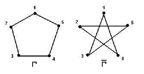
Inspired by the beautiful examples of self-complementary vertex-transitive graphs (a graph that is isomorphic to its complement is said to be self-complementary, see Section 2.6 for a detailed definition) such as the one shown in Figure 1.1, Li and Praeger in [41] introduced the concept of homogeneous factorisations of complete graphs. We shall now define what we mean by a homogeneous factorisation.

This thesis is dedicated to studying homogeneous factorisations of complete graphs with edge-transitive (undirected) factors. More precisely, we look at the situation where there exists a group $G$ that is transitive on the factors of an isomorphic factorisation $\mathcal{E}$ of $K_{n}=(V,E)$ with $M$, the kernel of this $G$-action on $\mathcal{E}$, acting transitively on both vertices and edges of each factor. Thus we have $M<G\leq$ Sym$(V)$ such that:

• •

  For all $E_{i}\in\mathcal{E}=\{E_{1},\ldots,E_{k}\}$ and $g\in G$, we have $E_{i}^{g}\in\mathcal{E}$.

• •

  For any $E_{i}$ and $E_{j}$, there exists $g\in G$ such that $E_{i}^{g}=E_{j}$.

• •

  For each $i$, $M$ fixes $E_{i}$ setwise and is transitive on $V$ and on $E_{i}$.

We shall call such a factorisation an edge-transitive homogeneous factorisation of a complete graph. We also call $(M,G,V,\mathcal{E})$ an arc-transitive homogeneous factorisation if $M$ is arc-transitive on each factor. For convenience, we will often refer to $(M,G,V,\mathcal{E})$ simply as an edge or arc-transitive homogeneous factorisation. Clearly $M$ is a normal subgroup of $G$ (since it is the kernel of the $G$-action on $\mathcal{E}$) and $M=G\cap Aut(\Gamma_{1})\cap\ldots\cap Aut(\Gamma_{k})$. Furthermore, since the group $G$ permutes the factors transitively, it also induces isomorphisms between each pair of the graphs $\Gamma_{i}=(V,E_{i})$ ($1\leq i\leq k)$. (Note that Example 1.1.1 is an arc-transitive homogeneous factorisation $(D_{10},F_{20},V,\mathcal{E})$ of $K_{5}$ of index $2$, where $V=\{1,2,3,4,5\}$ and $\mathcal{E}=\{E\Gamma_{1},E\Gamma_{2}\}$ (see Figure 1.1).)

There are many interesting questions that we can ask pertaining to edge-transitive homogeneous factorisations of complete graphs. However, our point of departure with regards to this topic will be the following natural question.

The focus of this thesis will be centered around the above general question. In Chapter 3, we first study the structure of an infinite class of graphs called the generalised Paley graphs. We will prove in Chapter 4 that they arise as factors of arc-transitive homogeneous factorisations of complete graphs. Also in Chapter 4, we will discuss the general approach used to investigate the structure of the factors of edge-transitive homogeneous factorisations $(M,G,V,\mathcal{E})$ of $K_{n}=(V,E)$. In subsequent chapters (Chapters 5 to 7), we will determine the possible groups $M$ and $G$ in such factorisations, characterise the edge-transitive homogeneous factors that arise, and give a nearly complete and explicit classification. In the case where we do not have an explicit classification (Chapter 7), we are also able to give two infinite families of examples. A more detailed introduction to the main results of this thesis will be given in Section 1.3.

We now give a brief review to the study of graph factorisations and discuss the motivation behind the investigations of edge-transitive homogeneous factorisations of complete graphs.

Investigation into the factorisations of graphs have long been an integral part of graph theory. More important is the study of isomorphic factorisations of graphs and in particular, isomorphic factorisations of complete graphs, which have received considerable attention (see for example [25] and [26]). Isomorphic factorisations of complete graphs are studied for various reasons, but one of the main foci of the research so far has been the study of one-factorisations and two-factorisations of complete graphs (see for instance [7] and [36]).

A one-factor in a graph is a set of edges no two of which are adjacent (that is, they do not share a common vertex) and each vertex of the graph is incident to precisely one of the edges in the set. A one-factorisation of a graph is a partition of the edge set into one-factors. One-factorisations of complete graphs have been widely studied and have implications in many areas, such as tournament scheduling (see [15, p. 566]) and in design theory. We refer readers to the surveys [47, 60] for a detailed account. Two-factorisations of $K_{n}$ coincide with the celebrated Oberwolfach problem, which asks for the existence of factorisations of complete graphs into isomorphic 2-regular graphs (graphs of regular valency 2) on $n$ vertices, whose components are simply cycles of length $c_{1},\ldots,c_{t}$ such that $c_{i}\geq 3$ and $c_{1}+\cdots+c_{t}=n$. Many results had been achieved and we refer readers to [1] for a summary.

Another focus in isomorphic factorisations of complete graphs has been the study of isomorphic Ramsey numbers. For a graph $\Gamma$ containing no isolated vertices and any number $k$, the isomorphic Ramsey number $F(\Gamma;k)$ is defined to be the minimum $m$ such that for every $n\geq m$, $\Gamma$ is isomorphic to a subgraph of every factor of an isomorphic factorisation of $K_{n}$ into $k$ parts. It follows that $F(\Gamma;k)\leq R(\Gamma;k)$ where $R(\Gamma;k)$ denotes the $k$-colouring Ramsey number of $\Gamma$ (which is, the minimum number $m$ such that if we colour the edges of $K_{m}$ with $k$ colours denoted as $\{C_{1},\ldots,C_{k}\}$, then there exists some $i$ ($1\leq i\leq k$) such that $\Gamma$ is isomorphic to some subgraph in $K_{m}$ coloured by $C_{i}$). The most well-studied case is the case where $k=2$ (see [26]), and there are many interesting problems in this area.

The study of homogeneous factorisations of complete graphs was first introduced by Li and Praeger in [41] (see also [40]). In it, the theory of homogeneous factorisations was established and is fundamental source to the development of this thesis. The interest is motivated mainly by the investigations into vertex-transitive self-complementary graphs, which arise as the factors of homogeneous factorisations of complete graphs of index $2$. The study of vertex-transitive self-complementary graphs began with a construction of a family of self-complementary circulant graphs by Sachs in [55]. Since then, vertex-transitive self-complementary graphs have received much attention, see for example [33, 42, 54, 57]. Also, a lot of effort has been made to determine the positive integers $n$ such that there exist vertex-transitive, self-complementary graphs with $n$ vertices (see for example, [2, 38, 48]). In [48], Muzychuk completely determined such positive integers.

One of the major results (Theorem 1.1) of the paper by Li and Praeger [41] is a generalisation of Muzychuk’s result. They proved that a cyclic¹¹ 1 A cyclic homogeneous factorisation of $K_{n}$ is one which the group $G$ induces a cyclic permutation group on the partition $\mathcal{E}$ homogeneous factorisation of index $k$ of $K_{n}$ (where $n=p_{1}^{d_{1}}p_{2}^{d_{2}}\cdots p_{m}^{d_{m}}$, $p_{i}$ are distinct primes and $d_{i},m\geq 1$) exists if and only if, for all $i\in\{1,\ldots,m\}$,

We further note that in [22], the point primitive case for cyclic homogeneous factorisations of complete graphs is studied (that is, where $G$ acts primitively²² 2 See Section 2.3 for definition of a primitive permutation group. on the vertices $V$). They are related to the exceptionality of permutation groups studied in [23].

Our investigation of edge-transitive homogeneous factorisations of complete graphs can also be traced back to the study of arc-transitive self-complementary graphs (which are factors of arc-transitive homogeneous factorisations of complete graphs of index $2$). In [62], H. Zhang gave an algebraic characterisation of all self-complementary, arc-transitive graphs, and showed that they are all Cayley graphs. One family of examples is the well-known class of Paley graphs. In [50], W. Peisert, in an attempt to determine if there are any self-complementary arc-transitive graphs other than the Paley graphs, completely classified, up to graph isomorphism, all finite self-complementary arc-transitive graphs (see Theorem 1.2.1). In his paper [50], Peisert constructed a second infinite family of self-complementary arc-transitive graphs that are not isomorphic to the Paley graphs (except for one case), and called them the $\mathcal{P}^{*}$-graphs. Like the Paley graphs, the $\mathcal{P}^{*}$-graphs are defined on finite fields $\mathbb{F}_{p^{R}}$ where $p\equiv 3$ (mod $4$) and $R$ is even. In fact, by expanding on Peisert’s construction, we are able to construct an infinite family of graphs (where the $\mathcal{P}^{*}$-graphs occur as a special case), called the twisted generalised Paley graphs, that arise as factors of arc-transitive homogeneous factorisations of complete graphs.

We shall present Peisert’s result below.

This thesis originated in the work of H. Zhang [62] in 1992 on arc-transitive self-complementary graphs. However, in our investigation, we use and refine the methodology developed by Li and Praeger in [41] for studying homogeneous factorisations of complete graphs. Just as Peisert was able to complete Zhang’s work, we achieve an almost complete classification of arc-transitive homogeneous factorisations of complete graphs of all indices $k$. Our classification relies on the finite simple group classification through its use of the classification of finite 2-transitive permutation groups. Moreover, our classification specialises in the index 2 case to the theorem of Peisert (Theorem 1.2.1). Finally, on a more ambitious note, it is hoped that by our study of edge or arc-transitive homogeneous factorisations of $K_{n}$, we may be able to shed some light on the computation of lower bounds for some $k$-colouring Ramsey numbers.

In this section, we will give a summary of the important results achieved in this thesis. The main results are found in Chapters 3 to 7. Chapter 3 is based on the paper [46], Chapters 4, 5 and 7 are based on [39] and Chapter 6 is based on [45].

Chapter 3 deals with the structure of the class of generalised Paley graphs, denoted as $GPaley(p^{R},\frac{p^{R}-1}{k})$, which arise as factors of arc-transitive homogeneous factorisations of complete graphs on $p^{R}$ vertices, where $p$ is prime and $R\geq 1$ (see Definition 3.1.1). One of the main results in this chapter says that a connected generalised Paley graph is either a Hamming graph or a normal Cayley graph where its full automorphism group is an affine primitive group.

Furthermore, we determine explicitly the full automorphism group of a class of generalised Paley graphs under certain conditions which are relevant to the study of arc-transitive homogeneous factorisations (see Theorem B below; also see Section 3.1 for details on the notations used). This result will be used in Chapter 7 to show the non-isomorphism between the class of generalised Paley graphs and another infinite family of graphs (the twisted generalised Paley graphs, see Definition 4.4.3) that also arise as factors of arc-transitive homogeneous factorisations of complete graphs.

In the last part of the chapter, we will briefly mention the connection between the generalised Paley graphs and the class of graphs associated with a symmetric cyclotomic association scheme.

In Chapter 4, we will develop the general theory of edge-transitive homogeneous factorisations $(M,G,V,\mathcal{E})$ of $K_{n}=(V,E)$. In particular, we will show that in such a factorisation, the group $G$ is necessarily $2$-homogeneous (Lemma 4.1.1). Then, using the classification of finite 2-transitive permutation groups as well as Kantor’s description of finite 2-homogeneous but not 2-transitive permutation groups [34], we are able to employ a case-by-case approach in our investigation to classify factors arising from edge-transitive homogeneous factorisations of $K_{n}$. We first deal with the case where $G$ is an almost simple group, that is $G$ has a unique minimal normal subgroup that is nonabelian simple, and show that there exists only one example of an edge-transitive homogeneous factorisations of $K_{n}$ where $n=28$ (Proposition 4.2.1). Then we reduce the problem of classifying factors that arise from edge-transitive homogeneous factorisations $(M,G,V,\mathcal{E})$, where $G$ is an affine group, to the problem of classifying factors arising from arc-transitive homogeneous factorisations, where $G$ is affine 2-transitive. Also in the same chapter, we construct two infinite families of examples: the generalised Paley graphs $GPaley(p^{R},\frac{p^{R}-1}{k})$ and the twisted generalised Paley graphs $TGPaley(p^{R},\frac{p^{R}-1}{2h})$. Both graphs arise as factors of arc-transitive homogeneous factorisations $(M,G,V,\mathcal{E})$ of $K_{n}=(V,E)$, where $G\leq A\Gamma L(1,p^{R})$ (and so $n=p^{R}$), that is, $G$ is a one-dimensional affine permutation group acting on the finite field $\mathbb{F}_{p^{R}}$.

In Chapter 5, we will look in detail at the list of affine 2-transitive permutation groups in Theorem 2.2.1. For each class of groups $G$ in that list, we analyse and find out all possible transitive normal subgroups $M$, and use this information to determine the structure of the $M$-arc-transitive factors. We show that many of the examples are disconnected generalised Paley graphs. In other cases, we use Magma [8] to construct the factor graphs (as $M$-orbital graphs) and compute their full automorphism groups. By doing that, we are able to determine their structures more explicitly. The main result in this chapter classifies all factors arising from $(M,G,V,\mathcal{E})$, where $G\leq A\Gamma L(a,q)$ is an affine 2-transitive permutation group with $a\geq 2$ (that is, $G$ is not a one-dimensional affine 2-transitive group). Combining the result (Proposition 4.2.1) from the previous chapter for the case where $G$ is almost simple, we have the following.

(See Chapter 5 for further details on the notations used in Theorem C. Also, part $2(c)$ of Theorem C relies on a result from Chapter 6 which shows that the factors are Hamming graphs.)

In Chapter 6 we show, using representation theory, that one example of an arc-transitive homogeneous factorisation of $K_{n}$ determined in Chapter 5 has factors that are all isomorphic to the Hamming graph $H(9,2)$. We also show that such a factorisation of a complete graph (into Hamming graphs) gives rise to a related edge partition that corresponds to an interesting 2-design (see Theorem 6.3.2).

Chapter 7 deals with the (one) remaining case not covered in Chapter 5: where $G$ is a one-dimensional affine 2-transitive permutation group. By expressing the groups $G$ and $M$ using a standard set of parameters introduced by Foulser in [17] (see also [18]), we give a generic construction (Construction 7.1.10) that will yield all possible arc-transitive homogeneous factorisations $(M,G,V,\mathcal{E})$ where $M,G,\leq A\Gamma(1,p^{R})$ (see Theorem 7.1.11).

We also show that the two infinite families of examples, the generalised Paley graphs $GPaley(p^{R},\frac{p^{R}-1}{k})$ and twisted generalised Paley graphs $TGPaley(p^{R},\frac{p^{R}-1}{2h})$, constructed in Section 4.4 can be derived from this generic construction. Finally, in the last part of the chapter, we will prove that, except for one small example, the graphs from the two infinite families are pair-wise non-isomorphic.

Let $V$ be a finite set of size $n$. A bijection of $V$ onto itself is called a permutation on $V$. The set of all permutations on a finite set $V$ form a group under the operation of composition of mappings. We call this group the symmetric group on $V$ and denote it by Sym$(V)$ or S_n. Any subgroup $G$ of Sym$(V)$ is said to be a permutation group on $V$, and we say that $G$ is a permutation group of degree $n$ if $|V|=n$. We denote the image of the point $v\in V$ under the permutation $\alpha$ by $v^{\alpha}$. Note that by our definition, a permutation group is always finite. It is of course possible to extend the definition of a permutation group to the infinite case, but in this thesis, we will only consider finite permutation groups and finite groups in general.

Let $G$ be a group and $V$ a finite set. An action of $G$ on $V$ is a map $V\times G\longrightarrow V$ written $(v,g)\mapsto v^{g}$, such that

• •

  for every $v\in V$, $v^{1_{G}}=v$, where $1_{G}$ denotes the identity element of the group $G$, and

• •

  for every $g,h\in G$ and $v\in V$, we have $v^{gh}=(v^{g})^{h}$.

The kernel of the action of $G$ on $V$ is defined to be the subgroup of all elements of $G$ which fix each point of $V$. If this kernel consists of just the identity element of $G$, then we say that $G$ acts faithfully on $V$ (or $G$ is faithful on $V$). Otherwise $G$ is said to act on $V$ unfaithfully (or $G$ is unfaithful on $V$).

Note that every subgroup $G$ of Sym$(V)$ acts naturally on $V$. It is easy to see that such an action is faithful. We will always assume that this is the action we are dealing with whenever we have a permutation group.

When a group (not necessarily a permutation group) $G$ acts on a set $V$, a typical element $v\in V$ is moved by elements of $G$ to various other points. The set of these images is called the orbit of $v$ under $G$ or the $G$-orbit containing $v$. We usually denote it by $v^{G}:=\{v^{g}\mid g\in G\}$ but sometimes, we will use $\mathcal{O}$ to denote a typical orbit of $G$ in $V$. Finally, the number of elements in a $G$-orbit $\mathcal{O}$ is called the length of $\mathcal{O}$.

We also call the set of elements in $G$ which fix a specified point $v\in V$, the stabiliser of $v$ in $G$ and denoted it by $G_{v}:=\{g\in G\mid v^{g}=v\}$. Note that $G_{v}$ forms a subgroup of $G$ and is often called the point-stabiliser of $v$.

A group $G$ acting on $V$ is said to be transitive if for any $u,v\in V$, there is some $g\in G$ such that $u^{g}=v$. In other words, $G$ is transitive on $V$ if it has only one orbit, and so $v^{G}=V$ for all $v\in V$. A group $G$ acting on a set $V$ is said to be semiregular if the only element fixing a point in $V$ is the identity. We say that a group $G$ acting on $V$ is regular if $G$ is both transitive and semiregular on $V$.

Let $G$ be a group and let $V=G$. Then each element $g\in G$ induces a permutation $\hat{g}$ of $V$ by right multiplication:

(This is the right regular representation of $G$; see for example [16, Example 1.3.3].) All permutations $\hat{g}$, with $g\in G$, form a permutation group $\widehat{G}<$ Sym$(V)$ (where $V=G$). Furthermore, $\widehat{G}$ is isomorphic to $G$ and is a regular subgroup of Sym$(V)$.

Let $G$ be a group acting on $V$ and $H$ be a group acting on $U$. Then we say that $G$ on $V$ is permutationally isomorphic to $H$ on $U$ if there exist a group isomorphism $\theta:G\longrightarrow H$ and a bijection $\xi:V\longrightarrow U$ such that $(\xi(v))^{\theta(g)}=\xi(v^{g})$ for all $g\in G$ and $v\in V$.

For a positive integer $k$, we use $V^{(k)}$ to denote the set of $k$-tuples of distinct members of a finite set $V$. Suppose a group $G$ acts on $V$. Then $G$ induces a natural action of $G$ on $V^{(k)}$ defined by

for all $(v_{1},v_{2},\ldots,v_{k})\in V^{(k)}$ and $g\in G$. If $G$ is transitive on $V^{(k)}$ under this action, then we say that $G$ is $k$-transitive on $V$. Now let $V^{\{k\}}$ be the set of all $k$-subsets (that is, the subsets of size $k$) of $V$ where $k=1,2\ldots,|V|$. Then $G$ also induces a natural action of $G$ on $V^{\{k\}}$ defined by

for all $\{v_{1},v_{2},\ldots,v_{k}\}\in V^{\{k\}}$ and $g\in G$. The group $G$ is $k$-homogeneous if its action on $V^{\{k\}}$ is transitive. It is not too difficult to see that a $k$-transitive group is necessarily $k$-homogeneous but the converse is not always true.

As a result of the classification of finite simple groups, all finite $2$-transitive permutation groups have been classified up to permutation isomorphism (see [11]). Now if $G$ is 2-transitive, then by a result of Burnside [10, Section 154], $G$ has a unique minimal normal subgroup $N$ where either $N$ is a regular normal subgroup that is elementary abelian ($G$ is an affine group), or $N$ is a nonabelian simple group ($G$ is almost simple).

A group $G$ is almost simple if it has a unique minimal normal subgroup $N$ which is nonabelian and simple. Equivalently, $G$ is almost simple if $N\leq G\leq Aut(N)$ for some nonabelian simple group $N$. This is true since $C_{G}(N)=1$, so $G$ can be embedded in $Aut(N)$ and the image of $G$ under the embedding contains $Inn(N)\cong N$.

We call a group $G$ acting on a set $V$ affine if it has a regular normal subgroup $N$ which is an elementary abelian $p$-group for some prime $p$, say ${\mathbb{Z}}_{p}^{R}$. Such a regular normal subgroup is often written additively, and we usually call it a translation subgroup and denote it by $T$ (and so $T\cong N={\mathbb{Z}}_{p}^{R}$). The set $V$ is identified with a $R$-dimensional vector space over the prime field $\mathbb{F}_{p}$ and the group $T$ is such that for each $x\in V$, there exists a unique $t_{x}\in T$ which acts on $V$ by translation: $t_{x}:v\longrightarrow v+x$ for all $v\in V$. Each affine group $G$ is a semidirect product $T\rtimes G_{0}$ where $G_{0}$, the stabiliser of $\mathbf{0}\in V=V(R,p)$, is contained in $\Gamma L(R,p)$. However, if $G_{0}\leq\Gamma L(R,p)$ preserves on $V$ a vector space of dimension $a\geq 1$ over a finite field $\mathbb{F}_{q}$ (so $q^{a}=p^{R}$), then we may identify $V=V(a,q)=\mathbb{F}_{q}^{a}$ and $G_{0}$ as a subgroup of $\Gamma L(a,q)$. If such case arise, then the affine group $G=T\rtimes G_{0}$ is identified as a subgroup of $A\Gamma L(a,q)$ acting on $V=V(a,q)$ where $a\geq 1$ and $q^{a}=p^{R}$.

The following contains a list of all finite $2$-transitive permutation groups (up to permutation isomorphism) compiled from [20, Theorem 2.9] and [35] (see also [43]). We further refer readers to [16, Section 7.7] for definitions and descriptions of the nonabelian groups $N$ occurring in Theorem 2.2.1 (1).

The next result characterises finite permutation groups that are $2$-homogeneous but not $2$-transitive.

A partition of a finite set $V$ is a set $\mathcal{B}$ of subsets of $V$ such that $\cup_{B\in\mathcal{B}}B=V$ and $B_{1}\cap B_{2}=\emptyset$ for distinct $B_{1},B_{2}\in\mathcal{B}$. Let $G$ be a group acting on a finite set $V$. A nonempty subset $B\subseteq V$ is called a block for $G$ if for every $g\in G$, either $B\cap B^{g}=\emptyset$ or $B=B^{g}$. A block $B$ is said to be trivial if $|B|=1$ or $B=V$. Otherwise, $B$ is called nontrivial. Let $\mathcal{B}$ be a partition of $V$ and $G$ be a group acting on $V$. If $B^{g}\in\mathcal{B}$ for any $B\in\mathcal{B}$ and $g\in G$, then we say that $\mathcal{B}$ is a $G$-invariant partition of $V$. It is easy to see that elements of a $G$-invariant partition $\mathcal{B}$ are blocks for $G$. Moreover, $G$ permutes the elements of $\mathcal{B}$ blockwise and induce a (possibly unfaithful) natural action on $\mathcal{B}$. We say that a group $G$ acting on $V$ is primitive if $G$ is transitive on $V$ and the only blocks for $G$ are the trivial ones. If $G$ is transitive but not primitive on $V$, then $G$ is said to be imprimitive.

The following lemma shows that partitions invariant under a transitive permutation group often arise as orbits set of a normal subgroup.

The structure of finite primitive permutation groups up to permutational isomorphism are described by the O’Nan-Scott Theorem (for example see [51]; see also [44] or [56]). The O’Nan-Scott Theorem essentially provides an identification of several types of finite primitive permutation groups such that, for each type, information is given about the abstract group structure, or the group action, or both. Here, we will briefly describe only three types of finite primitive permutation groups (we refer readers to [51] for further details about the remaining types).

A finite primitive permutation group $G$ on $V$ is of type HA (holomorph of an abelian group) if $G=T\rtimes G_{0}$ is a subgroup of an affine group $AGL(R,p)$ on $V$, where $T\cong{\mathbb{Z}}_{p}^{R}$ is the (regular) group of translations (and we may identify $V$ with a $R$-dimensional vector space over $\mathbb{F}_{p}$) and $G_{0}$ is an irreducible subgroup of $GL(R,p)$. We often call a primitive group of this type an affine primitive permutation group. (Note that the holomorph Hol$(K)$ of a group $K$ is the semidirect product $K\rtimes Aut(K)$, where $Aut(K)$ acts naturally on the normal subgroup $K$. The group $AGL(R,p)$ is Hol$(T)$ where $T\cong{\mathbb{Z}}_{p}^{R}$, so the affine primitive groups are primitive subgroups of holomorphs of elementary abelian groups.)

A primitive permutation group $G$ is of type AS (almost simple) is such that $G$ is an almost simple group.

Finally, to describe the next type of primitive group, we define a special type of group action which we will also often encounter throughout this thesis. Let $H$ be a group, $b>1$ a positive integer and $K$ be a subgroup of the symmetric group $S_{b}$. Then the wreath product $H\ wr\ K$ is the semidirect product $H^{b}\rtimes K$ where elements of $K$ act on $H^{b}$ by permuting the “entries” of elements of $H^{b}$, that is, $(h_{1},h_{2},\ldots,h_{b})^{k^{-1}}=(h_{1^{k}},h_{2^{k}},\ldots,h_{b^{k}})$ for all $(h_{1},h_{2},\ldots,h_{b})\in H^{b}$ and $k\in K$. Now suppose $H\leq$ Sym$(\Delta)$. Then the product action of $H\ wr\ K$ on $\Delta^{b}$ is defined as follows. Elements of $H^{b}$ act coordinate-wise on $\Delta^{b}$ and elements of $K$ permute the coordinates: for $(h_{1},\ldots,h_{b})\in H^{b}$, $k\in K$, and $(\delta_{1},\ldots,\delta_{b})\in\Delta^{b}$,

Bibliography

- [1] B. Alspach, The Oberwolfach problem, in The CRC handbook of Combinatorial Designs (C. J. Colbourn and J. H. Dintz, Eds.), CRC Press, Boca Raton, FL, 1996, 394-395.
- [2] B. Alspach, J. Morris and V. Vilfred, Self-complementary circulant graphs, Ars Combinatoria 53 (1999), 187–191.
- [3] M. Aschbacher, Finite Group Theory, Cambridge University Press, Cambridge, 1986.
- [4] E. Bannai and T. Ito, Algebraic Combinatorics I: Association Schemes, Benjamin/Cummings, Menlo Park, California, 1984.
- [5] Á. Bereczky, Maximal overgroups of Singer elements in classical groups, J. Algebra, 234 (2000), 187-206.
- [6] N. Biggs, Algebraic Graph Theory, Cambridge University Press, Cambridge, 1993.
- [7] A. Bonisoli and D. Labbate, One-factorizations of complete graphs with vertex-regular automorphism groups, J. Combin. Des., 10 (2002), no. 1, 1-16.
- [8] W. Bosma and J. Cannon, Handbook of Magma Functions, School of Mathematics and Statistics, University of Sydney, 1993. (See also http://magma.maths.usyd.edu.au/magma/)
- [9] A. E. Brouwer, A. M. Cohen and A. Neumaier, Distance Regular Graphs, Springer-Verlag, 1989.
- [10] W. Burnside, Theory of Groups of Finite Order, 2nd edition, Dover, New York, 1955.
- [11] P. J. Cameron, Finite permutation groups and finite simple groups, Bull. London Math. Soc., 13 (1981), 1-22.
- [12] P. J. Cameron, Permutation Groups, Cambridge University Press, Cambridge, 1999.
- [13] J. H. Conway, R. T. Curtis, S. P. Norton, R. A. Parker and R. A. Wilson, Atlas of Finite Groups, Clarendon Press, Oxford, 1985.
- [14] P. Dembowski, Finite Geometries, Springer, Berlin, 1968.
- [15] J. H. Dinitz, E. R. Lamken and W. D. Wallis, Scheduling a tournament, in The CRC handbook of Combinatorial Designs (C. J. Colbourn and J. H. Dintz, Eds.), CRC Press, Boca Raton, FL, 1996, 565-578.
- [16] J. D. Dixon and B. Mortimer, Permutation Groups, Springer, New York, 1996.
- [17] D. A. Foulser, The flag-transitive collineation group of the finite Desarguesian affine planes, Canad. J. Math. 16 (1964), 443-472.
- [18] D. A. Foulser and M. J. Kallaher, Solvable, flag-transitive, rank 3 collineation groups, Geom. Dedicate 7 (1978), 111-130.
- [19] C. D. Godsil, Algebraic Combinatorics, Chapman and Hall, New York, 1993.
- [20] G. D. Godsil, R. A. Liebler and C. E. Praeger, Antipodal distance transitive covers of complete graphs, Europ. J. Combin., 19 (1998), 455-478.
- [21] C. D. Godsil and G. F. Royle, Algebraic Graph Theory, Springer-Verlag, New York, 2001.
- [22] R. Guralnick, C. H. Li, C. E. Praeger and J. Saxl, On orbital partitions and exceptionality of primitive permutation groups, Trans. Amer. Math. Soc. (to appear).
- [23] R. Guralnick, P. Müller, and J. Saxl, The rational function analogue of a question of Schur and exceptionality of permutation representations, Mem. Amer. Math. Soc. 162 (2003), no. 773.
- [24] R. Guralnick, T. Penttila, C. E. Praeger and J. Saxl, Linear groups with orders having certain large prime divisors, Proc. London Math. Soc. 78 (1999), 167-214.
- [25] F. Harary, R. W. Robinson and N. C. Wormald, Isomorphic factorisations I: Complete graphs, Trans. Amer. Math. Soc., 242 (1978), 243-260.
- [26] F. Harary and R. W. Robinson, Isomorphic factorisations X: Unsolved problems, J. Graph Theory, 9 (1985), 67-86.
- [27] M.-C. Heydemann, N. Marlin and S. Pérennes, Complete rotations in Cayley graphs, European J. Combin. 22 (2001), 179-196.
- [28] B. Huppert, Character Theory of Finite Groups, Walter de Gruyter, Berlin, 1998.
- [29] B. Huppert, Endliche Gruppen I, Springer-Verlag, Berlin, 1967.
- [30] B. Huppert, Singer-Zyklen in Klassischen Gruppen, Math. Z. 117 (1970), 141-150.
- [31] B. Huppert and N. Blackburn, Finite Groups III, Springer-Verlag, Berlin Heidelberg, 1982.
- [32] I. M. Isaacs, Character Theory of Finite Groups, Academic Press, New York, 1976.
- [33] R. Jajcay and C. H. Li, Constructions of self-complementary circulants with no multiplicative isomorphisms, European J. Combin. 22 (2001), 1093-1100.
- [34] W. M. Kantor, Automorphism groups of designs, Math. Z. 109 (1969), 246-252.
- [35] W. M. Kantor, Homogeneous designs and geometric lattices, J. Combin. Theory Ser. A 38 (1985), 66-74.
- [36] G. Kaplan, A. Lev and Y. Roditty, Regular Oberwolfach problems and group sequencings, J. Combin. Theory Ser. A 96 (2001), 1-19.
- [37] C. H. Li, On isomorphisms of finite Cayley graphs – a survey, Discrete Math. 256 (2002), 301-334.
- [38] C. H. Li, On self-complementary vertex-transitive graphs, Comm. Algebra 25 (1997), 3903-3908.
- [39] C. H. Li, T. K. Lim and C. E. Praeger, Homogeneous factorisations of complete graphs with edge-transitive factors, in preparation.
- [40] C. H. Li and C. E. Praeger, Constructing homogeneous factorisations of complete graphs and digraphs, Graphs and Combin. 18 (2002), 757-761.
- [41] C. H. Li and C. E. Praeger, On partitioning the orbitals of a transitive permutation group, Trans. Amer. Math. Soc. 355 (2003), 637-653.
- [42] C. H. Li and C. E. Praeger, Self-complementary vertex-transitive graphs need not be Cayley graphs, Bull. London Math. Soc. 33 (2001), 653-661.
- [43] M. W. Liebeck, The affine permutation groups of rank 3, Proc. London Math. Soc. (3) 54 (1987), 477-516.
- [44] M. W. Liebeck, C. E. Praeger and J. Saxl, On the O’Nan-Scott Theorem for finite primitive permutation groups, J. Austral. Math. Soc. Ser. A 44 (1988), 389-396.
- [45] T. K. Lim, Arc-transitive homogeneous factorisations, Hamming graphs and affine planes, submitted (also in Research Report No. 2003/21, U. Western Australia).
- [46] T. K. Lim and C. E. Praeger, On generalised Paley graphs and their automorphism groups, preprint.
- [47] E. Mendelsohn and A. Rosa, One-factorizations of the complete graph – a survey, J. Graph Theory 9 (1985), 43-65.
- [48] M. Muzychuk, On Sylow’s subgraphs of vertex-transitive self-complementary graphs, Bull. London Math. Soc. 31 (1999), 531-533.
- [49] R. E. A. C. Paley, On orthogonal matrices, J. Math. Phys. Mass. Inst. Tech. 12 (1933), 311-320.
- [50] W. Peisert, All self-complementary symmetric graphs, J. Algebra 240 (2001), 209-229.
- [51] C. E. Praeger, Finite transitive permutation groups and finite vertex-transitive graphs, in Graph Symmetry (Montrael, PQ, 1996), Kluwer Acad. Publ., Dordrecht, 1997, 277-318.
- [52] C. E. Praeger, The inclusion problem for finite primitive permutation groups, Proc. London Math. Soc. (3) 60 (1990), 68-88.
- [53] C. E. Praeger and J. Saxl, Closures of finite primitive permutation groups, Bull. London Math. Soc. 24 (1992), 251-258.
- [54] S. B. Rao, On regular and strongly-regular self-complementary graphs, Discrete Math. 54 (1985), 73-82.
- [55] H. Sachs, Über Selbstcomplementäre Graphen, Publ. Math. Debrecen 9 (1962), 270-288.
- [56] L. L. Scott, Representations in characteristics , Santa Cruz conference on finite groups, Proc. Sympos. Pure Math. 37 (1980), 318-331.
- [57] D. A. Suprunenko, Self-complementary graphs, Cybernetics 21 (1985) 559-567.
- [58] M. Suzuki, Group Theory I, Springer-Verlag, New York, 1982.
- [59] W. T. Tutte, Connectivity in Graphs, University of Toronto Press, Toronto, 1966.
- [60] W. D. Wallis, One-factorizations of complete graphs, in Contemporary Design Theory: A Collection of Surveys (J. H. Dintz and D. R. Stinson, Eds.), Wiley, New York, 1992, 593-631.
- [61] H. Wielandt, Finite Permutation Groups, Academic Press, New York, 1964.
- [62] H. Zhang, Self-complementary symmetric graphs, J. Graph Theory 16 (1992), 1-5.
- [63] K. Zsigmondy, Zur Theorie der Potenzreste, Monatsh. Math. Phys. 3 (1892), 265-284.