SOLUTION OF THE COINCIDENCE PROBLEM IN DIMENSIONS
Abstract.
Discrete point sets such as lattices or quasiperiodic Delone sets may permit, beyond their symmetries, certain isometries such that is a subset of of finite density. These are the so-called coincidence isometries. They are important in understanding and classifying grain boundaries and twins in crystals and quasicrystals. It is the purpose of this contribution to introduce the corresponding coincidence problem in a mathematical setting and to demonstrate how it can be solved algebraically in dimensions 2, 3 and 4. Various examples both from crystals and quasicrystals are treated explicitly, in particular (hyper-)cubic lattices and quasicrystals with non-crystallographic point groups of type , and . We derive parametrizations of all linear coincidence isometries, determine the corresponding coincidence index (the reciprocal of the density of coinciding points, also called -factor), and finally encapsulate their statistics in suitable Dirichlet series generating functions.
1. Introduction
The concept of a coincidence site lattice (CSL) arises in the crystallography of grain and twin boundaries [15, 43, 48]. Different domains of a crystal across a boundary are related by having a sublattice (of full rank) in common. This is the CSL. It can be viewed as the intersection of a lattice with a rotated copy of itself, where the points in common form a sublattice of finite index (we shall not discuss any situation other than that). Until recently, CSLs have been investigated only for true lattices or for crystallographic packings, for example cubic or hexagonal crystals [43, 25, 27]. Although the subject itself is quite old, no systematic investigation in more mathematical terms has been carried out so far.
With the advent of quasicrystals, many new cases arose, since quasicrystals also have grain boundaries and one would like to know the coincidence site quasilattices [44, 45, 53, 54] and, more specifically, which of them can form twins (or multiple twins, where the angle between the grains is a rational multiple of ). Added impetus is given by the experimental progress made in recent years [20], in particular on the study of twins in icosahedral structures. So, an extension of the CSL analysis to all discrete structures is desirable.
It is the aim of this article to provide the mathematical basis for it, and to display various relevant examples in detail. Though we shall include many proofs, it is not possible to present a complete account here, and we have to refer to original sources several times. Additional material can be found in [11, 40, 3]. Let us briefly outline how this article is organized.
In Section 2, we set the scene for the periodic case and derive various results on the coincidence structure of lattices. As we shall need a generalization to modules later on, most results are formulated to match that.
Section 3 deals with cubic lattices, where the cases of dimensions 2, 3 and 4 are treated explicitly. The groups of coincidence isometries are derived together with the corresponding index formulæ, and the statistics of the CSLs is encapsulated in Dirichlet series generating functions which are related to various Dedekind zeta functions.
Sections 4 and 5 consider quasicrystals. Here, the problem must be split into two parts, one being the coincidence problem for the underlying limit translation module (which is universal and discussed in detail) and the other being a problem specific correction in the projection formalism (which is only briefly outlined). This is followed by some concluding remarks.
Finally, in the Appendix, a closely related problem is presented. While CSLs are special sublattices which depend on metric properties, the number of all sublattices of a given index is an affine property and depends only on the rank. The solution is derived explicitly for arbitrary rank.
2. Preliminaries and some general results
This paragraph focuses on lattices, although many properties could directly be formulated for modules. We prefer this approach, as not every reader might directly want to go beyond the lattice situation. We will then generalize the concepts briefly when we pass on to quasicrystals.
The first concept we need is that of a lattice in -dimensional Euclidean space (or -space for short), where we follow the standard approach, see [17] or [29] for details.
Definition 2.1.
A discrete subset of is called a lattice (of rank and dimension ) if it is the -span of vectors that are linearly independent over . These vectors form a basis of the lattice.
In particular, we can write , and is isomorphic to the free Abelian group of rank . Another rather common (and equivalent) characterization is to say that is a co-compact discrete subgroup of .
Beyond a lattice , we shall also need its dual, , which is given by
Definition 2.2.
.
Here, denotes the standard Euclidean scalar product. The dual is of course also a lattice, since (defined through ) is a basis of , called the dual basis. It is convenient to attach a basis matrix to a lattice , where the -th column of consist of the coordinates of in the standard Euclidean basis . It is clear from Definition 2.2 that, if is a basis matrix for , then is one for .
To proceed, we need the concept of a sublattice. Here, in view of generalizations to come in later chapters, we employ the group structure.
Definition 2.3.
Let be a lattice in . A subset is called a sublattice of when it is a subgroup of finite index. The latter is the number of residue classes or cosets of in , denoted by .
By definition, a sublattice has finite index in its (super-)lattice, and thus shares rank and dimension with it. In particular, is not a sublattice of in this notation. If such a situation occurs, we shall speak of net planes or lattice planes (as ).
For lattices, the index also has a direct geometric meaning: it is nothing but the (inverse) quotient of the volumes of the fundamental domains of the two lattices, as can easily be seen with explicit bases for them. A well known result [17] in this context is the following.
Lemma 2.1.
Let be a lattice in with basis matrix . Then, is a sublattice of if and only if there exists a non-singular integral matrix such that is a basis matrix for . The corresponding index is . ∎
This description of sublattices is indeed helpful as one can now show
Lemma 2.2.
Let be a sublattice of of index . Then, is a sublattice of of index .
Proof: Note that means with integral and , by Lemma 2.1. But is a basis matrix for , and is integral (by the standard formula for the inverse of a matrix). This means by Lemma 2.1. Finally, gives the statement about the indices. ∎
Note that, for , need not be the maximal sublattice of which is a homothetic copy of , as can be seen from the example , . Concerning the dual lattice, one can show another useful result.
Lemma 2.3.
If is a sublattice of , one has , and the corresponding factor groups are isomorphic: .
Proof: By assumption, with integral and non-singular. Consequently, one has and the first statement follows from . The two Abelian factor groups are thus of equal order. Isomorphism follows from the observation that the subgroups of which contain are, by duality and part one of the Lemma, in one-to-one relation with the subgroups of which contain , with preservation of the corresponding indices. ∎
Having prepared the ground, we can now introduce various concepts and results which will be helpful for the coincidence problem.
Definition 2.4.
Two lattices are called commensurate, denoted by , when is a sublattice of finite index of both and .
It is clear that only lattices of the same rank can be commensurate to one another, and one also has
Proposition 2.1.
Commensurateness of lattices is an equivalence relation.
Proof: Reflexivity and symmetry are clear by definition. Finally, and together imply that is of finite index in both and (one way to see this is via suitable use of Lemma 2.2), which implies and hence transitivity. ∎
Proposition 2.2.
Let and be commensurate lattices. Then, and are lattices, and one has the following diagram,
where is written as and the indices satisfy and .
Furthermore, the following equations hold:
Proof: Recall that is defined as
It is the smallest group which contains the lattices and . As , Lemma 2.2 guarantees that is again a lattice because for some .
The claim about the indices is a direct consequence of the second isomorphism theorem for groups [57] giving
As is of finite index both in and , all these factor groups are finite.
The second claim follows directly from the definition of the dual lattice: means for all , hence in particular for all , , and therefore . Conversely, if for , , then and . The other identity follows by duality. ∎
Now we come to the central concept of this article.
Definition 2.5.
Let be a lattice in . An orthogonal transformation is called a coincidence isometry of when . The integer is called the coincidence index of . If is not a coincidence isometry, . We set
If necessary, we shall use the lattice as a subscript for the coincidence index, , but usually we can safely manage without. In this article, we consider only linear isometries, called isometries for simplicity. In more general situations, extensions to affine transformations are necessary, compare [40, App. A], but we shall not use them here. One immediate consequence of Definition 2.5 is
Theorem 2.1.
If is a lattice in , and are subgroups of .
Proof: Let and be in , i.e., and . Clearly, this also implies and . From transitivity, we may conclude that and hence . So, is a subgroup of ; the corresponding statement for is obvious. ∎
Without further information on , one cannot determine the corresponding index , except that we know:
Lemma 2.4.
Let . Then, and .
Proof: The first claim is clear from the group property of . Since is an isometry, its action does not change the volume of fundamental domains, and we obtain the equation
This establishes the claim. ∎
More can be said about the -groups of related lattices. The following is immediate:
Lemma 2.5.
If is a lattice, an orthogonal transformation and , one has the relations and . ∎
Since orthogonal transformations and homotheties commute, the -group does not change (up to conjugation) if one applies linear similarity transformations. This is one step to show that the -group essentially is an invariant of so-called Bravais classes (cf. [50] for details on this concept) – if one disregards non-generic solutions for special representatives. The latter problem does not occur if one deals with irreducible symmetries, such as fourfold symmetry in the plane or full cubic symmetry in . In this article, no other situation shall be discussed.
Lemma 2.6.
Let be a sublattice of of finite index . Then, and, for any isometry out of this group, one has .
Proof: If is a coincidence isometry of , we know that has finite index in and hence also in . As , we see . On the other hand, implies by Lemma 2.2, so also and the two groups must be equal. The second statement follows from and by a comparison of indices. ∎
If we write with , one can say more about the relation between and if respects the cosets in suitable ways. In particular, if is disjoint from the cosets for all , one can also derive that .
The last results on the coincidence groups can obviously be extended to
Corollary 2.1.
Commensurate lattices possess the same -group. ∎
With the above results, one can now also relate a lattice with its dual.
Theorem 2.2.
Let be a lattice in and its dual. Then, and the coincidence index of any orthogonal matrix is the same for both lattices.
Proof: Assume . Then, since and , we have , by applying Proposition 2.2 (specialized to the case , where ) and Lemma 2.3. It also follows that if and only if . ∎
We have now all prerequisites to tackle the coincidence problem for lattices and crystals. While we proceed, we shall need, in particular in the part on quasicrystals, various results from algebraic number theory. It is not possible to present a self-contained description here, but references to the relevant literature shall be given. For general background, we refer to [29, Ch. 1.4], to [30, Chs. XIV–XVII and Ch. XX], and, for a number theoretic approach to quasicrystals in general, to [39].
3. Lattices and crystals: the cubic case
Although there are several cubic lattices, let us first consider the primitive (hyper-)cubic lattice, . With the standard Euclidean basis , it can be written as
As we shall need the term ‘primitive’ later on in a different meaning, we replace it here by the term -type from now on, as compared to -type (for face centred cubic, fcc, and its generalizations) and to -type (for body centred, bcc, and its generalizations).
It is immediately clear that an orthogonal matrix with rational entries only is a coincidence isometry of : one can directly give a lattice which is a common sublattice to both and , namely , where is the denominator of defined through
| (3.1) |
where is the greatest common divisor. On the other hand, as soon as one entry of is irrational, say, no point in the direction of coincides with a lattice point after rotation. This means that we have one lattice direction without any coincidence, hence infinitely many residue classes of the set of coinciding points which therefore is not of finite density, and cannot be a coincidence isometry. So we have
Theorem 3.1.
and . ∎
Having this result for the -type (hyper-)cubic lattices, the obvious next question is what happens for the other lattices with (hyper-)cubic symmetry. The types of such lattices, up to similarity transformations, are as follows.
Theorem 3.2.
In dimensions and , there are precisely three hyper-cubic lattices, namely -type, -type and -type. For and , there is only one such lattice represented by the integers resp. by the square lattice, while in , there are two such lattices -type hypercubic and centred. ∎
A proof can be found in [50]. It is possible, in any dimension, to realize the (hyper-) cubic lattices in such a way that they are commensurate – usually, one works with as representative of -type, with the root (weight) lattice () as representatives of -type (-type) in dimensions , with as centred lattice in -space, and with the usual fcc and bcc lattices in -space (or resp. ), compare [18]. With this convention, the -groups of the (hyper-)cubic lattices in (with fixed) are identical, though the corresponding indices might differ. At present, we do not know the general answer in higher dimensions, but more can be said about the cubic lattices in dimensions , and . So, let us summarize some of those results.
3.1. : the square lattice
Let us first describe the case of the square lattice in more detail, as this is the simplest non-trivial example. Here, we shall be less formal and refer for all the details and proofs to [40] without any further mentioning. First, we restrict the description to rotations, and come to reflections at the end of the section.
The square lattice , embedded in resp. , consists of all integer linear combinations of the two vectors and , i.e., . A rotated copy with results in a CSL of finite index, according to Theorem 3.1, if and only if both and are rational, where is the rotation angle. This gives the well-known relation between coincidence rotations and primitive Pythagorean triples [34]. The group of coincidence rotations is thus explicitly seen to be . To investigate this group, we employ some elementary results from the algebraic theory of quadratic fields [30, Chs. XIV and XV]. In particular, we notice that, with , we can identify with the ring of Gaussian integers (the algebraic integers of the quadratic field , an extension of of degree ):
| (3.2) |
The ring is a Euclidean domain and thus has unique factorization up to units, see [30]. The units ( and its powers) form a group isomorphic to , the rotation part of Aut().
In this setting, a rotation corresponds to multiplication by a complex number . This number can be written as with coprime and of equal norm, i.e., (so, rotates the lattice point into another lattice point, , on the same circle around the origin). We now factorize numerator and denominator into Gaussian primes. They are the rational (or ordinary) primes mod , the factor of (a so-called ramified prime), and the pairs of complex conjugate factors of rational primes mod (where , and is not a unit in ). Clearly, as and are coprime and both divide the same rational integer , only the last type of primes can occur in the factorization, always one (or a power of it) in the numerator and its complex conjugate in the denominator.
As a consequence of the unique factorization property up to units, every coincidence rotation can then be factorized as
| (3.3) |
where (only finitely many of them ), is a unit in (a power of ), runs through the rational (or ordinary) primes congruent to 1 (mod 4), and the , are the (complex conjugate) Gaussian prime factors of . We thus have the (non-trivial!) result that is an infinitely generated Abelian group that nevertheless permits the factorization into a torsion group and a free Abelian group, namely
| (3.4) |
with generators for and with for the infinite cyclic groups. By we mean, as usual, the infinite Abelian group that consists of all finite integer linear combinations in the (countably many) generators. We prefer a multiplicative rather than additive notation here as the coincidence groups will not be Abelian in later examples.
To determine the coincidence index , we observe that it is for the units (i.e., true symmetry rotations) and for the generator (since counts the number of residue classes of the corresponding CSL in ). More generally, due to multiplicativity, is the (number theoretic) norm of the numerator of (3.3), i.e.,
| (3.5) |
This shows the power of the generator approach in this (Abelian) situation. The first few generators with are
These are normalized (by multiplication with a suitable unit) to have argument in , and are shown with denominator (a prime 1 (mod 4)). All other coincidence rotations are obtained by combinations, as indicated in Eq. (3.3).
It is convenient to summarize the possible coincidence indices and the number of CSLs with a given index by means of a generating function. To do so, let denote the number of coincidence rotations of index , which means that counts the different CSLs of index . As a consequence of unique factorization in , is a multiplicative arithmetic function (i.e., and for coprime ), and we can calculate the numbers if we know them for with prime and . This simplification is a nice algebraic result that need no longer hold for the analogous problem applied to planar modules with -fold symmetry when , see [40].
In our present case, due to multiplicativity, a Dirichlet series is an appropriate generating function [1, 56]. To calculate explicitly, we observe that, if is a prime power ( (mod ), ), only the two rotations
lead to CSLs of index , wherefore we have in this case. Now, we can directly calculate the entire generating function through its Euler product representation and obtain:
Proposition 3.1.
The Dirichlet series generating function of the number of CSLs of of index is
A little later, we shall express in terms of -functions. This generating function is not only a succinct way of representing the statistics of CSLs and coincidence indices, it is also a powerful tool for determining their asymptotic properties. For example, it can be used to show (through the determination of the right-most pole of in the complex -plane, which is at , and its residue) that the number of CSLs of with index is asymptotically (and the corresponding number of coincidence rotations is asymptotically ). The possible coincidence indices are precisely the numbers with all prime factors , and we then have
| (3.6) |
where is the number of distinct prime divisors of . Each CSL is itself a square lattice [40, 5], with the index as the area of its fundamental domain. We shall come back to this in a more general context.
Finally, the full group of coincidence isometries, , is the semidirect product of the rotation part (normal subgroup) with the cyclic group generated by complex conjugation ( reflection in the -axis):
| (3.7) |
Here, conjugation of a rotation through an angle by complex conjugation results in the inverse rotation (through ). Let us give a justification of Eq. (3.7). Since (semi-direct product) with the of Eq. (3.7), any planar isometry with can uniquely be written as the product
| (3.8) |
of a rotation through with , the reflection in the -axis (complex conjugation). But leaves the entire lattice invariant, whence is a coincidence isometry if and only if is a coincidence rotation.
The calculation of coincidence indices is also simple in this case. The coincidence index for the reflection is 1. For an arbitrary element of , we either meet a rotation (where we know the result already) or use the factorization of Eq. (3.8) again. Then, the coincidence index is identical with that of its rotation part, so Eq. (3.8) is all that is needed. This solves the coincidence problem for the square lattice completely and we have
Theorem 3.3.
The group of coincidence isometries of the square lattice is
This group is fully characterized by Eqs. (3.3), (3.4) and (3.7). The coincidence index of a rotation is given by Eq. (3.5), while that of a reflection (3.8) equals the index of its rotation part. The corresponding Dirichlet series generating function is from Proposition 3.1. ∎
3.2. A short digression on a hierarchy of problems
It is the intention of this paragraph to shed some more light on the coincidence problem and how it relates to similar questions. We shall explain it for the square lattice in an informal manner.
To this end, let us start with the question of how many sublattices of have index – without any further restriction. Let us call this number . Clearly, (only itself is sublattice of index 1) and (counting two different rectangular sublattices and one square sublattice). In general, when are coprime, and one can derive, either from the Appendix or from [51, Lemma 2 on p. 99], the general result
with generating function
| (3.9) |
Here, is Riemann’s zeta function, compare [30]. From this, it can be shown that the number of sublattices with index grows, on average, linearly as , compare [30, Thm. 324]. These results are, of course, affine in nature and apply to any lattice of rank 2, and to any free Abelian group of rank 2 (counting the different subgroups of index ).
Let us look for metric properties by asking how many of the sublattices of of index are actually square lattices (see [4, 8, 9] for various generalizations of this question). This number can be obtained by counting the lattice points on circles of radius (hence counting solutions of the Diophantine equation ) and afterwards dividing by 4 (the order of , the rotation part of the point symmetry group of ). The result is given in Chapters 16.9, 16.10 and 17.9 of [30] and leads to the Dirichlet series generating function
| (3.10) |
where here and in what follows is the Dedekind zeta function of the quadratic field , compare [49, 63, A. 14 on p. 251]. The average value of the coefficients of is constant, namely , which follows either from the asymptotic properties of the generating function near its right-most pole (at ) or just from counting one quarter of the lattice points inside the circle of radius , which is to leading order in .
In the last case, some of the square lattices fail to be primitive (such as etc.), i.e., whenever the sublattice is an integer multiple of or one of its primitve sublattices. If we exclude those, primes are impossible as divisors of the index , and some solutions of also drop out (whenever the index is divisible by a square). Now, the generating function reads
| (3.11) |
and the average number of primitive square sublattices of index is given by . This can be determined by counting one quarter of the visible points [1] in the circle of radius , which is .
Still, not all primitive square sublattices are CSLs – they only are if the index is odd. This finally results in the generating function of the coincidence problem described above, namely
| (3.12) |
where the average number of CSLs of index is . This equation expresses the Dirichlet series generating function in terms of zeta functions. Similar formulas will also appear in later examples. We hope that this short digression has put the problem in a broader perspective. Let us now climb up to higher dimension where the picture changes significantly because is no longer Abelian for .
3.3. : the three cubic lattices
In this paragraph, we shall use the notation for the -type (fcc), -type, and -type (bcc) cubic lattices, respectively. In particular, . Let us start with this and write the lattice as . We already know that (other isometries might also lead to coincidences, but not to a CSL of full rank 3). The subgroup of rotations with index 1 is the rotation symmetry group of the cube of order 24, , cf. [2] for details.
As is well known, is a direct product, where is the centre of . Consequently, we can restrict our attention to pure rotations, as reflections may be written as a product of a rotation with (note that ). At this point, we introduce quaternions , see [32, 22, 30], and Cayley’s parametrization [33] with real numbers ,
| (3.13) |
where is the so-called reduced norm of the quaternion . In particular, the multiplicative group of quaternions of norm , which form the unit sphere , provides the usual double cover of the rotation group , via the group homomorphism (since ).
As we are interested in rotation matrices with rational entries (i.e., in the subgroup ), we consider Cayley’s parametrization with integers , and choose them coprime, i.e., . We call such quaternions primitive. This way, we parametrize the entire group , and obtain each element of it exactly twice (again because of ). With this approach, one obtains the following result.
Proposition 3.2.
Consider and let be parametrized by a primitive quaternion . Its coincidence index is the denominator of as defined in Eq. (3.1). It is the “odd part” of ,
where is the largest integer such that divides .
Before we prove the statement, let us remark that the necessity for the division by in Proposition 3.2 stems from the fact that some primitive quaternions (such as or ) have norms that are not coprime with the matrix entries of . A closer inspection, using results of [32], shows that only the exponents are possible.
Proof: Consider with primitive and . Define the vectors
which all have integer preimages under , and the matrices
Now, each can be read as a basis matrix of a lattice that is a sublattice of both and , hence it is also a sublattice of the CSL . Consequently, the coincidence index must divide each of the determinants . As was primitive, must therefore divide . Since trivially also divides the third power of (which is odd), we have .
To establish the claim, it is now sufficient to show that also . Observe that due to , as in the proof of Lemma 2.4. Since, by definition of the denominator,
the lattice contains a vector of the form with a primitive vector , i.e., with and and . This implies that the number of cosets of in must be a multiple of , so that . ∎
In particular, this reproduces the well-known result [24, 25] that runs precisely through all odd integers, i.e., .
Cayley’s parametrization has the nice property that gives the (generic) rotation axis of ,
| (3.14) |
while the rotation angle follows from , so
| (3.15) |
One can easily construct all solutions for small indices explicitly, while the case gives all coincidence rotations through as described by Lück [34]. If is the number of coincidence rotations of index , the arithmetic function once again counts the different CSLs of index . This function is multiplicative as a consequence of the fact that integer quaternions11 1 They constitute the Hurwitz ring of quaternions of the form with all even or all odd. have unique left (and right) factorization up to units22 2 They are the quaternions (and permutations) and . Together, they form a group that is the double cover of the symmetry group (rotations only) of the regular tetrahedron, see [9]., see [58, 10] for details. Its calculation amounts to counting the representations of an integer as a sum of squares, compare [32, Ch. 11] or [30, Ch. XX], and to observe the relation between and . This results in
Proposition 3.3.
The Dirichlet series generating function for the number of CSLs of of index reads
| (3.16) |
With this generating function, one can again determine the asymptotic behaviour of . The result is that the number of CSLs of index is asymptotically given by , and the number of coincidence rotations with index by .
To expand on the systematics of our generating functions, let us remark that Eq. (3.16) can be rewritten as
| (3.17) |
where is the zeta function of the Hurwitz ring of integer quaternions, compare [49, 63, A. 15 on p. 252]. It is the generating function for the number of non-zero right ideals of the ring , which is a maximal order of the standard quaternion algebra over .
This is not quite the end of the story. Coincidence rotations of a given index can be collected into equivalence classes of rotations related by the action of the point symmetry or, more generally, of . This requires a double coset analysis that is described in [26, 58]. It turns out that inequivalent CSLs of with the same index occur for the first time at .
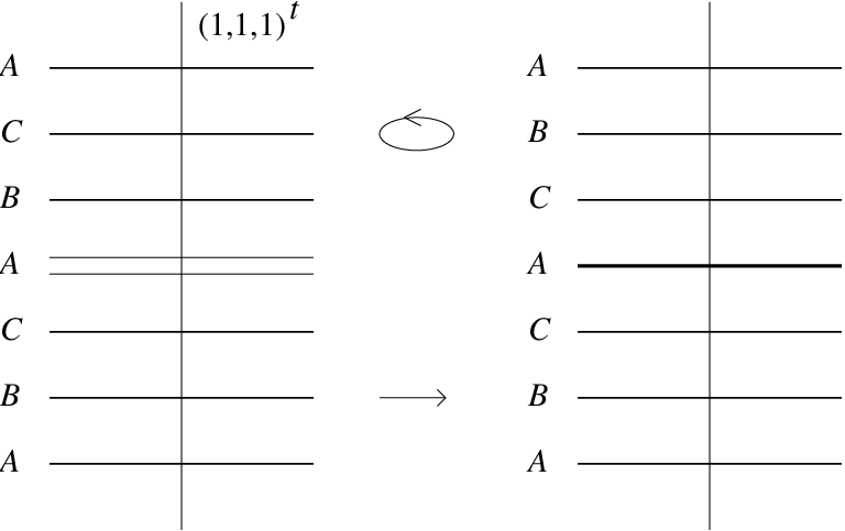
Also, describing the fine structure of a coincidence rotation requires an analysis of the lattice planes perpendicular to the rotation axis. For example, the (unique) equivalence class for can be represented by , i.e., a rotation through around . Here, three layers are stacked periodically (with period ), with perfect coincidence in one (called , which is therefore an ideal grain boundary), but none in the other two (called , which are interchanged in type by the rotation). So, this coincidence rotation can be used to create a twin that shows up as a change in the stacking sequence, see Figure 1.
Let us take a short look at the other cubic lattices, and (from now on, we use indices to distinguish the three cubic lattices). They possess the same group of coincidence isometries as ,
| (3.18) |
but even more, one has
Proposition 3.4.
In , the coincidence index of an orthogonal matrix is the same for all three cubic lattices.
Proof: We can apply Lemma 2.3. From the inclusion
| (3.19) |
we know that and . But from Theorem 2.2, because in this setting. Since is always odd, we can either have or .
However, as and have the same point symmetry, implies , and cannot possess coincidence isometries of index 2. From the multiplicativity of the number of CSLs of index , see [58, 10], it then follows that no CSL of can have even index, hence . ∎
One can see the second step also without reference to the multiplicativity of the CSL counting function. Observe that , with . These two cosets have disjoint shells, and one can check that coincidence rotations produce coinciding points in both shells with equal density, which then implies that .
Nevertheless, there are specific differences in the coincidence structure of the three cubic lattices. They show up in different layer arrangements [25], but details go beyond the scope of this article.
3.4. : the two hypercubic lattices
In four dimensions, there are only two hypercubic lattices (-type and centred, represented by and ), and they confront us with a different situation that occurs in no other dimension: the centred lattice, , has a larger symmetry than its partner of -type, . The dual lattice of , the weight lattice , is equivalent to (through a rotation followed by a homothety) and need not be considered separately, compare [18].
Let us start with the description of the coincidence structure of . First, we observe that quaternions give us again a helpful parametrization of rotations [22, 33], where we now need a pair . The corresponding matrix is defined through
where stands for the transpose of the quaternion (and is thus a column vector). With and , one finds the -matrix
which has
and satisfies the orthogonality relation
Consequently, results in a 4d rotation matrix, and the group homomorphism : is onto. It provides a twofold cover of the rotation group [33], with .
From here, we can find a parametrization of if we start from two non-zero primitive integer quaternions (i.e., each quaternion has the form with and ). Then, if we consider the matrix
| (3.20) |
we see that it is an element of if and only if is a square in , in which case we call the pair of integral quaternions admissible. But with all admissible pairs of primitive quaternions, we actually exhaust , and obtain each element twice (due to ).
From Theorem 3.1, we already know that . As in the previous cases, it is sufficient to treat rotations, since reflections can be written as a product of a rotation with a special reflection that leaves invariant – in complete analogy to the situation in the square lattice ( is a semi-direct product). So, we need to know the coincidence index of an arbitrary rotation . This is not just the denominator of , but given by the following result, see [59, 14] for a proof.
Proposition 3.5.
Let be an admissible pair of primitive integral quaternions, and let denote the index defined above in Eq. (3.2). Then, the matrix has coincidence index
| (3.21) |
Here, denotes the least common multiple, and the subscript refers to the (face-) centred lattice . With this formula, it is now a combinatorial problem to determine the number of coincidence rotations of a given index and, dividing by 576 (the order of the rotation symmetry group of ), also the number of different CSLs of of index . As follows explicitly from Eq. (3.21) and also from the unique factorization of integral quaternions, is again a multiplicative function, so that we only need to calculate it for a prime power.
Starting from Eq. (3.21) and counting the possibilities to contribute to , it is not difficult to derive (for ) the explicit expression
| (3.22) |
with the of the 3d cubic case in Eq. (3.16). An empty sum is to be understood as , and denotes Gauß’ brackets. The result is (see [59] for a proof)
This fixes the Dirichlet series generating function and one obtains
Proposition 3.6.
The Dirichlet series generating function for the numbers of CSLs of index in the root lattice reads
| (3.23) |
Again, the possible indices are precisely all odd integers, . A comparison with the cubic case in -space reveals the remarkable identity
| (3.24) |
where is the generating function of Eq. (3.16). This makes is rather easy to calculate the asymptotic behaviour from that in dimensions. The right-most pole of is at , so one obtains that the number of CSLs of index grows asymptotically as (note that is known to be irrational, but its value is only known numerically). For the number of coincidence rotations with index , one has to multiply by . Another consequence of Eq. (3.24) is the formula
| (3.25) |
which follows from the convolution theorem of Dirichlet series and allows for a simple and efficient calculation of the numbers .
Having described the root lattice , the (face-)centred cubic lattice in four dimensions, we now turn to the slightly more complicated case of the -type cubic lattice, . From the inclusion
| (3.26) |
and the result that and have the same index formula, see Theorem 2.2, we get and . But is always odd, so either or . Here, in contrast to the situation in -space, both possibilities arise. The point symmetry group of is larger than that of , with
| (3.27) |
Consequently, one third of the elements of are symmetries of while the others result in coincidence isometries of . They turn out to have index . In going from here to the number of CSLs of index , it is clear that we have , and for . The multiplicativity (which needs to be proved, e.g., similarly to the arguments given in [59]) of then gives the general answer
This can now easily be summarized as follows.
Proposition 3.7.
The Dirichlet series generating function for the number of CSLs of index in reads
| (3.28) |
Note that, in comparison to the case, the number of CSLs grows faster by a factor of , while the number of coincidence rotations grows slower by a factor of , due to the smaller point symmetry group of .
This calculation was actually possible without giving the corresponding index formula first, by using the multiplicativity of . Since , there must be a different index formula for , and indeed one obtains, for an admissible pair of primitive integral quaternions (see [59] for a proof)
| (3.29) |
At this point, we close our description of the coincidence structure of lattices and turn to the perhaps more interesting case of quasicrystals.
4. Coincidence isometries for modules
So far, we have described the case of lattices and crystals. For the treatment of quasicrystals, we have to extend our concepts to -modules, embedded in Euclidean space, which are not necessarily discrete any more.
Definition 4.1.
A subset of is called a -module, of rank and dimension , when it is the -span of vectors (the basis of the module) that are linearly independent over , but span over .
Clearly, we must have , and a module with is a lattice. As a group, a module of rank is isomorphic to the free Abelian group of rank – so we may consider such modules as special geometric realizations of free Abelian groups.
At this point, the concepts of submodule, commensurateness, and that of coincidence isometry and index, are defined in exact analogy to Section 2, so there is no need to repeat them here. We only note that the set of coinciding points is now a module rather than a lattice, wherefore we call it a coincidence site module, or CSM for short. A bit more care is needed for the definition of a dual module. Let us first observe
Lemma 4.1.
For every module of rank and dimension , there is a lattice such that is the one-to-one projection of into .
Proof: Out of the basis of , we can pick -linearly independent vectors which span over , say w.l.o.g. They span a lattice in . The statement is now obvious as we can add one new dimension for each basis vector remaining. This can always be done in such a way that the projection is one-to-one on . ∎
It is an obvious idea to try to define a dual object for a module through a lift to a lattice because then is well-defined and can be projected down again. Unfortunately, this is neither unique nor satisfactory, as it can happen that the object defined this way is a module of smaller rank than the original one. If, however, there is some additional structure (e.g., irreducible symmetry), such a lift can be made essentially unique and the dual object is well-defined, see [38, 39] for relevant examples in our present context. If this situation applies, it is again true that a module and its dual module share coincidence group and index formula.
In what follows, we concentrate on examples that are connected with the golden ratio, . The modules that will appear are invariant under multiplication by or a power thereof. So, it might be instructive to see how the construction of a dual module works here. The simplest example is the ring of golden integers
| (4.1) |
which is the ring of algebraic integers in the quadratic field , but can also be seen as a -module of rank and dimension in . The special structure that helps in this case is the existence of an automorphism ′ of , called algebraic conjugation, which maps to its algebraic conjugate (hence the name) and thus to . Now, the set
| (4.2) |
is a lattice in -space , from which one obtains by projection into . In , has a well-defined dual lattice, , and neither nor has a lattice direction parallel to . But then, we define the dual module by the projection of into (which, in this case, gives ), and this object is unique in the sense that any other embedding of into which maps algebraic conjugation to a lattice automorphism will result in the same dual object .
Though examples in higher dimensions are more complicated (and will require more than just one automorphism), the basic idea is similar. In particular, it applies to all quasicrystals of interest, compare [39]. It turns out that root lattices [18] prove extremely handy here [6]. Let us now illustrate the coincidence problem for noncrystallographic patterns by a seris of examples related to fivefold symmetry. For further material on planar structures with -fold symmetry, we refer to [11, 40, 5].
5. Modules and quasicrystals: the root systems , and
Among the many possible quasiperiodic tilings, those attached to fivefold symmetry are of particular interest, especially in view of their application in solid state physics. Let us therefore start from the exceptional Coxeter groups (usually called ), and [31] shown in Fig. 2. They are the symmetry groups of certain regular polytopes [19], namely of the regular decagon ( in Schläfli’s notation), the icosahedron (or dodecahedron ) and the regular 600-cell (or the regular 120-cell ), and are of order 20, 120 and 14400, respectively.

The corresponding root systems (up to normalization) are given by the vectors which point to the 10 vertices of a regular decagon (), to the 30 vertices of the icosidodecahedron (), and to the 120 vertices of the regular 600-cell in 4-space (), see [38] or [31] for details. The -spans of these root systems define -symmetric modules, which can be seen as projections from the root lattices , and . In particular, they all have well-defined duals, though we do not expand on this question here – it is discussed in detail in [38].
Having set the scene, we can now describe the coincidence structure of these modules (and some closely related ones). We shall also briefly discuss the connection to quasiperiodic tilings.
5.1. : Coincidence rotations for tenfold symmetry
Let us consider a 2d quasicrystal with tenfold symmetry, the Tübingen triangle tiling [7] of Fig. 3, say. As mentioned earlier, the coincidence problem splits into two parts: first, the coincidence problem for the underlying -module (which is the limit translation module [12] of the tiling) and second, the correction, due to the acceptance domain, of the coincidence indices obtained in this way [40]. Here, we discuss in detail only the first part.

In the complex plane, the tenfold module of rank 4 over [35] can be written as the direct sum
| (5.1) |
with a fifth root of . As such, is the ring of algebraic integers in the cyclotomic field (a field extension of of degree ). Again, prime factorization is unique up to units [55]. One can now go through essentially the same argument as in the case of the square lattice. The primes in are slightly more complicated, but only those dividing a rational prime can enter the factorization of with coprime. The result is [40]:
Proposition 5.1.
Every coincidence rotation written as of the standard tenfold symmetric module can be factorized as
| (5.2) |
where is a th root of and thus a unit in , and only finitely many of the exponents , are different from .
This factorization is slightly more complicated than that in the case of the square lattice, as we have two independent generators for each basic index . This originates in the fact that these (rational) primes are the product of cyclotomic primes in which form two independent pairs of complex conjugates.
The index of a rotation is
| (5.3) |
and the group of coincidence rotations has the form
| (5.4) |
Thus, in spite of the more complicated factorization, the structure of the coincidence group remains simple (as it does for other planar symmetries, compare [40, 5]). Let us give two examples before we continue. and are the smallest non-trivial indices, with two generators each. With , they can be written as follows:
| (5.5) |
Coincidence reflections can be described as products of rotations with the reflection in the -axis, exactly as in the case of the square lattice, so we need not repeat that argument here.
If denotes the number of coincidence rotations of index , the multiplicative function actually counts the number of different CSMs of index . We then obtain, with :
Proposition 5.2.
The Dirichlet series generating function for the coincidence problem of the tenfold symmetric module of rank in the plane reads
| (5.6) |
Here, is the Dedekind zeta function [55] of the cyclotomic field , while is the zeta function of the maximal real subfield, , see also Eq. (5.10) below.
All CSMs are scaled versions of and the number of CSMs of index is asymptotically (while the number of coincidence rotations with index is times as large).
How do these results apply to the coincidence problem of the tenfold symmetric triangle tiling? The latter can be obtained through projection from the root lattice with a regular decagon as its window [7]. A coincidence in the set of vertex points occurs if and only if there is a coincidence in the module such that the image point in internal space lies both in the original window and in an appropriately rotated window. A consequence of this is that the coincidence group of the tiling is still , but also that the -factor or “index” of each group element is normally smaller than its index in by a correction factor close to (depending on the group element).
This is called the window correction factor, and has to be calculated for each tiling separately, as a function of the rotation angle. It also explains why the set of coinciding points forms a tiling of slightly different type from the original one, a small proportion of the points of the original tiling being missing from it. In fact the term “index” for the reciprocal of the fraction of coinciding points is no longer appropriate in this setting, as it neither has a purely algebraic interpretation, nor is an integer any more. Details of this and the determination of the rotation angle in internal space by means of algebraic conjugation are given in [40]. In many examples, in particular when the windows are regular polytopes, the maximal error is so small (at most of the order of a few percent) that one can safely ignore it and work with the module index instead.
5.2. : the icosahedral modules of rank 6
Icosahedral quasicrystals are of particular interest, and one would like to know their coincidence structure in detail [54, 41]. We restrict our discussion to the investigation of the 3 different 3d icosahedral modules of rank 6 over [47] and again omit the determination of the window correction. We shall call the modules , , for -, - and -type, respectively33 3 This terminology originates from the fact that these modules can be obtained as projections of the three types of hypercubic lattices in -space, , , and .. They are spanned by the orthonormal basis with coefficients , , as follows:
| (5.7) | |||||
The use of an orthonormal basis may be a bit surprising at first sight, but it will prove useful in a moment. It is possible in this simple form because are chosen parallel to mutually orthogonal twofold axes of the icosahedron. In this setting, is the -span of the root system of type , and hence a -module of rank and dimension . It actually also is a -module (of rank ), which is also true of , but not of . This relates to the fact that and are invariant under multiplication by , while is only invariant under multiplication by .
To describe the coincidence rotations (in the orthogonal basis), Cayley’s parametrization can again be used. Our first assertion is that the coincidence group is the same for all three modules:
Proposition 5.3.
Proof: Observe the relations and . These modules all possess the same -group, and this obviously is by the same type of argument we have used previously in the discussion of the (hyper-)cubic lattices. ∎
The unit quaternions , , together with all even permutations and arbitrary sign flips form a group of order 120 which is the usual double cover [31, 36] of the icosahedral group . The icosian ring , see [36] for details, consists of all integral linear combinations of elements in and is a maximal order with unique (left- or right-) factorization in the quaternion algebra over the field . One finds the relation , and our second assertion is the index formula for a coincidence rotation , again for all three modules:
| (5.8) |
where the argument on the right hand side is always a number in and its norm is defined by . We use the convention that the gcd is always a positive number. The indices run through all positive integers of the form with integral and . These are the numbers all of whose prime factors congruent to 2 or 3 (mod 5) occur with even exponent only. (They can also be characterized as the positive numbers of the form with integral and , as used in [41].) For , one finds the list of numbers
which covers the cases known from [54].
If is the number of coincidence rotations of index , is the number of different CSMs of index . Since the icosian ring is a maximal order with unique (left- or right-) factorization [46, 52], is again a multiplicative function, i.e., and whenever are coprime. Furthermore, with , one finds
Then, if (5),
Finally, if (5),
This fully determines the generating function of .
Proposition 5.4.
The Dirichlet series generating function for the number of CSMs of an icosahedral module from Eq. (5.7) is given by
The number of CSMs of index is asymptotically (while the number of coincidence rotations with index is times as large).
The function can be expressed in terms of zeta functions as
| (5.9) |
with the quadratic field , the -function of the icosian ring, and
| (5.10) |
A more complete description of the icosahedral case, which requires a certain level of mathematical machinery and various results from algebraic number theory, will be given in [10].
5.3. Short digression on a related cubic module of rank 6
Crystals and quasicrystals are specific examples of ordered phases with longe-range order, but there are many other ones. Incommensurate structures are also widely studied in the literature, and they are also connected to modules rather than lattices. It is an obvious question what happens to such modules if they still have cubic symmetry (and hence dimension 3), but rank 6. There are 6 types of such modules, called , , , , , and in a suggestive notation. Let us consider the case in a bit more detail. It is clear that is an example of it if we demand (otherwise, the rank would not be 6).
So, let us assume that is irrational. Then, and we can write the module as . Generically, the -group will be that of itself (with the index squared), because, if is not algebraic, there is no rotation which brings a point of into coincidence with one of . This changes quite a bit if is algebraic. A case of particular interest in our context is that of , where we get the module
This module has the same -group as the three icosahedral modules above, , but a different index formula. In fact, in complete analogy to the cubic lattices, one can prove that
| (5.11) |
Here, is defined w.r.t. and hence a number of the form , is the norm in as used above, and the absolute value is needed because the denominator is only defined up to units in , which are the numbers with norm .
It is clear from Eq. (5.11) that the set of indices is the same as in the icosahedral case, i.e., all positive integers which are representable by the integral quadratic form . More surprising is the result that the generating function is very similar: differences only occur for indices which are divisible by 4. Explicitly:
| (5.12) |
Due to the prefactor, the number of CSMs of index grows faster than that of the icosahedral case by a factor of , while, due to the different point symmetry groups, the number of coincidence rotations grows slower by a factor of .
5.4. : the icosian ring as -symmetric module
Our final example is the icosian ring itself, compare [36], viewed as the module obtained as the -span of the root system of type . It is the limit translation module of a highly symmetric 4d quasicrystal studied in [23], and can also be obtained by projection of the root lattice to a 4d subspace that is invariant under the action of the symmetry group of the regular 600-cell (which, in turn, is isomorphic to the Coxeter group ), see [9, 37] for more.
The solution of this case proceeds in close analogy to that of , details will appear in [14]. The coincidence group obviously is , and in order to obtain a parametrization of its rotation matrices, we are again using admissible pairs of quaternions . This now means that must be a square in . This gives some slight extra complication from the arithmetic of , compare [21], as rational primes (5) split into a product of two -primes which are algebraic conjugates of one another, but not associates. Consequently, Eq. (3.22) has a counterpart in the present case that has to be modified for such primes by an extra factor 1/2 on the right hand side, while it is true in its unaltered form for all other primes. The result is a multiplicative function which counts the CSMs of of index . It is specified by , and, for , by
if (5), one has
Finally, for (5), one obtains the rather lengthy expression
Although this looks a bit nasty, the corresponding Dirichlet series has the nice form
| (5.13) |
which resembles the situation of the root lattice described above, see [14] for more. In particular, one can again use the recursion (3.24) to calculate the coefficients directly from those of the icosahedral case. The last equation also permits the determination of the asymptotic behaviour, compare [9, Appendix]. With the methods described in [55, pp. 29–31], applied to , one can calculate the values of explicitly for . This finally gives that the number of CSMs of index is asymptotically
where has to be calculated numerically.
6. Concluding remarks
In this contribution, we have shown how the so-called coincidence problem can be reformulated in a mathematical setting and then solved algebraically in dimensions 2, 3 and 4. Various examples have been treated explicitly, and it remains a simple exercise to work out tables of all coincidence rotations with small indices that could be relevant experimentally.
Rather obvious is the question for generalizations to higher dimensions. One might hope that at least the root lattices could be treated in full generality, but there are complications from various sources. First of all, we do not have suitable generalizations of quaternions at our disposal (and they proved extremely handy in our treatment), and second, we depended on unique factorization in one way or another – and this does not generalize to arbitrary lattices or modules.
Another obvious question emerges from the observation that we have so far only dealt with linear isometries, while for various reasons affine extensions are necessary, in particular for a satisfactory formulation of the problem in the context of more general Delone sets. Though some preliminary investigations exists [40], more has to be done in this direction.
Appendix A The number of sublattices of a given index
Given a free Abelian group of rank , one might like to know how many different subgroups of (finite) index exist. Of course, they are free and of rank again, but here we want to count them separately, not up to isomorphism. Let us call that number and derive a recursion relation for it44 4 This derivation is partially based on notes by P. A. B. Pleasants. Since, for fixed , is a multiplicative function in , this will allow the derivation of a closed formula both for and for its Dirichlet series generating function.
Since any free Abelian group of rank is isomorphic to , we can treat the latter case without loss of generality, but with some benefit from the geometric setting. Let be a sublattice of of index . Next, define a new lattice by intersection with an -dimensional hyperplane. Then, is a sublattice of of finite index , where we must have .
At this point, we also know that can be generated by and some vector with (this is nothing but the completion theorem for bases applied to this situation). Next, we observe that we can actually calculate the number of lattices that give rise to the same ,
because is the number of residue classes of in . Now, summation over all possibilities for results in the following simple recursion formula which is well-known, see [49, 63, A. 13 on p. 251], but rather difficult to locate:
| (A.1) |
One can now derive a closed expression for , namely
Proposition A.1.
.
Here, the sum runs over all -tuples of positive integers subject to the restriction that .
Proof: It is clear that . From Eq. (A.1), we get by induction
which completes the argument, see [28, 60] for alternative approaches. ∎
Let us determine a generating function for . Due to the multiplicativity of in , one would like to have a Dirichlet series generating function. This can be found as follows, using again the recursion relation (A.1).
The middle line is the product formula for two Dirichlet series generating functions, applied to our special case. From this calculation, one gets the recursion
| (A.2) |
Since there is only one sublattice of index for the case , we have and thus, by induction, one obtains
Proposition A.2.
. ∎
In particular, this gives , which is the well-known generating function for the divisor function .
Let us close this appendix with a short remark on the asymptotic behaviour of the coefficients. has its rightmost pole at , with residue (if ) and (if ). Then, the number of sublattices with index is asymptotically given by , while the average number of sublattices with index grows like .
Acknowledgements
It is a pleasure to thank P. A. B. Pleasants for his cooperation, M. Schlottmann for critically reading the manuscript, R. V. Moody, J. Roth, and A. Weiss for helpful comments, and the Fields Institute for Research in Mathematical Sciences for financial support during a stay in fall 1995 where this manuscript was written. I am also grateful to the MASCOS centre at the University of Melbourne for support during a stay in 2006, where the manuscript was revised and updated, and to P. Zeiner for various suggestions for improvements.
References
- [1] Apostol, T. M. (1984), Introduction to Analytic Number Theory, Springer, New York; 5th corr. printing (1998).
- [2] Baake, M. (1984), Structure and representations of the hyperoctahedral group, J. Math. Phys. 25, 3171–3182.
- [3] Baake, M. (1996), Algebraic solution of the coincidence problem for crystals and quasicrystals, in: Statistical Models, Yang-Baxter Equation and Related Topics and Symmetry, Statistical Mechanical Models and Applications, eds. M. L. Ge and F. Y. Wu, World Scientific, Singapore, pp. 31–40.
- [4] Baake, M., and Grimm, U. (2004), Bravais colourings of planar modules with -fold symmetry, Z. Krist. 219, 72–80; math.CO/0301021.
- [5] Baake, M., and Grimm, U. (2006), Multiple planar coincidences with -fold symmetry, Z. Krist. 221, in press; math.MG/0511306.
- [6] Baake, M., Joseph, D., Kramer, P., and Schlottmann, M. (1990), Root lattices and quasicrystals, J. Phys. A: Math. Gen. 23, L1037–L1041.
- [7] Baake, M., Kramer, P., Schlottmann, M., and Zeidler, D. (1990), Planar patterns with fivefold symmetry as sections of periodic structures in -space, Int. J. Mod. Phys. B4, 2217–2268.
- [8] Baake, M., and Moody, R. V. (1998), Similarity submodules and semigroups, in: Quasicrystals and Discrete Geometry, ed. J. Patera, Fields Institute Monographs, vol. 10, AMS, Providence, RI, pp. 1–13.
- [9] Baake, M., and Moody, R. V. (1999), Similarity submodules and root systems in four dimensions, Can. J. Math. 51, 1258–1276; math.MG/9904028.
- [10] Baake, M., Pleasants, P. A. B., and Rehmann, U. (2006), Coincidence site modules in -space, in preparation.
- [11] Baake, M., and Pleasants, P. A. B. (1995), The coincidence problem for crystals and quasicrystals, in: Aperiodic 94, eds. G. Chapuis and W. Paciorek, World Scientific, Singapore, pp. 25–29; and: Solution of the coincidence problem in two and three dimensions, Z. Naturf. 50a, 711–717.
- [12] Baake, M., and Schlottmann, M. (1995), Geometric aspects of tilings and equivalence concepts, in: Proceedings of ICQ5, Avignon 1995, eds. C. Janot and R. Mosseri, World Scientific, Singapore, pp. 15–21.
- [13] Baake, M., Schlottmann, M., and Jarvis, P. D. (1991), Quasiperiodic tilings with tenfold symmetry and equivalence with respect to local derivability, J. Phys. A: Math. Gen. 24, 4637–4654.
- [14] Baake, M., and Zeiner, P. (2006), Coincidence modules for root systems in -space, in preparation.
- [15] Bollmann, W. (1970), Crystal Defects and Crystalline Interfaces, Springer, Berlin.
- [16] Bollmann, W. (1982), Crystal Lattices, Interfaces, Matrices, ©W. Bollmann, Geneva.
- [17] Cassels, J. W. S. (1971), An Introduction to the Geometry of Numbers, 2nd corr. printing, Springer, Berlin.
- [18] Conway, J. H., and Sloane, N. J. A. (1999), Sphere Packings, Lattices and Groups, 3rd ed., Springer, New York.
- [19] Coxeter, H. S. M. (1973), Regular Polytopes, 3rd ed., Dover, New York.
- [20] Dai, M. X., and Urban, K. (1993), Twins in icosahedral Al-Cu-Fe, Phil. Mag. Lett. 67, 67–71.
- [21] Dodd, F. W. (1983), Number Theory in the Quadratic Field with Golden Section Unit, Polygonal Publishing House, Passaic.
- [22] du Val, P. (1964), Homographies, Quaternions and Rotations, Clarendon Press, Oxford.
- [23] Elser, V., and Sloane, N. J. A. (1987), A highly symmetric four-dimensional quasicrystal, J. Phys. A: Math. Gen. 20, 6161–6168.
- [24] Grimmer, H. (1973), Coincidence rotations for cubic lattices, Scripta Met. 7, 1295–1300.
- [25] Grimmer, H. (1974), Disorientations and coincidence rotations for cubic lattices, Acta Cryst. A30, 685–688.
- [26] Grimmer, H. (1984), The generating function for coincidence site lattices in the cubic system, Acta Cryst. A40, 108–112.
- [27] Grimmer, H., Bollmann, W., and Warrington, D. H. (1974), Coincidence-site lattices and complete pattern-shift lattices in cubic crystals, Acta Cryst. A30, 197–207.
- [28] Gruber, B. (1997), Alternative formulae for the number of sublattices, Acta Cryst. A53, 807–808.
- [29] Gruber, P. M., and Lekkerkerker, C. G. (1987), Geometry of Numbers, 2nd ed., North-Holland, Amsterdam.
- [30] Hardy, G. H., and Wright, E. M. (1979), An Introduction to the Theory of Numbers, 5th ed., Clarendon Press, Oxford.
- [31] Humphreys, J. E. (1990), Reflection Groups and Coxeter Groups, CUP, Cambridge (2nd corr. printing, 1992).
- [32] Hurwitz, A. (1919), Vorlesungen über die Zahlentheorie der Quaternionen, Springer, Berlin.
- [33] Koecher, M., and Remmert, R. (1992), Hamiltonsche Quaternionen, in: Zahlen, eds. H.-D. Ebbinghaus et al., 3rd ed., Springer, Berlin, pp. 155–181.
- [34] Lück, R. (1979), Pythagoreische Zahlen für den dreidimensionalen Raum, Phys. Blätter 35, 72–75.
- [35] Mermin, N. D., Rokhsar, D. S., and Wright, D. C. (1987), Beware of 46-fold symmetry: the classification of two-dimensional quasicrystallographic lattices, Phys. Rev. Lett. 58, 2099–2101.
- [36] Moody, R. V., and Patera, J. (1993), Quasicrystals and icosians, J. Phys. A: Math. Gen. 26, 2829–2853.
- [37] Moody, R. V., and Weiss, A. (1994), On shelling quasicrystals, J. Number Theory 47, 405–412.
- [38] Patera, J. (1997), Non-crystallographic root systems and quasicrystals, in: The Mathematics of Long-Range Aperiodic Order, ed. R. V. Moody, NATO ASI Series C 489, Kluwer, Dordrecht, pp. 443–465.
- [39] Pleasants, P. A. B. (1996), The construction of quasicrystals with arbitrary symmetry group, in: Proceedings of ICQ5, Avignon 1995, eds. C. Janot and R. Mosseri, World Scientific, Singapore, pp. 22–30.
- [40] Pleasants, P. A. B., Baake, M., and Roth, J. (1996), Planar coincidences for -fold symmetry, J. Math. Phys. 37, 1029–1058; rev. version, math.MG/0511147.
- [41] Radulescu, O. (1995) An elementary approach to the crystallography of twins in icosahedral quasicrystals, J. Phys. I (France) 5, 719–728.
- [42] Radulescu, O., and Warrington, D. H. (1995), Arithmetic properties of module directions in quasicrystals, coincidence modules and coincidence quasilattices, Acta Cryst. A51, 335–343.
- [43] Ranganathan, S. (1966), On the geometry of coincidence-site lattices, Acta Cryst. 21, 197–199.
- [44] Ranganathan, S. (1990), Coincidence-site lattices, superlattices and quasicrystals, Trans. Indian Inst. Met. 43, 1–7.
- [45] Ranganathan, S., Alok Singh, Mandal, R. K., and Lele, S. (1993), Twinning of quasicrystals and related crystals, in: Crystal-Quasicrystal Transition, eds. M. J. Yacamán and M. Torres, Elsevier, Amsterdam, pp. 83–101.
- [46] Reiner, I. (2003), Maximal Orders, reprint, Clarendon Press, Oxford.
- [47] Rokhsar, D. S., Mermin, N. D., and Wright, D. C. (1987), Rudimentary quasicrystallography: The icosahedral and decagonal reciprocal lattices, Phys. Rev. B35, 5487–5495.
- [48] Sass, L. S. (1985) Grain Boundary Structure, in: Encyclopedia of Materials Science and Engineering, ed. M. B. Bever, vol. 3, Pergamon, Oxford, pp. 2041–2045.
- [49] Scheja, G., and Storch, U. (1988). Lehrbuch der Algebra, Teil 2, Teubner, Stuttgart.
- [50] Schwarzenberger, R. L. E. (1980), N-dimensional crystallography, Pitman, London.
- [51] Serre, J.-P. (1993), A Course in Arithmetic, 4th corr. printing, Springer, New York.
- [52] Vignéras, M.-F. (1980), Arithmétique des Algèbres de Quaternions, Lecture Notes in Mathematics, vol. 800, Springer, Berlin.
- [53] Warrington, D. H. (1993), Coincidence site lattices in quasicrystal tilings, Mat. Science Forum 126-128, 57–60.
- [54] Warrington, D. H., and Lück, R. (1995), The use of the Wieringa roof to examine coincidence site quasilattices in quasicrystals, in: Aperiodic 94, eds. G. Chapuis and W. Paciorek, World Scientific, Singapore, pp. 30–4; and: Rotational space and coincidence site lattices for icosahedral symmetry, Mat. Science Forum 207-209, 825–828.
- [55] Washington, L. C. (1997), Introduction to Cyclotomic Fields, 2nd ed., Springer, New York.
- [56] Wilf, H. S. (1994), Generatingfunctionology, 2nd ed., Acadamic Press, Boston.
- [57] Zassenhaus, H. J. (1958), The Theory of Groups, 2nd ed., Chelsea, New York.
- [58] Zeiner, P. (2005), Symmetries of coincidence site lattices of cubic lattices, Z. Krist. 220, 915–920.
- [59] Zeiner, P. (2006), Coincidences of hypercubic lattices, Z. Krist. 221, 105–114.
- [60] Zou, Y. M. (2006), Gaussian binomials and the number of sublattices, to appear in Acta Cryst. A.