Compressing oversized information in Markov chainsThanks: The first author wish to thank Ely Merzbach, coauthor of [3], who initially gave him the problem in [3, Example 2] which stimulates the present work and [3]. He points out one typo, of his responsability. In that example, $25$ should be read $26$.

Let $X_{n}$ be a stationary Markov chain on a finite set $E$ with transition matrix $P$. The Markov process stops when one of the given stopping rules occurs. The problem of finding the stopping law may be solved by embedding the Markov chain into another Markov chain on a larger state’s set (the tree made by both the states and the stopping rules, see [3]). The desired law is obtained then from the transition matrix of the new Markov chain.

Unfortunately, this new Markov chain may be so big that numerical computations can be not practicable. A new method permitting to ensure the existence of a projection of the Markov chain into a “minimal” Markov chain which preserves probabilities was presented in [3].

As in [3], we recall now how this problem occurs in many situations.

1. (1)

   In finance some filter rules for trading is a special case of the Markov chain stopping rule suggested by the authors in [3].

2. (2)

   “When enough is enough”! For example, an insured has an accident only occasionally in a while. How many accidents in a specified number of years should be used as a stopping time for the insured (in other words, when it should be discontinued the insurance contract).

3. (3)

   State dependent markov chains. Namely, the transition probabilities are given in terms of the history. For simplicity consider the decision to stop if we get $2$ identical throws ($11$, $22$, $33$, …$nn$) (for example, when $n=2$, an insured has two kinds of accidents in row-one each year and is discontinued or an insured has no accidents two years in a row and therefore he is “promoted” to a better class of insured). If probability of a switch from $hm$ to $mk$ is denoted by $p_{hm,mk}$ then the Markov transition matrix has the form:

   (1)

   $$\begin{array}[]{c|c@{\,}c@{\,}c@{\,}c@{\,}c@{\,}c@{\,}c@{\,}c@{\,}c@{\,}c@{\,}c@{\,}c@{\,}c}&11&12&\ldots&1n&21&22&\ldots&2n&\ldots&n1&n2&\ldots&nn\\ \hline\cr\\[-5.69046pt] 11&p_{11,11}&p_{11,12}&\ldots&p_{11,1n}&0&\ldots&0&\ldots&0&0&\ldots&0\\ 12&0&0&\ldots&0&p_{12,21}&p_{12,22}&\ldots&p_{12,2n}&\ldots&0&0&\ldots&0\\ \vdots&\vdots&\vdots&\vdots&\vdots&\vdots&\vdots&\vdots&\vdots&\vdots&\vdots&\vdots&\vdots&\vdots\\ 1n&0&0&\ldots&0&0&0&\ldots&0&\ldots&p_{1n,n1}&p_{1n,n2}&\ldots&p_{1n,nn}\\ 21&p_{21,11}&p_{21,12}&\ldots&p_{21,1n}&0&0&\ldots&0&\ldots&0&0&\ldots&0\\ 22&0&0&\ldots&0&p_{22,21}&p_{22,22}&\ldots&p_{22,2n}&\ldots&0&0&\ldots&0\\ \vdots&\vdots&\vdots&\vdots&\vdots&\vdots&\vdots&\vdots&\vdots&\vdots&\vdots&\vdots&\vdots&\vdots\\ 2n&0&0&\ldots&0&0&0&\ldots&0&\ldots&p_{2n,n1}&p_{2n,n2}&\ldots&p_{2n,nn}\\ \vdots&\vdots&\vdots&\vdots&\vdots&\vdots&\vdots&\vdots&\vdots&\vdots&\vdots&\vdots&\vdots&\vdots\\ n1&p_{n1,11}&p_{n1,12}&\ldots&p_{n1,1n}&0&0&\ldots&0&\ldots&0&0&\ldots&0\\ n2&0&0&\ldots&0&p_{n2,21}&p_{n2,21}&\ldots&p_{n2,2n}&\ldots&0&0&\ldots&0\\ \vdots&\vdots&\vdots&\vdots&\vdots&\vdots&\vdots&\vdots&\vdots&\vdots&\vdots&\vdots&\vdots&\vdots\\ nn&0&0&\ldots&0&0&0&\ldots&0&\ldots&p_{nn,n1}&p_{nn,n2}&\ldots&p_{nn,nn}\end{array}$$

   which can be analyzed for the stopping time by the usual methods. Obviously, in many situations (e.g., if $p_{hm,mk}=p_{m,k}$ $\forall h\neq m$), this matrix has a special structure and can be reduced.

4. (4)

   Small-world Networks. Given one of the networks as in Figure 1, is it possible to reduce it and to preserve the law of reaching a given absorbing state?

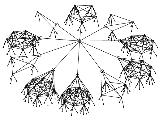
Formally, the problem is given by a triple $(E,T,P)$, where:

• •

  $E$ is a set (set of states);

• •

  $T$ is a nonempty subset of $E$ (target set);

• •

  $P:E\times E\to\mathbb{R}_{+}$ with the following properties:

  • –

    $\forall e\in E$, $\sum P(e,\cdot)=1$;

  • –

    $P^{-1}(0,\infty)\cap(T\times E)\subseteq(T\times T)$.

  $P$ may be identified to the probability transition matrix $P_{i,j}=P((e_{i},e_{j}))$.

As shown in [3], compressing non influent information is equivalent to find a triple $(F,t,P^{*})$ and a map $\pi:E\to F$ s.t.

• •

  $\pi$ is a surjective set function from $E$ to $F$;

• •

  $t=\pi(T)$, $T=\pi^{-1}(t)$;

• •

  the following diagram commutes:

  (2)

  $$\begin{diagram}$$

  where $Id_{E}:E\to E$ is the identity map on $E$, $\mathfrak{P}(E)$ is the power set of $E$ and $\mathbb{P}(e,A)=\sum_{e_{i}\in A}P((e,e_{i}))$.

When the cardinality of $F$ is strictly less than the cardinality of $E$, we have reduced some information: the subsets $\pi^{-1}(f),f\in F$ of $E$ act in the same way for the target problem.

The proof of the optimal solution’s existence was therefore based on the fact that the set of compatible projections $\pi$ has a minimal majorant property. More precisely, if $\pi$ is a projection from $E$ to another set $F$, let $R_{\pi}$ be the equivalence relationship on $E$ defined by $e_{1}\,R_{\pi}\,e_{2}\iff\pi(e_{1})=\pi(e_{2})$. If we define $\widehat{E}:=\{R_{\pi}\colon\pi\text{ satisfies }\ref{eq:diagram}\}$, in [3] it was proved that

Unfortunately, finding a nontrivial $R_{\pi}\in\widehat{E}$ is not a local search. In fact, we may have $P(e_{1},e_{3})\neq P(e_{2},e_{3})$ but $\mathbb{P}(e_{1},\{e_{3},e_{4}\})=\mathbb{P}(e_{2},\{e_{3},e_{4}\})$, which means that $e_{1}\,R_{\pi}\,e_{2}$ may be found if we know that $e_{3}\,R_{\pi}\,e_{4}$. Moreover, it is not difficult to build examples where the only nontrivial element of $\widehat{E}$ corresponds to the optimal nontrivial projection. Therefore, searching for a compressing map $\pi$ appears as a non–polynomial search, in the sense that we have to look at the whole set $\widetilde{E}$ of equivalent relations on $E$. In fact, finding a reducing map means to find $R\in\widetilde{E}$ s.t.

• •

  $\forall e_{i}\in T$ $e_{i}\,R\,e_{j}\iff e_{j}\in T$;

• •

  $\forall\{e_{i},e_{j},e_{k}\}\subseteq E\colon e_{i}Re_{j}$, $\sum_{e_{l}\,R\,e_{k}}P(e_{i},e_{l})=\sum_{e_{l}\,R\,e_{k}}P(e_{j},e_{l})$.

The problem here is to find a polynomial algorithm for reaching the optimal projection of the given Markov chain $(E,P)$ which preserves probabilities of reaching the target set $T$. Moreover, we extend this method to multi–target problems $\mathbf{T}=\{T_{1},\ldots,T_{k}\}$.

As in [3], we act on the set of equivalence relations on a set, but we will focus our attention on $F$ instead of on $E$. For any (finite) set $A$, we denote by $\widetilde{A}$ be the set of all equivalence relations on $A$. Moreover, given an equivalence relation $R\in\widetilde{A}$, we denote by $A/R$ the quotient set of $A$ by $R$. We introduce a partial order $\vDash$ on $\widetilde{A}$. Let $R,S\in\widetilde{A}$. We say that $R\vDash S$ if $a_{1}\,R\,a_{2}$ implies $a_{1}\,S\,a_{2}$ (if you think $A$ as the set of all men and $R$ is “belonging to the same state” while $S$ is “belonging to the same continent”, then $R\vDash S$). The relation $\vDash$ is just set-theoretic inclusion between equivalence relations, since any relation is a subset of $A\times A$. We denote by $|A|$ the cardinality of a set $A$. We state the following trivial lemma without proof.

Let $(E,T,P)$ be a triple, as above and let $\pi:E\to F$ be the optimal projection, (for existence and uniqueness, see [3]). The map $\pi$ is characterized by the equivalence relationship $F_{\pi}$ on $E$: $e_{1}\,F_{\pi}\,e_{2}\iff\pi(e_{1})=\pi(e_{2})$.

Let $\widetilde{F}_{t}$ be the set of all equivalence relations on $F$ such that the target state $t\in F$ is left “alone”: i.e. $R\in\widetilde{F}_{t}$ if $t\,R\,f\iff f=t$.

Note that $\widetilde{F}_{t}\hookrightarrow\widetilde{E}$; more precisely, since $E\mathop{\longrightarrow}\limits^{\pi}F$, we have:

It is obvious that $(\pi,\pi)^{-1}\circ j:\widetilde{F}_{t}\to\mathfrak{P}(E\times E)$ defines an equivalence relationship on $E$. With this inclusion in mind, we can state that $\widetilde{F}_{t}\subseteq\widetilde{E}$:

and hence we refer to $\widetilde{F}_{t}$ both as a class of equivalence relations on $F$ and on $E$. The uniqueness of the optimal solution in [3] states that (4) is well–posed.

We call $I_{F}$ the identity relationship on $F$:

i.e. $I_{F}$ is just $F_{\pi}$ on $\widetilde{F}_{t}$, and let $M_{E}$ be maximal relationship on $\widetilde{F}_{t}$:

Clearly, $M_{E}\in\widetilde{F}_{t}$ and $I_{F}\vDash R\vDash M_{E}$, $\forall R\in\widetilde{F}_{t}$ (i.e., $I_{F}$ and $M_{E}$ are the minimal and maximal relationship on $\widetilde{F}_{t}$). Note that we can compute $M_{E}$ without knowing $F$.

We build now a monotone operator $\mathcal{P}$ on $\widetilde{E}$ (the algorithm’s idea will be to reach $I_{F}$ –unknown– starting from $M_{E}$ –known–).
Let $\mathcal{P}:\widetilde{E}\to\widetilde{E}$ so defined:
for any $R\in\widetilde{E}$, let $r_{1},\ldots,r_{N}$ be the classes of equivalence of $E$ induced by $R$. Define

Now, we focus our attention on the action of $\mathcal{P}$ on $\widetilde{F}_{t}$. First, we prove that $\mathcal{P}:\widetilde{F}_{t}\to\widetilde{F}_{t}$ and then we will show that the unique fixed point of $\mathcal{P}:\widetilde{F}_{t}\to\widetilde{F}_{t}$ is $I_{F}$.

The previous results and those in [3] may be extended to multiple targets problems. More precisely, let ${X}$ be a stationary Markov chain on a at finite set $E$ and let $\mathbf{T}=\{T_{1},\ldots,T_{k}$} be the absorbing disjoint classes of targets. Our interstest is engaged by the computation of the probability of reaching $T_{i}$ by time $\tau$, given the initial distribution $\mu$ on $E$. If $(\Omega,\mathcal{F},Prob)$ is the underlying probability space, we are accordingly interested in

under the assumption that $Prob(\{X_{0}=e\})=\mu(e)$ .

The problem is the following: is there a “minimum” set $F$ such that the problem may be projected to a problem on a Markov chain on $F$, for any initial distribution $\mu$ on $E$?

The answer is trivial, since each target class $T_{i}$ defines its equivalence relationship $I_{F_{i}}$. It is not difficult to show that the required set $F$ is defined by

Let $S_{n}=\sum_{i=1}^{n}Y_{i}$, where $\{Y_{i},i\in\mathbb{N}\}$ is a sequence of i.i.d. bernoulli random variable with $Prob(\{Y_{i}=1\})=1-Prob(\{Y_{i}=0\})=p$. Our interstest is engaged by the computation of the probability of reaching $n$ starting from $0$. Let $E=\{0,1,\ldots,n\}$ be the set of levels we have reached. We have

Since the length of the minimum path for reaching the target state $n$ from different states is different, the problem is irreducible by [3, Proposition 31]. Its Markov complexity is $n+1$.

The problem is similar to the previous one, where

The problem is again irreducible by [3, Proposition 31]. Its Markov complexity is $n+1$.

Let $S_{n}=\sum_{i=1}^{n}(2Y_{i}-1)$, where $\{Y_{i},i\in\mathbb{N}\}$ is a sequence of i.i.d. bernoulli random variable with $Prob(\{Y_{i}=1\})=1-Prob(\{Y_{i}=0\})=p$. Our interstest is engaged by the computation of the probability of reaching $T_{1}=n_{2}$ or $T_{2}=-n_{1}$ (multiple target) starting from $0$. Let $E=\{-n_{2},\ldots,-1,0,1,\ldots,n_{1}\}$ be the set of levels we have reached. We have

This problem is clearly irreducible, since it is for $T_{1}$ (for example). The problem may be reduced if and only if we are interesting in the time of stopping (without knowing who wins, i.e. $\mathbf{T}=T_{1}\cup T_{2}$) and $p=1/2$. In this case, the relevant information is the distance from the nearest border and hence the problem may be half–reduced.

Let $T_{1}=(0,0,0)$, $T_{2}=(1,1,1)$. The following transiction matrix

can be easily reduced on

where $t_{i}=T_{i}$ and $f_{i}=\{e=(e_{1},e_{2},e_{3}):\sum e_{j}=i\}$, i.e. its Markov complexity is $4$. If we are only interesting in the time of stopping (i.e. $\mathbf{T}=T_{1}\cup T_{2}$), the previous problem may be reduced to a geometrical one (Markov complexity equal to $2$). Clearly, this results hold also for random walk on a $d$–dimensional cube.

Let $\Lambda$ be the set of permutations of the $n$ objects. For a fixed permutation $\lambda=(e_{\lambda_{1}},e_{\lambda_{2}},\ldots,e_{\lambda_{n}})\in\Lambda$ we denote by $E^{\lambda^{i}}=\{e_{\lambda_{1}},e_{\lambda_{2}},\ldots,e_{\lambda_{i}}\}$ the set of the first $i$-objects in $\lambda$ (without order!).

Now, let $\mathcal{A}_{\lambda}$ be the set of all the paths that have picked all the $n$ objects with the order given by $\lambda$. In Pattern–Matching Algorithms framework (see [3, Section 3 and Remark 18]), the stopping $\lambda$-rule we consider here is denoted by

and it becomes a target state of an enbedded Markov problem on a graph (see [3, Section 3]). The stopping class for the Coupon Collector’s Problem is accordingly $\mathbf{T}=\cup_{\lambda_{\in}\Lambda}T_{\lambda}$.

It is not difficult to show that the general Coupon Collector’s Problem may be embedded into a Markow network of $2^{n}-1$–nodes (its general Markov hard complexity), where $E=\{\mathbf{T},\{E^{\lambda^{i}}\colon\lambda\in\Lambda,1<i<n\}$, the transition matrix is given by

$\lambda,\zeta\in\Lambda$ and $Prob(\{X^{1}=e_{k}\})=p_{k}$. Note that this matrix is not in general reducible.

If some $p_{i}$ are equal, i.e., when some states act with the same law with respect to the problem, the set $E$ can be projected into a minor one. The easiest case (namely, $p_{i}=1/n$ $\forall i$) is projected into a $n$–state problem:

with $Prob(\{X^{1}=f_{1}\})=1$. Here, $f_{i}=\{E^{\lambda^{i}},\lambda\in\Lambda\}$. The problem is again irreducible by [3, Proposition 31] and its Markov complexity is $n$. In general, when we have $m$ different values of $\{p_{i},i=1,\ldots,n\}$ (namely, $q_{1},\ldots,q_{m}$), if $n_{m}=|k\colon p_{k}=q_{m}|$, then the Markov complexity can be easily proven to be $\prod_{k=1}^{m}(n_{k}+1)-1$.

References

- [1] A. V. Aho, J. E. Hopcroft, and J. D. Ullman. The design and analysis of computer algorithms. Addison-Wesley Publishing Co., Reading, Mass.-London-Amsterdam, 1975. Second printing, Addison-Wesley Series in Computer Science and Information Processing.
- [2] S. Aki and K. Hirano. Sooner and later waiting time problems for runs in Markov dependent bivariate trials. Ann. Inst. Statist. Math., 51(1):17–29, 1999.
- [3] G. Aletti and E. Merzbach. Stopping Markov processes and first path on graphs. J. Eur. Math. Soc. (JEMS), 8(1):49–75, 2006.
- [4] D. L. Antzoulakos and A. N. Philippou. Probability distribution functions of succession quotas in the case of Markov dependent trials. Ann. Inst. Statist. Math., 49(3):531–539, 1997.
- [5] B. C. Arnold, N. Balakrishnan, and H. N. Nagaraja. Records. Wiley Series in Probability and Statistics: Probability and Statistics. John Wiley & Sons Inc., New York, 1998. A Wiley-Interscience Publication.
- [6] R. Cairoli and R. C. Dalang. Sequential stochastic optimization. Wiley Series in Probability and Statistics: Probability and Statistics. John Wiley & Sons Inc., New York, 1996. A Wiley-Interscience Publication.
- [7] M. Ebneshahrashoob and M. Sobel. Sooner and later waiting time problems for Bernoulli trials: frequency and run quotas. Statist. Probab. Lett., 9(1):5–11, 1990.
- [8] M. V. Koutras and V. A. Alexandrou. Sooner waiting time problems in a sequence of trinary trials. J. Appl. Probab., 34(3):593–609, 1997.
- [9] K. Lam and H. C. Yam. Cusum techniques for technical trading in financial markets. Financial Engineering & the Japanese Markets, 4(3):257–274, 1997.
- [10] S. Mac Lane. Categories for the working mathematician, volume 5 of Graduate Texts in Mathematics. Springer-Verlag, New York, second edition, 1998.
- [11] V. T. Stefanov. On some waiting time problems. J. Appl. Probab., 37(3):756–764, 2000.
- [12] V. T. Stefanov and A. G. Pakes. Explicit distributional results in pattern formation. Ann. Appl. Probab., 7(3):666–678, 1997.
- [13] J.-R. Yang and S.-R. Hsiau. On Markov-dependent parking problems. J. Appl. Probab., 41(2):579–586, 2004.