Tug-of-war and the infinity LaplacianThanks: Research of Y.P. and S.S. supported in part by NSF grants DMS-0244479 and DMS-0104073.

We consider a class of zero-sum two-player stochastic games called tug-of-war and use them to prove that every bounded real-valued Lipschitz function $F$ on a subset $Y$ of a length space $X$ admits a unique absolutely minimal (AM) extension to $X$, i.e., a unique Lipschitz extension $u:X\rightarrow{\mathbb{R}}$ for which ${\operatorname{Lip}}_{U}u={\operatorname{Lip}}_{\partial U}u$ for all open $U\subset X\smallsetminus Y$. We present an example that shows this is not generally true when $F$ is merely Lipschitz and positive. (Recall that a metric space $(X,d)$ is a length space if for all $x,y\in X$, the distance $d(x,y)$ is the infimum of the lengths of continuous paths in $X$ that connect $x$ to $y$. Length spaces are more general than geodesic spaces, where the infima need to be achieved.)

When $X$ is the closure of a bounded domain $U\subset{\mathbb{R}}^{n}$ and $Y$ is its boundary, a Lipschitz extension $u$ of $F$ is AM if and only it is infinity harmonic in the interior of $X\smallsetminus Y$, i.e., it is a viscosity solution (defined below) to $\Delta_{\infty}u=0$, where $\Delta_{\infty}$ is the so-called infinity Laplacian

(informally, this is the second derivative of $u$ in the direction of the gradient of $u$). Aronsson proved this equivalence for smooth $u$ in 1967 and Jensen proved the general statement in 1993 [1, 13]. Our analysis of tug-of-war also shows that in this setting $\Delta_{\infty}u=g$ has a unique viscosity solution (extending $F$) when $g:\overline{U}\to{\mathbb{R}}$ is continuous and $\inf g>0$ or $\sup g<0$, but not necessarily when $g$ assumes values of both signs. We note that in the study of the homogenous equation $\Delta_{\infty}u=0$, the normalizing factor $|\nabla u|^{-2}$ in (1.1) is sometimes omitted; however, it is important to include it in the nonhomogenous equation. Observe that with the normalization, $\Delta_{\infty}$ coincides with the ordinary Laplacian $\Delta$ in the one-dimensional case.

Unlike the ordinary Laplacian or the $p$-Laplacian for $p<\infty$, the infinity Laplacian can be defined on any length space with no additional structure (such as a measure or a canonical Markov semigroup)—that is, we will see that viscosity solutions to $\Delta_{\infty}u=g$ are well-defined in this generality. We will establish the above stated uniqueness of solutions $u$ to $\Delta_{\infty}u=g$ in the setting of length spaces.

Originally, we were motivated not by the infinity Laplacian but by random turn Hex [22] and its generalizations, which led us to consider the tug-of-war game. As we later learned, tug-of-war games have been considered by Lazarus, Loeb, Propp and Ullman in [16] (see also [15]).

Tug-of-war on a metric space is very natural and conceivably applicable (like differential game theory) to economic and political modeling.

The intuition provided by thinking of strategies for tug-of-war yields new results even in the classical setting of domains in ${\mathbb{R}}^{n}$. For instance, in Section 4 we show that if $u$ is infinity-harmonic in the unit disk and its boundary values are in $[0,1]$ and supported on a $\delta$-neighborhood of the ternary Cantor set on the unit circle, then $u(0)<\delta^{\beta}$ for some $\beta>0$.

Before precisely stating our main results, we need several definitions.

We consider two-player, zero-sum random-turn games, which are defined by the following parameters: a set $X$ of states of the game, two directed transition graphs $E_{{\rm I}},E_{{\rm II}}$ with vertex set $X$, a nonempty set $Y\subset X$ of terminal states (a.k.a. absorbing states), a terminal payoff function $F:Y\rightarrow{\mathbb{R}}$, a running payoff function $f:X\smallsetminus Y\rightarrow{\mathbb{R}}$, and an initial state $x_{0}\in X$.

Game play is as follows: a token is initially placed at position $x_{0}$. At the $k^{\text{th}}$ step of the game, a fair coin is tossed, and the player who wins the toss may move the token to any $x_{k}$ for which $(x_{k-1},x_{k})$ is a directed edge in her transition graph. The game ends the first time $x_{k}\in Y$, and player I’s payoff is $F(x_{k})+\sum_{i=0}^{k-1}f(x_{i})$. Player I seeks to maximize this payoff, and since the game is zero-sum, player II seeks to minimize it.

We will use the term tug-of-war (on the graph with edges $E$) to describe the game in which $E:=E_{\rm I}=E_{\rm II}$ (i.e., players have identical move options) and $E$ is undirected (i.e., all moves are reversible). Generally, our results pertain only to the undirected setting. Occasionally, we will also mention some counterexamples showing that the corresponding results do not hold in the directed case.

In the most conventional version of tug-of-war on a graph, $Y$ is a union of “target sets” $Y^{\rm I}$ and $Y^{{\rm II}}$, there is no running payoff ($f=0$) and $F$ is identically $1$ on $Y^{\rm I}$, identically $0$ on $Y^{{\rm II}}$. Players then try to “tug” the game token to their respective targets (and away from their opponent’s targets) and the game ends when a target is reached.

A strategy for a player is a way of choosing the player’s next move as a function of all previously played moves and all previous coin tosses. It is a map from the set of partially played games to moves (or in the case of a random strategy, a probability distribution on moves). Normally, one would think of a good strategy as being Markovian, i.e., as a map from the current state to the next move, but it is useful to allow more general strategies that take into account the history.

Given two strategies $\mathcal{S}_{{\rm I}},\mathcal{S}_{{\rm II}}$, let $F_{-}(\mathcal{S}_{{\rm I}},\mathcal{S}_{{\rm II}})$ and $F_{+}(\mathcal{S}_{{\rm I}},\mathcal{S}_{{\rm II}})$ be the expected total payoff (including the running payoffs received) at the termination of the game — if the game terminates with probability one and this expectation exists in $[-\infty,\infty]$; otherwise, let $F_{-}(\mathcal{S}_{{\rm I}},\mathcal{S}_{{\rm II}})=-\infty$ and $F_{+}(\mathcal{S}_{{\rm I}},\mathcal{S}_{{\rm II}})=+\infty$.

The value of the game for player Iis defined as $\sup_{\mathcal{S}_{\rm I}}\inf_{\mathcal{S}_{\rm II}}F_{-}(\mathcal{S}_{\rm I},\mathcal{S}_{\rm II})$. The value for player IIis $\inf_{\mathcal{S}_{{\rm II}}}\sup_{\mathcal{S}_{{\rm I}}}F_{+}(\mathcal{S}_{{\rm I}},\mathcal{S}_{{\rm II}})$. We use the expressions $u_{{\rm I}}(x)$ and $u_{{\rm II}}(x)$ to denote the values for players I and II, respectively, as a function of the starting state $x$ of the game.

Note that if player I cannot force the game to end almost surely, then $u_{{\rm I}}=-\infty$, and if player II cannot force the game to end almost surely, then $u_{{\rm II}}=\infty$. Clearly, $u_{{\rm I}}(x)\leq u_{{\rm II}}(x)$. When $u_{{\rm I}}(x)=u_{{\rm II}}(x)$, we say that the game has a value, given by $u(x):=u_{{\rm I}}(x)=u_{{\rm II}}(x)$.

Our definition of value for player I penalizes player I severely for not forcing the game to terminate with probability one, awarding $-\infty$ in this case.

(As an alternative definition, one could define $F_{-}$, and hence player I’s value, by assigning payoffs to all of the non-terminating sequences $x_{0},x_{1},x_{2},\ldots$. If the payoff function for the non-terminating games is a zero-sum Borel-measurable function of the infinite sequence, then player I’s value is equal to player II’s value in great generality [17]; see also [20] for more on stochastic games. The existence of a value by our strong definition implies the existence and equality of the values defined by these alternative definitions.)

Considering the two possibilities for the first coin toss yields the following lemma, a variant of which appears in [16].

When $E=E_{1}=E_{2}$, the operator

is called the (discrete) infinity Laplacian. A function $u$ is infinity harmonic if (1.2) holds and $f(x)=0$ at all non-terminal $x\in X\smallsetminus Y$. When $u$ is finite, this is equivalent to $\Delta_{\infty}u=0$. However, it will be convenient to adopt the convention that $u$ is infinity harmonic at $x$ if $u(x)=+\infty$ (resp. $-\infty$) and the right hand side in (1.2) is also $+\infty$ (resp. $-\infty$). Similarly, it will be convenient to say “$u$ is a solution to $\Delta_{\infty}u=-2\,f$” at $x$ if $u(x)=+\infty$ (resp. $-\infty$) and the right hand side in (1.2) is also $+\infty$ (resp. $-\infty$).

In a tug-of-war game, it is natural to guess that the value $u=u_{{\rm I}}=u_{{\rm II}}$ exists and is the unique solution to

and also that (at least when $E$ is locally finite) player I’s optimal strategy will be to always move to the vertex that maximizes $u(x)$, and player II’s optimal strategy will be to always move to the vertex that minimizes $u(x)$. This is easy to prove when $E$ is undirected and finite and $f$ is everywhere positive or everywhere negative. Subtleties arise in more general cases ($X$ infinite, $E$ directed, $F$ unbounded, $f$ having values of both signs, etc.)

Our first theorem addresses the question of the existence of a value.

Counterexamples exist when any one of the three criteria is removed. In Section 5 (a section devoted to counterexamples) we give an example of a tug-of-war game without a value, where $E$ is undirected, $F=0$, and the running payoff satisfies $f>0$ but $\inf f=0$.

The case where $f=0$, $F$ is bounded, and $(X,E)$ is locally finite was proved earlier in [15]. That paper discusses an (essentially non-random) game in which the two players bid for the right to choose the next move. That game, called the Richman game, has the same value as tug-of-war with $f=0$ where $F$ takes the values $0$ and $1$. Additionally, a simple and efficient algorithm for calculating the value when $f=0$ and $(X,E)$ is finite is presented there.

Consider now the special case that $(X,d)$ is a metric space, $Y\subset X$, and Lipschitz functions $F:Y\rightarrow{\mathbb{R}}$ and $f:X\smallsetminus Y\rightarrow{\mathbb{R}}$ are given. Let $E_{\varepsilon}$ be the edge-set in which $x\sim y$ if and only if $d(x,y)<\varepsilon$ and let $u^{\varepsilon}$ be the value (if it exists) of the game played on $E_{\varepsilon}$ with terminal payoff $F$ and running payoff normalized to be $\varepsilon^{2}f$.

In other words, $u^{\varepsilon}(x)$ is the value of the following two-player zero-sum game, called $\varepsilon$-tug-of-war: fix $x_{0}=x\in X\smallsetminus Y$. At the $k^{\text{th}}$ turn, the players toss a coin and the winner chooses an $x_{k}$ with $d(x_{k},x_{k-1})<\varepsilon$. The game ends when $x_{k}\in Y$, and player I’s payoff is $F(x_{k})+\varepsilon^{2}\sum_{i=0}^{k-1}f(x_{i})$.

When the limit $u:=\lim_{\varepsilon\rightarrow 0}u^{\varepsilon}$ exists pointwise, we call $u$ the continuum value (or just “value”) of the quintuple $(X,d,Y,F,f)$. We define the continuum value for player I(or II) analogously.

The reader may wonder why we have chosen not to put an edge in $E_{\varepsilon}$ between $x$ and $y$ when $d(x,y)=\varepsilon$ exactly. This choice has some technical implications. Specifically, we will compare the $\varepsilon$-game with the $2\,\varepsilon$-game. If $x,z$ are such that $d(x,z)\leq 2\,\varepsilon$, then in a length-space it does not follow that there is a $y$ such that $d(x,y)\leq\varepsilon$ and $d(y,z)\leq\varepsilon$. However, it does follow if you replace the weak inequalities with strong inequalities throughout.

We prove the following:

The above condition that $F:Y\rightarrow{\mathbb{R}}$ extends to a uniformly continuous function on $X$ is equivalent to having $F$ uniformly continuous on $Y$ and “Lipschitz on large scales,” as we prove in Lemma 3.9 below.

We will see in Section 5.1 that this fails in general when $f>0$ but $\inf f=0$. When $f$ assumes values of both signs, it fails even when $X$ is a closed disk in ${\mathbb{R}}^{2}$, $Y$ is its boundary and $F=0$. In Section 5.3 we show by means of an example that in such circumstances it may happen that $u_{\rm I}^{\varepsilon}\neq u_{\rm II}^{\varepsilon}$ and moreover, $\liminf_{\varepsilon\searrow 0}\|u_{\rm I}^{\varepsilon}-u_{\rm II}^{\varepsilon}\|_{\infty}>0$.

Given a metric space $(X,d)$, a subset $Y\subset X$ and a function $u:X\rightarrow{\mathbb{R}}$, we write ${\operatorname{Lip}}_{Y}u=\sup_{x,y\in Y}|u(y)-u(x)|/d(x,y)$ and ${\operatorname{Lip}}\,u={\operatorname{Lip}}_{X}u$. Thus $u$ is Lipschitz iff ${\operatorname{Lip}}\,u<\infty$. Given $F:Y\to{\mathbb{R}}$, we say that $u:X\rightarrow{\mathbb{R}}$ is a minimal extension of $F$ if ${\operatorname{Lip}}_{X}u={\operatorname{Lip}}_{Y}F$ and $u(y)=F(y)$ for all $y\in Y$.

It is well known that for any metric space $X$, any Lipschitz $F$ on a subset $Y$ of $X$ admits a minimal extension. The largest and smallest minimal extensions (introduced by McShane [18] and Whitney [24] in the 1930’s) are respectively

We say $u$ is an absolutely minimal (AM) extension of $F$ if ${\operatorname{Lip}}\,u<\infty$ and ${\operatorname{Lip}}_{U}u={\operatorname{Lip}}_{\partial U}u$ for every open set $U\subset X\smallsetminus Y$. We say that $u$ is AM on $U$ if it is defined on $\overline{U}$ and is an AM extension of its restriction to $\partial U$. AM extensions were first introduced by Aronsson in 1967 [1] and have applications in engineering and image processing (see [4] for a recent survey).

We prove the following:

We present in the counterexample section, Section 5, an example in which $F$ is Lipschitz, non-negative, and unbounded, and although the continuum value is an AM extension, it is not the only AM extension.

Prior to our work, the existence of AM extensions in the above settings was known only for separable length spaces [14] (see also [19]). The uniqueness in Theorem 1.4 was known only in the case that $X$ is the closure of a bounded domain $U\subset{\mathbb{R}}^{n}$ and $Y=\partial U$. (To deduce this case from Theorem 1.4, one needs to replace $X$ by the smallest closed ball containing $\overline{U}$, say.) Three uniqueness proofs in this setting have been published, by Jensen [13], by Barles and Busca [6], and by Aronsson, Crandall, and Juutinen [4]. The third proof generalizes from the Euclidean norm to uniformly convex norms.

Our proof applies to more general spaces because it invokes no outside theorems from analysis (which assume existence of a local Euclidean geometry, a measure, a notion of twice differentiability, etc.), and relies only on the structure of $X$ as a length space.

As noted in [4], AM extensions do not generally exist on metric spaces that are not length spaces. (For example, if $X$ is the $L$-shaped region $\{0\}\times[0,1]\cup[0,1]\times\{0\}\subset{\mathbb{R}}^{2}$, with the Euclidean metric, and $Y=\{(0,1),(1,0)\}$, then no non-constant $F:Y\rightarrow{\mathbb{R}}$ has an AM extension. Indeed, suppose that $u:X\rightarrow{\mathbb{R}}$ is an AM extension of $F:Y\rightarrow{\mathbb{R}}$. Let $a:=u(0,0)$, $b:=u(0,1)$ and $c:=u(1,0)$. Then, considering $U=\{0\}\times(0,1)$, it follows that $u(0,s)=a+s\,(b-a)$. Likewise, $u(s,0)=a+s\,(c-a)$. Now taking $U_{\epsilon}:=\{0\}\times[0,1)\cup[0,\epsilon)\times\{0\}$, we see that $\lim_{\varepsilon\searrow 0}{\operatorname{Lip}}_{U_{\varepsilon}}u=|b-a|$. Hence $|c-a|\leq|b-a|$. By symmetry, $|c-a|=|b-a|$. Since $F$ is assumed to be nonconstant, $b\neq c$, and hence $c-a=a-b$. Then $\bigl|u(0,s)-u(s,0)\bigr|/\bigl(\sqrt{2}s\bigr)=\sqrt{2}\,|b-a|$, which contradicts $\lim_{\varepsilon\searrow 0}{\operatorname{Lip}}_{U_{\varepsilon}}u=|b-a|$.)

One property that makes length spaces special is that the Lipschitz norm is determined locally. More precisely, if $W\subset X$ is closed, then either ${\operatorname{Lip}}_{W}u={\operatorname{Lip}}_{\partial W}u$ or for every $\delta>0$

The definition of AM is inspired by the notion that if $u$ is the “tautest possible” Lipschitz extension of $F$, it should be tautest possible on any open $V\subset X\smallsetminus Y$, given the values of $u$ on $\partial V$ and ignoring the rest of the metric space. Without locality, the rest of the metric space cannot be ignored (since long-distance effects may change the global Lipschitz constant), and the definition of AM is less natural. Another important property of length spaces is that the graph distance metric on $E_{\varepsilon}$ scaled by $\varepsilon$ approximates the original metric, namely, it is within $\varepsilon$ of $d(\cdot,\cdot)$.

The continuum version of the infinity Laplacian is defined for $C^{2}$ functions $u$ on domains $U\subset{\mathbb{R}}^{n}$ by

This is the same as $\eta^{T}H\eta$, where $H$ is the Hessian of $u$ and $\eta=\nabla u/|\nabla u|$. Informally, $\Delta_{\infty}u$ is the second derivative of $u$ in the direction of the gradient of $u$. If $\nabla u(x)=0$ then, $\Delta_{\infty}u(x)$ is undefined; however, we adopt the convention that if the second derivative of $u(x)$ happens to be the same in every direction (i.e, the matrix $\{u_{x_{i}x_{j}}\}$ is $\lambda$ times the identity), then $\Delta_{\infty}u(x)=\lambda$, which is the second derivative in any direction. (As mentioned above, some texts on infinity harmonic functions define $\Delta_{\infty}$ without the normalizing factor $|\nabla u|^{-2}$. When discussing viscosity solutions to $\Delta_{\infty}u=0$, the two definitions are equivalent. The fact that the normalized version is sometimes undefined when $\nabla u=0$ turns out not to matter because it is always well-defined at $x$ when $\varphi$ is a cone function, i.e., it has the form $a|x-z|+b$ for $a,b\in{\mathbb{R}}$ and $z\in{\mathbb{R}}^{n}$ with $z\neq x$, and viscosity solutions can be defined via comparison with cones, see Section 1.6.) As in the discrete setting, $u$ is infinity harmonic if $\Delta_{\infty}u=0$.

While discrete infinity-harmonic functions are a recent concept, introduced in finite-difference schemes for approximating continuous infinity harmonic functions [21], related notions of value for stochastic games are of course much older. The continuous infinity Laplacian appeared first in the work of Aronsson [1] and has been very thoroughly studied [4]. Key motivations for studying this operator are the following:

1. (1)

   AM extensions: Aronsson proved that $C^{2}$ extensions $u$ on domains $U\subset{\mathbb{R}}^{n}$ (of functions $F$ on $\partial U$) are infinity harmonic if and only if they are AM.

2. (2)

   $p$-harmonic functions: As noted by Aronsson [1], the infinity Laplacian is the formal limit, as $p\rightarrow\infty$ of the (properly normalized) $p$-Laplacians. Recall that $p$-harmonic functions, i.e. minimizers $u$ of $\int|\nabla u(x)|^{p}\,dx$ subject to boundary conditions, solve the Euler-Lagrange equation

   $$\nabla\cdot(|\nabla u|^{p-2}\nabla u)=0,$$

   which can be rewritten

   $$|\nabla u|^{p-2}\left(\Delta u+(p-2)\Delta_{\infty}u\right)=0,$$

   where $\Delta$ is the ordinary Laplacian. Dividing by $|\nabla u|^{p-2}$, we see that (at least when $|\nabla u|\neq 0$) $p$-harmonic functions satisfy $\Delta_{p}u=0$, where $\Delta_{p}:=\Delta_{\infty}+(p-2)^{-1}\Delta$; the second term vanishes in the large $p$ limit. It is not too hard to see that as $p$ tends to infinity, the Lipschitz norm of any limit of the $p$-harmonic functions extending $F$ will be ${\operatorname{Lip}}_{\partial U}F$; so it is natural to guess (and was proved in [7]) that as $p$ tends to infinity the $p$-harmonic extensions of $F$ converge to a limit that is both absolutely minimal and a viscosity solution to $\Delta_{\infty}u=0$.

In the above setting, Aronsson also proved that there always exists an AM extension, and that in the planar case $U\subset{\mathbb{R}}^{2}$, there exists at most one $C^{2}$ infinity harmonic extension; however $C^{2}$ infinity harmonic extensions do not always exist [2].

To define the infinity Laplacian in the non-$C^{2}$ setting requires us to consider weak solutions; the right notion here is that of viscosity solution, as introduced by Crandall and Lions (1983) [11]. Start by observing that if $u$ and $v$ are $C^{2}$ functions, $u(x)=v(x)$, and $v\geq u$ in a neighborhood of $x$, then $v-u$ has a local minimum at $x$, whence $\Delta_{\infty}v(x)\geq\Delta_{\infty}u(x)$ (if both sides of this inequality are defined). This comparison principle (which has analogs for more general degenerate elliptic PDEs [5]) suggests that if $u$ is not $C^{2}$, in order to define $\Delta_{\infty}u(x)$ we want to compare it to $C^{2}$ functions $\varphi$ for which $\Delta_{\infty}\varphi(x)$ is defined. Let $S(x)$ be the set of real valued functions $\varphi$ defined and $C^{2}$ in a neighborhood of $x$ for which $\Delta_{\infty}\varphi(x)$ has been defined; that is, either $\nabla\varphi(x)\neq 0$ or $\nabla\varphi(x)=0$ and the limit $\Delta_{\infty}\varphi(x):=\lim_{x^{\prime}\to x}2\,\frac{\varphi(x^{\prime})-\varphi(x)}{|x^{\prime}-x|^{2}}$ exists.

Similarly, let

and call $u$ a viscosity supersolution of $\Delta_{\infty}(\cdot)=g$ iff $\Delta_{\infty}^{-}u\leq g$ in $X$.

Finally, $u$ is a viscosity solution of $\Delta_{\infty}(\cdot)=g$ if $\Delta_{\infty}^{-}u\leq g\leq\Delta_{\infty}^{+}u$ in $X$ (i.e., $u$ is both a supersolution and a subsolution).

Here is a little caveat. At present, we do not know how to show that $\Delta_{\infty}u=g$ in the viscosity sense determines $g$. For example, if $u$ is Lipschitz, $g_{1}$ and $g_{2}$ are continuous, and $\Delta_{\infty}u=g_{j}$ holds for $j=1,2$ (in the viscosity sense), how does one prove that $g_{1}=g_{2}$?

The following result of Jensen (alluded to above) is now well known [1, 13, 4]: If $X$ is a domain in ${\mathbb{R}}^{n}$ and $u:X\rightarrow{\mathbb{R}}$ continuous, then ${\operatorname{Lip}}_{U}u={\operatorname{Lip}}_{\partial U}u<\infty$ for every bounded open set $U\subset\overline{U}\subset X$ (i.e., $u$ is AM) if and only if $u$ is a viscosity solution to $\Delta_{\infty}u=0$ in $X$.

Let $A\subset Y\subset X$, where $A$ is closed, $Y\neq\emptyset$ and $X$ is a length space. If $x\in X$, one can define the $\infty$-harmonic measure of $A$ from $x$ as the infimum of $u(x)$ over all functions $u:X\to[0,\infty)$ that are Lipschitz on $X$, AM in $X\smallsetminus Y$ and satisfy $u\geq 1$ on $A$. This quantity will be denoted by $\omega_{\infty}(A)=\omega^{(x,Y,X)}_{\infty}(A)$. In Section 4 we prove

Numerical calculations [21] had suggested that in the setting of the theorem $\omega_{\infty}(A_{\delta})$ tends to $0$ as $\delta\to 0$, but this was only recently proved [12], and the proof did not yield any quantitative information on the rate of decay. In contrast to our other theorems in the paper, the proof of this theorem does not use tug-of-war. The primary tool is comparison with a specific AM function in ${\mathbb{R}}^{2}\smallsetminus\{0\}$ with decay $r^{-1/3}$ discovered by Aronsson [3].

To motivate the next definition, observe that for continuous functions $u:{\mathbb{R}}\to{\mathbb{R}}$, the inequality $\Delta_{\infty}^{+}u\geq 0$ reduces to convexity. The definition of convexity requiring a function to lie below its chords has an analog, comparison with cones, which characterizes infinity-harmonic functions. Call the function $\varphi(y)=b\,|y-z|+c$ a cone based at $z\in{\mathbb{R}}^{n}$. For an open $U\subset{\mathbb{R}}^{n}$, say that a continuous $u:U\to{\mathbb{R}}$ satisfies comparison with cones from above on $U$ if for every open $W\subset\overline{W}\subset U$ for every $z\in{\mathbb{R}}^{n}\smallsetminus W$, and for every cone $\varphi$ based at $z$ such that the inequality $u\leq\varphi$ holds on $\partial W$, the same inequality is valid throughout $W$. Comparison with cones from below is defined similarly using the inequality $u\geq\varphi$.

Jensen [13] proved that viscosity solutions to $\Delta_{\infty}u=0$ for domains in ${\mathbb{R}}^{n}$ satisfy comparison with cones (from above and below), and Crandall, Evans, and Gariepy [9] proved that a function on ${\mathbb{R}}^{n}$ is absolutely minimal in a bounded domain $U$ if and only if it satisfies comparison with cones in $U$.

Champion and De Pascale [8] adapted this definition to length spaces, where cones are replaced by functions of the form $\varphi(x)=b\,d(x,z)+c$ where $b>0$. Their precise definition is as follows. Let $U$ be an open subset of a length-space $X$ and let $u:\overline{U}\to{\mathbb{R}}$ be continuous. Then $u$ is said to satisfy comparison with distance functions from above on $U$ if for every open $W\subset U$, for every $z\in X\smallsetminus W$ for every $b\geq 0$ and for every $c\in{\mathbb{R}}$ if $u(x)\leq b\,d(x,z)+c$ holds on $\partial W$, then it also holds in $W$. The function $u$ is said to satisfy comparison with distance functions from below if $-u$ satisfies comparison with distance functions from above. Finally, $u$ satisfies comparison with distance functions if it satisfies comparison with distance functions from above and from below.

The following result from [8] will be used in the proof of Theorem 1.4:

To study the inhomogenous equation $\Delta_{\infty}u=g$, because $u$ will in general have non-zero second derivative (in its gradient direction), it is natural to extend these definitions to comparison with functions that have a quadratic term.

The following theorem is proved in Section 6.

This equivalence motivates the study of functions satisfying quadratic comparison. Note that satisfying $\Delta_{\infty}u(x)=g(x)$ in the viscosity sense depends only on the local behavior of $u$ near $x$. We may use Theorem 1.7 to extend the definition of $\Delta_{\infty}$ to length spaces; saying that $\Delta_{\infty}u=g$ on an open subset $U$ of a length space if and only if every $x\in U$ has a neighborhood $V\subset U$ on which $u$ satisfies $g$-quadratic comparison. We warn the reader, however, that even for length spaces $X$ contained within ${\mathbb{R}}$, there can be solutions to $\Delta_{\infty}u=0$ that do not satisfy comparison with distance functions, (or $0$-quadratic comparison, for that matter): for example, $X=U=(0,1)$ and $u(x)=x$. The point here is that when we take $V\subset(0,1)$ and compare $u$ with some function $\varphi$ on $\partial V$, the “appropriate” notion of the boundary $\partial V$ is the boundary in ${\mathbb{R}}$, not in $X$.

The continuum value of the tug-of-war game sometimes gives a construction of a function satisfying $g$-quadratic comparison. We prove:

Putting these last two theorems together, we obtain

It is easy to verify that $F$ indeed satisfies the assumptions in Theorem 1.8. In order to deduce the Corollary, we may take the length space $X$ as a ball in ${\mathbb{R}}^{n}$ which contains $U$ and extend $F$ to $X\smallsetminus U$, say. Alternatively, we may consider $U$ with its intrinsic metric and lift $F$ to the completion of $U$.

We present in Section 5 an example showing that the corollary may fail if $f$ is permitted to take values of both signs. Specifically, the example describes two functions $u_{1},u_{2}$ defined in the closed unit disk in ${\mathbb{R}}^{2}$ and having boundary values identically zero on the unit circle such that with some Lipschitz function $g$ we have $\Delta_{\infty}u_{j}=g$ for $j=1,2$ (in the viscosity sense), while $u_{1}\neq u_{2}$.

The plan of the paper is as follows. Section 2 discusses the discrete tug-of-war on graphs and proves Theorem 1.2, and Section 3 deals with tug-of-war on length spaces and proves Theorems 1.3, 1.4 and 1.8. Section 4 is devoted to estimates of $\infty$-harmonic measure. In Section 5, we present a few counter-examples showing that some of the assumptions in the theorems we prove are necessary. Section 6 is devoted to the proof of Theorem 1.7. Section 7 presents some heuristic argument describing what the limiting trajectories of some $\epsilon$-tug-of-war games on domains in ${\mathbb{R}}^{n}$ may look like and states a question regarding the length of the game. We conclude with additional open problems in Section 8.

In this section, we will generally assume $E=E_{{\rm I}}=E_{{\rm II}}$ is undirected and connected and $f=0$.

Though we will not use this fact, it is interesting to point out that in the case where $E$ is finite, there is a simple algorithm from [15] which calculates the value $u$ of the game and proceeds as follows. Assuming the value $u(v)$ is already calculated at some set $V^{\prime}\supset Y$ of vertices, find a path $v_{0},v_{1},\dots,v_{k}$, $k>1$, with interior vertices $v_{1},\dots,v_{k-1}\in X\smallsetminus V^{\prime}$ and endpoints $v_{0},v_{k}\in V^{\prime}$ which maximizes $\bigl(u(v_{k})-u(v_{0})\bigr)/k$ and set $u(v_{i})=u(v_{0})+i\,\bigl(u(v_{k})-u(v_{0})\bigr)/k$ for $i=1,2,\dots,k-1$. Repeat as long as $V^{\prime}\neq X$.

Recall that $u_{\rm I}$ is the value function for player I.

Similarly, if $F$ is bounded above on $Y$, then $u_{\rm II}$ is the largest $\infty$-harmonic function bounded above on $X$ that extends $F$.

Now, we prove the first part of Theorem 1.2: When the graph $(X,E)$ is locally finite and $Y$ is finite, this was proven in [15, Thm. 17].

Before we prove this, we discuss several counterexamples that occur when the conditions of the theorem are not met. First, this theorem can fail if $E$ is directed. A trivial counterexample is when $X$ is finite and there is no directed path from the initial state to $Y$.

If $X$ is infinite and $E$ is directed, then there are counterexamples to Theorem 2.2 even when every vertex lies on a directed path towards a terminal state. For example, suppose $X={\mathbb{N}}$ and $Y=\{0\}$, with $F(0)=0$. If $E$ consists of directed edges of the form $(n,n-1)$ and $(n,n+2)$, then II may play so that with positive probability the game never terminates, and hence the value for player I is by definition $-\infty$.

Even in the undirected case, a game may not have a value if $F$ is not bounded either from above or below. The reader may check that if $X$ is the integer lattice ${\mathbb{Z}}^{2}$ and the terminal states are the $x$-axis with $F((x,0))=x$, then the players’ value functions are given by $u_{{\rm I}}((x,y))=x-|y|$ and $u_{{\rm II}}((x,y))=x+|y|$. (Roughly speaking, this is because, in order to force the game to end in a finite amount of time, player I has to “give up” $|y|$ opportunities to move to the right.) Observe also that in this case any linear function which agrees with $F$ on the $x$-axis is $\infty$-harmonic.

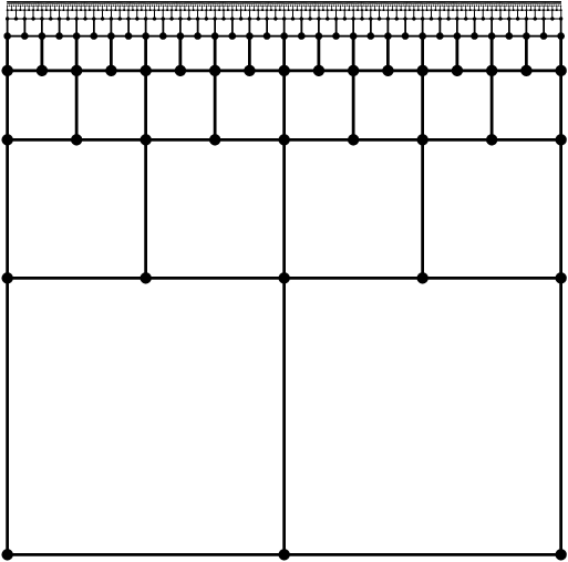
As a final remark before proving this theorem, let us consider the obvious strategy for the two players, namely for player I to always maximize $u$ on her turn and for II to always minimize $u$ on her turn. Even when $E$ is (undirected and) locally finite and the payoff function satisfies $0\leq F\leq 1$, these obvious strategies need not be optimal. Consider, e.g., the game shown in Figure 1, where $X\subset{\mathbb{R}}^{2}$ is given by $X=\bigl\{v(k,j):j=1,2,\dots;k=0,1,\dots,2^{j}\bigr\}$, $v(k,j)=(2^{-j}k,1-2^{-j+1})$, and $E$ consists of edges of the form $\{v(k,j),v(k+1,j)\}$ and $\{v(k,j),v(2k,j+1)\}$. The terminal states are on the left and right edges of the square, and the payoff is $1$ on the left and $0$ on the right. Clearly the function $u(v(k,j))=1-k/2^{j}$ (the Euclidean distance from the right edge of the square) is infinity-harmonic, and by Corollary 2.3 below, we have $u_{\rm I}=u=u_{\rm II}$. The obvious strategy for player I is to always move left, and for II it is to always move right. Suppose however that player I always pulls left and player II always pulls up. It is easy to check that the probability that the game ever terminates when starting from $v(k,j)$ is at most $2/(k+2)$ (this function is a supermartingale under the corresponding Markov chain). Therefore the game continues forever with positive probability, resulting in a payoff of $-\infty$ to player I. Thus, a near-optimal strategy for player I must be able to force the game to end, and must be prepared to make moves which do not maximize $u$. (This is a well known phenomenon, not particular to tug-of-war.)

References

- [1] Gunnar Aronsson, Extension of functions satisfying Lipschitz conditions, Ark. Mat. 6 (1967), 551–561. MR0217665 (36 #754)
- [2] by same author, On the partial differential equation , Ark. Mat. 7 (1968), 395–425. MR0237962 (38 #6239)
- [3] by same author, Construction of singular solutions to the -harmonic equation and its limit equation for , Manuscripta Math. 56 (1986), no. 2, 135–158. MR850366 (87j:35070)
- [4] Gunnar Aronsson, Michael G. Crandall, and Petri Juutinen, A tour of the theory of absolutely minimizing functions, Bull. Amer. Math. Soc. (N.S.) 41 (2004), no. 4, 439–505 (electronic). MR2083637 (2005k:35159)
- [5] M. Bardi, M. G. Crandall, L. C. Evans, H. M. Soner, and P. E. Souganidis, Viscosity solutions and applications, Lecture Notes in Mathematics, vol. 1660, Springer-Verlag, Berlin, 1997, Lectures given at the 2nd C.I.M.E. Session held in Montecatini Terme, June 12–20, 1995, Edited by I. Capuzzo Dolcetta and P. L. Lions, Fondazione C.I.M.E.. [C.I.M.E. Foundation]. MR1462698 (98b:35005)
- [6] G. Barles and Jérôme Busca, Existence and comparison results for fully nonlinear degenerate elliptic equations without zeroth-order term, Comm. Partial Differential Equations 26 (2001), no. 11-12, 2323–2337. MR1876420 (2002k:35078)
- [7] T. Bhattacharya, E. DiBenedetto, and J. Manfredi, Limits as of and related extremal problems, Rend. Sem. Mat. Univ. Politec. Torino 1989 (1991), no. Special issue on topics in nonlinear PDEs, 15–68. MR1155453 (93a:35049)
- [8] Thierry Champion and Luigi De Pascale, Principles of comparison with distance functions for absolute minimizers, J. Convex Anal. 14 (2007), no. 3, 515–541. MR2341302
- [9] M. G. Crandall, L. C. Evans, and R. F. Gariepy, Optimal Lipschitz extensions and the infinity Laplacian, Calc. Var. Partial Differential Equations 13 (2001), no. 2, 123–139. MR1861094 (2002h:49048)
- [10] Michael G. Crandall and L. C. Evans, A remark on infinity harmonic functions, Proceedings of the USA-Chile Workshop on Nonlinear Analysis (Viña del Mar-Valparaiso, 2000) (San Marcos, TX), Electron. J. Differ. Equ. Conf., vol. 6, Southwest Texas State Univ., 2001, pp. 123–129 (electronic). MR1804769 (2001j:35076)
- [11] Michael G. Crandall and Pierre-Louis Lions, Viscosity solutions of Hamilton-Jacobi equations, Trans. Amer. Math. Soc. 277 (1983), no. 1, 1–42. MR690039 (85g:35029)
- [12] Lawrence C. Evans and Yifeng Yu, Various properties of solutions of the infinity-Laplacian equation, Comm. Partial Differential Equations 30 (2005), no. 7-9, 1401–1428. MR2180310 (2006g:35062)
- [13] Robert Jensen, Uniqueness of Lipschitz extensions: minimizing the sup norm of the gradient, Arch. Rational Mech. Anal. 123 (1993), no. 1, 51–74. MR1218686 (94g:35063)
- [14] Petri Juutinen, Absolutely minimizing Lipschitz extensions on a metric space, Ann. Acad. Sci. Fenn. Math. 27 (2002), no. 1, 57–67. MR1884349 (2002m:54020)
- [15] Andrew J. Lazarus, Daniel E. Loeb, James G. Propp, Walter R. Stromquist, and Daniel H. Ullman, Combinatorial games under auction play, Games Econom. Behav. 27 (1999), no. 2, 229–264. MR1685133 (2001f:91023)
- [16] Andrew J. Lazarus, Daniel E. Loeb, James G. Propp, and Daniel Ullman, Richman games, Games of No Chance (Richard J. Nowakowski, ed.), MSRI Publications, vol. 29, Cambridge Univ. Press, Cambridge, 1996, pp. 439–449. MR1427981 (97j:90101)
- [17] Donald A. Martin, The determinacy of Blackwell games, J. Symbolic Logic 63 (1998), no. 4, 1565–1581. MR1665779 (2000d:03118)
- [18] E. J. McShane, Extension of range of functions, Bull. Amer. Math. Soc. 40 (1934), no. 12, 837–842.
- [19] V. A. Mil′man, Absolutely minimal extensions of functions on metric spaces, Mat. Sb. 190 (1999), no. 6, 83–110. MR1719573 (2000j:41041)
- [20] Abraham Neyman and Sylvain Sorin (eds.), Stochastic games and applications, NATO Science Series C: Mathematical and Physical Sciences, vol. 570, Dordrecht, Kluwer Academic Publishers, 2003. MR2032421 (2004h:91004)
- [21] Adam M. Oberman, A convergent difference scheme for the infinity Laplacian: construction of absolutely minimizing Lipschitz extensions, Math. Comp. 74 (2005), no. 251, 1217–1230 (electronic). MR2137000 (2006h:65165)
- [22] Yuval Peres, Oded Schramm, Scott Sheffield, and David B. Wilson, Random-turn Hex and other selection games, Amer. Math. Monthly 114 (2007), no. 5, 373–387. MR2309980 (2008a:91039)
- [23] Ovidiu Savin, regularity for infinity harmonic functions in two dimensions, Arch. Ration. Mech. Anal. 176 (2005), no. 3, 351–361. MR2185662 (2006i:35108)
- [24] Hassler Whitney, Analytic extensions of differentiable functions defined in closed sets, Trans. Amer. Math. Soc. 36 (1934), no. 1, 63–89. MR1501735
- [25] Yifeng Yu, Uniqueness of values of Aronsson operators and applications to “tug-of-war” game theory, 2007, http://www.ma.utexas.edu/~yifengyu/uofa2d.pdf.