1Introduction

\NONUMBIB

\SPECFNSYMBOL

12\AOSMAKETITLE

\AOSyr

2006 \AOSvol00 \AOSno00 \AOSpp000–000 \AOSReceivedReceived \AOSAMSPrimary 62H20; secondary 62E99 \AOSKeywordscorrelation, covariance, test of independence, spectral decomposition, eigenvalues, eigenfunctions, Hilbert-Schmidt operator, Fréchet bounds, contingency tables, phi-square, canonical correlation, Cramér-von Mises tests, rank tests, Fredholm integral equation of the second kind. \AOStitleON A NEW CORRELATION COEFFICIENT, ITS ORTHOGONAL DECOMPOSITION AND ASSOCIATED TESTS OF INDEPENDENCE\AOSauthorWicher Bergsma¹¹ 1 Supported by The Netherlands Organization for Scientific Research (NWO), Project Number 400-20-001. \AOSaffilLondon School of Economics and Political Science\AOSlrhWicher Bergsma\AOSrrhA new correlation coefficient\AOSAbstractA possible drawback of the ordinary correlation coefficient $\rho$ for two real random variables $X$ and $Y$ is that zero correlation does not imply independence. In this paper we introduce a new correlation coefficient $\rho^{*}$ which assumes values between zero and one, equalling zero iff the two variables are independent and equalling one iff the two variables are linearly related. The coefficients $\rho^{*}$ and $\rho^{2}$ are shown to be closely related algebraically, and they coincide for distributions on a $2\times 2$ contingency table. We derive an orthogonal decomposition of $\rho^{*}$ as a positively weighted sum of squared ordinary correlations between certain marginal eigenfunctions. Estimation of $\rho^{*}$ and its component correlations and their asymptotic distributions are discussed, and we develop visual tools for assessing the nature of a possible association in a bivariate data set. The paper includes consideration of grade (rank) versions of $\rho^{*}$ as well as the use of $\rho^{*}$ for contingency table analysis. As a special case a new generalization of the Cramér-von Mises test to $K$ ordered samples is obtained.

\BACKTONORMALFOOTNOTE

Contents:

1 Introduction

We introduce a correlation coefficient $\rho^{*}$ which has the potential advantage compared to the ordinary correlation $\rho$ that it detects arbitrary forms of association between two real random variables $X$ and $Y$ . In fact $\rho^{*}$ , to be defined below, can be viewed as a simple modification of $\rho^{2}$ , as we now show. The ordinary covariance is defined as

\displaystyle{\mbox{\rm cov}}(X,Y)=E(X-EX)(Y-EY)

and the ordinary correlation as

\displaystyle\rho(X,Y)=\frac{{\mbox{\rm cov}}(X,Y)}{\sqrt{{\mbox{\rm cov}}(X,X){\mbox{\rm cov}}(Y,Y)}}

Now suppose that $Z$ , $Z_{1}$ and $Z_{2}$ are iid with distribution function $F$ , that $X$ and $Y$ have marginal distributions $F_{1}$ and $F_{2}$ , and that $(X_{1},Y_{1}),$ and $(X_{2},Y_{2})$ are iid replications of $(X,Y)$ . Then with

\displaystyle u_{F}(z_{1},z_{2})=(z_{1}-EZ)(z_{2}-EZ)=E(z_{1}-Z_{1})(z_{2}-Z_{2})

(1)

it is easy to verify that

\displaystyle{\mbox{\rm cov}}(X,Y)^{2}=Eu_{F_{1}}(X_{1},X_{2})u_{F_{2}}(Y_{1},Y_{2})

(2)

Now straightforward algebra based on the left hand side of (1) shows that we can rewrite $u_{F}$ as

\displaystyle u_{F}(z_{1},z_{2})=-{\scriptstyle\frac{1}{2}}E{\mbox{\Large$($}}\,|z_{1}-z_{2}|^{2}-|z_{1}-Z_{2}|^{2}-|Z_{1}-z_{2}|^{2}+|Z_{1}-Z_{2}|^{2}\,{\mbox{\Large)}}

Replacing the squares in $u_{F}$ by absolute values then gives

\displaystyle h_{F}(z_{1},z_{2})=-{\scriptstyle\frac{1}{2}}E{\mbox{\Large$($}}\,|z_{1}-z_{2}|-|z_{1}-Z_{2}|-|Z_{1}-z_{2}|+|Z_{1}-Z_{2}|\,{\mbox{\Large)}}

(3)

and we can define a new ‘covariance’ $\kappa$ by replacing $u$ by $h$ in (2):

\displaystyle\kappa(X,Y)=Eh_{F_{1}}(X_{1},X_{2})h_{F_{2}}(Y_{1},Y_{2})

Now we can also define

\displaystyle\rho^{*}(X,Y)=\frac{\kappa(X,Y)}{\sqrt{\kappa(X,X)\kappa(Y,Y)}}

Thus, whereas the squared covariance and $\rho^{2}$ are based on squared differences, $\kappa$ and $\rho^{*}$ are based on absolute differences. In this paper we demonstrate the perhaps surprising result that $0\leq\rho^{*}(X,Y)\leq 1$ , such that $\rho^{*}(X,Y)=0$ iff $X$ and $Y$ are independent, and $\rho^{*}(X,Y)=1$ iff $X$ and $Y$ are linearly related. A further main result we give is an orthogonal decomposition of $\rho^{*}$ in terms of component correlations between eigenfunctions of $h_{F_{1}}$ and $h_{F_{2}}$ .

Based on their formulas, the following statistical interpretation of $\rho^{2}$ and $\rho^{*}$ can be given: they measure how much two $X$ observations which are ‘far’ apart tend to occur with $Y$ observations which are ‘far’ apart, and similarly how much two $X$ observations which are ‘close’ together tend to occur with $Y$ observations which are ‘close’ together.

This paper is organized as follows. In Section 2, the properties of the kernel function $h_{F}$ are investigated in detail. Some general properties are given, including conditions for its existence and a proof that it is positive, and a large part of the section is devoted to the spectral decomposition of $h_{F}$ . We show that if $h_{F}$ is square integrable, it has a mean square convergent spectral decomposition in terms of the eigenvalues and vectors of $h_{F}$ . For discrete $F$ , a set of difference equations is given which has this eigensystem as its solution, and for continuous $F$ an analogous differential equation is given. The numerical solution of these equations is treated in some detail. Closed form solutions are only available in some special cases, for example, if $F$ belongs to the uniform distribution on $[0,1]$ , the eigenfunctions of $h_{F}$ are the Fourier cosine functions.

The results of Section 2 are used in Section 3 to derive properties of $\rho^{*}$ . We demonstrate the aforementioned result that $0\leq\rho^{*}(X,Y)\leq 1$ , such that $\rho^{*}(X,Y)=0$ iff $X$ and $Y$ are independent, and $\rho^{*}(X,Y)=1$ iff $X$ and $Y$ are linearly related. Furthermore, a decomposition of $\rho^{*}$ is given in terms of a sum of squared correlations between marginal eigenfunctions of $h_{F_{1}}$ and $h_{F_{2}}$ weighted with the product of the corresponding marginal eigenvalues. We give a parameterization of the likelihood in terms of component correlations of $\rho^{*}$ and the marginal eigenfunctions, somewhat analogous to the well-known canonical correlation decomposition. Fréchet bounds for the component correlations are discussed, which gives some insight into the possible structure of the dependence between two random variables. Finally in this section, component correlations for the normal distribution are discussed as an illustration.

In Section 4, we derive sample and unbiased estimators of $\kappa(X,Y)$ and related estimates of $\rho^{*}(X,Y)$ , which can be calculated in time $O(n^{2})$ . The asymptotic distributions of the estimators under independence, which is a mixture of chi-squares, is derived. Finally, small sample permutation tests and Bonferroni corrections for testing the significance of component correlations are discussed.

Section 5 concerns grade versions of $\kappa$ and $\rho^{*}$ , copulas, and rank tests. Rank statistics, obtained from the grade versions of $\kappa$ and $\rho^{*}$ , are discussed. It is shown that the two sample Cramér-von Mises statistic is obtained as a special case, as well as a new generalization to the case of $K$ ordered samples. Furthermore, it is shown that $\rho^{*}$ is a weighted mean of phi-square coefficients obtained from collapsing the distribution onto a $2\times 2$ table with respect to cut-points $(x,y)$ .

In Section 6 we propose a methodology for gaining an understanding of the association between two variables from a data set. The methodology is based on combining hypothesis tests with visual tools for displaying how much individual observations contribute to the association.

Although many of the results of the present paper are new, we have, naturally, also borrowed much from the literature, particularly concerning the eigensystems and orthogonal decompositions. Some important references here are \BCAYAnderson & DarlingAnderson & Darling1952; \BCAYDurbin & KnottDurbin & Knott1972, \BCAYDe Wet & VenterDe Wet & Venter1973 and \BCAYDe WetDe Wet1987, among others. However, the focus of much of the literature we refer to is on studying power of hypothesis tests. The aim of this paper, on the other hand, is on providing a meaningful coefficient for describing association, which we hope leads to a useful methodology for gaining an understanding of the association between two variables, and, along the way, to tests with high power against salient alternatives, the salience of the alternatives being determined by the size of $\rho^{*}$ .

Throughout this paper, we use the following conventions and assumptions. We assume that $(X,Y)$ , $(X_{1},Y_{1})$ and $(X_{2},Y_{2})$ are iid with marginal distribution functions $F_{1}$ and $F_{2}$ , respectively, and joint distribution function $F_{12}$ . We impose no restrictions on the distributions, i.e., they may be continuous, discrete, or mixed continuous-discrete. For simplification of some of the derivations, we define distribution functions in the following slightly non-standard way:

	$\displaystyle F_{1}(x)=P(X<x)+{\scriptstyle\frac{1}{2}}P(X=x)$
	$\displaystyle F_{2}(y)=P(Y<y)+{\scriptstyle\frac{1}{2}}P(Y=y)$

and

	$\displaystyle F_{12}(x,y)=P(X<x,Y<y)+{\scriptstyle\frac{1}{2}}P(X<x,Y=y)+$
			$\displaystyle{\scriptstyle\frac{1}{2}}P(X=x,Y<y)+{\scriptstyle\frac{1}{4}}P(X=x,Y=y)$

2 Properties of the kernel function $h_{F}$

In this section a detailed description is given of the kernel function $h_{F}$ defined by (3). Section 2.1 concerns existence, continuity, positivity, square integrability, existence of the trace and the shape of the graph of $h_{F}$ . Methods for verifying whether several of these properties hold are given. In Section 2.2, under the assumption of square integrability of $h_{F}$ , its spectral decomposition is given, and some properties of the associated eigenvalues and functions are derived. The eigensystem is the solution to an integral equation which may be difficult to solve. The problem is reformulated in terms of difference equations for the discrete case in Section 2.3 and in terms of a differential equation for the continuous case in Section 2.4. Both rewrites appear much easier to solve than the integral equation. In Section 2.5, efficient numerical approximation of the eigensystem of $h_{F}$ for continuous $F$ is discussed. For several well-known distributions, including the uniform and the normal, closed form solutions or numerical approximations of (parts of) the eigensystem are given. A new distribution $F$ is introduced which has the seemingly rare property that $h_{F}$ is square integrable but has infinite trace. In Section 2.6 the relation between $h_{F}$ and a kernel introduced by \BCAYAnderson & DarlingAnderson & Darling1952 is given. We are not aware of the kernel $h_{F}$ , depending on $F$ , having been described previously.

2.1 Key properties of $h_{F}$

The kernel $h_{F}$ exists if $h_{F}(z_{1},z_{2})$ is finite for some $(z_{1},z_{2})\in{\bf R}^{2}$ . The kernel $h_{F}$ is positive if

\displaystyle Eg(Z_{1})g(Z_{2})h_{F}(Z_{1},Z_{2})\geq 0

(4)

for every function $g:{\bf R}\rightarrow{\bf R}$ for which the expectation exists. The kernel $h_{F}$ is square integrable if

\displaystyle Eh_{F}(Z_{1},Z_{2})^{2}=\int h_{F}(z_{1},z_{2})^{2}dF(z_{1})dF(z_{2})

(5)

is finite. The kernel $h_{F}$ is trace class if its trace

\displaystyle\mbox{\rm tr}(h_{F})=Eh_{F}(Z,Z)=\int h_{F}(z,z)dF(z)

is finite. In several lemmas below we give some relatively easily verifiable conditions for checking whether these properties hold for $h_{F}$ . The final Lemma 4 concerns the shape of the graph of $h_{F}$ .

The next lemma may simplify verification of the existence of $h_{F}$ , and asserts continuity and positivity as well as giving another integral representation of $h_{F}$ . First we need the following notation:

\displaystyle\gamma(x,y)=\left\{\begin{array}[]{cc}0&x>y\\ {\scriptstyle\frac{1}{2}}&x=y\\ 1&x<y\end{array}\right.

Note that

	$\displaystyle F(z)$	$\displaystyle=$	$\displaystyle E\gamma(Z,z)$		(7)
	$\displaystyle 1-F(z)$	$\displaystyle=$	$\displaystyle E\gamma(z,Z)$		(8)

Lemma 1

If $h_{F}$ exists it exists on ${\bf R}^{2}$ . It is then continuous and positive, with equality in (4) only for the constant function, and has the representation

\displaystyle h_{F}(z_{1},z_{2})=\int_{-\infty}^{\infty}[\gamma(z_{1},w)-F(w)][\gamma(z_{2},w)-F(w)]dw\hskip 17.07164pt\forall z_{1},z_{2}

\proof

Proof We first show continuity of $h_{F}$ on its domain. Let $\delta>0$ . Then if $|z_{1}-z_{1}^{\prime}|<\delta$ and $|z_{2}-z_{2}^{\prime}|<\delta$ ,

$\displaystyle\|h_{F}(z_{1}^{\prime},z_{2}^{\prime})-h_{F}(z_{1},z_{2})\|$
	$\displaystyle=$	$\displaystyle{\scriptstyle\frac{1}{2}}\|E\left[(\|z_{1}^{\prime}-z_{2}^{\prime}\|-\|z_{1}-z_{2}\|)-(\|z_{1}^{\prime}-Z_{2}\|-\|z_{1}-Z_{2}\|)-(\|z_{2}^{\prime}-Z_{1}\|-\|z_{2}-Z_{1}\|)\right]\|$
	$\displaystyle\leq$	$\displaystyle{\scriptstyle\frac{1}{2}}E\left[2\delta+\delta+\delta\right]$
	$\displaystyle=$	$\displaystyle 2\delta$

Hence, $h_{F}$ is continuous and bounded on any finite domain. Therefore, if $h_{F}$ exists in one point it exists on ${\bf R}^{2}$ .

We next derive the integral representation of $h_{F}$ . We have

\displaystyle|z_{1}-z_{2}|=\int_{-\infty}^{\infty}[\gamma(z_{1},w)-\gamma(z_{2},w)]^{2}dw

(9)

and with $z_{i:4}$ the $i$ th largest number in the set $\{z_{1},z_{2},z_{3},z_{4}\}$ , we have

	$\displaystyle\int_{-\infty}^{\infty}\left\|[\gamma(z_{1},w)-\gamma(z_{3},w)][\gamma(z_{2},w)-\gamma(z_{4},w)]\right\|dw=$
			$\displaystyle\left\{\begin{array}[]{ll}0&\mbox{if $z_{1},z_{3}<z_{2},z_{4}$ or $z_{1},z_{3}>z_{2},z_{4}$}\\ z_{3:4}-z_{2:4}&\mbox{otherwise}\end{array}\right.$

Now we can derive the desired result first using (9), then applying Fubini’s theorem which is justified because (2.1) is finite, and finally using (7):

$\displaystyle h_{F}(z_{1},z_{2})$	$\displaystyle=$	$\displaystyle-{\scriptstyle\frac{1}{2}}E\int_{-\infty}^{\infty}\left([\gamma(z_{1},w)-\gamma(z_{2},w)]^{2}-[\gamma(z_{1},w)-\gamma(Z_{2},w)]^{2}-\right.$	(13)
		$\displaystyle\left.[\gamma(Z_{1},w)-\gamma(z_{2},w)]^{2}+[\gamma(Z_{1},w)-\gamma(Z_{2},w)]^{2}\right)dw$
	$\displaystyle=$	$\displaystyle E\int_{-\infty}^{\infty}[\gamma(z_{1},w)-\gamma(Z_{1},w)][\gamma(z_{2},w)-\gamma(Z_{2},w)]dw$
	$\displaystyle=$	$\displaystyle\int_{-\infty}^{\infty}[\gamma(z_{1},w)-F(w)][\gamma(z_{2},w)-F(w)]dw$

Finally, we show positivity of $h_{F}$ . Let $g$ be nonconstant. Then using (13) and Fubini’s theorem,

$\displaystyle Eg(Z_{1})g(Z_{2})h_{F}(Z_{1},Z_{2})$
	$\displaystyle=$	$\displaystyle E\int_{-\infty}^{\infty}g(Z_{1})[\gamma(Z_{1},w)-F(w)]g(Z_{2})[\gamma(Z_{2},w)-F(w)]dw$
	$\displaystyle=$	$\displaystyle\int_{-\infty}^{\infty}\left(Eg(Z)[\gamma(Z,w)-F(w)]\right)^{2}dw>0$

Hence, $h_{F}$ is positive. If $g$ is constant it is easily verified that the expression is zero. $\Box$ \endproof

Note that from the lemma, it follows that for checking existence of $h_{F}$ , it suffices to check existence of $h_{F}(0,0)$ . Now $h_{F}(0,0)$ has the following convenient representations

	$\displaystyle h_{F}(0,0)$	$\displaystyle=$	$\displaystyle{\scriptstyle\frac{1}{2}}E\left(\|Z_{1}\|+\|Z_{2}\|-\|Z_{1}-Z_{2}\|\right)$		(14)
		$\displaystyle=$	$\displaystyle\int_{-\infty}^{0}F(z)^{2}dz+\int_{0}^{\infty}[1-F(z)]^{2}dz$		(14)

These representations are immediately verified from (3) and from the representation of $h_{F}$ given in Lemma 1.

An example of a random variable for which $h_{F}$ does not exist is $Z=V^{2}$ , where $V$ has a Cauchy distribution. This can be verified by checking that (14) does not converge.

By giving some alternative representations of (5), the next lemma may be helpful in the verification of square integrability of $h_{F}$ :

Lemma 2

We have:

\displaystyle Eh_{F}(Z_{1},Z_{2})^{2}=\frac{1}{6}E(Z_{2:4}-Z_{3:4})^{2}=2\int_{z_{1}<z_{2}}F(z_{1})^{2}[1-F(z_{2})^{2}]dz_{1}dz_{2}

(15)

\proof

Proof To prove the first equality, write $a_{ij}=|Z_{i}-Z_{j}|$ . Then, since for example $Ea_{12}=Ea_{13}$ and $Ea_{34}a_{12}=Ea_{34}a_{15}$ , we obtain

$\displaystyle Eh_{F}(Z_{1},Z_{2})^{2}$	$\displaystyle=$	$\displaystyle\frac{1}{4}E\left(a_{12}-a_{13}-a_{24}+a_{34}\right)\left(a_{12}-a_{15}-a_{26}+a_{56}\right)$
	$\displaystyle=$	$\displaystyle\frac{1}{4}E\left(a_{12}^{2}-a_{12}a_{15}-a_{12}a_{26}+a_{12}a_{56}\right.$
		$\displaystyle-a_{13}a_{12}+a_{13}a_{15}+a_{13}a_{26}-a_{13}a_{56}$
		$\displaystyle-a_{24}a_{12}+a_{24}a_{15}+a_{24}a_{26}-a_{24}a_{56}$
		$\displaystyle\left.+a_{34}a_{12}-a_{34}a_{15}-a_{34}a_{26}+a_{34}a_{56}\right)$
	$\displaystyle=$	$\displaystyle\frac{1}{4}E\left(a_{12}^{2}-a_{12}a_{13}-a_{12}a_{24}+a_{12}a_{34}\right)$
	$\displaystyle=$	$\displaystyle\frac{1}{16}E\left(a_{12}-a_{13}-a_{24}+a_{34}\right)^{2}$

It may now be verified that $a_{12}-a_{13}-a_{24}+a_{34}$ equals 0 if $Z_{1},Z_{4}\leq Z_{2},Z_{3}$ or $Z_{1},Z_{4}\geq Z_{2},Z_{3}$ , and equals $\pm 2(Z_{2:4}-Z_{3:4})$ otherwise. Hence, and because $P(a_{12}-a_{13}-a_{24}+a_{34}\neq 0)=2/3$ , we have

	$\displaystyle Eh_{F}(Z_{1},Z_{2})^{2}$	$\displaystyle=$	$\displaystyle\frac{1}{16}\left(a_{12}-a_{13}-a_{24}+a_{34}\right)^{2}$
		$\displaystyle=$	$\displaystyle\frac{1}{16}\times\frac{2}{3}\times 4\,E(Z_{2:4}-Z_{3:4})^{2}=\frac{1}{6}E(Z_{2:4}-Z_{3:4})^{2}$

which is the first part of the lemma.

To prove the second equality, first note that

\displaystyle E\gamma(Z,z_{1})\gamma(Z,z_{2})=\min\{F(z_{1}),F(z_{2})\}

(16)

We now have using Lemma 1, Fubini’s theorem (for justification see proof of Lemma 1) and (16),

$\displaystyle Eh_{F}(Z_{1},Z_{2})^{2}$	$\displaystyle=$	$\displaystyle E\int[\gamma(Z_{1},z_{1})-F(z_{1})][\gamma(Z_{2},z_{1})-F(z_{1})]dz_{1}\times$
		$\displaystyle\int[\gamma(Z_{1},z_{2})-F(z_{2})][\gamma(Z_{2},z_{2})-F(z_{2})]dz_{2}$
	$\displaystyle=$	$\displaystyle\int E[\gamma(Z_{1},z_{1})-F(z_{1})][\gamma(Z_{1},z_{2})-F(z_{2})]\times$
		$\displaystyle E[\gamma(Z_{2},z_{1})-F(z_{1})][\gamma(Z_{2},z_{2})-F(z_{2})]dz_{1}dz_{2}$
	$\displaystyle=$	$\displaystyle\int[\min\{F(z_{1}),F(z_{2})\}-F(z_{1})F(z_{2})]^{2}dz_{1}dz_{2}$
	$\displaystyle=$	$\displaystyle 2\int_{z_{1}<z_{2}}F(z_{1})^{2}[1-F(z_{2})]^{2}dz_{1}dz_{2}$

$\Box$ \endproof

An example of a distribution for which $h_{F}$ exists but is not square integrable is the Cauchy distribution. In particular, $h_{F}(0,0)=2\pi^{-1}\log 2$ , so $h_{F}$ exists. In this case, nonexistence of $Eh_{F}(Z_{1},Z_{2})^{2}$ can most easily be verified using the right hand side of (15) and a computer algebra package such as provided in Mathematica.

The next lemma may be helpful in verifying whether or not $h_{F}$ is trace class:

Lemma 3

We have

\displaystyle\mbox{\rm tr}(h_{F})={\scriptstyle\frac{1}{2}}E|Z_{1}-Z_{2}|=\int F(z)[1-F(z)]dz

which is finite iff $Z$ has finite mean.

\proof

Proof The first equality follows directly from (3), the second is well-known and can be found using similar techniques as in the proof of the second equality in Lemma 2. As is well-known, integration by parts leads to the representation of the mean as

\displaystyle EZ=\int_{0}^{\infty}[1-F(z)]dz-\int_{-\infty}^{0}F(z)dz

so the mean exists iff the terms on the right hand side exists. Now since

\displaystyle F(0)\int_{0}^{\infty}[1-F(z)]dz\leq\int_{0}^{\infty}F(z)[1-F(z)]dz\leq\int_{0}^{\infty}[1-F(z)]dz

and

\displaystyle[1-F(0)]\int_{-\infty}^{0}[1-F(z)]dz\leq\int_{-\infty}^{0}F(z)[1-F(z)]dz\leq\int_{-\infty}^{0}F(z)dz

it follows that

\displaystyle\mbox{\rm tr}(h_{F})=\int_{0}^{\infty}F(z)[1-F(z)]dz+\int_{-\infty}^{0}F(z)[1-F(z)]dz

exists iff $EZ$ exists. $\Box$ \endproof

The quantity $E|Z_{1}-Z_{2}|$ is also called Gini’s mean difference. Note that, by Lemmas 2 and 3, both $Eh_{F}(Z_{1},Z_{2})^{2}$ and $\mbox{\rm tr}(h_{F})$ can be used as measures of dispersion.

An example of a distribution function $F$ for which $h_{F}$ is square integrable but not trace class is given in Example 2 in the next subsection.

We conclude this section with a lemma concerning the shape of the graph of $h_{F}$ . In Figure 1 a representation of the graph of $h_{F}$ with $F$ the CDF of the normal distribution is given. The statements of Lemma 4 can be verified in the plot. Then:

Lemma 4

Suppose $F$ is such that $h_{F}$ exists. Then:

1.

For given $z_{1}$ , $h_{F}(z_{1},z_{2})$ is strictly decreasing in $z_{2}$ on the domain $\{z:z\geq z_{1},F(z)<1\}$ and strictly increasing in $z_{2}$ on the domain $\{z:z\leq z_{1},F(z)>0\}$ .
2.

$h_{F}(z,z)$ is strictly increasing in $z$ on the domain $\{z:F(z)>{\scriptstyle\frac{1}{2}}\}$ and strictly decreasing in $z$ on the domain $\{z:F(z)<{\scriptstyle\frac{1}{2}}\}$ .

\proof

Proof Part 1: With $z_{1},z_{2},z_{3}$ such that $z_{1}<z_{2}\leq z_{3}$ and $F(z_{3})<1$ , we obtain using Lemma 1 that

$\displaystyle h_{F}(z_{1},z_{3})-h_{F}(z_{1},z_{2})$	$\displaystyle=$	$\displaystyle\int[\gamma(z_{1},w)-F(w)][\gamma(z_{3},w)-\gamma(z_{2},w)]dw$
	$\displaystyle=$	$\displaystyle-\int_{z_{2}}^{z_{3}}[1-F(w)]dw$
	$\displaystyle<$	$\displaystyle 0$

where the strict inequality holds because $F(z_{3})<1$ . This proves the strict decreasingness part, the strict increasingness is proven by appropriately reversing signs in the above.

Part 2: For $z<z^{\prime}$ we have

	$\displaystyle h_{F}(z,z)-h_{F}(z^{\prime},z^{\prime})$	$\displaystyle=$	$\displaystyle\int_{-\infty}^{\infty}[\gamma(z,w)-F(w)]^{2}-[\gamma(z^{\prime},w)-F(w)]^{2}dw$
		$\displaystyle=$	$\displaystyle\int_{z}^{z^{\prime}}[1-2F(w)]dw$

which is positive if $F(z^{\prime})\geq F(z)>{\scriptstyle\frac{1}{2}}$ and negative if $F(z)\leq F(z^{\prime})<{\scriptstyle\frac{1}{2}}$ , proving the monotonicity relations. $\Box$ \endproof

Refer to caption — Figure 1: Graph of $h_{F}$ with $F$ the CDF for the standard normal distribution

2.2 Spectral decomposition of $h_{F}$

A sequence of random variables $Z^{(N)}$ is said to converge to $Z$ in mean square if

\displaystyle E\left(Z-Z^{(N)}\right)^{2}\rightarrow 0\mbox{ as }N\rightarrow\infty

For a distribution function $F$ , we define

\displaystyle L_{2}(F)=\left\{g:{\bf R}\rightarrow{\bf R}\left|\int g(z)^{2}dF(x)<\infty\right.\right\}

as the set of square integrable functions with respect to $F$ . A set of functions $\{g_{k}\}$ is said to be orthonormal if

\displaystyle Eg_{k}(Z)g_{l}(Z)=\delta_{kl}

(17)

(with $\delta$ the Kronecker delta) and

\displaystyle Eg_{k}(Z)^{2}=1

An orthonormal system $\{g_{k}\}$ is complete if for any function $g\in L_{2}(F)$ there exist numbers $\{\alpha_{k}\}$ such that

\displaystyle g(Z)=\sum_{k=1}^{\infty}\alpha_{k}g_{k}(Z)

with convergence in mean square. Then the system $\{g_{k}\}$ is also called a basis of $L_{2}(F)$ . A number $\lambda$ is called an eigenvalue of $h_{F}$ with corresponding eigenvector $g$ if $Eg(Z)^{2}=1$ and

\displaystyle\lambda g(z)=Eh_{F}(z,Z)g(Z)

(18)

Then we have:

Theorem 1

Suppose $h_{F}$ is square integrable. Then there exists a complete system of orthonormal functions $\{g_{k}\}$ of $L_{2}(F)$ consisting of eigenfunctions of $h_{F}$ , the corresponding eigenvalues $\{\lambda_{k}\}$ being nonnegative. Each $g_{k}$ is continuous and satisfies

\displaystyle Eg_{k}(Z)=0

(19)

if $\lambda_{k}\neq 0$ . Furthermore, $h_{F}$ has the spectral decomposition

\displaystyle h_{F}(Z_{1},Z_{2})=\sum_{k=1}^{\infty}\lambda_{k}g_{k}(Z_{1})g_{k}(Z_{2})

(20)

where convergence is in mean square.

\proof

Proof A continuous square integrable kernel on a sigma-finite measure space is a Hilbert-Schmidt kernel which by a generalization of Mercer’s theorem has the desired spectral decomposition \BCAYZaanenZaanen1960. It is easy to verify that $({\bf R},B,F)$ is a $\sigma$ -finite measure space, so the operator mapping the function $g$ to $\int h_{F}(x,y)g(y)dF(y)$ is a Hilbert-Schmidt operator. Nonnegativity of the eigenvalues follows from positivity of $h_{F}$ (see Lemma 1). Furthermore, from (18), $\lambda Eg_{k}(Z)=0$ so $Eg_{k}(Z)=0$ for nonzero $\lambda_{k}$ . $\Box$ \endproof

Note that if $g$ is a solution to (18), then so is $-g$ . To identify the solutions, we proceed as follows. A function $g$ is initially positive if there exists a $z$ such that $g(z)>0$ and $g(z^{\prime})<0$ for all $z^{\prime}<z$ . Without loss of generality, we may assume that the $g_{k}$ are initially positive. We also assume the eigenvalues are ordered: $\lambda_{1}>\lambda_{2}>\ldots$ . An interesting property of eigenfunctions of homogeneous positive Fredholm integral equations of the second kind is that they are oscillating, in the sense that for every $k$ , $g_{k}$ has $k$ distinct zeroes and no more than $k-1$ local extremes.

Some further results are as follows:

Lemma 5

For square integrable $h_{F}$ :

1.

if finite, $\mbox{\rm tr}(h_{F})=\sum_{k=0}^{\infty}\lambda_{k}$
2.

$Eh_{F}(Z_{1},Z_{2})^{2}=\sum_{k=0}^{\infty}\lambda_{k}^{2}$ .

\proof

Proof From the spectral decomposition (20) and Fubini’s theorem,

\displaystyle Eh_{F}(Z,Z)=E\sum\lambda_{k}g_{k}(Z)^{2}=\sum\lambda_{k}

For the second part, the desired result is obtained by Parseval’s theorem. $\Box$ \endproof

As an example, we consider the dichotomous case which is the simplest possible and has closed form solutions:

Example 1

Consider the dichotomous case that $P(Z=0)=1-P(Z=1)=p$ . Then

$\displaystyle h_{F}(0,0)$	$\displaystyle=$	$\displaystyle(1-p)^{2}$
$\displaystyle h_{F}(0,1)$	$\displaystyle=$	$\displaystyle-p(1-p)$
$\displaystyle h_{F}(1,0)$	$\displaystyle=$	$\displaystyle-p(1-p)$
$\displaystyle h_{F}(1,1)$	$\displaystyle=$	$\displaystyle p^{2}$

The eigenvalues are $(\lambda_{0},\lambda_{1})=(0,p(1-p))$ and the eigenfunctions are $g_{0}(z)=1$ and

\displaystyle g_{1}(z)=\frac{1}{\sqrt{p(1-p)}}[z-(1-p)]

which has mean zero and variance one. Now $h_{F}(z_{1},z_{2})=\lambda_{1}g_{1}(z_{1})g_{1}(z_{2})$ .

Solutions to (18) for various other $F$ are given in Table 1, see Section 2.4 for an explanation.

Equation (18) is a homogeneous Fredholm integral equation of the second kind based on the degenerate kernel $h_{F}$ (see, for example, \BCAYTricomiTricomi1985). In general these equations are difficult to solve. In Sections 2.3 and 2.4, (18) is reduced to a simpler problem for the discrete and continuous case, respectively. We conclude this section with an alternative formula to (18) for finding the eigensystem which we use in the next two subsections. With

\displaystyle G(z)=\int_{-\infty}^{z}g(y)dF(y),

we have:

Lemma 6

The nonzero eigenvalues and eigenvectors of $h_{F}$ are solutions to the equation

\displaystyle\lambda\left[g(z)-g(z^{\prime})\right]+\int_{z}^{z^{\prime}}G(w)dw=0

for all $z<z^{\prime}$ .

\proof

Proof Substitution of the expression for $h_{F}$ of Lemma 1 into (18) yields

$\displaystyle\lambda g(z)$	$\displaystyle=$	$\displaystyle\int_{-\infty}^{\infty}\int_{-\infty}^{\infty}[\gamma(z,w)-F(w)][\gamma(z_{2},w)-F(w)]g(z_{2})dF(z_{2})dw$
	$\displaystyle=$	$\displaystyle\int_{-\infty}^{\infty}[\gamma(z,w)-F(w)]G(w)dw$
	$\displaystyle=$	$\displaystyle-\int_{-\infty}^{z}F(w)G(w)dw+\int_{z}^{\infty}[1-F(w)]G(w)dw$

The Lemma follows from this and since by (19) $G(z)\rightarrow 0$ as $|z|\rightarrow\infty$ . $\Box$ \endproof

We have the following interesting implication:

Corollary 1

If $\langle a,b\rangle$ is an interval with zero probability mass, i.e., $F(a)=F(b)$ , then a solution $g(z)$ to (18) is linear on $\langle a,b\rangle$ .

\proof

Proof If $F(a)=F(b)$ then from its definition it follows that $G$ is constant on $\langle a,b\rangle$ . Therefore, for any $z,z^{\prime}\in\langle a,b\rangle$ , we obtain from Lemma 6 that

\displaystyle\lambda\left[g(z)-g(z^{\prime})\right]=c(z-z^{\prime})

for some constant $c$ . Hence, $g$ is linear on $\langle a,b\rangle$ . $\Box$ \endproof

Note that for discrete distributions, it follows that the eigenfunctions $g$ are piecewise linear.

2.3 Obtaining the eigensystem in the discrete case

We consider the case that $Z$ is a.s. in a finite set, say $P(Z\in\{z_{1},z_{2},\ldots,z_{K}\})=1$ . We use the shorthand $P(Z=z_{i})=p_{i}$ and assume without loss of generality that $p_{i}>0$ and $z_{i}<z_{i+1}$ for all $i$ . Then we obtain:

Lemma 7

With $c_{i}=(z_{i}-z_{i-1})^{-1}$ the nonzero eigenvalues and eigenvectors of $h_{F}$ are solutions to the equations

	$\displaystyle p_{1}g(z_{1})=\lambda c_{2}[g(z_{1})-g(z_{2})]$
	$\displaystyle p_{K}g(z_{K})=\lambda c_{K}[g(z_{K-1})-g(z_{K})]$
	$\displaystyle p_{i}g(z_{i})=\lambda\left[c_{i}g(z_{i-1})-(c_{i}+c_{i+1})g(z_{i})+c_{i+1}g(z_{i+1})\right]\hskip 17.07164pt2\leq i\leq K-1$

\proof

Proof First note that from the definition for $z\in\langle z_{i},z_{i+1}\rangle$ ,

\displaystyle G(z)=\sum_{j=1}^{i}p_{j}g(z_{j})

It follows that

\displaystyle\int_{z_{i}}^{z_{i+1}}G(w)dw=(z_{i+1}-z_{i})\sum_{j=1}^{i}p_{j}g(z_{j})

(21)

The first two displayed equations of the lemma now follow from (21), Lemma 6 and from $\sum p_{i}g(z_{i})=0$ . From (21) we further obtain

\displaystyle c_{i+1}\int_{z_{i}}^{z_{i+1}}G(w)dw-c_{i}\int_{z_{i-1}}^{z_{i}}G(w)dw=p_{i}g(z_{i})

(22)

Again from Lemma 6, we have

	$\displaystyle\lambda\left[g(z_{i})-g(z_{i+1})\right]+\int_{z_{i}}^{z_{i+1}}G(w)dw$	$\displaystyle=$	$\displaystyle 0$
	$\displaystyle\lambda\left[g(z_{i-1})-g(z_{i})\right]+\int_{z_{i-1}}^{z_{i}}G(w)dw$	$\displaystyle=$	$\displaystyle 0$

Multiplying these equations by $c_{i+1}$ and $c_{i}$ respectively, taking differences and the use of 22 yields

\displaystyle p_{i}g_{k}(z_{i})=\lambda\left[c_{i}g_{k}(z_{i-1})-(c_{i}+c_{i+1})g_{k}(z_{i})+c_{i+1}g_{k}(z_{i+1})\right]

which completes the proof. $\Box$ \endproof

More details on difference equations of the form given in Lemma 7 can be found in \BCAYAgarwalAgarwal1992. Lemma 7 allows fast and memory efficient computation of the eigenvalues and vectors. In matrix notation, we must solve the generalized eigenvalue problem

\displaystyle D_{p}g=\lambda Cg

where $g$ is the eigenvector with corresponding eigenvalue $\lambda$ , $D_{p}$ is a diagonal matrix with the coordinates of $p$ on the main diagonal, and

\displaystyle C=\left(\begin{array}[]{ccccccc}c_{2}&c_{2}&0&0\\ c_{2}&-(c_{2}+c_{3})&c_{3}&0&&\ldots\\ 0&c_{3}&-(c_{3}+c_{4})&c_{4}&\\ 0&0&c_{4}&-(c_{4}+c_{5})\\ &&&&\ddots\\ &\vdots&&&&-(c_{K-1}+c_{K})&c_{K}\\ &&&&&c_{K}&c_{K}\\ \end{array}\right)

This method can also be used for fast approximation of continuous systems (see Section 2.5). The exact solution for continuous systems is given in the next subsection.

2.4 Obtaining the eigensystem in the continuous case

If $F$ is differentiable, the problem of finding the eigenvalues and vectors can be reduced to a differential equation which is sometimes easier to solve:

Lemma 8

Suppose $f$ is the derivative of $F$ . Then the nonzero eigenvalues and eigenvectors of $h_{F}$ are solutions to the equation

\displaystyle\lambda g^{\prime\prime}(z)+f(z)g(z)=0

(24)

subject to the side condition

\displaystyle g^{\prime}(z)\rightarrow 0\hskip 11.38109pt\mbox{ as }|z|\rightarrow\infty

\proof

Proof Letting $z^{\prime}\rightarrow z$ in Lemma 6 we obtain

\displaystyle\lambda g^{\prime}(z)+G(z)=0

Differentiating both sides with respect to $z$ yields (24). Finally, since by (19) $G(z)\rightarrow 0$ as $|z|\rightarrow\infty$ , the side condition follows. $\Box$ \endproof

Equation (24) leads to an interesting observation on the behavior of the eigenfunctions $g_{k}$ : the second derivative $g_{k}^{\prime\prime}(x)$ is proportional to the local density $f(x)$ times $g_{k}(x)$ . As mentioned in Section 2.2 and as follows from the theory of Sturm-Liouville differential equations, the eigenfunctions oscillate. Now if the local density is low, the oscillatory behavior will be slower. In particular, on intervals where the local density is zero the second derivative of an eigenfunction is zero so the eigenfunction is linear. (NB: this also holds for non-continuous distributions, see Corollary 1).

If $F$ is both differentiable and invertible, we can reformulate differential equation (24) in the standard Sturm-Liouville form:

Lemma 9

Suppose $F$ is invertible. Let $q(u)=g[F^{-1}(u)]$ and suppose $q$ is twice differentiable. Then the eigenvalues and eigenvectors are solutions to the equation

\displaystyle\frac{d}{du}f[F^{-1}(u)]q^{\prime}(u)+\lambda^{-1}q(u)=0

(25)

subject to the side condition

\displaystyle f[F^{-1}(u)]q^{\prime}(u)\rightarrow 0\mbox{ as }u\downarrow 0\mbox{ or }u\uparrow 1

\proof

Proof Note that

\displaystyle\frac{d}{du}F^{-1}(u)=\frac{1}{f[F^{-1}(u)]}

so that

\displaystyle f[F^{-1}(u)]q^{\prime}(u)=f[F^{-1}(u)]\frac{d}{du}g[F^{-1}(u)]=g^{\prime}[F^{-1}(u)]

From this the side condition follows. Substituting $z=F^{-1}(u)$ into the left hand side of (24) yields

$\displaystyle\lambda g^{\prime\prime}[F^{-1}(u)]-f(F^{-1}(u))g[F^{-1}(u)]$
	$\displaystyle=$	$\displaystyle\lambda\frac{du}{dF^{-1}(u)}\,\frac{d}{du}\,g^{\prime}[F^{-1}(u)]-f(F^{-1}(u))g[F^{-1}(u)]$
	$\displaystyle=$	$\displaystyle\lambda f[F^{-1}(u)]\,\frac{d}{du}\,f[F^{-1}(u)]q^{\prime}(u)-f[F^{-1}(u)]q(u)$

Hence dividing both sides of (24) by $\lambda f[F^{-1}(u)]$ yields the desired result. $\Box$ \endproofNote that for the $q_{k}$ the orthonormality condition (17) reduces to

\displaystyle\int q_{k}(u)q_{l}(u)du=\delta_{kl}

In general, the differential equations (24) and (25) do not have closed form solutions (i.e., solutions in terms of well-known functions). We obtained the solutions for the uniform, the logistic and the exponential distributions which are given in Table 1, where $P_{k}$ is the $k$ th Legendre polynomial, $J_{i}$ is the $i$ th Bessel function of the first kind, $\alpha_{k}$ the $k$ th zero of $J_{1}$ and

\displaystyle\beta_{k}=\left(J_{0}(\alpha_{k})^{2}+J_{1}(\alpha_{k})^{2}\right)^{-1/2}

Numerical solutions were obtained for the normal, Laplace and chi-square distribution with one degree of freedom, see the next subsection for details on obtaining these solutions. For the normal and Laplace distributions we obtained the exact value of $\sum\lambda_{k}$ and for the normal distribution of $\sum\lambda_{k}^{2}$ using Lemmas 2 and 3 combined with results for order statistics by \BCAYBose & GuptaBose & Gupta1959 and \BCAYGovindarajuluGovindarajulu1963 summarized in \BCAYJohnson, Kotz & BalakrishnanJohnson et al.1994 and using Mathematica.

We also obtained a closed form expression for the eigensystem for the distribution introduced in the next example. It is an example of a distribution $F$ for which $h_{F}$ is square integrable but not trace class, i.e., by Lemma 5, $\sum\lambda_{k}^{2}$ is finite but $\sum\lambda_{k}=\infty$ . We are not aware of any previous studies of this distribution.

Example 2

With $V$ standard normally distributed, let $Z$ be defined as the following function of $V$ :

\displaystyle Z=\sqrt{\frac{\pi}{2}}\int_{0}^{V}\exp(t^{2}/2)dt

where the convention is used that for $a>b$ ,

\displaystyle\int_{a}^{b}f(t)dt=-\int_{b}^{a}f(t)dt

Close to zero, $Z$ has approximately a normal density, but for large values the density is much lower, that is, $Z$ has much heavier tails than a standard normal.

With $F$ the distribution function of $Z$ , we now show that $h_{F}$ is square integrable but not trace class. To show this, we shall derive an expression for $f[F^{-1}(u)]$ to be plugged into Equation (25) so that it can be solved. The derivation involves the so-called complex error function. The error function is defined as

\displaystyle\mbox{\rm erf}(z)=\sqrt{2\pi}\int_{0}^{z}\exp(-t^{2})dt

Note that the CDF of the standard normal distribution is $\Phi(v)=(1+\mbox{\rm erf}(v/\sqrt{2}))/2$ . The imaginary error function is defined as

\displaystyle\mbox{\rm erfi}(z)=-i\,\mbox{\rm erf}(i\,z)

(Here $i=\sqrt{-1}$ . See \BCAYWeissteinWeisstein1999, for some of the properties of erf and erfi.) We define the inverse $\mbox{\rm erfi}^{-1}(z)$ as the unique real $y$ satisfying $z=\mbox{\rm erfi}(y)$ .

We see that

\displaystyle Z=\pi\,\mbox{\rm erfi}\left(\frac{V}{\sqrt{2}}\right)

Now since $V$ has a standard normal distribution we obtain for the CDF of $Z$ :

\displaystyle F(z)=P(Z<z)=P\left(V<\sqrt{2}\,\mbox{\rm erfi}^{-1}(z/\pi)\right)=\Phi\left(\sqrt{2}\,\mbox{\rm erfi}^{-1}(z/\pi)\right)

From this,

\displaystyle F^{-1}(u)=\pi\,\mbox{\rm erfi}\left(\Phi^{-1}(u)/\sqrt{2}\right)

Some tedious but straightforward algebra then gives

\displaystyle f(F^{-1}(u))=1/\phi[\Phi^{-1}(u)]^{2}

Plugging this expression into (25) leads to the solution

	$\displaystyle\lambda_{k}$	$\displaystyle=$	$\displaystyle 1/k$
	$\displaystyle q_{k}(u)$	$\displaystyle\equiv$	$\displaystyle H_{k}\left[\Phi^{-1}(u)\right]\sqrt{\phi\left[\Phi^{-1}(u)\right]}$

where $H_{k}$ is the $k$ th Hermite polynomial. The ‘ $\equiv$ ’ symbol is used to indicate that the expression for $q_{k}$ needs to be suitably normalized. This solution of (25) was derived by \BCAYDe Wet & VenterDe Wet & Venter1973, who provided a method for solving differential equations of the form $\frac{d}{du}w(u)q_{k}^{\prime}(u)+\lambda_{k}^{-1}q_{k}(u)=0$ for certain types of weights $w(u)$ , including $w(u)=1/\phi[\Phi^{-1}(u)]^{2}$ . Note that for $g_{k}$ we obtain

\displaystyle g_{k}(x)\equiv H_{k}\left[\sqrt{2}\,\mbox{\rm erfi}^{-1}(\pi\,z)\right]\sqrt{\phi\left[\sqrt{2}\,\mbox{\rm erfi}^{-1}(\pi\,z)\right]}

It is well-known that here $\sum\lambda_{k}$ is divergent and $\sum\lambda_{k}^{2}=\pi^{2}/6$ .

Distribution	Logistic	Uniform	Normal
$1/f[F^{-1}(u)]$	$u(1-u)$	$1$	$\phi[\Phi^{-1}(u)]$
$\lambda_{k}$	$\frac{1}{k(k+1)}$	$\frac{1}{k^{2}\pi^{2}}$	${}^{\mbox{\it\scriptsize a}}$
$\sum\lambda_{k}$	$1$	$\frac{1}{6}$	$\frac{1}{\sqrt{\pi}}$
$\sum\lambda_{k}^{2}$	$\frac{1}{3}(\pi^{2}-9)$	$\frac{1}{90}$	$\frac{1}{3}-\frac{\sqrt{3}-1}{\pi}$
$q_{k}(u)$	$\sqrt{2k+1}\,P_{k}(2u-1)$	$2\cos(k\pi u)$	${}^{\mbox{\it\scriptsize a}}$
$\lambda_{1}/\sum\lambda_{k}$	0.5000	0.6079	0.5269
$\lambda_{2}/\sum\lambda_{k}$	0.1667	0.1520	0.1635
$\lambda_{3}/\sum\lambda_{k}$	0.0833	0.0675	0.0795
$\lambda_{4}/\sum\lambda_{k}$	0.0500	0.0380	0.0470
Distribution	Exponential	Laplace	Chi-square	Example 2
$1/f[F^{-1}(u)]$	$1-u$	$\min(u,1-u)$	$\frac{\phi[\Phi^{-1}(\frac{u+1}{2})]}{\Phi^{-1}\left(\frac{u+1}{2}\right)}$	$\phi[\Phi^{-1}(u)]^{2}$
$\lambda_{k}$	$\frac{4}{\alpha_{k}^{2}}$	${}^{\mbox{\it\scriptsize a}}$	${}^{\mbox{\it\scriptsize a}}$	$\frac{1}{k}$
$\sum\lambda_{k}$	$\frac{1}{2}$	$\frac{3}{4}$	0.6360	$\infty$
$\sum\lambda_{k}^{2}$	$\frac{1}{12}$	0.1458	0.1399	$\frac{6}{\pi^{2}}$
$q_{k}(u)$	$\beta_{k}J_{0}(\alpha_{k}\sqrt{1-u})$	${}^{\mbox{\it\scriptsize a}}$	${}^{\mbox{\it\scriptsize a}}$	$H_{k}[\Phi^{-1}(u)]\sqrt{\phi[\Phi^{-1}(u)]}^{\mbox{\it\scriptsize b}}$
$\lambda_{1}/\sum\lambda_{k}$	0.5453	0.4611	0.5567	0
$\lambda_{2}/\sum\lambda_{k}$	0.1627	0.1816	0.1615	0
$\lambda_{3}/\sum\lambda_{k}$	0.0774	0.0875	0.0758	0
$\lambda_{4}/\sum\lambda_{k}$	0.0451	0.0542	0.0438	0

Table 1: Eigenvalues and eigenvectors of kernel function

h_{F}

for various

F

\,{}^{\mbox{\it\scriptsize a}}

No closed form expression is available.

\,{}^{\mbox{\it\scriptsize b}}

Expression not normalized.

The differential equation (25) with $f[F^{-1}(z)]$ replaced by a weight function $w(z)$ is given in \BCAYAnderson & DarlingAnderson & Darling1952, see also \BCAYDe Wet & VenterDe Wet & Venter1973 and \BCAYDe WetDe Wet1987. We are not aware of equation (24) having been studied previously.

2.5 Discrete approximation of the continuous case

For many continuous distribution functions $F$ the differential equations (24) and (25) do not have a closed form solution and the first $t$ eigenvalues and eigenfunctions can be approximated by using a discrete approximation of $F$ and solving the difference equations of Lemma 7. For $i=1,\ldots,t$ , let $c_{i}=F^{-1}\left(\frac{i-1/2}{t}\right)$ and let $Z^{(t)}$ be a discrete random variable with $P(Z^{(t)}=c_{i})=p_{i}=F(i/t)-F((i-1)/t)$ . The eigenvalues and eigenvectors of $h_{F^{(t)}}$ , with $F^{(t)}$ the distribution function of $Z^{(t)}$ , can then be calculated using the method of Section 2.3. For large $t$ , this method seems to give good approximations of the eigenvalues and eigenvectors of $h_{F}$ . An idea of the quality of the approximations can be gained from Table 2. The numerical results in Table 1 were obtained using this method. For further details on discrete approximations of eigenvalues and vectors of kernels see \BCAYTricomiTricomi1985.

To obtain a good approximation, $t$ should of course be chosen as large as possible. Using Mathematica 5.2 on a Pentium IV computer at 3.0MHz, using no special routines for calculating the eigensytem of tridiagonal matrices, calculation of a complete solution for $t=1000$ took 29 seconds. We expect that using software with such special routines, it is possible to obtain solutions of the first few eigenvalues and eigenvectors much more quickly and for much larger $t$ .

	True value	Estimate ( $t=101$ )	Estimate ( $t=1001$ )
$\sum\lambda_{k}$	1	0.99303	0.99931
$\sum\lambda_{k}^{2}$	0.28987	0.29027	0.28988
$\lambda_{1}^{*}$	0.50000	0.50370	0.50035
$\lambda_{10}^{*}$	9.0909 $\times 10^{-3}$	9.3093 $\times 10^{-3}$	9.1056 $\times 10^{-3}$
$\lambda_{100}^{*}$	9.9010 $\times 10^{-5}$	9.9708 $\times 10^{-5}$	9.9145 $\times 10^{-5}$
$\lambda_{1000}^{*}$	9.9900 $\times 10^{-7}$	-	9.9970 $\times 10^{-7}$

Table 2: Eigenvalues and their estimates based on discrete approximations for the kernel

h_{F}

with

F

the logistic distribution function.

For calculation of the eigensystem from a sample, see Section 4.1.

2.6 Relation to Anderson-Darling kernel

A related kernel was studied by \BCAYAnderson & DarlingAnderson & Darling1952 and \BCAYDe Wet & VenterDe Wet & Venter1973, among others, in the context of Cramér-von Mises tests. With $w$ a nonnegative weight function, they considered the kernel

\displaystyle r_{w}(u,v)=\int_{0}^{1}[\gamma(u,t)-t][\gamma(v,t)-t]w(t)dt

The kernel $r_{w}$ is closely related to the kernel $h_{F}$ : with $w(t)=\frac{1}{f[F^{-1}(t)]}$ , we obtain

\displaystyle r_{w}(u,v)=h_{F}[F^{-1}(u),F^{-1}(v)]

Note that this conversion does not work for discrete $F$ . The eigensystem for $r_{w}$ is given by the set of solutions to (25) with $f[F^{-1}(z)]$ replaced by the weight function $w(z)$ \BCAYAnderson & DarlingAnderson & Darling1952.

Other closely related kernels have been given in the context of two-sample tests by \BCAYZech & AslanZech & Aslan2003 and \BCAYBaringhaus & FranzBaringhaus & Franz2004. (See Section 5.2 for the relation between two-sample tests and tests of independence.)

3 Properties of $\kappa$ and $\rho^{*}$

We now apply the results of Section 2 in order to derive properties of $\kappa$ and $\rho^{*}$ . In Section 3.1, some key properties are derived, including that $0\leq\rho^{*}(X,Y)\leq 1$ , with $\rho^{*}(X,Y)=0$ iff $X\perp\hskip-5.97508pt\perp Y$ and $\rho^{*}(X,Y)=1$ iff $X$ and $Y$ are linearly related. In Section 3.2 we give a decomposition of $\kappa(X,Y)$ and $\rho^{*}(X,Y)$ as weighted sums of squared correlations between the marginal eigenfunctions of $h_{F_{1}}$ and $h_{F_{2}}$ , weighted by functions of the eigenvalues. In Section 3.3, we describe a decomposition of the likelihood in terms of marginal eigenfunctions and component correlations of $\rho^{*}$ . In Section 3.4, Fréchet bound for the component correlations are given, which gives some insight into their meaning.

3.1 Key properties of $\kappa$ and $\rho^{*}$

Some key properties of $\kappa$ and of $\rho^{*}$ , are given in the following theorem:

Theorem 2

Suppose $X$ and $Y$ and $Z$ are real random variables for which the marginal kernels $h_{F_{1}}$ and $h_{F_{2}}$ exist. Then:

1.

If $a$ , $b$ , $c$ and $d$ are constants, then $\kappa(aX+b,cY+d)=a\,c\,\kappa(X,Y)$ and $\rho^{*}(aX+b,cY+d)=\rho^{*}(X,Y)$ .
2.

$\kappa(X,Y)\geq 0$ with equality iff $X\perp\hskip-5.97508pt\perp Y$ .
3.

If $\kappa(X,X)<\infty$ and $\kappa(Y,Y)<\infty$ then $\kappa(X,Y)\leq\sqrt{\kappa(X,X)\kappa(Y,Y)}$ with equality iff $X$ and $Y$ are a.s. linearly related.
4.

If both $X$ and $Y$ are dichotomous then $\kappa(X,Y)={\mbox{\rm cov}}(X,Y)^{2}$ and $\rho^{*}(X,Y)=\rho(X,Y)^{2}$
5.

With $Z_{i:n}$ the $i$ th order statistic in a sample of size $n$ , $\kappa(Z,Z)=\frac{1}{6}E(Z_{2:4}-Z_{3:4})^{2}$ .

The proof of the theorem is given at the end of this section. Note that $\kappa(X,X)=Eh_{F_{1}}(X_{1},X_{2})^{2}$ and $\kappa(Y,Y)=Eh_{F_{2}}(Y_{1},Y_{2})^{2}$ so the condition in Part 3 is equivalent to square integrability of the marginal kernels. From Theorem 2, Parts 2 and 3, we immediately have the following:

Corollary 2

Suppose $\kappa(X,X)<\infty$ and $\kappa(Y,Y)<\infty$ . Then $0\leq\rho^{*}(X,Y)\leq 1$ , with $\rho^{*}(X,Y)=0$ iff $X\perp\hskip-5.97508pt\perp Y$ and $\rho^{*}(X,Y)=1$ iff $X$ and $Y$ are a.s. linearly related.

We may compare Corollary 2 to the related well-known result for the ordinary correlation $\rho$ : If ${\mbox{\rm var}}(X)<\infty$ and ${\mbox{\rm var}}(Y)<\infty$ then $0\leq\rho^{2}\leq 1$ with $\rho^{2}=0$ if $X\perp\hskip-5.97508pt\perp Y$ and $\rho^{2}=1$ iff $X$ and $Y$ are a.s. linearly related. The important difference is that $X\perp\hskip-5.97508pt\perp Y$ is equivalent to $\rho^{*}=0$ but $X\perp\hskip-5.97508pt\perp Y$ only implies $\rho=0$ , not vice versa. By Part 5 of Theorem 2, $\kappa(Z,Z)$ can be used as measures of dispersion for a real random variable $Z$ . Note the relation with the variance, which can be defined as $E(Z_{1:2}-Z_{2:2})^{2}$ .

Note that, even though $\rho^{*}(X,Y)=1$ iff $X$ and $Y$ are linearly related, $\rho^{*}$ is not a measure of linear association in the following sense: if the slope of the linear regression line of $Y$ given $X$ is zero, $\rho^{*}(X,Y)$ need not be equal to zero.

From Lemma 2 and Lemma 3, a sufficient condition for $\rho^{*}(X,Y)$ to exist is that $EX$ and $EY$ exist. An example showing that this condition is not necessary is Example 2. Note that the existence of the ordinary correlation $\rho$ has the much stronger requirement of finite marginal variances. Summarizing, we have

	$\displaystyle\rho(X,Y)\mbox{ exists }\Leftrightarrow\left\{\sigma^{2}(X)\mbox{ and }\sigma^{2}(Y)\mbox{ exist }\right\}\Rightarrow\left\{EX\mbox{ and }EY\mbox{ exist }\right\}\Rightarrow$
			$\displaystyle\Rightarrow\left\{E(X_{2:4}-X_{3:4})^{2}\mbox{ and }E(Y_{2:4}-Y_{3:4})^{2}\mbox{ exist }\right\}\Leftrightarrow\rho^{*}(X,Y)\mbox{ exists }$

where the one-way implications are strict.

We now proceed to the proof of Theorem 2:

\proof

Proof of Theorem 2

Part 1 follows directly from the definition.

Part 2: From Lemma 1 we obtain

\displaystyle h_{F_{i}}(a,b)

\displaystyle=

\displaystyle\int[\gamma(a,w)-F_{i}(w)][\gamma(b,w)-F_{i}(w)]dw

Furthermore, note that

\displaystyle{F_{12}(x,y)-F_{1}(x)F_{2}(y)}=E[\gamma(X,x)-F_{1}(x)][\gamma(Y,y)-F_{2}(y)]

which is easy to verify. Using these results and the finiteness of each side of (2.1) which allows us to apply Fubini’s theorem, we obtain

$\displaystyle\kappa(X,Y)$	$\displaystyle=$	$\displaystyle Eh_{F_{1}}(X_{1},X_{2})h_{F_{2}}(Y_{1},Y_{2})$	(26)
	$\displaystyle=$	$\displaystyle E\int[\gamma(X_{1},x)-F_{1}(x)][\gamma(X_{2},x)-F_{1}(x)]dx\times$
		$\displaystyle\int[\gamma(Y_{1},y)-F_{2}(y)][\gamma(Y_{2},y)-F_{2}(y)]dy$
	$\displaystyle=$	$\displaystyle\int E[\gamma(X_{1},x)-F_{1}(x)][\gamma(Y_{1},y)-F_{2}(y)]\times$
		$\displaystyle E[\gamma(X_{2},x)-F_{1}(x)][\gamma(Y_{2},y)-F_{2}(y)]dxdy$
	$\displaystyle=$	$\displaystyle\int[F_{12}(x,y)-F_{1}(x)F_{2}(y)]^{2}dxdy$

If $X\perp\hskip-5.97508pt\perp Y$ , the integrand is zero so $\kappa(X,Y)=0$ . It remains to be shown that $X\not\!\!\!\perp\hskip-5.97508pt\perp Y$ implies $\kappa(X,Y)\neq 0$ . We next sketch the proof.

If $X\not\!\!\!\perp\hskip-5.97508pt\perp Y$ then there is an $(a,b)$ such that $D(a,b)=F_{12}(a,b)-F_{1}(a)F_{2}(b)\neq 0$ . We now show that if $D(a,b)\neq 0$ , then there is an open interval, which has $(a,b)$ as a limit point, such that $D\neq 0$ on that interval. It then follows that (26) is nonzero. Let $\varepsilon_{12}\geq 0$ be the probability mass in $(a,b)$ , $\varepsilon_{1}\geq 0$ be the marginal probability mass in $a$ and $\varepsilon_{2}\geq 0$ be the marginal probability mass in $b$ . Denote by $D(a^{\pm},b^{\pm})$ the limit approaching from anywhere in one of four open ‘quadrants’ defined by $(a,b)$ . Then from the definition of $F_{12}$ , $F_{1}$ and $F_{2}$ given in the introduction,

$\displaystyle D(a^{-},b^{-})$	$\displaystyle=$	$\displaystyle D(a,b)-{\scriptstyle\frac{1}{4}}\varepsilon_{12}+{\scriptstyle\frac{1}{2}}\varepsilon_{1}F_{2}(b)+{\scriptstyle\frac{1}{2}}\varepsilon_{2}F_{1}(a)-{\scriptstyle\frac{1}{4}}\varepsilon_{1}\varepsilon_{2}$
$\displaystyle D(a^{-},b^{+})$	$\displaystyle=$	$\displaystyle D(a,b)+{\scriptstyle\frac{1}{4}}\varepsilon_{12}+{\scriptstyle\frac{1}{2}}\varepsilon_{1}F_{2}(b)-{\scriptstyle\frac{1}{2}}\varepsilon_{2}F_{1}(a)+{\scriptstyle\frac{1}{4}}\varepsilon_{1}\varepsilon_{2}$
$\displaystyle D(a^{+},b^{-})$	$\displaystyle=$	$\displaystyle D(a,b)+{\scriptstyle\frac{1}{4}}\varepsilon_{12}-{\scriptstyle\frac{1}{2}}\varepsilon_{1}F_{2}(b)+{\scriptstyle\frac{1}{2}}\varepsilon_{2}F_{1}(a)+{\scriptstyle\frac{1}{4}}\varepsilon_{1}\varepsilon_{2}$
$\displaystyle D(a^{+},b^{+})$	$\displaystyle=$	$\displaystyle D(a,b)+{\scriptstyle\frac{3}{4}}\varepsilon_{12}-{\scriptstyle\frac{1}{2}}\varepsilon_{1}F_{2}(b)-{\scriptstyle\frac{1}{2}}\varepsilon_{2}F_{1}(a)-{\scriptstyle\frac{1}{4}}\varepsilon_{1}\varepsilon_{2}$

Now if $D(a,b)\neq 0$ these four expressions cannot all be zero, so there must be an open set, in at least one of the four ‘quadrants’ and with $(a,b)$ as a limit point, where $D$ is nonzero. Hence, (26) cannot be zero.

Part 3: By definition $\kappa(X,Y)^{2}\leq\kappa(X,X)\kappa(Y,Y)$ is equivalent to

\displaystyle\left[Eh_{F_{1}}(X_{1},X_{2})h_{F_{2}}(Y_{1},Y_{2})\right]^{2}\leq Eh_{F_{1}}(X_{1},X_{2})^{2}Eh_{F_{2}}(Y_{1},Y_{2})^{2}

This is a Cauchy-Schwartz inequality so it holds, and equality holds iff

\displaystyle h_{F_{1}}(X_{1},X_{2})\stackrel{{\scriptstyle\mbox{\scriptsize a.s.}}}{{=}}c\,h_{F_{2}}(Y_{1},Y_{2})

(27)

for some constant $c$ . If $Y\stackrel{{\scriptstyle\mbox{\scriptsize a.s.}}}{{=}}aX+b$ for certain constants $a$ and $b$ then it is immediately verified that (27) holds with $c=|a|$ .

The reverse implication that (27) implies linearity remains to be shown. Suppose that (27) holds. Then

	$\displaystyle h_{F_{1}}(X_{1},X_{2})-h_{F_{1}}(X_{1},X_{3})-h_{F_{1}}(X_{2},X_{4})-h_{F_{1}}(X_{3},X_{4})\stackrel{{\scriptstyle\mbox{\scriptsize a.s.}}}{{=}}$
			$\displaystyle c\left[h_{F_{2}}(Y_{1},Y_{2})-h_{F_{2}}(Y_{1},Y_{3})-h_{F_{2}}(Y_{2},Y_{4})-h_{F_{2}}(X_{3},X_{4})\right]$

which reduces to

	$\displaystyle\|X_{1}-X_{2}\|-\|X_{1}-X_{3}\|-\|X_{2}-X_{4}\|+\|X_{3}-X_{4}\|\stackrel{{\scriptstyle\mbox{\scriptsize a.s.}}}{{=}}$
			$\displaystyle c\left(\|Y_{1}-Y_{2}\|-\|Y_{1}-Y_{3}\|-\|Y_{2}-Y_{4}\|+\|Y_{3}-Y_{4}\|\right)$

But this is equivalent to

\displaystyle X_{3:4}-X_{2:4}\stackrel{{\scriptstyle\mbox{\scriptsize a.s.}}}{{=}}c\left(Y_{3:4}-Y_{2:4}\right)

(28)

Now without loss of generality suppose $Y_{3:4}=cX_{3:4}+b$ and $Y_{2:4}=cX_{2:4}+b^{\prime}$ for some $b$ and $b^{\prime}$ . Substitution into (28) then yields $b=b^{\prime}$ , so the second and third order statistics for $X$ and $Y$ are linearly related. Now the distribution function of the second order statistic for $X$ is

\displaystyle F_{1;2:4}(x)=\int_{-\infty}^{x}F_{1}(t)[1-F_{1}(t)]^{2}dF_{1}(t)

and for $Y$

\displaystyle F_{2;2:4}(y)=\int_{-\infty}^{y}F_{2}(t)[1-F_{2}(t)]^{2}dF_{2}(t)

It is now straightforward to show that the equation $F_{2;2:4}(y)=F_{1;2:4}(cx+b)$ leads to $F_{2}(y)=F_{1}(cx+b)$ , so $X$ and $Y$ are linearly related.

Part 4: Without loss of generality assume $X\in\{0,1\}$ and $Y\in\{0,1\}$ with probability one. Then $h_{F_{1}}=u_{F_{1}}$ and $h_{F_{2}}=u_{F_{2}1}$ (both $u$ and $h$ defined in Section 1), so $\kappa(X,Y)=Eh_{F_{1}}(X_{1},X_{2})h_{F_{2}}(Y_{1},Y_{2})=Eu_{F_{1}}(X_{1},X_{2})u_{F_{2}}(Y_{1},Y_{2})={\mbox{\rm cov}}(X,Y)$ .

Part 5: Since $\kappa(Z,Z)=Eh_{F}(Z_{1},Z_{2})^{2}$ , this follows directly from Lemma 2 $\Box$ \endproof

We conclude this section by giving some representations of $\kappa$ in terms of $h_{F}$ and the (conditional) distribution functions of $X$ and $Y$ . Let

\displaystyle F_{2|1}(y|x)=P(Y<y|X=x)+{\scriptstyle\frac{1}{2}}P(Y=y|X=x)

be the conditional distribution function of $Y$ given $X=x$ .

Lemma 10

The following equalities hold for $\kappa$ :

1.

$\kappa(X,Y)=\int[F_{12}(x,y)-F_{1}(x)F_{2}(y)]^{2}dxdy$
2.

$\kappa(X,Y)=Eh_{F_{1}}(X_{1},X_{2})\int[F_{2|1}(y|X_{1})-F_{2}(y)][F_{2|1}(y|X_{2})-F_{2}(y)]dy$

\proof

Proof Part 1: This follows from the proof of Theorem 2, Part 2

Part 2: First note that $d_{xy}F_{12}(x,y)=d_{x}F_{1}(x)d_{y}F_{2|1}(y|x)$ which we write in shorthand $dF_{12}(x,y)=dF_{1}(x)dF_{2|1}(y|x)$ . Hence,

$\displaystyle\kappa(X,Y)$	$\displaystyle=$	$\displaystyle Eh_{F_{1}}(X_{1},X_{2})h_{F_{2}}(Y_{1},Y_{2})$
	$\displaystyle=$	$\displaystyle{\scriptstyle\frac{1}{2}}\int h_{F_{1}}(x_{1},x_{2})\int[\gamma(y_{1},y)-F_{2}(y)][\gamma(y_{2},y)-F_{2}(y)]dydF_{12}(x_{1},y_{1})dF_{12}(x_{2},y_{2})$
	$\displaystyle=$	$\displaystyle\int h_{F_{1}}(x_{1},x_{2})\int[\gamma(y_{1},y)-F_{2}(y)]dF_{2\|1}(y_{1}\|x_{1})[\gamma(y_{2},y)-F_{2}(y)]dF_{2\|1}(y_{2}\|x_{2})dydF_{1}(x_{1})dF_{1}(x_{2})$
	$\displaystyle=$	$\displaystyle\int h_{F_{1}}(x_{1},x_{2})\int[F_{2\|1}(y\|x_{1})-F_{2}(y)][F_{2\|1}(y\|x_{2})-F_{2}(y)]dydF_{1}(x_{1})dF_{1}(x_{2})$
	$\displaystyle=$	$\displaystyle Eh_{F_{1}}(X_{1},X_{2})\int[F_{2\|1}(y\|X_{1})-F_{2}(y)][F_{2\|1}(y\|X_{2})-F_{2}(y)]dy$

$\Box$ \endproof

Note the similarity of Part 1 of Lemma 10 with the formula for the covariance given by \BCAYHoeffdingHoeffding1940:

\displaystyle{\mbox{\rm cov}}(X,Y)=\int[F_{12}(x,y)-F_{1}(x)F_{2}(y)]dxdy

3.2 Orthogonal decomposition

Let us assume $h_{F_{1}}$ and $h_{F_{2}}$ are square integrable and have the spectral decompositions

	$\displaystyle h_{F_{1}}(x_{1},x_{2})$	$\displaystyle=$	$\displaystyle\sum_{k=0}^{\infty}\lambda_{k}g_{1k}(x_{1})g_{1k}(x_{2})$		(29)
	$\displaystyle h_{F_{2}}(y_{1},y_{2})$	$\displaystyle=$	$\displaystyle\sum_{k=0}^{\infty}\mu_{k}g_{2k}(y_{1})g_{2k}(y_{2})$		(30)

See Lemma 2 on how to check for square integrability. For ease of notation, we write the correlations between marginal eigenfunctions as

\displaystyle\rho_{kl}(X,Y)=\rho[g_{1k}(X),g_{2l}(Y)]

We now have the orthogonal decomposition given as follows:

Theorem 3

Suppose $h_{F_{1}}$ and $h_{F_{2}}$ are square integrable with spectral decompositions as above. Then with convergence in mean square,

\displaystyle\kappa(X,Y)={\sum_{k=1}^{\infty}\sum_{l=1}^{\infty}\lambda_{k}\,\mu_{l}}\,\rho_{kl}(X,Y)^{2}

and

\displaystyle\rho^{*}(X,Y)=\frac{1}{\sqrt{\sum\lambda_{k}^{2}}\,\sqrt{\sum\mu_{l}^{2}}}{\sum_{k=1}^{\infty}\sum_{l=1}^{\infty}\lambda_{k}\,\mu_{l}}\,\rho_{kl}(X,Y)^{2}

\proof

Proof Write

$\displaystyle\kappa^{(N,N)}(X,Y)$	$\displaystyle=$	$\displaystyle E\left[\sum_{k=1}^{N}\lambda_{k}g_{1k}(X_{1})g_{1k}(X_{2})\,\sum_{l=1}^{N}\mu_{l}g_{2l}(Y_{1})g_{2l}(Y_{2})\right]$
$\displaystyle\kappa^{(.,N)}(X,Y)$	$\displaystyle=$	$\displaystyle E\left[h_{F_{1}}(X_{1},X_{2})\,\sum_{l=1}^{N}\mu_{l}g_{2l}(Y_{1})g_{2l}(Y_{2})\right]$
$\displaystyle\kappa^{(N,.)}(X,Y)$	$\displaystyle=$	$\displaystyle E\left[\sum_{k=1}^{N}\lambda_{k}g_{1k}(X_{1})g_{1k}(X_{2})\,h_{F_{2}}(Y_{1},Y_{2})\right]$

Then straightforward algebra gives

\displaystyle\kappa^{(N,N)}(X,Y)={\sum_{k=1}^{N}\sum_{l=1}^{N}\lambda_{k}\,\mu_{l}}\,\rho[g_{1k}(X),g_{2l}(Y)]^{2}

By the Cauchy-Schwartz inequality we obtain

$\displaystyle\left(\kappa(X,Y)-\kappa^{(N,.)}(X,Y)-\kappa^{(.,N)}(X,Y)+\kappa^{(N,N)}(X,Y)\right)^{2}$
	$\displaystyle=$	$\displaystyle E\left(\left[h_{F_{1}}(X_{1},X_{2})-\sum_{k=1}^{N}\lambda_{k}g_{1k}(X_{1})g_{1k}(X_{2})\right]\left[h_{F_{2}}(Y_{1},Y_{2})-\sum_{l=1}^{N}\mu_{k}g_{2l}(Y_{1})g_{2l}(Y_{2})\right]\right)^{2}$
	$\displaystyle\leq$	$\displaystyle E\left[h_{F_{1}}(X_{1},X_{2})-\sum_{k=1}^{N}\lambda_{k}g_{1k}(X_{1})g_{1k}(X_{2})\right]^{2}E\left[h_{F_{2}}(Y_{1},Y_{2})-\sum_{l=1}^{N}\mu_{k}g_{2l}(Y_{1})g_{2l}(Y_{2})\right]^{2}$

By mean square convergence of the spectral decomposition the latter goes to zero as $N\rightarrow\infty$ so

\displaystyle\kappa(X,Y)-\kappa^{(N,.)}(X,Y)-\kappa^{(.,N)}(X,Y)+\kappa^{(N,N)}(X,Y)\rightarrow 0

as $N\rightarrow\infty$ . Similarly we find

	$\displaystyle\kappa(X,Y)-\kappa^{(N,.)}(X,Y)\rightarrow 0$
	$\displaystyle\kappa(X,Y)-\kappa^{(.,N)}(X,Y)\rightarrow 0$

as $N\rightarrow\infty$ . It follows that

\displaystyle\kappa^{(N,N)}\rightarrow\kappa(X,Y)

as $N\rightarrow\infty$ , which is the desired result. $\Box$ \endproof

The simplest example of a decomposition is if both variables are dichotomous, say $P(X=0)=1-P(X=1)=p$ and $P(Y=0)=1-P(Y=1)=q$ , we obtain $\lambda_{1}=2p(1-p)$ , $\mu_{1}=2q(1-q)$ , and $\lambda_{k}=\mu_{k}=0$ for $k>1$ so that $\rho^{*}(X,Y)=\rho(X,Y)^{2}$ , see Theorem 2, Part 4. In this special case the decomposition consists of just one component.

3.3 Parameterization of the likelihood

Let $f_{12}$ be the joint density of $(X,Y)$ with corresponding marginal densities $f_{1}$ and $f_{2}$ . Since

\displaystyle\rho_{kl}=\int\frac{f_{12}(x,y)}{f_{1}(x)f_{2}(y)}\,g_{1k}(x)g_{2l}(y)dF_{1}(x)dF_{2}(y)

we can decompose the joint density as:

\displaystyle f_{12}(x,y)=f_{1}(x)f_{2}(y)\left(1+\sum_{i=1}^{\infty}\sum_{j=1}^{\infty}g_{1k}(x)g_{2l}(y)\rho_{kl}\right)

(31)

A similar equation can be given for discrete distributions, and a general treatment can be given using the Radon-Nikodym derivative.

Decomposition (31) may be compared to the well-known canonical correlation decomposition

\displaystyle f_{12}(x,y)=f_{1}(x)f_{2}(y)\left(1+\sum_{k=1}^{\infty}a_{1k}(x)a_{2k}(y)\rho_{k}\right)

Here, $a_{1k}$ and $a_{2k}$ are those functions maximizing the correlation between $X$ and $Y$ , subject to the restraint (for $k>1$ ) that they are orthogonal to $a_{11},\ldots,a_{1,k-1}$ and $a_{21},\ldots,a_{2,k-1}$ , respectively, and $\rho_{k}$ is the correlation between $a_{1k}(X)$ and $b_{2k}(Y)$ .

3.4 Fréchet bounds for component correlations

Below, we discuss the interpretation and properties of the component correlations. In particular, we look at bounds for the component correlations.

For two random variables $X$ and $Y$ with joint distribution function $F_{12}$ and marginal distribution functions $F_{1}$ and $F_{2}$ , the well-known Fréchet upper bound $F_{12}^{+}$ is defined by

\displaystyle F_{12}^{+}(x,y)=\min\{F_{1}(x),F_{2}(y)\}

and the Fréchet lower bound $F_{12}^{-}$ is defined by

\displaystyle F_{12}^{-}(x,y)=\max\{0,1-F_{1}(x)-F_{2}(y)\}

Then $\rho(X,Y)=1$ if and only if $F_{12}=F_{12}^{+}$ and $\rho(X,Y)=-1$ if and only if $F_{12}=F_{12}^{-}$ . A more general question is, for functions $g$ and $h$ , for which $F_{12}$ the correlation between $g(X)$ and $h(Y)$ is maximal or minimal. Let

\displaystyle S^{+}_{g,h}

\displaystyle=

\displaystyle\left\{(x,y)\in{\bf R}^{2}|g(x)=h(y)\right\}

and

\displaystyle S^{-}_{g,h}

\displaystyle=

\displaystyle\left\{(x,y)\in{\bf R}^{2}|g(x)=-h(y)\right\}

Then we have:

Lemma 11

For functions $g$ and $h$ , $\rho[g(X),h(Y)]=1$ iff the support of the distribution of $(X,Y)$ is a subset of $S^{+}_{g,h}$ and and $\rho[g(X),h(Y)]=-1$ iff the support is a subset of $S^{-}_{g,h}$ .

\proof

Proof Suppose for simplicity that $g$ and $h$ are standardized. Then $\rho[g(X),h(Y)]=1$ iff $P[g(X)=h(Y)]=1$ and $\rho[g(X),h(Y)]=-1$ iff $P[g(X)=-h(Y)]=1$ , and the lemma immediately follows. $\Box$ \endproof

For the dichotomous case we obtain the following:

Example 3

If both variables are dichotomous, say $P(X=0)=1-P(X=1)=p$ and $P(Y=0)=1-P(Y=1)=q$ , we obtain $S_{11}^{+}=\{(0,0),(1,1)\}$ and $S_{11}^{-}=\{(0,1),(1,0)\}$ .

Note that the bounds need not be attainable since it may be the case that, for example, for certain $x$ , there is no $y$ such that $(x,y)\in S^{+}_{g,h}$ .

Here we are interested in the bounds for the component correlations $\rho_{ij}$ of $\rho^{*}$ . For simplicity, we write $S^{\pm}_{ij}=S^{\pm}_{g_{i},g_{j}}$ . The next example shows that if both $X$ and $Y$ have uniform distributions on $[0,1]$ , then the component correlations of $\rho^{*}$ can attain the bounds $1$ and $-1$ :

Example 4

Suppose $X$ and $Y$ are uniformly distributed on $[0,1]$ . Then the eigenfunctions are the Fourier cosine functions (see Table 1). The set $S^{+}_{kl}$ is formed by the solutions $(x,y)$ to the equation

\displaystyle\cos(k\pi x)=\cos(l\pi y)

and $S^{-}_{kl}$ by the solutions of

\displaystyle\cos(k\pi x)=-\cos(l\pi y)

The solutions are plotted in Figure 2, for $k=1,\ldots,4$ and $l=1,\ldots,4$ . The bounds for the $\rho_{kl}$ are attainable since $\rho_{kl}(X,Y)=1$ for the uniform distribution on $S^{+}_{kl}$ and $\rho_{kl}(X,Y)=-1$ for the uniform distribution on $S^{-}_{kl}$ .

Note that, if $\rho_{11}=1$ , then $\rho_{22}=1$ , since $S_{11}^{+}\subset S_{22}^{+}$ . More generally, by the same reasoning, we have for all $i>1$ ,

\displaystyle\rho_{kl}(X,Y)=1\Rightarrow\rho_{i\times k,i\times l}(X,Y)=1

and

\displaystyle\rho_{kl}(X,Y)=-1\Rightarrow\rho_{i\times k,i\times l}(X,Y)=(-1)^{i}

By a symmetry argument, we also have $\rho_{11}=1\Rightarrow\rho_{12}=0$ , and there are various other similar implications.

An overview of a large amount of literature on Fréchet bounds is given in \BCAYRüschendorfRüschendorf1991

4 Estimation and tests of independence

In this section we discuss estimation of $\kappa$ and $\rho^{*}$ by U- and V-statistics. Roughly speaking, the U-statistic estimator of a parameter is an unbiased estimator based on taking averages \BCAYHoeffdingHoeffding19481, and the V-statistic estimator is the estimator based on the distribution obtained by assigning a probability weight $1/n$ to each sample point. For $\kappa$ , both the U- and V-statistic estimators are available, but for $\rho^{*}$ only the latter is. However, we can estimate $\rho^{*}$ by a function of U-statistic estimators.

In Section 4.1, it is shown how estimators of $\kappa$ and $\rho^{*}$ by U- and V-statistics are obtained. In Section 4.2 permutation tests, useful for small samples, are described. In Section 4.3, the asymptotic distribution of these estimators is derived under the null hypothesis of independence. In Section 4.4, Bonferroni corrections for tests of significance of the component correlations are described.

4.1 U and V statistic estimators of $\kappa$

We first give a method for calculating the U- and V-statistic estimators of $\kappa$ based on a sample $(X_{1},Y_{1}),\ldots,(X_{n},Y_{n})$ , then we give the related estimates for $\rho^{*}$ .

The V-statistic estimator $\hat{\kappa}$ is the value of $\kappa$ based on the sample distribution functions $\hat{F}_{1}$ and $\hat{F}_{2}$ , and is obtained as follows. Let

	$\displaystyle A_{1k}$	$\displaystyle=$	$\displaystyle\frac{1}{n}\sum_{i=1}^{n}\|X_{k}-X_{i}\|$
	$\displaystyle A_{2k}$	$\displaystyle=$	$\displaystyle\frac{1}{n}\sum_{i=1}^{n}\|Y_{k}-Y_{i}\|$

and

	$\displaystyle B_{1}$	$\displaystyle=$	$\displaystyle\frac{1}{n^{2}}\sum_{i=1}^{n}\sum_{j=1}^{n}\|X_{i}-X_{j}\|$
	$\displaystyle B_{2}$	$\displaystyle=$	$\displaystyle\frac{1}{n^{2}}\sum_{i=1}^{n}\sum_{j=1}^{n}\|Y_{i}-Y_{j}\|$

Then we have for $k,l=1,\ldots,n$ ,

	$\displaystyle h_{\hat{F}_{1}}(x_{1},x_{2})$	$\displaystyle=$	$\displaystyle-{\scriptstyle\frac{1}{2}}\left(\|x_{1}-x_{2}\|-A_{1k}-A_{1l}+B_{1}\right)$
	$\displaystyle h_{\hat{F}_{2}}(y_{1},y_{2})$	$\displaystyle=$	$\displaystyle-{\scriptstyle\frac{1}{2}}\left(\|y_{1}-y_{2}\|-A_{2k}-A_{2l}+B_{2}\right)$

and the sample or V-statistic estimator of $\kappa$ is given as

\displaystyle\hat{\kappa}=\frac{1}{n^{2}}\sum_{i,j=1}^{n}h_{\hat{F}_{1}}(X_{i},X_{j})h_{\hat{F}_{2}}(Y_{i},Y_{j})

Now with

	$\displaystyle\tilde{h}_{\hat{F}_{1}}(x_{1},x_{2})$	$\displaystyle=$	$\displaystyle-{\scriptstyle\frac{1}{2}}\left(\|x_{1}-x_{2}\|-\frac{n}{n-1}A_{1k}-\frac{n}{n-1}A_{1l}+\frac{n}{n-1}B_{1}\right)$
	$\displaystyle\tilde{h}_{\hat{F}_{2}}(y_{1},y_{2})$	$\displaystyle=$	$\displaystyle-{\scriptstyle\frac{1}{2}}\left(\|y_{1}-y_{2}\|-\frac{n}{n-1}A_{2k}-\frac{n}{n-1}A_{2l}+\frac{n}{n-1}B_{2}\right)$

for $k,l=1,\ldots,n$ , the unbiased or U-statistic estimator of $\kappa$ is given as

\displaystyle\tilde{\kappa}=\frac{2}{n(n-1)}\sum_{i=1}^{n-1}\sum_{j=i+1}^{n}\tilde{h}_{\hat{F}_{1}}(X_{i},X_{j})\tilde{h}_{\hat{F}_{2}}(Y_{i},Y_{j})

By Hoeffding’s theory of U-statistics we have that $\tilde{\kappa}$ is an unbiased estimator of $\kappa$ \BCAYHoeffdingHoeffding19481; \BCAYRandles & WolfeRandles & Wolfe1979. Note that $\hat{\kappa}\geq 0$ but $\tilde{\kappa}$ may be negative.

The related estimators of $\rho^{*}$ are the following:

	$\displaystyle\hat{\rho}^{*}(X,Y)$	$\displaystyle=$	$\displaystyle\frac{\hat{\kappa}(X,Y)}{\sqrt{\hat{\kappa}(X,X)\hat{\kappa}(Y,Y)}}$
	$\displaystyle\tilde{\rho}^{*}(X,Y)$	$\displaystyle=$	$\displaystyle\frac{\tilde{\kappa}(X,Y)}{\sqrt{\tilde{\kappa}(X,X)\tilde{\kappa}(Y,Y)}}$

For both types of estimators, the computational complexity of the above method is $O(n^{2})$ .

The marginal eigenvalues and functions can be computed numerically from $h_{\hat{F}_{1}}$ and $h_{\hat{F}_{2}}$ or from $\tilde{h}_{\hat{F}_{1}}$ and $\tilde{h}_{\hat{F}_{2}}$ . See also Section 2.5 for computational aspects.

4.2 Permutation tests

Under independence, the sample marginal distributions of $X$ and $Y$ are ancillary statistics for $\hat{\rho}^{*}$ and $\tilde{\rho}^{*}$ , so by Fisher’s theory of fiducial inference we should condition on the sample marginals when testing for independence using $\hat{\rho}^{*}$ and $\tilde{\rho}^{*}$ . If $X\perp\hskip-5.97508pt\perp Y$ , conditioning on the marginals ensures that $\hat{\rho}^{*}$ and $\tilde{\rho}^{*}$ are distribution free, and exact conditional $p$ -values can be calculated using the permutation method. Evaluating all permutations quickly becomes computationally prohibitive even for moderately large sample sizes, and we recommend using a set of random permutations. Note that permutation tests may also be applied to the component correlations $\hat{\rho}_{ij}$ and $\tilde{\rho}_{ij}$ .

Permutation tests may be computationally intensive. Using non-optimized software, our experience shows that (bootstrap) permutation tests for up to a several hundred observations are feasible: for $n=100$ , the permutation test based on 1000 random permutations took less than four minutes, and for $n=500$ it took a bit more than one hour. Techniques for the fast exact evaluation of permutation tests using generating functions are described by, among others, \BCAYBaglivo, Pagano & SpinoBaglivo et al.1996 and \BCAYVan de Wiel, Di Bucchianico & Van der LaanVan de Wiel et al.1999, but it is not clear whether these techniques extend to statistics such as $\hat{\rho}^{*}$ which are not based on ranks.

For categorical data the permutation test is better known as an exact conditional test (where the conditioning is, again, on the marginal distributions), the Fisher exact test being the best known example. There is a large body of literature on fast evaluation of exact conditional $p$ -values for contingency tables, for an overview see \BCAYAgrestiAgresti1992 and for more recent developments see \BCAYForster, McDonald & SmithForster et al.1996; \BCAYDiaconis & SturmfelsDiaconis & Sturmfels1998; \BCAYBooth & ButlerBooth & Butler1999.

If the permutation test is too computationally intensive, an asymptotic test may be done using the results of the next section.

4.3 Asymptotic distribution of estimators under independence

For the asymptotic distribution of the estimators we obtain the following:

Theorem 4

Suppose $h_{F_{1}}$ and $h_{F_{2}}$ are square integrable with spectral decompositions (29) and (30). Then if $X\perp\hskip-5.97508pt\perp Y$ and with $Z_{ij}$ iid standard normal variables, we obtain

\displaystyle n\tilde{\kappa}(X,Y)\rightarrow_{D}\sum_{i,j=0}^{\infty}\lambda_{i}\mu_{j}(Z_{ij}^{2}-1)

If additionally $h_{F_{1}}$ and $h_{F_{2}}$ are trace class, we obtain

\displaystyle n\hat{\kappa}(X,Y)\rightarrow_{D}\sum_{i,j=0}^{\infty}\lambda_{i}\mu_{j}Z_{ij}^{2}

\proof

Proof By the \BCAYHoeffdingHoeffding1961 decomposition we can write with $R_{n}=O(n^{-3})$

$\displaystyle\tilde{\kappa}$	$\displaystyle=$	$\displaystyle\left(\begin{array}[]{c}n\\ 2\end{array}\right)^{-1}\sum_{1\leq i<j\leq n}h_{F_{1}}(x_{i},x_{j})h_{F_{2}}(y_{i},y_{j})+R_{n}$
	$\displaystyle=$	$\displaystyle\left(\begin{array}[]{c}n\\ 2\end{array}\right)^{-1}\sum_{1\leq i<j\leq n}\left(\sum_{k=1}^{\infty}\lambda_{k}g_{1k}(x_{i})g_{1k}(x_{j})\right)\left(\sum_{l=1}^{\infty}\mu_{l}g_{2l}(y_{i})g_{2l}(y_{j})\right)+R_{n}$
	$\displaystyle=$	$\displaystyle\left(\begin{array}[]{c}n\\ 2\end{array}\right)^{-1}\sum_{k,l=1}^{\infty}\lambda_{k}\mu_{l}\left[\left(\sum_{i=1}^{n}g_{1k}(x_{i})g_{2l}(y_{i})\right)^{2}-\sum_{i=1}^{n}g_{1k}(x_{i})^{2}g_{2l}(y_{i})^{2}\right]+R_{n}$

Since $n^{-1}\sum_{i=1}^{n}g_{1k}(x_{i})^{2}g_{2l}(y_{i})^{2}\rightarrow 1$ a.s., and $n^{-1}\left(\sum_{i=1}^{n}g_{1k}(x_{i})g_{2l}(y_{i})\right)^{2}\rightarrow_{D}Z_{kl}^{2}$ we obtain using the Cramér-Wold device that

\displaystyle n\tilde{\kappa}\rightarrow_{D}\sum_{i,j=0}^{\infty}\lambda_{i}\mu_{j}(Z_{ij}^{2}-1)

The proof for $\hat{\kappa}$ is similar; we have

$\displaystyle\hat{\kappa}$	$\displaystyle=$	$\displaystyle\frac{1}{n^{2}}\sum_{i,j=1}^{n}h_{F_{1}}(x_{i},x_{j})h_{F_{2}}(y_{i},y_{j})+R_{n}$
	$\displaystyle=$	$\displaystyle\frac{1}{n^{2}}\sum_{i,j=1}^{n}\left(\sum_{k=1}^{\infty}\lambda_{k}g_{1k}(x_{i})g_{1k}(x_{j})\right)\left(\sum_{l=1}^{\infty}\mu_{l}g_{2l}(y_{i})g_{2l}(y_{j})\right)+R_{n}$
	$\displaystyle=$	$\displaystyle\frac{1}{n^{2}}\sum_{k,l=1}^{\infty}\lambda_{k}\mu_{l}\left(\sum_{i=1}^{n}g_{1k}(x_{i})g_{2l}(y_{i})\right)^{2}+R_{n}$

Since $n^{-1}\left(\sum_{i=1}^{n}g_{1k}(x_{i})g_{2l}(y_{i})\right)^{2}\rightarrow_{D}Z_{kl}^{2}$ we obtain using the Cramér-Wold device that

\displaystyle n\hat{\kappa}\rightarrow_{D}\sum_{i,j=0}^{\infty}\lambda_{i}\,\mu_{j}\,Z_{ij}^{2}

under the condition that

\displaystyle\lim_{n\rightarrow\infty}E(n\hat{\kappa})=\sum_{i,j=0}^{\infty}\lambda_{i}\,\mu_{j}=\sum_{i=1}^{\infty}\lambda_{i}\sum_{j=0}^{\infty}\mu_{j}

is finite. Now by Lemma 5, the two factors on the right hand side are finite iff $h_{F_{1}}$ and $h_{F_{2}}$ are trace class, completing the proof. $\Box$ \endproofThe proof is similar to an adaptation by \BCAYDe WetDe Wet1987 of a proof by \BCAYEaglesonEagleson1979. See also \BCAYGregoryGregory1977 and \BCAYHallHall1979.

Note that by Lemma 3, $h_{F_{1}}$ and $h_{F_{2}}$ are trace class iff $EX$ and $EY$ exist. As follows from the theorem and noted earlier by \BCAYDe WetDe Wet1987 for related statistics, the U-statistic estimator has an asymptotic distribution in more cases than the V-statistic estimator. For example, if the marginal distribution of at least one of $X$ and $Y$ is the distribution of Example 2, $n\hat{\kappa}$ does not have an asymptotic distribution but $n\tilde{\kappa}$ does have one.

4.4 Bonferroni corrections for testing significance of component correlations

As well as testing the significance of $\hat{\rho}^{*}$ directly, we can test for the significance of the empirical component correlations $\hat{\rho}_{ij}$ . We recommend using $\hat{\rho}^{*}$ rather than $\tilde{\rho}^{*}$ for calculating component correlations, since $\tilde{\rho}^{*}$ may be negative in which case no component correlations with nonnegative eigenvalues exist.

The proof of Theorem 4 suggests that the component correlations $\hat{\rho}_{kl}$ are asymptotically normal and independent. Since there are many component correlations, a simultaneous test of their significance needs a Bonferroni correction. The ordinary Bonferroni correction, i.e., multiplying the exceedance probabilities by the number of tests done, which in this case is $n^{2}$ , would be unreasonable since the multiplication factor increases rapidly with $n$ . Instead we propose dividing the exceedance probability for $\hat{\rho}_{ij}$ by

\displaystyle\frac{\hat{\lambda}_{i}\hat{\mu}_{j}}{\sum_{i=1}^{n}\hat{\lambda}_{i}\sum_{j=1}^{n}\hat{\mu}_{j}}

Note that these numbers will converge to zero in probability if at least one of $h_{F_{1}}$ and $h_{F_{2}}$ is not of trace class, i.e., by Lemma 3, if at least one of $EX$ or $EY$ does not exist, in which case the correction may not be the most appropriate one.

The idea of looking at components of a test seems to have first appeared in \BCAYDurbin & KnottDurbin & Knott1972, where components of the Cramér-von Mises test were investigated. This test is a special case of the tests based on $\rho^{*}$ described above (see Section 5.2).

Other related work is by \BCAYKallenberg & LedwinaKallenberg & Ledwina1999, who looked at correlations between orthogonal functions of the marginal cumulative distribution functions, in particular, the Legendre polynomials. This work is an extension of the so-called smooth tests of fit of \BCAYNeymanNeyman1937. Rather than looking at all correlations between the orthogonal functions, they considered just the first few, and developed a selection method based on Schwartz’s rule for determining how many correlations to base the overall test on.

5 Grade versions of $\kappa$ and $\rho^{*}$ , copulas, and rank tests

For ordinal random variables $X$ and $Y$ , any given scale is arbitrary and it may be desirable to use scales based on the grades $F_{1}(X)$ and $F_{2}(Y)$ of $X$ and $Y$ . A general way to base $\kappa$ and $\rho^{*}$ on grades is as follows. For given invertible distribution functions $K_{1}$ and $K_{2}$ , we can define

\displaystyle\kappa_{K_{1},K_{2}}(X,Y)=\kappa[K_{1}^{-1}\circ F_{1}(X),K_{2}^{-1}\circ F_{2}(Y)]

and

\displaystyle\rho^{*}_{K_{1},K_{2}}(X,Y)=\rho^{*}[K_{1}^{-1}\circ F_{1}(X),K_{2}^{-1}\circ F_{2}(Y)]

Note that

\displaystyle\kappa_{F_{1},F_{2}}(X,Y)=\kappa(X,Y)

and

\displaystyle\rho^{*}_{F_{1},F_{2}}(X,Y)=\rho^{*}(X,Y)

With $K_{1}$ and $K_{2}$ uniform distribution functions, $\rho^{*}_{K_{1},K_{2}}(X,Y)$ is to $\rho^{*}$ what Spearman’s rho is to the ordinary correlation $\rho$ .

We can use the results of Section 4 to obtain an orthogonal decomposition of $\kappa_{K_{1},K_{2}}$ and $\rho^{*}_{K_{1},K_{2}}$ in terms of component correlations. These component correlations then parameterize the copula, which is defined as the joint distribution of $(F_{1}(X),F_{2}(Y))$ . From (31), and since the marginal eigenfunctions of $h_{F}$ with $F$ the uniform distribution are the cosine functions given in Table 1, we obtain the following decomposition of $c_{12}$ , the density function of the copula:

\displaystyle c_{12}(u,v)=1+\sum_{i=1}^{\infty}\sum_{j=1}^{\infty}\cos(k\pi u)\cos(l\pi v)\rho_{kl}

where $\rho_{kl}=\int\cos(k\pi u)\cos(l\pi v)c_{12}(u,v)dudv$ . This decomposition was earlier given in \BCAYDe WetDe Wet1980 and \BCAYDeheuvelsDeheuvels1981. An overview of copula theory is given in \BCAYNelsenNelsen2006. Possible drawbacks of using $\rho^{*}_{K_{1},K_{2}}$ for some given $K_{1}$ and $K_{2}$ is the arbitrariness of any choice of $K_{1}$ and $K_{2}$ and the loss of scale information, but these issues are hotly debated \BCAYMikoschMikosch2006.

In Section 5.1, a brief description of rank tests based on $\kappa$ is given. In Section 5.2 a generalization of the Cramér-von Mises test to the case of $K$ ordered samples is shown to be a special case, and a convenient representation is given. In Section 5.3 we write $\kappa_{K_{1},K_{2}}$ as a weighted average of $\phi$ -coefficients.

5.1 Rank tests

Rank statistics which are distribution free under independence in the continuous case are obtained as follows. For invertible distribution functions $K_{1}$ and $K_{2}$ let

	$\displaystyle\hat{\rho}^{*}_{K_{1},K_{2}}(X,Y)$	$\displaystyle=$	$\displaystyle\hat{\rho}^{*}[K_{1}^{-1}\circ\hat{F}_{1}(X),K_{2}^{-1}\circ\hat{F}_{2}(Y)]$
	$\displaystyle\tilde{\rho}^{*}_{K_{1},K_{2}}(X,Y)$	$\displaystyle=$	$\displaystyle\tilde{\rho}^{*}[K_{1}^{-1}\circ\hat{F}_{1}(X),K_{2}^{-1}\circ\hat{F}_{2}(Y)]$

The derivation of the asymptotic distribution of these statistics is slightly more involved than that of the asymptotic distribution of $\hat{\rho}^{*}(X,Y)$ . De Wet \BCAYDe WetDe Wet1980 has done this derivation for statistics related to $\tilde{\rho}^{*}_{K_{1},K_{2}}(X,Y)$ . He gave the weights for optimal tests in the Bahadur sense for certain classes of alternatives, such as the bivariate normal.

With $K_{1}$ and $K_{2}$ the uniform distribution functions, $n\hat{\rho}^{*}_{K_{1},K_{2}}(X,Y)$ is a statistic discussed by \BCAYBlum, Kiefer & RosenblattBlum et al.1961, see also \BCAYDeheuvelsDeheuvels1981. It can be viewed as a generalization of the ordinary Cramér-von Mises test (see next subsection). Similarly, with $K_{1}$ and $K_{2}$ the logistic distribution functions, $n\hat{\rho}_{K_{1},K_{2}}^{*}(X,Y)$ can be viewed as a generalization of the Anderson-Darling test.

\BCAYHoeffdingHoeffding19482 described a related test, namely based on the U-statistic estimator of

\displaystyle\int\left[F_{12}(x,y)-F_{1}(x)F_{2}(y)\right]^{2}dF_{12}(x,y)

which can be obtained from the representation of $\kappa$ in Lemma 10, Part 1, by replacing $dxdy$ by $dF_{12}(x,y)$ . Hoeffding’s coefficient does not fall in the framework of the present paper.

5.2 A new class of $K$ -sample Cramér-von Mises tests as a special case

Suppose we have $K$ samples, the $k$ th sample having $n_{k}$ iid observations, say $\{U_{k1},\ldots,U_{kn_{k}}\}$ . Then a test whether the distributions of the observations in the different samples are equal is called a $K$ -sample test. A $K$ -sample test can, in fact, be viewed as a test of independence, namely, whether ‘response’ depends on ‘group membership,’ the groups referring to the different samples. Let us consider the case that the score $c_{k}\in{\bf R}$ is assigned to sample $k$ ( $k=1,\ldots,K$ ) . With $N_{0}=0$ and $N_{k}=\sum_{i=1}^{k}n_{i}$ let $(X_{N_{k-1}+i_{k}},Y_{N_{k-1}+i_{k}})=(c_{i},U_{k,i_{k}})$ for $k=1,\ldots,K$ and $i_{k}=1,\ldots,n_{k}$ . Then it can be seen that the $K$ sample test is a test of independence of the $X$ observations and the $Y$ observations. (Note that here the $X$ observations are not random). A $K$ -sample test can then be based on $\hat{\rho}^{*}$ or $\tilde{\rho}^{*}$ .

If samples are ordered but have no numerical scores assigned to them, rank scores can be assigned, for example $c_{k}=N_{k}$ .

In order to arrive at the Cramér-von Mises test, we now use Lemma 10, Part 2 to give a representation of $\kappa$ in terms of the conditional distribution functions. Let $G_{k}$ be the distribution function of $U_{k}$ , the response for sample $k$ , and let $p_{k}=n_{k}/N_{K}$ be the proportion of observations in sample $k$ . Then we obtain

\displaystyle\kappa(X,Y)=\sum_{i,j}p_{i}p_{j}h_{F}(c_{i},c_{j})\int\left[G_{i}(y)-F_{2}(y)\right]\left[G_{j}(y)-F_{2}(y)\right]dy

Some straightforward algebra shows that for the two-sample case this reduces to

\displaystyle\kappa(X,Y)=p_{1}^{2}p_{2}^{2}\int\left[G_{1}(y)-G_{2}(y)\right]^{2}dy

A grade version of $\kappa$ is

\displaystyle\kappa_{F_{1},K}(X,Y)=\sum_{i,j}p_{i}p_{j}h_{F}(c_{i},c_{j})\int\left[G_{i}(y)-F_{2}(y)\right]\left[G_{j}(y)-F_{2}(y)\right]w[F_{2}(y)]dF_{2}(y)

where

\displaystyle w(u)=\frac{1}{k[K^{-1}(u)]}

In the two-sample case, the sample version of $\kappa_{F_{1},K}(X,Y)$ with $K$ the uniform distribution function reduces (essentially) to the ordinary Cramér-von Mises statistic, so we have a generalization to the case of $K$ ordered samples. With $K$ the logistic distribution, $\hat{\kappa}_{F_{1},K}(X,Y)$ reduces to the Anderson-Darling statistic.

A different generalization of the two-sample Cramér-von Mises test was given by \BCAYKieferKiefer1959, namely to the case of $K$ unordered samples.

5.3 $\kappa$ as a weighted $\phi$ -coefficient

From Lemma 10, Part 1, we directly obtain

\displaystyle\kappa_{K_{1},K_{2}}(X,Y)=\int[F_{12}(x,y)-F_{1}(x)F_{2}(y)]^{2}\,dK_{1}^{-1}\circ F_{1}(x)\,dK_{2}^{-1}\circ F_{2}(y)

(35)

This result leads to an interesting interpretation of $\kappa_{K_{1},K_{2}}$ . The $\phi$ coefficient for measuring the dependence in the $2\times 2$ table obtained by collapsing the distribution with respect to the cut point $(x,y)$ is given as

\displaystyle\phi(x,y)=\frac{\left|F_{12}(x,y)-F_{1}(x)F_{2}(y)\right|}{\sqrt{F_{1}(x)[1-F_{1}(x)]F_{2}(y)[1-F_{2}(y)]}}

(36)

Now suppose $\psi$ is such that

\displaystyle\phi(x,y)=\psi[F_{1}(x),F_{2}(y)]

Then from (35) we obtain that $\kappa_{K_{1},K_{2}}$ can be written as a weighted average $\psi$ -square:

\displaystyle\kappa_{K_{1},K_{2}}(X,Y)=\int\psi(u,v)^{2}\,w_{K_{1}}(u)\,w_{K_{2}}(v)dudv

where the weight function $w$ is defined by

\displaystyle w_{K}(u)=\frac{u(1-u)}{k[K^{-1}(u)]}

The normalized weight function (integrating to one) is

\displaystyle{\bar{w}}_{K}(u)=\frac{w_{K}(u)}{\int_{0}^{1}w_{K}(u)du}

where

\displaystyle\int_{0}^{1}w_{K}(u)du=\int_{0}^{1}{u(1-u)}dK^{-1}(u)=\int_{-\infty}^{\infty}K(x)[1-K(x)]dx

In Figure 3, $\bar{w}_{K}$ is plotted for the distribution functions $K$ given in Table 1.

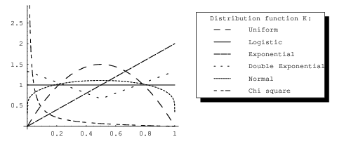
From Figure 3 we can deduce which $\phi$ -coefficients are given most weight for different marginal distributions. As the reference marginal, we take the logistic, which is the horizontal line in the figure, i.e., assigning uniform weights. We see that for a uniform marginal, the weight goes to zero in the tails. The weights for a normal marginal are for most $u$ intermediate between the weights for the uniform and logistic marginals. In contrast to uniform and normal marginals, the Laplace distribution gives more weight to the tails than a logistic marginal. An exponential marginal gives little weight to the lower tail, but much weight to the upper tail. Finally, the chi-square distribution gives very large weight to the lower tail and very small weight to the upper tail. Among the distributions considered, the biggest difference is between the chi-square and the exponential distribution.

6 Data analysis: investigating the nature of the association

Gaining an understanding of the nature of an association between two random variables is probably best viewed as an art rather than a science, and in this section we present some visual tools based on $\rho^{*}$ and its components which may be helpful in reaching this objective. For an iid bivariate sample $\{(X_{i},Y_{i})\}$ we propose the following two procedures.

Firstly, we calculate $\hat{\rho}^{*}$ from the sample and test its significance. If found to be significant, then for each data point $(X_{i},Y_{i})$ we calculate the weight

\displaystyle W_{i}=\frac{\frac{1}{n}\sum_{j=1}^{n}h_{\hat{F}_{1}}(X_{i},X_{j})\,h_{\hat{F}_{2}}(Y_{i},Y_{j})}{\sqrt{\hat{\kappa}(X,X)\,\hat{\kappa}(Y,Y)}}

Since

\displaystyle\hat{\rho}^{*}(X,Y)=\frac{1}{n}\sum_{i=1}^{n}W_{i}

the weights $W_{i}$ give an indication of how much the sample element $(X_{i},Y_{i})$ contributes to $\hat{\rho}^{*}$ , and so can be used to discover the nature of a possible association between $X$ and $Y$ .

Secondly, we calculate the component correlations $\hat{\rho}_{kl}$ of $\hat{\rho}^{*}$ and test their significance using the Bonferroni corrections described in Section 4.4. Then for each significant component correlation $\hat{\rho}_{kl}$ , we compute the weights

\displaystyle W_{i}^{(k,l)}=\hat{g}_{1k}(X_{i})\hat{g}_{2l}(Y_{i})

where $g_{1k}$ and $g_{2l}$ are the eigenfunctions belonging to $h_{F_{1}}$ and $h_{F_{2}}$ . Since

\displaystyle\hat{\rho}_{kl}=\frac{1}{n}\sum_{i=1}^{n}W_{i}^{(k,l)}

the weight $W_{i}^{(k,l)}$ is the amount the sample element $(X_{i},Y_{i})$ contributes to $\hat{\rho}_{kl}$ (conditionally on the marginals), and so, like $W_{i}$ , can be used to investigate the association between $X$ and $Y$ .

In this section we show how to visualize the weights $W_{i}$ and $W_{i}^{(k,l)}$ , both for continuous and categorical data, and show how this can be used to gain an understanding of the association. Some artificial continuous data sets are considered in Section 6.1, a real categorical data set is considered in Section 6.2 and a real time series data set is considered in Section 6.3

6.1 Some artificial data sets

In Figure 4, four artificial data sets are plotted, each consisting of 100 iid points. For completeness, we explain how the data were generated. In the following, $U$ is uniformly distributed on $[0,1]$ and $Z_{1}$ and $Z_{2}$ are iid standard normal random variables, and $Z(u)$ has a normal distribution with mean zero and standard deviation $u$ . The data in Figure 4(a) are from a bivariate normal distribution with $\rho=2/3$ . The data in Figure 4(b) are of the form $(X,Y)=(U,(U-1/2)^{2})+(Z_{1}/10,Z_{2}/10)$ . The data in Figure 4(c) are of the form $(X,Y)=(U,Z(1/5+U))$ . Finally, the data in Figure 4(d) are of the form $(X,Y)=(U,Z(1/5+\min\{U,1-U\}))$ .

For all four data sets, we performed permutation tests for the significance of $\hat{\rho}^{*}$ and its component correlations $\hat{\rho}_{ij}$ based on 10,000 random permutations. This took us about 48 minutes for each data set. For the significant component correlations we took 1 million random permutations to get a more accurate $p$ -value, and this took about 110 seconds per component correlation. We also computed the ordinary correlation, and, not surprisingly, only for the data in Figure 4(a) it is significantly different from zero. There we found that $\hat{\rho}=.44$ ( $p=.000$ ).

For the data in Figure 4(a), we found that $\hat{\rho}^{*}=.36$ ( $p=.000$ ), i.e., there is significant association. In Figure 5(a), the data are plotted again, this time each sample element $(X_{i},Y_{i})$ is represented with size proportional to $|W_{i}|$ ; black dots represent positive $W_{i}$ and white represent negative $W_{i}$ . In all these plots, the total area of the dots is scaled to a constant to make it easier to study them. From Figure 5(a),we see that the association seems to consist of a linearity in the data. It may be worthwhile however to check if there are other forms of association present by looking at the component correlations of $\hat{\rho}^{*}$ . We found two significant components: $\hat{\rho}_{11}=.61$ ( $p=.000$ ) and $\hat{\rho}_{22}=.38$ ( $p=.004$ ). In Figures 6(a) and 6(b) the weights $W_{i}^{(11)}$ and $W_{i}^{(22)}$ are visualized. The interpetation of the black and white dots is the same as above. The gridlines correspond to the zeroes of the marginal eigenfunctions. Therefore, within any rectangle the dots have the same color. Also in this case, the plots point to a linearity in the data.

For the data in Figure 4(b), we found $\hat{\rho}^{*}=.17$ ( $p=.000$ ) and we found two significant component correlations: $\hat{\rho}_{21}=-.78$ ( $p=.000$ ) and $\hat{\rho}_{42}=.54$ ( $p=.000$ ). The plots in Figures 5(b), 6(c) and 6(d) all point to a curved relationship.

For the data in Figure 4(c), we found that $\hat{\rho}^{*}=.11$ ( $p=.001$ ). There is significant association at the 5% level, but the evidence is not as overwhelming as in the previous two cases. We only found one significant component correlation: $\hat{\rho}_{12}=-.51$ ( $p=.000$ ). Figures 5(c) and 6(e) both point towards and increase in dispersion of the $Y$ variable as $X$ increases.

For the data in Figure 4(d), we found that $\hat{\rho}^{*}=.02$ ( $p=.522$ ). This time, the test based on $\rho^{*}$ does not yield a significant association. However, there is one significant component correlation: $\hat{\rho}_{22}=-.38$ ( $p=.004$ ). Figure 6(f) indicates that the association is due to an increase and then decrease in dispersion. Since $\hat{\rho}^{*}$ is not significant, we should refrain from giving an interpretation based on Figure 5(d).

For comparative purposes, we plotted the weights $W_{i}$ for data drawn from a distribution satisfying independence in Figure 7. Both sets consist of 100 sample elements. The most common pattern is that of Figure 7(a), with two diagonally opposing clusters of black dots and two diagonally opposing clusters of white dots. In a very limited investigation, this type of pattern occured about half of the time. Otherwise more complex patterns were obtained, such as the one in Figure 7(b). These figures indicate that it doesn’t seem to make sense to interpret this kind of plot if $\hat{\rho}^{*}$ is not significant, such as Figure 5(d).

Concluding, we see that significance tests combined with an inspection of the two types of plots in Figures 5 and 6 can give us insight into the kind of association present between two random variables.

6.2 Mental health data

	Mental Health Status
Parents’		Mild	Moderate
Socioeconomic		Symptom	Symptom
Status	Well	Formation	Formation	Impaired
A (high)	64	94	58	46
B	57	94	64	40
C	57	105	65	60
D	72	141	77	94
F	36	97	54	78
G (low)	21	71	54	71

Table 3: Cross-classification of Mental Health Status and Socioeconomic Status

Table 3 describes the relationship between child’s mental impairment and parents’ socioeconomic status for a sample of residents of Manhattan (\BCAYGoodmanGoodman1985; \BCAYAgrestiAgresti2002, and references therein). Goodman used this table to illustrate various association models for categorical data, including the so-called linear by linear association model, the row and columns effects model, and correspondence analysis based on canonical correlations. Here we illustrate the use of $\hat{\rho}^{*}$ and its components as yet an alternative method for analyzing these data. We relied on asymptotic $p$ -values because with 1670 observations approximate evaluation of the permutation tests would have been too time consuming using our implementation.

In the categorical case, for an $I\times J$ contingency table, it suffices to calculate weights for the cells, i.e., it is not necessary to calculate separately a weight for each individual observation. For an observation $(X_{i},Y_{i})$ in cell $(a,b)$ , the weight $W_{i}$ reduces to

\displaystyle W_{ab}=p_{ab}\frac{\sum_{i=1}^{I}\sum_{j=1}^{J}p_{ij}h_{\hat{F}_{1}}(i,a)h_{\hat{F}_{2}}(j,b)}{\sqrt{\hat{\kappa}(X,X)\hat{\kappa}(Y,Y)}}

where $p_{ab}$ is the proportion of observations in cell $(a,b)$ . Similarly, the weights belonging to component correlation $\rho_{kl}$ are

\displaystyle W_{ab}^{(k,l)}=p_{ab}g_{1k}(a)g_{2l}(b)

for $a=1,\ldots,I$ , $b=1,\ldots,J$ , $k=1,\ldots,I$ and $l=1,\ldots,J$ . Note that

\displaystyle\rho^{*}=\sum_{a=1}^{I}\sum_{b=1}^{J}W_{ab}

and

\displaystyle\rho_{kl}=\sum_{a=1}^{I}\sum_{b=1}^{J}W_{ab}^{(k,l)}

We found that $\hat{\rho}^{*}=.02$ ( $p=.000$ ), i.e., there is significant association in the data. The weights $W_{ab}$ for the cells are represented in Figure 8(a). Here, the grayscale represents the size of $W_{ab}$ : the darker the cell, the larger $W_{ab}$ ; $W_{ab}=0$ is represented by a fixed intermediate shade of gray. From Figure 8(a), it can be seen that most of the association is of a monotone nature: the higher the parents’ socioeconomic status, the better the mental health status of their children. We also investigated the component correlations and found two components to be significant at the 5% level: $\hat{\rho}_{11}=.13$ ( $p=.000$ ) and $\hat{\rho}_{13}=.08$ ( $p=.026$ ). In Figures 8(b) and 8(c) we represented the $W_{ab}^{(11)}$ and $W_{ab}^{(13)}$ using grayscales as above. From Figure 8(b), we see that $\hat{\rho}_{11}$ indicates linearity again. However, in Figure 8(c) we see evidence of some nonlinearity in the data, namely an apparent reversal of the association if only the middle categories ‘Mild Symptom Formation’ and ‘Moderate Symptom Formation’ are considered. Hence, it appears that the association which is present in the data cannot be fully explained by linearity.

6.3 Norwegian stock exchange

The Norwegian stock exchange data represented in Figure 9(a) yield an example with an especially interesting form of association. In Figure 9(a) the original time series data $Y_{t}$ are plotted. In Figure 9(b) we plotted

\displaystyle(Z_{t},W_{t})=(\mbox{arcsinh}(Y_{t}-Y_{t-1}),\mbox{arcsinh}(Y_{t+1}-Y_{t}))

The arcsinh transformation was done to make the marginal distributions less heavy tailed. We found a highly significant association with $\hat{\rho}^{*}(Z,W)=.09$ ( $p=.000$ ). From Figure 9(b) we can already interpret the association: large jumps (up or down) in stock prices tend to be followed by large jumps, and small jumps by small jumps, indicating periods of volatility. In Figure 9(c), the weights $W_{i}$ are represented by the size and color of the dots (see Section 6.1 for further explanation). This plot points to the same conclusion that large jumps are followed by large jumps and small jumps by small jumps. Note that in this case, not only the positive weights (the black dots) but also the negative weights (the white dots) are highly indicative of association. The plot indicates that the up-arm (with the black dots) is ‘heavier’ than the down-arm (with the white dots), that is, there is evidence that in the data generating process a jump tends to be of the same sign as the previous jump.

Seven component correlations were found to be significant at the 5% level after applying the Bonferroni correction: $\hat{\rho}_{11}=.25$ , $\hat{\rho}_{12}=.13$ , $\hat{\rho}_{22}=.64$ , $\hat{\rho}_{24}=.19$ , $\hat{\rho}_{33}=.19$ , $\hat{\rho}_{44}=.38$ and $\hat{\rho}_{66}=.25$ , all with $p=.000$ . In Figure 10, the weights corresponding to the component correlations are represented. Figures 10(c), (d), (f) and (g) point to the cross-like nature of the data. Figures 10(a) and (e) indicate that the up-arm is heavier than the down-arm. We did not find a meaningful explanation for Figure 10(b).

6.4 Discussion

If a researcher investigating the association between two variables decides on the use of $\rho^{*}$ , we recommend the following approach. First a test of the significance of $\hat{\rho}^{*}$ should be done, and, if found to be significant, the weights $W_{i}$ should be visualized as described above in order to determine the nature of the association. If this does not yield the desired insight, it can be worthwhile to investigate the component correlations and visualize the corresponding weights $W_{i}^{(k,l)}$ . These components form a (unique) orthogonal decomposition of the ‘infinite-dimensional’ object $\rho^{*}$ into ‘one-dimensional’ objects $\rho_{kl}$ , and the orthogonality ensures, in a limited sense, that the different components measure different things; by the latter we mean that for large samples and close to independence, the sample component correlations are approximately independent. The question may arise: why not investigate correlations between other sets of orthogonal functions? A sketch of an answer is as follows. Because of the various optimality properties of the eigenfunctions in describing the marginal kernels, these component correlations are likely to be a better choice for investigating the deviation of $\rho^{*}$ from zero than correlations between arbitrarily chosen functions for the marginal distributions. One way to make this intuitive is as follows: in those regions where the marginal distributions are sparse, the eigenfunctions vary relatively slowly (in second derivative sense, see remark after Lemma 7), and therefore power of a test based on a component correlation will be concentrated in those regions where there are many observations. Thus, if we believe $\rho^{*}$ to be a good measure of deviation from independence, then good ‘one-dimensional’ objects to look at are the correlations between the marginal eigenfunctions of $h_{F_{1}}$ and $h_{F_{2}}$ .

Acknowledgements

The author would like to thank the following institutes where he has been employed for providing a stimulating environment in which to carry out this research: The Methodology Department of the Faculty of Social Sciences at Tilburg University (Tilburg, the Netherlands) and EURANDOM (Eindhoven, the Netherlands).

References

(1) Agarwal, R. P. (1992). \BemDifference equations and inequalities. New York: Marcel Dekker.
(2) Agresti, A. (1992). A survey of exact inference for contingency tables. \BemStatistical Science, \BemVol. 7, No. 1, 131-177.
(3) Agresti, A. (2002). \BemCategorical Data Analysis, 2nd edition. New York: Wiley.
(4) Anderson, T. W. & Darling, D. A. (1952). Asymptotic theory for certain ‘goodness of fit’ criteria based on stochastic processes. \BemAnn. Math. Stat., \Bem47, 193-212.
(5) Baglivo, J., Pagano, M. & Spino, C. (1996). Permutation distributions via generating functions, with applications to sensitivity analysis of discrete data. \BemJ. Am. Stat. Ass., \Bem91, 1037-1046.
(6) Baringhaus, L. & Franz, C. (2004). On a new multivariate two-sample test. \BemJournal of multivariate analysis, \Bem88, 190-206.
(7) Blum, J. R., Kiefer, J. & Rosenblatt, M. (1961). Distribution free tests of independence based on the sample distribution function. \BemThe annals of mathematical statistics, \Bem32, 485-498.
(8) Booth, J. G. & Butler, R. (1999). An importance sampling algorithm for exact conditional tests in log-linear models. \BemBiometrica, \Bem86, 321-332.
(9) Bose, R. C. & Gupta, S. S. (1959). Moments of order statistics from a normal population. \BemBiometrika, \Bem46, 433 - 440.
(10) De Wet, T. (1980). Cramér-von Mises tests for independence. \BemJ. Multivariate Anal., \Bem10, 38-50.
(11) De Wet, T. (1987). Degenerate U- and V-statistics. \BemSouth African Statistical Journal, \Bem21, 99-129.
(12) De Wet, T. & Venter, J. H. (1973). Asymptotic distributions for quadratic forms with application to tests of fit. \BemAnnals of Statistics, \Bem1, 380-387.
(13) Deheuvels, P. (1981). An asymptotic decomposition for multivariate distribution-free tests of independence. \BemJ. Multivariate Anal., \Bem11, 102-113.
(14) Diaconis, P. & Sturmfels, B. (1998). Algebraic algorithms for sampling from conditional distributions. \BemAnn. Stat., \Bem13, 363-397.
(15) Durbin, J. & Knott, M. (1972). Components of the Cramér-von Mises statistics, I. \BemJ. R. Statist. Soc. B, \Bem34, 260-307.
(16) Eagleson, G. K. (1979). Orthogonal expansions and U-statistics. \BemAustralian Journal of Statistics, \Bem21, 221-237.
(17) Forster, J. J., McDonald, J. W. & Smith, P. W. F. (1996). Monte Carlo exact conditional tests for log-linear and logistic models. \BemJ. Roy. Stat. Soc. Ser B, \Bem58, 445-453.
(18) Goodman, L. A. (1985). The analysis of cross-classified data having ordered and/or unordered categories: association models, correlation models, and asymmetry models for contingency tables with or without missing entries. \BemAnn. Stat., \Bem13, 10-69.
(19) Govindarajulu, Z. (1963). On moments of order statistics and quasi-ranges from normal populations. \BemAnn. Math. Statist., \Bem34, 633-651.
(20) Gregory, G. G. (1977). Large sample theory for U-statistics. \BemAnnals of Statistics, \Bem5, 110-123.
(21) Hall, P. (1979). On the invariance principle for U-statistics. \BemStoch. Proc. Appl., \Bem9, 163-174.
(22) Hoeffding, W. (1940). Masstabinvariante Korrelationtheorie. \BemSchriften Math. Inst Univ. Berlin, \Bem5, 181-233.
(23) Hoeffding, W. (19481). A class of statistics with asymptotically normal distribution. \BemAnnals of Mathematical Statistics, \Bem19, 293-325.
(24) Hoeffding, W. (19482). A non-parametric test of independence. \BemAnnals of Mathematical Statistics, \Bem19, 546-557.
(25) Hoeffding, W. (1961). The strong law of large numbers for U-statistics. \BemInstitute of Statistics, University of North Carolina, Mimeograph Series No. 302.
(26) Johnson, Kotz & Balakrishnan. (1994). \BemContinuous univariate distributions: volume 1. New York: Wiley.
(27) Kallenberg, W. C. M. & Ledwina, T. (1999). Data driven rank tests for independence. \BemJ. Amer. Statist. Assoc., \Bem94, 285-301.
(28) Kiefer, J. (1959). $K$ -sample analogues of the Kolmogorov-Smirnov and Cramér-von Mises tests. \BemAnn. Math. Stat., \Bem30, 420-447.
(29) Mikosch, T. (2006). Copulas: tales and facts (with discussion). \BemExtremes, \BemTo appear.
(30) Nelsen, R. B. (2006). \BemAn introduction to copulas. New York: Springer.
(31) Neyman, J. (1937). “Smooth” tests for goodness of fit. \BemSkand. Aktuarietidskr., \Bem20, 150-199.
(32) Randles, R. H. & Wolfe, D. A. (1979). \BemIntroduction to the theory of nonparametric statistics. New York: Wiley.
(33) Rüschendorf, L. (1991). Fréchet bounds and their applications. In G. Dall’Aglio, S. Kotz & G. Salinetti (Eds.), \BemAdvances in probabability distributions with given marginals (p. 151-188). Kluwer.
(34) Tricomi, F. G. (1985). \BemIntegral equations. Dover Publications.
(35) Van de Wiel, M. A., Di Bucchianico, A. D. & Van der Laan, P. (1999). Symbolic computation and exact distributions of nonparametric test statistics. \BemThe statistician, \Bem48, 507-516.
(36) Weisstein, E. W. (1999). “Erf” and “Erfi”. \BemFrom MathWorld–A Wolfram Web Resource. http://mathworld.wolfram.com/Erfi.html.
(37) Zaanen, A. (1960). \BemLinear analysis. Amsterdam: North Holland Publishing Co.
(38) Zech, G. & Aslan, B. (2003). A multivariate two-sample test based on the concept of minimum energy. \BemPHYSTAT2003, 97-100.

1 Introduction

2 Properties of the kernel function hFh_{F}

2.1 Key properties of hFh_{F}

Lemma 1

Lemma 2

Lemma 3

Lemma 4

2.2 Spectral decomposition of hFh_{F}

Theorem 1

Lemma 5

Example 1

Lemma 6

Corollary 1

2.3 Obtaining the eigensystem in the discrete case

Lemma 7

2.4 Obtaining the eigensystem in the continuous case

Lemma 8

Lemma 9

Example 2

2.5 Discrete approximation of the continuous case

2.6 Relation to Anderson-Darling kernel

3 Properties of κ\kappa and ρ∗\rho^{*}

3.1 Key properties of κ\kappa and ρ∗\rho^{*}

Theorem 2

Corollary 2

Lemma 10

3.2 Orthogonal decomposition

Theorem 3

3.3 Parameterization of the likelihood

3.4 Fréchet bounds for component correlations

Lemma 11

Example 3

Example 4

4 Estimation and tests of independence

4.1 U and V statistic estimators of κ\kappa

4.2 Permutation tests

4.3 Asymptotic distribution of estimators under independence

Theorem 4

4.4 Bonferroni corrections for testing significance of component correlations

5 Grade versions of κ\kappa and ρ∗\rho^{*}, copulas, and rank tests

5.1 Rank tests

5.2 A new class of KK-sample Cramér-von Mises tests as a special case

5.3 κ\kappa as a weighted ϕ\phi-coefficient

6 Data analysis: investigating the nature of the association

6.1 Some artificial data sets

6.2 Mental health data

6.3 Norwegian stock exchange

6.4 Discussion

Acknowledgements

References

2 Properties of the kernel function $h_{F}$

2.1 Key properties of $h_{F}$

2.2 Spectral decomposition of $h_{F}$

3 Properties of $\kappa$ and $\rho^{*}$

3.1 Key properties of $\kappa$ and $\rho^{*}$

4.1 U and V statistic estimators of $\kappa$

5 Grade versions of $\kappa$ and $\rho^{*}$ , copulas, and rank tests

5.2 A new class of $K$ -sample Cramér-von Mises tests as a special case

5.3 $\kappa$ as a weighted $\phi$ -coefficient