On the reduction of a random basis

To the independent system $b_{1}^{(n)},b_{2}^{(n)},\dots,b_{p}^{(n)}$, the classical Gram-Schmidt orthogonalization procedure associates the orthogonal system $\widehat{b}_{1}^{(n)},\cdots,\widehat{b}_{p}^{(n)}$ defined by the recursion

If $B=[b_{1}^{(n)},\cdots,b_{p}^{(n)}]$ is the $n\times p$ matrix with column vectors $b_{1}^{(n)},\cdots,b_{p}^{(n)}$ in the canonical basis, this orthogonalization corresponds to the $QR$ decomposition $B=QR$ where

is an orthogonal $n\times p$ matrix and $R$ is an upper triangular $p\times p$ matrix $(R_{k,j}=0\ ,\ 1\leq j<k\leq n)$ and

Notice that these three models are cited in the book of Knuth ([9, Section 3.4.1]).

The lattice basis reduction problem deals with finding a basis of a given lattice, whose vectors are “short” and “almost orthogonal”. The problem is old and there are numerous notions of reduction. For a general survey, see for example [8, 16, 7]. Solving even approximately the lattice basis reduction problem has numerous theoretical and practical applications in integer optimization [11], computational number theory [10] and cryptography [14].

In 1982, Lenstra, Lenstra and Lovász [10] introduced for the first time an efficient (polynomial with respect to the length of the input) approximation reduction algorithm. It depends on a real approximation parameter $s\in]0,\sqrt{3}/{2}[$ and is called LLL($s$). The output basis of the LLL algorithm is called an LLL($s$) reduced or $s$-reduced basis. In this paper we are concerned with the probability that a random basis under a spherical model is LLL$(s)$ reduced, (i.e. is already an output basis of the LLL($s$)-algorithm).
Roughly speaking the LLL reduction procedure is an approximation algorithm following a divide and conquer paradigm: Indeed for $i\in\{1\dots p-1\}$, the following condition (1.6) ensures that some “local two dimensional basis” is $s$-reduced. This two dimensional basis is the projections of $b_{i}^{(n)}$ and $b_{i+1}^{(n)}$ into the orthogonal $H_{i}^{\perp}$ of the vector space $H_{i}$ spanned by $b_{1}^{(n)},b_{2}^{(n)},\dots,b_{i-1}^{(n)}$. [10] showed that when all these two–dimensional bases are $s$-reduced then the whole basis has nice enough Euclidean properties. For instance, the length of the first vector of an LLL-reduced basis is not longer than $(1/s)^{(p-1)}$ times the length of a shortest vector in the lattice generated by $b_{1}^{(n)},b_{2}^{(n)},\dots,b_{p}^{(n)}$.

The next definition characterizes an LLL($s$) reduced basis.

Firstly in the original definition the basis has also to be proper, i.e. if $B=QR$ is the decomposition (1.2) associated with the Gram–Schmidt orthogonalization of the basis $b_{1}^{(n)},b_{2}^{(n)},\dots,b_{p}^{(n)}$, then

But from any basis satisfying (1.6) one efficiently obtains a proper basis still satisfying (1.6) by a straightforward sequence of integer translations provided in appendix. Moreover considering the notion of flag [7] rather than basis for lattices, makes it possible to skip the notion of properness.

Secondly the approximation parameter of the original LLL in [10] is slightly different from the one we use here and the reduction we consider here is indeed Siegel reduction as called in [2, 1]. Our main Theorem 1.4 is still true with the original definition of a LLL reduced basis as detailed in appendix.

In this paper we study the asymptotics (with respect to the dimension $n$ of the ambient space) of the random variables ${\cal M}_{n}^{g}$ and ${\cal I}_{n}^{g}$ under spherical models and for general codimensions of the random basis. The variable ${\cal M}_{n}^{g}$ is the supremum of the set of those $s$ for which the basis is $s^{2}$-reduced. As mentioned earlier an LLL($s$) reduced basis satisfies a set of local conditions. The second variable ${\cal I}_{n}^{g}$ is the place where the satisfied local condition is the weakest. This indicates where the limitation of the reduction comes from locally.

Notice that in [6], Donaldson proved a phenomenon similar to the assertion $(i)$ of Theorem 1.4. He considered a different random model: The basis $b_{1}^{(n)},\cdots,b_{n-g}^{(n)}$ is picked up uniformly in the set $\{\|b_{1}^{(n)}\|^{2}+\cdots+\|b_{n-g}^{(n)}\|^{2}=1\}$ (Euclidean sphere in $\mathbb{R}^{n\times(n-g)}$). He proved that as $n\rightarrow\infty$ with $n-g(n)$ a fixed constant , the basis is asymptotically reduced in the sense of Minkowski, i.e. each $b_{i}^{(n)}$ is a shortest vector among all vectors of the lattice that complete $b_{1}^{(n)},\cdots,b_{i-1}^{(n)}$ to form a bigger subset of a lattice basis. So his result is about a stronger notion of reduction but he considered a much more restricted class of basis.

To finish this Section about lattice basis reduction, observe that our Theorem 1.4 about LLL reduction can be generalized to other reductions: In [15] Schnorr introduces a new type of reduction by segments. In this setting one fixes an integer $k$ and partitions a basis whose vectors are in $\mathbb{R}^{n}$ and whose codimension is $g$ into $m$ segments of $k$ consecutive basis vectors such that $n-g=km$. For a basis with codimension $g$, the reduction criterion is based on the quantity

Similarly to the assertions of Theorem 1.4, if $g=g(n)$ tends to infinity and the block size $k$ is fixed, then for any $s\in[0,1]$ the probability that a random basis is $s$–reduced in the sense introduced by Schnorr tends to $1$ with $n$. If $g$ is constant then this probability tends to a constant in $[0,1]$ (depending on $s$, $g$ and $k$). ¹¹ 1 Of course there is a choice of approximation parameters such that when a basis is LLL($s$) reduced then for any fixed $k$, it is also $s,k$-reduced in the sense introduced by Schnorr. But our approach here shows the existence of limit probabilities (with $n$) for the reduceness of a random basis in the sense introduced by Schnorr.

The random variable ${\cal M}_{n}^{g}$ has the representation :

As one can guess in view of Theorem 1.5, under $\nu_{n}$, for each $j$, $r_{j}^{(n)}$ converges in distribution to $\gamma\left(\frac{j+1}{2}\right)/{\gamma\left(\frac{j}{2}\right)}\,,$ where $\gamma\left(\frac{j+1}{2}\right)$ and $\gamma\left(\frac{j}{2}\right)$ are independent (see Proposition 2.1). By the strong law of large numbers, one sees that $\gamma\left(\frac{j+1}{2}\right)/{\gamma\left(\frac{j}{2}\right)}\xrightarrow[j]{a.s.}1$; this allows to guess that the minimum ${\cal M}_{n}^{g}$ is reached by the firsts $r_{j}^{(n)}$; this motivates the time inversions done in (1.12).

The variable ${\cal M}_{n}^{g}$ is a function of the $(n-g)$-tuple $(r_{g+1}^{(n)},\cdots r_{n-1}^{(n)})$, and then the convergence of each coordinate is not sufficient to yield that of ${\cal M}_{n}^{g}$. We have to take into account that the variables $(r_{j}^{(n)})_{j\leq n-1}$ are dependent, and that their number is growing. Since for the ”last” indices ($n-i$ with $i$ fixed), $r_{n-i}^{(n)}\xrightarrow[n]{~(d)~}1$ (see (2.4)), it is convenient to embed the $(n-1)$-tuple $(r_{1}^{(n)},\cdots r_{n-1}^{(n)})$ into $\mathbb{R}_{+}^{{I\!N}}$ (the set of infinite sequences of positive real numbers), setting

Let $(\eta_{i})_{i\geq 1}$ be a sequence of independent random variables such that $\eta_{i}\mathrel{\mathop{\kern 0.0pt=}\limits^{(d)}}\gamma_{i/2}$ and set

We denote by $\|.\|_{p}$ the classical norm on the set $\ell_{p}$ of sequences of real numbers with finite $p$th moment: for any sequence of real numbers ${\sf x}=({\sf x}_{i})_{i\geq 1}$, $\|{\sf x}\|_{p}$ is $\left(\sum_{i\geq 1}|{\sf x}_{i}|^{p}\right)^{1/p}$ and $\ell_{p}$ is $\{{\sf x},\|{\sf x}\|_{p}<+\infty\}$.

For $k\in{I\!N}$, set

The application ${\sf x}\mapsto 1+\min_{i\geq k}{\sf x}_{i}$ is continuous from $\ell_{p}$ onto $\mathbb{R}$. It follows that ${\cal M}_{n}^{g}\wedge 1$ converges in distribution to ${\cal M}^{g}$. We will prove that

Notice that Proposition 1.7 and Theorem 1.8 have their analogous for the reduction introduced by Schnorr in [15]. By setting

if we let $n\rightarrow\infty$, we have convergence of $(r_{k,r}^{(n)})_{r}$ to a process $({\cal R}_{k,r})_{r}$ with

where the $\eta_{k,r},r\geq 1$ are independent, and the gamma variables too. Then by setting

one obtains also an analogous to Theorem 1.8.

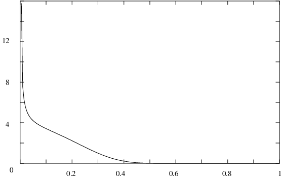
A note on the proof of Proposition 1.7. The ambient spaces $\mathbb{R}^{n},n\geq 1$ are not nested, and then we give up the geometrical consideration on $\mathbb{R}^{n}$ and focus on the representation of the processes $r_{j}^{n}$ using the gamma distributions.

Proof of Theorem 1.5: Let us skip the superscript $(n)$ in this proof. We have $b_{i}=\theta_{i}\|b_{i}\|$ and from (1.1), we see that $\widehat{b}_{i}=\|b_{i}\|\widehat{\theta}_{i}$, where the $\widehat{\theta}_{i}$’s are obtained by the Gram-Schmidt algorithm applied to the $\theta_{i}$’s. The independence of $(\widehat{\theta}_{1},\cdots,\widehat{\theta}_{n})$ and $(\|b_{1}\|^{2},\cdots,\|b_{n}\|^{2})$ is then a direct consequence of the radial-angular independence. Notice that $\widehat{\theta}_{1}=1$.

Proof of Propositions 2.1 and 2.2 From Theorem 1.5 we have the decomposition,

with $Y_{n-j}^{(n)}\mathrel{\mathop{\kern 0.0pt=}\limits^{(d)}}\beta\left(\frac{j+1}{2},\frac{n-j-1}{2}\right)\,.$ Let $(\xi_{j})_{j\geq 1}$ be a sequence of i.i.d. $\gamma_{1/2}$-distributed random variables. From (3.3) and (3.2), we can write

By the strong law of large numbers,

and for each $j$, $\sum_{m=1}^{j+1}\xi_{m}\mathrel{\mathop{\kern 0.0pt=}\limits^{(d)}}\gamma((j+1)/2)$, which yields (2.1). From this and the additional assumption $\|b_{1}^{(n)}\|^{2}/a_{n}\xrightarrow[n]{~(d)~}1$, we see that (2.3) holds true. For (2.2), notice that $(1-Y_{j}^{(n)})\mathrel{\mathop{\kern 0.0pt=}\limits^{(d)}}Y_{n-j+2}^{(n)}\,,$ and that $Y_{n-j+2}^{(n)}\xrightarrow[n]{proba.}0$ by (2.1). To end, (2.4) is a consequence of (2.2) and $\|b_{1}^{(n)}\|^{2}/a_{n}\mathrel{\mathop{\kern 0.0pt\to}\limits^{(d)}}1$. $\Box$

Proof: We have

as soon as $\rho\leq 1/2$. Similarly

With the help of assumption (1.4), this yields

$\Box$

References

- [1] A. Akhavi. Analyse comparative d’algorithmes de réduction sur les réseaux aléatoires. PhD thesis, Université de Caen, 1999.
- [2] A. Akhavi. Random lattices, threshold phenomena and efficient reduction algorithms. Theoretical Computer Science, 287:359–385, 2002.
- [3] N.R. Chaganthy. Large deviations for joint distributions and statistical applications. Sankhya, 59:147–166, 1997.
- [4] L. Chaumont and M. Yor. Exercises in probability. Cambridge Series in Statistical and Probabilistic Mathematics. Cambridge University Press, Cambridge, 2003. A guided tour from measure theory to random processes, via conditioning.
- [5] H. Daudé and B. Vallée. An upper bound on the average number of iterations of the LLL algorithm. Theor. Comput. Sci., 123(1):95–115, 1994.
- [6] J.L. Donaldson. Minkowski reduction of integral matrices. Mathematics of Computation, 33(145):201–216, 1979.
- [7] Jr. H.W. Lenstra. Flags and lattice basis reduction. In European Congress of Mathematics, Vol. I (Barcelona, 2000), volume 201 of Progr. Math., pages 37–51. Birkhäuser, Basel, 2001.
- [8] R. Kannan. Algorithmic geometry of numbers. In Annual review of computer science, Vol. 2, pages 231–267. Annual Reviews, Palo Alto, CA, 1987.
- [9] D. E. Knuth. The art of computer programming. Vol. 2. Addison-Wesley Publishing Co., Reading, Mass., second edition, 1981. Seminumerical algorithms, Addison-Wesley Series in Computer Science and Information Processing.
- [10] A. K. Lenstra, H. W. Lenstra, Jr., and L. Lovász. Factoring polynomials with rational coefficients. Math. Ann., 261(4):515–534, 1982.
- [11] H. W. Lenstra, Jr. Integer programming and cryptography. Math. Intelligencer, 6(3):14–19, 1984.
- [12] G. Letac. Isotropy and sphericity: some characterisations of the normal distribution. Ann. Statist., 9(2):408–417, 1981.
- [13] R. J. Muirhead. Aspects of multivariate statistical theory. John Wiley, 1982.
- [14] P. Q. Nguyen and J. Stern. The two faces of lattices in cryptology. In Cryptography and lattices (Providence, RI, 2001), volume 2146 of Lecture Notes in Comput. Sci., pages 146–180. Springer, 2001.
- [15] C.P. Schnorr. Fast LLL-Type Lattice Reduction. Information and Computation, 204:1–25, 2006.
- [16] B. Vallée. Un problème central en géometrie algorithmique des nombres: la réduction des réseaux. Autour de l’algorithme de Lenstra Lenstra Lovasz. In Informatique Théorique et Applications, volume 3, pages 345–376. 1989. English translation by E. Kranakis CWI-Quaterly - 1990 - 3.