On Pseudospectra of Matrix Polynomials
and their Boundaries
Lyonell Boulton
Affiliation: Department of Mathematics and the Maxwell Institute for Mathematical
Sciences,Affiliation: Heriot-Watt University, Edinburgh EH14 2AS, United Kingdom.Peter Lancaster
Affiliation: Department of Mathematics and Statistics,Affiliation: University of Calgary, Calgary AB, Canada T2N 1N4.Panayiotis Psarrakos
Affiliation: Department of Mathematics, National Technical University,Affiliation: Zografou Campus, 15780 Athens, Greece.
Abstract
In the first part of this paper (Sections 2-4), the
main concern is with the boundary of the pseudospectrum of a
matrix polynomial and, particularly, with smoothness properties of
the boundary. In the second part
(Sections 5-8), results are obtained
concerning the number of connected components of pseudospectra,
as well as results concerning matrix polynomials with multiple
eigenvalues, or the proximity to such polynomials.
Keywords:
Matrix polynomials, perturbation of eigenvalues, singular values,
pseudospectra.
This paper falls into two parts. In the first
(Sections 2-4), the main concern is with the
boundary of the pseudospectrum of a matrix polynomial and,
particularly, in view of its importance for boundary-tracing
algorithms, with the smoothness properties of the boundary. In
the second (Sections 5-8), we further
develop analysis begun by two of the present authors (see
[13]) on qualitative aspects of the pseudospectrum. This
part is also influenced by earlier work on pseudospectra for
standard eigenvalue problems by Alam and Bora in [3]. In
particular, results are presented concerning the number of
connected components of the pseudospectrum and proximity to
systems with multiple eigenvalues.
Let us begin with some formal definitions. First, a matrix
polynomial is a function (the
algebra of all complex matrices) of the form
(1)
where is a complex variable and with . The spectrum of such a function is .
Since consists of no more than
distinct eigenvalues. A nonzero vector
is known as an eigenvector of
corresponding to an eigenvalue if it
satisfies . The algebraic multiplicity
of a is the multiplicity of as a
zero of the scalar polynomial , and it is always
greater than or equal to the geometric multiplicity of
, that is, the dimension of the null space of the matrix
. A multiple eigenvalue of is called
defective if its algebraic multiplicity exceeds its
geometric multiplicity.
We let denote the linear space of matrix
polynomials with degree or less. Using the spectral matrix
norm (i.e., that norm subordinate to the Euclidean vector norm),
we may define the max norm on ,
(2)
Using this norm, we construct a class of matrix polynomials
obtained from in (1) by perturbation. The
admissible perturbations are defined in terms of a real polynomial
with nonnegative coefficients and a
positive constant coefficient; for each
and . First consider matrix
polynomials in of the form
(3)
where the matrices
() are arbitrary. Then, for a given the class of admissible perturbed matrix polynomials is
(4)
This is a convex compact set in the linear space with the
norm (2).
The -pseudospectrum ofwith respect to
(introduced by Tisseur and Higham [18]) is then
(5)
As is generally fixed throughout this paper, it
will not appear explicitly in this notation, and we will refer to
simply as the -pseudospectrum of . Note
that if then all matrix
polynomials in have nonsingular leading
coefficients, and this ensures that is bounded (Theorem 2.2
of [13]).
If we define the standard eigenvalue problem as that in
which then it is natural to define weights
(no perturbation of the coefficient is admitted)
and . Thus, and, using (5), we
obtain the relatively well-understood “-pseudospectrum of
matrix ”, namely,
2 The singular value functions
For any the singular values of a matrix
polynomial are the nonnegative square-roots of the
eigenvalue functions of . They are denoted by
The real-valued function
given by the smallest singular value, provides more information
about the matrix polynomial than alone.
This will become clear in the forthcoming section when we discuss
the pseudospectrum of . Let us first describe some
general properties of .
It is clear that an alternate definition of the spectrum of a
matrix polynomial is:
The connection between the zeros of and the eigenvalues
of can be made more precise using the singular value
decomposition.
Proposition 1
An eigenvalue has geometric multiplicity
if and only if
Our analysis depends on an important, concise characterisation of
the -pseudospectrum in terms of the function .
This was obtained by Tisseur and Higham (Lemma 2.1 of [18]),
(6)
Clearly, for any
. Thus, is nothing but the level set at height
of the real-valued function , or
that at height of the function . Notice also that in the standard eigenvalue
problem, in (6). More
generally, (in equation (6)) is a
radially symmetric non-decreasing function of .
By using the Euclidean vector norm,
(7)
Our first theorem has been originally established by Davies in the more general context of holomorphic families of
bounded operators. A proof is included here for completeness.
Theorem 2
Let be invertible on a domain . Then
is a subharmonic function on .
Proof. First we recall one of the characterisations
of continuous subharmonic functions (see Ahlfors [2], for
example). A continuous function is
subharmonic if and only if, for any closed disc in with centre
and radius ,
A well known result from operator theory establishes
that for any bounded linear operator on a Hilbert space,
If the Hilbert space is finite dimensional, it is easy to see that
the supremum is attained. By virtue of (7), . Thus,
(8)
Now note that is continuous on , and let
and be such that
The function is analytic on
and so the real function
(9)
is harmonic on . Furthermore, it follows from (8)
and (9) that on .
Consequently,
and the result follows.
An important characteristic of subharmonic functions is the fact
that they satisfy the maximum principle. Therefore, the only local
minima of are those .
The subharmonicity of has been considered
recently by various authors. In [5], Boyd and Desoer
discuss this property in the context of linear control systems.
Concrete applications of this theorem may be found
in [9] for the linear case, and in [4, 7] for the
quadratic case. In [4], the result is applied in support of a
certain novel procedure for finding eigenvalues of self-adjoint
operators in infinite dimensional Hilbert spaces.
Corollary 3
For all , every connected component of has
non-empty interior.
Proof. Suppose, on the contrary, that is a
connected component of with empty interior. Since
is subharmonic, should be attained at all points of .
Thus, necessarily, should be a single point and in fact one
of the eigenvalues of . The continuity of and
the fact that ensure that this is not possible.
In general, itself is not a subharmonic function as it
does not satisfy the maximum principle (a concrete example may be
found at the end of this section). However, as we will see next,
is locally regular.
First consider the nonnegative
eigenvalue functions generated on by the matrix function
, say . They
can be organised in such a way that they have a strong smoothness
property.
Lemma 4
For any given analytic curve the
eigenvalues of can be arranged in such way that,
for all , are real analytic functions of
.
Furthermore, if is a
non-zero simple singular value of and
are associated left and right singular
vectors, respectively, then (writing )
is a real analytic function in a neighbourhood of and
(10)
The first statement follows from Theorem S6.3 of [10] (see
also Theorem II-6.1 of [11]). For the second and third, see
[16], for example.
We can interpret the first part of this lemma pictorially in the
following manner. For the graphs of
() are smooth and might cross
each other. At a crossing point, the graph of the corresponding
singular value is continuous but it changes from
one smooth curve to another with a possible jump in the
derivative (see §II-6.4 of [11]).
We may also consider regularity properties of
as a function defined on the complex plane.
In this case, some rudimentary ideas from algebraic
geometry assist in
discussing the surfaces in which are (in general)
generated by the singular values. (Where possible, the terminology
of Kendig [12] is followed).
Write in real and imaginary parts; and define subsets of :
Proposition 5
The union is a real algebraic
variety.
Proof. Define the function
(11)
Since the matrix is hermitian,
is a polynomial in with real coefficients, and since
the result follows.
In spite of this proposition and Lemma 4, the
existence of an arrangement of the eigenvalues of such that the surfaces are
smooth everywhere is not guaranteed in general. Consider
the following example. For the linear matrix polynomial
where
has a conic double point at
. Therefore, no arrangement of the singular values
exists ensuring , and
are simultaneously smooth at . Moreover, in
this example, so note that the
hypothesis of non-degeneracy of the fundamental singular value in
the second part of Lemma 4 is essential.
For linear polynomials, the occurrence of isolated singularities
in is rare. In the above example the
matrix had to be carefully crafted to allow the conic double
point around the origin. Any slight change in the coefficients of
would eliminate this degeneracy.
The following useful proposition is an immediate consequence of
Lemma 4.
Proposition 6
If
for and for all in a non-empty open set
, then .
Thus, different surfaces can intersect only in sets of
topological dimension at most one.
3 The pseudospectrum and its boundary
Now we put these ideas into the context of the study of
pseudospectra.
A fundamentally important case is that in which is so
small that consists of “small” disconnected components,
each one containing a single (possibly multiple) eigenvalue of
. As is increased from zero, these components
enlarge, collide and eventually intersect in various ways so that
the boundary of , say , becomes more complex.
In an earlier paper [13] two of the present authors studied
some basic properties of and in support of a
curve-tracing algorithm for plotting .
Let
(12)
Since this function is continuous in it
follows from (6) that
(13)
Moreover, as long as is a simple
non-vanishing eigenvalue of , differentiation in
the direction of the boundary will be well-defined as a
consequence of Lemma 4. However, when this smoothness of the boundary may be lost.
Hence our interest in the set of for which
is multiple; curve tracing algorithms are prone to fail around
these points, as the directional derivatives along
may not be well-defined.
Even though it is quite rare111
This is a rather delicate
point, and it seems to have been missed in the work of several
preceding authors as in [13] and [18]. In particular,
Corollary 4.3 of [3] seems to be false as it stands. On the
other hand, this fact seems to have little, if any impact on the
design of algorithms., in general, the right side of
(13) might include points in the interior of .
This can be observed as a consequence of either of the two
unlikely events:
(i)
the surface having a local
(but not global) maximum,
(ii)
at least three multiple sheets of intersecting in a single point.
Demmel’s matrix
with illustrates (i) for the standard eigenvalue problem with
.
Indeed if and ,
has a local maximum at , cf. [8].
Higher order examples typifying (i) can also be easily constructed.
Consider, for instance, the polynomial
in and the weight function
. The point is a local maximum of
the function
which is smooth in . This may be verified by directly computing the
gradient and Hessian of this expression at . Thus, when
and lies in a sufficiently small neighbourhood
of the origin we have so that
and .
However, for ,
To confirm (ii), recall Example 3.5 of [3]: for
and any the -pseudospectrum of is the union of four
closed discs with centres at the eigenvalues
and radii equal to . Thus, for , the origin lies
in the set but it is an
interior point of .
The next result shows that is made up of
algebraic curves. This is a comforting property in the sense that
the number of difficult points, such as cusps or
self-intersections, is limited. (See Proposition 6.2.10 of
[6] for an explicit statement of this kind.)
Theorem 7
Let and assume that . Then the boundary of
lies on an algebraic curve. In particular,
is a piecewise curve, it has at most a finite number
of singularities where the tangent fails to exist, and it
intersects itself only at a finite number of points.
Proof.
We first show that lies on an algebraic curve.
Recall the function defined by
(11) and observe that lies on the level
set
The function can be written in the form
where and are real polynomials in .
Thus,
If is an even function, then is identically zero
and either is an algebraic curve or it coincides with the
complex plane. Suppose is not an even function. Then
is a subset of the level set
which is also an algebraic curve when it does not coincide with the
complex plane.
Next we show that only if . Thus, if
and , are not identically zero, then
where the order of the (irreducible) factor in the
left hand side is odd and the order of the same factor on the
right (if any) is even. This is a contradiction. Hence, if
then and are identically zero,
and consequently, .
Since and by hypothesis both and so is an
algebraic curve. This completes the first part of the theorem.
For the second part, note that, as is continuous in
, is a union of continuous
curves. From the above considerations it follows that is
a piecewise curve and it has finitely many
singularities. Then, since
we can actually decompose where () are suitable smooth
curves with the following property: for all and
for all
. Thus, as needed.
Note that for the standard eigenvalue problem, is
an even function. In this case, the above result appears in
the work of Alam and Bora [3].
The following technical statements will be useful subsequently.
The first one follows immediately from (13).
Lemma 8
If then and .
In particular, note that for any .
With as in (1), consider a perturbed matrix
polynomial of the form (3). It follows
from the definition (4) that if and only if
for each and equality holds for at least one .
Now consider matrix polynomials in the interior of ;
. It is easily seen that if and only if
Lemma 9
If then
for any perturbation such that
.
Proof. Let . It suffices to
show that if for a then for
some . Indeed, if we assume the converse
statement, for all , then
for some . But since we have which contradicts Lemma 8.
Thus, the desired assertion holds.
4 The fault lines
Differentiability along , the boundary of the
pseudospectrum, is possible as long as the gradient of
exists and does not vanish. The
only place where might fail to have a derivative is the
origin. If the minimal singular value, , has
multiplicity one, then is smooth in a neighbourhood of
. Thus, the study of those points where differentiability is
lost, apart from is confined to the region of the plane
where the sheet of corresponding to ,
meets the one corresponding to . This motivates the
following definition.
The rather involved indexing introduced next is required
to handle multiple eigenvalues.
Below we always assume that the eigenvalues of are ordered so that for all
. Let (usually not onto) satisfying the following
properties:
(a)
,
(b)
and
(c)
if and only if .
The map is a choice of the indices of those, and only those,
different . Let and
. We define the
set
By virtue of Proposition 6, has empty interior.
Furthermore, if all eigenvalues of have
geometric multiplicity equal to , then
Proposition 10
If all the eigenvalues of have geometric multiplicity
equal to , then either or lies
on an algebraic curve (including the possibility of isolated
points).
Proof. Let
so that . This set is the locus of all
points such that the discriminant of the real
polynomial in defined by (11) is zero.
The hypothesis ensures that and thus, either
or is an algebraic curve. The
result follows just because is a subset of .
In particular, might include straight lines,
single points, the empty set, or be a complicated set such as a
Voronoi diagram (see Example 1 below).
Borrowing a geological term, we call the set the set of
fault points of . In general, will be made up of
fault lines. The explicit determination of the fault lines
of requires computations with determinants and
discriminants, and is therefore unrealistic. However, the
following considerations demonstrate the role that the fault
lines frequently play in the study of pseudospectra.
Let be as in (12). As mentioned above, apart
from if does not exist, then . At these points, the curve will typically
fail to have a tangent line. There are other points where the
tangent line will be undefined, those where .
In this case, there is a saddle point in the minimal singular
value surface. These may or may not lie on
(see Section 6).
Example 3 below illustrates a case in which is a
singleton. In Example 4, is empty but there is,
nevertheless, a point at which has no tangent. In
Examples 1, 2, and 5, is, indeed, made up of
fault lines.
Example 1 Let be an normal
matrix with eigenvalues . Then the
fault lines of (i.e., for the standard
eigenvalue problem) form the Voronoi diagram defined by
(i.e., the boundary of their Dirichlet
tessellation).
Example 2 Naive experiments with diagonal
matrix polynomials provide an insight on the possible structure of
individual fault lines. For instance, let and set
.
Figure 1: The thin solid lines are . The thick
solid lines are .
In Figure 1, we depict the evolution of the set
and () for . The fixed eigenvalues
of are plotted as “+” and the perturbed eigenvalue
is marked with a “”.
In general, an unbounded appears to be more
likely to occur. Nonetheless this set can also contain a compact
smooth curve. In both of the lower figures,
consists of an unbounded curve, which is asymptotic to a vertical
line, and a closed compact curve on the right half plane around
the perturbed eigenvalue . The curve
has a self intersection at for . This can be shown from the fact that this part of the
pseudospectrum depends only on the first diagonal entry of
. The self intersection disappears as soon as moves
sufficiently close to . There are critical values of ,
where . Two of these critical values are
and .
Example 3 can also be a singleton.
In the left part of Figure 2, we depict
for the linear matrix polynomial
the weight function and . The very special structure of this matrix polynomial ensures
that . The boundary of the pseudospectrum
does not have a tangent line at when
. Compare with Example 4 below.
Figure 2: has no tangent line at the origin
for just one .
By construction, is independent of . Therefore, the
singularities occurring on in places where the
gradient of (12) fails to exist, are, with the possible
exception of , independent of the chosen weights. In order
to illustrate this remarkable fact, we consider two more
examples.
Example 4 The set might be empty but the
smoothness of might be broken at due to
the weight function. Indeed, let ,
and . Then and
.
When , . Hence, if and
only if
Thus, the curve has a parameterisation of
the form
in a neighbourhood of the origin. As
and
is a singularity of Lipschitz type. The boundaries of for
are drawn in the right part of
Figure 2.
Example 5 Let . In Figure 3, we depict
and for and (left), and for and
(right). Here,
comprises a circle centred at and the line .
As in the previous examples, “+” marks the locations of the
eigenvalues of .
Figure 3: The thin solid lines are . The thick
solid lines are .
All the above examples were designed in such a manner that both
the fault points and the boundaries of pseudospectra can be
constructed analytically either by hand or using algebraic
computer packages. We produced Figures 1, 2 and
3 using commands provided in the standard distribution of
Maple.
5 On the number of connected components
Consider an matrix polynomial as in
(1), a real and a weight function
with . Theorem 2.3 of [13] will be
useful in the remainder of the paper. First we examine the case in which
contains
multiple eigenvalues more carefully and without the
restriction of boundedness. A technical lemma will assist in the
argument.
Lemma 11
Suppose and are two complex matrices such
that the determinants and are
nonzero. Then there is a continuous map , such that ,
and
Proof. Since det and det,
no eigenvalue of the pencil can be equal to or (and
some may be infinite). So it may be assumed that det has
real zeros in the interval , where .
If then the continuous map , has the properties required by the lemma. If
then let denote the
zeros of in . For any the matrix is singular and for
sufficiently small, we have
In we replace each interval with the circular arc
and consider the continuous curve
in the complex plane. For every continuous map , such that and
the map ,
has the required properties.
We are now ready to establish our main result on the number of
connected components of pseudospectra.
We should remark that, when is bounded, the following theorem
is a consequence of Theorem 2.
Indeed, since is a real polynomial,
is a subharmonic function in so, by Theorem
2, is subharmonic in
. If had a connected component
where there is no
eigenvalue of , then would have
a local minimum in this component, which is impossible according
to Theorem 2.
Theorem 12
If the matrix polynomial has exactly
distinct eigenvalues (not necessarily simple), then for any
the pseudospectrum has at most
connected components.
Proof. If then there is
nothing to prove. So assume that and consider a
perturbation
in with .
By Lemma 11, there is a continuous map , , such that
, and
Hence, every member of the family
has exactly eigenvalues, counting multiplicities. Moreover,
all belong to .
Their eigenvalues lie in and trace continuous curves from
the eigenvalues of to the eigenvalues
of . Thus, as in the proof of Theorem 2.3
of [13], the set
has at most connected components determined by the
distinct eigenvalues of .
Now let be an interior point of , and let be a perturbation in
with such that
. Since has less
than (finite) eigenvalues and, without loss of generality,
we may assume that (see Lemma 8). Then
is also an eigenvalue of all matrix polynomials
where and for sufficiently small , i.e.,
lies in . By Corollary 3, does
not have more connected components than . Hence, has at most connected components.
In this theorem, recall that since the leading coefficient of
is nonsingular, for sufficiently small, has
exactly bounded connected components. Thus, our upper bound
for the number of connected components of is always
attainable when is bounded.
Proposition 13
If is bounded, then any has an eigenvalue
in each of these components. Furthermore, and
have the same number of eigenvalues (counting algebraic
multiplicities) in each connected component of .
In this section, we obtain necessary conditions for the existence
of perturbations of with multiple eigenvalues. However, we
first construct two perturbations of in
, which are of special interest. They are
used in an argument generalising that of Alam and Bora (Theorem
4.1 of [3]) for the standard eigenvalue problem.
Suppose that for a the
(nonzero) minimum singular value of the matrix has
multiplicity . Let also
be the singular values of with associated left singular
vectors and associated right
singular vectors . These singular vectors
satisfy the relations for
.
Define the unitary matrix and the matrix of rank .
Then for all ,
for all and for all . Furthermore, the (nonsingular) matrix satisfies
(14)
and
(15)
Similarly, the (rank ) matrix satisfies
(16)
and
(17)
Note also that .
Now define (for a given weight function ) the matrices
and
where we set when .
Then
and
Thus, for the (full rank) perturbation of
(18)
and the (lower rank) perturbation of
(19)
we have and
. From (14),
(15), (16) and (17), it is
clear that is an eigenvalue of the matrix polynomials
and with geometric multiplicity
exactly and associated right eigenvectors .
Moreover, for every ,
and
Consequently, and lie in
and the next result follows:
Proposition 14
Let and let the nonzero
singular value of the matrix
have multiplicity . Then the perturbation
in (18) and the
perturbation in
(19) lie in
and have as an eigenvalue with geometric multiplicity equal
to .
Clearly, every fault point of in is a multiple eigenvalue of and
with geometric multiplicity greater than .
Furthermore, in the above discussion, note that for every ,
and
Similarly, for every we have . Thus, are left eigenvectors of the
perturbations and in
(18) and (19),
corresponding to .
The perturbations and defined by
(18) and (19) depend on
(which is considered fixed) and on the choice of . It
is also worth noting that for and a given weight
function with a constant coefficient the
construction of and is independent
of the non-constant part of and requires only . In the
remainder of this paper, and without loss of generality, for the
definition of and , we use the
constant weight function instead of
whenever .
Using Lemma 9, one can estimate the (spectral norm)
distance from to the set of matrix polynomials that have
a prescribed as an eigenvalue (cf.
Lemma 3 of [17]).
Corollary 15
Suppose and let . Then the perturbations and
lie on and
have as an eigenvalue. Moreover, for every no perturbation of in has
as an eigenvalue.
Proposition 16
Let and let be left
and right eigenvectors of corresponding to ,
respectively. If the derivative of satisfies then is a multiple eigenvalue of .
Proof. If the geometric multiplicity of
is greater than , then the proposition
obviously holds. Hence, we assume that is an eigenvalue of
with geometric multiplicity . For every vector and thus, . Since and the
dimension of is it follows
that the vector belongs to ,
i.e., there exists a such that
This shows that is a multiple eigenvalue of with
the Jordan chain (see [10] for properties of
Jordan chains of matrix polynomials). This implies that
is a defective multiple eigenvalue of .
Suppose that for a point of
is a simple singular
value of and are associated left and
right singular vectors, respectively, assuming that
when . Let and consider the
perturbations defined by
(18) and
(19). If the
gradient of the function at is zero, then is a defective eigenvalue of
and with geometric multiplicity
.
Proof. Suppose and let or equivalently (see Lemma
4), let
Since
we see that
Moreover,
and consequently,
Consider the perturbation
in (18). Then lies on the
boundary of the (compact) set and its derivative satisfies
where and are left and right eigenvectors of
corresponding to , respectively (see
Proposition 14 and the related discussion).
The same is also true for the perturbation in
(19) and its derivative. By Propositions
14 and 16, is a multiple
eigenvalue of and with geometric
multiplicity .
For the proof is the same, keeping in mind that the
constant weight function is differentiable
(with zero partial derivatives) at the origin.
7 Multiple points on and connected components
of
At first glance it may seem that multiple (crossing) points on
will be exceptional. However, when we consider the
evolution of as increases, it is clear that,
as disjoint components of expand, there will be critical
values of at which they meet and multiple points are created.
Next, based on the results of the previous section, we show that
multiple points of are multiple eigenvalues of
perturbations of on and,
also, these perturbations can be constructed explicitly. (Recall
that, when , we use the constant weight function
for the definition of the perturbations
and in (18)
and (19).)
Theorem 18
Suppose that, as the parameter increases, two
different connected components of and
, meet at . Then the following hold:
(i)
If then it is a multiple eigenvalue of
the perturbations defined by
(18) and
(19).
(ii)
If and then
is a multiple eigenvalue of the perturbations
.
(iii)
If , is
bounded and the origin is the only intersection point of
and , then is a multiple eigenvalue
of a perturbation on .
Furthermore, in the first two cases, if is a simple
singular value of , then is a defective eigenvalue
of and with geometric
multiplicity .
Proof. Suppose that is a multiple singular value of the matrix .
Then by Proposition 14, the perturbations
have as a multiple eigenvalue of
geometric multiplicity greater than . Hence, we may assume that
is a simple singular value of , and consider
the three cases of the theorem.
(i) Suppose and recall (13).
By virtue of Lemma 4, is real
analytic in a neighbourhood of . Furthermore, , otherwise the implicit function theorem
would ensure the existence of a smooth curve on a neighbourhood of
parameterising and contradict the
fact that is a finite set (Theorem 7).
Therefore, Proposition 17 yields the desired
conclusion.
(ii) If and
then the result follows by applying Proposition
17 as in case (i).
(iii) Suppose is bounded,
and is the only intersection point of and
. By Proposition 13, for any positive all the perturbations in have
a constant number of eigenvalues in
say , for
. Here and throughout this proof, eigenvalues are
counted according to their algebraic multiplicities.
Define the sets
and
If (), then Proposition
13 and the continuity of the eigenvalues of matrix
polynomials with respect to the entries of their coefficients
imply that ; this is a contradiction. Hence, the
sets and are both non-empty.
Now consider the constant weight function and the associated -pseudospectrum of ,
Clearly, and . For any consider a
perturbation
and define the matrix polynomial
and the continuous trajectory
with and . If
is a multiple eigenvalue of for some
then there is nothing to prove.
Let be a simple eigenvalue of for all . Since is bounded and
the origin is the only intersection point of and ,
by the continuity of the eigenvalues with respect to the
coefficient matrices, it follows that all () have exactly eigenvalues in i.e., they lie in . Thus,
. Moreover, again by Proposition
13 and the continuity of eigenvalues, an eigenvalue of
the matrix polynomials ()
traces a continuous path in connecting the origin with an
eigenvalue of . This means that the origin is an
intersection point of and
. Hence, is a
multiple point of , and as in (ii),
it is a multiple eigenvalue of the perturbations .
Now we can generalise a theorem of Mosier concerning scalar
polynomials (Theorem 3 of [15]).
Theorem 19
Suppose is bounded and is a connected component of
. Then the matrix polynomial has more than one
eigenvalue in (counting multiplicities) if and only if
there is a perturbation
with a multiple eigenvalue in .
Proof. For the converse part, it is clear that
if a perturbation has a
multiple eigenvalue in , then by Proposition 13,
has at least two eigenvalues in , counting
multiplicities.
For the sufficiency, if the matrix polynomial has a
multiple eigenvalue in , then there is nothing to prove.
Thus, we assume that has two simple eigenvalues,
and , in . By the continuity of the eigenvalues with
respect to the coefficient matrices, it follows that there is a
positive such that
has a (bounded) connected component that is composed of two compact sets, and
, with disjoint interiors and intersecting
boundaries. Moreover, without loss of generality, we can assume
that and lie in the interior of
and , respectively. Then the curve enclosing
either crosses itself or is tangent to itself at
some point . The result
follows from Theorem 18. Note that if and
intersect at the origin and one other point,
Theorem 18 does not apply at , but it will at
that other point.
8 Two numerical examples
We present two numerical examples, which illustrate the results of
the previous section and suggest possible applications. The
figures were drawn using the boundary-tracing algorithm described
in [13].
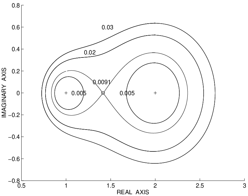
Example 6 The spectrum of the
quadratic matrix polynomial
is . Both eigenvalues are plotted as
“+” in Figure 4, and have algebraic multiplicity
equal to and geometric multiplicity equal to . The
boundaries for (i.e., for
perturbations measured in the absolute sense) and for are also sketched in
Figure 4.
Assuming that the pseudospectrum is
connected with one self-intersection plotted as “o”,
this figure indicates that consists of two connected
components for and that it is connected for
. Moreover, the singular values of the matrix
are and
i.e., is simple ( is not a fault point of
) and the function
has zero gradient at the point . Thus, by Proposition
17 and Theorem 18, two
perturbations of on the boundary of that have as a defective eigenvalue are
and in (18)
and (19), and can be easily constructed.
Figure 4: A single intersection point.
Left and right singular vectors of corresponding to
are
respectively, and left and right singular vectors of
corresponding to are
respectively.
The unitary matrix
satisfies
and the rank one matrix
satisfies
We define the matrices
and the matrices
all with spectral norm . Then the perturbations
and
lie on and have a multiple
eigenvalue (approximately) equal to with
algebraic multiplicity and geometric multiplicity ,
confirming our results.
It is important to note that, by Theorems 18 and
19, pseudospectra yield a visual approximation of the
distance to multiple eigenvalues, i.e., the spectral norm distance
from an matrix polynomial with a
nonsingular leading coefficient and all its eigenvalues simple to
matrix polynomials with multiple eigenvalues. For a given weight
function , this distance is defined by
Then Theorems 18 and 19 imply the
following result (see [3, 14] for the standard eigenvalue
problem).
Corollary 20
Let be an matrix polynomial as in
(1) with a nonsingular leading coefficient
and simple eigenvalues only.
(a)
If is bounded, then
(b)
If is unbounded and, as increases from
zero, its connected components meet at points different from the
origin, then
Example 7 Consider the
self-adjoint matrix polynomial
(see [13, Example 5.2]), which corresponds to a damped
vibrating system. The boundaries of for (i.e., for
perturbations measured in a relative sense) and for are drawn in Figure 5. The
eigenvalues of , and are plotted as “+”.
Figure 5: A damped vibrating system.
We learn from this figure and the above discussion that there
exist an in
(for which, the pseudospectrum starts having less than six
connected components) and an in (for
which, the pseudospectrum becomes connected) such that the
following hold:
1.
For every all the perturbations
have
only simple eigenvalues.
2.
For every
some perturbations
have multiple non-real eigenvalues (in a neighbourhood between
the eigenvalues of in the open upper half-plane and
in a neighbourhood between the eigenvalues of in the open
lower half-plane), but no perturbation in
has multiple real eigenvalues.
3.
For every some perturbations
have multiple real eigenvalues in the interval
.
Acknowledgements
The work of Peter Lancaster was supported in part by a grant from
the Natural Sciences and Engineering Research Council of Canada.
The work of Lyonell Boulton was supported in part by the Leverhulme Trust.
References
[1]
[2]
L.V. Ahlfors, Complex Analysis, McGraw Hill,
New York (1953).
[3]
R. Alam and S. Bora, On sensitivity of eigenvalues and
eigendecompositions of matrices, Linear Algebra Appl.,
396 (2005) 273-301.
[4]
L. Boulton, Non-variational approximation of discrete eigenvalues
of self-adjoint operators, to appear in IMA J. Numer. Anal.
(2006).
[5]
S. Boyd and C.A. Desoer, Subharmonic functions and performance
bounds on linear time-invariant feedback systems, IMA J.
Math. Control Inform., 2 (1985) 153-170.
[6]
E. Brieskorn and H. Knörrer, Plane Algebraic Curves,
Birkhäuser Verlag, Basel (1986).
[7]
E.B. Davies, Spectral enclosures and complex resonances for
general self-adjoint operators, LMS J. Comput. Math.,
1 (1998) 42-74.
[8]
J. Demmel, A counterexample for two conjectures about stability,
IEEE Trans. Auto. Control, AC-32 (1987) 340-342.
[9]
E. Gallestey, Computing spectral value sets using the
subharmonicity of the norm of rational matrices, BIT,
38 (1998) 22-33.
[10]
I. Gohberg, L. Rodman, and P. Lancaster, Matrix Polynomials,
Academic Press, Orlando, (1982).
[11] T. Kato, Perturbation Theory for Linear Operators,
Springer Verlag, New York (1980).
[12] K. Kendig, Elementary Algebraic Geometry,
Springer Verlag, New York (1977).
[13]
P. Lancaster and P. Psarrakos, On the pseudospectra of matrix
polynomials, SIAM J. Matrix Anal. Appl., 27
(2005) 115-129.
[14]
A.N. Malyshev, A formula for the 2-norm distance from a matrix to
the set of matrices with multiple eigenvalues, Numer.
Math., 83 (1999) 443-454.
[15]
R.G. Mosier, Root neighbourhoods of a polynomial, Math.
Comp., 47 (1986) 265-273.
[16]
J.-G. Sun, A note on simple non-zero singular values, J.
Comput. Math., 6 (1988) 258-266.
[17]
F. Tisseur, Backward error and condition of polynomial eigenvalue
problems, Linear Algebra Appl., 309 (2000)
339-361.
[18]
F. Tisseur and N.J. Higham, Structured pseudospectra for
polynomial eigenvalue problems with applications, SIAM J.
Matrix Anal. Appl., 23 (2001) 187-208.