A mirror construction for the totally nonnegative part of the Peterson varietyThanks: The author was supported by a Royal Society Dorothy Hodgkin Research Fellowship. This work was additionally supported by FWF Project P 17108.

Konstanze Rietsch Address: King’s College London, UK Email address: konstanze.rietsch@kcl.ac.uk Dedicated to Professor George Lusztig on his 60th birthday

Abstract.

We explain how A. Givental’s mirror symmetric family [14] to the type $A$ flag variety and its proposed generalization [3] to partial flag varieties by Batyrev, Ciocan-Fontanine, Kim and van Straten relate to the Peterson variety $Y\subset SL_{n}/B$ . We then use this theory to describe the totally nonnegative part of $Y$ , extending a result from [30].

Key words and phrases:

Flag varieties, quantum cohomology, mirror symmetry, total positivity

2000 Mathematics Subject Classification

20G20, 15A48, 14N35, 14N15

1. Introduction

The (type $A$ ) Peterson variety is a remarkable $(n-1)$ -dimensional projective subvariety of the full flag variety $SL_{n}/B$ used by Dale Peterson to construct all of the small quantum cohomology rings of the partial flag varieties $SL_{n}/P$ . This paper has two aims: firstly to relate the mirror symmetry constructions of Givental [14] and Batyrev, Ciocan-Fontanine, Kim, and van Straten [3] to the Peterson variety, and secondly to use these constructions to describe the totally nonnegative part of the Peterson variety.

The mirror constructions of [14] and [3] provide in the full flag variety case, and provide conjecturally in the partial flag variety case, a set of solutions to the quantum cohomology $D$ -module – a system of differential equations introduced by Givental whose total symbols recover relations of the small quantum cohomology ring [13] – in terms of oscillating integrals along families of cycles lying in a ‘mirror family’. These mirror families are $k$ -dimensional families $Z\to\mathbb{C}^{k}$ of affine varieties of the same dimension as $SL_{n}/P$ which are defined in terms of an associated graph, see Figure 1, and which come with natural volume forms on the fibers and a phase function $\mathcal{F}:Z\to\mathbb{C}$ . Here $k=\dim H^{2}(SL_{n}/P)$ . If the mirror conjecture holds then critical points of the phase function $\mathcal{F}$ along individual mirrors should relate to elements in the spectrum of the quantum cohomology ring, where fixing a variety in the mirror family corresponds to fixing the values of the quantum parameters $q_{1},\dotsc,q_{k}$ in $qH^{*}(SL_{n}/P)$ .

In Dale Peterson’s theory the spectrum of $qH^{*}(SL_{n}/P)$ is precisely a stratum $Y_{P}$ of the Peterson variety $Y$ . In this paper we compare Peterson’s $Y_{P}$ with the variety $Z^{crit}$ swept out by the critical points of $\mathcal{F}$ along the fibers of the mirror family $Z$ from [3, 14]. As it turns out $Z^{crit}$ recovers the parts of the Peterson variety that lie in certain Deodhar strata (a finer decomposition of the flag variety than the Bruhat decomposition). If $P=B$ then this includes an open dense subset of $Y_{B}$ . But in the case $P\neq B$ , the variety $Y_{P}$ can have entire irreducible components which lie in the ‘wrong’ Deodhar stratum and hence are not seen by $Z$ . This phenomenon is demonstrated explicitly in Section 9 for $SL_{4}/P=Gr_{2}(\mathbb{C}^{4})$ .

In this special case, $Gr_{2}(\mathbb{C}^{4})$ , an earlier mirror construction consistent with the ‘GBCKS’ mirror construction from [14, 3] was given by Eguchi, Hori and Xiong in [9, Appendix B], see [2]. Its deficiency with regard to recovering the quantum cohomology ring was observed also in [9], where it was fixed in an ad hoc way by a partial compactification. For a ‘fix’ of the GBCKS construction for general $SL_{n}/P$ we refer to our sequel paper [26]. It has not been checked how in the case of $Gr_{2}(\mathbb{C}^{4})$ the general construction of [26] relates to the ad hoc construction from [9].

Next we turn our attention to total positivity. The totally nonnegative part $(SL_{n}/B)_{\geq 0}$ of the flag variety was defined by Lusztig [21] as an extension of the classical theory of total positivity for matrices. It is a semi-algebraic subset inside the real flag variety $SL_{n}(\mathbb{R})/B$ (which we view with its Hausdorff topology).

In [30] we showed that the totally positive part of $Y_{P}$ (that is, the open interior of $Y_{P}\cap(SL_{n}/B)_{\geq 0}$ ) agrees with the subset of $Y_{P}$ where all of the Schubert classes take positive real values. Using this result it was then proved that the quantum parameters restrict to give a homeomorphism $Y_{P,>0}\overset{\sim}{\longrightarrow}\mathbb{R}_{>0}^{k},$ where $k=\dim Y_{P}$ , making $Y_{P,>0}$ a cell.

In Section 10 we use the mirror constructions from the previous sections to give a direct new proof of the above parameterization. In fact we can extend the result to the boundary to get a homeomorphism,

Y_{P,\geq 0}\overset{\sim}{\longrightarrow}\mathbb{R}_{\geq 0}^{k},

parameterizing the totally nonnegative part of $Y_{P}$ . Therefore we obtain a cell decomposition of the whole totally nonnegative part of the Peterson variety $Y$ . This mirror symmetric approach to proving the cell decomposition has the advantage of being completely elementary, whereas the proof in [30] relied on positivity of the structure constants of the quantum cohomology rings involved (the 3-point genus zero Gromov-Witten invariants for $SL_{n}/P$ ). On the other hand, though, we obtain no results about positivity of Schubert classes using only the mirror construction.

Finally, it is shown that the totally nonnegative part $Y_{\geq 0}$ of the Peterson variety is contractible. We conjecture that $Y_{\geq 0}$ , as a cell decomposed space, is homeomorphic to an $(n-1)$ -dimensional cube.

The interpretation of the GBCKS mirror construction and resulting proof of the cell decomposition of the totally nonnegative part of the Peterson variety $Y$ presented here date back to 2002, and were presented at the Erwin Schroedinger Institute in January of 2003 as well as alluded to in a footnote in [29]. In the full flag variety case a similar interpretation (but very different application) of Givental’s mirror coordinates has since appeared also in the interesting work of Gerasimov, Kharchev, Lebedev and Oblezin [12] on the quantum Toda lattice.

Acknowledgements : I would particularly like to thank George Lusztig and Dale Peterson. The first for introducing me to the marvelous theory of total positivity, and the second for his inspiring lectures on quantum cohomology. Without either one of them this paper would not have been written. These results were mostly written up while on leave in Waterloo, Canada. I thank the University of Waterloo for its hospitality.

2. Notation

From now on we let $n$ be the rank. Consider $G=SL_{n+1}(\mathbb{C})$ with fixed Borel subgroups $B=B^{+}$ , the group of upper-triangular matrices, and $B^{-}$ the lower-triangular matrices, and with maximal torus $T=B^{+}\cap B^{-}$ . We also have $U^{+}$ and $U^{-}$ , the unipotent radicals of $B^{+}$ and $B^{-}$ , respectively. Let $I=\{1,\dotsc,n\}$ and $e_{i},f_{i}$ the usual Chevalley generators of the Lie algebra $\mathfrak{g}=\mathfrak{sl}_{n+1}$ . So $e_{i}$ is the matrix with $1$ in position $(i,i+1)$ and $0$ everywhere else, and $f_{i}$ is its transpose. Let

x_{i}(t):=\exp(te_{i}),\quad y_{i}(t):=\exp(tf_{i}),\quad t\in\mathbb{C}

be the associated simple root subgroups. The datum $(T,B^{+},B^{-},x_{i},y_{i};i\in I)$ is called a pinning by Lusztig [21].

The Weyl group $W=N_{G}(T)/T$ is isomorphic to the symmetric group $S_{n+1}$ . Define representatives

\dot{s}_{i}:=y_{i}(-1)x_{i}(1)y_{i}(-1),\quad i\in I.

for the simple reflections $s_{i}:=\dot{s}_{i}T$ . The $s_{i}$ are Coxeter generators for $W$ . For general $w\in W$ a representative $\dot{w}\in G$ can be defined by $\dot{w}=\dot{s}_{i_{1}}\dot{s}_{i_{2}}\cdots\dot{s}_{i_{m}}$ , where $s_{i_{1}}s_{i_{2}}\cdots s_{i_{m}}$ is a (any) reduced expression for $w$ . The length $m$ of a reduced expression for $w$ is denoted by $\ell(w)$ .

Let $P\supseteq B$ be a parabolic subgroup of $G$ . Then there is a corresponding parabolic subgroup $W_{P}$ of $W$ generated by the elements $s_{i}$ with $\dot{s}_{i}\in P$ . Define $I_{P}=\{i\in I\ |\ \dot{s}_{i}\in P\}$ and $I^{P}$ its complement in $I$ . We have

	$\displaystyle W_{P}$	$\displaystyle=\left<s_{i}\ \|\ i\in I_{P}\right>,$
	$\displaystyle W^{P}$	$\displaystyle:=\{w\in W\ \|\ \ell(ws_{i})>\ell(w)\text{ for all $i\in I_{P}$}.\}$

The longest element in $W_{P}$ is denoted by $w_{P}$ . The longest element in $W$ is also denoted $w_{0}$ .

Let $I^{P}=\{n_{1},\dotsc,n_{k}\}$ where $0=n_{0}<n_{1}<n_{2}<\cdots<n_{k}<n+1=n_{k+1}$ . Then the homogeneous space $G/P$ can be identified with the variety of partial flags

\mathcal{F}_{n_{1},n_{2},\dotsc,n_{k}}(\mathbb{C}^{n+1})=\{\,\{0\}\subset V_{1}\subset V_{2}\subset\dots\subset V_{k}\subset\mathbb{C}^{n+1}\,|\,\dim_{\mathbb{C}}(V_{j})=n_{j}\,\}.

3. Quantum cohomology of $SL_{n+1}/P$

Let $H^{*}(G/P):=\bigoplus_{k}H^{2k}(G/P)$ be the cohomology of $G/P$ viewed as a graded vector space with grading given by $k$ . We will always take coefficients in $\mathbb{C}$ . For $w\in W^{P}$ denote by $\sigma^{w}_{P}$ the Poincaré dual class to the Schubert cycle $[X_{w}]$ where $X_{w}=\overline{B^{-}wP/P}$ . It is well known that the Schubert classes $\sigma^{w}_{P}$ are a homogeneous basis of $H^{*}(G/P)$ with $\deg(\sigma_{P}^{w})=\ell(w)$ .

The small quantum cohomology ring of the partial flag variety $SL_{n+1}/P$ has been described in the papers [1, 6, 18]. As a graded vector space it is given by

qH^{*}(SL_{n+1}/P)=H^{*}(SL_{n+1}/P)\otimes\mathbb{C}[q_{1}^{P},\dotsc,q_{k}^{P}],

where $\mathbb{C}[q_{1}^{P},\dotsc,q_{k}^{P}]$ is a graded polynomial ring with $\deg(q^{P}_{j})=n_{j+1}-n_{j-1}$ . The multiplicative structure constants are $3$ -point genus $0$ Gromov-Witten invariants, see for example [15, 6, 10, 19] or [7, 24]. For the purposes of this paper we will be mainly interested in presentations of these rings.

3.1.

Let

\mathbb{C}[\mathfrak{h}]=Sym^{\bullet}(\mathfrak{h}^{*})=\mathbb{C}[x_{1},\dotsc,x_{n+1}]/(x_{1}+\dotsc+x_{n+1})

be the coordinate ring of $\mathfrak{h}=Lie(T)$ , where the $x_{i}$ are the coordinates corresponding to the matrix entries along the diagonal. The $\mathbb{Z}$ -span of the $x_{i}$ is the character lattice $X^{*}(T)$ inside $\mathfrak{h}^{*}$ . The assignment taking a character $\lambda$ to the first Chern class of the associated line bundle $\mathcal{L}_{\lambda}=G\times_{B}\mathbb{C}_{\lambda}$ on $G/B$ , extends to a ring homomorphism $\mathbb{C}[\mathfrak{h}]\to H^{*}(G/B)$ . By Borel [4], this map identifies $H^{*}(G/B)$ with the quotient

\mathbb{C}[x_{1},\dotsc,x_{n+1}]/(e_{1}^{(n+1)},\dotsc,e_{n+1}^{(n+1)}),

where $e_{l}^{(n+1)}=e_{l}(x_{1},\dotsc,x_{n+1})$ is the $l$ -th elementary symmetric polynomial in $n+1$ variables. Moreover the projection $G/B\to G/P$ gives rise to an inclusion $H^{*}(G/P)\to H^{*}(G/B)$ which identifies $H^{*}(G/P)$ with the $W_{P}$ -invariant part of $H^{*}(G/B)$ . Explicitly, consider the ring $\mathbb{C}[x_{1},\dotsc,x_{n+1}]^{W_{P}}$ , which is a polynomial ring generated by the elementary symmetric polynomials

		$\displaystyle\sigma^{(1)}_{l}:=e_{l}(x_{1},\dotsc,x_{n_{1}}),$	$\displaystyle\qquad l=1,\dotsc,n_{1},$
		$\displaystyle\sigma^{(2)}_{l}:=e_{l}(x_{n_{1}+1},\dotsc,x_{n_{2}}),$	$\displaystyle\qquad l=1,\dotsc,n_{2}-n_{1},$
		$\displaystyle\qquad\qquad\vdots$
		$\displaystyle\sigma^{(k+1)}_{l}:=e_{l}(x_{n_{k}+1},\dotsc,x_{n+1}),$	$\displaystyle\qquad l=1,\dotsc,n+1-n_{k}.$

The full elementary symmetric polynomials $e_{r}^{(n+1)}$ may be expressed as polynomials in the $\sigma^{(j)}_{l}$ and we let $J$ denote the ideal these polynomials generate. Then we have

(3.1)

H^{*}(G/P)\cong\mathbb{C}[\sigma^{(1)}_{1},\sigma^{(1)}_{2},\dotsc,\sigma^{(k+1)}_{n+1-n_{k}}]/J.

3.2.

The analogous presentation of the quantum cohomology ring due to [1, 6, 18] goes as follows. From now on let us write $\sigma^{(j)}_{l}$ for the element $\sigma^{(j)}_{l}\otimes 1\in qH^{*}(G/P)$ , and similarly $q_{j}^{P}$ or just $q_{j}$ for $1\otimes q_{j}^{P}$ . These are the generators.

Definition 3.1 ( $(\mathbf{q},P)$ -elementary symmetric polynomials).

Let $l\in\mathbb{Z}$ and $j\in\{-1,0,\dotsc,k+1\}$ . Define elements $E^{(j)}_{l,P}=E^{(j)}_{l}\in\mathbb{C}[\sigma^{(1)}_{1},\dotsc,\sigma^{(k+1)}_{n+1-n_{k}}\,,\,q_{1},\dotsc,q_{k}]$ recursively as follows. The initial values are

E^{(-1)}_{l}=E^{(0)}_{l}=0\ \text{ for all $l$},\ \ \text{and }\ E^{(j)}_{l}=0\ \text{ unless }0\leq l\leq n_{j},

and we set $\sigma^{(j)}_{l}=0$ if $l>n_{j}-n_{j-1}$ and $\sigma^{(j)}_{0}=1$ for all $j$ . For $1\leq j\leq k+1$ and $0\leq l\leq n_{l}$ the polynomial $E^{(j)}_{l}$ satisfies

E^{(j)}_{l}\hskip-2.84544pt=\hskip-2.84544pt\left(E^{(j-1)}_{l}+\sigma^{(j)}_{1}E^{(j-1)}_{l-1}+\cdots+\sigma^{(j)}_{l-1}E^{(j-1)}_{1}+\sigma^{(j)}_{l}\right)\\ +(-1)^{n_{j}-n_{j-1}+1}q_{j-1}E^{(j-2)}_{l-n_{j}+n_{j-2}}.

Theorem 3.2 ([1, 18, 6]).

The quantum cohomology ring $qH^{*}(G/P)$ is given by the generators $\sigma^{(1)}_{1},\dotsc,\sigma^{(k+1)}_{n+1-n_{k}},q_{1},\dots,q_{k}$ with relations

E^{(k+1)}_{1}=E^{(k+1)}_{2}=\cdots=E^{(k+1)}_{n+1}=0.

4. The Peterson variety

Dale Peterson [25] discovered a remarkable unified construction for all of the quantum cohomology rings $qH^{*}(G/P)$ , for varying $P$ , as coordinate rings of the strata of a single projective variety $Y$ . For $G$ of general type this ‘Peterson variety’ $Y$ is a subvariety of the Langlands dual flag variety $G^{\vee}/B^{\vee}$ . We will recall his result in type $A$ .

4.1.

In our conventions the Peterson variety will be a subvariety of $G/B^{-}$ , where $G=SL_{n+1}(\mathbb{C})$ . Let us recall first the Bruhat and opposite Bruhat decompositions

G/B^{-}=\bigsqcup_{w\in W}B^{-}\dot{w}B^{-}/B^{-}=\bigsqcup_{v\in W}B^{+}\dot{v}B^{-}/B^{-}.

We also define

\mathcal{R}_{v,w}:=B^{+}\dot{v}B^{-}\cap B^{-}\dot{w}B^{-}/B^{-}.

This intersection of opposed Bruhat cells is smooth of pure dimension $\ell(w)-\ell(v)$ if $v\leq w$ in the Bruhat order, and otherwise empty, see [17, 22].

Let $\{\omega_{i}\ |\ i\in I\}$ be the set of fundamental weights. Consider $V^{\omega_{r}}=\bigwedge^{r}\mathbb{C}^{n+1}$ , the $r$ -th fundamental representation of $G$ with its standard basis $\{v_{i_{1}}\wedge\cdots\wedge v_{i_{r}}\,|\,1\leq i_{1}<i_{2}\cdots<i_{r}\leq n+1\}$ . The stabilizer of the highest weight space $\left<v_{1}\wedge\cdots\wedge v_{r}\right>_{\mathbb{C}}$ defines a maximal parabolic which we denote $P_{\omega_{r}}$ . Let us write $V_{-\omega_{r}}$ for $V^{\omega_{n-r+1}}$ , which is the representation with lowest weight $-\omega_{r}$ , and fix the lowest weight vector $v_{-\omega_{r}}=v_{r+1}\wedge\cdots\wedge v_{n+1}$ . For $w\in W^{P_{\omega_{r}}}$ we have a well defined rational function

(4.1)

M_{w\omega_{r}}(gB^{-}):=\frac{\left<g\cdot v_{-\omega_{r}},\dot{w}\cdot v_{-\omega_{r}}\right>}{\left<g\cdot v_{-\omega_{r}},v_{-\omega_{r}}\right>}

on the flag variety $G/B^{-}$ , where $\left<\ ,\ \right>$ denotes the inner product on $V_{-\omega_{r}}$ such that the standard basis is orthonormal.

Let us introduce the principal nilpotent element

f=f_{1}+\dotsc+f_{n}.

We write $g\cdot X:=gXg^{-1}$ for the adjoint action of $g\in G$ on $X\in\mathfrak{g}$ .

Definition 4.1 (The Peterson variety).

Let $Y\subset G/B^{-}$ be the projective variety defined by

Y:=\left\{gB^{-}\,\left|\,g^{-1}\cdot f\in\mathfrak{b}^{-}\oplus\sum_{i\in I}\mathbb{C}e_{i}\right.\right\}.

More formally, $Y$ is defined by the equations

{pr}_{\mathfrak{g}_{\alpha}}(g^{-1}\cdot f)=0,

where ${pr}_{\mathfrak{g}_{\alpha}}$ is the projection onto the weight space $\mathfrak{g}_{\alpha}$ , and $\alpha$ runs through the set of all roots which are positive but not simple. For a parabolic $P\supseteq B$ define the (non-reduced) intersection

Y_{P}:=Y\times_{G/B^{-}}B^{+}\dot{w}_{P}B^{-}/B^{-}.

Suppose $P^{\prime}\supseteq P$ is another parabolic. Then we set

Y_{(P,P^{\prime})}:=Y\times_{G/B^{-}}\mathcal{R}_{w_{P},w_{P^{\prime}}}.

We also write $Y_{P}^{\circ}$ for $Y_{(P,G)}$ .

The Peterson variety and some generalized versions of it are also of independent interest and have been studied in the papers [5, 19, 20, 32].

4.2.

We now state Peterson’s result in type $A$ , see also [19] and [30, 31].

Theorem 4.2 (Peterson [25]).

(1)

The $\mathbb{C}$ -valued points of $Y$ decompose into a union of strata,

$Y(\mathbb{C})=\bigsqcup_{P\supseteq B}Y_{P}(\mathbb{C}).$
(2)

Let $w^{[r]}_{l}=s_{r-l+1}s_{r-l+2}\cdots s_{r-1}s_{r}$ , where $1\leq l\leq r$ . For each parabolic $P$ there is a unique isomorphism

$\psi_{P}:\mathbb{C}[Y_{P}]\overset{\sim}{\longrightarrow}qH^{*}(G/P),$

such that $M_{w^{[n_{j}]}_{l}\omega_{n_{j}}}\mapsto E^{(j)}_{l}$ for $j=1,\dotsc,k$ and $1\leq l\leq n_{j}$ .
(3)

$\psi_{P}$ induces an isomorphism

$\psi_{P}^{\circ}:\mathbb{C}[Y_{P}^{\circ}]\overset{\sim}{\longrightarrow}qH^{*}(G/P)[q_{1}^{-1},\dotsc,q_{k}^{-1}].$

Note that $M_{w^{[r]}_{l}\omega_{r}}$ is a regular function on the Bruhat cell $B^{+}\dot{w}_{P}B^{-}/B^{-}$ if $r\in I^{P}$ and $1\leq l\leq r$ .

5. The GBKCS mirror construction for $SL_{n+1}/P$

In [14], A. Givental introduced a mirror family to the full flag variety $SL_{n+1}/B$ and proved a kind of mirror theorem. His mirror construction was generalized by Batyrev, Kim, Ciocan-Fontanine and van Straten in [3], who defined a similar family associated to partial flag varieties $SL_{n+1}/P$ and conjectured the analogous mirror theorem. We recall their construction, which we will refer to as the GBCKS construction, here.

5.1.

Let us fix the partial flag variety

SL_{n+1}/P=\mathcal{F}_{n_{1},\dotsc,n_{k}}(\mathbb{C}^{n+1}).

As before $n_{k+1}=n+1$ and $n_{0}=0$ . Define an oriented graph $(\mathcal{V},\mathcal{A})=(\mathcal{V}^{P},\mathcal{A}^{P})$ as follows. Let the vertex set $\mathcal{V}^{P}\subset\mathbb{Z}^{2}$ be defined by $\mathcal{V}^{P}=\mathcal{V}^{P}_{\star}\sqcup\mathcal{V}^{P}_{\bullet}$ where

	$\displaystyle\mathcal{V}^{P}_{\bullet}$	$\displaystyle=\{(m,r)\in\mathbb{Z}_{\geq 0}^{2}\ \|\ n_{1}\leq m\leq n,\text{ and $1\leq r\leq n_{j}$ if $m<n_{j+1}$, for $j=1,\dotsc,k$}\},$
	$\displaystyle\mathcal{V}^{P}_{\star}$	$\displaystyle=\{\star_{j}=(n_{j}-1,n_{j-1}+1)\ \|\ j=1,\dotsc,k+1\}.$

Consider $v=({v_{1}},{v_{2}})$ in $\mathcal{V}^{P}$ . If $v^{\prime}:=(v_{1},v_{2}-1)$ is in $\mathcal{V}^{P}$ then there is a horizontal arrow, denoted $d_{v}$ or $d_{v_{1},v_{2}}$ , pointing from $v$ to $v^{\prime}$ . If $v^{\prime\prime}=(v_{1}-1,v_{2})$ is in $\mathcal{V}^{P}$ then there is a vertical arrow $c_{v}$ , or $c_{v_{1},v_{2}}$ , going from $v$ to $v^{\prime\prime}$ . We define $\mathcal{A}^{P}$ to be the set of all such arrows.

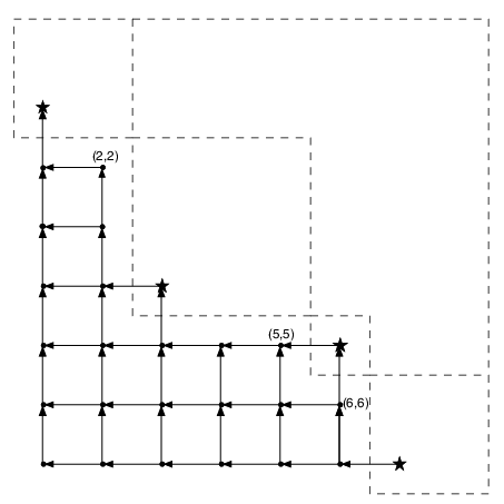
See Figure 1 for an example of a graph $(\mathcal{V}^{P},\mathcal{A}^{P})$ . The vertices are arranged like entries in a matrix, with a vertex $(i,j)$ positioned in the $i$ -th row and $j$ -th column. The dotted lines indicate the shape of the parabolic subgroup $P$ in question. And the vertices in $\mathcal{V}^{P}_{\star}$ and $\mathcal{V}^{P}_{\bullet}$ are represented by stars and dots, respectively.

As the parabolic will be fixed most of the time we may omit the superscript $P$ and write $\mathcal{V}$ for $\mathcal{V}^{P}$ and $\mathcal{A}$ for $\mathcal{A}^{P}$ .

Refer to caption — Figure 1. The graph for $G/P=\mathcal{F}_{2,5,6}(\mathbb{C}^{8})$

5.2.

Let

Z=Z_{P}:=\left\{\rho=(\rho_{a})_{a\in\mathcal{A}}\in\mathbb{C}^{\mathcal{A}}\ \left|\ \rho_{c}\rho_{d}=\rho_{d^{\prime}}\rho_{c^{\prime}},\ \begin{array}[]{l}\text{whenever $c,c^{\prime},d,d^{\prime}$ form }\\ \text{a square, \eqref{e:box}, in the graph}\end{array}\right.\right\}.

(5.1)

\begin{matrix}\bullet&\overset{d}{\longleftarrow}&\hskip-8.5359pt\bullet\\ \hskip-8.5359ptc^{\prime}\uparrow&&\uparrow c\\ \bullet&\overset{d^{\prime}}{\longleftarrow}&\hskip-8.5359pt\bullet\end{matrix}

The upper right hand corner vertex in (5.1) may of course lie in $\mathcal{V}_{\star}$ .

For simplicity of notation we identify the arrows with functions on $Z$ via

a:\rho\mapsto\rho_{a}.

The coordinate ring $\mathbb{C}[Z]$ can be viewed as the affine algebra over $\mathbb{C}$ with generators $a\in\mathcal{A}$ and relations $cd=d^{\prime}c^{\prime}$ for $c,d,c^{\prime},d^{\prime}\in\mathcal{A}$ arranged as in (5.1). We will refer to these as ‘box relations’. There is a grading on $\mathbb{C}[Z]$ given by setting $deg(a)=1$ for every generator $a\in\mathcal{A}$ .

5.3.

The coordinate ring $\mathbb{C}[Z]$ has some special elements which we define below. For $j=1,\dotsc k$ let $\tilde{q}_{j}$ be a product of generators represented by the arrows along a path from vertex $\star_{j+1}$ to $\star_{j}$ . Explicitly,

\tilde{q}_{j}=d_{n_{j+1}-1,n_{j+1}}\left(\prod_{i=1}^{n_{j+1}-n_{j}-1}c_{n_{j}+i,n_{j}}\right)\left(\prod_{i=1}^{n_{j}-n_{j-1}-1}d_{n_{j},n_{j-1}+i+1}\right)c_{n_{j},n_{j-1}+1},

where we have chosen the path along the outer rim. Note that $deg(\tilde{q}_{j})=n_{j+1}-n_{j-1}$ . Now $Z$ is viewed as a family of varieties via

(5.2)

\tilde{q}=(\tilde{q}_{1},\dots,\tilde{q}_{k}):Z\longrightarrow\mathbb{C}^{k}.

The fiber over $\tilde{Q}\in\mathbb{C}^{k}$ is denoted by $Z_{\tilde{Q}}$ .

5.4.

Finally [14, 3] introduce a function

\mathcal{F}=\sum_{a\in\mathcal{A}}a

on $Z$ . This is the phase function of the proposed mirror model, see Section 6. We will study its critical point sets along the fibers of the family $Z$ in Section 7.

5.5.

Define

(5.3)

Z^{\circ}=Z^{\circ}_{P}:=\left\{\rho\in Z\ |\ \rho_{a}\neq 0,\ \text{all $a\in\mathcal{A}$}\right\}=\left\{\rho\in Z\ |\ \tilde{q}_{j}(\rho)\neq 0,\ 1\leq j\leq k\right\}.

Let the map (5.2) restricted to $Z^{\circ}$ be again denoted by $\tilde{q}$ ,

\tilde{q}=(\tilde{q}_{1},\dots,\tilde{q}_{k}):Z^{\circ}\longrightarrow(\mathbb{C}^{*})^{k}.

This restricted map is a trivial bundle with fiber isomorphic to $(\mathbb{C}^{*})^{\mathcal{V}_{\bullet}}$ .

As in [14] one can choose an explicit trivialization by introducing vertex variables $(t_{v})_{v\in\mathcal{V}}$ running through $\mathbb{C}^{*}$ . For any arrow $a$ denote by $h(a)$ and $t(a)\in\mathcal{V}$ the head and tail of $a$ . Then $(t_{v})_{v\in\mathcal{V}}\mapsto\rho=(t_{h(a)}t_{t(a)}^{-1})_{a\in\mathcal{A}}$ defines a map

(5.4)

(\mathbb{C}^{*})^{\mathcal{V}}\longrightarrow Z^{\circ}.

This map descends to the quotient by the diagonal action of $\mathbb{C}^{*}$ to give an isomorphism $(\mathbb{C}^{*})^{\mathcal{V}}/\mathbb{C}^{*}\overset{\sim}{\longrightarrow}Z^{\circ}$ .

Moreover, for given $\tilde{Q}=(\tilde{Q}_{1},\dotsc,\tilde{Q}_{k})\in(\mathbb{C}^{*})^{k}$ , the map obtained from (5.4) after fixing the $t_{\star_{j}}$ (uniquely up to a common scalar multiple) such that $t_{\star_{j}}t_{\star_{j+1}}^{-1}=\tilde{Q}_{j}$ gives rise to an isomorphism

(\mathbb{C}^{*})^{\mathcal{V}_{\bullet}}\overset{\sim}{\longrightarrow}Z_{\tilde{Q}}.

Choosing $t_{\star_{j}}=\tilde{Q}_{j}\dotsc\tilde{Q}_{k}$ , say, and $t_{\star_{k+1}}=1$ gives rise to a global trivialization of $\tilde{q}:Z^{\circ}\to(\mathbb{C}^{*})^{k}$ .

5.6.

For a pair of parabolics $P^{\prime}\supseteq P$ containing $B$ the corresponding vertex sets are related by $\mathcal{V}^{P^{\prime}}_{\bullet}\subseteq\mathcal{V}^{P}_{\bullet}$ and we define

Z_{(P,P^{\prime})}:=\left\{\rho\in Z_{P}\ |\ \text{If $a\in\mathcal{A}^{P}$, then $a(\rho)=0$ $\iff$ $h(a)\in\mathcal{V}^{P^{\prime}}_{\bullet}$ or $t(a)\in\mathcal{V}^{P^{\prime}}_{\bullet}$}\right\}.

Note that if $P^{\prime}=G$ we have $Z_{(P,G)}=Z^{\circ}_{P}$ . In general

Z_{(P,P^{\prime})}\subset\{\rho\in Z_{P}\ |\ \text{$\tilde{q}_{j}(\rho)=0\iff n_{j}\in I^{P^{\prime}}$}\},

and the two sets are not equal. In particular $Z_{P}\neq\bigsqcup_{P^{\prime}\supseteq P}Z_{(P,P^{\prime})}$ , see for example Remark 7.3.

6. Mirror conjecture and quantum cohomology

The Givental/Eguchi-Hori-Xiong type mirror conjecture [3, Conjecture 5.5.1] associated to the data introduced in the previous section states that a full set of solutions to the quantum cohomology $D$ -module (e.g. [7, Chapter 10]) associated to $SL_{n+1}/P$ can be written down on the mirror side as complex oscillatory integrals of the form

S_{\Gamma}(s):=\int_{\Gamma_{s}}e^{\mathcal{F}/z}\omega_{s}.

Here $s=(s_{1},\dotsc,s_{k+1})\in\mathbb{C}^{k+1}$ . Furthermore $\omega_{s}$ is a particular volume form on $Z_{\tilde{Q}(s)}:=Z_{(e^{s_{1}-s_{2}},\dotsc,e^{s_{k}-s_{k+1}})}$ , and $\Gamma$ is a suitable family of (possibly non-compact) middle-dimensional cycles $\Gamma_{s}\subset Z_{\tilde{Q}(s)}$ for which the integral converges. In the $SL_{n+1}/B$ case this conjecture was proved by Givental [14].

Whenever the conjecture holds the variety swept out by the critical points of $\mathcal{F}$ along the fibers of $Z^{\circ}\to(\mathbb{C}^{*})^{k}$ should satisfy the relations of the small quantum cohomology ring (compare with [13]), or ideally completely recover the spectrum $Spec\left(qH^{*}(SL_{n+1}/P)[q_{1}^{-1},\dots,q_{k}^{-1}]\right)$ .

6.1.

Let

Z^{\circ,crit}=Z^{\circ,crit}_{P}:=\left\{\rho\in Z^{\circ}\ |\text{ $\mathcal{F}|_{Z_{\tilde{q}(\rho)}}$ has a critical point at $\rho$}\ \right\}.

Following [14] we write $\mathcal{F}$ in logarithmic vertex variables $T_{v}\in\mathbb{C}$ with $e^{T_{v}}=t_{v}$ to obtain

\frac{\partial}{\partial T_{v}}\mathcal{F}=\sum_{a,h_{a}=v}e^{T_{h(a)}-T_{t(a)}}-\sum_{a,t_{a}=v}e^{T_{h(a)}-T_{t(a)}}.

Therefore the critical point condition reads

(6.1)

\sum_{a,h(a)=v}a-\sum_{a,t(a)=v}a=0,\qquad\text{ for all $v\in\mathcal{V}_{\bullet}$.}

For every vertex in $\mathcal{V}_{\bullet}$ , the sum of incoming variables equals the sum of outgoing variables. We define

(6.2)

Z^{crit}=Z^{crit}_{P}:=\left\{\rho\in Z_{P}\ |\ \text{ $\rho$ satisfies \eqref{e:crit}}\right\}.

7. The GBCKS construction and the Peterson variety

In this section we demonstrate explicitly how the GBCKS construction relates to $qH^{*}(SL_{n+1}/P)$ . This is best done by comparing $Z^{crit}$ with the Peterson variety $Y_{P}$ . While in the full flag variety case $Z^{\circ,crit}$ is almost isomorphic to $Y_{B}^{\circ}$ , or $Spec(qH^{*}(SL_{n+1}/B)[q_{1}^{-1},\dotsc,q_{n}^{-1}])$ (it is isomorphic to an open dense subset), we will see that in the partial flag variety case entire irreducible components of $Y_{P}^{\circ}$ can be missed out by $Z^{\circ,crit}$ . Nevertheless our result, see in particular Proposition 8.3, should be considered as positive evidence for the mirror conjecture from [3]. Although, as it turns out, the GBCKS mirror family $Z$ , or rather $Z^{\circ}$ , may be thought of as an open subset of a more complete (and canonical) mirror family, see [26].

7.1.

We want to define a map $\phi:Z\to SL_{n+1}/B^{-}$ . Let us first introduce some new notation. Set

(7.1)

l_{j}:=n_{j}-n_{j-1},\quad\text{ for $j=1,\dotsc,k+1$.}

For $(m,r)\in\mathcal{V}_{\bullet}$ let

(7.2)

\tilde{c}_{m,r}=\begin{cases}c_{n_{j},n_{j-1}+1}\prod^{p}_{i=2}d_{n_{j},n_{j-1}+i}&\text{if $m=n_{j}$ and $r=n_{j-1}+p$,}\\ &\text{where $2\leq p\leq l_{j}$ and $j=1,\dotsc,k$,}\\ c_{m,r}&\text{otherwise.}\end{cases}

Note that $\deg(\tilde{c}_{n_{j},n_{j-1}+p})=p$ . We also define for later use

(7.3)

\tilde{d}_{m,r+1}=\begin{cases}d_{n_{j}-1,n_{j-1}+1}\prod_{i=1}^{p-1}c_{n_{j}-i,n_{j-1}}&\text{if $r=n_{j-1}$ and $m=n_{j}-p$,}\\ &\text{where $2\leq p\leq l_{j}$ and $j=1,\dotsc,k$,}\\ d_{m,r+1}&\text{otherwise.}\end{cases}

Note that $\tilde{q}_{j}=\tilde{c}_{n_{j},n_{j}}\tilde{d}_{n_{j},n_{j}+1}$ .

Consider the simple root subgroups $x_{i}(t)$ for $i\in I$ . Let us also fix a one-parameter subgroup associated to a positive root $\alpha_{[i,i^{\prime}]}:=\alpha_{i}+\alpha_{i+1}+\dotsc+\alpha_{i^{\prime}}$ with $1\leq i<i^{\prime}\leq n$ by defining

(7.4)

x_{[i,i^{\prime}]}(t):=\dot{s}_{i^{\prime}}\dot{s}_{i^{\prime}-1}\dotsc\dot{s}_{i+1}x_{i}(t)\dot{s}_{i+1}^{-1}\dotsc\dot{s}_{i^{\prime}-1}^{-1}\dot{s}_{i^{\prime}}^{-1}.

Explicitly, $x_{[i,i^{\prime}]}(t)$ is the unipotent upper-triangular matrix with $(i,i^{\prime}+1)$ -entry $t$ and zeros everywhere else above the diagonal.

Let $r=n_{j-1}+p$ for some $j=1,\dotsc,k$ and $1\leq p\leq l_{j}$ . We define elements $g_{r}$ in $SL_{n+1}(\mathbb{C}[Z])$ by

$\displaystyle g_{n_{j-1}+1}$	$\displaystyle=$	$\displaystyle x_{n}(c_{n,n_{j-1}+1})x_{n-1}(c_{n-1,n_{j-1}+1})\dotsc x_{n_{j}}(c_{n_{j},n_{j-1}+1})\dot{s}_{n_{j}-1}\dotsc\dot{s}_{n_{j-1}+1},$
$\displaystyle g_{r}$	$\displaystyle=$	$\displaystyle x_{n}(c_{n,r})x_{n-1}(c_{n-1,r})\dotsc\dotsc x_{n_{j}}(\tilde{c}_{n_{j},r})\dot{s}_{n_{j}-1}\dot{s}_{n_{j}-2}\dotsc\dot{s}_{n_{j-1}+p},$
$\displaystyle g_{n_{j}}$	$\displaystyle=$	$\displaystyle x_{n}(c_{n,n_{j}})x_{n-1}(c_{n-1,n_{j}})\dotsc x_{n_{j}}(\tilde{c}_{n_{j}+1,n_{j}}).$

The element $g_{r}$ should be viewed as associated to the $r$ -th column in the graph $(\mathcal{V},\mathcal{A})$ . For $r=n_{k}+p$ with $1\leq p\leq l_{k+1}-1$ set

\displaystyle g_{n_{k}+p}=\dot{s}_{n}\dot{s}_{n-1}\dotsc\dot{s}_{n_{k}+p}.

We can now form the product to get a new element $g:=g_{1}g_{2}\dots g_{n}\in SL_{n+1}(\mathbb{C}[Z])$ , or equivalently a map

g:Z\to SL_{n+1}(\mathbb{C}).

We define the map $\phi$ , or $\phi_{P}$ , keeping track of the dependence on $P$ , by

(7.5)

\begin{array}[]{llcl}\phi_{P}:&Z_{P}&\to&SL_{n+1}/B^{-},\\ &\rho&\mapsto&g(\rho)B^{-}.\end{array}

Note that the image of $\phi_{P}$ lies in $B^{+}\dot{w}_{P}B^{-}/B^{-}$ .

7.2. Deodhar strata

The intersections of opposite Bruhat cells $\mathcal{R}_{v,w}$ have a decomposition into finitely many strata (each of the form $\mathbb{C}^{l}\times(\mathbb{C}^{*})^{m}$ ) due to Deodhar [8]. We will not give Deodhar’s original definition here, but rather use an equivalent description from [23] which is ideally suited to our needs.

The Deodhar decomposition of $\mathcal{R}_{v,w}$ depends on a choice of reduced expression for the longer element, $w$ . We write $\mathbf{w}=s_{i_{1}}\dotsc s_{i_{m}}$ to mean $w$ with the given reduced expression $(i_{1},\dotsc,i_{m})$ . A sequence of integers $1\leq j_{1}<\dotsc<j_{l}\leq m$ gives rise to a subexpression $\mathbf{v}$ for $v$ in $\mathbf{w}$ if $s_{i_{j_{1}}}s_{i_{j_{2}}}\dotsc s_{i_{j_{l}}}=v$ . The latter need not be a reduced expression for $v$ . Associated to the pair $(\mathbf{v},\mathbf{w})$ of reduced expression $\mathbf{w}$ and subexpression $\mathbf{v}$ we have the sets

$\displaystyle J^{+}_{(\mathbf{v},\mathbf{w})}$	$\displaystyle=$	$\displaystyle\left\{r=j_{p}\ \|\ \text{some $p=1,\dotsc,l$ with $s_{j_{1}}\dotsc s_{j_{p-1}}>s_{j_{1}}\dotsc s_{j_{p-1}}s_{j_{p}}$ }\right\},$
$\displaystyle J^{-}_{(\mathbf{v},\mathbf{w})}$	$\displaystyle=$	$\displaystyle\left\{r=j_{p}\ \|\ \text{some $p=1,\dotsc,l$ with $s_{j_{1}}\dotsc s_{j_{p-1}}<s_{j_{1}}\dotsc s_{j_{p-1}}s_{j_{p}}$ }\right\},$
$\displaystyle J^{\circ}_{(\mathbf{v},\mathbf{w})}$	$\displaystyle=$	$\displaystyle\{1,\dotsc,m\}\setminus\{j_{1},\dotsc,j_{l}\}.$

The strata of $\mathcal{R}_{v,w}$ are indexed by certain subexpressions $\mathbf{v}$ for $v$ in $\mathbf{w}$ called distinguished, see [8] or [23, Section 3] for a definition. By [23, Proposition 5.2] the Deodhar stratum corresponding to $\mathbf{v},\mathbf{w}$ is given by

(7.6)

\mathcal{R}_{\mathbf{v},\mathbf{w}}=\left\{g_{1}g_{2}\dotsc g_{m}B_{-}\ \left|\ g_{r}=\begin{cases}\dot{s}_{i_{r}}&\text{if $r\in J^{+}_{(\mathbf{v},\mathbf{w})}$,}\\ y_{i_{r}}(m_{r})\dot{s}_{i_{r}}^{-1},\ \,m_{r}\in\mathbb{C},&\text{if $r\in J^{-}_{(\mathbf{v},\mathbf{w})}$},\\ x_{i_{r}}(t_{r}),\qquad\quad t_{r}\in\mathbb{C}^{*},&\text{if $r\in J^{\circ}_{(\mathbf{v},\mathbf{w})}$}\end{cases}\quad\right.\right\}.

Moreover the parameters $t_{r}\in\mathbb{C}^{*}$ and $m_{r}\in\mathbb{C}$ define an isomorphism

(\mathbb{C}^{*})^{J^{\circ}_{(\mathbf{v},\mathbf{w})}}\times\mathbb{C}^{J^{-}_{(\mathbf{v},\mathbf{w})}}\overset{\sim}{\longrightarrow}\mathcal{R}_{\mathbf{v},\mathbf{w}}.

There is a unique distinguished subexpression $\mathbf{v}^{+}$ of $\mathbf{w}$ with $J^{-}_{(\mathbf{v}^{+},\mathbf{w})}=\emptyset$ , which we call the positive subexpression for $v$ in $\mathbf{w}$ . It can be constructed as the rightmost reduced subexpression for $v$ in $\mathbf{w}$ , see for example [23, Lemma 3.5], and it corresponds to the unique open stratum $\mathcal{R}_{\mathbf{v}^{+},\mathbf{w}}$ in $\mathcal{R}_{v,w}$ .

7.3.

Consider the reduced expression $\mathbf{w_{0}}$ of $w_{0}$ given by

(s_{n}s_{n-1}\dotsc s_{1})(s_{n}s_{n-1}\dotsc s_{2})\cdots(s_{n}s_{n-1})s_{n}.

Let $P^{\prime}$ be a parabolic with $0\leq a_{1}<b_{1}<a_{2}<b_{2}<\dotsc<a_{h}<b_{h}\leq n$ such that

I_{P^{\prime}}=[a_{1}+1,b_{1}]\cup[a_{2}+1,b_{2}]\cup\cdots\cup[a_{h}+1,b_{h}],

as union of intervals in $\{1,\dotsc,n\}$ . We have a reduced expression $\mathbf{w_{P^{\prime}}}$ given by

		$\displaystyle(s_{b_{1}}s_{b_{1}-1}\dotsc s_{a_{1}+1})(s_{b_{1}}s_{b_{1}-1}\dotsc s_{a_{1}+2})\cdots(s_{b_{1}}s_{b_{1}-1})s_{b_{1}}$
		$\displaystyle(s_{b_{2}}s_{b_{2}-1}\dotsc s_{a_{2}+1})(s_{b_{2}}s_{b_{2}-1}\dotsc s_{a_{2}+2})\cdots(s_{b_{2}}s_{b_{2}-1})s_{b_{2}}$
		$\displaystyle\qquad\qquad\qquad\qquad\qquad\qquad\cdots$
		$\displaystyle(s_{b_{h}}s_{b_{h}-1}\dotsc s_{a_{h}+1})(s_{b_{h}}s_{b_{h}-1}\dotsc s_{a_{h}+2})\cdots(s_{b_{h}}s_{b_{h}-1})s_{b_{h}}.$

The expression $\mathbf{w_{P^{\prime}}}$ can also be constructed as the reduced expression obtained from the positive subexpression for $w_{P^{\prime}}$ in $\mathbf{w_{0}}$ .

Lemma and Definition 7.1.

Let $P^{\prime}$ be a parabolic subgroup with $P^{\prime}\supseteq P$ and recall the definition of $Z_{(P,P^{\prime})}$ from Section 5.6. The map $\phi_{P}:Z_{P}\to G/B^{-}$ from (7.5) restricts to

\phi_{(P,P^{\prime})}:Z_{(P,P^{\prime})}\longrightarrow\mathcal{R}_{\mathbf{w_{P}^{+}},\mathbf{w_{P^{\prime}}}}.

In particular setting $P^{\prime}=G$ gives $Z_{(P,G)}=Z^{\circ}_{P}$ and we define

\phi^{\circ}_{P}:=\phi_{(P,G)}:Z^{\circ}_{P}\longrightarrow\mathcal{R}_{\mathbf{w_{P}^{+}},\mathbf{w_{0}}}.

Proof of Lemma 7.1.

This lemma follows directly from the definitions of $Z_{(P,P^{\prime})}$ and the map $\phi_{P}$ together with the description of the Deodhar strata proved in [23, Proposition 5.2], see (7.6). ∎

We can now use $\phi_{P}$ to relate the GBCKS construction to the Peterson variety.

Theorem 7.2.

(1)

The map $\phi_{P}$ restricts to a map

\phi_{P}^{crit}:Z^{crit}_{P}\longrightarrow Y_{P}

such that the following diagram commutes,

\begin{matrix}Z^{crit}_{P}&\overset{\phi^{crit}_{P}}{\longrightarrow}&Y_{P}\\ \ \underset{\tilde{q}\ \ }{\searrow}&&\underset{\ \ q}{\swarrow}\quad\\ &\mathbb{C}^{k}&\qquad.\end{matrix}

Here $q:Y_{P}\to\mathbb{C}^{k}$ is the map given by the quantum parameters $q_{1},\dotsc,q_{k}$ in $qH^{*}(G/P)$ after applying Peterson’s isomorphism $\psi_{P}^{-1}$ , see Theorem 4.2.

(2)

The morphism $\phi_{P}^{crit}$ restricted to the sets $Z^{crit}_{(P,P^{\prime})}$ gives rise to embeddings

\displaystyle\phi_{(P,P^{\prime})}^{crit}:Z^{crit}_{(P,P^{\prime})}\longrightarrow Y_{(P,P^{\prime})}.

The image of $\phi_{(P,P^{\prime})}^{crit}$ is the intersection of $Y$ with the open Deodhar stratum $\mathcal{R}_{\mathbf{w_{P}^{+}},\mathbf{w_{P^{\prime}}}}$ inside $\mathcal{R}_{w_{P},w_{P^{\prime}}}$ , and we have an isomorphism

(7.7)

Z^{crit}_{(P,P^{\prime})}\overset{\sim}{\longrightarrow}Y\times_{G/B^{-}}\mathcal{R}_{\mathbf{w_{P}^{+}},\mathbf{w_{P^{\prime}}}}.

Remark 7.3.

The map $\phi_{P}^{crit}$ is not injective outside the special subsets $Z_{(P,P^{\prime})}$ . For example for $SL_{3}/B$ consider the one-parameter family inside $Z^{crit}$ given by assigning values to the arrows in $\mathcal{A}$ as follows

\rho_{x}=\quad\begin{matrix}\quad\star&&&\\ \,0\uparrow&&&\\ \quad\bullet&\overset{-x}{\longrightarrow}&\star\qquad\ \ &\\ x\uparrow&&\uparrow-x\ \ \ &\\ \quad\bullet&\overset{x}{\longrightarrow}&\bullet\ \ \overset{0}{\longrightarrow}&\star\end{matrix}.

Then $\phi^{crit}_{B}(\rho_{x})=B^{-}$ for all $x\in\mathbb{C}$ . Note that $\rho_{x}$ does not lie in $\bigsqcup_{P^{\prime}}Z_{(B,P^{\prime})}$ unless $x=0$ .

8. Proof of Theorem 7.2

8.1.

To prepare for proving the theorem we first require some more notation and a technical lemma. We have fixed the parabolic $P$ . Let $\mathcal{I}^{crit}$ denote the ideal in $\mathbb{C}[Z]$ generated by the critical point conditions (6.1). We set $d_{m,r}=0$ if $(m,r)\notin\mathcal{V}$ or $r=1$ .

Let $(m,r)\in\mathcal{V}_{\bullet}$ and $l\geq 0$ . Then to any set of columns $1\leq r_{1}<r_{2}<\dotsc<r_{s}\leq r$ associate rows $m_{1}>m_{2}>\dotsc>m_{s}$ by $m_{s}=m$ , and $m_{i-1}=m_{i}-deg(\tilde{c}_{m_{i},r_{i}})$ . With this in mind let

G^{(m,r)}_{l}=\sum_{\begin{array}[]{c}1\leq r_{1}<\dotsc<r_{s}\leq r\\ \sum deg(\tilde{c}_{m_{i},r_{i}})=l\end{array}}\left(\prod_{i=1}^{s}\tilde{c}_{m_{i},r_{i}}\right),

if $l>0$ , and set $G^{(m,r)}_{0}=1$ . If $(m,r)\in\mathbb{Z}^{2}$ is not in $\mathcal{V}_{\bullet}$ then we set $G^{(m,r)}_{l}=0$ by default. Also $G^{(m,r)}_{l}=0$ unless $l\leq r$ .

Recall the definition of $g$ from Section 7.1 and let $u:=g\dot{w}_{P}^{-1}\in SL_{n+1}(\mathbb{C}[Z])$ . The element $u$ lies in $U^{+}(\mathbb{C}[Z])$ and is given by $u=u_{1}u_{2}\dotsc u_{n_{k}}$ where for $n_{j-1}<r=n_{j-1}+p\leq n_{j}$ we set

(8.1)

u_{r}=u_{n_{j-1}+p}=x_{n}(c_{n,r})x_{n-1}(c_{n-1,r})\dotsc x_{n_{j}+1}(c_{n_{j}+1,r})x_{[n_{j}-p+1,n_{j}]}(\tilde{c}_{n_{j},r}),

with $j=1,\dotsc,k$ , see (7.4). Multiplying together the factors $u_{1}\dotsc u_{n_{k}}$ it is straightforward to check that $u$ is the $(n+1)\times(n+1)$ -matrix

(8.2)

u=\left(U^{(0)}|U^{(1)}|\cdots|U^{(k)}\right)

where $U^{(j)}$ is the $(n+1)\times l_{j+1}$ matrix given explicitly by

U^{(j)}=\begin{pmatrix}G^{(n_{j},n_{j})}_{n_{j}}&0&&&\\ G^{(n_{j},n_{j})}_{n_{j}-1}&G^{(n_{j}+1,n_{j})}_{n_{j}}&&&\\ \vdots&G^{(n_{j}+1,n_{j})}_{n_{j}-1}&&\ddots&0\\ \vdots&&&\ddots&G^{(n_{j+1}-1,n_{j})}_{n_{j}}\\ G^{(n_{j},n_{j})}_{1}&&&&G^{(n_{j+1}-1,n_{j})}_{n_{j}-1}\\ 1&G^{(n_{j}+1,n_{j})}_{1}&&&\vdots\\ 0&1&&&\vdots\\ &&&&G^{(n_{j+1}-1,n_{j})}_{1}\\ &&&&\\ &&&&1\\ &&&&\\ &&&&\\ &&&&\\ 0&&&&0\end{pmatrix}.

Note that $U^{(0)}$ is zero above the diagonal. In general $G^{(m,r)}_{l}$ is a matrix entry in the partial product $u_{(r)}=u_{1}u_{2}\dotsc u_{r}$ .

The definition of $G^{(m,r)}_{l}$ implies the following recursion.

(8.3)

G^{(m,r)}_{l}=G^{(m,r-1)}_{l}+\tilde{c}_{m,r}G^{(m-p,r-p)}_{l-p}

where $p:=deg(\tilde{c}_{m,r})$ .

Lemma 8.1.

If $(m,r)\in\mathcal{V}_{\bullet}$ and $0\leq l\leq r$ then

(8.4)

G_{l}^{(m,r)}=G_{l}^{(m+1,r)}+d_{m,r+1}G_{l-1}^{(m,r-1)}\mod\mathcal{I}^{crit}.

Proof of the Lemma.

If $r=1$ then $l=0,1$ and the relation (8.4) is either trivial or it reads $c_{m,1}=c_{m+1,1}+d_{m,2}$ , which is precisely the critical point condition at the vertex $(m,1)$ . We now proceed by induction on $r$ . The equalities in this proof are meant modulo $\mathcal{I}^{crit}$ .

We apply the induction hypothesis to the summands on the right hand side of (8.3) to obtain

(8.5)

G^{(m,r)}_{l}=G^{(m+1,r-1)}_{l}+d_{m,r}G^{(m,r-2)}_{l-1}+\tilde{c}_{m,r}G^{(m-p+1,r-p)}_{l-p}\\ +\tilde{c}_{m,r}d_{m-p,r-p+1}G_{l-p-1}^{(m-p,r-p-1)},

where $p$ is fixed to be the degree of $\tilde{c}_{m,r}$ .

Case 1 : Suppose $\tilde{c}_{m,r}=c_{m,r}$ . Then we can substitute

c_{m,r}=c_{m+1,r}-d_{m,r}+d_{m,r+1}\qquad\text{and}\qquad c_{m,r}d_{m-1,r}=d_{m,r}c_{m,r-1}

to obtain

	$\displaystyle G^{(m,r)}_{l}=G^{(m+1,r-1)}_{l}+c_{m+1,r}G^{(m,r-1)}_{l-1}+d_{m,r+1}G^{(m,r-1)}_{l-1}+$
	$\displaystyle+d_{m,r}\left(G^{(m,r-2)}_{l-1}-G^{(m,r-1)}_{l-1}+c_{m,r-1}G^{(m-1,r-2)}_{l-2}\right).$

Now $\tilde{c}_{m,r}=c_{m,r}$ implies also $\tilde{c}_{m,r-1}=c_{m,r-1}$ and $\tilde{c}_{m+1,r}=c_{m+1,r}$ . Therefore (8.3) applies twice to give

G^{(m,r)}_{l}=G_{l}^{(m+1,r)}+d_{m,r+1}G^{(m,r-1)}_{l-1}.

Case 2 : Suppose $(m,r)=(n_{j},n_{j-1}+p)$ for some $j=2,\dotsc,k$ and $1\leq p\leq l_{j}$ . In this case the vertex $(m-p,r-p)$ lies on the right hand edge of the graph, and $d_{m-p,r-p+1}=0$ . Furthermore by the critical point condition at the vertex $(m,r)$ we can substitute $d_{m,r}=c_{m+1,r}+d_{m,r+1}$ . So (8.5) becomes

G^{(m,r)}_{l}=G^{(m+1,r-1)}_{l}+(c_{m+1,r}+d_{m,r+1})G^{(m,r-2)}_{l-1}+\tilde{c}_{m,r}G^{(m-p+1,r-p)}_{l-p}\\ =G^{(m+1,r-1)}_{l}+c_{m+1,r}\left(G^{(m,r-1)}_{l-1}-\tilde{c}_{m,r-1}G^{(m-p+1,r-p)}_{l-p}\right)+d_{m,r+1}G^{(m,r-2)}_{l-1}\\ +\tilde{c}_{m,r}G^{(m-p+1,r-p)}_{l-p}\\ =G^{(m+1,r)}_{l}-c_{m+1,r}\tilde{c}_{m,r-1}G^{(m-p+1,r-p)}_{l-p}+d_{m,r+1}G^{(m,r-2)}_{l-1}+\tilde{c}_{m,r}G^{(m-p+1,r-p)}_{l-p}.

Finally we substitute $\tilde{c}_{m,r}=\tilde{c}_{m,r-1}d_{m,r}=\tilde{c}_{m,r-1}(c_{m+1,r}+d_{m,r+1})$ to get

G^{(m,r)}_{l}=G^{(m+1,r)}_{l}+\tilde{c}_{m,r-1}d_{m,r+1}G^{(m-p+1,r-p)}_{l-p}+d_{m,r+1}G^{(m,r-2)}_{l-1}\\ =G^{(m+1,r)}_{l}+d_{m,r+1}\left(G^{(m,r-2)}_{l-1}+\tilde{c}_{m,r-1}G^{(m-p+1,r-p)}_{l-p}\right)\\ =G^{(m+1,r)}_{l}+d_{m,r+1}G^{(m,r-1)}_{l-1}.

∎

Corollary 8.2.

The elements $G^{(n_{j}+p,n_{j})}_{l}$ appearing as matrix entries in $u$ satisfy

(8.6)

G^{(n_{j},n_{j})}_{l}=G^{(n_{j}+1,n_{j})}_{l}=\cdots=G^{(n_{j+1}-1,n_{j})}_{l}\mod\mathcal{I}^{crit}.

In other words the $U^{(j)}$ as matrices of functions on $Z^{crit}$ are constant along the diagonals. ∎

8.2.

We now use the results from Section 8.1 to show that the elements $G^{(n_{j},n_{j})}_{l}|_{Z^{crit}}$ in $\mathbb{C}[Z^{crit}]$ satisfy the relations of the $E^{(j)}_{l}$ in $qH^{*}(SL_{n+1}/P)$ .

Proposition 8.3.

The assignments

	$\displaystyle q^{P}_{j}$	$\displaystyle\mapsto\tilde{c}_{n_{j},n_{j}}\tilde{d}_{n_{j},n_{j}+1}$		for $j=1\dotsc,k$ , and
	$\displaystyle\sigma^{(j)}_{p}$	$\displaystyle\mapsto\tilde{c}_{n_{j},n_{j-1}+p}+(-1)^{p}\tilde{d}_{n_{j}-p,n_{j-1}+1}$		for $j=1,\dotsc,k+1$ ,

where $1\leq p\leq l_{j}$ , define an algebra homomorphism $\kappa:qH^{*}(SL_{n+1}/P)\longrightarrow\mathbb{C}[Z^{crit}]$ . The homomorphism $\kappa$ takes $E^{(j)}_{l}$ to $G^{(n_{j},n_{j})}_{l}|_{Z^{crit}}$ .

Proof.

Let $\tilde{\sigma}^{(j)}_{p}:=\tilde{c}_{n_{j},n_{j-1}+p}+(-1)^{p}\tilde{d}_{n_{j}-p,n_{j-1}+1}$ for $1\leq p\leq l_{j}$ , and let $\tilde{\sigma}^{(j)}_{0}=1$ . In all other cases set $\tilde{\sigma}^{(j)}_{p}=0$ . It suffices to prove the relation

(8.7)

G^{(n_{j-1},n_{j-1})}_{l}=G^{(n_{j},n_{j})}_{l}-\left(\tilde{\sigma}^{(j)}_{1}G^{(n_{j},n_{j})}_{l-1}+\tilde{\sigma}^{(j)}_{2}G^{(n_{j},n_{j})}_{l-2}+\dotsc+\tilde{\sigma}^{(j)}_{l}\right)\\ +(-1)^{l_{j}}q_{j-1}G^{(n_{j-2},n_{j-2})}_{l-n_{j}+n_{j-2}},

$\mod\mathcal{I}^{crit}$ , where $j=1,\dotsc,k+1$ . See Section 3.

Using Corollary 8.2 we replace the left hand side of (8.7) by $G^{(n_{j}-1,n_{j-1})}_{l}$ and then apply (8.4) to get

(8.8)

G^{(n_{j-1},n_{j-1})}_{l}=G^{(n_{j},n_{j-1})}_{l}+d_{n_{j}-1,n_{j-1}+1}G^{(n_{j}-1,n_{j-1}-1)}_{l-1}\ \mod\mathcal{I}^{crit}.

Now we consider the first summand and successively apply the relation (8.3)

(8.9)

G^{(n_{j},n_{j-1})}_{l}=G^{(n_{j},n_{j-1}+1)}_{l}-c_{n_{j},n_{j-1}+1}G^{(n_{j}-1,n_{j-1})}_{l-1}\\ =G^{(n_{j},n_{j-1}+2)}_{l}-\tilde{c}_{n_{j},n_{j-1}+2}G^{(n_{j}-2,n_{j-1})}_{l-2}-c_{n_{j},n_{j-1}+1}G^{(n_{j}-1,n_{j-1})}_{l-1}=\dotsc\\ \dotsc=G^{(n_{j},n_{j})}_{l}-\sum_{i=1}^{n_{j}-n_{j-1}}\tilde{c}_{n_{j},n_{j-1}+i}G^{(n_{j}-i,n_{j-1})}_{l-i}.

Let us apply the same relation to the second summand in (8.8),

d_{n_{j}-1,n_{j-1}+1}G^{(n_{j}-1,n_{j-1}-1)}_{l-1}=d_{n_{j}-1,n_{j-1}+1}\left(G^{(n_{j}-1,n_{j-1})}_{l-1}-c_{n_{j}-1,n_{j-1}}G^{(n_{j}-2,n_{j-1}-1)}_{l-2}\right),

and note that we can make the replacement $d_{n_{j}-1,n_{j-1}+1}c_{n_{j}-1,n_{j-1}}=\tilde{d}_{n_{j}-2,n_{j-1}+1}$ .

Repeating this process, successively applying (8.3) to the final summand we get

(8.10)

d_{n_{j-1},n_{j-1}+1}G^{(n_{j}-1,n_{j-1}-1)}_{l-1}\\ \ \ =d_{n_{j}-1,n_{j-1}+1}G^{(n_{j}-1,n_{j-1})}_{l-1}-\tilde{d}_{n_{j}-2,n_{j-1}+1}G^{(n_{j}-2,n_{j-1}-1)}_{l-2}\\ =d_{n_{j}-1,n_{j-1}+1}G^{(n_{j}-1,n_{j-1})}_{l-1}-\tilde{d}_{n_{j}-2,n_{j-1}+1}G^{(n_{j}-2,n_{j-1})}_{l-2}\\ +\tilde{d}_{n_{j}-3,n_{j-1}+1}G^{(n_{j}-3,n_{j-1}-1)}_{l-3}=\dotsc\\ =d_{n_{j}-1,n_{j-1}+1}G^{(n_{j}-1,n_{j-1})}_{l-1}-\cdots\qquad\qquad\qquad\qquad\qquad\\ \qquad\qquad+(-1)^{n_{j}-n_{j-1}-1}\tilde{d}_{n_{j-1},n_{j-1}+1}G^{(n_{j-1},n_{j-1}+1)}_{l-n_{j}+n_{j-1}}\\ =\left(\sum_{i=1}^{n_{j}-n_{j-1}}(-1)^{i+1}\tilde{d}_{n_{j}-i,n_{j-1}+1}G^{(n_{j}-i,n_{j-1})}_{l-i}\right)\qquad\qquad\\ +(-1)^{n_{j}-n_{j-1}}\tilde{d}_{n_{j-1},n_{j-1}+1}\tilde{c}_{n_{j-1},n_{j-1}}G^{(n_{j-2},n_{j-2})}_{l-n_{j}+n_{j-2}}.

Summing (8.9) and (8.10) gives

G^{(n_{j-1},n_{j-1})}_{l}=G^{(n_{j},n_{j-1})}_{l}+d_{n_{j}-1,n_{j-1}+1}G^{(n_{j}-1,n_{j-1}-1)}_{l-1}\\ =G^{(n_{j},n_{j})}_{l}-\sum_{i=1}^{n_{j}-n_{j-1}}\tilde{\sigma}^{(j)}_{i}G^{(n_{j}-i,n_{j-1})}_{l-i}+(-1)^{n_{j}-n_{j-1}}q_{j-1}G^{({n_{j-2},n_{j-2})}}_{l-n_{j}+n_{j-2}}\ \mod\mathcal{I}^{crit}.

Using Corollary 8.2 we see that this is the relation (8.7) we were trying to prove. ∎

Remark 8.4.

Note that (8.9) and (8.10) were obtained using only the definition of the $G^{(m,r)}_{l}$ . We see therefore that the following relation,

(8.11)

G^{(n_{j+1},n_{j})}_{l}+d_{n_{j+1}-1,n_{j}+1}G^{(n_{j+1}-1,n_{j}-1)}_{l-1}\\ =G^{(n_{j+1},n_{j+1})}_{l}-\sum_{i=1}^{n_{j+1}-n_{j}}\left(\tilde{c}_{n_{j+1},n_{j}+i}+(-1)^{i}\tilde{d}_{n_{j+1}-i,n_{j}+1}\right)G^{(n_{j+1}-i,n_{j})}_{l-i}\\ +(-1)^{n_{j+1}-n_{j}}\tilde{d}_{n_{j},n_{j}+1}\tilde{c}_{n_{j},n_{j}}G^{(n_{j-1},n_{j-1})}_{l-n_{j+1}+n_{j-1}},

which is obtained by combining (8.9) and (8.10) and replacing $j$ by $j+1$ , holds in $\mathbb{C}[Z_{P}]$ . If $l>n_{j}$ then the left hand side of (8.11) is zero.

We may now use these results to prove the theorem. For a different more Lie theoretic proof in the $G/B$ case see also [26].

Proof of Theorem 7.2.

Consider the matrix $u\in U^{+}(\mathbb{C}[Z])$ from (8.2) and let $\rho\in Z^{crit}$ . A direct calculation using the shape of $u$ (see Corollary 8.2) and the relation (8.7) shows that $u(\rho)^{-1}\cdot f\in\dot{w}_{P}\cdot(\mathfrak{b}^{-}\oplus\sum_{i\in I}\mathbb{C}e_{i})$ as required (compare [30, Section 4.2]). So we have $\phi_{P}^{crit}:Z^{crit}\to Y_{P}$ .

Next we can evaluate the function from (4.1) at $\phi_{P}(\rho)$ to get

M_{w_{l}^{[n_{j}]}\omega_{n_{j}}}(\phi_{P}(\rho))=\left<u(\rho)\cdot v_{-\omega_{n_{j}}},\dot{w}^{[n_{j}]}_{l}\cdot v_{-\omega_{n_{j}}}\right>,

for $j=1,\dotsc,k$ . It follows from this that $M_{w_{l}^{[n_{j}]}\omega_{n_{j}}}(\phi_{P}(\rho))=G^{(n_{j},n_{j})}_{l}(\rho)$ . Therefore the map $(\phi_{P}^{crit})^{*}:\mathbb{C}[Y_{P}]\to\mathbb{C}[Z^{crit}]$ is the composition of Peterson’s isomorphism $\psi_{P}:\mathbb{C}[Y_{P}]\to qH^{*}(SL_{n+1}/P)$ with the homomorphism $\kappa:qH^{*}(SL_{n+1}/P)\to\mathbb{C}[Z^{crit}]$ from Proposition 8.3. Since $\kappa$ takes $q_{j}$ to $\tilde{q}_{j}|_{Z^{crit}}$ this implies also the second part of $(1)$ .

Let $I^{P^{\prime}}=\{n_{j_{1}},\dotsc,n_{j_{k^{\prime}}}\}\subset I^{P}$ and set $j_{0}=0$ and $j_{k^{\prime}+1}=k+1$ . The variety $Z_{(P,P^{\prime})}$ is isomorphic to a product of varieties $Z_{(P_{i},SL_{l^{\prime}_{i}})}$ , where $l^{\prime}_{i}=n_{j_{i}}-n_{j_{i-1}}$ for $i=1,\dots,k^{\prime}+1$ , and the parabolic $P_{i}$ in $SL_{l^{\prime}_{i}}$ is determined by $I^{P_{i}}=\{n_{j_{i-1}+1}-n_{j_{i-1}},n_{j_{i-1}+2}-n_{j_{i-1}},\dotsc,n_{j_{i}-1}-n_{j_{i-1}}\}$ . On the other hand we have corresponding coordinate projections

\mathcal{R}_{\mathbf{w_{P}^{+}},\mathbf{w_{P^{\prime}}}}\to\mathcal{R}^{SL_{l^{\prime}_{i}}}_{\mathbf{w_{P_{i}}^{+}},\mathbf{w_{0}}},

which are easily seen to be compatible with intersecting with the Peterson variety (of $SL_{n+1}$ and $SL_{l^{\prime}_{i}}$ , respectively). In this way the problem of finding an inverse to $\phi^{crit}_{(P,P^{\prime})}$ is reduced to finding inverses to the maps $\phi^{crit}_{(P_{i},SL_{l^{\prime}_{i}})}$ . Therefore we assume from now on that $P^{\prime}=G$ .

Suppose $\rho\in Z_{(P,G)}$ and $\phi_{P}(\rho)=g(\rho)B^{-}$ lies in $Y_{(P,G)}$ . We can recover the values $c_{i,j}(\rho)$ for all the vertical arrows from the factors of $\bar{g}:=g(\rho)$ . (Recall that the entries of the simple root subgroup factors in $\bar{g}$ are coordinates on the Deodhar stratum where $\bar{g}B^{-}$ lies). From the special entries $\tilde{c}_{n_{j},n_{j-1}+p}(\rho)$ we also recover the values of particular horizontal arrows from the rim of the graph, namely the $d_{n_{j},n_{j-1}+p}(\rho)$ . Finally, from $q_{j}(\bar{g}B^{-})$ (along with all of the other coordinates already determined) we can work out values for the remaining horizontal arrows from the rim, the $d_{\star_{j+1}}(\rho)$ . By the box equations (5.1) these values for all of the vertical arrows and for the rim determine a unique element in $Z_{(P,G)}$ . If $\rho$ was in $Z_{(P,G)}^{crit}$ , then this element is precisely $\rho$ . Applying the same procedure to an arbitrary element of $Y_{P}\times_{G/B^{-}}\mathcal{R}_{\mathbf{w_{P}^{+}},\mathbf{w_{G}}}$ defines a morphism

\beta:Y_{P}\times_{G/B^{-}}\mathcal{R}_{\mathbf{w_{P}^{+}},\mathbf{w_{G}}}\longrightarrow Z_{(P,G)},

such that $\beta\circ\phi^{crit}_{(P,G)}$ is the identity on $Z^{crit}_{(P,G)}$ . It remains to show that the image of $\beta$ lies in $Z^{crit}_{(P,G)}$ . Then $\beta$ is the inverse to (7.7) and (2) follows.

Consider $\rho\in Z_{(P,G)}$ in the image of $\beta$ . So $u(\rho)\dot{w}_{P}B^{-}\in Y_{P}$ and $\rho=\beta(u(\rho)\dot{w}_{P}B^{-})$ . Therefore $\rho$ satisfies an identity of $(n+1)\times(n+1)$ matrices over $\mathbb{C}[Z_{(P,G)}]$ of the following form,

(8.12)

u(f+A_{+}+Q)=fu.

Here $f$ is the principal nilpotent from (4.1) and $u$ the matrix from (8.2) with blocks $U^{(j)}$ . The matrix $A_{+}$ is a block diagonal matrix with upper-triangular blocks $A_{+}^{(j)}$ of size $l_{j}\times l_{j}$ for $j=0,\dotsc,k$ , and $Q$ is the matrix with entry $(-1)^{l_{j}}\tilde{q}_{j}$ in position $(n_{j-1}+1,n_{j}-1)$ for $j=1,\dotsc,k$ and zeroes elsewhere.

We denote the $i$ -th column vector of $U^{(j)}$ by $U^{(j)}_{i}$ . Let the entries of $A^{(j)}_{+}$ be denoted by $a_{r,m}^{(j)}$ . The individual columns of (8.12) give identities

(8.13)		$\displaystyle U^{(j)}_{m+1}+a_{1,m}^{(j)}U^{(j)}_{1}+a_{2,m}^{(j)}U^{(j)}_{2}+\dotsc+a_{m,m}^{(j)}U^{(j)}_{m}=fU^{(j)}_{m},$
(8.14)		$\displaystyle\quad U^{(j+1)}_{1}+a_{1,l_{j}}^{(j)}U^{(j)}_{1}+\dotsc+a_{l_{j},l_{j}}^{(j)}U^{(j)}_{l_{j}}+(-1)^{l_{j}}\tilde{q}_{j}U^{(j-1)}_{1}=fU^{(j)}_{l_{j}},$

where $1\leq m\leq l_{j}-1$ .

Note that

(8.15)

G^{(m,r)}_{r}=\prod_{i=1}^{s}\tilde{c}_{m_{i},r_{i}},

where $(m_{1},r_{1})=(m-r+1,1)$ and $(m_{i},r_{i})=(m_{i-1}+\deg(\tilde{c}_{m_{i},r_{i}}),r_{i-1}+\deg(\tilde{c}_{m_{i},r_{i}}))$ . Therefore $G^{(m,r)}_{r}$ is invertible in $\mathbb{C}[Z_{(P,G)}]$ and $G^{(m,r)}_{r}(\rho)\neq 0$ , a fact we will use repeatedly without further mention.

The identity (8.13) implies recursively that

a^{(j)}_{i,m}(\rho)=0\quad\text{and}\quad G^{(n_{j}+{m-1},n_{j})}_{l}(\rho)=G^{(n_{j}+m,n_{j})}_{l}(\rho).

Similarly the identity (8.14) implies, that

a^{(j)}_{i,l_{j}}(\rho)=-\tilde{\sigma}^{(j+1)}_{l_{j}-i+1}(\rho)

for $1\leq i\leq l_{j}$ , and

G^{(n_{j+1}-1,n_{j})}_{l}(\rho)=G^{(n_{j+1},n_{j})}_{l}(\rho)+d_{n_{j+1}-1,n_{j}+1}(\rho)G^{(n_{j+1}-1,n_{j}-1)}_{l-1}(\rho)

for $1\leq l\leq n_{j}$ (comparing also with (8.11)). Therefore $\rho$ satisfies the relation (8.4) at all vertices $(m,r)=(n_{j}+p,n_{j})$ with $0\leq p\leq l_{j}$ . Moreover at the vertex $(n_{j},n_{j})$ and with $l=n_{j}$ this relation reads

G^{(n_{j},n_{j})}_{n_{j}}=G^{(n_{j}+1,n_{j})}_{n_{j}},

or equivalently,

\tilde{c}_{n_{1},n_{1}}\tilde{c}_{n_{2},n_{2}}\dotsc\tilde{c}_{n_{j},n_{j}}=\tilde{c}_{n_{1},n_{1}}\dotsc\tilde{c}_{n_{j-1},n_{j-1}}\tilde{c}_{n_{j},n_{j}-1}c_{n_{j}+1,n_{j}}.

Replacing $\tilde{c}_{n_{j},n_{j}}$ by $\tilde{c}_{n_{j},n_{j}-1}d_{n_{j},n_{j}}$ and canceling we see therefore that $\rho$ satisfies

d_{n_{j},n_{j}}(\rho)=c_{n_{j}+1,n_{j}}(\rho),

which is the critical point condition at ${(n_{j},n_{j})}$ .

We will now prove using induction that $\rho$ satisfies the relation (8.4) and the critical point condition for each of the remaining vertices in $\mathcal{V}_{\bullet}$ . Let us consider the ordering on $\mathcal{V}_{\bullet}$ starting from $(n_{1},n_{1})$ and defined by $(m^{\prime},r^{\prime})\leq(m,r)$ if $m^{\prime}<m$ or $m^{\prime}=m$ and $r^{\prime}\geq r$ . We may assume that $\rho$ satisfies the relation (8.4) and the critical point condition for all vertices $(m^{\prime},r^{\prime})$ and degrees $l^{\prime}$ such that $(m^{\prime},r^{\prime})\leq(m,r)$ and $l^{\prime}<l$ .

The start of induction at the vertex $(n_{1},n_{1})$ has already been checked. Let us prove the relation (8.4) at a vertex $(m,r)$ which is not on the right hand edge of the graph (assuming as part of the induction hypothesis that everything is already proved for the right-most vertex in the row $m$ ). We have that $(m,r+1)$ is another $\bullet$ -vertex. Then at $\rho$ ,

(8.16)

G^{(m,r)}_{l}=G^{(m,r+1)}_{l}-\tilde{c}_{m,r+1}G^{(m-p,r+1-p)}_{l-p}\\ =\left(G^{(m+1,r+1)}_{l}+d_{m,r+2}G^{(m,r)}_{l-1}\right)-\tilde{c}_{m,r+1}G^{(m-p,r+1-p)}_{l-p}\\ =\left(G^{(m+1,r)}_{l}+c_{m+1,r+1}G^{(m,r)}_{l-1}+d_{m,r+2}G^{(m,r)}_{l-1}\right)-\tilde{c}_{m,r+1}G^{(m-p,r+1-p)}_{l-p}\\ =\begin{cases}G^{(m+1,r)}_{l}+(d_{m,r+1}+c_{m,r+1})G^{(m,r)}_{l-1}-c_{m,r+1}G^{(m-1,r)}_{l-1},&\text{if }\deg(\tilde{c}_{m,r+1})=1,\\ G^{(m+1,r)}_{l}+d_{m,r+1}G^{(m,r)}_{l-1}-\tilde{c}_{m,r+1}G^{(m-p,r+1-p)}_{l-p},&\text{if }\deg(\tilde{c}_{m,r+1})=p>1.\end{cases}

Here we used the induction hypothesis twice: first that (8.4) holds and then that the critical point condition holds at the vertex $(m,r+1)$ .

In the first of the two cases above we can go on to use the inductive assumption that (8.4) holds in degree $l-1$ at the vertex $(m,r)$ , followed by a box relation and (8.3), to obtain at $\rho$

(8.17)

G^{(m,r)}_{l}=G^{(m+1,r)}_{l}+d_{m,r+1}G^{(m,r)}_{l-1}+c_{m,r+1}(G^{(m,r)}_{l-1}-G^{(m-1,r)}_{l-1})\\ =G^{(m+1,r)}_{l}+d_{m,r+1}G^{(m,r)}_{l-1}-c_{m,r+1}d_{m-1,r+1}G^{(m-1,r-1)}_{l-2}\\ =G^{(m+1,r)}_{l}+d_{m,r+1}G^{(m,r)}_{l-1}-d_{m,r+1}c_{m,r}G^{(m-1,r-1)}_{l-2}\\ =G^{(m+1,r)}_{l}+d_{m,r+1}(G^{(m,r)}_{l-1}-c_{m,r}G^{(m-1,r-1)}_{l-2})=G^{(m+1,r)}_{l}+d_{m,r+1}G^{(m,r-1)}_{l-1}.

In the second case we have $\tilde{c}_{m,r+1}=d_{m,r+1}\tilde{c}_{m,r}$ , and therefore again

(8.18)

G^{(m,r)}_{l}=G^{(m+1,r)}_{l}+d_{m,r+1}(G^{(m,r)}_{l-1}-\tilde{c}_{m,r}G^{(m-p,r+1-p)}_{l-p})\\ =G^{(m+1,r)}_{l}+d_{m,r+1}G^{(m,r-1)}_{l-1}.

So we see that $\rho$ satisfies the relation (8.4) at the vertex $(m,r)$ .

Let us now show the critical point condition at $(m,r)$ . Note first that since (8.4) holds at $(m,r)$ we have that $\rho$ satisfies

(8.19)

G^{(m,r)}_{r}=G^{(m+1,r)}_{r}+d_{m,r+1}G^{(m,r-1)}_{r-1}\\ =c_{m+1,r}G^{(m,r-1)}_{r-1}+d_{m,r+1}G^{(m,r-1)}_{r-1}=(c_{m+1,r}+d_{m,r+1})G^{(m,r-1)}_{r-1}

Now suppose first that $(m,r)$ is of the form $(n_{j},n_{j}+s)$ and $2\leq s\leq l_{j+1}$ . Then (8.15) implies that

G^{(m,r)}_{r}=G^{(n_{j},n_{j}+s)}_{n_{j}+s}=d_{n_{j},n_{j}+s}G^{(n_{j},n_{j}+s-1)}_{n_{j}+s-1}.

Comparing with (8.19) we see that

d_{n_{j},n_{j}+s}(\rho)=c_{n_{j}+1,n_{j}+s}(\rho)+d_{n_{j},n_{j}+s+1}(\rho),

which is the critical point condition at $(n_{j},n_{j}+s)$ .

For all other vertices $(m,r)\in\mathcal{V}_{\bullet}$ we have $\tilde{c}_{m,r}=c_{m,r}$ and therefore at $\rho$

(8.20)

G^{(m,r)}_{r}=c_{m,r}G^{(m-1,r-1)}_{r}=c_{m,r}(G^{(m,r-1)}_{r-1}+d_{m-1,r}G^{(m-1,r-2)}_{r-2})\\ =c_{m,r}G^{(m,r-1)}_{r-1}+c_{m,r}d_{m-1,r}G^{(m-1,r-2)}_{r-2}=c_{m,r}G^{(m,r-1)}_{r-1}+d_{m,r}c_{m,r-1}G^{(m-1,r-2)}_{r-2}\\ =(c_{m,r}+d_{m,r})G^{(m,r-1)}_{r-1}.

Comparing this identity with (8.19) gives

c_{m+1,r}(\rho)+d_{m,r+1}(\rho)=c_{m,r}(\rho)+d_{m,r}(\rho),

which is the critical point condition at the vertex $(m,r)$ .

The induction step showing the critical point condition also works for the vertices $(n_{j}+s,n_{j})$ with $1\leq s\leq l_{j}$ along the right hand edge. Thus once we have proved the relations (8.4) and the critical point conditions in the $m$ -th row, where $m=n_{j}+s-1$ , the critical point condition at the vertex $(n_{j}+s,n_{j})$ of the subsequent row follows, and allows us to continue the induction along $(m+1)$ -st row. Since we have already checked the critical point condition at all of the vertices $(n_{j},n_{j})$ , the induction now goes through to the end and implies that $\rho\in Z^{crit}_{(P,G)}$ . In fact, by verifying the critical point conditions for $\rho=\beta(gB^{-})$ from the relations of the Peterson variety, we have shown that $\beta$ defines a morphism, $Y_{P}\times_{G/B^{-}}\mathcal{R}_{\mathbf{w_{P}^{+}},\mathbf{w_{G}}}\longrightarrow Z^{crit}_{(P,G)}$ which is the desired inverse to (7.7). This completes the proof. ∎

9. The example $Gr_{2}(\mathbb{C}^{4})$ .

Consider the mirror family for $Gr_{2}(\mathbb{C}^{4})$ given in [2, 3]. It corresponds to the graph in Figure 2.

In this case we have

\mathbb{C}[Z]=\mathbb{C}[c_{21},c_{31},c_{31},d_{22},d_{32},d_{33}]/(d_{32}c_{31}-c_{32}d_{22})

and the critical point condition (for $\tilde{q}=d_{33}c_{32}d_{22}c_{31}$ fixed) is

c_{21}=d_{22}+c_{31},\qquad d_{33}=c_{32}+d_{32},\qquad c_{31}=d_{32},\qquad c_{32}=d_{22}.

It is easy to check that the critical point problem in this case has up to scalar only one solution:

c_{31}=d_{32}=c_{32}=d_{22}=1,\qquad c_{21}=d_{33}=2.

Or for fixed value of $q=1$ , say, there are exactly $4$ solutions

c_{31}=d_{32}=c_{32}=d_{22}=\exp(2\pi ik/4)/\sqrt{2},\qquad c_{21}=d_{33}=2\exp(2\pi ik/4)/\sqrt{2}

where $k=1,\dotsc,4$ . However $Spec(qH^{*}(Gr_{2}(\mathbb{C}^{4})))$ over $q=1$ should actually have $\dim H^{*}(Gr_{2}(\mathbb{C}^{4}))=6$ points. (Note that by [11] the quantum cohomology ring of a Grassmanian $Gr_{d}(\mathbb{C}^{m})$ for fixed nonzero value of $q$ is semisimple. The $\left(d\atop m\right)$ points in the Peterson variety for any fixed value of $q$ are described in [28].)

We can find the two missing elements explicitly in the Peterson variety $Y_{P}$ for $Gr_{2}(\mathbb{C}^{4})$ . They are

\begin{bmatrix}1&0&i&0\\ &1&0&i\\ &&1&0\\ &&&1\end{bmatrix}\dot{s}_{1}\dot{s}_{3}B^{\vee}_{-}/B^{\vee}_{-},\quad\text{and}\quad\begin{bmatrix}1&0&-i&0\\ &1&0&-i\\ &&1&0\\ &&&1\end{bmatrix}\dot{s}_{1}\dot{s}_{3}B^{\vee}_{-}/B^{\vee}_{-}.

The reason for the discrepancy is that $Y_{P}^{\circ}$ has two irreducible components, one of them in the open Deodhar stratum $\mathcal{R}_{\mathbf{w_{P}^{+}},\mathbf{w}_{0}}$ ,

\left\{\begin{bmatrix}1&0&s^{2}&0\\ &1&\sqrt{2}s&s^{2}\\ &&1&\sqrt{2}s\\ &&&1\end{bmatrix}\dot{s}_{1}\dot{s}_{3}B^{\vee}_{-}/B^{\vee}_{-}\ |\ s\in\mathbb{C}^{*}\right\},

and thus captured by the GBCKS construction, the other,

\left\{\begin{bmatrix}1&0&m&0\\ &1&0&m\\ &&1&0\\ &&&1\end{bmatrix}\dot{s}_{1}\dot{s}_{3}B^{\vee}_{-}/B^{\vee}_{-}\ |\ m\in\mathbb{C}^{*}\right\},

in the smaller Deodhar stratum “ $\,\mathcal{R}_{\bar{3}2\bar{1}\bar{3}2\bar{3}}\,$ ” corresponding to the subexpression $s_{3}1s_{1}s_{3}1s_{3}$ for $s_{1}s_{3}$ in $s_{3}s_{2}s_{1}s_{3}s_{2}s_{3}$ . The elements in this stratum are of the form

\dot{s}_{3}x_{2}(t_{2})\dot{s}_{1}y_{3}(m_{4})\dot{s}_{3}^{-1}x_{2}(t_{5})\dot{s}_{3}B^{-}

for $t_{2},t_{5}\in\mathbb{C}^{*}$ and $m_{4}\in\mathbb{C}$ (see (7.6)), and they are not seen by $Z$ .

Since by Kostant [19] the full Peterson variety $Y$ , and hence its open stratum $Y_{B}$ , are irreducible, this problem does not occur to the same extent in the full flag variety case. In that case the open embedding $Z^{\circ,crit}\to Y^{\circ}_{B}$ automatically has dense image, and for generic fixed value of $\tilde{q}=(\tilde{q}_{1},\dotsc,\tilde{q}_{n})$ the fiber of $Z^{\circ,crit}$ has the full number of of points (that is, $(n+1)!$ ).

10. Total Positivity

10.1.

The totally positive and nonnegative parts, $G_{>0}$ and $G_{\geq 0}$ , of $G=SL_{n+1}$ are the semialgebraic subsets of $SL_{n+1}(\mathbb{R})$ consisting of those matrices all of whose subdeterminants are positive, respectively nonnegative. Equivalently, $g$ lies in $G_{\geq 0}$ if it acts by matrices with nonnegative real entries in all of the fundamental representations $\bigwedge^{r}\mathbb{C}^{n+1}$ , with respect to the standard bases of these representations. Similarly $g$ belongs to $G_{>0}$ if it acts by matrices with strictly positive entries. This strong notion of positivity for $SL_{n+1}$ , or the general linear group, goes back to work of Schoenberg and Gantmacher and Krein from the 1930’s, see also [22].

A useful characterization of $G_{\geq 0}$ is the following. Note that the simple root subgroups define semigroups $x_{i}(t),y_{i}(t)$ in $G_{\geq 0}$ , where $t\in\mathbb{R}_{\geq 0}$ . We also have a semigroup given by the totally nonnegative part of the torus $T_{>0}$ , the diagonal matrices with positive entries. By a theorem of Ann Whitney [33] these semigroups together generate $G_{\geq 0}$ , and this description of $G_{\geq 0}$ was used by Lusztig [21] to extend the notion of total positivity to arbitrary reductive algebraic groups. In fact, let $U^{+}_{\geq 0}$ and $U^{-}_{\geq 0}$ be the semigroups inside $U^{+}$ and $U^{-}$ generated by the $\{x_{i}(t)\ |\ t\geq 0\}_{i\in I}$ and the $\{y_{i}(t)\ |\ t\geq 0\}_{i\in I}$ , respectively. Then Lusztig noted that one has a ‘triangular decomposition’

G_{\geq 0}=U^{+}_{\geq 0}T_{>0}U^{-}_{\geq 0},

and also introduced a cell decomposition for $U^{+}_{\geq 0}$ – and thereby for $U^{-}_{\geq 0}$ and $G_{\geq 0}$ – which goes as follows. Let $w\in W$ and define

U^{+}(w):=U^{+}_{\geq 0}\cap B^{-}\dot{w}B^{-}.

If one chooses a reduced expression $\mathbf{w}=s_{i_{1}}\dotsc s_{i_{m}}$ for $w$ , then $U^{+}(w)$ is shown to agree with the set

(10.1)

\{x_{i_{1}}(t_{1})\dotsc x_{i_{m}}(t_{m})\ |\ t_{j}\in\mathbb{R}_{>0}\},

making it a semialgebraic cell of dimension $m$ . The unique cell of maximal dimension, $U^{+}(w_{0})$ , is also denoted by $U^{+}_{>0}$ .

Lusztig also defined a totally positive and a totally nonnegative part for the flag variety $G/B^{-}$ (in our conventions), see [21, Section 8]. These are given by

	$\displaystyle(G/B^{-})_{>0}$	$\displaystyle:=\{uB^{-}\ \|\ u\in U^{+}_{>0}\},$
	$\displaystyle(G/B^{-})_{\geq 0}$	$\displaystyle:=\overline{(G/B^{-})_{>0}},$

where the closure is taken inside the real flag variety $(G/B^{-})(\mathbb{R})$ with respect to its topology as a real manifold. By [27] $(G/B^{-})_{\geq 0}$ has a cell decomposition with cells

\mathcal{R}_{v,w;>0}:=(G/B^{-})_{\geq 0}\cap\mathcal{R}_{v,w},

as conjectured by Lusztig in [22]. An explicit description of these cells mimicking Lusztig’s factorizations (10.1) is the following [23, Theorem 11.3],

(10.2)

\mathcal{R}_{v,w;>0}=\mathcal{R}_{\mathbf{v_{+}},\mathbf{w}}\cap\mathcal{(}G/B^{-})_{\geq 0}\\ =\left\{g_{1}g_{2}\dotsc g_{m}B_{-}\ \left|\ g_{r}=\begin{cases}\dot{s}_{i_{l}},&\text{if $r\in J^{+}_{(\mathbf{v_{+}},\mathbf{w})}$,}\\ x_{i_{r}}(t_{r}),\ t_{l}\in\mathbb{R}_{>0},&\text{if $r\in J^{\circ}_{(\mathbf{v},\mathbf{w})}$}\end{cases}\quad\right.\right\}.

Here $\mathbf{v}_{+}$ is the positive subexpression $s_{i_{j_{1}}}s_{i_{j_{2}}}\dotsc s_{i_{j_{l}}}$ for $v$ in the reduced expression $\mathbf{w}$ for $w$ from above, see also Section 7.2.

We define the totally nonnegative parts of the Peterson variety and its strata by,

$\displaystyle Y_{\geq 0}$	$\displaystyle:=$	$\displaystyle Y(\mathbb{R})\cap(G/B^{-})_{\geq 0},$
$\displaystyle Y_{P,\geq 0}$	$\displaystyle:=$	$\displaystyle Y_{P}(\mathbb{R})\cap(G/B^{-})_{\geq 0},$
$\displaystyle Y_{(P,P^{\prime}),>0}$	$\displaystyle:=$	$\displaystyle Y_{(P,P^{\prime})}(\mathbb{R})\cap(G/B^{-})_{\geq 0}=Y(\mathbb{R})\cap\mathcal{R}_{w_{P},w_{P^{\prime}};>0}.$

The totally positive part of $Y$ is $Y_{>0}:=Y_{(B,G),>0}$ .

10.2.

The GBCKS variety $Z_{P}$ also has a natural ‘positive part’. We set

	$\displaystyle Z_{P,\geq 0}$	$\displaystyle:=\{\rho\in Z_{P}\ \|\ \rho_{a}\in\mathbb{R}_{\geq 0}\ \text{all}\ a\in\mathcal{A}\},$
	$\displaystyle Z_{P,>0}$	$\displaystyle:=Z_{P,\geq 0}\cap Z_{P}^{\circ},$
	$\displaystyle Z_{(P,P^{\prime}),>0}$	$\displaystyle:=Z_{(P,P^{\prime})}\cap Z_{P,\geq 0}.$

Similarly, let $Z^{crit}_{P,\geq 0}:=Z_{P}^{crit}\cap Z_{\geq 0}$ , and $Z^{crit}_{P,>0}:=Z_{P}^{crit}\cap Z_{P,>0}$ and $Z^{crit}_{(P,P^{\prime}),>0}:=Z_{P}^{crit}\cap Z_{(P,P^{\prime}),>0}$ .

Proposition 10.1.

(1)

We have the following decomposition,

$Z^{crit}_{P,\geq 0}=\bigsqcup_{P^{\prime}\supseteq P}Z^{crit}_{(P,P^{\prime}),>0}.$
(2)

The map $\phi^{crit}_{P}:Z^{crit}\to Y_{P}$ restricts to the positive strata giving homeomorphisms

$\phi^{crit}_{(P,P^{\prime}),>0}:Z^{crit}_{(P,P^{\prime}),>0}\overset{\sim}{\longrightarrow}Y_{(P,P^{\prime}),>0}.$

Proof.

To prove (1) it is sufficient to show that

Z^{crit}_{(P,P^{\prime}),>0}=\{\rho\in Z^{crit}_{P,\geq 0}\ |\ \text{$\tilde{q}_{j}(\rho)=0\iff n_{j}\in I^{P^{\prime}}$}\}.

The inclusion “ $\subseteq$ ” is clear. Let $I^{P^{\prime}}=\{n_{j_{1}},\dotsc,n_{j_{t}}\}\subset I^{P}$ , with $1\leq j_{1}<\dotsc<j_{t}\leq k$ . Suppose $\rho\in Z^{crit}_{P,\geq 0}$ with $\tilde{q}_{j_{i}}(\rho)=0$ for $i=1,\dotsc,t$ , and $\tilde{q}_{l}(\rho)\neq 0$ for all other $1\leq l\leq k$ .

Let $v=(v_{1},v_{2})$ be a vertex in $\mathcal{V}^{P^{\prime}}_{\bullet}$ . Then there is some $i$ such that $v_{1}\leq n_{j_{i}}\leq v_{2}$ . Or in other words, the vertex $(n_{j_{i}},n_{j_{i}})$ in $\mathcal{V}_{\bullet}^{P^{\prime}}$ lies above and to the right of $v$ . We need to show that any arrow $a$ for which either $h(a)=v$ or $t(a)=v$ , satisfies $a(\rho)=0$ .

Recall the critical point condition at $v$ ,

(10.3)

\sum_{a^{\prime},h(a^{\prime})=v}a^{\prime}(\rho)=\sum_{a^{\prime\prime},t(a^{\prime\prime})=v}a^{\prime\prime}(\rho).

We suppose indirectly that one of these coordinates, either an $a^{\prime}$ or $a^{\prime\prime}$ , is nonzero on $\rho$ . Let us call this coordinate $a_{0}$ . Since $a(\rho)\geq 0$ for all $a\in\mathcal{A}$ it follows that both sides of the equation (10.3) must be nonzero. So at least one of the coordinates on the opposite side of the equation to $a_{0}$ must also be positive on $\rho$ .

We can now define a sequence of coordinates, $a_{-m},a_{-m+1},\dotsc,a_{0},a_{1},\dotsc,a_{m^{\prime}}$ , all of which should be nonzero on $\rho$ , as follows. Start with $a_{0}$ . If $a_{i}$ for $i\geq 0$ has been defined and has $h(a_{i})\in\mathcal{V}^{P}_{\bullet}$ , then there is at least one arrow $a^{\prime\prime}$ with $t(a^{\prime\prime})=h(a_{i})$ and $a^{\prime\prime}(\rho)>0$ . We set $a_{i+1}=a^{\prime\prime}$ (chosen arbitrarily if there are two such coordinates). The sequence ends when an arrow $a_{m^{\prime}}$ has $h(a_{m^{\prime}})\in\mathcal{V}_{\star}^{P}$ .

On the other side, if $a_{-i}$ has been defined with $t(a_{i})\in\mathcal{V}_{\bullet}^{P}$ , then from (10.3) it follows that there is at least one $a^{\prime}$ with $h(a^{\prime})=t(a_{-i})$ and $a^{\prime}(\rho)>0$ . So we set $a_{-i-1}=a^{\prime}$ . The sequence ends with $a_{-m}$ in the negative direction if $t(a_{-m})\in\mathcal{V}^{P}_{\star}$ .

Now $t(a_{-m})=\star_{l}$ and $h(a_{m^{\prime}})=\star_{l^{\prime}}$ where $1\leq l^{\prime}\leq l\leq k+1$ . By construction the vertex $\star_{l}$ is below and to the right of $v$ , while the vertex $\star_{l^{\prime}}$ is above and to the left of $v$ . We have

a_{-m}a_{-m+1}\dotsc a_{m^{\prime}}=\tilde{q}_{l^{\prime}}\tilde{q}_{l^{\prime}+1}\dotsc\tilde{q}_{l}.

Since the vertex $(n_{j_{i}},n_{j_{i}})$ is above and to the right of $v$ it follows that $l^{\prime}\leq j_{i}\leq l$ . Therefore the product $\tilde{q}_{l^{\prime}}\dotsc\tilde{q}_{l}$ vanishes on $\rho$ and we have the desired contradiction.

Part (2) of the proposition follows directly from the parameterization of the totally positive part of $\mathcal{R}_{w_{P},w_{P^{\prime}}}$ given in (10.2), and also [21] if $P=B$ . ∎

Theorem 10.2.

Let $P^{\prime}\supseteq P$ and $I^{P}\setminus I^{P^{\prime}}=\{n_{k_{1}},\dotsc,n_{k_{m}}\}$ . The restriction of the branched covering $q=(q_{1},\dots,q_{k}):Y_{P}\to\mathbb{C}^{k}$ to the totally positive stratum $Y_{(P,P^{\prime}),>0}$ gives rise to a homeomorphism

(q_{k_{1}},\dotsc,q_{k_{m}}):Y_{(P,P^{\prime}),>0}\longrightarrow\mathbb{R}_{>0}^{|I^{P}|-|I^{P^{\prime}}|}.

Proof.

By Proposition 10.1 it is equivalent to show that

(\tilde{q}_{k_{1}},\dotsc,\tilde{q}_{k_{m}}):Z^{crit}_{(P,P^{\prime}),>0}\longrightarrow\mathbb{R}_{>0}^{|I^{P}|-|I^{P^{\prime}}|}

is a homeomorphism. Assume first that $P^{\prime}=G$ and let $\tilde{Q}\in\mathbb{R}_{>0}^{k}$ . Then the fiber $Z_{\tilde{Q}}$ lies inside $Z_{P}^{\circ}$ and we have to prove that $\mathcal{F}|_{Z_{\tilde{Q}}}$ has a unique critical point in $Z_{\tilde{Q}}\cap Z_{P,>0}=:Z_{\tilde{Q},>0}$ .

We begin by showing that a positive critical point (a minimum) exists. Since we are in $Z_{P,>0}$ we can write $\mathcal{F}$ in terms of the logarithmic vertex variables from Section 6.1. We have

	$\displaystyle\mathbb{R}^{\mathcal{V}}$	$\displaystyle\longrightarrow$	$\displaystyle Z_{P,>0}$
	$\displaystyle(T_{v})_{v\in\mathcal{V}}$	$\displaystyle\mapsto$	$\displaystyle(e^{T_{h(a)}-T_{t(a)}})_{a\in\mathcal{A}}.$

Let us fix $T_{\star_{j}}=T_{\star_{j}}(\tilde{Q})=\sum_{i=j}^{k}\ln(\tilde{Q}_{i})$ and $T_{\star_{k+1}}=T_{\star_{k+1}}(\tilde{Q})=0$ . Then the above map restricts to a diffeomorphism

(10.4)

\mathbb{R}^{\mathcal{V}_{\bullet}}\overset{\sim}{\longrightarrow}Z_{\tilde{Q},>0}.

We now define $\mathcal{F}_{\tilde{Q},>0}$ to be the restriction of $\mathcal{F}$ to $Z_{\tilde{Q},>0}$ and identify $Z_{\tilde{Q},>0}$ with $\mathbb{R}^{\mathcal{V}_{\bullet}}$ by (10.4). So

	$\displaystyle\mathcal{F}_{\tilde{Q},>0}:\mathbb{R}^{\mathcal{V}_{\bullet}}$	$\displaystyle\to$	$\displaystyle\mathbb{R}_{>0}$
	$\displaystyle\qquad\quad(T_{v})_{v\in\mathcal{V}_{\bullet}}$	$\displaystyle\mapsto$	$\displaystyle\sum_{a\in\mathcal{A}}e^{T_{h(a)}-T_{t(a)}}.$

Define nested subsets $C_{1}\subset C_{2}\subset C_{3}\dotsc\subset\mathbb{R}^{\mathcal{V}_{\bullet}}$ by

C_{m}:=\{(T_{v})\in\mathbb{R}^{\mathcal{V}_{\bullet}}\ |\ \text{ $T_{\star_{1}}(\tilde{Q})-m|\mathcal{A}|\leq T_{v}\leq T_{\star_{k+1}}(\tilde{Q})+m|\mathcal{A}|$, for all $v\in\mathcal{V}_{\bullet}$ }\}.

The set $C_{m}$ is nonempty for sufficiently large $m$ , and clearly compact.

Let $(\tilde{T}_{v})$ be an element of $Z_{\tilde{Q},>0}$ not in $C_{m}$ . Then there are two possibilities

(1)

Suppose first that there is a vertex $v\in\mathcal{V}_{\bullet}$ such that

$T_{\star_{1}}(\tilde{Q})-\tilde{T}_{v}>m|\mathcal{A}|.$

We can find a sequence of vertices $v_{0}=v,v_{1},\dotsc,v_{s}=\star_{1}$ and a sequence of arrows $a_{1},\dotsc,a_{s}$ such that $t(a_{i})=v_{i-1}$ and $h(a_{i})=v_{i}$ . So we have

$T_{\star_{1}}(\tilde{Q})-\tilde{T}_{v}=\sum_{i=1}^{s}(\tilde{T}_{h({a_{i}})}-\tilde{T}_{t({a_{i}})})>m|\mathcal{A}|.$

Since there are fewer than $|\mathcal{A}|$ summands, one of the summands must satisfy $\tilde{T}_{h({a_{i}})}-\tilde{T}_{t({a_{i}})}>m$ . Therefore we have

$\mathcal{F}((\tilde{T}_{v}))>e^{\tilde{T}_{h(a_{i})}-\tilde{T}_{t({a_{i}})}}>e^{m}.$
(2)

Otherwise we have $\tilde{T}_{v}-T_{\star_{k+1}}(\tilde{Q})>m|\mathcal{A}|$ for some vertex $v\in\mathcal{V}_{\bullet}$ . In this case the analogous argument to above, but using a path from $\star_{k+1}$ to $v$ , implies that $\mathcal{F}((\tilde{T}_{v}))>e^{m}$ .

Now for every $m$ with $C_{m}$ nonempty, $\mathcal{F}_{\tilde{Q},>0}|_{C_{m}}$ attains a minimum $c_{m}$ . And the sequence of minima, $c_{m}\geq c_{m+1}\geq\cdots$ , stabilizes to give a global minimum $c$ for $\mathcal{F}_{\tilde{Q},>0}$ , since eventually $c_{m^{\prime}}<e^{m^{\prime}}$ .

Let us now show that there are no other critical points in $Z_{\tilde{Q},>0}$ . For this it suffices to prove that the Hessian of $\mathcal{F}_{\tilde{Q},>0}$ is everywhere positive definite, which follows by direct calculation :

\left(\sum_{v\in\mathcal{V}_{\bullet}}m_{v}\frac{\partial}{\partial T_{v}}\right)^{2}\mathcal{F}\\ =\left(\sum_{v\in\mathcal{V}_{\bullet}}m_{v}\frac{\partial}{\partial T_{v}}\right)\sum_{v^{\prime}\in\mathcal{V}_{\bullet}}m_{v^{\prime}}\left(\sum_{a,\,h(a)=v^{\prime}}e^{T_{v^{\prime}}-T_{t(a)}}-\sum_{a,\,t(a)=v^{\prime}}e^{T_{h(a)}-T_{v^{\prime}}}\right)=\\ \sum_{v\in\mathcal{V}_{\bullet}}m_{v}^{2}\left(\sum_{a,\,h(a)=v}e^{T_{v}-T_{t(a)}}+\sum_{a,\,t(a)=v}e^{T_{h(a)}-T_{v}}\right)-2\sum_{a\in\mathcal{A}}m_{h(a)}m_{t(a)}e^{T_{h(a)}-T_{t(a)}}=\\ \sum_{a\in\mathcal{A}}(m_{h(a)}-m_{t(a)})^{2}e^{T_{h(a)}-T_{t(a)}}.

Viewing $\mathcal{F}_{\tilde{Q},>0}$ as a family of functions on $\mathbb{R}^{\mathcal{V}_{\bullet}}$ , we have shown that for each $\tilde{Q}$ there is a unique $\rho_{\tilde{Q}}\in\mathbb{R}^{\mathcal{V}_{\bullet}}$ such that

\mathcal{F}_{\tilde{Q},>0}(\rho_{\tilde{Q}})=c_{\tilde{Q}}

is a minimum for $\mathcal{F}_{\tilde{Q},>0}$ . Since $\mathcal{F}_{\tilde{Q},>0}$ depends continuously on $\tilde{Q}$ it follows that so does the point $\rho_{\tilde{Q}}$ . Therefore $(\tilde{q}_{1},\dotsc,\tilde{q}_{k}):Z^{crit}_{(P,G),>0}\to\mathbb{R}_{>0}^{k}$ is a homeomorphism.

In the case of $Z_{(P,P^{\prime}),>0}$ for general $P^{\prime}\supseteq P$ the graph $(\mathcal{V},\mathcal{A})$ can be replaced by a disjoint union of subgraphs, in each of which all edges correspond to strictly nonzero coordinates on $Z_{(P,P^{\prime})}$ . In this case the same arguments as above, now applied to each one of the subgraphs, prove the theorem. ∎

10.3. The cell decomposition of $Y_{\geq 0}$ .

Theorem 10.2 gives a cell decomposition of $Y_{P,\geq 0}$ for every $P$ . Therefore in total we have a cell decomposition for all of $Y_{\geq 0}$ with cells indexed by pairs of parabolics $(P,P^{\prime})$ satisfying $B\subseteq P\subseteq P^{\prime}$ .

Recall that $I=\{1,\dotsc,n\}$ . Consider the set $\mathcal{J}$ of pairs $(J,K)$ of subsets $J,K\subseteq I$ with $J\subseteq K$ . This set is a poset under the partial ordering

(J,K)\leq(J^{\prime},K^{\prime}):\iff J^{\prime}\subseteq J\subseteq K\subseteq K^{\prime}.

Moreover $\mathcal{J}$ can be identified with the face poset of the $n$ -dimensional cube $[0,1]^{I}$ by

F_{(J,K)}=\left\{(x_{i})\in[0,1]^{I}\ \left|\ \begin{array}[]{l}\text{$x_{i}=0$ if $i\in J$,}\\ \text{$0<x_{i}<1$ if $i\in K\setminus J$,}\\ \text{$x_{i}=1$ if $i\notin K$}\end{array}\right.\right\}

That is, $F_{(J,K)}$ is an open face of the hypercube $[0,1]^{I}$ of dimension $|K\setminus J|$ .

Conjecture 10.3.

There is a homeomorphism

Y_{\geq 0}\to[0,1]^{I}

such that $Y_{(P,P^{\prime}),>0}$ is mapped to $F_{(I^{P^{\prime}},I^{P})}$ .

Recall that in [30, Corollary 7.4] we constructed a homeomorphism

(10.5)

Y_{\geq 0}\cap B^{-}\dot{w}_{0}B^{-}/B^{-}=\bigsqcup_{P}Y_{(P,G),>0}\overset{\sim}{\longrightarrow}\mathbb{R}^{n}_{\geq 0}

of cell decomposed spaces. Therefore $Y_{\geq 0}$ indeed resembles a cube in a neighborhood of the fixed point $Y_{(G,G)}=\{\dot{w}_{0}B^{-}\}$ .

We end by proving two corollaries of Theorem 10.2 which give further evidence for Conjecture 10.3. Firstly we see that the parameterizations from Theorem 10.2 can be combined similarly to (10.5) above. In particular $Y_{\geq 0}$ also looks like a cube in a neighborhood of $Y_{(B,B)}=\{B^{-}\}$ .

Corollary 10.4.

The map $q=(q_{1},\dotsc,q_{k}):Y_{P,\geq 0}\longrightarrow\mathbb{R}_{\geq 0}^{k}$ is a homeomorphism.

Proof.

Since $qH^{*}(G/P)=H^{*}(G/P)\otimes\mathbb{C}[q_{1},\dotsc,q_{k}]$ it follows that the map

(q_{1},\dotsc,q_{k}):Y_{P}\to\mathbb{C}^{k}

is finite. Therefore the restriction to the closed subset $Y_{P,\geq 0}$ of $Y_{P}$ is proper and in particular closed. By Theorem 10.2 the map $(q_{1},\dotsc,q_{k}):Y_{P,\geq 0}\to\mathbb{R}^{k}_{\geq 0}$ is a bijection. Since it is also continuous and closed it is a homeomorphism. ∎

Finally, we can use this result to show that $Y_{\geq 0}$ is contractible.

Corollary 10.5.

The totally nonnegative part of the Peterson variety is contractible.

Proof.

We claim first that any element of $U^{-}_{>0}$ translates the totally nonnegative part of $G/B^{-}$ into the totally nonnegative part of the big cell $B^{+}B^{-}/B^{-}$ . This can be proved one (opposite) Bruhat cell at a time. Let us consider the totally nonnegative part of $B^{+}\dot{w}B^{-}/B^{-}$ and act on it by some totally positive $u\in U^{-}$ . Indeed, in this case we can factorize $u\in U^{-}(w_{0})$ into $u=u_{1}u_{2}$ with $u_{1}\in U^{-}(w_{0}w)$ and $u_{2}\in U^{-}(w^{-1})$ . Then using $u_{2}\in B^{+}\dot{w}^{-1}B^{+}$ and the properties of Bruhat decomposition we see that

u_{2}B^{+}\dot{w}B^{-}/B^{-}\quad\subseteq\quad(B^{+}\dot{w}^{-1}B^{+})\dot{w}\ (\dot{w}_{0}B^{+}\dot{w}_{0}^{-1})\ B^{-}/B^{-}\\ =(B^{+}\dot{w}^{-1}B^{+}\dot{w}\dot{w}_{0}B^{+})\dot{w}_{0}^{-1}B^{-}/B^{-}=B^{+}\dot{w}_{0}B^{+}\dot{w}_{0}^{-1}B^{-}/B^{-}=B^{+}B^{-}/B^{-}.

Since by [21, Proposition 8.13] $G_{\geq 0}$ preserves the totally nonnegative part of the flag variety, it follows that

u(B^{+}\dot{w}B^{-}/B^{-})_{\geq 0}=u_{1}u_{2}(B^{+}\dot{w}B^{-}/B^{-})_{\geq 0}=u_{1}(B^{+}B^{-}/B^{-})_{\geq 0}=u_{1}U^{+}_{\geq 0}B^{-}/B^{-}.

Now it follows from [21, Lemma 2.3] that $u_{1}U^{+}_{\geq 0}\subset U^{+}_{\geq 0}T_{>0}U^{-}_{\geq 0}$ . Therefore we have $u(B^{+}\dot{w}B^{-}/B^{-})_{\geq 0}\subset(B^{+}B^{-}/B^{-})_{\geq 0}$ as required.

Let $y(t):=\exp(tf)$ for $t\in\mathbb{R}_{\geq 0}$ . Then $y(t)\in U^{-}_{>0}$ , for $t>0$ , by [21, Proposition 5.9]. Therefore we have $y(t)(G/B^{-})_{\geq 0}\subseteq(B^{+}B^{-}/B^{-})_{\geq 0}$ for all $t>0$ . Since the action of $y(t)$ on the flag variety preserves the Peterson variety this implies

\displaystyle y(t)\cdot Y_{\geq 0}\subset Y_{B,\geq 0},

for all

t>0

By Corollary 10.4, $Y_{B,\geq 0}$ is contractible. Let $F^{\prime}_{s}$ be a deformation retraction $F^{\prime}_{s}:Y_{B,\geq 0}\to Y_{B,\geq 0}$ such that $F^{\prime}_{0}=id$ and $F^{\prime}_{1}(Y_{B,\geq 0})=\{B^{-}\}$ , and $s\in[0,1]$ . Then

F_{s}(gB^{-}):=\begin{cases}gB^{-}&\text{ if $s=0$},\\ F^{\prime}_{s}(y(s)gB^{-})&\text{ if $0<s\leq 1$,}\end{cases}

defines a deformation retraction $F_{s}:Y_{\geq 0}\to Y_{\geq 0}$ with the same properties, implying that $Y_{\geq 0}$ is also contractible. ∎

References

[1] A. Astashkevich and V. Sadov, Quantum cohomology of partial flag manifolds, Comm. Math. Physics 170 (1995), 503–528.
[2] V. Batyrev, I. Ciocan-Fontanine, B. Kim, and van Straten D., Conifold transitions and mirror symmetry for Calabi-Yau complete intersections in Grassmannians, Nuclear Physics B 514 (1998), 640–666.
[3] by same author, Mirror symmetry and toric degenerations of partial flag manifolds, Acta Math 184 (2000), no. 1, 1–39.
[4] Armand Borel, Sur la cohomologie des espaces fibrés principaux et des espaces homogènes de groupes de Lie compacts, Ann. of Math. (2) 57 (1953), 115–207.
[5] M. Brion and J. Carrell, Equivariant cohomology of regular varieties, Mich. Math. J 52 (2004), 189–203.
[6] I. Ciocan-Fontanine, On quantum cohomology rings of partial flag varieties, Duke Math. J. (1999), no. 3, 485–523.
[7] David A. Cox and Sheldon Katz, Mirror symmetry and algebraic geometry, American Mathematical Society, Providence, RI, 1999.
[8] Vinay V. Deodhar, On some geometric aspects of Bruhat orderings. I. A finer decomposition of Bruhat cells, Invent. Math. 79 (1985), no. 3, 499–511. MR 86f:20045
[9] Tohru Eguchi, Kentaro Hori, and Chuan-Sheng Xiong, Gravitational quantum cohomology, Int. J. Mod. Phys. A12 (1997), 1743–1782.
[10] S. Fomin, S. Gelfand, and A. Postnikov, Quantum Schubert polynomials, J. Amer. Math. Soc. 168 (1997), 565–596.
[11] D. Gepner, Fusion rings and geometry, Comm. Math. Phys. 141 (1991), 381–411.
[12] A. Gerasimov, S. Kharchev, D. Lebedev, and S. Oblezin, On a Gauss-Givental representation of quantum Toda chain wave function, (2005), math.RT/0505310.
[13] A. Givental, Equivariant Gromov-Witten invariants, IMRN No. 13 (1996), 613–663.
[14] by same author, Stationary phase integrals, quantum Toda lattices, flag manifolds and the mirror conjecture, Topics in singularity theory, American Mathematical Society Translations Ser 2., AMS, 1997.
[15] A. Givental and B. Kim, Quantum cohomology of flag manifolds and Toda lattices, Comm. Math. Phys. 168 (1995), 609–641.
[16] Alexander B. Givental, Homological geometry and mirror symmetry, Proceedings of the International Congress of Mathematicians, Vol. 1, 2 (Zürich, 1994) (Basel), Birkhäuser, 1995, pp. 472–480. MR MR1403947 (97j:58013)
[17] D. Kazhdan and G. Lusztig, Schubert varieties and Poincaré duality, Geometry of the Laplace operator (Proc. Sympos. Pure Math., Univ. Hawaii, Honolulu, Hawaii, 1979), Proc. Sympos. Pure Math., XXXVI, Amer. Math. Soc., Providence, R.I., 1980, pp. 185–203. MR 84g:14054
[18] B. Kim, Quantum cohomology of partial flag manifolds and a residue formula for their intersection pairings, Internat. Math. Res. Notices (1995), 1–15.
[19] B. Kostant, Flag manifold quantum cohomology, the Toda lattice, and the representation with highest weight $\rho$ , Selecta Math. (N.S.) 2 (1996), 43–91.
[20] by same author, Quantum cohomology of the flag manifold as an algebra of rational functions on a unipotent algebraic group, Deformation theory and geometry (Ascona, 1996), vol. 20, Kluwer, 1997, pp. 157–175.
[21] George Lusztig, Total positivity in reductive groups, Lie theory and geometry: in honor of Bertram Kostant (G. I. Lehrer, ed.), Progress in Mathematics, vol. 123, Birkhaeuser, Boston, 1994, pp. 531–568.
[22] by same author, Introduction to total positivity, Positivity in Lie theory: open problems, de Gruyter Exp. Math., vol. 26, de Gruyter, Berlin, 1998, pp. 133–145. MR MR1648700 (99h:20077)
[23] R. J. Marsh and K. Rietsch, Parametrizations in flag varieties, Representation Theory 8 (2004), 212–242.
[24] Dusa McDuff and Dietmar Salamon, ${J}$ -holomorphic curves and quantum cohomology, University Lecture Series, American Mathematical Society, Providence, RI, 1994.
[25] D. Peterson, Quantum cohomology of G/P, Lecture Course, M.I.T., Spring Term, 1997.
[26] K. Rietsch, A mirror symmetric construction for $q{H}_{T}^{*}({G}/{P})$ , math.AG/0511124.
[27] by same author, An algebraic cell decomposition of the nonnegative part of a flag variety, J. Algebra 213 (1999), 144–154.
[28] by same author, Quantum cohomology of Grassmannians and total positivity, Duke Math. J. 113 (2001), no. 3, 521–551.
[29] by same author, Finite Toeplitz matrices and quantum cohomology of flag varieties, Proceedings of the Tenth Annual Meeting Women in Mathematics, World Scientific, 2003, pp. 149–167.
[30] by same author, Totally positive Toeplitz matrices and quantum cohomology of partial flag varieties, J. Amer. Math. Soc. 16 (2003), 363–392.
[31] by same author, Erratum to: “Totally positive Toeplitz matrics and quantum cohomology of partial flag varieties”, submitted (2005), 3 pages.
[32] J. Tymoczko, Paving Hessenberg varieties by affines, (2004), math.AG/0409118.
[33] A. M. Whitney, A reduction theorem for totally positive matrices, J. Analyse Math. 2 (1952), 88–92.

A mirror construction for the totally nonnegative part of the Peterson varietyThanks: The author was supported by a Royal Society Dorothy Hodgkin Research Fellowship. This work was additionally supported by FWF Project P 17108.

Abstract.

Key words and phrases:

2000 Mathematics Subject Classification

1. Introduction

2. Notation

3. Quantum cohomology of S​Ln+1/PSL_{n+1}/P

3.1.

3.2.

Definition 3.1 ((𝐪,P)(\mathbf{q},P)-elementary symmetric polynomials).

Theorem 3.2 ([1, 18, 6]).

4. The Peterson variety

4.1.

Definition 4.1 (The Peterson variety).

4.2.

Theorem 4.2 (Peterson [25]).

5. The GBKCS mirror construction for S​Ln+1/PSL_{n+1}/P

5.1.

5.2.

5.3.

5.4.

5.5.

5.6.

6. Mirror conjecture and quantum cohomology

6.1.

7. The GBCKS construction and the Peterson variety

7.1.

7.2. Deodhar strata

7.3.

Lemma and Definition 7.1.

Proof of Lemma 7.1.

Theorem 7.2.

Remark 7.3.

8. Proof of Theorem 7.2

8.1.

Lemma 8.1.

Proof of the Lemma.

Corollary 8.2.

8.2.

Proposition 8.3.

Proof.

Remark 8.4.

Proof of Theorem 7.2.

9. The example G​r2​(ℂ4)Gr_{2}(\mathbb{C}^{4}).

10. Total Positivity

10.1.

10.2.

Proposition 10.1.

Proof.

Theorem 10.2.

Proof.

10.3. The cell decomposition of Y≥0Y_{\geq 0}.

Conjecture 10.3.

Corollary 10.4.

Proof.

Corollary 10.5.

Proof.

References

3. Quantum cohomology of $SL_{n+1}/P$

Definition 3.1 ( $(\mathbf{q},P)$ -elementary symmetric polynomials).

5. The GBKCS mirror construction for $SL_{n+1}/P$

9. The example $Gr_{2}(\mathbb{C}^{4})$ .

10.3. The cell decomposition of $Y_{\geq 0}$ .