Explicit solutions for a nonlinear model of financial derivatives

Standard option pricing theory uses a number of basic assumptions including the assumptions of symmetric information, of complete and frictionless markets, as well as the assumption that all participants act as price takers. Recently a series of papers appeared in which one or more of these assumptions have been relaxed; [19], [17], [1], [18], [5] and [2] are representative examples of this work. The turbulence on financial markets such as the events surrounding the collapse of LTCM in 1998 have made market liquidity an issue of high concern for investors and risk managers and have triggered a lot of academic research; see for instance [13], [3], [14]. In illiquid markets an attempt to buy/sell a large amount of an asset will affect its price so that the assumption that investors act act as price takers cannot be maintained.

The purpose of this paper is to investigate the evaluation of an option hedge-cost under relaxation of the price-taking assumption. For our analysis we use the framework proposed by Frey in [3], [4]. He developed a model of market illiquidity describing the asset price dynamics which result if a large trader chooses a given stock-trading strategy $(\alpha_{t})_{t}$. The resulting stock-price dynamics have the following natural property: if the large trader buys (sells) stock, i.e., if ${\rm d}\alpha_{t}>0$ (${\rm d}\alpha_{t}<0$) the stock price rises (falls). If the position of the large trader is unchanged, the stock price $S_{t}$ follows standard geometric Brownian motion with constant volatility $\sigma$. Formally, Frey models stock price dynamics by the following stochastic differential equation

$${\rm d}S_{t}=\sigma S_{t-}{\rm d}W_{t}+\rho S_{t-}{\rm d}\alpha_{t},$$

(1.1)

where $W_{t}$ is a standard Brownian motion and $S_{t-}$ denotes the left limit $\lim_{s\to t,s<t}S_{t}$. In (1.1) $\rho$ is the market illiquidity parameter with $0\leq\rho$. The value $1/(\rho S_{t})$ is called depth of the market at time $t$. Note that in the model (1.1) the parameter $\rho$ is a characteristic of the market and does not depend on the payoff of the hedged derivatives. If $\rho\to 0$ then (1.1) reduces to the Black–Scholes model. We concentrate our investigations on the nontrivial case $\rho\neq 0$.

Consider the problem of hedging a terminal-value claim with maturity $T$ and payoff $h(S)$ in the model (1.1). As shown in [3], [4], the feedback-effect leads to a nonlinear version of the Black–Scholes partial differential equation for a hedge cost $u(S,t)$ of the claim,

$\displaystyle u_{t}+\frac{\sigma^{2}S^{2}}{2}\frac{u_{SS}}{(1-\rho Su_{SS})^{2}}=0,$

(1.2)

with terminal condition $u(S,T)=h(S)$. The variable $S$ denotes the price of the underlying asset and $t$ is the time variable. The equation above is studied for the variables $S$ and $T$ in the intervals

$$S\geq 0,~~t\in[0,T],~~T>0.$$

(1.3)

Similar equations in related models were obtained by a number of authors see for instance [7], [3], [15], [13], [14], [17], [18].

Frey and co-authors , [4], [6] studied equation (1.2) under constraint and did some numerical simulations. Our goal is to investigate this equation using analytical methods.

We study the model equation (1.2) using methods of Lie group theory in Section 2. Using the symmetry group we reduce the partial differential equation (1.2) to an ordinary differential equation in Section 3. We obtain nontrivial explicit solutions for this case. We prove that the explicit solutions approximates strangles with corresponding payoffs (see Section 4). Further, in Section 5 we study different properties of the obtained solutions. The existence of nontrivial explicit solutions allows us to test different numerical methods usually used to calculate hedge-costs of derivatives. The best results are achieved by the completely implicit method. The validated numerical scheme was used to calculate option hedge-costs in case of calls and bull-price-spreads.

In this section we study the symmetry properties of equation (1.2) and obtain the complete description of the corresponding Lie algebra, the associated Lie group and a list of functionally independent invariants.

Let us study the nonlinear part of this equation. The denominator in the second term of this equation will be equal to zero if the function $u(S,t)$ satisfies the equation

$\displaystyle 1-\rho Su_{SS}=0.$

(2.4)

The solution of this equation is a function $u_{0}(S,t)$,

$\displaystyle u_{0}(S,t)=\frac{1}{\rho}S\ln S+Sc_{1}(t)+c_{2}(t),~~\rho\neq 0,$

(2.5)

where the functions $c_{1}(t)$ and $c_{2}(t)$ are arbitrary functions of the variable $t.$ From now on we assume that the denominator in the second term of equation (1.2) is not identically zero, i.e., the function $u(S,t)$ is not equal to the function $u_{0}(S,t)$ (2.5) except in a discrete set of points.

We introduce the necessary notations connected with the Lie group theory. Besides the classical work [10] our notations follow [8] and, especially with respect to the invariants, to Ovsiannikov [12] and Olver [11]. We introduce the two-dimensional space $X$ of independent variables $(S,t)\in X$ and a one-dimensional space of the dependent variables $u\in U.$ Then we consider the space $U_{(1)}$ of the first derivatives of the variable $u$ on $S$ and $t$, i.e., $(u_{S},u_{t})\in U_{(1)}.$ Analogously we introduce the space $U_{(2)}$ of the second order derivatives $(u_{SS},u_{St},u_{tt})\in U_{(2)}.$ Let $M=X\times U$ be the Cartesian product of pairs $(x,u)$ with $x=(S,t)\in X,~~u\in U$.

The second order jet bundle $M^{(2)}$ of the base space $M$ has the form

$$M^{(2)}=X\times U\times U_{(1)}\times U_{(2)}.$$

(2.6)

We label the coordinates in the space $M^{(2)}$ by $w=(S,t,u,u_{S},u_{t},u_{SS},u_{St},u_{tt})\in M^{(2)}.$ The second order jet bundle $M^{(2)}$ has a natural contact structure (see [12], [11], [16], [8], [9]). Our differential equation (1.2) is of order two and in the context of the second order jet bundle $M^{(2)}$ it should be seen as an algebraic equation in $M^{(2)}.$ We introduce the following notation,

$$\Delta(S,t,u,u_{S},u_{t},u_{SS},u_{St},u_{tt})=u_{t}+\frac{\sigma^{2}S^{2}}{2}\frac{u_{SS}}{(1-\rho Su_{SS})^{2}}.$$

(2.7)

Equation (1.2) is then equivalent to the relation

$$\Delta(w)=0,~~w\in M^{(2)}.$$

(2.8)

We identify this algebraic equation with its solution manifold $L_{\Delta}$ defined by

$$L_{\Delta}=\{w\in M^{(2)}|\Delta(w)=0\}\subset M^{(2)}.$$

(2.9)

We consider an action of Lie-point groups on our differential equation and its solutions. We are interested in the group $\rm{Diff}(M^{(2)})$ compatible with the contact structure of $M^{(2)}.$ We denote the corresponding algebra by $\mathcal{D}iff(M^{(2)}).$ The symmetry group $G_{\Delta}$ of $\Delta$ is defined by

$$G_{\Delta}=\{g\in\rm{Diff}(M^{(2)})|~~g:~~L_{\Delta}\to L_{\Delta}\}.$$

(2.10)

Proof. Let us consider a Lie-point vector field on $M,$ whose elements are represented by

$$V=\xi(S,t,u)\frac{\partial}{\partial S}+\tau(S,t,u)\frac{\partial}{\partial t}+\phi(S,t,u)\frac{\partial}{\partial u},$$

(2.11)

where $\xi(S,t,u),\tau(S,t,u)$ and $\phi(S,t,u)$ are smooth functions of their arguments, $V\in{\mathcal{D}iff}(M)$. Assume there exists an infinitesimal generator of an action $g\in G_{\Delta}.$ The infinitesimal generators of these transformations form an algebra ${\mathcal{D}iff}_{\Delta}(M).$ A Lie group of transformations acting on the base space $M$ induces transformations on $M^{(2)}.$ The corresponding algebra ${\mathcal{D}iff}_{\Delta}(M^{(2)})$ will be composed of the vector fields

	$\displaystyle pr^{(2)}V$	$\displaystyle=$	$\displaystyle\xi(S,t,u)\frac{\partial}{\partial S}+\tau(S,t,u)\frac{\partial}{\partial t}+\phi(S,t,u)\frac{\partial}{\partial u}$		(2.12)
		$\displaystyle+$	$\displaystyle\phi^{S}(S,t,u)\frac{\partial}{\partial u_{S}}+\phi^{t}(S,t,u)\frac{\partial}{\partial u_{t}}$
		$\displaystyle+$	$\displaystyle\phi^{SS}(S,t,u)\frac{\partial}{\partial u_{SS}}+\phi^{St}(S,t,u)\frac{\partial}{\partial u_{St}}+\phi^{tt}(S,t,u)\frac{\partial}{\partial u_{tt}},$

where $pr^{(2)}V$ is the second prolongation of the vector filed $V$. Here the smooth functions $\phi^{S}(S,t,u)$, $\phi^{t}(S,t,u)$, $\phi^{SS}(S,t,u)$, $\phi^{St}(S,t,u)$ and $\phi^{tt}(S,t,u)$ are uniquely defined by the functions $\xi(S,t,u),\tau(S,t,u)$ and $\phi(S,t,u)$ using the prolongation procedure (see [12], [11], [16], [8], [9]).

For our calculations we will use the explicit form of the coefficients $\phi^{t}(S,t,u)$ and $\phi^{SS}(S,t,u)$ only because of the special structure of equation (1.2). The coefficient $\phi^{t}(S,t,u)$ can be defined by the formula

$$\phi^{t}(S,t,u)=\phi_{t}+u_{t}\phi_{u}-u_{S}\xi_{t}-u_{S}u_{t}\xi_{u}-u_{t}\tau_{t}-(u_{t})^{2}\tau_{u}$$

(2.13)

and the coefficient $\phi^{SS}(S,t,u)$ by the expression

	$\displaystyle\phi^{SS}(S,t,u)$	$\displaystyle=$	$\displaystyle\phi_{SS}+2u_{S}\phi_{Su}+u_{SS}\phi_{u}$		(2.14)
		$\displaystyle+$	$\displaystyle(u_{S})^{2}\phi_{uu}-2u_{SS}\xi_{S}-u_{S}\xi_{SS}-2(u_{S})^{2}\xi_{Su}$
		$\displaystyle-$	$\displaystyle 3u_{S}u_{SS}\xi_{u}-(u_{S})^{3}\xi_{uu}-2u_{St}\tau_{S}-u_{t}\tau_{SS}$
		$\displaystyle-$	$\displaystyle 2u_{S}u_{t}\tau_{Su}-(u_{t}u_{SS}+2u_{S}u_{St})\tau_{u}-(u_{S})^{2}u_{t}\tau_{uu},$

where the subscripts of $\xi,\tau,\phi$ denotes corresponding partial derivatives. The symmetry algebra ${\mathcal{D}iff}_{\Delta}(M^{(2)})$ of the second order differential equation $\Delta=0$ can be found as a solution of the determining equation

$$pr^{(2)}V(\Delta)=0~(mod(\Delta=0)),$$

(2.15)

i.e., the equation (2.15) should be satisfied on the solution manifold $L_{\Delta}$. It is easy to prove that equation (2.15) has the following solutions,

	$\displaystyle V_{1}$	$\displaystyle=$	$\displaystyle S\frac{\partial}{\partial S}+u\frac{\partial}{\partial u},~~~~V_{2}=\frac{\partial}{\partial t},$		(2.16)
	$\displaystyle V_{3}$	$\displaystyle=$	$\displaystyle S\frac{\partial}{\partial u},~~~~~~~~~~~~~V_{4}=\frac{\partial}{\partial u},$

where $V_{i}\in{\mathcal{D}iff}_{\Delta}(M),i=1,2,3,4.$ The commutative relations are

	$\displaystyle~~[V_{1},V_{2}]=[V_{1},V_{3}]=[V_{2},V_{3}]=[V_{2},V_{4}]=[V_{3},V_{4}]=0,$
	$\displaystyle~~[V_{1},V_{4}]=-V_{4}.$		(2.17)

The vector fields $V_{i},~i=1,2,3,4$ span a four dimensional solvable Lie algebra.

$\Box$

An element of the algebra ${\mathcal{D}iff}_{\Delta}(M)$ can be represented as a linear combination of the vector fields given by formulas (2.16)

$$V=a_{1}V_{1}+a_{2}V_{2}+a_{3}V_{3}+a_{4}V_{4}=\xi_{a}(S,t,u)\frac{\partial}{\partial S}+\tau_{a}(S,t,u)\frac{\partial}{\partial t}+\phi_{a}(S,t,u)\frac{\partial}{\partial u},$$

where

$$\xi_{a}(S,t,u)=a_{1}S,~\tau_{a}(S,t,u)=a_{2},~\phi_{a}(S,t,u)=a_{1}u+a_{3}S+a_{4}$$

with arbitrary constants $a_{1},a_{2},a_{3},a_{4}$.

Every element $V$ of the algebra ${\mathcal{D}iff}_{\Delta}(M)$ is an infinitesimal generator of an action $g\in G_{\Delta}$. Using the Lie equations we prove the following theorem.

Proof. To find the transformations of the Lie group $G_{\Delta}$ associated with the generators (2.16) we just integrate the system of ordinary differential equations, the so-called Lie equations,

$\displaystyle\frac{d{\tilde{S}}}{d\epsilon}=\xi_{a}({\tilde{S}},{\tilde{t}},u),~\frac{d{\tilde{t}}}{d\epsilon}=\tau_{a}({\tilde{S}},{\tilde{t}},{\tilde{u}}),~\frac{d{\tilde{u}}}{d\epsilon}=\phi_{a}({\tilde{S}},{\tilde{t}},{\tilde{u}}),$

(2.18)

with initial conditions

$${\tilde{S}}|_{\epsilon=0}=S,~{\tilde{t}}|_{\epsilon=0}=t,~{\tilde{u}}|_{\epsilon=0}=u,$$

(2.19)

where $\epsilon$ is the group parameter. Here the variables ${\tilde{S}},{\tilde{t}}$ and ${\tilde{u}}$ denote the values $S,t,u$ after a symmetry transformation. The solutions to the system of ordinary differential equations (2.18) with initial conditions (2.19) have the form

	$\displaystyle{\tilde{S}}$	$\displaystyle=$	$\displaystyle Se^{a_{1}\epsilon},~~\epsilon\in(-\infty,\infty),$		(2.20)
	$\displaystyle{\tilde{t}}$	$\displaystyle=$	$\displaystyle t+a_{2}\epsilon,$		(2.21)
	$\displaystyle{\tilde{u}}$	$\displaystyle=$	$\displaystyle ue^{a_{1}\epsilon}+a_{3}S\epsilon e^{a_{1}\epsilon}+\frac{a_{4}}{a_{1}}(e^{a_{1}\epsilon}-1),~a_{1}\neq 0$		(2.22)
	$\displaystyle{\tilde{u}}$	$\displaystyle=$	$\displaystyle u+a_{3}S\epsilon+a_{4}\epsilon,~a_{1}=0.$		(2.23)

The equations (2.20)–(2.23) represent the action of the four parametric symmetry group $G_{\Delta}$.

$\Box$

We will use this symmetry group to construct invariant solutions to equation (1.2). In detail the method of construction of invariant solutions is given in the book [12] and in the third chapter of the book [11]. A lot of examples are given in the books [16], [8], [9].

To obtain the invariants of the symmetry group $G_{\Delta}$ we can use a shortcut because of the very simple structure of the Lie algebra found.

We exclude $\epsilon$ from the equations (2.20)–(2.23). Two functionally independent invariants can be taken in the form

	$\displaystyle inv_{1}$	$\displaystyle=$	$\displaystyle a_{1}t-a_{2}\ln S,$		(2.24)
	$\displaystyle inv_{2}$	$\displaystyle=$	$\displaystyle a_{1}\frac{u}{S}-a_{3}\ln{S}+\frac{a_{4}}{S},S>0.$		(2.25)

The functions (2.24)–(2.25) are not defined at the point $S=0$ and, although the model equation (1.2) is defined at that point, we will exclude $S=0$ in all further investigations.

We remark that the form of these invariants is not unique. Each function of invariants (2.24), (2.25) will be an invariant. Especially we can multiply each of the invariants by a constant because any constant is a trivial invariant of the group $G_{\Delta}$. But it is possible to obtain just two nontrivial functionally independent invariants which we take in the form (2.24), (2.25). The invariants can be used as new independent and dependent variables.

Using the symmetry group $G_{\Delta}$ found in the preceding section we reduce equation (1.2) to an ordinary differential equation and define families of invariant solutions.

Proof. We can reduce the partial differential equation (1.2) to an ordinary differential equation for the function $v(z)$ if we change the variables $u,S,t$ for $z=\phi(S,t,u)$ and $v=\psi(S,t,u)$. This substitution leads to invariant solutions to equation (1.2) if $\phi(S,t,u)$ and $\psi(S,t,u)$ are some invariants of the symmetry group $G_{\Delta}$. In the previous section we found just two invariants, hence all invariant solutions except for trivial ones will arise after the substitutions (3.26)–(3.27). The trivial solutions we can obtain if we assume $u={\rm const.}$, $u=u(t)$ and $u=u(S)$.

We remark that we take as a new independent variable the first invariant (2.24) of the symmetry group $G_{\Delta}$ and as the dependent variable the nontrivial part of the second invariant, this allows us to simplify the calculations. In this way we do not lose any solutions because the found invariant solutions can be later transformed by the rule of thumb given by (2.22)–(2.23).

$\Box$

The equation for the function $v(z)$ has the form

$\displaystyle v_{z}\,(1+\rho\,(v_{z}+v_{zz}))^{2}-\frac{\sigma^{2}}{2\delta}\,(v_{z}+v_{zz})=0.$

(3.28)

The Lie group of symmetries for this equation can be found in the same way as described in previous Section for equation (1.2).

Proof. This theorem was proved in a more general case by S.Lie in ([10]). Also it can be verified by a straightforward calculation.

$\Box$

Equation (3.28) allows a two-dimensional Lie group associated with the Lie algebra spanned by the generators (3.29). As a consequence equation (3.28) is completely integrable. Hence the most general form of the solution of (3.28) is a two parametric family of congruent curves. To obtain a two parametric family of solutions to equation (3.28) we can subsequently use the two generators (3.29) in arbitrary order. Both ways will lead to the same family of solutions independent on the order. To obtain a solution we must perform two integrations and this procedure is not always possible in closed form. However, in view of the theorem 3.2 we do not have any other possibility to solve equation (3.28) in a more convenient way.

In the next Section we put constraints on the constant $\delta$ in (3.26) in order to integrate the arising equations in an exact form. Consequently we restricted ourselves and do not obtain the most general form for the family of solutions.

Proof. First we look for the solutions of the type $v(z)_{z}={\rm const.}$ From straightforward calculations we obtain that equations (4.30) hold. The corresponding solutions to equation (3.28) have the form

$$v(z)=c_{1},$$

(4.32)

where $c_{1}$ is an arbitrary constant, and

$$v(z)=-\frac{1}{\rho}\left(1\pm\sqrt{\frac{\sigma^{2}}{2\delta}}\right)z+{\rm const}.$$

(4.33)

We assume now that $y(z)\neq{\rm const.}$, i.e., $v_{z}(z)\neq{\rm const.}$ and use the operator $U_{2}$, (3.29), first to introduce the new dependent variable $y(z)=v_{z}(z)$ in equation (3.28).

We obtain a first order differential equation for the function $y(z)$,

$\displaystyle y_{z}^{2}+2\frac{y_{z}}{y}\left(y^{2}+\frac{y}{\rho}-\frac{\sigma^{2}}{4\rho^{2}\delta}\right)+\left(y^{2}+\frac{2}{\rho}\,y+\frac{2\delta-\sigma^{2}}{2\rho^{2}\delta}\right)=0,~~y\neq 0.$

(4.34)

The equation (4.34) is quadratic in the highest derivative and it can be represented as a product of two differential equations (4.31).

We reduced equation (4.34) to a product of two equations (4.31) and in this way we could have lost some of the solutions. Let us now study the discriminant curve for equation (4.34). We denote by $F(y_{z},y,z)$ the left hand side of equation (4.34), i.e.,

$$F(y_{z},y,z)=y_{z}^{2}+2\frac{y_{z}}{y}\left(y^{2}+\frac{y}{\rho}-\frac{\sigma^{2}}{4\rho^{2}\delta}\right)+\left(y^{2}+\frac{2}{\rho}\,y+\frac{2\delta-\sigma^{2}}{2\rho^{2}\delta}\right).$$

(4.35)

The discriminant curve is a set of points fulfilling the conditions,

	$\displaystyle F(y_{z},y,z)=0,$		(4.36)
	$\displaystyle\frac{\partial F(y_{z},y,z)}{\partial y_{z}}=0.$		(4.37)

Along this curve the conditions of the theorem on an implicit function are not satisfied and in these points the obtained solutions may be not unique. It is easy to prove that the system of equations (4.37)–(4.36) has a unique solution,

$$y_{excep}(z)=\frac{1}{\rho},$$

(4.38)

for the special value of the constant $\delta$

$$\delta=\sigma^{2}/8$$

(4.39)

only. The corresponding solution of equation (3.28) has the form

$$v_{excep}(z)=\frac{z}{\rho}+{\rm const}$$

(4.40)

and it coincides with one of the solutions (4.33) for $\delta=\sigma^{2}/8.$

$\Box$

Proof. To obtain the invariant solutions we should solve the equations listed in the theorem 4.1. It is trivial to solve the first two of them.

The relations (4.30) have the following solutions

$$u(S,t)=Sc_{1},$$

(4.41)

and

$$u(S,t)=\rho^{-1}\left(1\pm\sqrt{\frac{\sigma^{2}}{2\delta}}\right)(S\ln{S}-\delta St)+Sd_{0},$$

(4.42)

where $\delta$ and $d_{0}$ are arbitrary constants.

To integrate the equations (4.34) we use the second operator $U_{1}$, (3.29), and separate variables

$\displaystyle\int{y\left(\left(y^{2}+\frac{y}{\rho}-\frac{\sigma^{2}}{4\rho^{2}\delta}\right)\pm\frac{1}{\rho}\sqrt{\frac{\sigma^{2}}{2\rho\delta}}\sqrt{\frac{\sigma^{2}}{8\rho\delta}-y}\right)^{-1}}=-z+{\rm const.}$

We denote the integral on the left hand side by

$\displaystyle I(y)=\int{y\left(\left(y^{2}+\frac{y}{\rho}-\frac{\sigma^{2}}{4\rho^{2}\delta}\right)\pm\frac{1}{\rho}\sqrt{\frac{\sigma^{2}}{2\rho\delta}}\sqrt{\frac{\sigma^{2}}{8\rho\delta}-y}\right)^{-1}}.$

Straightforward calculations lead to the following form for the function $I(y)$,

	$\displaystyle I(y)=\frac{2\delta}{2\delta-\sigma^{2}}\left(-\frac{\sigma^{2}}{2\delta}\,\ln\left(\xi\mp\frac{1}{2}\sqrt{\frac{\sigma^{2}}{2\rho\delta}}\right)\right.$	$\displaystyle+$	$\displaystyle\left.\frac{4\delta-\sigma^{2}}{4\delta}\ln\left(\xi^{2}\pm\sqrt{\frac{\sigma^{2}}{2\rho\delta}}\,\xi-\frac{8\delta-\sigma^{2}}{8\rho\delta}\right)\right.$
		$\displaystyle\mp$	$\displaystyle\left.\sqrt{\frac{\sigma^{2}}{2\delta}}{\rm arctahn}\left(\sqrt{\rho}\left(\xi\pm\frac{1}{2}\sqrt{\frac{\sigma^{2}}{2\rho\delta}}\right)\right)\right),$

where the variables $\xi$ and $y$ are connected by

$$\frac{\sigma^{2}}{8\rho\sigma}-y=\xi^{2}.$$

(4.43)

Now let us chose $\delta=\sigma^{2}/8$, i.e., in a way that substitution (3.26) takes the form

$$z=\ln S-\frac{\sigma^{2}}{8}t.$$

(4.44)

We obtain an explicit representation for the function $y(z)$ which solves equation (4.34). The solutions are given by

$$y(z)=-\frac{1}{\rho}\left(1+\frac{2^{4/3}e^{z}}{\left(\left(m+e_{1}\sqrt{m^{2}+4e^{3z/2}}\right)^{4}\right)^{1/3}}+\frac{\left(\left(m+e_{1}\sqrt{m^{2}+4e^{3z/2}}\right)^{4}\right)^{1/3}}{2^{4/3}e^{z}}\right)$$

(4.45)

with an arbitrary constant $m$ and $e_{1}=\pm 1$.

Thereafter we integrate the equation $v_{z}=y(z)$ and obtain a family of solutions to equation (3.28),

	$\displaystyle v(z)=-\frac{1}{\rho}\left(z-2^{-4/3}e^{-z}\left(\left(m+\epsilon_{1}\sqrt{m^{2}+4e^{\frac{3}{2}z}}\right)^{4}\right)^{1/3}\right.$
	$\displaystyle\left.-2^{-4/3}e^{-z}\left(\left(-m+\epsilon_{1}\sqrt{m^{2}+4e^{\frac{3}{2}z}}\right)^{4}\right)^{1/3}\right.$
	$\displaystyle\left.-\ln{\left(\left(m+\epsilon_{2}\sqrt{m^{2}+4e^{\frac{3}{2}z}}\right)^{1/3}-\left(-m+\epsilon_{2}\sqrt{m^{2}+4e^{\frac{3}{2}z}}\right)^{1/3}\right)^{4}}+d\right),$

where $d$ and $m\neq 0$ are arbitrary constants. The case $m=0$ corresponds to the solution (4.33). The parameters $\epsilon_{1}$ and $\epsilon_{2}$ take values $\epsilon_{1}=\pm 1$ , $\epsilon_{2}=\pm 1$ and can be chosen independently. The solutions do not depend on the value of $\epsilon_{1}$.

The corresponding family of solutions to equation (1.2) will take the form

	$\displaystyle u(S,t)$	$\displaystyle=$	$\displaystyle\rho^{-1}S\ln{S}-\frac{\sigma^{2}}{8\rho}St$		(4.46)
			$\displaystyle-2^{-4/3}\rho^{-1}\exp{\left(\frac{\sigma^{2}t}{8}\right)}\left(\left(m+\epsilon_{1}\sqrt{m^{2}+4S^{3/2}\exp\left(-\frac{3\sigma^{2}t}{16}\right)}\right)^{4}\right)^{1/3}$
			$\displaystyle-2^{-4/3}\rho^{-1}\exp\left(\frac{\sigma^{2}t}{8}\right)\left(\left(-m+\epsilon_{1}\sqrt{m^{2}+4S^{3/2}\exp\left(-\frac{3\sigma^{2}t}{16}\right)}\right)^{4}\right)^{1/3}$
			$\displaystyle-\rho^{-1}S\ln\left(\left(m+\epsilon_{2}\sqrt{m^{2}+4S^{3/2}\exp\left(-\frac{3\sigma^{2}t}{16}\right)}\right)^{1/3}\right.$
			$\displaystyle\left.~~~~~~~~~~~~-\left(-m+\epsilon_{2}\sqrt{m^{2}+4S^{3/2}\exp\left(-\frac{3\sigma^{2}t}{16}\right)}\right)^{1/3}\right)^{4}+Sd_{1}+d_{2},$

where $d_{1},d_{2}$ are arbitrary constants. In formula (4.46) we assume that the arbitrary parameter $m$ is non equal to zero. In case $m=0$ this solution can be reduced to one of the solutions (4.42).

Let us compare this solution with the solutions to equation (4.34) which were obtained in the case $\delta=\sigma^{2}/8$. The functions $y(z)$ in the family (4.45) are even functions of the constant $m$. For $m=0$ we obtain

$$y(z)=-\frac{3}{\rho}.$$

(4.47)

The solution (4.47) leads to the described solutions (4.33) and (4.42) with upper sign and with $\delta=\sigma^{2}/2$.

The solutions (4.46) depend on the parameter $\rho$ in a very simple way: all solutions of this family have the factor $1/\rho$ in front of the whole expression. This parameter, which is the measure of the influence of the large trader on the market, is a constant $0\leq\rho$ and cannot be equal to zero for the large trader. This means that each solution of this family does completely blow up at $\rho\to 0$. Consequently these solutions have no linear analogies.

If we denote by $\tilde{u}(S,t)=\rho u(S,t)\rho$ we obtain for the function $\tilde{u}(S,t)$ following equation

$\displaystyle\tilde{u}_{t}+\frac{\sigma^{2}S^{2}}{2}\frac{\tilde{u}_{SS}}{(1-S\tilde{u}_{SS})^{2}}=0.$

(5.48)

This means that the solutions (4.46) multiplied by $\rho$ are solutions to equation (5.48). If we obtain any solutions to (5.48) for any fixed boundary conditions, we obtain the corresponding solutions to (4.46) with boundary conditions divided by $\rho$ if we divide the found solutions by $\rho$ as well. In other words, the solutions (4.46) strongly reflect to the nonlinearity in equation (1.2).

Let us study the analytical properties of the solution (4.46) and the corresponding payoff. In Figure 1 we represent graphically the solution $u(S,t)$ (4.46) for small values of the variables $S,t$.

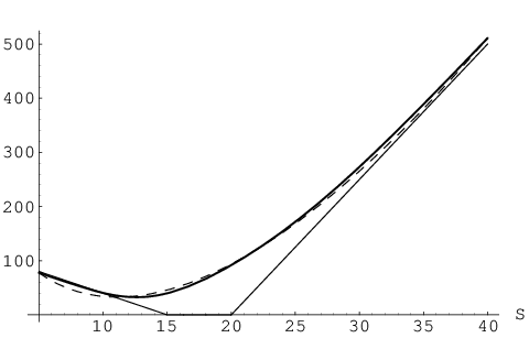
Let us represent the payoff of a strangle as a sum of $K_{P}$ European puts with an exercise price $E_{P}$ and $K_{C}$ European calls with an exercise price $E_{C}$ which have the same expiry date $T$. We can choose in an appropriate way the parameters $m,d_{1},d_{2}$ of the explicit solution (4.46) such that this solution approximates the payoff of a strangle $u_{strangle}(S,T)$,

$$u_{strangle}(S,T)=K_{P}\max{\left(E_{P}-S,0\right)}+K_{C}\max{\left(S-E_{C},0\right)},~~E_{P}<E_{C}.$$

(5.49)

This is shown in Figure 2.

Let us now investigate the asymptotic properties of solutions (4.46) for $S\to 0$ and for $S\to\infty$. The asymptotic behaviour of the function (4.46) for $S\to 0$ can be described as follows,

	$\displaystyle\rho u(S,t)$	$\displaystyle\sim$	$\displaystyle(m^{4})^{1/3}\exp\left(\frac{\sigma^{2}}{8}t\right)+S\ln S$		(5.50)
		$\displaystyle-$	$\displaystyle S\left(\frac{\sigma^{2}t}{8}+\ln((2m)^{4})^{1/3}\right)-S^{3/2}\frac{4\exp{\left(-\frac{\sigma^{2}t}{16}\right)}}{3(m^{2})^{1/3}}+O(S^{5/2}),~~S\to 0.$

The main term in formula (5.50) depends on the time and on the constant $m.$ We can choose $m$ to model payoff properties. From this decomposition it follows immediately that for all solutions from this family the denominator in equation (1.2) vanishes in the point $S=0$. In order to avoid this singularity we exclude the point $S=0$ from the intervals where the numerical investigations are done.

The main term of the asymptotic expansion of $u(S,t)$ for $S\to\infty$,

	$\displaystyle\rho~u(S,t)$	$\displaystyle\sim$	$\displaystyle 3S\ln S-S\left(\frac{3\sigma^{2}t}{8}+4\ln\left(\frac{2^{1/3}m}{3}\right)+2\right)$		(5.51)
		$\displaystyle-$	$\displaystyle S^{-1/2}\left(\frac{2}{3}\right)^{3}\exp{\left(\frac{3\sigma^{2}t}{16}\right)}m^{2}+O(S^{-5/4}),~~S\to\infty,$

is equal to $3S\ln S.$ This term is independent of any integration constant or time. Hence all solutions in this family have the same asymptotic behaviour for $S\to\infty$.

From the financial point of view it is important to study the dependencies of the obtained solutions on different parameters, for instance, on time, on volatility or on the price of the underlying asset, etc. In this way we get information about the sensitivity of our product with respect to a change of one of these parameters. Using the explicit formula for the solutions (4.46) it is easy to represent these dependencies graphically, see Figures 4 - 6. The time dependence of the solutions (4.46) is very weak but still present as we can see on Figure 6.

The obtained family of solutions (4.46) can be used as a benchmark for testing of numerical methods. We suggest the following procedure. We use the solutions (4.46) with boundary conditions which we can obtain just by fixing the time to test numerical methods. These boundary conditions are smooth. Then we take one of the numerical methods and try to reproduce the analytical solution. In this manner we can check on each time step the reached accuracy and adjust the parameters of the grid and the numerical scheme. Thereafter we can be sure that for all smooth boundary conditions of the same type as studied we obtain numerical solutions with nearly the same accuracy.

Now if we apply this method to boundary conditions with worse properties we can be sure that it works at least in the case of an approximation of these boundary conditions by very close but smooth ones. In case of an European call option we have a continuous payoff function $u_{1}(S,T)$,

$$u_{1}(S,T)=\max(S-E,0),$$

(5.52)

where $E$ is the exercise price and $T$ is the expiry date, which is not differentiable in $S=E.$ We can make it smooth by just replacing the payoff $u_{1}(S,T)$ in the neighbourhood of the exercise price $E$. Usually one takes as such smooth function a solution of the linear Black–Scholes formula (5.53) for $t\sim T.$ Then we can compare the results of numerical calculations in both cases. If they do not have any significant difference we can use the same method also in case of continuous boundary conditions and relax the condition of smoothness.

As a first example we take an explicit method for a numerical solution of equation (1.2). This method can be used to find numerically solutions to the linear Black–Scholes model

$$u_{t}+\frac{\sigma^{2}}{2}S^{2}u_{SS}+rSu_{S}-ru=0,$$

(5.53)

where $r$ is the interest rate. It gives proper results for the special relation between $\Delta S^{2}$ and $\Delta t$, where by $\Delta S,\Delta t$ we denote correspondingly the mesh sizes of the discretization of $S$ and $t$ intervals. We applied this method to the nonlinear equation (1.2). We proved that in all studied cases the explicit method diverges independently from the chosen relation between $\Delta S^{2}$ and $\Delta t$. It follows that the explicit method is not reasonable in this nonlinear case.

Another way to solve equation (1.2) numerically is to use the completely implicit method. For the linear Black–Scholes model (5.53) it gives proper results for arbitrary relations between $\Delta S^{2}$ and $\Delta t.$ For a nonlinear equation this method leads to a system of nonlinear algebraic or transcendental equations. An attempt to solve such a system can easily exceed the possibilities of a modern computer due to the very fast with growing grid size. We used this method to reproduce the explicit solutions (4.46) with appropriate accuracy. Thereby we used equidistant grids with $16,28$ and $42$ space nodes and with $15$ and $30$ time levels. We reached the relative accuracy of order of $0.2\%$ .

Then we used this completely implicit method to calculate the value of derivatives governed by equation (1.2) with usual payoff functions.
Let us describe shortly the system of difference equations which we used. It was obtained by replacing the derivatives in the $t$ and $S$ directions in the following way,

	$\displaystyle\frac{\partial u}{\partial t}$	$\displaystyle=$	$\displaystyle\frac{u(S_{i},t_{j+1})-u(S_{i},t_{j})}{\tau}+O(\tau),$
	$\displaystyle\frac{\partial^{2}u}{\partial S^{2}}$	$\displaystyle=$	$\displaystyle\frac{u(S_{i+1},t_{j})-2u(S_{i},t_{j})+u(S_{i-1},t_{j})}{h^{2}}+O(h^{2}),$		(5.54)

where $\tau=\Delta t$ is the time step and $h=\Delta S$ the space step. For each fixed $j$ we obtain a system of $N_{S}-1$ equations

	$\displaystyle\frac{u_{ij+1}}{4}\,\left(\frac{h^{2}}{S_{i}}-\rho(u_{i-1j}-2u_{ij}+u_{i+1j})\right)^{2}-\frac{u_{ij}}{4}\,\left(\frac{h^{2}}{S_{i}}-\rho(u_{i-1j}-2u_{ij}+u_{i+1j})\right)^{2}$
	$\displaystyle~~~~~~+\frac{\tau\sigma^{2}h^{2}}{8}\,(u_{i-1j}-2u_{ij}+u_{i+1j})=0,\qquad i=\overline{2,N_{S}},\,\,j=\overline{N_{t},1},$		(5.55)

for the internal points, where $N_{t}$ is the number of time layers and $N_{S}+1$ is the number of grid nodes in space direction. In this case we used the final conditions, i.e., the knowledge of the values $u(S,T)$ and calculated the values for $u(S,t)$ backwards to $t=0$. In the system (5) the values on the layer $j+1$ are known and the values on the layer $j$ are unknown functions. On the boundaries $S_{1}$ and $S_{N_{S}+1}$ the values $u_{ij}$ are defined for each fixed $j$ by the function $u_{bound}(S,t)$ in accordance with the used boundary conditions. The complete system of difference equations has the form

References

- [1] D. Duffie, W. Fleming, H. Soner et al. Hedging in incomplete markers with HARA utility. J. Econ. Dyn. Control, 21 (1997) 753–782.
- [2] J. Fouque, G. Papanicolaou, R. Sircar et al. Singular perturbations in option pricing. SIAM J. Appl. Math., 63 (2003) 1648–1665.
- [3] R. Frey. Perfect Option Replication for a Large Trader. Ph.D. thesis, ETH Zurich (1996).
- [4] R. Frey. Market illiquidity as a source of model risk in dynamic hedging. Model Risk, (2000) 125–136.
- [5] R. Frey. Risk minimization with incomplete information in a model for high-frequency data. Mathematical Finance, 10 (2000) 215–225.
- [6] R. Frey and P. Patie. Risk management for derivatives with market illiquidities. Technical report, RiskLab, Department of Mathematics, ETH Zurich (2002).
- [7] R. Frey and A. Stremme. Market volatility and feedback effect from dynamic hedging. Mathematical Finance, 7 (1997) 351–374.
- [8] G. Gaeta. Nonlinear Symmetries and Nonlinear Equations, volume 299 of Mathematics and its Applications. Kluwer Academic Publishers, Dordrecht, NL Boston, USA London UK (1994).
- [9] N. H. Ibragimov. Elementary Lie Group Analysis and Ordinary Differential Equations. John Wiley&Sons, Chischester, USA New York, USA Weinheim, Germany Brisbane, USA Singapore, Singapore Toronto Canada etc. (1999).
- [10] S. Lie. Vorlesungen über Differentialgleichungen mit bekannten infinitesimalen Transformationen. Teubner, Leipzig, Germany (1912).
- [11] P. J. Olver. Application of Lie groups to differential equations. Springer-Verlag, New York, USA (1986).
- [12] L. V. Ovsiannikov. Group Analysis of Differential Equations. Academic Press, New York, USA (1982).
- [13] P. Schonbucher and P. Wilmott. Hedging in illiquid markets: Nonlinear effects. Z. Angew. Math. Mech., 76 (1996) 81–84.
- [14] P. Schonbucher and P. Wilmott. The feedback effect of hedging in illiquid markets. SIAM J. Appl. Math., 61 (2000) 232–272.
- [15] K. Sircar and G. Papanicolaou. General Black-Scholes models accounting for increased market volatility from hedging strategies. Appl. Math. Finance, 5 (1998) 45–82.
- [16] H. Stephani. Differential Gleichungen: Symmetrien und Lösungsmethoden. Spektrum Akademischer Verlag GmbH, Heidelberg, Germany (1994).
- [17] A. Whalley and P. Wilmott. An asymptotic analysis of an optimal hedging model for option pricing with transaction costs. Mathematical Finance, 7 (1997) 307–324.
- [18] A. Whalley and P. Wilmott. Optimal hedging of options with small but arbitrary transaction cost structure. Eur. J. Appl. Math., 10 (1999) 117–139.
- [19] P. Wilmott and A. Whalley. Option pricing, transaction costs and nonlinearities. Z. Angew. Math. Mech., 76 (1996) 85–88.
The Greeks for solutions (4.46).
The sensitivity parameters and Vega for solutions (4.46).