跳到论文正文
W Papers独立论文阅读器 arXiv:math/0604094 论文正文 计算阅读时间 · 0%
引用这篇论文根据当前论文元数据生成,正式投稿前建议核对。


License: Assumed arXiv.org perpetual non-exclusive license
arXiv:math/0604094v1 [math.QA] 05 Apr 2006

Generalized Volume Conjecture and the A-Polynomials:
The Neumann–Zagier Potential Function as a Classical Limit of Quantum Invariant

Kazuhiro Hikami Email address: hikami@phys.s.u-tokyo.ac.jp URL: http://gogh.phys.s.u-tokyo.ac.jp/~hikami/ Address: Department of Physics, Graduate School of Science,
University of Tokyo,
Hongo 7–3–1, Bunkyo, Tokyo 113–0033, Japan.
Date: April 4, 2006
Abstract.

We study quantum invariant Zγ​(ℳ)Z_{\gamma}(\mathcal{M}) for cusped hyperbolic 3-manifold ℳ\mathcal{M}. We construct this invariant based on oriented ideal triangulation of ℳ\mathcal{M} by assigning to each tetrahedron the quantum dilogarithm function, which is introduced by Faddeev in studies of the modular double of the quantum group. Following Thurston and Neumann–Zagier, we deform a complete hyperbolic structure of ℳ\mathcal{M}, and correspondingly we define quantum invariant Zγ​(ℳu)Z_{\gamma}(\mathcal{M}_{u}). This quantum invariant is shown to give the Neumann–Zagier potential function in the classical limit γ→0\gamma\to 0, and the A-polynomial can be derived from the potential function. We explain our construction by taking examples of 3-manifolds such as complements of hyperbolic knots and punctured torus bundle over the circle.

1. Introduction

Since the quantum invariant of knots/links and 3-manifolds as a generalization of the Jones polynomial [25] is constructed by Witten [53] by use of the Chern–Simons path integral, studies on quantum invariants have been much developed. Recently geometrical interpretations of the quantum invariants have received interests since Kashaev observed an intriguing relationship [29] between the hyperbolic volume and his knot invariant, which is later identified with a specific value of the NN-colored Jones polynomial J𝒦​(N,e2​π​i/N)J_{\mathcal{K}}\left(N;\mathrm{e}^{2\pi\mathrm{i}/N}\right) [41] (here the NN-colored Jones polynomial is normalized to be Junknot​(N,q)=1J_{\text{unknot}}(N;q)=1). Namely the hyperbolic volume of the knot complement S3∖𝒦S^{3}\setminus\mathcal{K} is conjectured to dominate the asymptotics of the invariant J𝒦​(N,e2​π​i/N)J_{\mathcal{K}}\left(N;\mathrm{e}^{2\pi\mathrm{i}/N}\right) in the large-NN limit N→∞N\to\infty,

limN→∞2​πN​log⁡|J𝒦​(N,e2​π​i/N)|=Vol⁡(S3∖𝒦)\lim_{N\to\infty}\frac{2\,\pi}{N}\log\left|J_{\mathcal{K}}\left(N;\mathrm{e}^{2\pi\mathrm{i}/N}\right)\right|=\Vol(S^{3}\setminus\mathcal{K}) (1.1)

This “volume conjecture” is generalized for other values (near the NN-th root of unity) of the NN-colored Jones polynomial [18] (see also Refs. [39, 40]), and a relationship with the A-polynomial is conjectured; when we define bb by

b=−dd​alimN,k→∞N/k=a1klogJ𝒦(N;e2​π​i/k)b=-\frac{\mathrm{d}}{\mathrm{d}a}\,\lim_{\begin{subarray}{c}N,k\to\infty\\ N/k=a\end{subarray}}\frac{1}{k}\,\log J_{\mathcal{K}}\left(N;\mathrm{e}^{2\pi\mathrm{i}/k}\right) (1.2)

the pair (eb,−ei​a)\left(\mathrm{e}^{b},-\mathrm{e}^{\mathrm{i}a}\right) is a zero locus of the A-polynomial for knot 𝒦\mathcal{K}. This is checked numerically for twist knots [22].

The A-polynomial is defined as an algebraic curve of eigenvalues of the S​L​(2,ℂ)SL(2;\mathbb{C}) representation of the boundary torus of knot 𝒦\mathcal{K} [9] (see also Ref. [10]). This can be computed from triangulation of the knot complement ℳ=S3∖𝒦\mathcal{M}=S^{3}\setminus\mathcal{K} into ideal tetrahedra in the hyperbolic space ℍ3\mathbb{H}^{3} once the fundamental group has a irreducible representation ρ\rho into P​S​L​(2,ℂ)PSL(2;\mathbb{C}) which is identified with the orientation-preserving isometries of ℍ3\mathbb{H}^{3};

ρ:π1​(ℳ)→P​S​L​(2,ℂ)≃Isom+⁡(ℍ3)\rho:\pi_{1}(\mathcal{M})\to PSL(2;\mathbb{C})\simeq\Isom^{+}(\mathbb{H}^{3})

Up to conjugation, the meridian μ\mu and the longitude of the boundary torus of 𝒦\mathcal{K} have

ρ⁡(μ)=(m∗01/m)\displaystyle\rho(\mu)=\begin{pmatrix}m&*\\ 0&1/m\end{pmatrix}
ρ⁡(λ)=(ℓ∗01/ℓ)\displaystyle\rho(\lambda)=\begin{pmatrix}\ell&*\\ 0&1/\ell\end{pmatrix}

Another geometrical aspect of the NN-colored Jones polynomial J𝒦​(N,q)J_{\mathcal{K}}(N;q) as a relationship with the A-polynomial is proposed as “AJ conjecture” [17]; recursion relation of the colored Jones polynomial with respect to NN is conjectured to be related to the A-polynomial A𝒦​(ℓ,m)A_{\mathcal{K}}(\ell,m). This conjecture is proved for the torus knots [23] and the 2-bridge knots [35].

In this paper, we introduce quantum invariant for cusped hyperbolic manifold ℳ\mathcal{M} and its deformation ℳu\mathcal{M}_{u} à la Thurston [50] following Refs. [19, 20, 21], and study a classical limit thereof. Based on a triangulation of cusped 3-manifold ℳ\mathcal{M}, we define quantum invariant Zγ​(ℳu)Z_{\gamma}(\mathcal{M}_{u}) by assigning Faddeev’s quantum dilogarithm function to each oriented ideal tetrahedron. Originally Kashaev introduced his invariant J𝒦​(N,e2​π​i/N)J_{\mathcal{K}}\left(N;\mathrm{e}^{2\pi\mathrm{i}/N}\right) for triangulated 3-manifolds, although the RR-matrix construction is developed subsequently [28]. He studied Faddeev’s quantum dilogarithm function when qq is a root of unity [13, 26] (see also Ref. [2]), and assigning the quantum dilogarithm function to ideal tetrahedron he defined invariant [28, 27]. In this sense, our invariant Zγ​(ℳ)Z_{\gamma}(\mathcal{M}) for ℳ\mathcal{M} with complete hyperbolic structure can be regarded as a non-compact Uq​(s​l​(2,ℝ))U_{q}(sl(2;\mathbb{R})) analogue of the Kashaev invariant, and an asymptotic behavior of Zγ​(S3∖𝒦)Z_{\gamma}(S^{3}\setminus\mathcal{K}) in the limit γ→0\gamma\to 0 should coincide with that of the Kashaev invariant J𝒦​(N,e2​π​i/N)J_{\mathcal{K}}\left(N;\mathrm{e}^{2\pi\mathrm{i}/N}\right) in the limit N→∞N\to\infty.

This paper is organized as follows. In Section 2 we recall definitions of quantum dilogarithm function, and we discuss properties of this function. In Section 3, we shall reveal that the three-dimensional hyperbolic geometry naturally arises from the quantum dilogarithm function in the classical limit γ→0\gamma\to 0 as was clarified in Ref. [19]. Then we define the quantum invariant Zγ​(ℳu)Z_{\gamma}(\mathcal{M}_{u}) for a deformation of complete hyperbolic cusped 3-manifold ℳ\mathcal{M}. Based on a triangulation of ℳ\mathcal{M}, we construct the invariant by assigning quantum dilogarithm function to oriented ideal tetrahedron. We discuss that the Neumann–Zagier potential function appears in a classical limit of Zγ​(ℳ)Z_{\gamma}(\mathcal{M}). In Section 4, we take several examples of cusped hyperbolic manifolds such as complements of hyperbolic knots and punctured torus bundle over the circle, and explain our assertion in detail. We shall also give a list for other manifolds in Appendix. The last section is devoted to conclusions and discussions.

2. Quantum Dilogarithm Function

We define a function Φγ​(φ)\Phi_{\gamma}(\varphi) by an integral form following Ref. [12]. We set γ∈ℝ\gamma\in\mathbb{R}, and for |Im⁡φ|<π|\operatorname{Im}\varphi|<\pi, we define

Φγ​(φ)=exp⁡(∫ℝ+i​ 0e−i​φ​x4​sinh⁡(γ​x)​sinh⁡(π​x)​d​xx)\Phi_{\gamma}(\varphi)=\exp\left(\int\limits_{\mathbb{R}+\mathrm{i}\,0}\frac{\mathrm{e}^{-\mathrm{i}\,\varphi\,x}}{4\sinh(\gamma\,x)\,\sinh(\pi\,x)}\,\frac{\mathrm{d}x}{x}\right) (2.1)

The Faddeev integral (2.1), which we call the quantum dilogarithm function, is also related to the double sine function [31, 48, 34], the hyperbolic gamma function [46, 1] and the quantum exponential function [54]. We see that the integral Φγ​(φ)\Phi_{\gamma}(\varphi) has a duality,

Φπ2γ​(φ)=Φγ​(γπ​φ)\Phi_{\frac{\pi^{2}}{\gamma}}(\varphi)=\Phi_{\gamma}\left(\frac{\gamma}{\pi}\,\varphi\right) (2.2)

and that it satisfies the inversion relation,

Φγ​(φ)⋅Φγ​(−φ)=exp⁡(−12​i​γ​(φ22+π2+γ26))\Phi_{\gamma}(\varphi)\cdot\Phi_{\gamma}(-\varphi)=\exp\left(-\frac{1}{2\,\mathrm{i}\,\gamma}\Bigl(\frac{\varphi^{2}}{2}+\frac{\pi^{2}+\gamma^{2}}{6}\Bigr)\right) (2.3)

The Faddeev integral satisfies the difference equations;

Φγ​(φ+i​γ)Φγ​(φ−i​γ)\displaystyle\frac{\Phi_{\gamma}(\varphi+\mathrm{i}\,\gamma)}{\Phi_{\gamma}(\varphi-\mathrm{i}\,\gamma)} =11+eφ\displaystyle=\frac{1}{1+\mathrm{e}^{\varphi}} (2.4a)
Φγ​(φ+i​π)Φγ​(φ−i​π)\displaystyle\frac{\Phi_{\gamma}(\varphi+\mathrm{i}\,\pi)}{\Phi_{\gamma}(\varphi-\mathrm{i}\,\pi)} =11+eπγ​φ\displaystyle=\frac{1}{1+\mathrm{e}^{\frac{\pi}{\gamma}\varphi}} (2.4b)

Due to these relations, the integral Φγ​(φ)\Phi_{\gamma}(\varphi) defined in (2.1) is analytically continued to φ∈ℂ\varphi\in\mathbb{C}, and we see that

zeros of (Φγ​(φ))±1={φ=∓i((2m+1)γ+(2n+1)π)|m,n∈ℤ≥0}\text{zeros of $\bigl(\Phi_{\gamma}(\varphi)\bigr)^{\pm 1}$}=\Bigl\{\varphi=\mp\mathrm{i}\,\bigl((2\,m+1)\,\gamma+(2\,n+1)\,\pi\bigr)\ \big|\ m,n\in\mathbb{Z}_{\geq 0}\Bigr\} (2.5)

The most important properties of the Faddeev integral is that it fulfills the pentagon identity [13, 12]

Φγ​(p^)​Φγ​(q^)=Φγ​(q^)​Φγ​(p^+q^)​Φγ​(p^)\Phi_{\gamma}(\hat{p})\,\Phi_{\gamma}(\hat{q})=\Phi_{\gamma}(\hat{q})\,\Phi_{\gamma}(\hat{p}+\hat{q})\,\Phi_{\gamma}(\hat{p}) (2.6)

where p^\hat{p} and q^\hat{q} are the canonically conjugate operators satisfying the Heisenberg commutation relation,

[p^,q^]=p^​q^−q^​p^=−2​i​γ[\hat{p}~,~\hat{q}]=\hat{p}\,\hat{q}-\hat{q}\,\hat{p}=-2\,\mathrm{i}\,\gamma (2.7)

By this commuting relation, we call a limit γ→0\gamma\to 0 a classical limit.

We use 𝐕\mathbf{V} as the momentum space |p⟩|p\rangle with p∈ℝp\in\mathbb{R} which is an eigenstate of the momentum operator;

p^​|p⟩=p​|p⟩.\hat{p}\,|p\rangle=p\,|p\rangle. (2.8)

A reason of the quantum dilogarithm function reveals when we take a classical limit γ→0\gamma\to 0. In this limit, the Faddeev integral reduces to

Φγ​(φ)∼exp⁡(12​i​γ​Li_2⁡(−eφ))\Phi_{\gamma}(\varphi)\sim\exp\left(\frac{1}{2\,\mathrm{i}\,\gamma}\,\Li(-\mathrm{e}^{\varphi})\right) (2.9)

where Li_2⁡(x)\Li(x) denotes the Euler dilogarithm function defined by (see, e.g., Refs. [36, 32])

Li_2⁡(x)=∑n=1∞xnn2\Li(x)=\sum_{n=1}^{\infty}\frac{x^{n}}{n^{2}} (2.10)

where |x|≤1|x|\leq 1. For x∈ℂx\in\mathbb{C}, we use the integral form

Li_2(x)=−∫0xlog(1−s)d​ss\Li(x)=-\int_{0}^{x}\log(1-s)\,\frac{\mathrm{d}s}{s}

where the branch of log⁡(1−s)\log(1-s) is on ℂ∖[1,∞)\mathbb{C}\setminus[1,\infty) for which log⁡(1−0)=0\log(1-0)=0. See that the inversion relation (2.3) of the quantum dilogarithm function Φγ​(φ)\Phi_{\gamma}(\varphi) gives that of the Euler dilogarithm function as

Li_2⁡(−ex)+Li_2⁡(−e−x)+x22+π26=0\Li(-\mathrm{e}^{x})+\Li(-\mathrm{e}^{-x})+\frac{x^{2}}{2}+\frac{\pi^{2}}{6}=0

We note that the Fourier transformation of the Faddeev integral can be computed as follows [54, 14, 5, 31];

14​π​γ​∫ℝd​y​Φγ​(y)​e12​i​γ​x​y=Φγ​(−x+i​π+i​γ)​e12​i​γ​(x22−12​π​γ−π2+γ26)\displaystyle\frac{1}{\sqrt{4\,\pi\,\gamma}}\int\limits_{\mathbb{R}}\mathrm{d}y\ \Phi_{\gamma}(y)\,\mathrm{e}^{\frac{1}{2\,\mathrm{i}\,\gamma}\,x\,y}=\Phi_{\gamma}(-x+\mathrm{i}\pi+\mathrm{i}\gamma)\,\mathrm{e}^{\frac{1}{2\,\mathrm{i}\,\gamma}\left(\frac{x^{2}}{2}-\frac{1}{2}\pi\gamma-\frac{\pi^{2}+\gamma^{2}}{6}\right)} (2.11)
14​π​γ​∫ℝd​y​1Φγ​(y)​e12​i​γ​x​y=1Φγ​(x−i​π−i​γ)​e−12​i​γ​(x22−12​π​γ−π2+γ26)\displaystyle\frac{1}{\sqrt{4\,\pi\,\gamma}}\int\limits_{\mathbb{R}}\mathrm{d}y\ \frac{1}{\Phi_{\gamma}(y)}\,\mathrm{e}^{\frac{1}{2\,\mathrm{i}\,\gamma}x\,y}=\frac{1}{\Phi_{\gamma}(x-\mathrm{i}\,\pi-\mathrm{i}\,\gamma)}\,\mathrm{e}^{-\frac{1}{2\,\mathrm{i}\,\gamma}\left(\frac{x^{2}}{2}-\frac{1}{2}\pi\gamma-\frac{\pi^{2}+\gamma^{2}}{6}\right)} (2.12)

To see a relationship between the integral Φγ​(φ)\Phi_{\gamma}(\varphi) with geometry, we define the SS-operator acting on 𝐕⊗𝐕\mathbf{V}\otimes\mathbf{V} by

S1,2=e12​i​γ​q^1​p^2​Φγ​(p^1+q^2−p^2)S_{1,2}=\mathrm{e}^{\frac{1}{2\,\mathrm{i}\,\gamma}\,\hat{q}_{1}\,\hat{p}_{2}}\,\Phi_{\gamma}(\hat{p}_{1}+\hat{q}_{2}-\hat{p}_{2}) (2.13)

Here the Heisenberg operators p^j\hat{p}_{j} and q^j\hat{q}_{j} act on the jj-th vector space of 𝐕⊗𝐕\mathbf{V}\otimes\mathbf{V}, i.e. p^1=p^⊗1\hat{p}_{1}=\hat{p}\otimes 1, p^2=1⊗p^\hat{p}_{2}=1\otimes\hat{p}, and so on. Then the pentagon identity (2.6) can be rewritten in a compact form;

S2,3​S1,2=S1,2​S1,3​S2,3S_{2,3}\,S_{1,2}=S_{1,2}\,S_{1,3}\,S_{2,3} (2.14)

where Sj,kS_{j,k} acts on the jj- and kk-th spaces of 𝐕⊗𝐕⊗𝐕\mathbf{V}\otimes\mathbf{V}\otimes\mathbf{V}. Matrix elements can be computed by use of (2.11) and (2.12);

⟨p1,p2​|S1,2|​p1′,p2′⟩=14​π​γ​δ​(p1+p2−p1′)⋅Φγ​(p2′−p2+i​π+i​γ)​e12​i​γ​(−π2+γ26−γ​π2+p1​(p2′−p2))\displaystyle\begin{split}&\langle p_{1},p_{2}\ |\ S_{1,2}\ |\ p_{1}^{\prime},p_{2}^{\prime}\rangle\\ &\qquad=\frac{1}{\sqrt{4\,\pi\,\gamma}}\,\delta(p_{1}+p_{2}-p_{1}^{\prime})\cdot\Phi_{\gamma}(p_{2}^{\prime}-p_{2}+\mathrm{i}\,\pi+\mathrm{i}\,\gamma)\,\mathrm{e}^{\frac{1}{2\,\mathrm{i}\,\gamma}\left(-\frac{\pi^{2}+\gamma^{2}}{6}-\frac{\gamma\,\pi}{2}+p_{1}\,(p_{2}^{\prime}-p_{2})\right)}\end{split} (2.15a)
⟨p1,p2​|S1,2−1|​p1′,p2′⟩=14​π​γ​δ​(p1−p1′−p2′)​1Φγ​(p2−p2′−i​π−i​γ)​e12​i​γ​(π2+γ26+γ​π2−p1′​(p2−p2′))\displaystyle\begin{split}&\langle p_{1},p_{2}\ |\ S_{1,2}^{~-1}\ |\ p_{1}^{\prime},p_{2}^{\prime}\rangle\\ &\qquad=\frac{1}{\sqrt{4\,\pi\,\gamma}}\,\delta(p_{1}-p_{1}^{\prime}-p_{2}^{\prime})\,\frac{1}{\Phi_{\gamma}(p_{2}-p_{2}^{\prime}-\mathrm{i}\,\pi-\mathrm{i}\,\gamma)}\,\mathrm{e}^{\frac{1}{2\mathrm{i}\gamma}\left(\frac{\pi^{2}+\gamma^{2}}{6}+\frac{\gamma\,\pi}{2}-p_{1}^{\prime}(p_{2}-p_{2}^{\prime})\right)}\end{split} (2.15b)

In the classical limit γ→0\gamma\to 0, we find by use of (2.9) that the SS-operators (2.15) reduce to

⟨p1,p2​|S1,2|​p1′,p2′⟩\displaystyle\langle p_{1},p_{2}\ |\ S_{1,2}\ |\ p_{1}^{\prime},p_{2}^{\prime}\rangle ∼δ⁡(p1+p2−p1′)⋅exp⁡(−12​i​γ​V​(p2′−p2,p1))\displaystyle\sim\delta(p_{1}+p_{2}-p_{1}^{\prime})\cdot\exp\left(-\frac{1}{2\,\mathrm{i}\,\gamma}\,V(p_{2}^{\prime}-p_{2},p_{1})\right) (2.16a)
⟨p1,p2​|S1,2−1|​p1′,p2′⟩\displaystyle\langle p_{1},p_{2}\ |\ S_{1,2}^{-1}\ |\ p_{1}^{\prime},p_{2}^{\prime}\rangle ∼δ⁡(p1−p1′−p2′)⋅exp⁡(12​i​γ​V​(p2−p2′,p1′))\displaystyle\sim\delta(p_{1}-p_{1}^{\prime}-p_{2}^{\prime})\cdot\exp\left(\frac{1}{2\,\mathrm{i}\,\gamma}\,V(p_{2}-p_{2}^{\prime},p_{1}^{\prime})\right) (2.16b)

where we have defined the function V⁡(x,y)V(x,y) by

V⁡(x,y)=π26−Li_2⁡(ex)−x​y.V(x,y)=\frac{\pi^{2}}{6}-\Li(\mathrm{e}^{x})-x\,y. (2.17)

We see that the function V⁡(x,y)V(x,y) satisfies partial differential equations;

V⁡(x,y)=L⁡(1−ex)+12​(x​∂V⁡(x,y)∂x+y​∂V⁡(x,y)∂y)\displaystyle V(x,y)=L(1-\mathrm{e}^{x})+\frac{1}{2}\left(x\,\frac{\partial V(x,y)}{\partial x}+y\,\frac{\partial V(x,y)}{\partial y}\right) (2.18)
Im⁡V⁡(x,y)=D⁡(1−ex)+log⁡|ex|⋅Im⁡(∂∂x​V​(x,y))+log⁡|ey|⋅Im⁡(∂∂y​V​(x,y))\displaystyle\operatorname{Im}\,V(x,y)=D(1-\mathrm{e}^{x})+\log|\mathrm{e}^{x}|\cdot\operatorname{Im}\,\biggl(\frac{\partial}{\partial x}V(x,y)\biggr)+\log|\mathrm{e}^{y}|\cdot\operatorname{Im}\,\biggl(\frac{\partial}{\partial y}V(x,y)\biggr) (2.19)

Here the Rogers dilogarithm L⁡(z)L(z) and the Bloch–Wigner function D⁡(z)D(z) are respectively defined in terms of the Euler dilogarithm function (2.10) by

L⁡(z)\displaystyle L(z) =Li_2⁡(z)+12​log⁡z​log⁡(1−z)\displaystyle=\Li(z)+\frac{1}{2}\log z\,\log(1-z) (2.20)
D⁡(z)\displaystyle D(z) =Im⁡Li_2⁡(z)+arg⁡(1−z)⋅log⁡|z|\displaystyle=\operatorname{Im}\,\Li(z)+\arg(1-z)\cdot\log|z| (2.21)

both of which fulfill the pentagon identity (see, e.g., Ref. [36]);

L⁡(z)−L⁡(w)+L⁡(wz)−L⁡(1−z−11−w−1)+L⁡(1−z1−w)=π26\displaystyle L(z)-L(w)+L\left(\frac{w}{z}\right)-L\left(\frac{1-z^{-1}}{1-w^{-1}}\right)+L\left(\frac{1-z}{1-w}\right)=\frac{\pi^{2}}{6} (2.22)
D⁡(z)−D⁡(w)+D⁡(wz)−D⁡(1−z−11−w−1)+D⁡(1−z1−w)=0\displaystyle D(z)-D(w)+D\left(\frac{w}{z}\right)-D\left(\frac{1-z^{-1}}{1-w^{-1}}\right)+D\left(\frac{1-z}{1-w}\right)=0 (2.23)

3. Quantum Invariant and Potential Function

The result that the SS-operator satisfies the pentagon identity (2.14) indicates that we can assign (oriented) tetrahedron to each SS-operator. See Refs. [7, 30] (also Ref. [8]) for another interpretation as a quantization of the Teichmüller theory. In the classical limit γ→0\gamma\to 0, imaginary part of the SS-operator gives the Bloch–Wigner function D⁡(z)D(z) which denotes the hyperbolic volume of the ideal tetrahedron Δ⁡(z)\Delta(z) with totally geodesic faces which has a modulus zz (see, e.g., Refs. [3, 38, 50]). Extra terms in (2.19) including partial differentials of V⁡(x,y)V(x,y) can be neglected when we assume a saddle point condition as will be discussed later, and we can assign the oriented hyperbolic ideal tetrahedra to these SS-operators as follows [19];

⟨a,b|S|c,d⟩\displaystyle\left\langle a,b\ \middle|\ S\ \middle|\ c,d\right\rangle =  [Uncaptioned image]  =  [Uncaptioned image] \displaystyle=\mbox{ \raisebox{-45.52458pt}{ \includegraphics[scale]{tetrahedronProj.1.eps} } }=\mbox{ \raisebox{-45.52458pt}{ \includegraphics[scale]{tetrahedron.1.eps} } } (3.1)
⟨a,b|S−1|c,d⟩\displaystyle\left\langle a,b\ \middle|\ S^{-1}\ \middle|\ c,d\right\rangle =  [Uncaptioned image]  =  [Uncaptioned image] \displaystyle=\mbox{ \raisebox{-45.52458pt}{ \includegraphics[scale]{tetrahedronDualProj.1.eps} } }=\mbox{ \raisebox{-45.52458pt}{ \includegraphics[scale]{tetrahedronDual.1.eps} } } (3.2)

Namely in the momentum space representation we assign four momentum parameters {a,b,c,d}\{a,b,c,d\} to faces of tetrahedron. This differs from the (quantum) 6​j6j symbol as a solution of the pentagon identity [45, 33], which was used to define the topological (quantum) gravity.

Here both ideal tetrahedra have the modulus z=ed−bz=\mathrm{e}^{d-b}, and we mean that the dihedral angles are given by

z⁡[1]\displaystyle z[1] =z=ed−b\displaystyle=z=\mathrm{e}^{d-b}
z⁡[2]\displaystyle z[2] =1−1z\displaystyle=1-\frac{1}{z}
z⁡[3]\displaystyle z[3] =11−z\displaystyle=\frac{1}{1-z}

The cross sections by the horosphere is similar to the triangle in ℂ\mathbb{C} with vertices 00, 11, and zz (see Fig. 1), and we have z⁡[1]​z​[2]​z​[3]=−1z[1]\,z[2]\,z[3]=-1. See that the opposite edges of tetrahedra have the same dihedral angles. Then the hyperbolic volume of the ideal tetrahedron Δ⁡(z)\Delta(z) with modulus zz is given by [50]

Vol⁡(Δ⁡(z))\displaystyle\Vol\left(\Delta(z)\right) =D⁡(z)\displaystyle=D(z)
=L​(arg⁡(z⁡[1]))+L​(arg⁡(z⁡[2]))+L​(arg⁡(z⁡[3]))\displaystyle=\text{\cyr L}\left(\arg(z[1])\right)+\text{\cyr L}\left(\arg(z[2])\right)+\text{\cyr L}\left(\arg(z[3])\right) (3.3)

where L​(θ)\text{\cyr L}(\theta) is the Lobachevsky function defined by

L​(θ)=12​∑n=1∞sin⁡(2​n​θ)n2\text{\cyr L}(\theta)=\frac{1}{2}\sum_{n=1}^{\infty}\frac{\sin(2\,n\,\theta)}{n^{2}} (3.4)
Refer to caption
Figure 1. Triangle with vertices 00, 11, and zz in ℂ\mathbb{C}. Here we set z⁡[1]=zz[1]=z, z⁡[2]=1−1zz[2]=1-\frac{1}{z}, and z⁡[3]=11−zz[3]=\frac{1}{1-z}.

Any hyperbolic cusped 33-manifold ℳ\mathcal{M} (for simplicity we assume that the manifold ℳ\mathcal{M} has one cusp in this paper) can be ideally triangulated, and it is constructed from finite number of the oriented ideal tetrahedra in (3.1) and (3.2). Other types of oriented ideal tetrahedra, such as one that has a face with loop, are prohibited. So our triangulation sometimes differ from the canonical triangulation used in computer programs, such as SnapPea [52], Knotscape [24], and Snap [11].

To construct 3-manifolds from these ideal tetrahedra, we glue each face to match orientations of edges. Every faces have no loops, so there is no ambiguity in gluing faces together once two faces to be glued are fixed. Furthermore, one finds that in-state |p⟩|p\rangle can glue only with out-states ⟨p|\langle p|, and that we cannot glue two in-states or out-states together. As suggested by the momentum representation of the pentagon identity, gluing two faces, which have same label pp, can be formulated by an integration with respect to pp, ∫ℝd​p​|p⟩​⟨p|\int\limits_{\mathbb{R}}\mathrm{d}p\,|p\rangle\,\langle p|.

By these identifications of the SS-operators as the oriented ideal tetrahedra, the pentagon identity (2.14) is identified with the Pachner move as is depicted in Fig. 2; oriented polytope with 5 vertices can be decomposed into 2 tetrahedra with a face in common, or into 3 tetrahedra with an edge in common. In case of decomposing into 3 tetrahedra, we need a hyperbolic consistency condition around the common edge. This condition coincides with a saddle point condition of the right hand side of (2.14) after substituting (2.15) and taking a classical limit γ→0\gamma\to 0. One can see a coincidence for any other type of gluings such as other choices of orientations in the Pachner move between the hyperbolic consistency condition and the saddle point equations [19].

Refer to caption
Figure 2. Pentagon identity (2.14) is interpreted as the Pachner move.

Once triangulation is given and we know how to glue faces together, we can naturally define the quantum invariant for hyperbolic cusped 33-manifold ℳ\mathcal{M} based on the SS-operator by

Zγ(ℳ)=∫ℝd𝒑δC(𝒑)δG(𝒑)∏i=1M⟨p2​i−1(−),p2​i(−)|Sεi|p2​i−1(+),p2​i(+)⟩Z_{\gamma}(\mathcal{M})=\int\limits_{\mathbb{R}}\mathrm{d}\boldsymbol{p}\,\delta_{C}(\boldsymbol{p})\,\delta_{G}(\boldsymbol{p})\,\prod_{i=1}^{M}\left\langle p_{2i-1}^{(-)},p_{2i}^{(-)}~\middle|~S^{\varepsilon_{i}}~\middle|~p_{2i-1}^{(+)},p_{2i}^{(+)}\right\rangle (3.5)

where 𝒑\boldsymbol{p} denotes a set of variables (p1(±),p2(±),…,p2​M(±))(p_{1}^{(\pm)},p_{2}^{(\pm)},\dots,p_{2M}^{(\pm)}), and εi=±1\varepsilon_{i}=\pm 1 depending on an orientation of tetrahedron. We set MM as the number of ideal tetrahedra. The condition δG​(𝒑)\delta_{G}(\boldsymbol{p}) determines how to glue faces together (“G” stands for “gluing”). Every faces with same momentum mean to be glued together, and the fact that in-states can be glued only with out-states indicates that the gluing condition δG​(𝒑)\delta_{G}(\boldsymbol{p}) is a product of δ⁡(pj(−)−pk(+))\delta\left(p_{j}^{(-)}-p_{k}^{(+)}\right)

We need another geometrical condition δC​(𝒑)\delta_{C}(\boldsymbol{p}) to define invariant besides a way how to glue faces (“C” stands for “completeness”) [21]. We can draw a developing map from an ideal triangulation of 3-manifold, and we need to read off a hyperbolic complete condition. This condition can be written as a constraint for 𝒑\boldsymbol{p} by identifications (3.1) and (3.2). By construction, the partition function Zγ​(ℳ)Z_{\gamma}(\mathcal{M}) is invariant under the Pachner move (Fig. 2), and it is essentially the invariant constructed in Ref. [19].

As was studied by Thurston [51], deformation of the hyperbolic structure on the manifold ℳ\mathcal{M} can be holomorphically parametrized by a parameter uu in a neighborhood of completeness condition u=0u=0. The parameter uu is the logarithm of the eigenvalue of the meridian by the holonomy representation, and we set

m=eum=e^{u} (3.6)

Correspondingly we call such manifold ℳu\mathcal{M}_{u} which is no more complete, and define the invariant by

Zγ(ℳu)=∫ℝd𝒑δC(𝒑;u)δG(𝒑)∏i=1M⟨p2​i−1(−),p2​i(−)|Sεi|p2​i−1(+),p2​i(+)⟩Z_{\gamma}(\mathcal{M}_{u})=\int\limits_{\mathbb{R}}\mathrm{d}\boldsymbol{p}\,\delta_{C}(\boldsymbol{p};u)\,\delta_{G}(\boldsymbol{p})\,\prod_{i=1}^{M}\left\langle p_{2i-1}^{(-)},p_{2i}^{(-)}~\middle|~S^{\varepsilon_{i}}~\middle|~p_{2i-1}^{(+)},p_{2i}^{(+)}\right\rangle (3.7)

Here the condition δC​(𝒑,u)\delta_{C}(\boldsymbol{p};u) follows from that the meridian has a holonomy (3.6). The invariant (3.5) for ℳ\mathcal{M} with complete hyperbolic structure follows from (3.7) by assuming a completeness u=0u=0 of the hyperbolic structure of ℳu\mathcal{M}_{u};

Zγ​(ℳ)=Zγ​(ℳu=0)Z_{\gamma}(\mathcal{M})=Z_{\gamma}\left(\mathcal{M}_{u=0}\right) (3.8)

because

δC​(𝒑)=δC​(𝒑,u=0)\delta_{C}(\boldsymbol{p})=\delta_{C}(\boldsymbol{p};u=0) (3.9)

We now study a classical limit of our quantum invariant Zγ​(ℳu)Z_{\gamma}(\mathcal{M}_{u}). When we take a limit γ→0\gamma\to 0 by use of (2.16), the quantum invariant defined by (3.7) becomes

Zγ​(ℳu)\displaystyle Z_{\gamma}\left(\mathcal{M}_{u}\right) ∼∫ℝd​𝒑​δC​(𝒑,u)​δG​(𝒑)​[∏i=1Mδ⁡(p2​i−1(εi)−p2​i−1(−εi)−p2​i(−εi))]\displaystyle\sim\int\limits_{\mathbb{R}}\mathrm{d}\boldsymbol{p}\,\delta_{C}(\boldsymbol{p};u)\,\delta_{G}(\boldsymbol{p})\,\left[\prod_{i=1}^{M}\delta\left(p_{2i-1}^{(\varepsilon_{i})}-p_{2i-1}^{(-\varepsilon_{i})}-p_{2i}^{(-\varepsilon_{i})}\right)\right]
×exp⁡(i2​γ​∑i=1Mεi​V​(p2​i(εi)−p2​i(−εi),p2​i−1(−εi)))\displaystyle\qquad\qquad\times\exp\left(\frac{\mathrm{i}}{2\,\gamma}\sum_{i=1}^{M}\varepsilon_{i}\,V\left(p_{2i}^{(\varepsilon_{i})}-p_{2i}^{(-\varepsilon_{i})},p_{2i-1}^{(-\varepsilon_{i})}\right)\right)
=∫ℝd​𝒙​exp⁡(12​i​γ​Φℳ​(𝒙,u))\displaystyle=\int\limits_{\mathbb{R}}\mathrm{d}\boldsymbol{x}\,\exp\left(\frac{1}{2\,\mathrm{i}\,\gamma}\,\Phi_{\mathcal{M}}(\boldsymbol{x};u)\right) (3.10)

Here in the last equality for our convention we have re-parametrized variables 𝒑\boldsymbol{p} with 𝒙=(x1,x2,…,xM−1)\boldsymbol{x}=\left(x_{1},x_{2},\dots,x_{M-1}\right) after incorporating constraints written in terms of delta functions.

The integral (3.10) could be evaluated by the saddle point method as we have taken a classical limit γ→0\gamma\to 0. The saddle point condition for variables 𝒙\boldsymbol{x} is

∂∂xi​Φℳ​(𝒙,u)=0\frac{\partial}{\partial x_{i}}\Phi_{\mathcal{M}}(\boldsymbol{x};u)=0 (3.11)

As was extensively studied in Ref. [19], these conditions coincide with hyperbolic consistency conditions around edges when we glue oriented tetrahedra together. By construction the variable uu denotes the meridian of cusp in this classical limit, and the complete hyperbolic structure is realized by setting u=0u=0. To conclude, the function Φℳ​(𝒙,u)\Phi_{\mathcal{M}}(\boldsymbol{x};u) defined by a classical limit (3.10) of the quantum invariant Zγ​(ℳu)Z_{\gamma}(\mathcal{M}_{u}) is nothing but the Neumann–Zagier potential function [44, 55].

As a result, differential of the potential function with respect to the deformation parameter uu gives

∂∂u​Φℳ​(𝒙,u)=2​v\frac{\partial}{\partial u}\,\Phi_{\mathcal{M}}(\boldsymbol{x};u)=2\,v (3.12)

where vv is related to the eigenvalue of the longitude by the holonomy representation

ℓ=ev\ell=\mathrm{e}^{v} (3.13)

Variables xix_{i} can be solved from the hyperbolic consistency equation (3.11) as a function of uu, and we can regard the potential function Φℳ​(𝒙,u)\Phi_{\mathcal{M}}(\boldsymbol{x};u) as a function of uu; Φℳ​(u)=Φℳ​(𝒙,u)|(3.11)\Phi_{\mathcal{M}}(u)=\left.\Phi_{\mathcal{M}}(\boldsymbol{x};u)\right|_{\eqref{hyperbolic_consistency}}. Then we can rewrite (3.12) by

dd​u​limγ→0i​γ​log⁡Zγ​(ℳu)=v\frac{\mathrm{d}}{\mathrm{d}u}\lim_{\gamma\to 0}\mathrm{i}\,\gamma\,\log Z_{\gamma}\left(\mathcal{M}_{u}\right)=v (3.14)

We note that our variables (u,v)(u,v) differs from those in Ref. [44]; when we denote their variables (uNZ,vNZ)(u_{\text{NZ}},v_{\text{NZ}}), we have

(u,v)=(uNZ2,vNZ2+π​i)(u,v)=\left(\frac{u_{\text{NZ}}}{2},\frac{v_{\text{NZ}}}{2}+\pi\,\mathrm{i}\right) (3.15)

Hereafter we also use the function Vℳ​(𝒙,m)V_{\mathcal{M}}(\boldsymbol{x};m) defined by

Vℳ​(x1,x2,…,m)=Φℳ​(log⁡x1,log⁡x2,…,u=log⁡m)V_{\mathcal{M}}(x_{1},x_{2},\dots;m)=\Phi_{\mathcal{M}}(\log x_{1},\log x_{2},\dots;u=\log m) (3.16)

As seen from (2.18) and (2.19), the potential function Φℳ​(𝒙,u)\Phi_{\mathcal{M}}(\boldsymbol{x};u) under saddle point conditions (3.11) becomes a sum of the Rogers dilogarithm functions. We recall here the Bloch invariant studied in Refs. [43, 42]. The Bloch invariant β⁡(ℳ)\beta(\mathcal{M}) is defined for finite volume hyperbolic 3-manifold ℳ\mathcal{M} as

β⁡(ℳ)=∑i=1M[zi]\beta(\mathcal{M})=\sum_{i=1}^{M}\left[z_{i}\right] (3.17)

where [z]\left[z\right] satisfies the Bloch group

[z]−[w]+[wz]−[1−z−11−w−1]+[1−z1−w]=0\left[z\right]-\left[w\right]+\left[\frac{w}{z}\right]-\left[\frac{1-z^{-1}}{1-w^{-1}}\right]+\left[\frac{1-z}{1-w}\right]=0 (3.18)

The Bloch regulator map ρ\rho gives [43]

ρ⁡(β⁡(ℳ))=Vol⁡(ℳ)+i​CS⁡(ℳ)\rho\left(\beta(\mathcal{M})\right)=\Vol(\mathcal{M})+\mathrm{i}\,\CS(\mathcal{M}) (3.19)

where CS\CS denotes the Chern–Simons invariant (see Ref. [37] for definition of the Chern–Simons invariant for a case of cusped manifolds). As identities (2.18)– (2.19) show that the SS-operator reduces to the Rogers dilogarithm function (or the Bloch–Wigner function) in the saddle point, and that they satisfy the pentagon identities (2.22) and (2.23), we can interpret our invariant Zγ​(ℳ)Z_{\gamma}(\mathcal{M}) as a quantization of the Bloch invariant.

Generally we have many saddle points as algebraic solutions of a set of equations (3.11). Among them, a solution which has the largest absolute value dominates an asymptotics of the quantum invariant Zγ​(ℳ)Z_{\gamma}(\mathcal{M}). Combining this with a fact that our quantum invariant Zγ​(ℳ)Z_{\gamma}(\mathcal{M}) may be regarded as a quantization of the Bloch invariant, we should have

limγ→02​γ​log⁡(Zγ​(ℳ))=Vol⁡(ℳ)+i​CS⁡(ℳ)\lim_{\gamma\to 0}2\,\gamma\,\log\left(Z_{\gamma}(\mathcal{M})\right)=\Vol(\mathcal{M})+\mathrm{i}\,\CS(\mathcal{M}) (3.20)

as a variant of the volume conjecture [19]. Although, there still remains an ambiguity of branch in complex plane in an actual computation.

The Neumann–Zagier potential function Φℳ​(𝒙,u)\Phi_{\mathcal{M}}(\boldsymbol{x};u) has much information on geometry of manifold. One of the properties is a relationship with the A-polynomial defined in Ref. [9]. When the manifold ℳ\mathcal{M} is a complement of knot S3∖𝒦S^{3}\setminus\mathcal{K}, the A-polynomial A𝒦​(ℓ,m)A_{\mathcal{K}}(\ell,m) of 𝒦\mathcal{K} as an algebraic equation of ℓ\ell and mm can be given by using the Gröbner base or resultant theory to eliminate xix_{i} from a set of equations, (3.11) and (3.12). So the pair (ℓ,m)=(ev,eu)(\ell,m)=(\mathrm{e}^{v},\mathrm{e}^{u}) defined from (3.14) is a zero locus of the A-polynomial A𝒦​(ℓ,m)A_{\mathcal{K}}(\ell,m). This result should be comparable with a conjecture (1.2), and the invariant Zγ​(ℳu)Z_{\gamma}(\mathcal{M}_{u}) is a non-compact generalization of the Jones–Witten invariant.

The A-polynomial has following properties [9, 10];

  • •

    Polynomial A𝒦​(ℓ,m)A_{\mathcal{K}}(\ell,m) is an integer polynomial, and it contains only even powers of mm.

  • •

    Up to powers of ℓ\ell and mm, we have

    A𝒦​(ℓ,m)=A𝒦​(1/ℓ,1/m)A_{\mathcal{K}}(\ell,m)=A_{\mathcal{K}}(1/\ell,1/m) (3.21)
  • •

    If 𝒦\mathcal{K} and 𝒦′\mathcal{K}^{\prime} are mirror images, then

    A𝒦​(ℓ,m)=A𝒦′​(1/ℓ,m)A_{\mathcal{K}}(\ell,m)=A_{\mathcal{K}^{\prime}}(1/\ell,m) (3.22)
  • •

    With additional property that every closed incompressible surface embedded in S3∖𝒦S^{3}\setminus\mathcal{K} is parallel to the boundary torus, we have

    A𝒦​(ℓ,±1)=n​(ℓ+1)α+​(ℓ−1)α−​ℓβA_{\mathcal{K}}(\ell,\pm 1)=n\,\left(\ell+1\right)^{\alpha_{+}}\,\left(\ell-1\right)^{\alpha_{-}}\,\ell^{\beta} (3.23)

    with non-zero integer nn.

  • •

    Slopes of edges of the Newton polygon of A𝒦​(ℓ,m)A_{\mathcal{K}}(\ell,m) are boundary slopes of 𝒦\mathcal{K}.

  • •

    Coefficients of terms in the corners of the Newton polygons of A𝒦​(ℓ,m)A_{\mathcal{K}}(\ell,m) are ±1\pm 1.

Another property of the Neumann–Zagier potential function Φℳ​(u)\Phi_{\mathcal{M}}(u) associated to cusped manifold ℳ\mathcal{M} is the volume of the Dehn surgered manifold. The (p,q)(p,q)-hyperbolic Dehn surgery of ℳ\mathcal{M}, where (p,q)(p,q) is a pair of coprime integers, is performed by gluing back a solid torus with cusp of ℳ\mathcal{M}, where the surgery data satisfy [50]

p​u+q​v=π​ip\,u+q\,v=\pi\,\mathrm{i} (3.24)

Then for the core cc of solid torus, we have

Length⁡(c)+i​Torsion⁡(c)=−2​(r​u+s​v)mod2​π​i\length(c)+\mathrm{i}\,\torsion(c)=-2\,\left(r\,u+s\,v\right)\mod 2\,\pi\,\mathrm{i} (3.25)

where (prqs)∈S​L​(2,ℤ)\begin{pmatrix}p&r\\ q&s\end{pmatrix}\in SL(2,\mathbb{Z}). We have

Im⁡(u​v¯)=−π2​Length⁡(c)\operatorname{Im}\left(u\,\bar{v}\right)=-\frac{\pi}{2}\,\length(c) (3.26)

According to Refs. [55, 44], we have for the hyperbolic (p,q)(p,q)-Dehn surgered manifold ℳ(p,q)\mathcal{M}_{(p,q)} as

(Vol⁡(ℳ(p,q))+i​CS⁡(ℳ(p,q)))−(Vol⁡(ℳ)+i​CS⁡(ℳ))=−i4​(Φℳ​(u)−4​u​v)−π2​(Length⁡(c)+i​Torsion⁡(c))\left(\Vol\left(\mathcal{M}_{(p,q)}\right)+\mathrm{i}\,\CS\left(\mathcal{M}_{(p,q)}\right)\right)-\left(\Vol(\mathcal{M})+\mathrm{i}\,\CS(\mathcal{M})\right)\\ =-\frac{\mathrm{i}}{4}\,\left(\Phi_{\mathcal{M}}(u)-4\,u\,v\right)-\frac{\pi}{2}\,\left(\length(c)+\mathrm{i}\,\torsion(c)\right) (3.27)

which follows from

Zγ​(ℳ(p,q))∼∫d​u​e12​i​γ​(pq​u2+2​(π+γ)​iq​u)​Zγ​(ℳu)Z_{\gamma}\left(\mathcal{M}_{(p,q)}\right)\sim\int\mathrm{d}u\,\mathrm{e}^{\frac{1}{2\mathrm{i}\gamma}\left(\frac{p}{q}u^{2}+\frac{2(\pi+\gamma)\mathrm{i}}{q}u\right)}\,Z_{\gamma}(\mathcal{M}_{u}) (3.28)

4. Examples

We explain our constructions of the quantum invariant by taking some concrete examples of cusped hyperbolic 3-manifolds.

4.1 Figure-Eight knot 414_{1}

We set 𝒦\mathcal{K} as the Figure-Eight knot 414_{1} which is depicted as

[Uncaptioned image]

It is well known that the complement of the figure eight knot, ℳ=S3∖𝒦\mathcal{M}=S^{3}\setminus\mathcal{K}, is given by two ideal tetrahedra, and the triangulation induces the quantum invariant as

Zγ(ℳu)=∫ℝd𝒑δC(𝒑;u)⟨p1,p2|S|p3,p4⟩⟨p4,p3|S−1|p2,p1⟩Z_{\gamma}(\mathcal{M}_{u})=\int\limits_{\mathbb{R}}\mathrm{d}\boldsymbol{p}\,\delta_{C}(\boldsymbol{p};u)\,\left\langle p_{1},p_{2}\middle|S\middle|p_{3},p_{4}\right\rangle\,\left\langle p_{4},p_{3}\middle|S^{-1}\middle|p_{2},p_{1}\right\rangle (4.1)

Modulus of two tetrahedra are given by w=ep4−p2w=\mathrm{e}^{p_{4}-p_{2}} and z=ep1−p3z=\mathrm{e}^{p_{1}-p_{3}}. The developing map is drawn in Fig. 3, and the meridian is read to be

wz=e−2​u\frac{w}{z}=\mathrm{e}^{-2u}

which shows that the condition δC​(𝒑,u)\delta_{C}(\boldsymbol{p};u) is

p4−p2−(p1−p3)=−2​up_{4}-p_{2}-(p_{1}-p_{3})=-2\,u

The complete hyperbolic structure is realized when u=0u=0.

Refer to caption
Figure 3. Developing map of the complement of the figure-eight knot. The gray filled triangle corresponds to top vertex of the tetrahedron (central vertex of circle in (3.1)) with modulus ww in projection of (3.1). A curve denotes a meridian of cusp.

We then obtain

Zγ​(ℳu)=14​π​γ​∫d​x​Φγ​(x+i​π+i​γ)Φγ​(−x−2​u−i​π−i​γ)​e−12​i​γ​4​u​(u+x)Z_{\gamma}\left(\mathcal{M}_{u}\right)=\frac{1}{4\,\pi\,\gamma}\int\mathrm{d}x\,\frac{\Phi_{\gamma}(x+\mathrm{i}\,\pi+\mathrm{i}\,\gamma)}{\Phi_{\gamma}(-x-2\,u-\mathrm{i}\,\pi-\mathrm{i}\,\gamma)}\,\mathrm{e}^{\frac{-1}{2\mathrm{i}\gamma}4u(u+x)} (4.2)

In a limit γ→0\gamma\to 0, we have

Zγ​(ℳu)\displaystyle Z_{\gamma}(\mathcal{M}_{u}) ∼∫d​x​exp⁡(12​i​γ​(Li_2⁡(ex)−Li_2⁡(e−x−2​u)−4​u​(u+x)))\displaystyle\sim\int\mathrm{d}x\,\exp\left(\frac{1}{2\,\mathrm{i}\,\gamma}\,\left(\Li(\mathrm{e}^{x})-\Li(\mathrm{e}^{-x-2u})-4\,u\,(u+x)\right)\right)
=∫d​x​exp⁡(12​i​γ​Vℳ​(ex,eu))\displaystyle=\int\mathrm{d}x\,\exp\left(\frac{1}{2\,\mathrm{i}\,\gamma}\,V_{\mathcal{M}}(\mathrm{e}^{x};\mathrm{e}^{u})\right) (4.3)

where the potential function is set to be

Vℳ​(x,m)=Li_2⁡(x)−Li_2⁡(1x​m2)−4​log⁡m​log⁡(x​m)V_{\mathcal{M}}(x;m)=\Li(x)-\Li\left(\frac{1}{x\,m^{2}}\right)-4\log m\,\log(x\,m) (4.4)

To evaluate the integral (4.3), we may apply the saddle point method, and a condition (3.11) reduces to

−xm2​(1−x)​(1−m2​x)=1\displaystyle-\frac{x}{m^{2}\,(1-x)\,(1-m^{2}\,x)}=1 (4.5)

From (3.12) the longitude is given by

1m2​x​(m2​x−1)=ℓ\displaystyle\frac{1}{m^{2}\,x\,(m^{2}\,x-1)}=\ell (4.6)

Completeness condition m=1m=1 gives x=1±3​i2x=\frac{1\pm\sqrt{3}\,\mathrm{i}}{2} from (4.5). Substituting this solution for the potential function (4.4), the imaginary part coincides with the hyperbolic volume of the figure-eight knot Vol(S3∖41)=2.02988⋯\Vol(S^{3}\setminus 4_{1})=2.02988\cdots.

For a deformed manifold ℳu\mathcal{M}_{u}, we get an algebraic equation of ℓ\ell and mm by eliminating xx from (4.5) and (4.6) as

A⁡(ℓ,m)=0A(\ell,m)=0 (4.7)

Here A⁡(ℓ,m)A(\ell,m) is the A-polynomial for the figure-eight knot;

A⁡(ℓ,m)=−m4+ℓ⁡(1−m2−2​m4−m6+m8)−ℓ2​m4A(\ell,m)=-m^{4}+\ell\,(1-m^{2}-2\,m^{4}-m^{6}+m^{8})-\ell^{2}\,m^{4} (4.8)

which can be expressed as in the Newton polygon as follows;

(0100−10−1−2−10−10010)\begin{pmatrix}0&1&0\\ 0&-1&0\\ -1&-2&-1\\ 0&-1&0\\ 0&1&0\end{pmatrix}

We note that a set of equations (4.5) and (4.6) gives

2​v=−2​π​i+4​3​i​u+16​i3​u3+368​i15​3​u5+2848​i45​3​u7+⋯2\,v=-2\,\pi\,\mathrm{i}+4\,\sqrt{3}\,\mathrm{i}\,u+\frac{16\,\mathrm{i}}{\sqrt{3}}\,u^{3}+\frac{368\,\mathrm{i}}{15\sqrt{3}}\,u^{5}+\frac{2848\,\mathrm{i}}{45\sqrt{3}}\,u^{7}+\cdots

which coincides with a result in Ref. [44] under (3.15).

4.2 525_{2}

We set 𝒦\mathcal{K} as the knot 525_{2} depicted as

[Uncaptioned image]

The knot complement ℳ=S3∖𝒦\mathcal{M}=S^{3}\setminus\mathcal{K} is constructed from three tetrahedra (see, e.g., Ref. [49]) and we obtain the invariant as

Zγ(ℳu)=∫ℝd𝒑δC(𝒑;u)⟨p1,p5|S−1|p4,p3⟩⟨p2,p4|S−1|p6,p5⟩⟨p3,p6|S−1|p1,p2⟩Z_{\gamma}\left(\mathcal{M}_{u}\right)=\int\limits_{\mathbb{R}}\mathrm{d}\boldsymbol{p}\,\delta_{C}(\boldsymbol{p};u)\,\left\langle p_{1},p_{5}\middle|S^{-1}\middle|p_{4},p_{3}\right\rangle\,\left\langle p_{2},p_{4}\middle|S^{-1}\middle|p_{6},p_{5}\right\rangle\,\left\langle p_{3},p_{6}\middle|S^{-1}\middle|p_{1},p_{2}\right\rangle (4.9)

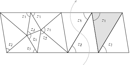
Modulus of three tetrahedra are respectively z1=ep3−p5z_{1}=\mathrm{e}^{p_{3}-p_{5}}, z2=ep5−p4z_{2}=\mathrm{e}^{p_{5}-p_{4}}, and z3=ep2−p6z_{3}=\mathrm{e}^{p_{2}-p_{6}}. The developing map is depicted in Fig. 4. The meridian is read to be z3z2\frac{z_{3}}{z_{2}}, and the condition δC​(𝒑,u)\delta_{C}(\boldsymbol{p};u) is

p5−p4+p6−p2=2​up_{5}-p_{4}+p_{6}-p_{2}=2\,u

We then have

Zγ​(ℳu)=1(4​π​γ)3/2​∬d​x​𝑑y​e12​i​γ​(π2+γ22+32​π​γ+(2​u−y)​(y−x))×1Φγ​(−x+y−2​u−i​π−i​γ)​Φγ​(−y−2​u−i​π−i​γ)​Φγ​(−y−2​u−i​π−i​γ)Z_{\gamma}\left(\mathcal{M}_{u}\right)=\frac{1}{\left(4\,\pi\,\gamma\right)^{3/2}}\,\iint\mathrm{d}x\,\mathrm{d}y\,\mathrm{e}^{\frac{1}{2\mathrm{i}\gamma}\left(\frac{\pi^{2}+\gamma^{2}}{2}+\frac{3}{2}\pi\gamma+(2u-y)(y-x)\right)}\\ \times\frac{1}{\Phi_{\gamma}(-x+y-2\,u-\mathrm{i}\,\pi-\mathrm{i}\,\gamma)\,\Phi_{\gamma}(-y-2\,u-\mathrm{i}\,\pi-\mathrm{i}\,\gamma)\,\Phi_{\gamma}(-y-2\,u-\mathrm{i}\,\pi-\mathrm{i}\,\gamma)} (4.10)
Refer to caption
Figure 4. Developing map of the complement of 525_{2}. Gray filled triangle denotes top vertex of the tetrahedron with modulus z1z_{1}. Meridian is denoted by a gray curve.

In a classical limit γ→0\gamma\to 0, we obtain

Zγ​(ℳu)∼∬d​x​𝑑y​exp⁡(12​i​γ​Vℳ​(ex,ey,eu))Z_{\gamma}\left(\mathcal{M}_{u}\right)\sim\iint\mathrm{d}x\,\mathrm{d}y\,\exp\left(\frac{1}{2\,\mathrm{i}\,\gamma}\,V_{\mathcal{M}}(\mathrm{e}^{x},\mathrm{e}^{y};\mathrm{e}^{u})\right) (4.11)

where the Neumann–Zagier potential function is

Vℳ​(x,y,m)=π22−Li_2⁡(yx​m2)−Li_2⁡(1y​m2)−Li_2⁡(1y)+log⁡(y/x)​log⁡(m2/y)V_{\mathcal{M}}(x,y;m)=\frac{\pi^{2}}{2}-\Li\left(\frac{y}{x\,m^{2}}\right)-\Li\left(\frac{1}{y\,m^{2}}\right)-\Li\left(\frac{1}{y}\right)+\log\left(y/x\right)\,\log\left(m^{2}/y\right) (4.12)

The integral is evaluated by the saddle point method, and saddle point conditions (3.11) which denote hyperbolic consistency conditions reduce to

m2​x−y=x​y(m2​y−1)​(y−1)=m2​(m2​x−y)\begin{gathered}m^{2}\,x-y=x\,y\\[5.69054pt] (m^{2}\,y-1)\,(y-1)=m^{2}\,(m^{2}\,x-y)\end{gathered} (4.13)

and the identity for the longitude (3.12) is given as

m4​y2=(m2​x−y)​(m2​y−1)​ℓm^{4}\,y^{2}=(m^{2}\,x-y)\,(m^{2}\,y-1)\,\ell (4.14)

In the case of complete structure ℳ\mathcal{M}, i.e., u=0u=0, there exists a solution of (4.13), (x,y)=(−0.877439+0.744862​i,0.78492+1.30714​i)(x,y)=(-0.877439+0.744862\,\mathrm{i},0.78492+1.30714\,\mathrm{i}), such that the imaginary part of the potential function

Im⁡Vℳ​(x,y,1)=−D⁡(yx)−2​D​(1y)\operatorname{Im}V_{\mathcal{M}}(x,y;1)=-D\left(\frac{y}{x}\right)-2\,D\left(\frac{1}{y}\right)

gives the hyperbolic volume of ℳ\mathcal{M}; Vol(ℳ)=2.82812⋯\Vol(\mathcal{M})=2.82812\cdots. .

To get the A-polynomial, we eliminate variables xx and yy from a set of equations (4.13) and (4.14). After some algebra we obtain A𝒦​(ℓ,m)=0A_{\mathcal{K}}(\ell,m)=0, where the function A𝒦​(ℓ,m)A_{\mathcal{K}}(\ell,m) coincides with the A-polynomial for 525_{2} given by the following Newton polygon;

(−11−2−2−111−1−2−21−1)\begin{pmatrix}-1&1&&\\ &-2&&\\ &-2&-1&\\ &&1&\\ &1&&\\ &-1&-2&\\ &&-2&\\ &&1&-1\\ \end{pmatrix}

4.3 Pretzel knot (−2,3,7)(-2,3,7)

Let 𝒦\mathcal{K} be the (−2,3,7)(-2,3,7) Pretzel knot depicted as

[Uncaptioned image]

and we set ℳ\mathcal{M} as the complement of 𝒦\mathcal{K}. The Pretzel knot (−2,3,7)(-2,3,7) has the same hyperbolic volume with 525_{2}, Vol(ℳ)=2.82812⋯\Vol(\mathcal{M})=2.82812\cdots, but the triangulations of the complement give the following partition function;

Zγ​(ℳu)=∫ℝd​𝒑​δC​(𝒑,u)​⟨p4,p7​|S|​p6,p1⟩​⟨p5,p8​|S|​p7,p5⟩×⟨p1,p6​|S|​p8,p2⟩​⟨p3,p2​|S|​p4,p3⟩Z_{\gamma}\left(\mathcal{M}_{u}\right)=\int\limits_{\mathbb{R}}\mathrm{d}\boldsymbol{p}\,\delta_{C}(\boldsymbol{p};u)\,\langle p_{4},p_{7}|S|p_{6},p_{1}\rangle\,\langle p_{5},p_{8}|S|p_{7},p_{5}\rangle\\ \times\langle p_{1},p_{6}|S|p_{8},p_{2}\rangle\,\langle p_{3},p_{2}|S|p_{4},p_{3}\rangle (4.15)

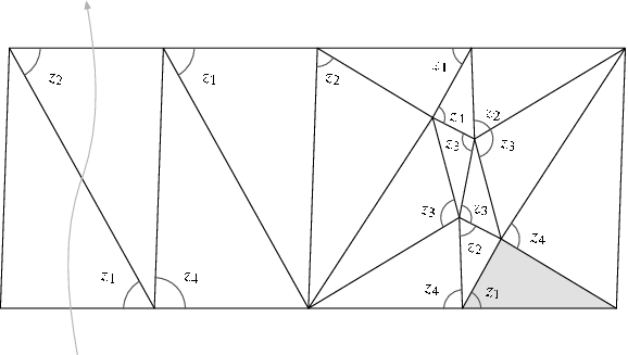
Note that this triangulation differs from the canonical triangulation in Ref. [52]. The developing map is given in Fig. 5. Here we set the modulus of four ideal tetrahedra as

z1\displaystyle z_{1} =ep1−p7\displaystyle=\mathrm{e}^{p_{1}-p_{7}} z2\displaystyle z_{2} =ep5−p8\displaystyle=\mathrm{e}^{p_{5}-p_{8}}
z3\displaystyle z_{3} =ep2−p6\displaystyle=\mathrm{e}^{p_{2}-p_{6}} z4\displaystyle z_{4} =ep3−p2\displaystyle=\mathrm{e}^{p_{3}-p_{2}}

Then the meridian is read as

p2−p6−p1+p7=−2​up_{2}-p_{6}-p_{1}+p_{7}=-2\,u
Refer to caption
Figure 5. Developing map of complement of the Pretzel knot (−2,3,7)(-2,3,7). Horosphere of the top vertex of the tetrahedron with modulus z1z_{1} is depicted by gray triangle. Gray curve denotes a meridian.

In the classical limit of the quantum invariant Zγ​(ℳu)Z_{\gamma}(\mathcal{M}_{u}) we obtain the potential function after some change of variables as

Vℳ​(x,y,z,m)=−2​π23+Li_2⁡(1z)+Li_2⁡(1x​y​z​m4)+Li_2⁡(1z​m2)+Li_2⁡(m2x)+3​(log⁡(m2))2+log⁡(y5x2)​log⁡(m2)+(log⁡x)2+(log⁡y)2V_{\mathcal{M}}(x,y,z;m)=-\frac{2\,\pi^{2}}{3}+\Li\left(\frac{1}{z}\right)+\Li\left(\frac{1}{x\,y\,z\,m^{4}}\right)+\Li\left(\frac{1}{z\,m^{2}}\right)+\Li\left(\frac{m^{2}}{x}\right)\\ +3\left(\log\left(m^{2}\right)\right)^{2}+\log\left(\frac{y^{5}}{x^{2}}\right)\log\left(m^{2}\right)+\left(\log x\right)^{2}+\left(\log y\right)^{2} (4.16)

The hyperbolic consistency conditions (3.11) give

(x​y​z​m4−1)​(x−m2)=y​z​m8y​m6​(x​y​z​m4−1)=x​z(z−1)​(x​y​z​m4−1)​(m2​z−1)=x​y​z3​m6\begin{gathered}\left(x\,y\,z\,m^{4}-1\right)\,\left(x-m^{2}\right)=y\,z\,m^{8}\\[5.69054pt] y\,m^{6}\,\left(x\,y\,z\,m^{4}-1\right)=x\,z\\[5.69054pt] (z-1)\,\left(x\,y\,z\,m^{4}-1\right)\,\left(m^{2}\,z-1\right)=x\,y\,z^{3}\,m^{6}\end{gathered} (4.17)

and the longitude (3.12) is defined by

ℓ=(x​y​z​m4−1)2​(m2​z−1)2​m2​y3(x−m2)​x3​z3\ell=\frac{\left(x\,y\,z\,m^{4}-1\right)^{2}\,\left(m^{2}\,z-1\right)^{2}\,m^{2}\,y^{3}}{\left(x-m^{2}\right)\,x^{3}\,z^{3}} (4.18)

In the complete hyperbolic structure m=1m=1, we have a solution of (4.17),

(xyz)=(0.337641−0.56228​i0.122561+0.744862​i0.618504−0.410401​i)\begin{pmatrix}x\\ y\\ z\end{pmatrix}=\begin{pmatrix}0.337641-0.56228\,\mathrm{i}\\ 0.122561+0.744862\,\mathrm{i}\\ 0.618504-0.410401\,\mathrm{i}\end{pmatrix}

s.t. we recover the hyperbolic volume of 𝒦\mathcal{K};

ImVℳ(x,y,z;m=1)=2D(1/z)+D(1x​y​z)+D(1/x)=2.82812⋯\operatorname{Im}V_{\mathcal{M}}(x,y,z;m=1)=2\,D(1/z)+D\left(\frac{1}{x\,y\,z}\right)+D(1/x)=2.82812\cdots

The A-polynomial is computed by eliminating (x,y,z)(x,y,z) from (4.17) and (4.18), and we obtain A𝒦​(ℓ,m)=0A_{\mathcal{K}}(\ell,m)=0, where the A-polynomial for the (−2,3,7)(-2,3,7) Pretzel knot is

A𝒦​(ℓ,m)=−1+(m16−2​m18+m20)​ℓ+(2​m36+m38)​ℓ2−ℓ4​(m72+2​m74)−ℓ5​(m90−2​m92+m94)+m110​ℓ6A_{\mathcal{K}}(\ell,m)=-1+\left(m^{16}-2\,m^{18}+m^{20}\right)\,\ell+\left(2\,m^{36}+m^{38}\right)\,\ell^{2}\\ -\ell^{4}\,\left(m^{72}+2\,m^{74}\right)-\ell^{5}\,\left(m^{90}-2\,m^{92}+m^{94}\right)+m^{110}\,\ell^{6} (4.19)

4.4 Once-Punctured Torus Bundles over the Circle

One of benefits of the quantum invariant Zγ​(ℳ)Z_{\gamma}(\mathcal{M}) is that we can compute it explicitly for a once-punctured torus bundle over S1S^{1}. A once-punctured torus bundle over S1S^{1}, which we denote ℳ⁡(φ)\mathcal{M}(\varphi), is described by F×[0,1]/(x,0)∼(φ⁡(x),1)F\times[0,1]/(x,0)\sim(\varphi(x),1) where a monodromy matrix φ∈S​L​(2,ℤ)\varphi\in SL(2,\mathbb{Z}) is a homeomorphism from the punctured torus F=𝕋2∖{0}F=\mathbb{T}^{2}\setminus\{0\} to itself. Thurston’s hyperbolization theorem indicates that ℳ⁡(φ)\mathcal{M}(\varphi) admits a complete hyperbolic metric with a finite volume when φ\varphi has 2 distinct real eigenvalues. In this case, the monodromy matrix φ\varphi can be written up to conjugation as

φ=Ls1Rt1⋯LsnRtn\varphi=L^{s_{1}}\,R^{t_{1}}\cdots L^{s_{n}}R^{t_{n}} (4.20)

where

L\displaystyle L =(1101)\displaystyle=\begin{pmatrix}1&1\\ 0&1\end{pmatrix} R\displaystyle R =(1011)\displaystyle=\begin{pmatrix}1&0\\ 1&1\end{pmatrix}

with n>0n>0, and sjs_{j} and tjt_{j} are positive integers. Note that the complement of the figure-eight knot studied in Sec. 4.1 corresponds to φ=L​R=(2111)\varphi=L\,R=\begin{pmatrix}2&1\\ 1&1\end{pmatrix}.

It is known that we can triangulate the manifold MφM_{\varphi} with ∑k=1n(sk+tk)\sum_{k=1}^{n}(s_{k}+t_{k}) ideal tetrahedra [15], and we have the quantum invariant as

Zγ​(ℳu​(φ))=⨌ℝd​𝒂​d𝒃​d𝒄​d𝒅​δC​(𝒂,𝒃,𝒄,𝒅,u)​δG​(𝒂,𝒃,𝒄,𝒅)×∏k=1n[∏i=0sk−1⟨dk,i,ck,i+1|S−1|dk,i+1,ck,i⟩∏j=0tk−1⟨bk,j,ak,j+1|S|bk,j+1,ak,j⟩]Z_{\gamma}\left(\mathcal{M}_{u}(\varphi)\right)=\iiiint\limits_{\mathbb{R}}\mathrm{d}\boldsymbol{a}\,\mathrm{d}\boldsymbol{b}\,\mathrm{d}\boldsymbol{c}\,\mathrm{d}\boldsymbol{d}\,\delta_{C}(\boldsymbol{a},\boldsymbol{b},\boldsymbol{c},\boldsymbol{d};u)\,\delta_{G}(\boldsymbol{a},\boldsymbol{b},\boldsymbol{c},\boldsymbol{d})\\ \times\prod_{k=1}^{n}\left[\prod_{i=0}^{s_{k}-1}\left\langle d_{k,i},c_{k,i+1}\middle|S^{-1}\middle|d_{k,i+1},c_{k,i}\right\rangle\,\prod_{j=0}^{t_{k}-1}\left\langle b_{k,j},a_{k,j+1}\middle|S\middle|b_{k,j+1},a_{k,j}\right\rangle\,\right] (4.21)

where gluing condition δG​(𝒂,𝒃,𝒄,𝒅)\delta_{G}(\boldsymbol{a},\boldsymbol{b},\boldsymbol{c},\boldsymbol{d}) means

{bk,0=ck+1,0ak,0=dk+1,0​for k=1,2,…,n−1\displaystyle\begin{cases}b_{k,0}=c_{k+1,0}\\ a_{k,0}=d_{k+1,0}\end{cases}\text{for $k=1,2,\dots,n-1$} {bn,0=c1,0an,0=d1,0\displaystyle\begin{cases}b_{n,0}=c_{1,0}\\ a_{n,0}=d_{1,0}\end{cases}
{bk,tk=ck,skak,tk=dk,sk​for k=1,2,…,n\displaystyle\begin{cases}b_{k,t_{k}}=c_{k,s_{k}}\\ a_{k,t_{k}}=d_{k,s_{k}}\end{cases}\text{for $k=1,2,\dots,n$}

When we set the modulus of each oriented tetrahedra as

zk,j\displaystyle z_{k,j} =eak,j−ak,j+1\displaystyle=\mathrm{e}^{a_{k,j}-a_{k,j+1}} wk,j\displaystyle w_{k,j} =eck,j−ck,j+1\displaystyle=\mathrm{e}^{c_{k,j}-c_{k,j+1}}

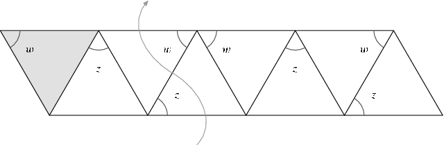
the developing map is drawn schematically as Fig. 6. We can then read a condition δC​(𝒂,𝒃,𝒄,𝒅,u)\delta_{C}(\boldsymbol{a},\boldsymbol{b},\boldsymbol{c},\boldsymbol{d};u) for meridian as

u=12​∑k=1n(ck,0−ck,sk−ak,0+ak,tk)u=\frac{1}{2}\sum_{k=1}^{n}\left(c_{k,0}-c_{k,s_{k}}-a_{k,0}+a_{k,t_{k}}\right) (4.22)

With these conditions, we have the quantum invariant Zγ​(ℳu​(φ))Z_{\gamma}\left(\mathcal{M}_{u}(\varphi)\right), and the Neumann–Zagier potential function can be given by taking a classical limit γ→0\gamma\to 0. As far as we know, the A-polynomial-type invariant for the once-punctured torus bundle over S1S^{1} is not studied, but we can obtain such polynomials from the Neumann–Zagier function.

Below we give a few examples for concreteness.
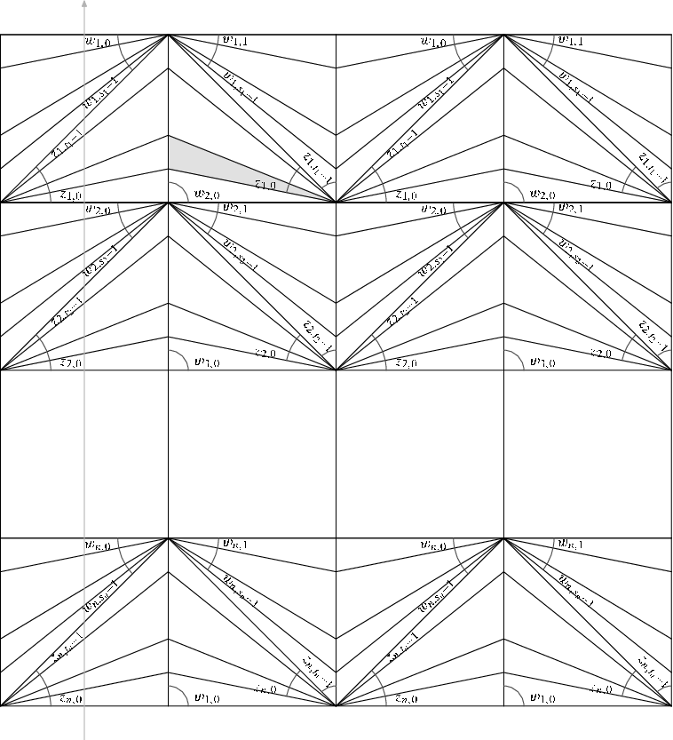
Refer to caption
Figure 6. Schematic developing map for ℳ⁡(φ)\mathcal{M}(\varphi). Top vertex of tetrahedron with modulus z1,0z_{1,0} is filled gray. Gray straight line denotes meridian.

4.4.1 L2​RL^{2}\,R

We set φ=L2​R=(3211)\varphi=L^{2}\,R=\begin{pmatrix}3&2\\ 1&1\end{pmatrix}. The hyperbolic Dehn surgery of this manifold is studied in Ref. [4]. The invariant (4.21) is rewritten as

Zγ​(ℳu​(L2​R))=∫ℝd𝒑δC(𝒑;u)⟨p1,p5|S−1|p6,p3⟩⟨p6,p4|S−1|p2,p5⟩⟨p3,p2|S|p4,p1⟩Z_{\gamma}\left(\mathcal{M}_{u}(L^{2}\,R)\right)\\ =\int\limits_{\mathbb{R}}\mathrm{d}\boldsymbol{p}\,\delta_{C}(\boldsymbol{p};u)\,\left\langle p_{1},p_{5}\middle|S^{-1}\middle|p_{6},p_{3}\right\rangle\,\left\langle p_{6},p_{4}\middle|S^{-1}\middle|p_{2},p_{5}\right\rangle\,\left\langle p_{3},p_{2}\middle|S\middle|p_{4},p_{1}\right\rangle (4.23)

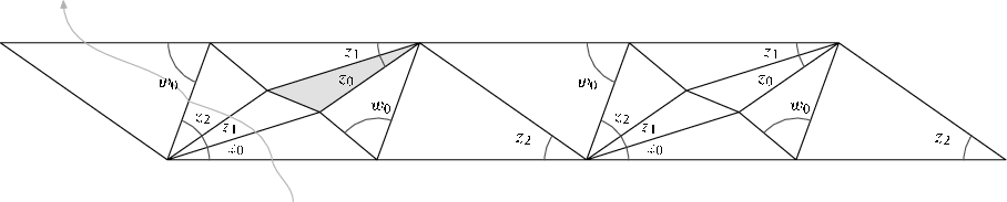
When we set the modulus of tetrahedra as w0=ep3−p5w_{0}=\mathrm{e}^{p_{3}-p_{5}}, w1=ep5−p4w_{1}=\mathrm{e}^{p_{5}-p_{4}}, and z0=ep1−p2z_{0}=\mathrm{e}^{p_{1}-p_{2}}, the developing map ℳ⁡(L2​R)\mathcal{M}(L^{2}\,R) can be depicted as Fig. 7. Then the meridian is read as

p3−p4−p1+p2=2​up_{3}-p_{4}-p_{1}+p_{2}=2\,u (4.24)
Refer to caption
Figure 7. Developing map of ℳ⁡(L2​R)\mathcal{M}(L^{2}\,R). Gray filled triangle is top vertex of the tetrahedron with modulus z0z_{0}. Gray curve is meridian.

In the classical limit, we have

Zγ​(ℳu​(L2​R))∼∬d​x​𝑑y​exp⁡(12​i​γ​Vℳ⁡(L2​R)​(ex,ey,eu))Z_{\gamma}\left(\mathcal{M}_{u}(L^{2}\,R)\right)\sim\iint\mathrm{d}x\,\mathrm{d}y\,\exp\left(\frac{1}{2\,\mathrm{i}\,\gamma}\,V_{\mathcal{M}(L^{2}R)}(\mathrm{e}^{x},\mathrm{e}^{y};\mathrm{e}^{u})\right) (4.25)

where the potential function is computed as

Vℳ⁡(L2​R)​(x,y,m)=Li_2⁡(1m2​x)−Li_2⁡(1m2​x​y2)−Li_2⁡(m2​x2​y2)−log⁡(m2)​log⁡(m2​x2​y4)−2​(log⁡(x​y))2+π26V_{\mathcal{M}(L^{2}R)}(x,y;m)=\Li\left(\frac{1}{m^{2}\,x}\right)-\Li\left(\frac{1}{m^{2}\,x\,y^{2}}\right)-\Li\left(m^{2}\,x^{2}\,y^{2}\right)\\ -\log\left(m^{2}\right)\log\left(m^{2}\,x^{2}\,y^{4}\right)-2\left(\log\left(x\,y\right)\right)^{2}+\frac{\pi^{2}}{6} (4.26)

The saddle point conditions (3.11), which correspond to the hyperbolic consistency condition, reduce to

(−1+m2​x)​(−1+m2​x2​y2)2m4​x4​y2​(−1+m2​x​y2)=1(−1+m2​x2​y2)m2​x​(−1+m2​x​y2)=1\begin{gathered}\frac{\left(-1+m^{2}\,x\right)\,\left(-1+m^{2}\,x^{2}\,y^{2}\right)^{2}}{m^{4}\,x^{4}\,y^{2}\,\left(-1+m^{2}\,x\,y^{2}\right)}=1\\[5.69054pt] \frac{\left(-1+m^{2}\,x^{2}\,y^{2}\right)}{m^{2}\,x\,\left(-1+m^{2}\,x\,y^{2}\right)}=1\end{gathered} (4.27)

and, as (3.12), the longitude is defined by

ℓ=−(−1+m2​x)​(−1+m2​x2​y2)m4​x2​y2​(−1+m2​x​y2)\ell=-\frac{(-1+m^{2}\,x)\,(-1+m^{2}\,x^{2}\,y^{2})}{m^{4}\,x^{2}\,y^{2}\,(-1+m^{2}\,x\,y^{2})} (4.28)

In the case of complete case m=1m=1, we find that (x,y2)=(1±7​i4,−1±7​i2)(x,y^{2})=\left(\frac{1\pm\sqrt{7}\,\mathrm{i}}{4},\frac{-1\pm\sqrt{7}\,\mathrm{i}}{2}\right) solves the consistency condition (4.27). Among these, we can check numerically that the largest value of the imaginary part of the potential function at the saddle points

Im⁡Vℳ⁡(L2​R)​(x,y,m=1)=D⁡(1x)−D⁡(1x​y2)−D⁡(x2​y2)\operatorname{Im}V_{\mathcal{M}(L^{2}R)}(x,y;m=1)=D\left(\frac{1}{x}\right)-D\left(\frac{1}{x\,y^{2}}\right)-D\left(x^{2}\,y^{2}\right)

coincides with the hyperbolic volume Vol(ℳ(L2R))=2.66674⋯\Vol\left(\mathcal{M}(L^{2}\,R)\right)=2.66674\cdots.

The A-polynomial is now given by eliminating xx and yy from the set of equations, (4.27) and (4.28), and we obtain the algebraic curve Aℳ⁡(L2​R)​(ℓ,m)=0A_{\mathcal{M}(L^{2}R)}(\ell,m)=0 whose Newton polygon is given by

(0−100211200−10)\begin{pmatrix}0&-1&0\\ 0&2&1\\ 1&2&0\\ 0&-1&0\end{pmatrix}

4.4.2 L​R3L\,R^{3}

We take another example φ=L​R3=(4131)\varphi=L\,R^{3}=\begin{pmatrix}4&1\\ 3&1\end{pmatrix}. In this case, the invariant (4.21) becomes

Zγ(ℳu(LR3))=∫ℝd𝒑δC(𝒑;u)⟨p1,p4|S|p3,p2⟩⟨p3,p6|S|p5,p4⟩×⟨p5,p8|S|p7,p6⟩⟨p2,p7|S−1|p8,p1⟩Z_{\gamma}(\mathcal{M}_{u}(L\,R^{3}))=\int\limits_{\mathbb{R}}\mathrm{d}\boldsymbol{p}\,\delta_{C}(\boldsymbol{p};u)\,\left\langle p_{1},p_{4}\middle|S\middle|p_{3},p_{2}\right\rangle\,\left\langle p_{3},p_{6}\middle|S\middle|p_{5},p_{4}\right\rangle\\ \times\left\langle p_{5},p_{8}\middle|S\middle|p_{7},p_{6}\right\rangle\,\left\langle p_{2},p_{7}\middle|S^{-1}\middle|p_{8},p_{1}\right\rangle (4.29)

We set the modulus of each tetrahedron as

z0\displaystyle z_{0} =ep2−p4\displaystyle=\mathrm{e}^{p_{2}-p_{4}} z1\displaystyle z_{1} =ep4−p6\displaystyle=\mathrm{e}^{p_{4}-p_{6}}
z2\displaystyle z_{2} =ep6−p8\displaystyle=\mathrm{e}^{p_{6}-p_{8}} w0\displaystyle w_{0} =ep1−p7\displaystyle=\mathrm{e}^{p_{1}-p_{7}}

The developing map is depicted in Fig. 8, and the meridian is read as w0z0​z1​z2\frac{w_{0}}{z_{0}\,z_{1}\,z_{2}}. We thus have a condition of δC​(𝒑,u)\delta_{C}(\boldsymbol{p};u) as

p1−p7−p2+p8=2​up_{1}-p_{7}-p_{2}+p_{8}=2\,u (4.30)
Refer to caption
Figure 8. Developing map of ℳ⁡(L​R3)\mathcal{M}(L\,R^{3}).

In the classical limit, we obtain

Zγ​(ℳu​(L​R3))∼∭d​x​𝑑y​𝑑z​exp⁡(12​i​γ​Vℳ⁡(L​R3)​(ex,ey,ez,eu))Z_{\gamma}(\mathcal{M}_{u}(L\,R^{3}))\sim\iiint\mathrm{d}x\,\mathrm{d}y\,\mathrm{d}z\,\exp\left(\frac{1}{2\,\mathrm{i}\,\gamma}\,V_{\mathcal{M}(LR^{3})}(\mathrm{e}^{x},\mathrm{e}^{y},\mathrm{e}^{z};\mathrm{e}^{u})\right) (4.31)

where the potential function is computed as

Vℳ⁡(L​R3)​(x,y,z,m)=−Li_2⁡(1m4​y)+Li_2⁡(1m2​x​y​z2)+Li_2⁡(m2​x2​z)+Li_2⁡(m2​y2​zx)−(log⁡(m2))2+2​log⁡(xm2)​log⁡(xy)+2​log⁡y​log⁡(y​z)+2​log⁡z​log⁡(x​z​m2)−π23V_{\mathcal{M}(LR^{3})}(x,y,z;m)=-\Li\left(\frac{1}{m^{4}\,y}\right)+\Li\left(\frac{1}{m^{2}\,x\,y\,z^{2}}\right)+\Li\left(m^{2}\,x^{2}\,z\right)\\ +\Li\left(\frac{m^{2}\,y^{2}\,z}{x}\right)-\left(\log\left(m^{2}\right)\right)^{2}+2\log\left(\frac{x}{m^{2}}\right)\log\left(\frac{x}{y}\right)\\ +2\log y\log(y\,z)+2\log z\log(x\,z\,m^{2})-\frac{\pi^{2}}{3} (4.32)

In the case of complete case m=1m=1, we can check numerically that among algebraic solutions of (3.11) the maximum of the imaginary part of Vℳ⁡(L​R3)​(x,y,z,m=1)V_{\mathcal{M}(LR^{3})}(x,y,z;m=1),

Im⁡Vℳ⁡(L​R3)​(x,y,z,1)=−D⁡(1y)+D⁡(1x​y​z2)+D⁡(x2​z)+D⁡(y2​zx)\operatorname{Im}V_{\mathcal{M}(LR^{3})}(x,y,z;1)=-D\left(\frac{1}{y}\right)+D\left(\frac{1}{x\,y\,z^{2}}\right)+D\left(x^{2}\,z\right)+D\left(\frac{y^{2}\,z}{x}\right)

coincides with the hyperbolic volume Vol(ℳ(LR3))=2.98912⋯\Vol(\mathcal{M}(L\,R^{3}))=2.98912\cdots. See Ref. [16] where algebraic solutions of consistency equations are investigated in detail.

Correspondingly we obtain the A-polynomial for ℳ⁡(L​R3)\mathcal{M}(L\,R^{3}) by eliminating xx, yy, and zz from a set of equations. Explicitly the polynomial Aℳ⁡(L​R3)​(ℓ,m)A_{\mathcal{M}(LR^{3})}(\ell,m) is given in the form of Newton polygon as follows;

(000100000−300−1−2−3−1−200−3−223002132100300000−1000)\begin{pmatrix}0&0&0&1&0&0\\ 0&0&0&-3&0&0\\ -1&-2&-3&-1&-2&0\\ 0&-3&-2&2&3&0\\ 0&2&1&3&2&1\\ 0&0&3&0&0&0\\ 0&0&-1&0&0&0\end{pmatrix}

5. Conclusion and Discussion

We have constructed quantum invariant Zγ​(ℳ)Z_{\gamma}(\mathcal{M}) for cusped hyperbolic 3-manifolds ℳ\mathcal{M} by assigning the Faddeev quantum dilogarithm function to oriented ideal tetrahedra. Once the triangulation of cusped 3-manifold ℳ\mathcal{M} is given, it is rather straightforward to define the invariant Zγ​(ℳ)Z_{\gamma}(\mathcal{M}) in an integral form. In the classical limit, the Faddeev integral reduces to the dilogarithm function, which denotes the hyperbolic volume of ideal tetrahedron. Remarkable is that the saddle point conditions coincide with the hyperbolic consistency conditions around edges [19]. We have discussed as a variant of the volume conjecture that the invariant Zγ​(ℳ)Z_{\gamma}(\mathcal{M}), which can be regarded as a generalization of the Kashaev invariant (specific value of the colored Jones polynomial), is dominated by the hyperbolic volume in the classical limit γ→0\gamma\to 0.

We have shown that the invariant can be defined for a one-parameter deformation of manifold ℳu\mathcal{M}_{u} (not complete), and that the Neumann–Zagier potential function can be given by taking a classical limit γ→0\gamma\to 0. Correspondingly the A-polynomial can be computed from the potential function (3.14). This supports the generalized volume conjecture. We have demonstrated by taking examples that our method recovers previously known A-polynomial when ℳ\mathcal{M} is a complement of hyperbolic knots. We have further applied our method in the case of the once-punctured torus bundle over the circle. It seems that the A-polynomial-type invariant is not known for this 3-manifold, and it will be interesting to study a relationship with the boundary slope. To conclude, our results indicate that the SS-operator (2.13) denotes the quantum Bloch invariant for oriented ideal tetrahedron.

The A-polynomial may give an interesting insight for mathematical physics. For example, the Mahler measure of the A-polynomial is expected to coincide with the hyperbolic volume of knot. On the other hand, the Mahler measure of the determinant of the Kasteleyn matrix has appeared as the free energy of the dimer problem. From the viewpoint of our combinatorial construction of the quantum invariant, the quantum invariants based on oriented ideal triangulation may be interpreted as a matching of in-states and out-states, and it might be interesting to investigate a Kasteleyn matrix interpretation of the A-polynomial.

Acknowledgments

We have used computer programs, SnapPea [52], Knotscape [24], and Snap [11], in studying triangulation of manifolds. We have also used Mathematica and Pari/GP. Pictures of knots in this paper are drawn using KnotPlot [47]. This work is supported in part by Grant-in-Aid for Young Scientists from the Ministry of Education, Culture, Sports, Science and Technology of Japan.

Appendix A More Examples

We shall study the quantum invariant for other cusped manifolds. We give

  • •

    the quantum invariant Zγ​(ℳ)Z_{\gamma}(\mathcal{M}) in terms of the SS-operators,

  • •

    developing map when the number of the ideal tetrahedron is less than four,

  • •

    the condition δC​(𝒑,u)\delta_{C}(\boldsymbol{p};u), where uu is a deformation parameter from the completeness u=0u=0,

  • •

    the Neumann–Zagier potential function Vℳ​(𝒙,m)V_{\mathcal{M}}(\boldsymbol{x};m), which follows from Zγ​(ℳ)Z_{\gamma}(\mathcal{M}) by taking the classical limit γ→0\gamma\to 0,

  • •

    a solution of the saddle point equations in the complete case u=0u=0, which is checked that the hyperbolic volume coincides with a maximal value of the imaginary part of the potential function at this saddle point,

  • •

    the A-polynomial, which is given from the potential function Vℳ​(𝒙,m)V_{\mathcal{M}}(\boldsymbol{x};m) by eliminating parameters 𝒙\boldsymbol{x}.

In the first part A.1, we collect results for hyperbolic knots up to 7 crossings. Though the A-polynomial is given in Ref. [9], we give an explicit form for self-completeness. In the second part A.2, we consider simple hyperbolic knots K​xyK\,x_{y} from Ref. [6]. Pictures of knot may be complicated, but the triangulation of the complement is relatively simple in these cases. We note that, though the number of the ideal tetrahedra of the complement of knot K​xyK\,x_{y} is xx in the case of the canonical triangulation [52], our triangulations are different.

A.1 Complement of Knots up to 7 Crossings

A.1.1 616_{1}

[Uncaptioned image] Vol⁡(S3∖𝒦)=3.16396​…\displaystyle\Vol(S^{3}\setminus\mathcal{K})=3.16396\dots
  • •

    Quantum invariant

    Zγ​(ℳu)=∫ℝd​𝒑​δC​(𝒑,u)​⟨p3,p1​|S−1|​p2,p4⟩​⟨p6,p4​|S|​p5,p8⟩×⟨p7,p5​|S−1|​p6,p1⟩​⟨p8,p2​|S|​p7,p3⟩Z_{\gamma}\left(\mathcal{M}_{u}\right)=\int\limits_{\mathbb{R}}\mathrm{d}\boldsymbol{p}\,\delta_{C}(\boldsymbol{p};u)\,\langle p_{3},p_{1}|S^{-1}|p_{2},p_{4}\rangle\,\langle p_{6},p_{4}|S|p_{5},p_{8}\rangle\\ \times\langle p_{7},p_{5}|S^{-1}|p_{6},p_{1}\rangle\,\langle p_{8},p_{2}|S|p_{7},p_{3}\rangle
  • •

    Developing map (Fig. 9)

    Refer to caption
    Figure 9. Developing map of the knot complement of 616_{1}. Gray triangle is a horosphere of the top vertex of the tetrahedron with modulus z1z_{1}, where we have set z1=ep4−p1z_{1}=\mathrm{e}^{p_{4}-p_{1}} , z2=ep8−p4z_{2}=\mathrm{e}^{p_{8}-p_{4}}, z3=ep1−p5z_{3}=\mathrm{e}^{p_{1}-p_{5}}, and z4=ep3−p2z_{4}=\mathrm{e}^{p_{3}-p_{2}}.
  • •

    Condition δC​(𝒑,u)\delta_{C}(\boldsymbol{p};u)

    p4−p1−p3+p2=2​up_{4}-p_{1}-p_{3}+p_{2}=2\,u
  • •

    Potential function

    Vℳ​(x,y,z,m)=Li_2⁡(z​m2x​y)+Li_2⁡(y)−Li_2⁡(m2y)−Li_2⁡(y​zm2)+log⁡(m2)​log⁡(y​z2x)−log⁡z​log⁡(x​y)V_{\mathcal{M}}(x,y,z;m)=\Li\left(\frac{z\,m^{2}}{x\,y}\right)+\Li(y)-\Li\left(\frac{m^{2}}{y}\right)-\Li\left(\frac{y\,z}{m^{2}}\right)\\ +\log\left(m^{2}\right)\,\log\left(\frac{y\,z^{2}}{x}\right)-\log z\,\log(x\,y)
  • •

    Hyperbolic volume

    Vol⁡(ℳ)=Im⁡Vℳ​(x,y,z,m=1)=D⁡(zx​y)+D⁡(y)−D⁡(1y)−D⁡(y​z)\Vol(\mathcal{M})=\operatorname{Im}V_{\mathcal{M}}(x,y,z;m=1)=D\left(\frac{z}{x\,y}\right)+D(y)-D\left(\frac{1}{y}\right)-D\left({y\,z}\right)

    where

    (xyz)=(−0.851808+0.911292​i0.278726+0.48342​i−1.50411−1.22685​i)\displaystyle\begin{pmatrix}x\\ y\\ z\end{pmatrix}=\begin{pmatrix}-0.851808+0.911292\,\mathrm{i}\\ 0.278726+0.48342\,\mathrm{i}\\ -1.50411-1.22685\,\mathrm{i}\end{pmatrix}
  • •

    A-polynomial

    (00−110003−10021000−3−300−1−3−6−3−100−3−30001200−130001−100)\begin{pmatrix}0&0&-1&1&0\\ 0&0&3&-1&0\\ 0&2&1&0&0\\ 0&-3&-3&0&0\\ -1&-3&-6&-3&-1\\ 0&0&-3&-3&0\\ 0&0&1&2&0\\ 0&-1&3&0&0\\ 0&1&-1&0&0\end{pmatrix}

A.1.2 626_{2}

[Uncaptioned image] Vol⁡(S3∖𝒦)=4.40083​…\displaystyle\Vol(S^{3}\setminus\mathcal{K})=4.40083\dots
  • •

    Quantum invariant

    Zγ​(ℳu)=∫ℝd​𝒑​δC​(𝒑,u)​⟨p8,p6​|S−1|​p1,p2⟩​⟨p3,p7​|S−1|​p8,p4⟩×⟨p4,p5​|S|​p3,p9⟩​⟨p2,p10​|S|​p6,p5⟩​⟨p1,p9​|S−1|​p10,p7⟩Z_{\gamma}\left(\mathcal{M}_{u}\right)=\int\limits_{\mathbb{R}}\mathrm{d}\boldsymbol{p}\,\delta_{C}(\boldsymbol{p};u)\,\langle p_{8},p_{6}|S^{-1}|p_{1},p_{2}\rangle\,\langle p_{3},p_{7}|S^{-1}|p_{8},p_{4}\rangle\,\\ \times\langle p_{4},p_{5}|S|p_{3},p_{9}\rangle\,\langle p_{2},p_{10}|S|p_{6},p_{5}\rangle\,\langle p_{1},p_{9}|S^{-1}|p_{10},p_{7}\rangle
  • •

    Condition δC​(𝒑,u)\delta_{C}(\boldsymbol{p};u)

    p2−p6−p5+p10=−2​up_{2}-p_{6}-p_{5}+p_{10}=-2\,u
  • •

    Potential function

    Vℳ​(w,x,y,z,m)=Li_2⁡(zm2)+Li_2⁡(m4y​w)−Li_2⁡(y​wm2)−Li_2⁡(m2x​y)−Li_2⁡(y​zm2)+log⁡x​log⁡z−log⁡(y​w)​log⁡(y​z)+log⁡(m2)​log⁡(y2​zw)V_{\mathcal{M}}(w,x,y,z;m)=\Li\left(\frac{z}{m^{2}}\right)+\Li\left(\frac{m^{4}}{y\,w}\right)-\Li\left(\frac{y\,w}{m^{2}}\right)-\Li\left(\frac{m^{2}}{x\,y}\right)-\Li\left(\frac{y\,z}{m^{2}}\right)\\ +\log x\,\log z-\log(y\,w)\,\log(y\,z)+\log\left(m^{2}\right)\,\log\left(\frac{y^{2}\,z}{w}\right)
  • •

    Hyperbolic volume

    Im⁡Vℳ​(w,x,y,z,1)=D⁡(z)+D⁡(1y​w)−D⁡(y​w)−D⁡(1x​y)−D⁡(y​z)\operatorname{Im}V_{\mathcal{M}}(w,x,y,z;1)=D\left({z}\right)+D\left(\frac{1}{y\,w}\right)-D\left(y\,w\right)-D\left(\frac{1}{x\,y}\right)-D\left(y\,z\right)

    with

    (wxyz)=(−0.455697+1.20015​i−0.964913−0.621896​i−0.418784−0.219165​i0.0904327+1.60288​i)\begin{pmatrix}w\\ x\\ y\\ z\\ \end{pmatrix}=\begin{pmatrix}-0.455697+1.20015\,\mathrm{i}\\ -0.964913-0.621896\,\mathrm{i}\\ -0.418784-0.219165\,\mathrm{i}\\ 0.0904327+1.60288\,\mathrm{i}\end{pmatrix}
  • •

    A-polynomial

    (0100000−21000−11−30000210000−550000−53−30003−1280000−13300003−1300008−123000−33−500005−50000120000−31−10001−20000010)\begin{pmatrix}0&1&0&0&0&0\\ 0&-2&1&0&0&0\\ -1&1&-3&0&0&0\\ 0&2&1&0&0&0\\ 0&-5&5&0&0&0\\ 0&-5&3&-3&0&0\\ 0&3&-12&8&0&0\\ 0&0&-13&3&0&0\\ 0&0&3&-13&0&0\\ 0&0&8&-12&3&0\\ 0&0&-3&3&-5&0\\ 0&0&0&5&-5&0\\ 0&0&0&1&2&0\\ 0&0&0&-3&1&-1\\ 0&0&0&1&-2&0\\ 0&0&0&0&1&0\end{pmatrix}

A.1.3 636_{3}

[Uncaptioned image] Vol⁡(S3∖𝒦)=5.69302​…\displaystyle\Vol(S^{3}\setminus\mathcal{K})=5.69302\dots
  • •

    Quantum invariant

    Zγ​(ℳu)=∫ℝd​𝒑​δC​(𝒑,u)​⟨p3,p2​|S|​p1,p9⟩​⟨p7,p9​|S−1|​p5,p10⟩​⟨p10,p4​|S−1|​p6,p8⟩×⟨p8,p1​|S−1|​p4,p11⟩​⟨p12,p11​|S−1|​p2,p3⟩​⟨p6,p5​|S|​p12,p7⟩Z_{\gamma}\left(\mathcal{M}_{u}\right)=\int\limits_{\mathbb{R}}\mathrm{d}\boldsymbol{p}\,\delta_{C}(\boldsymbol{p};u)\,\langle p_{3},p_{2}|S|p_{1},p_{9}\rangle\,\langle p_{7},p_{9}|S^{-1}|p_{5},p_{10}\rangle\,\langle p_{10},p_{4}|S^{-1}|p_{6},p_{8}\rangle\\ \times\langle p_{8},p_{1}|S^{-1}|p_{4},p_{11}\rangle\,\langle p_{12},p_{11}|S^{-1}|p_{2},p_{3}\rangle\,\langle p_{6},p_{5}|S|p_{12},p_{7}\rangle (A.1)
  • •

    Condition δC​(𝒑,u)\delta_{C}(\boldsymbol{p};u)

    p10−p9−p7+p5=−2​up_{10}-p_{9}-p_{7}+p_{5}=-2\,u
  • •

    Potential function

    Vℳ​(v,w,x,y,z,m)=Li_2⁡(m2​yx)+Li_2⁡(vw)−Li_2⁡(m2​wv)−Li_2⁡(x​zv)−Li_2⁡(x2​zv)−Li_2⁡(vx​y​z)+π23+log⁡(m2)​log⁡(yw)+log⁡x​log⁡(vy​z2)+log⁡(wy​z)​log⁡(zv)V_{\mathcal{M}}(v,w,x,y,z;m)\\ =\Li\left(\frac{m^{2}\,y}{x}\right)+\Li\left(\frac{v}{w}\right)-\Li\left(\frac{m^{2}\,w}{v}\right)-\Li\left(\frac{x\,z}{v}\right)-\Li\left(\frac{x^{2}\,z}{v}\right)-\Li\left(\frac{v}{x\,y\,z}\right)\\ +\frac{\pi^{2}}{3}+\log\left(m^{2}\right)\,\log\left(\frac{y}{w}\right)+\log x\,\log\left(\frac{v}{y\,z^{2}}\right)+\log\left(\frac{w}{y\,z}\right)\log\left(\frac{z}{v}\right)
  • •

    Hyperbolic volume

    Im⁡Vℳ​(v,w,x,y,z,1)=D⁡(yx)+D⁡(vw)−D⁡(wv)−D⁡(x​zv)−D⁡(x2​zv)−D⁡(vx​y​z)\operatorname{Im}V_{\mathcal{M}}(v,w,x,y,z;1)=D\left(\frac{y}{x}\right)+D\left(\frac{v}{w}\right)-D\left(\frac{w}{v}\right)-D\left(\frac{x\,z}{v}\right)-D\left(\frac{x^{2}\,z}{v}\right)-D\left(\frac{v}{x\,y\,z}\right)

    with

    (vwxyz)=(0.0739495+0.558752​i0.732786+0.381252​i1.00.108378+0.818891​i0.415113+0.381252​i)\begin{pmatrix}v\\ w\\ x\\ y\\ z\end{pmatrix}=\begin{pmatrix}0.0739495+0.558752\,\mathrm{i}\\ 0.732786+0.381252\,\mathrm{i}\\ 1.0\\ 0.108378+0.818891\,\mathrm{i}\\ 0.415113+0.381252\,\mathrm{i}\end{pmatrix}
  • •

    A-polynomial

    (0001000001−510000−43−4000049400022−22200−5−6−21−6−50012821011017341710101282100−5−6−21−6−50022−2220004940000−43−400001−51000001000)\begin{pmatrix}0&0&0&1&0&0&0\\ 0&0&1&-5&1&0&0\\ 0&0&-4&3&-4&0&0\\ 0&0&4&9&4&0&0\\ 0&2&2&-2&2&2&0\\ 0&-5&-6&-21&-6&-5&0\\ 0&1&2&8&2&1&0\\ 1&10&17&34&17&10&1\\ 0&1&2&8&2&1&0\\ 0&-5&-6&-21&-6&-5&0\\ 0&2&2&-2&2&2&0\\ 0&0&4&9&4&0&0\\ 0&0&-4&3&-4&0&0\\ 0&0&1&-5&1&0&0\\ 0&0&0&1&0&0&0\end{pmatrix}

A.1.4 727_{2}

[Uncaptioned image] Vol⁡(S3∖𝒦)=3.33174​…\displaystyle\Vol(S^{3}\setminus\mathcal{K})=3.33174\dots
  • •

    Quantum invariant

    Zγ​(ℳu)=∫ℝd​𝒑​δC​(𝒑,u)​⟨p1,p4​|S|​p2,p3⟩​⟨p5,p2​|S|​p8,p1⟩×⟨p8,p7​|S−1|​p7,p6⟩​⟨p6,p3​|S|​p4,p5⟩Z_{\gamma}\left(\mathcal{M}_{u}\right)=\int\limits_{\mathbb{R}}\mathrm{d}\boldsymbol{p}\,\delta_{C}(\boldsymbol{p};u)\,\langle p_{1},p_{4}|S|p_{2},p_{3}\rangle\,\langle p_{5},p_{2}|S|p_{8},p_{1}\rangle\\ \times\langle p_{8},p_{7}|S^{-1}|p_{7},p_{6}\rangle\,\langle p_{6},p_{3}|S|p_{4},p_{5}\rangle
  • •

    Developing map (Fig. 10)

    Refer to caption
    Figure 10. Developing map of the knot complement of 727_{2}. The gray triangle corresponds to top vertex of the tetrahedron with modulus z1z_{1}, where we have set modulus as z1=ep3−p4z_{1}=\mathrm{e}^{p_{3}-p_{4}} , z2=ep1−p2z_{2}=\mathrm{e}^{p_{1}-p_{2}}, z3=ep6−p7z_{3}=\mathrm{e}^{p_{6}-p_{7}}, and z4=ep5−p3z_{4}=\mathrm{e}^{p_{5}-p_{3}}.
  • •

    Condition δC​(𝒑,u)\delta_{C}(\boldsymbol{p};u)

    p3−p4−p1+p2=−2​up_{3}-p_{4}-p_{1}+p_{2}=-2\,u
  • •

    Potential function

    Vℳ​(x,y,z,m)=Li_2⁡(1x)+Li_2⁡(m2x)+Li_2⁡(z​m2)−Li_2⁡(y​zx2)−π23−(log⁡(x/y))2+log⁡z​log⁡(x3​m2y2​z)V_{\mathcal{M}}(x,y,z;m)=\Li\left(\frac{1}{x}\right)+\Li\left(\frac{m^{2}}{x}\right)+\Li\left(z\,m^{2}\right)-\Li\left(\frac{y\,z}{x^{2}}\right)-\frac{\pi^{2}}{3}\\ -\left(\log(x/y)\right)^{2}+\log z\,\log\left(\frac{x^{3}\,m^{2}}{y^{2}\,z}\right)
  • •

    Hyperbolic volume

    Im⁡Vℳ​(x,y,z,1)=2​D​(1x)+D⁡(z)−D⁡(y​zx2)\operatorname{Im}V_{\mathcal{M}}(x,y,z;1)=2\,D\left(\frac{1}{x}\right)+D\left(z\right)-D\left(\frac{y\,z}{x^{2}}\right)

    with

    (xyz)=(0.941819−1.69128​i0.935538+0.903908​i0.0581814+1.69128​i)\begin{pmatrix}x\\ y\\ z\end{pmatrix}=\begin{pmatrix}0.941819-1.69128\,\mathrm{i}\\ 0.935538+0.903908\,\mathrm{i}\\ 0.0581814+1.69128\,\mathrm{i}\end{pmatrix}
  • •

    A-polynomial

    (1−2100004−4000032−200005500006110000−4−100−1−400001160000550000−2230000−4400001−21)\begin{pmatrix}1&-2&1&0&0&0\\ 0&4&-4&0&0&0\\ 0&3&2&-2&0&0\\ 0&0&5&5&0&0\\ 0&0&6&1&1&0\\ 0&0&0&-4&-1&0\\ 0&-1&-4&0&0&0\\ 0&1&1&6&0&0\\ 0&0&5&5&0&0\\ 0&0&-2&2&3&0\\ 0&0&0&-4&4&0\\ 0&0&0&1&-2&1\\ \end{pmatrix}

A.1.5 737_{3}

[Uncaptioned image] Vol⁡(S3∖𝒦)=4.5921​…\displaystyle\Vol(S^{3}\setminus\mathcal{K})=4.5921\dots
  • •

    Quantum invariant

    Zγ​(ℳu)=∫ℝd​𝒑​δC​(𝒑,u)​⟨p1,p3​|S|​p4,p8⟩​⟨p2,p8​|S|​p5,p1⟩×⟨p5,p9​|S−1|​p6,p7⟩​⟨p4,p6​|S|​p3,p10⟩​⟨p7,p10​|S|​p2,p9⟩Z_{\gamma}\left(\mathcal{M}_{u}\right)=\int\limits_{\mathbb{R}}\mathrm{d}\boldsymbol{p}\,\delta_{C}(\boldsymbol{p};u)\,\langle p_{1},p_{3}|S|p_{4},p_{8}\rangle\,\langle p_{2},p_{8}|S|p_{5},p_{1}\rangle\\ \times\langle p_{5},p_{9}|S^{-1}|p_{6},p_{7}\rangle\,\langle p_{4},p_{6}|S|p_{3},p_{10}\rangle\,\langle p_{7},p_{10}|S|p_{2},p_{9}\rangle
  • •

    Condition δC​(𝒑,u)\delta_{C}(\boldsymbol{p};u)

    p10−p6−p1+p8=−2​up_{10}-p_{6}-p_{1}+p_{8}=-2\,u
  • •

    Potential function

    Vℳ​(w,x,y,z,m)=Li_2⁡(m2​w)+Li_2⁡(m4​w)+Li_2⁡(1m2​x)+Li_2⁡(zw)−Li_2⁡(zy)−π22+log⁡w​log​x+log⁡y​log​z+log⁡(m2)​log⁡(y​w2​z)V_{\mathcal{M}}(w,x,y,z;m)=\Li\left(m^{2}\,w\right)+\Li(m^{4}\,w)+\Li\left(\frac{1}{m^{2}\,x}\right)+\Li\left(\frac{z}{w}\right)-\Li\left(\frac{z}{y}\right)-\frac{\pi^{2}}{2}\\ +\log w\,\log x+\log y\,\log z+\log\left(m^{2}\right)\,\log(y\,w^{2}\,z)
  • •

    Hyperbolic volume

    Im⁡Vℳ​(w,x,y,z,1)=2​D​(w)+D⁡(1x)+D⁡(zw)−D⁡(zy)\operatorname{Im}V_{\mathcal{M}}(w,x,y,z;1)=2\,D\left(w\right)+D\left(\frac{1}{x}\right)+D\left(\frac{z}{w}\right)-D\left(\frac{z}{y}\right)

    with

    (xyzw)=(0.645284−0.801205​i−0.676708+0.260961​i−0.87287+1.51178​i0.537981+1.04357​i)\begin{pmatrix}x\\ y\\ z\\ w\end{pmatrix}=\begin{pmatrix}0.645284-0.801205\,\mathrm{i}\\ -0.676708+0.260961\,\mathrm{i}\\ -0.87287+1.51178\,\mathrm{i}\\ 0.537981+1.04357\,\mathrm{i}\end{pmatrix}
  • •

    A-polynomial

    (−11000000−200000010000000000000−5−300000−29000003−200000−2−14000000−23000004−1000000−4300000−21200000−3−6−1000032430000−1−6−30000012−2000003−400000−104000003−2000000−14−200000−23000009−200000−3−500000000000001000000−20000001−1)\begin{pmatrix}-1&1&0&0&0&0&0\\ 0&-2&0&0&0&0&0\\ 0&1&0&0&0&0&0\\ 0&0&0&0&0&0&0\\ 0&-5&-3&0&0&0&0\\ 0&-2&9&0&0&0&0\\ 0&3&-2&0&0&0&0\\ 0&-2&-14&0&0&0&0\\ 0&0&-2&3&0&0&0\\ 0&0&4&-10&0&0&0\\ 0&0&-4&3&0&0&0\\ 0&0&-2&12&0&0&0\\ 0&0&-3&-6&-1&0&0\\ 0&0&3&24&3&0&0\\ 0&0&-1&-6&-3&0&0\\ 0&0&0&12&-2&0&0\\ 0&0&0&3&-4&0&0\\ 0&0&0&-10&4&0&0\\ 0&0&0&3&-2&0&0\\ 0&0&0&0&-14&-2&0\\ 0&0&0&0&-2&3&0\\ 0&0&0&0&9&-2&0\\ 0&0&0&0&-3&-5&0\\ 0&0&0&0&0&0&0\\ 0&0&0&0&0&1&0\\ 0&0&0&0&0&-2&0\\ 0&0&0&0&0&1&-1\end{pmatrix}

A.1.6 747_{4}

[Uncaptioned image] Vol(S3∖𝒦)=5.13794⋯\displaystyle\Vol(S^{3}\setminus\mathcal{K})=5.13794\cdots
  • •

    Quantum invariant

    Zγ​(ℳu)=∫ℝd​𝒑​δC​(𝒑,u)​⟨p1,p10​|S|​p3,p4⟩​⟨p9,p2​|S|​p12,p1⟩​⟨p4,p11​|S−1|​p5,p6⟩×⟨p3,p5​|S−1|​p2,p7⟩​⟨p12,p8​|S|​p10,p9⟩​⟨p6,p7​|S|​p8,p11⟩Z_{\gamma}\left(\mathcal{M}_{u}\right)=\int\limits_{\mathbb{R}}\mathrm{d}\boldsymbol{p}\,\delta_{C}(\boldsymbol{p};u)\,\langle p_{1},p_{10}|S|p_{3},p_{4}\rangle\,\langle p_{9},p_{2}|S|p_{12},p_{1}\rangle\,\langle p_{4},p_{11}|S^{-1}|p_{5},p_{6}\rangle\\ \times\langle p_{3},p_{5}|S^{-1}|p_{2},p_{7}\rangle\,\langle p_{12},p_{8}|S|p_{10},p_{9}\rangle\,\langle p_{6},p_{7}|S|p_{8},p_{11}\rangle
  • •

    Condition δC​(𝒑,u)\delta_{C}(\boldsymbol{p};u)

    p4−p10+p7−p5−p1+p2=−2​up_{4}-p_{10}+p_{7}-p_{5}-p_{1}+p_{2}=-2\,u
  • •

    Potential function

    Vℳ​(v,w,x,y,z,m)=Li_2⁡(wx)+Li_2⁡(v​wy)−Li_2⁡(v​x​m2y)+Li_2⁡(m4​xw​y)−Li_2⁡(m2​z)+Li_2⁡(z​xy)−π23+log⁡(v)​log⁡(wm2​x​z)−log⁡x​log​w−2​log⁡(m2)​log​z+(log⁡(m2/w))2V_{\mathcal{M}}(v,w,x,y,z;m)=\Li\left(\frac{w}{x}\right)+\Li\left(\frac{v\,w}{y}\right)-\Li\left(\frac{v\,x\,m^{2}}{y}\right)\\ +\Li\left(\frac{m^{4}\,x}{w\,y}\right)-\Li\left(m^{2}\,z\right)+\Li\left(\frac{z\,x}{y}\right)-\frac{\pi^{2}}{3}\\ +\log(v)\log\left(\frac{w}{m^{2}\,x\,z}\right)-\log x\log w-2\log\left(m^{2}\right)\log z+\left(\log\left(m^{2}/w\right)\right)^{2}
  • •

    Hyperbolic volume

    Im⁡Vℳ​(v,w,x,y,z,1)=D⁡(wx)+D⁡(v​wy)−D⁡(v​xy)+D⁡(xw​y)−D⁡(z)+D⁡(z​xy)\operatorname{Im}V_{\mathcal{M}}(v,w,x,y,z;1)\\ =D\left(\frac{w}{x}\right)+D\left(\frac{v\,w}{y}\right)-D\left(\frac{v\,x}{y}\right)+D\left(\frac{x}{w\,y}\right)-D\left(z\right)+D\left(\frac{z\,x}{y}\right)

    with

    (vwxyz)=(−1.10278+0.665457​i−0.102785+0.665457​i1.0−0.664742−0.401127​i−0.226699−1.46771​i)\begin{pmatrix}v\\ w\\ x\\ y\\ z\end{pmatrix}=\begin{pmatrix}-1.10278+0.665457\,\mathrm{i}\\ -0.102785+0.665457\,\mathrm{i}\\ 1.0\\ -0.664742-0.401127\,\mathrm{i}\\ -0.226699-1.46771\,\mathrm{i}\end{pmatrix}
  • •

    A-polynomial

    (00−13−31003−107000−334000−221−600110−3100−26−173003−176−2001−310100−621−200043−30007−103001−33−100)\begin{pmatrix}0&0&-1&3&-3&1\\ 0&0&3&-10&7&0\\ 0&0&-3&3&4&0\\ 0&0&-2&21&-6&0\\ 0&1&10&-3&1&0\\ 0&-2&6&-17&3&0\\ 0&3&-17&6&-2&0\\ 0&1&-3&10&1&0\\ 0&-6&21&-2&0&0\\ 0&4&3&-3&0&0\\ 0&7&-10&3&0&0\\ 1&-3&3&-1&0&0\\ \end{pmatrix}

A.1.7 757_{5}

[Uncaptioned image] Vol⁡(S3∖𝒦)=6.443537​…\displaystyle\Vol(S^{3}\setminus\mathcal{K})=6.443537\dots
  • •

    Quantum invariant

    Zγ​(ℳu)=∫ℝd​𝒑​δC​(𝒑,u)​⟨p2,p13​|S|​p1,p12⟩​⟨p4,p1​|S|​p3,p10⟩×⟨p6,p3​|S|​p2,p13⟩​⟨p5,p11​|S−1|​p4,p7⟩​⟨p8,p12​|S−1|​p6,p5⟩×⟨p7,p9​|S|​p8,p14⟩​⟨p10,p14​|S−1|​p9,p11⟩Z_{\gamma}\left(\mathcal{M}_{u}\right)=\int\limits_{\mathbb{R}}\mathrm{d}\boldsymbol{p}\,\delta_{C}(\boldsymbol{p};u)\,\langle p_{2},p_{13}|S|p_{1},p_{12}\rangle\,\langle p_{4},p_{1}|S|p_{3},p_{10}\rangle\\ \times\langle p_{6},p_{3}|S|p_{2},p_{13}\rangle\,\langle p_{5},p_{11}|S^{-1}|p_{4},p_{7}\rangle\,\langle p_{8},p_{12}|S^{-1}|p_{6},p_{5}\rangle\\ \times\langle p_{7},p_{9}|S|p_{8},p_{14}\rangle\,\langle p_{10},p_{14}|S^{-1}|p_{9},p_{11}\rangle
  • •

    Condition δC​(𝒑,u)\delta_{C}(\boldsymbol{p};u)

    p3+p7+p10=p1+p5+p11−2​up_{3}+p_{7}+p_{10}=p_{1}+p_{5}+p_{11}-2\,u
  • •

    Potential function

    Vℳ​(u,v,w,x,y,z,m)=−Li_2⁡(uv)+Li_2⁡(u​m2)+Li_2⁡(xm2)+Li_2⁡(m2y)+Li_2⁡(vm2​w​y)−Li_2⁡(vz)−Li_2⁡(w​xz)−π26+log⁡(m2)​log⁡(u​w2v)+log⁡x​log​y+log⁡u​log​zV_{\mathcal{M}}(u,v,w,x,y,z;m)=-\Li\left(\frac{u}{v}\right)+\Li\left(u\,m^{2}\right)+\Li\left(\frac{x}{m^{2}}\right)\\ +\Li\left(\frac{m^{2}}{y}\right)+\Li\left(\frac{v}{m^{2}\,w\,y}\right)-\Li\left(\frac{v}{z}\right)-\Li\left(\frac{w\,x}{z}\right)-\frac{\pi^{2}}{6}\\ +\log\left(m^{2}\right)\,\log\left(\frac{u\,w^{2}}{v}\right)+\log x\,\log y+\log u\,\log z
  • •

    Hyperbolic volume

    Im⁡Vℳ​(u,v,w,x,y,z,m=1)=−D⁡(uv)+D⁡(u)+D⁡(x)+D⁡(1y)+D⁡(vw​y)−D⁡(vz)−D⁡(w​xz)\operatorname{Im}V_{\mathcal{M}}(u,v,w,x,y,z;m=1)=-D\left(\frac{u}{v}\right)+D\left(u\right)+D\left(x\right)\\ +D\left(\frac{1}{y}\right)+D\left(\frac{v}{w\,y}\right)-D\left(\frac{v}{z}\right)-D\left(\frac{w\,x}{z}\right)

    with

    (uvwxyz)=(0.38762+1.0287​i−0.572726+0.717749​i−0.259819+0.832925​i0.18596+0.689115​i0.365014−1.35264​i−0.679246−0.851242​i)\begin{pmatrix}u\\ v\\ w\\ x\\ y\\ z\end{pmatrix}=\begin{pmatrix}0.38762+1.0287\,\mathrm{i}\\ -0.572726+0.717749\,\mathrm{i}\\ -0.259819+0.832925\,\mathrm{i}\\ 0.18596+0.689115\,\mathrm{i}\\ 0.365014-1.35264\,\mathrm{i}\\ -0.679246-0.851242\,\mathrm{i}\end{pmatrix}
  • •

    A-polynomial

    (−1100000000−4000000005−10000000260000000−13−170000000−310−200000073512000000−3−32−230000000−56−6−1000000244860000002815−11000000−22−824000000−14−28400000014474−100000−3−13−117000000−4612−1200000015−16−200000015−5215000000−2−1615000000−1212−460000007−11−13−300000−1447140000004−28−140000004−82−22000000−11152800000064824000000−1−6−560000000−23−32−300000012357000000−210−30000000−17−130000000620000000−1500000000−4000000001−1)\begin{pmatrix}-1&1&0&0&0&0&0&0&0\\ 0&-4&0&0&0&0&0&0&0\\ 0&5&-1&0&0&0&0&0&0\\ 0&2&6&0&0&0&0&0&0\\ 0&-13&-17&0&0&0&0&0&0\\ 0&-3&10&-2&0&0&0&0&0\\ 0&7&35&12&0&0&0&0&0\\ 0&-3&-32&-23&0&0&0&0&0\\ 0&0&-56&-6&-1&0&0&0&0\\ 0&0&24&48&6&0&0&0&0\\ 0&0&28&15&-11&0&0&0&0\\ 0&0&-22&-82&4&0&0&0&0\\ 0&0&-14&-28&4&0&0&0&0\\ 0&0&14&47&4&-1&0&0&0\\ 0&0&-3&-13&-11&7&0&0&0\\ 0&0&0&-46&12&-12&0&0&0\\ 0&0&0&15&-16&-2&0&0&0\\ 0&0&0&15&-52&15&0&0&0\\ 0&0&0&-2&-16&15&0&0&0\\ 0&0&0&-12&12&-46&0&0&0\\ 0&0&0&7&-11&-13&-3&0&0\\ 0&0&0&-1&4&47&14&0&0\\ 0&0&0&0&4&-28&-14&0&0\\ 0&0&0&0&4&-82&-22&0&0\\ 0&0&0&0&-11&15&28&0&0\\ 0&0&0&0&6&48&24&0&0\\ 0&0&0&0&-1&-6&-56&0&0\\ 0&0&0&0&0&-23&-32&-3&0\\ 0&0&0&0&0&12&35&7&0\\ 0&0&0&0&0&-2&10&-3&0\\ 0&0&0&0&0&0&-17&-13&0\\ 0&0&0&0&0&0&6&2&0\\ 0&0&0&0&0&0&-1&5&0\\ 0&0&0&0&0&0&0&-4&0\\ 0&0&0&0&0&0&0&1&-1\\ \end{pmatrix}

A.1.8 767_{6}

[Uncaptioned image] Vol(S3∖𝒦)=7.08493⋯\displaystyle\Vol(S^{3}\setminus\mathcal{K})=7.08493\cdots
  • •

    Quantum invariant

    Zγ​(ℳu)=∫ℝd​𝒑​δC​(𝒑,u)​⟨p1,p14​|S−1|​p3,p13⟩​⟨p4,p13​|S−1|​p1,p2⟩​⟨p9,p5​|S|​p4,p14⟩×⟨p3,p2​|S|​p6,p15⟩​⟨p7,p6​|S|​p5,p16⟩​⟨p11,p12​|S−1|​p7,p8⟩×⟨p8,p15​|S−1|​p6,p10⟩​⟨p10,p16​|S−1|​p11,p12⟩Z_{\gamma}\left(\mathcal{M}_{u}\right)=\int\limits_{\mathbb{R}}\mathrm{d}\boldsymbol{p}\,\delta_{C}(\boldsymbol{p};u)\,\langle p_{1},p_{14}|S^{-1}|p_{3},p_{13}\rangle\,\langle p_{4},p_{13}|S^{-1}|p_{1},p_{2}\rangle\,\langle p_{9},p_{5}|S|p_{4},p_{14}\rangle\\ \times\langle p_{3},p_{2}|S|p_{6},p_{15}\rangle\,\langle p_{7},p_{6}|S|p_{5},p_{16}\rangle\,\langle p_{11},p_{12}|S^{-1}|p_{7},p_{8}\rangle\\ \times\langle p_{8},p_{15}|S^{-1}|p_{6},p_{10}\rangle\,\langle p_{10},p_{16}|S^{-1}|p_{11},p_{12}\rangle
  • •

    Condition δC​(𝒑,u)\delta_{C}(\boldsymbol{p};u)

    p6+p10=p5+p8−2​up_{6}+p_{10}=p_{5}+p_{8}-2\,u
  • •

    Potential function

    Vℳ​(t,u,v,w,x,y,z,m)=−Li_2⁡(t)−Li_2⁡(u​m2)+Li_2⁡(vx)−Li_2⁡(m2x)+Li_2⁡(ty)+Li_2⁡(uw​y)−Li_2⁡(1m2​z)−Li_2⁡(v​wz)+π23−(log⁡(m2))2+2​log⁡(m2)​log⁡(xy​w)+log⁡(t/v)​log⁡(x/y)−log⁡u​log​zV_{\mathcal{M}}(t,u,v,w,x,y,z;m)=-\Li(t)-\Li\left(u\,m^{2}\right)+\Li\left(\frac{v}{x}\right)-\Li\left(\frac{m^{2}}{x}\right)\\ +\Li\left(\frac{t}{y}\right)+\Li\left(\frac{u}{w\,y}\right)-\Li\left(\frac{1}{m^{2}\,z}\right)-\Li\left(\frac{v\,w}{z}\right)+\frac{\pi^{2}}{3}\\ -(\log\left(m^{2}\right))^{2}+2\log\left(m^{2}\right)\log\left(\frac{x}{y\,w}\right)+\log(t/v)\log(x/y)-\log u\log z
  • •

    Hyperbolic volume

    Im⁡Vℳ​(t,u,v,w,x,y,z,1)=−D⁡(t)−D⁡(u)+D⁡(vx)−D⁡(1x)+D⁡(ty)+D⁡(uw​y)−D⁡(1z)−D⁡(v​wz)\operatorname{Im}V_{\mathcal{M}}(t,u,v,w,x,y,z;1)=-D(t)-D\left(u\right)+D\left(\frac{v}{x}\right)-D\left(\frac{1}{x}\right)\\ +D\left(\frac{t}{y}\right)+D\left(\frac{u}{w\,y}\right)-D\left(\frac{1}{z}\right)-D\left(\frac{v\,w}{z}\right)

    with

    (tuvwxyz)=(0.558614−1.43795​i−0.0892864−0.842785​i−0.280101+1.13004​i0.450985−0.808297​i0.234736+0.604244​i−0.20665−0.833705​i−0.12431+1.17337​i)\begin{pmatrix}t\\ u\\ v\\ w\\ x\\ y\\ z\end{pmatrix}=\begin{pmatrix}0.558614-1.43795\,\mathrm{i}\\ -0.0892864-0.842785\,\mathrm{i}\\ -0.280101+1.13004\,\mathrm{i}\\ 0.450985-0.808297\,\mathrm{i}\\ 0.234736+0.604244\,\mathrm{i}\\ -0.20665-0.833705\,\mathrm{i}\\ -0.12431+1.17337\,\mathrm{i}\end{pmatrix}
  • •

    A-polynomial

    (001−100000000−670000000−211−161000000621−9000001−5−163432000000−5−710−30200000169−80−68−160000058−9984100000−94262164−181000031110−212−78700000−3734−266521900000883196158−290000023−44377−851000000−16−4824−2374730000347−23724−48−160000010−85377−442300000−29158196838000001952−26634−37000007−78−2121011300001−181646242−9000004198−98500000−16−68−80916000002−3010−7−50000003234−16−5100000−91260000001−1611−200000007−600000000−1100)\begin{pmatrix}0&0&1&-1&0&0&0&0&0&0\\ 0&0&-6&7&0&0&0&0&0&0\\ 0&-2&11&-16&1&0&0&0&0&0\\ 0&6&2&1&-9&0&0&0&0&0\\ 1&-5&-16&34&32&0&0&0&0&0\\ 0&-5&-7&10&-30&2&0&0&0&0\\ 0&16&9&-80&-68&-16&0&0&0&0\\ 0&5&8&-9&98&41&0&0&0&0\\ 0&-9&42&62&164&-18&1&0&0&0\\ 0&3&11&10&-212&-78&7&0&0&0\\ 0&0&-37&34&-266&52&19&0&0&0\\ 0&0&8&83&196&158&-29&0&0&0\\ 0&0&23&-44&377&-85&10&0&0&0\\ 0&0&-16&-48&24&-237&47&3&0&0\\ 0&0&3&47&-237&24&-48&-16&0&0\\ 0&0&0&10&-85&377&-44&23&0&0\\ 0&0&0&-29&158&196&83&8&0&0\\ 0&0&0&19&52&-266&34&-37&0&0\\ 0&0&0&7&-78&-212&10&11&3&0\\ 0&0&0&1&-18&164&62&42&-9&0\\ 0&0&0&0&41&98&-9&8&5&0\\ 0&0&0&0&-16&-68&-80&9&16&0\\ 0&0&0&0&2&-30&10&-7&-5&0\\ 0&0&0&0&0&32&34&-16&-5&1\\ 0&0&0&0&0&-9&1&2&6&0\\ 0&0&0&0&0&1&-16&11&-2&0\\ 0&0&0&0&0&0&7&-6&0&0\\ 0&0&0&0&0&0&-1&1&0&0\end{pmatrix}

A.1.9 777_{7}

[Uncaptioned image] Vol(S3∖𝒦)=7.64338⋯\displaystyle\Vol(S^{3}\setminus\mathcal{K})=7.64338\cdots
  • •

    Quantum invariant

    Zγ​(ℳu)=∫ℝd​𝒑​δC​(𝒑,u)​⟨p1,p3​|S|​p15,p16⟩​⟨p2,p4​|S|​p1,p14⟩​⟨p5,p13​|S−1|​p8,p4⟩×⟨p6,p15​|S−1|​p3,p2⟩​⟨p7,p16​|S−1|​p5,p6⟩​⟨p10,p14​|S−1|​p7,p9⟩×⟨p8,p9​|S|​p11,p12⟩​⟨p11,p12​|S|​p10,p13⟩Z_{\gamma}\left(\mathcal{M}_{u}\right)=\int\limits_{\mathbb{R}}\mathrm{d}\boldsymbol{p}\,\delta_{C}(\boldsymbol{p};u)\,\langle p_{1},p_{3}|S|p_{15},p_{16}\rangle\,\langle p_{2},p_{4}|S|p_{1},p_{14}\rangle\,\langle p_{5},p_{13}|S^{-1}|p_{8},p_{4}\rangle\\ \times\langle p_{6},p_{15}|S^{-1}|p_{3},p_{2}\rangle\,\langle p_{7},p_{16}|S^{-1}|p_{5},p_{6}\rangle\,\langle p_{10},p_{14}|S^{-1}|p_{7},p_{9}\rangle\\ \times\langle p_{8},p_{9}|S|p_{11},p_{12}\rangle\,\langle p_{11},p_{12}|S|p_{10},p_{13}\rangle
  • •

    Condition δC​(𝒑,u)\delta_{C}(\boldsymbol{p};u)

    p6+p15=p2+p3−2​up_{6}+p_{15}=p_{2}+p_{3}-2\,u
  • •

    Potential function

    Vℳ​(t,u,v,w,x,y,z,m)=Li_2⁡(v​m2)+Li_2⁡(t​m2​w)−Li_2⁡(t​m2x)−Li_2⁡(1m2​w​x)−Li_2⁡(v​x)+Li_2⁡(u​x)+Li_2⁡(1m4​z)−Li_2⁡(um2​z)+log⁡(m2)​log⁡(v​um2​w​y)+log⁡(t​u)​log⁡(w​xy)+log⁡v​log​zV_{\mathcal{M}}(t,u,v,w,x,y,z;m)=\Li\left(v\,m^{2}\right)+\Li\left(t\,m^{2}\,w\right)-\Li\left(\frac{t\,m^{2}}{x}\right)-\Li\left(\frac{1}{m^{2}\,w\,x}\right)\\ -\Li(v\,x)+\Li(u\,x)+\Li\left(\frac{1}{m^{4}\,z}\right)-\Li\left(\frac{u}{m^{2}\,z}\right)\\ +\log\left(m^{2}\right)\log\left(\frac{v\,u}{m^{2}\,w\,y}\right)+\log(t\,u)\log\left(\frac{w\,x}{y}\right)+\log v\log z
  • •

    Hyperbolic volume

    Im⁡Vℳ​(t,u,v,w,x,y,z,1)=D⁡(v)+D⁡(t​w)−D⁡(tx)−D⁡(1w​x)−D⁡(v​x)+D⁡(u​x)+D⁡(1z)−D⁡(uz)\operatorname{Im}V_{\mathcal{M}}(t,u,v,w,x,y,z;1)=D\left(v\right)+D\left(t\,w\right)-D\left(\frac{t}{x}\right)\\ -D\left(\frac{1}{w\,x}\right)-D(v\,x)+D(u\,x)+D\left(\frac{1}{z}\right)-D\left(\frac{u}{z}\right)

    with

    (tuvwxyz)=(−0.899232+0.400532​i−0.927958−0.413327​i0.0287264+0.813859​i−0.351808−0.720342​i−0.927958−0.413327​i−0.927958−0.413327​i0.0433154−1.22719​i)\begin{pmatrix}t\\ u\\ v\\ w\\ x\\ y\\ z\end{pmatrix}=\begin{pmatrix}-0.899232+0.400532\,\mathrm{i}\\ -0.927958-0.413327\,\mathrm{i}\\ 0.0287264+0.813859\,\mathrm{i}\\ -0.351808-0.720342\,\mathrm{i}\\ -0.927958-0.413327\,\mathrm{i}\\ -0.927958-0.413327\,\mathrm{i}\\ 0.0433154-1.22719\,\mathrm{i}\end{pmatrix}
  • •

    A-polynomial

    (0001−1000000−7800000015−191000031−4−60000−18−305911000023−10−100032741−123−8−200−11−657−217004−19−29130−28−7012084−463516−700−71635−46842010−7−28130−29−1940071−27−65−1100−2−8−12341273000−10−12300001159−30−180000−6−41300001−19150000008−7000000−11000)\begin{pmatrix}0&0&0&1&-1&0&0&0\\ 0&0&0&-7&8&0&0&0\\ 0&0&0&15&-19&1&0&0\\ 0&0&3&1&-4&-6&0&0\\ 0&0&-18&-30&59&11&0&0\\ 0&0&23&-1&0&-1&0&0\\ 0&3&27&41&-123&-8&-2&0\\ 0&-11&-65&7&-2&1&7&0\\ 0&4&-19&-29&130&-28&-7&0\\ 1&20&84&-46&35&16&-7&0\\ 0&-7&16&35&-46&84&20&1\\ 0&-7&-28&130&-29&-19&4&0\\ 0&7&1&-2&7&-65&-11&0\\ 0&-2&-8&-123&41&27&3&0\\ 0&0&-1&0&-1&23&0&0\\ 0&0&11&59&-30&-18&0&0\\ 0&0&-6&-4&1&3&0&0\\ 0&0&1&-19&15&0&0&0\\ 0&0&0&8&-7&0&0&0\\ 0&0&0&-1&1&0&0&0\end{pmatrix}

A.2 Complement of “Simple” Hyperbolic Knots

A.2.1 K​44K4_{4}

[Uncaptioned image] Vol⁡(S3∖𝒦)=3.608689​…\displaystyle\Vol(S^{3}\setminus\mathcal{K})=3.608689\dots
  • •

    Quantum invariant

    Zγ​(ℳu)=∫ℝd​𝒑​δC​(𝒑,u)​⟨p3,p2​|S−1|​p2,p1⟩​⟨p12,p5​|S|​p10,p3⟩​⟨p6,p1​|S−1|​p11,p12⟩×⟨p10,p9​|S|​p8,p6⟩​⟨p4,p7​|S|​p9,p4⟩​⟨p11,p8​|S|​p7,p5⟩Z_{\gamma}\left(\mathcal{M}_{u}\right)=\int\limits_{\mathbb{R}}\mathrm{d}\boldsymbol{p}\,\delta_{C}(\boldsymbol{p};u)\,\langle p_{3},p_{2}|S^{-1}|p_{2},p_{1}\rangle\,\langle p_{12},p_{5}|S|p_{10},p_{3}\rangle\,\langle p_{6},p_{1}|S^{-1}|p_{11},p_{12}\rangle\\ \times\langle p_{10},p_{9}|S|p_{8},p_{6}\rangle\,\langle p_{4},p_{7}|S|p_{9},p_{4}\rangle\,\langle p_{11},p_{8}|S|p_{7},p_{5}\rangle
  • •

    Condition δC​(𝒑,u)\delta_{C}(\boldsymbol{p};u)

    p12−p1+p5−p8−p6+p9=−2​up_{12}-p_{1}+p_{5}-p_{8}-p_{6}+p_{9}=-2\,u
  • •

    Potential function

    Vℳ​(v,w,x,y,z,m)=−Li_2⁡(xw)+Li_2⁡(1v​m2​y)−Li_2⁡(zv​m2)+Li_2⁡(m2​x​y)+Li_2⁡(m2y​z)+Li_2⁡(w​yz)−π23+log⁡(vz)​log⁡(m4​x​y)+log⁡(x)​log⁡(m2​w2x)+2​log⁡(w​y)​log⁡(y)+log⁡(m2)​log⁡(m4​w3)V_{\mathcal{M}}(v,w,x,y,z;m)=-\Li\left(\frac{x}{w}\right)+\Li\left(\frac{1}{v\,m^{2}\,y}\right)-\Li\left(\frac{z}{v\,m^{2}}\right)\\ +\Li\left(m^{2}\,x\,y\right)+\Li\left(\frac{m^{2}}{y\,z}\right)+\Li\left(\frac{w\,y}{z}\right)-\frac{\pi^{2}}{3}+\log\left(\frac{v}{z}\right)\,\log\left(m^{4}\,x\,y\right)\\ +\log(x)\log\left(\frac{m^{2}\,w^{2}}{x}\right)+2\log(w\,y)\log(y)+\log\left(m^{2}\right)\log\left(m^{4}\,w^{3}\right)
  • •

    Hyperbolic volume

    Im⁡Vℳ​(v,w,x,y,z,1)=−D⁡(xw)+D⁡(1v​y)−D⁡(zv)+D⁡(x​y)+D⁡(1y​z)+D⁡(w​yz)\operatorname{Im}V_{\mathcal{M}}(v,w,x,y,z;1)=-D\left(\frac{x}{w}\right)+D\left(\frac{1}{v\,y}\right)-D\left(\frac{z}{v}\right)\\ +D\left(x\,y\right)+D\left(\frac{1}{y\,z}\right)+D\left(\frac{w\,y}{z}\right)

    with

    (vwxyz)=(−0.06796−1.03267​i−0.597112+0.762045​i1.29516+0.539127​i0.457778+1.02559​i−0.396648−0.345221​i)\begin{pmatrix}v\\ w\\ x\\ y\\ z\end{pmatrix}=\begin{pmatrix}-0.06796-1.03267\,\mathrm{i}\\ -0.597112+0.762045\,\mathrm{i}\\ 1.29516+0.539127\,\mathrm{i}\\ 0.457778+1.02559\,\mathrm{i}\\ -0.396648-0.345221\,\mathrm{i}\end{pmatrix}
  • •

    A-polynomial

    A⁡(ℓ,m)=1+(m30−2​m32+m34)​ℓ+(−m58+2​m60−10​m62+4​m64−m66)​ℓ2+(−2​m90+3​m92−m96)​ℓ3+(m120+8​m122+6​m124)​ℓ4+(m150−m152−m154+m156)​ℓ5+(2​m180−12​m182−12​m186+2​m188)​ℓ6+(m212−m214−m216+m218)​ℓ7+(6​m244+8​m246+m248)​ℓ8+(−m272+3​m276−2​m278)​ℓ9+(−m302+4​m304−10​m406+2​m408−m310)​ℓ10+(m334−2​m336+m338)​ℓ11+m368​ℓ12A(\ell,m)=1+(m^{30}-2\,m^{32}+m^{34})\,\ell+(-m^{58}+2\,m^{60}-10\,m^{62}+4\,m^{64}-m^{66})\,\ell^{2}\\ +(-2\,m^{90}+3\,m^{92}-m^{96})\,\ell^{3}+(m^{120}+8\,m^{122}+6\,m^{124})\,\ell^{4}\\ +(m^{150}-m^{152}-m^{154}+m^{156})\,\ell^{5}+(2\,m^{180}-12\,m^{182}-12\,m^{186}+2\,m^{188})\,\ell^{6}\\ +(m^{212}-m^{214}-m^{216}+m^{218})\,\ell^{7}+(6\,m^{244}+8\,m^{246}+m^{248})\,\ell^{8}\\ +(-m^{272}+3\,m^{276}-2\,m^{278})\,\ell^{9}+(-m^{302}+4\,m^{304}-10\,m^{406}+2\,m^{408}-m^{310})\,\ell^{10}\\ +(m^{334}-2\,m^{336}+m^{338})\,\ell^{11}+m^{368}\,\ell^{12}

A.2.2  K​51K5_{1}

[Uncaptioned image] Vol⁡(S3∖𝒦)=3.4179148​…\displaystyle\Vol(S^{3}\setminus\mathcal{K})=3.4179148\dots
  • •

    Quantum invariant

    Zγ(ℳu)=∫ℝd𝒑δC(𝒑;u)⟨p5,p2|S−1|p1,p3⟩⟨p1,p9|S−1|p9,p2⟩⟨p4,p3|S−1|p5,p7⟩×⟨p10,p6|S−1|p4,p11⟩⟨p12,p7|S−1|p6,p10⟩⟨p11,p8|S−1|p8,p12⟩Z_{\gamma}\left(\mathcal{M}_{u}\right)=\int\limits_{\mathbb{R}}\mathrm{d}\boldsymbol{p}\,\delta_{C}(\boldsymbol{p};u)\,\left\langle p_{5},p_{2}\middle|S^{-1}\middle|p_{1},p_{3}\right\rangle\,\left\langle p_{1},p_{9}\middle|S^{-1}\middle|p_{9},p_{2}\right\rangle\,\left\langle p_{4},p_{3}\middle|S^{-1}\middle|p_{5},p_{7}\right\rangle\\ \times\left\langle p_{10},p_{6}\middle|S^{-1}\middle|p_{4},p_{11}\right\rangle\,\left\langle p_{12},p_{7}\middle|S^{-1}\middle|p_{6},p_{10}\right\rangle\,\left\langle p_{11},p_{8}\middle|S^{-1}\middle|p_{8},p_{12}\right\rangle
  • •

    Condition δC​(𝒑,u)\delta_{C}(\boldsymbol{p};u)

    p11−p6−p10+p7=−2​up_{11}-p_{6}-p_{10}+p_{7}=-2\,u
  • •

    Potential function

    Vℳ​(v,w,x,y,z,m)=−Li_2⁡(wx2)−Li_2⁡(w​xy)−Li_2⁡(y2m4​v​z)−Li_2⁡(y2w​z)−Li_2⁡(zv​y)−Li_2⁡(m2​zv​y)+π2+5​log⁡(m2)​log⁡(yz)+2​log⁡w​log⁡(x​yw)+2​log⁡z​log⁡(y3z)−2​(log⁡(m2))2−2​(log⁡x)2−5​(log⁡y)2V_{\mathcal{M}}(v,w,x,y,z;m)=-\Li\left(\frac{w}{x^{2}}\right)-\Li\left(\frac{w\,x}{y}\right)-\Li\left(\frac{y^{2}}{m^{4}\,v\,z}\right)-\Li\left(\frac{y^{2}}{w\,z}\right)\\ -\Li\left(\frac{z}{v\,y}\right)-\Li\left(\frac{m^{2}\,z}{v\,y}\right)+\pi^{2}+5\log\left(m^{2}\right)\log\left(\frac{y}{z}\right)\\ +2\log w\log\left(\frac{x\,y}{w}\right)+2\log z\log\left(\frac{y^{3}}{z}\right)-2\left(\log(m^{2})\right)^{2}-2\left(\log x\right)^{2}-5\left(\log y\right)^{2}
  • •

    Hyperbolic volume

    Im⁡Vℳ​(v,w,x,y,z,1)=−D⁡(wx2)−D⁡(w​xy)−D⁡(y2v​z)−D⁡(y2w​z)−2​D​(zv​y)\operatorname{Im}V_{\mathcal{M}}(v,w,x,y,z;1)=-D\left(\frac{w}{x^{2}}\right)-D\left(\frac{w\,x}{y}\right)-D\left(\frac{y^{2}}{v\,z}\right)-D\left(\frac{y^{2}}{w\,z}\right)-2\,D\left(\frac{z}{v\,y}\right)

    with

    (vwxyz)=(0.465534−0.473866​i0.693244+0.159750​i−1.085877−0.175545​i−0.952444−0.928780​i−0.907927+0.840443​i)\begin{pmatrix}v\\ w\\ x\\ y\\ z\end{pmatrix}=\begin{pmatrix}0.465534-0.473866\,\mathrm{i}\\ 0.693244+0.159750\,\mathrm{i}\\ -1.085877-0.175545\,\mathrm{i}\\ -0.952444-0.928780\,\mathrm{i}\\ -0.907927+0.840443\,\mathrm{i}\end{pmatrix}
  • •

    A-polynomial

    A𝒦​(ℓ,m)=−1+(−m32+m34)​ℓ+(9​m64−3​m66+m68)​ℓ2+(m92−3​m94+12​m96−14​m98+5​m100−m102)​ℓ3+(m124−7​m126−18​m128+5​m130−2​m132)​ℓ4+(−m156−7​m158+2​m160+6​m162)​ℓ5+(−m188+17​m190+20​m192−2​m194+m196)​ℓ6+(−2​m218+14​m220−12​m222+12​m224−14​m226+2​m228)​ℓ7+(−m250+2​m252−20​m254−17​m256+m258)​ℓ8+(−6​m284−2​m286+7​m288+m290)​ℓ9+(2​m314−5​m316+18​m318+7​m320−m322)​ℓ10+(m344−5​m346+14​m348−12​m350+3​m352−m354)​ℓ11+(−m378+3​m380−9​m382)​ℓ12+(−m412+m414)​ℓ13+ℓ14​m446A_{\mathcal{K}}(\ell,m)=-1+\left(-m^{32}+m^{34}\right)\,\ell+\left(9\,m^{64}-3\,m^{66}+m^{68}\right)\,\ell^{2}\\ +\left(m^{92}-3\,m^{94}+12\,m^{96}-14\,m^{98}+5\,m^{100}-m^{102}\right)\,\ell^{3}\\ +\left(m^{124}-7\,m^{126}-18\,m^{128}+5\,m^{130}-2\,m^{132}\right)\,\ell^{4}+\left(-m^{156}-7\,m^{158}+2\,m^{160}+6\,m^{162}\right)\,\ell^{5}\\ +\left(-m^{188}+17\,m^{190}+20\,m^{192}-2\,m^{194}+m^{196}\right)\,\ell^{6}\\ +\left(-2\,m^{218}+14\,m^{220}-12\,m^{222}+12\,m^{224}-14\,m^{226}+2\,m^{228}\right)\,\ell^{7}\\ +\left(-m^{250}+2\,m^{252}-20\,m^{254}-17\,m^{256}+m^{258}\right)\ell^{8}\\ +\left(-6\,m^{284}-2\,m^{286}+7\,m^{288}+m^{290}\right)\ell^{9}+\left(2\,m^{314}-5\,m^{316}+18\,m^{318}+7\,m^{320}-m^{322}\right)\,\ell^{10}\\ +\left(m^{344}-5\,m^{346}+14\,m^{348}-12\,m^{350}+3\,m^{352}-m^{354}\right)\,\ell^{11}\\ +\left(-m^{378}+3\,m^{380}-9\,m^{382}\right)\ell^{12}+\left(-m^{412}+m^{414}\right)\ell^{13}+\ell^{14}\,m^{446}

A.2.3 K​59K5_{9} or 1013210_{132}

[Uncaptioned image] Vol⁡(S3∖𝒦)=4.05686​…\displaystyle\Vol(S^{3}\setminus\mathcal{K})=4.05686\dots
  • •

    Quantum invariant

    Zγ​(ℳu)=∫ℝd​𝒑​δC​(𝒑,u)​⟨p1,p9​|S−1|​p2,p3⟩​⟨p4,p2​|S−1|​p9,p5⟩×⟨p6,p7​|S−1|​p7,p8⟩​⟨p5,p3​|S|​p6,p10⟩​⟨p10,p8​|S|​p4,p1⟩Z_{\gamma}\left(\mathcal{M}_{u}\right)=\int\limits_{\mathbb{R}}\mathrm{d}\boldsymbol{p}\,\delta_{C}(\boldsymbol{p};u)\,\langle p_{1},p_{9}|S^{-1}|p_{2},p_{3}\rangle\,\langle p_{4},p_{2}|S^{-1}|p_{9},p_{5}\rangle\\ \times\langle p_{6},p_{7}|S^{-1}|p_{7},p_{8}\rangle\,\langle p_{5},p_{3}|S|p_{6},p_{10}\rangle\,\langle p_{10},p_{8}|S|p_{4},p_{1}\rangle
  • •

    Condition δC​(𝒑,u)\delta_{C}(\boldsymbol{p};u)

    p2+p8+p10=p1+p5+p9−2​up_{2}+p_{8}+p_{10}=p_{1}+p_{5}+p_{9}-2\,u
  • •

    Potential function

    Vℳ​(w,x,y,z,m)=Li_2⁡(w)−Li_2⁡(wy)−Li_2⁡(yx)−Li_2⁡(z)+Li_2⁡(y​zm2)+π26+(log⁡(m2))2−log⁡(m2)​log⁡(x​y​w)+log⁡w​log⁡(yz)+2​log​y​log⁡(x​z)V_{\mathcal{M}}(w,x,y,z;m)=\Li(w)-\Li\left(\frac{w}{y}\right)-\Li\left(\frac{y}{x}\right)-\Li(z)+\Li\left(\frac{y\,z}{m^{2}}\right)+\frac{\pi^{2}}{6}\\ +\left(\log\left(m^{2}\right)\right)^{2}-\log\left(m^{2}\right)\,\log(x\,y\,w)+\log w\,\log\left(\frac{y}{z}\right)+2\log y\log(x\,z)
  • •

    Hyperbolic volume

    Im⁡Vℳ​(w,x,y,z,1)=D⁡(w)−D⁡(wy)−D⁡(yx)−D⁡(z)+D⁡(y​z)\operatorname{Im}V_{\mathcal{M}}(w,x,y,z;1)=D(w)-D\left(\frac{w}{y}\right)-D\left(\frac{y}{x}\right)-D(z)+D\left(y\,z\right)

    with

    (wxyz)=(−0.0498076+0.754729​i−1.54094−1.35872​i−0.821578−0.131699​i−0.0844626−0.905094​i)\begin{pmatrix}w\\ x\\ y\\ z\end{pmatrix}=\begin{pmatrix}-0.0498076+0.754729\,\mathrm{i}\\ -1.54094-1.35872\,\mathrm{i}\\ -0.821578-0.131699\,\mathrm{i}\\ -0.0844626-0.905094\,\mathrm{i}\end{pmatrix}
  • •

    A-polynomial

    (000010000000−1−7000000−137−4−2000142134−6−3−10−1−5−7−65131000−5−12−189940001213−15−10−7−400471015−13−12000−4−9−918125000−1−13−567510136−4−13−2−4−100024−7−31000000710000000−10000)\begin{pmatrix}0&0&0&0&1&0&0&0&0\\ 0&0&0&-1&-7&0&0&0&0\\ 0&0&-1&3&7&-4&-2&0&0\\ 0&1&4&2&13&4&-6&-3&-1\\ 0&-1&-5&-7&-6&5&13&1&0\\ 0&0&-5&-12&-18&9&9&4&0\\ 0&0&12&13&-15&-10&-7&-4&0\\ 0&4&7&10&15&-13&-12&0&0\\ 0&-4&-9&-9&18&12&5&0&0\\ 0&-1&-13&-5&6&7&5&1&0\\ 1&3&6&-4&-13&-2&-4&-1&0\\ 0&0&2&4&-7&-3&1&0&0\\ 0&0&0&0&7&1&0&0&0\\ 0&0&0&0&-1&0&0&0&0\\ \end{pmatrix}

A.2.4 K​512K5_{12} or 8208_{20}

[Uncaptioned image] Vol⁡(S3∖𝒦)=4.12490​…\displaystyle\Vol(S^{3}\setminus\mathcal{K})=4.12490\dots
  • •

    Quantum invariant

    Zγ​(ℳu)=∫ℝd​𝒑​δC​(𝒑,u)​⟨p8,p2​|S|​p1,p6⟩​⟨p1,p10​|S−1|​p10,p4⟩×⟨p9,p3​|S|​p2,p9⟩​⟨p4,p7​|S−1|​p5,p3⟩​⟨p6,p5​|S−1|​p7,p8⟩Z_{\gamma}\left(\mathcal{M}_{u}\right)=\int\limits_{\mathbb{R}}\mathrm{d}\boldsymbol{p}\,\delta_{C}(\boldsymbol{p};u)\,\langle p_{8},p_{2}|S|p_{1},p_{6}\rangle\,\langle p_{1},p_{10}|S^{-1}|p_{10},p_{4}\rangle\\ \times\langle p_{9},p_{3}|S|p_{2},p_{9}\rangle\,\langle p_{4},p_{7}|S^{-1}|p_{5},p_{3}\rangle\,\langle p_{6},p_{5}|S^{-1}|p_{7},p_{8}\rangle
  • •

    Condition δC​(𝒑,u)\delta_{C}(\boldsymbol{p};u)

    p3−p7+p6−p2−p8+p5=−2​up_{3}-p_{7}+p_{6}-p_{2}-p_{8}+p_{5}=-2\,u
  • •

    Potential function

    Vℳ​(w,x,y,z,m)=−Li_2⁡(xm2​w)−Li_2⁡(m4​wx​y)+Li_2⁡(xy)−Li_2⁡(zw​y)+Li_2⁡(zx​y)+π26−2​(log⁡(m2))2−2​(log⁡w)2+(log⁡x)2+log⁡(m2)​log⁡(x​z2w5)+2​log​w​log​x+2​log​w​log​z−2​log​x​log​zV_{\mathcal{M}}(w,x,y,z;m)\\ =-\Li\left(\frac{x}{m^{2}\,w}\right)-\Li\left(\frac{m^{4}\,w}{x\,y}\right)+\Li\left(\frac{x}{y}\right)-\Li\left(\frac{z}{w\,y}\right)+\Li\left(\frac{z}{x\,y}\right)+\frac{\pi^{2}}{6}\\ -2\left(\log\left(m^{2}\right)\right)^{2}-2\left(\log w\right)^{2}+\left(\log x\right)^{2}\\ +\log\left(m^{2}\right)\,\log\left(\frac{x\,z^{2}}{w^{5}}\right)+2\log w\log x+2\log w\log z-2\log x\log z
  • •

    Hyperbolic volume

    Im⁡Vℳ​(w,x,y,z,1)=−D⁡(xw)−D⁡(wx​y)+D⁡(xy)−D⁡(zw​y)+D⁡(zx​y)\operatorname{Im}V_{\mathcal{M}}(w,x,y,z;1)=-D\left(\frac{x}{w}\right)-D\left(\frac{w}{x\,y}\right)+D\left(\frac{x}{y}\right)-D\left(\frac{z}{w\,y}\right)+D\left(\frac{z}{x\,y}\right)

    with

    (wxyz)=(−0.723387−0.90034​i−0.637406+0.318768​i−0.483596+0.741071​i1.08906−0.727199​i)\begin{pmatrix}w\\ x\\ y\\ z\end{pmatrix}=\begin{pmatrix}-0.723387-0.90034\,\mathrm{i}\\ -0.637406+0.318768\,\mathrm{i}\\ -0.483596+0.741071\,\mathrm{i}\\ 1.08906-0.727199\,\mathrm{i}\end{pmatrix}
  • •

    A-polynomial

    (0−1100001−50000−20−200023−4−1001−30−5−1−1−50−3100−1−432000−20−20000−5100001−10)\begin{pmatrix}0&-1&1&0&0&0\\ 0&1&-5&0&0&0\\ 0&-2&0&-2&0&0\\ 0&2&3&-4&-1&0\\ 0&1&-3&0&-5&-1\\ -1&-5&0&-3&1&0\\ 0&-1&-4&3&2&0\\ 0&0&-2&0&-2&0\\ 0&0&0&-5&1&0\\ 0&0&0&1&-1&0\\ \end{pmatrix}

A.2.5 K​513K5_{13}

[Uncaptioned image] Vol⁡(S3∖𝒦)=4.1249​…\displaystyle\Vol(S^{3}\setminus\mathcal{K})=4.1249\dots
  • •

    Quantum invariant

    Zγ​(ℳu)=∫ℝd​𝒑​δC​(𝒑,u)​⟨p2,p9​|S−1|​p1,p3⟩​⟨p7,p6​|S−1|​p6,p2⟩×⟨p4,p5​|S−1|​p9,p7⟩​⟨p8,p1​|S|​p4,p10⟩​⟨p10,p3​|S|​p5,p8⟩Z_{\gamma}\left(\mathcal{M}_{u}\right)=\int\limits_{\mathbb{R}}\mathrm{d}\boldsymbol{p}\,\delta_{C}(\boldsymbol{p};u)\,\langle p_{2},p_{9}|S^{-1}|p_{1},p_{3}\rangle\,\langle p_{7},p_{6}|S^{-1}|p_{6},p_{2}\rangle\\ \times\langle p_{4},p_{5}|S^{-1}|p_{9},p_{7}\rangle\,\langle p_{8},p_{1}|S|p_{4},p_{10}\rangle\,\langle p_{10},p_{3}|S|p_{5},p_{8}\rangle (A.2)
  • •

    Condition δC​(𝒑,u)\delta_{C}(\boldsymbol{p};u)

    p1+p5+p8=p7+p9+p10−2​up_{1}+p_{5}+p_{8}=p_{7}+p_{9}+p_{10}-2\,u
  • •

    Potential function

    Vℳ​(w,x,y,z,m)=−Li_2⁡(m​x)+Li_2⁡(xw)−Li_2⁡(1w2​y)−Li_2⁡(zy)+Li_2⁡(zw​y)+π26−(log⁡(m2))2−log⁡(m2)​log⁡(w​z)+log⁡x​log⁡(zy​w)−2​log​w​log​zV_{\mathcal{M}}(w,x,y,z;m)=-\Li\left(m\,x\right)+\Li\left(\frac{x}{w}\right)-\Li\left(\frac{1}{w^{2}\,y}\right)-\Li\left(\frac{z}{y}\right)\\ +\Li\left(\frac{z}{w\,y}\right)+\frac{\pi^{2}}{6}-\left(\log\left(m^{2}\right)\right)^{2}\\ -\log\left(m^{2}\right)\log(w\,z)+\log x\,\log\left(\frac{z}{y\,w}\right)-2\log w\log z
  • •

    Hyperbolic volume

    Im⁡Vℳ​(w,x,y,z,1)=−D⁡(x)+D⁡(xw)−D⁡(1w2​y)−D⁡(zy)+D⁡(zw​y)\operatorname{Im}V_{\mathcal{M}}(w,x,y,z;1)=-D\left(x\right)+D\left(\frac{x}{w}\right)-D\left(\frac{1}{w^{2}\,y}\right)-D\left(\frac{z}{y}\right)+D\left(\frac{z}{w\,y}\right)

    with

    (wxyz)=(−0.812447+0.173142​i−0.0890598−0.727199​i−1.71268+1.30259​i1.09977+1.12945​i)\begin{pmatrix}w\\ x\\ y\\ z\end{pmatrix}=\begin{pmatrix}-0.812447+0.173142\,\mathrm{i}\\ -0.0890598-0.727199\,\mathrm{i}\\ -1.71268+1.30259\,\mathrm{i}\\ 1.09977+1.12945\,\mathrm{i}\end{pmatrix}
  • •

    A-polynomial

    (01000000000−100000000001200000000−1013−10000008−14−11800000−5115−1−120000−15−101429−12100000−54516−10000−19−13−1925−72000053−33−39−70000−79−3−333500002−725−19−139−10000−11654−5000001−122914−105−10000−12−1511−5000008−11−148000000−131−1000000000210000000000−100000000010)\begin{pmatrix}0&1&0&0&0&0&0&0&0&0\\ 0&-1&0&0&0&0&0&0&0&0\\ 0&0&1&2&0&0&0&0&0&0\\ 0&0&-10&1&3&-1&0&0&0&0\\ 0&0&8&-14&-11&8&0&0&0&0\\ 0&-5&11&5&-1&-12&0&0&0&0\\ -1&5&-10&14&29&-12&1&0&0&0\\ 0&0&-5&4&5&16&-1&0&0&0\\ 0&-1&9&-13&-19&25&-7&2&0&0\\ 0&0&5&3&-33&-3&9&-7&0&0\\ 0&0&-7&9&-3&-33&3&5&0&0\\ 0&0&2&-7&25&-19&-13&9&-1&0\\ 0&0&0&-1&16&5&4&-5&0&0\\ 0&0&0&1&-12&29&14&-10&5&-1\\ 0&0&0&0&-12&-1&5&11&-5&0\\ 0&0&0&0&8&-11&-14&8&0&0\\ 0&0&0&0&-1&3&1&-10&0&0\\ 0&0&0&0&0&0&2&1&0&0\\ 0&0&0&0&0&0&0&0&-1&0\\ 0&0&0&0&0&0&0&0&1&0\\ \end{pmatrix}

A.2.6 K​521K5_{21} or 9469_{46}

[Uncaptioned image] Vol(S3∖𝒦)=4.7517⋯\displaystyle\Vol(S^{3}\setminus\mathcal{K})=4.7517\cdots
  • •

    Quantum invariant

    Zγ​(ℳu)=∫ℝd​𝒑​δC​(𝒑,u)​⟨p4,p1​|S|​p6,p7⟩​⟨p2,p9​|S−1|​p1,p8⟩×⟨p7,p8​|S−1|​p3,p4⟩​⟨p6,p5​|S−1|​p9,p10⟩​⟨p3,p10​|S−1|​p5,p2⟩Z_{\gamma}\left(\mathcal{M}_{u}\right)=\int\limits_{\mathbb{R}}\mathrm{d}\boldsymbol{p}\,\delta_{C}(\boldsymbol{p};u)\,\langle p_{4},p_{1}|S|p_{6},p_{7}\rangle\,\langle p_{2},p_{9}|S^{-1}|p_{1},p_{8}\rangle\\ \times\langle p_{7},p_{8}|S^{-1}|p_{3},p_{4}\rangle\,\langle p_{6},p_{5}|S^{-1}|p_{9},p_{10}\rangle\,\langle p_{3},p_{10}|S^{-1}|p_{5},p_{2}\rangle
  • •

    Condition δC​(𝒑,u)\delta_{C}(\boldsymbol{p};u)

    p1+p4+p5=p7+p9+p10−2​up_{1}+p_{4}+p_{5}=p_{7}+p_{9}+p_{10}-2\,u
  • •

    Potential function

    Vℳ​(w,x,y,z,m)=−Li_2⁡(w2​xm2)+Li_2⁡(m2​yx)−Li_2⁡(m2w2​x​z)−Li_2⁡(zw)−Li_2⁡(w​y​zm2)+π22+(log⁡(m2))2−2​(log⁡w)2−(log⁡z)2+log⁡(m2)​log⁡(y​zx)−log⁡w​log​x−log⁡(y​z)​log⁡(x​w)V_{\mathcal{M}}(w,x,y,z;m)=-\Li\left(\frac{w^{2}\,x}{m^{2}}\right)+\Li\left(\frac{m^{2}\,y}{x}\right)-\Li\left(\frac{m^{2}}{w^{2}\,x\,z}\right)\\ -\Li\left(\frac{z}{w}\right)-\Li\left(\frac{w\,y\,z}{m^{2}}\right)+\frac{\pi^{2}}{2}+\left(\log\left(m^{2}\right)\right)^{2}-2\,\left(\log w\right)^{2}-\left(\log z\right)^{2}\\ +\log\left(m^{2}\right)\log\left(\frac{y\,z}{x}\right)-\log w\,\log x-\log(y\,z)\,\log(x\,w)
  • •

    Hyperbolic volume

    Im⁡Vℳ​(w,x,y,z,1)=−D⁡(w2​x)+D⁡(yx)−D⁡(1w2​x​z)−D⁡(zw)−D⁡(w​y​z)\operatorname{Im}V_{\mathcal{M}}(w,x,y,z;1)=-D\left(w^{2}\,x\right)+D\left(\frac{y}{x}\right)-D\left(\frac{1}{w^{2}\,x\,z}\right)-D\left(\frac{z}{w}\right)-D\left(w\,y\,z\right)

    with

    (wxyz)=(−1.21844+0.168108​i0.640448−0.637204​i1.0−0.445837+0.526085​i)\begin{pmatrix}w\\ x\\ y\\ z\end{pmatrix}=\begin{pmatrix}-1.21844+0.168108\,\mathrm{i}\\ 0.640448-0.637204\,\mathrm{i}\\ 1.0\\ -0.445837+0.526085\,\mathrm{i}\end{pmatrix}
  • •

    A-polynomial

    (00−110025−10−1−5−32000−5−50022200−5−50002−3−5−10−152001−100)\begin{pmatrix}0&0&-1&1&0\\ 0&2&5&-1&0\\ -1&-5&-3&2&0\\ 0&0&-5&-5&0\\ 0&2&2&2&0\\ 0&-5&-5&0&0\\ 0&2&-3&-5&-1\\ 0&-1&5&2&0\\ 0&1&-1&0&0\\ \end{pmatrix}

A.2.7 K​522K5_{22} or 1013910_{139}

[Uncaptioned image] Vol⁡(S3∖𝒦)=4.85117​…\displaystyle\Vol(S^{3}\setminus\mathcal{K})=4.85117\dots
  • •

    Quantum invariant

    Zγ​(ℳu)=∫ℝd​𝒑​δC​(𝒑,u)​⟨p5,p9​|S|​p8,p1⟩​⟨p1,p3​|S|​p2,p9⟩×⟨p6,p7​|S|​p4,p3⟩​⟨p2,p8​|S|​p7,p10⟩​⟨p4,p10​|S|​p5,p6⟩Z_{\gamma}\left(\mathcal{M}_{u}\right)=\int\limits_{\mathbb{R}}\mathrm{d}\boldsymbol{p}\,\delta_{C}(\boldsymbol{p};u)\,\langle p_{5},p_{9}|S|p_{8},p_{1}\rangle\,\langle p_{1},p_{3}|S|p_{2},p_{9}\rangle\\ \times\langle p_{6},p_{7}|S|p_{4},p_{3}\rangle\,\langle p_{2},p_{8}|S|p_{7},p_{10}\rangle\,\langle p_{4},p_{10}|S|p_{5},p_{6}\rangle
  • •

    Condition δC​(𝒑,u)\delta_{C}(\boldsymbol{p};u)

    p7+p9+p10=p1+p3+p8−2​up_{7}+p_{9}+p_{10}=p_{1}+p_{3}+p_{8}-2\,u
  • •

    Potential function

    Vℳ​(w,x,y,z,m)=Li_2⁡(1m2​x)+Li_2⁡(m4​wy)+Li_2⁡(wx​z)+Li_2⁡(zw)+Li_2⁡(w​zy)−5​π26+2​(log⁡(m2))2+log⁡(m2)​log⁡(xy2​z)+log⁡x​log⁡(zy)+log⁡w​log⁡(wz)V_{\mathcal{M}}(w,x,y,z;m)=\Li\left(\frac{1}{m^{2}\,x}\right)+\Li\left(\frac{m^{4}\,w}{y}\right)+\Li\left(\frac{w}{x\,z}\right)\\ +\Li\left(\frac{z}{w}\right)+\Li\left(\frac{w\,z}{y}\right)-\frac{5\,\pi^{2}}{6}+2\,\left(\log\left(m^{2}\right)\right)^{2}\\ +\log\left(m^{2}\right)\,\log\left(\frac{x}{y^{2}\,z}\right)+\log x\,\log\left(\frac{z}{y}\right)+\log w\,\log\left(\frac{w}{z}\right)
  • •

    Hyperbolic volume

    Im⁡Vℳ​(w,x,y,z,1)=D⁡(1x)+D⁡(wy)+D⁡(wx​z)+D⁡(zw)+D⁡(w​zy)\operatorname{Im}V_{\mathcal{M}}(w,x,y,z;1)=D\left(\frac{1}{x}\right)+D\left(\frac{w}{y}\right)+D\left(\frac{w}{x\,z}\right)+D\left(\frac{z}{w}\right)+D\left(\frac{w\,z}{y}\right)

    with

    (wxyz)=(0.660443−0.716885​i−0.0777392−0.946923​i−0.460355−1.13932​i1.0)\begin{pmatrix}w\\ x\\ y\\ z\end{pmatrix}=\begin{pmatrix}0.660443-0.716885\,\mathrm{i}\\ -0.0777392-0.946923\,\mathrm{i}\\ -0.460355-1.13932\,\mathrm{i}\\ 1.0\end{pmatrix}
  • •

    A-polynomial

    (1000000000000000000000000000000−1000070000−30000100000000000000000000000006000000000000000000000000010000−3000070000−10000000000000000000000000000001)\begin{pmatrix}1&0&0&0&0\\ 0&0&0&0&0\\ 0&0&0&0&0\\ 0&0&0&0&0\\ 0&0&0&0&0\\ 0&0&0&0&0\\ 0&-1&0&0&0\\ 0&7&0&0&0\\ 0&-3&0&0&0\\ 0&1&0&0&0\\ 0&0&0&0&0\\ 0&0&0&0&0\\ 0&0&0&0&0\\ 0&0&0&0&0\\ 0&0&6&0&0\\ 0&0&0&0&0\\ 0&0&0&0&0\\ 0&0&0&0&0\\ 0&0&0&0&0\\ 0&0&0&1&0\\ 0&0&0&-3&0\\ 0&0&0&7&0\\ 0&0&0&-1&0\\ 0&0&0&0&0\\ 0&0&0&0&0\\ 0&0&0&0&0\\ 0&0&0&0&0\\ 0&0&0&0&0\\ 0&0&0&0&1\\ \end{pmatrix}

A.2.8 K​610K6_{10}

[Uncaptioned image] Vol(S3∖𝒦)=4.40083⋯\displaystyle\Vol(S^{3}\setminus\mathcal{K})=4.40083\cdots
  • •

    Quantum invariant

    Zγ(ℳu)=∫ℝd𝒑δC(𝒑;u)⟨p2,p6|S−1|p4,p1⟩⟨p1,p12|S−1|p10,p3⟩⟨p3,p8|S|p6,p11⟩×⟨p7,p9|S−1|p9,p8⟩⟨p10,p4|S−1|p12,p5⟩⟨p11,p5|S|p2,p7⟩Z_{\gamma}\left(\mathcal{M}_{u}\right)=\int\limits_{\mathbb{R}}\mathrm{d}\boldsymbol{p}\,\delta_{C}(\boldsymbol{p};u)\,\left\langle p_{2},p_{6}\middle|S^{-1}\middle|p_{4},p_{1}\right\rangle\,\left\langle p_{1},p_{12}\middle|S^{-1}\middle|p_{10},p_{3}\right\rangle\,\left\langle p_{3},p_{8}\middle|S\middle|p_{6},p_{11}\right\rangle\\ \times\left\langle p_{7},p_{9}\middle|S^{-1}\middle|p_{9},p_{8}\right\rangle\,\left\langle p_{10},p_{4}\middle|S^{-1}\middle|p_{12},p_{5}\right\rangle\,\left\langle p_{11},p_{5}\middle|S\middle|p_{2},p_{7}\right\rangle
  • •

    Condition δC​(𝒑,u)\delta_{C}(\boldsymbol{p};u)

    p5+p6+p11=p1+p4+p8−2​up_{5}+p_{6}+p_{11}=p_{1}+p_{4}+p_{8}-2\,u
  • •

    Potential function

    Vℳ​(v,w,x,y,z,m)=−Li_2⁡(wv)−Li_2⁡(m4​vy)+Li_2⁡(xy)−Li_2⁡(xz2)+Li_2⁡(wz)−Li_2⁡(zm2​v)+π23−2​(log⁡(m2))2+log⁡(m2)​log⁡(y2​zv3​w)+log⁡v​log⁡(y​zv)+log⁡x​log⁡(w​z3x)−log⁡z​log⁡(y​z2​w)V_{\mathcal{M}}(v,w,x,y,z;m)=-\Li\left(\frac{w}{v}\right)-\Li\left(\frac{m^{4}\,v}{y}\right)+\Li\left(\frac{x}{y}\right)-\Li\left(\frac{x}{z^{2}}\right)\\ +\Li\left(\frac{w}{z}\right)-\Li\left(\frac{z}{m^{2}\,v}\right)+\frac{\pi^{2}}{3}-2\left(\log\left(m^{2}\right)\right)^{2}\\ +\log\left(m^{2}\right)\log\left(\frac{y^{2}\,z}{v^{3}\,w}\right)+\log v\log\left(\frac{y\,z}{v}\right)+\log x\log\left(\frac{w\,z^{3}}{x}\right)-\log z\log\left(y\,z^{2}\,w\right)
  • •

    Hyperbolic volume

    Im⁡Vℳ​(v,w,x,y,z,1)=−D⁡(wv)−D⁡(vy)+D⁡(xy)−D⁡(xz2)+D⁡(wz)−D⁡(zv)\operatorname{Im}V_{\mathcal{M}}(v,w,x,y,z;1)=-D\left(\frac{w}{v}\right)-D\left(\frac{v}{y}\right)+D\left(\frac{x}{y}\right)-D\left(\frac{x}{z^{2}}\right)+D\left(\frac{w}{z}\right)-D\left(\frac{z}{v}\right)

    with

    (vwxyz)=(1.18608+0.874646​i1.0−1.09737+0.230836​i−1.23271+1.09381​i0.40897−0.337176​i)\begin{pmatrix}v\\ w\\ x\\ y\\ z\end{pmatrix}=\begin{pmatrix}1.18608+0.874646\,\mathrm{i}\\ 1.0\\ -1.09737+0.230836\,\mathrm{i}\\ -1.23271+1.09381\,\mathrm{i}\\ 0.40897-0.337176\,\mathrm{i}\end{pmatrix}
  • •

    A-polynomial

    (00000−1100000000010−73−11000001−2416−36−210002−4−55−19110000−10747−3913−12−6000−115518−1422−5600−133−36−214512900017−3516−69302−60000−191544−456−40−70000740−645−44−151900006−2−3069−1635−7−1000−9−12−452136−3−3100−65−2214−18−5−151000612−1339−47−7100000−1−119−554−2000−12−63−1624−100000−11−37−10000000000−1100000)\left(\begin{array}[]{ccccccccccc}0&0&0&0&0&-1&1&0&0&0&0\\ 0&0&0&0&0&10&-7&3&-1&1&0\\ 0&0&0&0&1&-24&16&-3&6&-2&1\\ 0&0&0&2&-4&-5&5&-19&1&1&0\\ 0&0&0&-10&7&47&-39&13&-12&-6&0\\ 0&0&-1&15&5&18&-14&22&-5&6&0\\ 0&-1&3&3&-36&-21&45&12&9&0&0\\ 0&1&7&-35&16&-69&30&2&-6&0&0\\ 0&0&-19&15&44&-45&6&-40&-7&0&0\\ 0&0&7&40&-6&45&-44&-15&19&0&0\\ 0&0&6&-2&-30&69&-16&35&-7&-1&0\\ 0&0&-9&-12&-45&21&36&-3&-3&1&0\\ 0&-6&5&-22&14&-18&-5&-15&1&0&0\\ 0&6&12&-13&39&-47&-7&10&0&0&0\\ 0&-1&-1&19&-5&5&4&-2&0&0&0\\ -1&2&-6&3&-16&24&-1&0&0&0&0\\ 0&-1&1&-3&7&-10&0&0&0&0&0\\ 0&0&0&0&-1&1&0&0&0&0&0\end{array}\right)

A.2.9  K​622K6_{22}

[Uncaptioned image] Vol⁡(S3∖𝒦)=4.7698896​…\displaystyle\Vol(S^{3}\setminus\mathcal{K})=4.7698896\dots
  • •

    Quantum invariant

    Zγ(ℳu)=∫ℝd𝒑δC(𝒑;u)⟨p6,p1|S−1|p1,p2⟩⟨p2,p11|S−1|p3,p7⟩⟨p10,p7|S|p12,p10⟩×⟨p3,p9|S−1|p4,p11⟩⟨p5,p4|S|p9,p8⟩⟨p8,p12|S|p6,p5⟩Z_{\gamma}\left(\mathcal{M}_{u}\right)=\int\limits_{\mathbb{R}}\mathrm{d}\boldsymbol{p}\,\delta_{C}(\boldsymbol{p};u)\,\left\langle p_{6},p_{1}\middle|S^{-1}\middle|p_{1},p_{2}\right\rangle\,\left\langle p_{2},p_{11}\middle|S^{-1}\middle|p_{3},p_{7}\right\rangle\,\left\langle p_{10},p_{7}\middle|S\middle|p_{12},p_{10}\right\rangle\\ \times\left\langle p_{3},p_{9}\middle|S^{-1}\middle|p_{4},p_{11}\right\rangle\,\left\langle p_{5},p_{4}\middle|S\middle|p_{9},p_{8}\right\rangle\,\left\langle p_{8},p_{12}\middle|S\middle|p_{6},p_{5}\right\rangle
  • •

    Condition δC​(𝒑,u)\delta_{C}(\boldsymbol{p};u)

    p4+p5+p7=p8+p9+p12−2​up_{4}+p_{5}+p_{7}=p_{8}+p_{9}+p_{12}-2\,u
  • •

    Potential function

    Vℳ​(v,w,x,y,z,m)=−Li_2⁡(wv2)−Li_2⁡(m2​vw2​x2)+Li_2⁡(m2​vy)+Li_2⁡(yv2​x)−Li_2⁡(v​x​zw)+Li_2⁡(x​zy)−(log⁡(m2))2+log⁡v​log⁡(w​z2)−3​(log⁡w)2+log⁡(m2)​log⁡(w3​x4​z2y)−2​log⁡y​log⁡(v2​x2​y​z)+log⁡x​log⁡(v8w4​x)V_{\mathcal{M}}(v,w,x,y,z;m)=-\Li\left(\frac{w}{v^{2}}\right)-\Li\left(\frac{m^{2}\,v}{w^{2}\,x^{2}}\right)+\Li\left(\frac{m^{2}\,v}{y}\right)+\Li\left(\frac{y}{v^{2}\,x}\right)\\ -\Li\left(\frac{v\,x\,z}{w}\right)+\Li\left(\frac{x\,z}{y}\right)-\left(\log\left(m^{2}\right)\right)^{2}+\log v\log\left(w\,z^{2}\right)-3\left(\log w\right)^{2}\\ +\log\left(m^{2}\right)\log\left(\frac{w^{3}\,x^{4}\,z^{2}}{y}\right)-2\log y\log\left(v^{2}\,x^{2}\,y\,z\right)+\log x\log\left(\frac{v^{8}}{w^{4}\,x}\right)
  • •

    Hyperbolic volume

    Im⁡Vℳ​(v,w,x,y,z,1)=−D⁡(wv2)−D⁡(vw2​x2)+D⁡(vy)+D⁡(yv2​x)−D⁡(v​x​zw)+D⁡(x​zy)\operatorname{Im}V_{\mathcal{M}}(v,w,x,y,z;1)=-D\left(\frac{w}{v^{2}}\right)-D\left(\frac{v}{w^{2}\,x^{2}}\right)+D\left(\frac{v}{y}\right)+D\left(\frac{y}{v^{2}\,x}\right)-D\left(\frac{v\,x\,z}{w}\right)+D\left(\frac{x\,z}{y}\right)

    with

    (vwxyz)=(0.127216+0.708358​i−0.534645+1.01011​i−0.40328+0.755585​i0.66186−0.301752​i−0.54977−1.03005​i)\begin{pmatrix}v\\ w\\ x\\ y\\ z\end{pmatrix}=\begin{pmatrix}0.127216+0.708358\,\mathrm{i}\\ -0.534645+1.01011\,\mathrm{i}\\ -0.40328+0.755585\,\mathrm{i}\\ 0.66186-0.301752\,\mathrm{i}\\ -0.54977-1.03005\,\mathrm{i}\end{pmatrix}
  • •

    A-polynomial

    (000000000−1000000000010000000000000000000003000000000−1−3100000000150000000009−800000000−2−1630000000031920000000020−1300000000−1−44−500000000−120−40000000030890000000−1−562−20000000−5−10−360000000035302200000001−326910000000−9−41−65−2000000016−13−9000000007126700000000−9−13160000000−2−65−41−90000000169−321000000022303500000000−36−10−50000000−22−56−10000000983000000000−420−100000000−5−44−100000000−1320000000002193000000003−16−200000000−8900000000051000000001−3−1000000000300000000000000000000010000000000−1000000000)\left(\begin{array}[]{ccccccccccc}0&0&0&0&0&0&0&0&0&-1&0\\ 0&0&0&0&0&0&0&0&0&1&0\\ 0&0&0&0&0&0&0&0&0&0&0\\ 0&0&0&0&0&0&0&0&0&3&0\\ 0&0&0&0&0&0&0&0&-1&-3&1\\ 0&0&0&0&0&0&0&0&1&5&0\\ 0&0&0&0&0&0&0&0&9&-8&0\\ 0&0&0&0&0&0&0&-2&-16&3&0\\ 0&0&0&0&0&0&0&3&19&2&0\\ 0&0&0&0&0&0&0&20&-13&0&0\\ 0&0&0&0&0&0&-1&-44&-5&0&0\\ 0&0&0&0&0&0&-1&20&-4&0&0\\ 0&0&0&0&0&0&30&8&9&0&0\\ 0&0&0&0&0&-1&-56&2&-2&0&0\\ 0&0&0&0&0&-5&-10&-36&0&0&0\\ 0&0&0&0&0&35&30&22&0&0&0\\ 0&0&0&0&1&-32&69&1&0&0&0\\ 0&0&0&0&-9&-41&-65&-2&0&0&0\\ 0&0&0&0&16&-13&-9&0&0&0&0\\ 0&0&0&0&7&126&7&0&0&0&0\\ 0&0&0&0&-9&-13&16&0&0&0&0\\ 0&0&0&-2&-65&-41&-9&0&0&0&0\\ 0&0&0&1&69&-32&1&0&0&0&0\\ 0&0&0&22&30&35&0&0&0&0&0\\ 0&0&0&-36&-10&-5&0&0&0&0&0\\ 0&0&-2&2&-56&-1&0&0&0&0&0\\ 0&0&9&8&30&0&0&0&0&0&0\\ 0&0&-4&20&-1&0&0&0&0&0&0\\ 0&0&-5&-44&-1&0&0&0&0&0&0\\ 0&0&-13&20&0&0&0&0&0&0&0\\ 0&2&19&3&0&0&0&0&0&0&0\\ 0&3&-16&-2&0&0&0&0&0&0&0\\ 0&-8&9&0&0&0&0&0&0&0&0\\ 0&5&1&0&0&0&0&0&0&0&0\\ 1&-3&-1&0&0&0&0&0&0&0&0\\ 0&3&0&0&0&0&0&0&0&0&0\\ 0&0&0&0&0&0&0&0&0&0&0\\ 0&1&0&0&0&0&0&0&0&0&0\\ 0&-1&0&0&0&0&0&0&0&0&0\end{array}\right)

A.2.10 K​633K6_{33} or 1014010_{140}

[Uncaptioned image] Vol⁡(S3∖𝒦)=5.212567​…\displaystyle\Vol(S^{3}\setminus\mathcal{K})=5.212567\dots
  • •

    Quantum invariant

    Zγ​(ℳu)=∫ℝd​𝒑​δC​(𝒑,u)​⟨p1,p7​|S|​p5,p3⟩​⟨p2,p9​|S−1|​p1,p4⟩​⟨p3,p12​|S−1|​p10,p2⟩×⟨p5,p4​|S−1|​p6,p11⟩​⟨p8,p6​|S−1|​p7,p12⟩​⟨p10,p11​|S−1|​p9,p8⟩Z_{\gamma}\left(\mathcal{M}_{u}\right)=\int\limits_{\mathbb{R}}\mathrm{d}\boldsymbol{p}\,\delta_{C}(\boldsymbol{p};u)\,\langle p_{1},p_{7}|S|p_{5},p_{3}\rangle\,\langle p_{2},p_{9}|S^{-1}|p_{1},p_{4}\rangle\langle p_{3},p_{12}|S^{-1}|p_{10},p_{2}\rangle\\ \times\langle p_{5},p_{4}|S^{-1}|p_{6},p_{11}\rangle\,\langle p_{8},p_{6}|S^{-1}|p_{7},p_{12}\rangle\,\langle p_{10},p_{11}|S^{-1}|p_{9},p_{8}\rangle
  • •

    Condition δC​(𝒑,u)\delta_{C}(\boldsymbol{p};u)

    p3+p6+p11=p2+p7+p9−2​up_{3}+p_{6}+p_{11}=p_{2}+p_{7}+p_{9}-2\,u
  • •

    Potential function

    Vℳ​(v,w,x,y,z,m)=−Li_2⁡(1v​y)−Li_2⁡(1m2​w​y)+Li_2⁡(w2​xy)−Li_2⁡(v​m2​w​y)−Li_2⁡(v​m2​w​x​z)−Li_2⁡(m2​y​z)+2​π23−(log⁡(v​m2))2−2​log⁡v​log​w−2​log⁡(m2)​log⁡(w​y)−log⁡v​log⁡(x​y)−log⁡(m2)​log​z−log⁡y​log⁡(z​w​y)V_{\mathcal{M}}(v,w,x,y,z;m)=-\Li\left(\frac{1}{v\,y}\right)-\Li\left(\frac{1}{m^{2}\,w\,y}\right)+\Li\left(\frac{w^{2}\,x}{y}\right)\\ -\Li\left(v\,m^{2}\,w\,y\right)-\Li\left(v\,m^{2}\,w\,x\,z\right)-\Li\left(m^{2}\,y\,z\right)+\frac{2\,\pi^{2}}{3}\\ -\left(\log(v\,m^{2})\right)^{2}-2\log v\log w-2\log\left(m^{2}\right)\log(w\,y)\\ -\log v\log(x\,y)-\log\left(m^{2}\right)\log z-\log y\,\log(z\,w\,y)
  • •

    Hyperbolic volume

    Im⁡Vℳ​(v,w,x,y,z,1)=−D⁡(1v​y)−D⁡(1w​y)+D⁡(w2​xy)−D⁡(v​w​y)−D⁡(v​w​x​z)−D⁡(y​z)\operatorname{Im}V_{\mathcal{M}}(v,w,x,y,z;1)=-D\left(\frac{1}{v\,y}\right)-D\left(\frac{1}{w\,y}\right)+D\left(\frac{w^{2}\,x}{y}\right)\\ -D\left(v\,w\,y\right)-D\left(v\,w\,x\,z\right)-D\left(y\,z\right)

    with

    (vwxyz)=(−1.1238−0.998279​i−0.439261−0.570751​i−0.836795+1.7323​i−0.829546−0.0564355​i−0.549394+0.740149​i)\begin{pmatrix}v\\ w\\ x\\ y\\ z\end{pmatrix}=\begin{pmatrix}-1.1238-0.998279\,\mathrm{i}\\ -0.439261-0.570751\,\mathrm{i}\\ -0.836795+1.7323\,\mathrm{i}\\ -0.829546-0.0564355\,\mathrm{i}\\ -0.549394+0.740149\,\mathrm{i}\end{pmatrix}
  • •

    A-polynomial

    (0−110000001−9000000−28−12−200005−46−12−3000−65−74−13−6−104−78−201−200−21−208−740−1−6−134−75−6000−3−126−450000−2−128−2000000−910000001−10)\begin{pmatrix}0&-1&1&0&0&0&0&0\\ 0&1&-9&0&0&0&0&0\\ 0&-2&8&-12&-2&0&0&0\\ 0&5&-4&6&-12&-3&0&0\\ 0&-6&5&-7&4&-13&-6&-1\\ 0&4&-7&8&-20&1&-2&0\\ 0&-2&1&-20&8&-7&4&0\\ -1&-6&-13&4&-7&5&-6&0\\ 0&0&-3&-12&6&-4&5&0\\ 0&0&0&-2&-12&8&-2&0\\ 0&0&0&0&0&-9&1&0\\ 0&0&0&0&0&1&-1&0\end{pmatrix}

References

  • [1] E. W. Barnes, Theory of the double gamma functions, Phil. Trans. Roy. Soc. A 196, 265–388 (1901).
  • [2] V. V. Bazhanov and N. Reshetikhin, Remarks on the quantum dilogarithm, J. Phys. A: Math. Gen. 28, 2217–2226 (1995).
  • [3] R. Benedetti and C. Petronio, Lectures on Hyperbolic Geometry, Universitext, Springer-Verlag, Berlin, 1992.
  • [4] S. Betley, J. H. Przytycki, and T. Z̊ukowski, Hyperbolic structures on Dehn filling of some punctured-torus bundles over S1S^{1}, Kobe J. Math. 3, 117–147 (1986).
  • [5] A. G. Bytsko and J. Teschner, RR-operator, co-product and Haar-measure for the modular double of Uq​(s​l​(2,R))U_{q}(sl(2,R)), Commun. Math. Phys. 240, 171–196 (2003).
  • [6] P. J. Callahan, J. C. Dean, and J. R. Weeks, The simplest hyperbolic knots, J. Knot Theory and Its Ramifications 8, 279–297 (1999).
  • [7] L. Chekhov and V. V. Fock, Quantum Teichmüller space, Theor. Math. Phys. 120, 1245–1259 (1999).
  • [8] L. O. Chekhov and R. C. Penner, Introduction to quantum Thurston theory, Russ. Math. Surveys 58, 1141–1183 (2003).
  • [9] D. Cooper, M. Culler, H. Gillet, D. D. Long, and P. B. Shalen, Plane curves associated to character varieties of 3-manifolds, Invent. Math. 118, 47–84 (1994).
  • [10] D. Cooper and D. D. Long, Representation theory and the A-polynomial of a knot — knot theory and its applications, Chaos, Solitons & Fractals 9, 749–763 (1998).
  • [11] D. Coulson, O. A. Goodman, C. D. Hodgson, and W. D. Neumann, Computing arithmetic invariants of 3-manifolds, Experimental Math. 9, 127–152 (2000).
  • [12] L. D. Faddeev, Modular double of quantum group, in G. Dito and D. Sternheimer, eds., Conference Mosh Flato 1999 — Vol. I. Quantization, Deformations, and Symmetries, vol. 21 of Math. Phys. Stud., pp. 149–156, Kluwer, Dordrecht, 2000.
  • [13] L. D. Faddeev and R. M. Kashaev, Quantum dilogarithm, Mod. Phys. Lett. A 9, 427–434 (1994).
  • [14] L. D. Faddeev, R. M. Kashaev, and A. Y. Volkov, Strongly coupled quantum discrete Liouville theory I: algebraic approach and duality, Commun. Math. Phys. 219, 199–219 (2001).
  • [15] W. Floyd and A. Hatcher, Incompressible surfaces in punctured torus bundles, Topology Appl. 13, 263–282 (1982).
  • [16] S. Francaviglia, Algebraic and geometric solutions of hyperbolicity equations, Topol. Appl. 145, 91–118 (2004).
  • [17] S. Garoufalidis and T. T. Q. Le, The colored Jones function is qq-holonomic, Geom. Topol. 9, 1253–1293 (2005).
  • [18] S. Gukov, Three-dimensional quantum gravity, Chern–Simons theory, and the A-polynomial, Commun. Math. Phys. 255, 577–627 (2005).
  • [19] K. Hikami, Hyperbolic structure arising from a knot invariant, Int. J. Mod. Phys. A 16, 3309–3333 (2001).
  • [20] ———, Hyperbolicity of partition function and quantum gravity, Nucl. Phys. B 616, 537–548 (2001).
  • [21] ———, Hyperbolic structure arising from a knot invariant II. completeness, Int. J. Mod. Phys. B 16, 1963–1970 (2002).
  • [22] ———, Asymptotics of the colored Jones polynomial and the A-polynomial: Twist knot and torus knot, preprint (2004).
  • [23] ———, Difference equation of the colored Jones polynomial for the torus knot, Int. J. Math. 15, 959–965 (2004).
  • [24] J. Hoste and M. B. Thistlethwaite, Knotscape, http://www.math.utk.edu/ morwen/ (1999).
  • [25] V. F. R. Jones, A polynomial invariant for knots via von Neumann algebras, Bull. Amer. Math. Soc. 12, 103–111 (1985).
  • [26] R. M. Kashaev, Quantum dilogarithm as a 6​j6j-symbol, Mod. Phys. Lett. A 9, 3757–3768 (1994).
  • [27] ———, An invariant of triangulated links from quantum dilogarithm, POMI 224, 208–214 (1995).
  • [28] ———, A link invariant from quantum dilogarithm, Mod. Phys. Lett. A 10, 1409–1418 (1995).
  • [29] ———, The hyperbolic volume of knots from quantum dilogarithm, Lett. Math. Phys. 39, 269–275 (1997).
  • [30] ———, On the spectrum of Dehn twists in quantum Teichmüller theory, in A. N. Kirillov and N. Liskova, eds., Physics and Combinatorics — Proceedings of the Nagoya 2000 International Workshop, pp. 63–81, World Scientific, Singapore, 2001.
  • [31] S. Kharchev, D. Lebedev, and M. Semenov-Tian-Shansky, Unitary representations of Uq​(s​l​(2,R))U_{q}(sl(2,R)), the modular double, and the multiparticle qq-deformed Toda chains, Commun. Math. Phys. 225, 573–609 (2002).
  • [32] A. N. Kirillov, Dilogarithm identities, Prog. Theor. Phys. Suppl. 118, 61–142 (1995).
  • [33] A. N. Kirillov and N. Y. Reshetikhin, Representations of the algebra Uq​(S​L​(2))U_{q}(SL(2)), qq-orthogonal polynomials and invariants of links, in V. G. Kac, ed., Infinite Dimensional Lie Algebra and Groups, pp. 285–339, World Scientific, Singapore, 1989.
  • [34] N. Kurokawa, Multiple sine functions and Selberg zeta functions, Proc. Japan Acad. Ser. A Math. Sci 67, 61–64 (1991).
  • [35] T. T. Q. Le, The colored Jones polynomial and the A-polynomial of two-bridge knots, math.GT/0407521 (2004).
  • [36] L. Lewin, Polylogarithms and Associated Functions, North-Holland, New York, 1981.
  • [37] R. Meyerhoff, Hyperbolic 3-manifolds with equal volumes but different Chern–Simons invariants, in D. B. A. Epstein, ed., Low-Dimensional Topology and Kleinian Groups, vol. 112 of London Math. Soc. Lecture Notes, pp. 209–215, Cambridge Univ. Press, Cambridge, 1986.
  • [38] J. Milnor, Hyperbolic geometry: the first 150 years, Bull. Amer. Math. Soc. 6, 9–24 (1982).
  • [39] H. Murakami, Some limits of the colored Jones polynomials of the figure-eight knot, Kyungpook Math. J. 44, 369–383 (2004).
  • [40] ———, A version of the volume conjecture, math.GT/0603217 (2006).
  • [41] H. Murakami and J. Murakami, The colored Jones polynomials and the simplicial volume of a knot, Acta Math. 186, 85–104 (2001).
  • [42] W. D. Neumann and J. Yang, Invariants from triangulations of hyperbolic 33-manifolds, Electron. Res. Announc. Amer. Math. Soc. 1, 72–79 (1995).
  • [43] ———, Bloch invariants of hyperbolic 3-manifolds, Duke Math. J. 96, 29–59 (1999).
  • [44] W. Z. Neumann and D. Zagier, Volumes of hyperbolic three-manifolds, Topology 24, 307–332 (1985).
  • [45] G. Ponzano and T. Regge, Semiclassical limit of Racah coefficients, in F. Bloch, ed., Spectroscopic and Group Theoretical Methods in Physics, pp. 1–58, North-Holland, 1968.
  • [46] S. N. M. Ruijsenaars, First order analytic difference equations and integrable quantum systems, J. Math. Phys. 38, 1069–1146 (1997).
  • [47] R. Scharein, Knotplot, http://www.pims.math.ca/knotplot/.
  • [48] T. Shintani, On a Kronecker limit formula for real quadratic fields, J. Fac. Sci. Univ. Tokyo 24, 167–199 (1977).
  • [49] M. Takahashi, On the concrete construction of hyperbolic structures of 3-manifolds, Tsukuba J. Math. 9, 41–83 (1985).
  • [50] W. P. Thurston, The geometry and topology of three-manifolds, Lecture Notes in Princeton University, Princeton (1980).
  • [51] ———, Hyperbolic structures on 3-manifolds. I. deformation of acylindrical manifolds, Ann. Math. 124, 203–246 (1986).
  • [52] J. Weeks, SnapPea, http://thames.northnet.org/weeks/.
  • [53] E. Witten, Quantum field theory and the Jones polynomial, Commun. Math. Phys. 121, 351–399 (1989).
  • [54] S. L. Woronowicz, Quantum exponential function, Rev. Math. Phys. 12, 873–920 (2000).
  • [55] T. Yoshida, The η\eta-invariant of hyperbolic 3-manifolds, Invent. Math. 81, 473–514 (1985).