跳到论文正文
W Papers独立论文阅读器 arXiv:math/0604090 论文正文 计算阅读时间 · 0%
引用这篇论文根据当前论文元数据生成,正式投稿前建议核对。


License: Assumed arXiv.org perpetual non-exclusive license
arXiv:math/0604090v1 [math.DS] 05 Apr 2006

Mixing of asymmetric logarithmic suspension flows over interval exchange transformations.

Corinna Ulcigrai Note: Mathematics Department, Princeton University. Email:  ulcigrai@math.princeton.edu
Abstract

We consider suspension flows built over interval exchange transformations with the help of roof functions having an asymmetric logarithmic singularity. We prove that such flows are strongly mixing for a full measure set of interval exchange transformations.

1 Introduction.

1.1 Motivation and main references.

Hamiltonian systems with multi-valued Hamiltonian functions on two dimentional tori give rise to area preserving flows which can be decomposed into a finite number of components filled with periodic trajectories and one ergodic component (see [Arn91]). The flow on this ergodic component is isomorphic to a suspension flow built over a rotation of the circle with the help of a roof function which has asymmetric logaritmic singularities (see also Section 1.2 for precise definitions).

The question about mixing of such flows, risen in the same paper [Arn91], was answered by Sinai and Khanin in [SK92], where it was proved that, under a generic diophantine condition on the rotation angle, suspension flows with asymmetric singularities over a rotation are strongly mixing (see also [Kha96]). The diophantine condition of [SK92] was weakened by Kochergin in a series of works ([Koc03b, Koc04a, Koc04b, Koc04c]).

Mixing in these flows is produced by different deceleration rates near the singular points. Neighbouring points on a Poincaré transversal have different return times and this causes a phenomenon sometimes called stretching of the Birkhoff sums (the idea of how this stretching leads to mixing is explained in Section 1.3). A similar stretching of Birkhoff sums was also used by Fayad in [Fay02] to construct mixing reparametrization of flows on 𝕋3\mathbb{T}^{3}.

Mixing does not arise in suspension flows over rotations in the case of bounded variation roof functions [Koč72]. The presence of a symmetric logarithmic singularity is also not enough, as it was shown by Kochergin in [Koč76]. Lemańczyk [Lem00] proved the absence of mixing if the Fourier coefficients of the roof function are of order O⁡(1/|n|)O(1/|n|) and showed with Fra̧czek that these flows are disjoint in the sense of Furstenberg from all mixing flows [FL04]. This condition is essentially sharp, see [Koc03a].

Consider, instead of 𝕋2\mathbb{T}^{2}, a compact orientable surface MgM_{g} of higher genus (g≥2g\geq 2). A closed Morse one form ω\omega generates a Hamiltonian flow determined by the multivalued Hamiltonian HH locally defined by d​H=ω\mathrm{d}H=\omega. The corresponding area preserving flow on MgM_{g} can be decomposed into components filled by periodic orbits and components on which the flow is metrically isomorphic to a suspension flow over an interval exchange transformation (IET) (see e.g. [Zor99]). Interval exchange transformations are piecewise orientation-preserving isometries of an interval which appear naturally as first return maps of such flows on a transversal, as rotations do in the case of 𝕋2\mathbb{T}^{2}.

It was proved by Katok in [Kat80] that suspension flows over IETs under roof functions of bounded variation are never mixing and (see [FL05]) are disjoint from mixing flows. On the other hand, Kochergin (see [Koč75]) proves mixing for a class of roof functions over IETs which includes power-like singularities, which arise when the fixed points on the corresponding surface flow are degenerate. The presence of non-degenerate fixed points give rise to logarithmic singularities. Fra̧czek and Lemańczyk prove in [FL05] that in the case of symmetric logarithmic singularities and typical IETs of 22 or 33 intervals the suspension flows are also disjoint from mixing flows.

In this paper we consider suspension flows over IETs of an arbitrary number of intervals with roof functions having a single asymmetric logarithmic singularity. We prove that for typical IETs such flows are strongly mixing. The case of several asymmetric singularities will be treated in another paper.

As it was mentioned above the main mechanism of mixing is the stretching of Birkhoff sums. The proof of stretching in our case uses as a tool the Rauzy-Veech renormalization algorithm for IETs (see Section 2). The condition on the IET which guarantees mixing is typical in view of a recent result in [AGY].

1.2 Definitions and Main Result.

Interval exchange transformations.

Let I(0)=[0,1)I^{(0)}=[0,1) and let T:I(0)→I(0)T:I^{(0)}\rightarrow I^{(0)} be an interval exchange transformation (IET) of dd subintervals, i.e. a piecewise orientation preserving isometry of I(0)I^{(0)} defined in the following way. Assign a permutation π∈Sd\pi\in S_{d} and a partition of I(0)I^{(0)} into dd subintervals, I1(0)I^{(0)}_{1}, I2(0)I^{(0)}_{2}, …\dots, Id(0)I^{(0)}_{d}, defined by a lengths vector λ¯=(λ1,λ2,…,λd)\underline{\lambda}=(\lambda_{1},\lambda_{2},\dots,\lambda_{d}), λi>0\lambda_{i}>0, ∑i=1dλi=1\sum_{i=1}^{d}\lambda_{i}=1, such that λi=|Ii(0)|\lambda_{i}=|I^{(0)}_{i}|. Then TT permutes the subintervals according to π\pi so that under the action the transformation Ii(0)I^{(0)}_{i} becomes the π⁡(i)\pi(i)th interval, i.e. the order of the subintervals after applying TT is Iπ−1​(1)(0)I^{(0)}_{\pi^{-1}(1)},Iπ−1​(2)(0)I^{(0)}_{\pi^{-1}(2)} …\dots Iπ−1​(d)(0)I^{(0)}_{\pi^{-1}(d)}. More precisely

Ij(0)\displaystyle I^{(0)}_{j} ≑\displaystyle\doteqdot [∑i=1j−1λi,∑i=1jλi[j=1,…,d;\displaystyle[\sum_{i=1}^{j-1}\lambda_{i},\sum_{i=1}^{j}\lambda_{i}[\qquad j=1,\dots,d;
T⁡(x)\displaystyle T(x) =\displaystyle= x−∑i=1j−1λi+∑i=1j−1λπ−1​iforx∈Ij(0),j=1,…,d.\displaystyle x-\sum_{i=1}^{j-1}\lambda_{i}+\sum_{i=1}^{j-1}\lambda_{\pi^{-1}i}\quad\mathrm{for}\quad x\in I^{(0)}_{j},\qquad j=1,\dots,d.

We shall often use the notation T=(λ,π)T=(\lambda,\pi).

Suspension flows.

Let f∈L1​(I(0),d​x)f\in L^{1}(I^{(0)},dx) be a strictly positive function f≥mf>0f\geq m_{f}>0 and assume ∫I(0)f⁡(x)​𝑑x=1\int_{I^{(0)}}f(x)dx=1. Further assumptions on ff will be formulated in Section 1.2. The phase space XfX_{f} of the suspension flow is defined as

Xf≑{(x,y)|x∈I(0), 0≤y<f(x)}X_{f}\doteqdot\{(x,y)|\quad x\in I^{(0)},\,0\leq y<f(x)\}

and can be depicted as the set of points below the graph of the roof function ff. Introduce the normalized measure μ\mu which is the restriction to XfX_{f} of the Lebesgue measure d​x​d​y\mathrm{d}x\,\mathrm{d}y.

The suspension flow built over TT with the help of the roof function f is a one-parameter group {φt}t∈ℝ\{\varphi_{t}\}_{t\in\mathbb{R}} of μ\mu-measure preserving transformations of XfX_{f} whose action is generated by the following two relations:

{φt​(x,y)=(x,y+t),if​ 0≤y+t<f⁡(x);φf⁡(x)​(x,0)=(T​x,0).\left\{\begin{array}[]{lll}\varphi_{t}(x,y)&=&(x,y+t),\qquad\mathrm{if}\,0\leq y+t<f(x);\\ \varphi_{f(x)}(x,0)&=&(Tx,0).\\ \end{array}\right. (1)

Under the action of the flow a point of (x,y)∈Xf(x,y)\in X_{f} moves with unit velocity along the vertical line up to the point (x,f⁡(x))(x,f(x)), then jumps instantly to the point (T⁡(x),0)\left(T(x),0\right), according to the base transformation. Afterwards it continues its motion along the vertical line and so on (see e.g. [CFS80]).

We will denote by11 1 The dependence on TT is omitted when there is no ambiguity.

Sr​(f,T)​(x)=Sr​(f)​(x)≑∑i=0r−1f⁡(Ti​(x)),x∈I(0).S_{r}(f,T)(x)=S_{r}(f)(x)\doteqdot\sum_{i=0}^{r-1}f(T^{i}(x)),\qquad x\in I^{(0)}.

the rt​hr^{th} non-renormalized Birkhoff sum of ff along the trajectory of xx under TT.

Given x∈I(0)x\in I^{(0)} denote by r⁡(x,t)r(x,t) the integer uniquely defined by

r(x,t)≑max{r∈ℕ|Sr(f)(x)≤t},r(x,t)\doteqdot\max\{r\in\mathbb{N}\,|\quad S_{r}(f)(x)\leq t\}, (2)

which describes the number of discrete iterations of the IET which the point (x,0)(x,0) undergoes before time tt. According to this notation the flow φt\varphi_{t} defined by (1) acts as

φt​(x,0)=(Tr⁡(x,t)​(x),t−Sr⁡(x,t)​(f)​(x)).\varphi_{t}(x,0)=\left(T^{r(x,t)}(x),t-S_{r(x,t)}(f)(x)\right). (3)

For t<0t<0, the action of the flow is defined as the inverse map.

Single asymmetric logarithmic singularity.

Assume that f∈𝒞2​((,,,))f\in\mathscr{C}^{2}\left((0,1)\right) and there exist two positive constants C+>0C^{+}>0, C−>0C^{-}>0, such that

limx→0+f′′​(x)1x2=C+;limx→1−f′′​(x)(11−x)2=C−.\lim_{x\rightarrow 0^{+}}\frac{f^{\prime\prime}(x)}{\frac{1}{x^{2}}}=C^{+};\quad\qquad\lim_{x\rightarrow 1^{-}}\frac{f^{\prime\prime}(x)}{\left(\frac{1}{1-x}\right)^{2}}=C^{-}. (4)

It is easy to see that it implies that

limx→0+f⁡(x)|log⁡x|=C+;limx→1−f⁡(x)|log⁡(1−x)|=C−.\lim_{x\rightarrow 0^{+}}\frac{f(x)}{|\log x|}=C^{+};\qquad\quad\lim_{x\rightarrow 1^{-}}\frac{f(x)}{|\log(1-x)|}=C^{-}. (5)

Hence we say in this case that ff has a logarithmic singularity at the origin. The singularity is called asymmetric if C+≠C−C^{+}\neq C^{-}.

Mixing.

Recall that a flow {φt}t∈ℝ\{\varphi_{t}\}_{t\in\mathbb{R}} preserving the measure μ\mu is said to be mixing if for each pair of measurable sets AA, BB, one has

limt→∞μ⁡(φt​(A)∩B)=μ⁡(A)​μ​(B).\lim_{t\rightarrow\infty}\mu(\varphi_{t}(A)\cap B)=\mu(A)\mu(B). (6)
Main Result.

The main result of this paper is the following.

Theorem 1.

The suspension flow {φt}t∈ℝ\{\varphi_{t}\}_{t\in\mathbb{R}} built over a typical IET TT with the help of a roof function ff having a single asymmetric logarithmic singularity at the origin is mixing.

The notion of typical IET is undestood from the measure theoretical point of view. More precisely, for every irreducible π\pi, Theorem 1 holds for a.e. lengths vector λ¯∈Δd−1\underline{\lambda}\in\Delta_{d-1} with respect to the Lebesgue measure on the simplex Δd−1\Delta_{d-1}.

1.3 A criterium for mixing.

Partial partitions and rectangles.

By a partial partition η\eta of I(0)I^{(0)} into intervals we mean a collection of disjoint intervals I=[a,b[I=[a,b[. We do not require that the union of these intervals is the whole I(0)I^{(0)}. All the partitions in this paper will be partial partitions into a finite number of intervals. Denote by L​e​bLeb the Lebesgue measure on the Borel subsets of I(0)I^{(0)}. By using the notation L​e​b​(η)Leb(\eta) we mean the total measure of a partition η\eta, i.e. L​e​b​(η)≑∑I∈ηL​e​b​(I)Leb(\eta)\doteqdot\sum_{I\in\eta}Leb(I). The mesh of the partition η\eta is given by m​e​s​h​(η)≑supI∈ηL​e​b​(I)mesh(\eta)\doteqdot\sup_{I\in\eta}Leb(I). We will consider 1-parameter families of partial partitions η⁡(t)\eta(t), t∈ℝt\in\mathbb{R}.

Call rectangle of base b⁡(R)⊂I(0)b(R)\subset I^{(0)} and height h=h⁡(R)<mfh=h(R)<m_{f} the set RR of points (x,y)(x,y) such that 0≤y≤h0\leq y\leq h and x∈b⁡(R)x\in b(R). Rectangles and their shifts φt​(R)\varphi_{t}(R) generate the Borel σ\sigma-algebra of (Xf,μ)(X_{f},\mu).

Mixing criterium.

In order to show mixing it enough to verify the following criterium, similar to the one also used in [Koč75, Fay02].

Lemma 1 (Mixing criterium).

If, given any rectangle RR, any ϵ>0\epsilon>0 and any δ>0\delta>0, one can find t0>0t_{0}>0 such that for each t≥t0t\geq t_{0} one can define a partial partition η⁡(t)\eta(t) of I(0)I^{(0)} into intervals such that

L​e​b​(η⁡(t))>1−δ,m​e​s​h​(η⁡(t))≤δLeb(\eta(t))>1-\delta,\qquad mesh(\eta(t))\leq\delta (7)

and for each I∈η⁡(t)I\in\eta(t)

L​e​b​(I∩φ−t​(R))≥(1−ϵ)​L​e​b​(I)​μ​(R),Leb(I\cap\varphi_{-t}(R))\geq(1-\epsilon)Leb(I)\mu(R), (8)

then the flow {φt}t∈ℝ\{\varphi_{t}\}_{t\in\mathbb{R}} is mixing.

Proof.

Mixing means that for any two measurable sets AA and BB and any ϵ>0\epsilon>0, for big enough positive tt,

μ⁡(A∩φ−t​(B))>(1−ϵ)​μ​(A)​μ​(B),\mu(A\cap\varphi_{-t}(B))>(1-\epsilon)\mu(A)\mu(B), (9)

since applying (9) to ACA^{C} and BB one gets

μ⁡(A∩φ−t​(B))<(1+ϵ)​μ​(B)​μ​(A)+ϵ​μ​(B)\mu(A\cap\varphi_{-t}(B))<(1+\epsilon)\mu(B)\mu(A)+\epsilon\mu(B)

and therefore (6). For t<0t<0, it is enough to exchange the roles of AA and BB and use μ\mu-invarance of φt\varphi_{t}. Moreover, it is enough to verify (9) for AA and BB rectangles, since any measurable set can be approximated by a finite union of rectangles and their shifts under the flow.

Let b⁡(A)b(A) be the base of a rectangle AA. For each δ>0\delta>0 and t≥t0t\geq t_{0}, there exists a finite number of intervals Ik(t)∈η⁡(t)I^{(t)}_{k}\in\eta(t), k=0,…,K⁡(t)k=0,\dots,K(t), such that Leb(b(A)Δ∪k=0K⁡(t)Ik(t))≤3δLeb\left(b(A)\Delta\cup_{k=0}^{K(t)}I^{(t)}_{k}\right)\leq 3\delta. Here Δ\Delta denotes the symmetric difference of sets. To see this, consider all intervals of η⁡(t)\eta(t) which intersect b⁡(A)b(A) and use (7). Let

A′≑⋃0≤y≤h⁡(A)(⋃ky=0K⁡(t+y)Iky(t+y)×{y}).A^{\prime}\doteqdot\bigcup_{0\leq y\leq h(A)}\left(\bigcup_{k_{y}=0}^{K(t+y)}I^{(t+y)}_{k_{y}}\times\{y\}\right).

Choosing δ≤ϵ3​L​e​b​(b⁡(A))​μ​(B)\delta\leq\frac{\epsilon}{3}Leb(b(A))\mu(B), by Fubini theorem, μ⁡(A​Δ​A′)≤ϵ​μ​(A)​μ​(B)\mu\left(A\,\Delta\,A^{\prime}\right)\leq\epsilon\mu(A)\mu(B) . Remarking the inequality y≤h⁡(A)<mfy\leq h(A)<m_{f}, we have, for each slice of A′A^{\prime},

(∪ky=0K⁡(t+y)Iky(t+y)×{y})∩φ−t(B)=φy((∪ky=0K⁡(t+y)Iky(t+y)×{0})∩φ−t−y(B)).\left(\cup_{k_{y}=0}^{K(t+y)}I^{(t+y)}_{k_{y}}\times\{y\}\right)\cap\varphi_{-t}(B)=\varphi_{y}\left(\left(\cup_{k_{y}=0}^{K(t+y)}I^{(t+y)}_{k_{y}}\times\{0\}\right)\cap\varphi_{-t-y}(B)\right).

Moreover φy\varphi_{y} preserves L​e​bLeb on each slice and therefore one can assume that the hypothesis (8) in which we set B=RB=R holds for all slices. Thus, combining these estimates and applying again Fubini theorem, we get, for t≥t0t\geq t_{0},

μ⁡(A∩φ−t​(B))≥μ⁡(A′∩φ−t​(B))−3​δ​h​(A)≥∫0h⁡(A)(1−ϵ)​L​e​b​⋃ky=0K⁡(t+y)Iky(t+y)​μ​(B)​dy−ϵ​μ​(A)​μ​(B)≥((1−ϵ)2−ϵ)​μ​(A)​μ​(B),\begin{split}&\mu(A\cap\varphi^{-t}(B))\geq\mu\left(A^{\prime}\cap\varphi^{-t}(B)\right)-3\delta h(A)\geq\\ &\int_{0}^{h(A)}(1-\epsilon)Leb\bigcup_{k_{y}=0}^{K(t+y)}I^{(t+y)}_{k_{y}}\mu(B)dy-\epsilon\mu(A)\mu(B)\geq\left((1-\epsilon)^{2}-\epsilon\right)\mu(A)\mu(B),\end{split}

hence proving the lemma. ∎

Intuitive explanation of the mixing mechanism.

In this section we explain the geometric mechanism that produces mixing for this type of suspension flows.

Refer to caption
(a) φt​(I)\varphi_{t}(I)
Refer to caption
(b) Toy model

Consider a sufficiently small segment I=[a,b]⊂I(0)I=[a,b]\subset I^{(0)} and let us understand how its image under the flow, φt​(I)\varphi_{t}(I), looks like for very large tt. We claim that φt​(I)\varphi_{t}(I) will consist of many almost vertical curves, as shown in Figure 1(a).

Assume as a toy example that ff has only a one-sided logarithmic singularity at the origin and is monotonically decreasing, as in Figure 1(b). Notice first that until t<mft<m_{f}, φt​(I)\varphi_{t}(I) is still a horizontal segment, while as t=f⁡(x0)t=f(x_{0}) for some x0∈Ix_{0}\in I, φt​(I)\varphi_{t}(I) splits into two curves: one is a still an horizontal segment, while the other piece will project over T⁡([x0,b])T([x_{0},b]) and be a translate of the graph of −f|[x0,b]-f|_{[x_{0},b]}, as can be seen by (3). See Figure 1(b). More generally, from (3), each of the curves in which φt​(I)\varphi_{t}(I) will split is a graph of a translate of the Birkhoff sum Sr​(f)S_{r}(f) restricted over a small interval of the form Tr​([xi,xi+1))T^{r}([x_{i},x_{i+1})), where [xi,xi+1)⊂I[x_{i},x_{i+1})\subset I. Noticing that f′<0f^{\prime}<0 and the integral of f′f^{\prime} is divergent, one can prove in this toy model that the slopes of these curves, which are given by −Sr​(f′)-S_{r}(f^{\prime}), are growing to infinity, i.e. they are becoming almost vertical. Hence the increasingly big delay between different points causes φt​(I)\varphi_{t}(I) to split into many curves, which are distributed over the orbit of Tn​(I)T^{n}(I). Using unique ergodicity of TT on the base and the fact that each strip can be approximated by a straight line, one can show that the fraction of x∈Ix\in I such that φt​(x)∩R≠∅\varphi_{t}(x)\cap R\neq\emptyset is proportional to μ⁡(R)\mu(R).

When the singularity is asymmetric the same phenomenon happens and one can show that delays accumulated from visits on one side are stronger than opposite delays accumulated from the other, causing Sr​(f′)​(x)S_{r}(f^{\prime})(x) to diverge as in the presence of a one-sided singularity for most of the points.

Outline of the proof of Theorem 1.

In order to prove mixing for the suspension flow, we use the criterium in Lemma 1. Given a rectangle RR and ϵ,δ>0\epsilon,\delta>0, our goal is to construct, for any sufficiently large tt, a partial partition η⁡(t)\eta(t) of I(0)I^{(0)} into intervals which satisfy (7, 8). Each of the intervals of these partitions behaves under the flow as explained in the previous paragraph. The construction of the partition is carried out in several steps, explained in Section 4. In order to get the final estimate (8), in Section 4.2, the key step is to get a good estimate of the rate of growth of the first two derivatives of Sr​(f)S_{r}(f). Such estimates, presented in Section 3, are based on some property of the renormalization cocycle for IETs introduced by Rauzy, Veech and Zorich. The definition and some properties of this cocycle are recalled in Section 2.

2 Renormalization algorithms for IETs.

Rauzy, Veech and Zorich (see [Rau79, Vee81, Zor96]) developed a renormalization algorithm for IET which is a multi-dimensional generalization of the continued fraction algorithm.

In what follows let T=(λ¯,π)T=(\underline{\lambda},\pi) be an IET. We assume that π\pi is irreducible, i.e. if the subset {1,2,…​i}\{1,2,\dots i\} is π\pi-invariant, then i=di=d, since this is a necessary condition for minimality. We also assume that TT satisfies the Infinite Distinct Orbit Condition (IDOC) introduced by M. Keane in [Kea75]. We say that TT has the (IDOC) if, denoting by β0=0\beta_{0}=0 and βj≑∑i=1jλi\beta_{j}\doteqdot\sum_{i=1}^{j}\lambda_{i} for j=1,…,dj=1,\dots,d the discontinuities of TT, the orbits 𝒪⁡(βj)≑{Tn​(βj)|n∈ℕ}\mathscr{O}(\beta_{j})\doteqdot\{T^{n}(\beta_{j})|\,n\in\mathbb{N}\}, 1≤j≤d−11\leq j\leq d-1, are infinite and disjoint, i.e. 𝒪⁡(βj)∩𝒪⁡(βi)=∅\mathscr{O}(\beta_{j})\cap\mathscr{O}(\beta_{i})=\emptyset for any i≠ji\neq j. As it was shown by Keane in [Kea75], the (IDOC) implies minimality.

2.1 Rauzy-Veech and Zorich algorithms and cocycles.

Starting with T=T(0)T=T^{(0)}, the Rauzy-Veech algorithm produces a sequence of IET T(r)T^{(r)} which are induced maps of TT onto a sequence of nested subintervals I(r)⊂II^{(r)}\subset I. It is easy to see that in general the induced first return map of TT on a subinterval I′⊂II^{\prime}\subset I is again an IET, of at most d+2d+2 intervals. One Rauzy-step is defined so that T(1)T^{(1)} is an exchange of exactly the same number dd of subintervals.

2.1.1 The induction algorithms.

One step of Rauzy-Veech algorithm.

At the first step, compare the lengths of IdI_{d} and Iπ−1​(d)I_{\pi^{-1}(d)}, i.e. of the last subintervals before and after the transformation. It follows from the (IDOC) that λd≠λπ−1​d\lambda_{d}\neq\lambda_{\pi^{-1}d}. Hence there can be two cases:

  • (a)

    λd<λπ−1​d\lambda_{d}<\lambda_{\pi^{-1}d}. In this case we consider the new interval I(1)≑[0,1−λd[I^{(1)}\doteqdot[0,1-\lambda_{d}[. Define T(1)T^{(1)} to be the induced map, i.e. the first return map of T(0)T^{(0)} onto I(1)I^{(1)}. It is important that it is again an IET of the same number dd of exchanged intervals.

  • (b)

    λd>λπ−1​d\lambda_{d}>\lambda_{\pi^{-1}d}. In this case we consider the new interval I(1)≑[0,1−λπ−1​d[I^{(1)}\doteqdot[0,1-\lambda_{\pi^{-1}d}[ and, as before, define T(1)T^{(1)} to be the induced map on I(1)I^{(1)}. Also in this case T(1)T^{(1)} is again an IET of dd intervals.

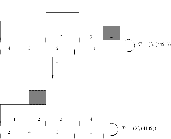
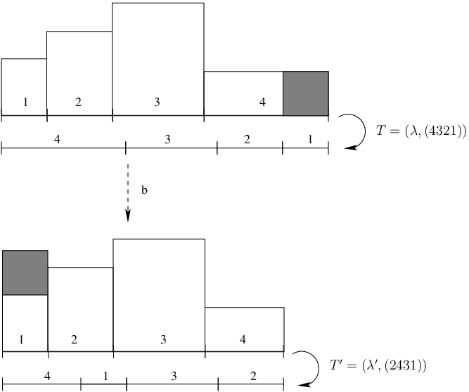
Since T(1)T^{(1)} is again an exchange of dd intervals, we can write T(1)=(λ(1),π(1))T^{(1)}=(\lambda^{(1)},\pi^{(1)}) (see Figure 1(c),1(d)), defining in this way a new lengths vector and a new permutation.

Refer to caption
(c) Case λd<λπ−1​(d)\lambda_{d}<\lambda_{\pi^{-1}(d)}
Refer to caption
(d) Case λd>λπ−1​(d)\lambda_{d}>\lambda_{\pi^{-1}({d})}
Figure 1: One step of Rauzy-Veech algorithm on T=(λ,(4321))T=(\lambda,(4321)).

One can explicitly write the expressions for two combinatorial operators aa and bb on 𝒮d\mathcal{S}_{d}, where 𝒮d\mathcal{S}_{d} is the space of permutations of dd elements, such that π(1)=a​π\pi^{(1)}=a\pi or b​πb\pi respectively. Explicitly:

a​π​(j)={π⁡(j)j≤π−1​(d);π⁡(d)j=π−1​(d)+1;π⁡(j−1)otherwise;a\pi(j)=\left\{\begin{array}[]{ll}\pi(j)&j\leq\pi^{-1}(d);\\ \pi(d)&j=\pi^{-1}(d)+1;\\ \pi(j-1)&\mathrm{otherwise};\\ \end{array}\right.
b​π​(j)={π⁡(j)j≤π⁡(d);π⁡(j)+1π⁡(d)<π⁡(j)<d;π⁡(d)+1π⁡(j)=d.b\pi(j)=\left\{\begin{array}[]{ll}\pi(j)&j\leq\pi(d);\\ \pi(j)+1&\pi(d)<\pi(j)<d;\\ \pi(d)+1&\pi(j)=d.\\ \end{array}\right.

Introduce the following matrices to describe the new lengths. Denote by Id the identity d×dd\times d matrix and by Ei,jE_{i,j} the matrix whose only non zero entry is (Ei,j)i​j=1(E_{i,j})_{ij}=1. Introduce the auxiliary permutation τs∈Sd\tau_{s}\in S^{d}, τs=(1  2​…​s​s+2​…​d​s+1)\tau_{s}=(1\,\,2\,\,\dots\,s\,\,s\!+\!2\,\,\,\dots\,\,d\,\,s\!+\!1) if 1≤s<d−11\leq s<d-1 and τd−1=id\tau_{d-1}=\mathrm{id}, which rotates cyclically all elements after the st​hs^{th}-one. Denote by P⁡(τs)P(\tau_{s}) the matrix associated to the permutation, i.e. P​(τs)i​j=δi​τs​(i)P(\tau_{s})_{ij}=\delta_{i\tau_{s}(i)}. The two Rauzy-Veech elementary matrices associated to (λ¯,π)(\underline{\lambda},\pi) are defined by

{A⁡(π,a)=(𝐼𝑑+Eπ−1​(d),d)⋅P⁡(τπ−1​(d));A⁡(π,b)=𝐼𝑑+Ed,π−1​(d).\left\{\begin{array}[]{rcl}A(\pi,a)&=&({\it Id}+E_{\pi^{-1}(d),d})\cdot P(\tau_{\pi^{-1}(d)});\\ A(\pi,b)&=&{\it Id}+E_{d,\pi^{-1}(d)}.\\ \end{array}\right. (10)

The induced IET T(1)T^{(1)} is then given by

(λ¯(1),π(1))≑{(A−1​(π,a)⋅λ¯,a⁡(π)),λd<λπ−1​(d);(A−1​(π,b)⋅λ¯,b⁡(π)),λd>λπ−1​(d).(\underline{\lambda}^{(1)},\pi^{(1)})\doteqdot\left\{\begin{array}[]{ll}\left(A^{-1}(\pi,\,a)\cdot\underline{\lambda},\,a(\pi)\right),&\lambda_{d}<\lambda_{\pi^{-1}({d})};\\ \left(A^{-1}(\pi,\,b)\cdot\underline{\lambda},\,b(\pi)\right),&\lambda_{d}>\lambda_{\pi^{-1}({d})}.\\ \end{array}\right. (11)

Remark that both A⁡(π,a)A(\pi,a) and A⁡(π,b)A(\pi,b) belong to S​L​(d,ℤ)SL(d,\mathbb{Z}) and have non-negative entries.

Define inductively T(r)=(λ¯(r),π(r))T^{(r)}=(\underline{\lambda}^{(r)},\pi^{(r)}) to be the induced map of T(r−1)T^{(r-1)} on I(r)I^{(r)}. It can be seen that the (IDOC) assures that the algorithm is well defined at each step, i.e. that λd(r−1)≠λ(π(r−1))−1​(d)(r−1)\lambda^{(r-1)}_{d}\neq\lambda^{(r-1)}_{(\pi^{(r-1)})^{-1}(d)} for any r∈ℕr\in\mathbb{N}.

Renormalized Rauzy-Veech map.

The Rauzy class of π\pi, denoted by ℛ⁡(π)⊂Sd\mathscr{R}(\pi)\subset S_{d}, is the set of all permutations obtained iterating the operators aa and bb starting from π\pi. Using the norm |λ¯|=∑i=1dλi|\underline{\lambda}|=\sum_{i=1}^{d}\lambda_{i}, assume that the initial lengths belong to the simplex Δd−1\Delta_{d-1} of vectors λ¯∈ℝ+d\underline{\lambda}\in\mathbb{R}^{d}_{+} such that |λ¯|=1|\underline{\lambda}|=1. Let us denote by Δ⁡(ℛ)=Δd−1×ℛ⁡(π)\Delta(\mathscr{R})=\Delta_{d-1}\times\mathscr{R}(\pi) the space of IETs on the unit interval corresponding to a given Rauzy class ℛ\mathscr{R}.

Consider the map on Δ⁡(ℛ)\Delta(\mathscr{R}) which associates to TT the induced IET after one step of the algorithm including the following renormalization:

ℛ⁡((λ¯(0),π(0)))≑(λ¯(1)|λ¯(1)|,π(1)).\mathcal{R}\left((\underline{\lambda}^{(0)},\pi^{(0)})\right)\doteqdot\left(\frac{\underline{\lambda}^{(1)}}{|\underline{\lambda}^{(1)}|},\pi^{(1)}\right).

Let us call it the Rauzy-Veech map. Veech proved that ℛ\mathscr{R} admits an invariant measure μ𝒱\mu_{\mathcal{V}}, absolutely continuous with respect to the Lebesgue measure, which is infinite. The main result proved by Veech in [Vee82] is that the map ℛ\mathcal{R} is conservative. As a consequence, he proves that given π∈𝒮d\pi\in\mathcal{S}_{d}, for a.e. λ¯∈Δd−1\underline{\lambda}\in\Delta_{d-1}, the IET T=(λ¯,π)T=(\underline{\lambda},\pi) is uniquely ergodic.

Zorich acceleration.

Take an IET TT and consider its Rauzy-Veech orbit {ℛn​T}n∈ℕ\{\mathcal{R}^{n}T\}_{n\in\mathbb{N}}. In a typical situation one can find an integer zo=zo​(T)>0z_{o}=z_{o}(T)>0 so that T,ℛ​T,…,ℛz0−1​(T)T,\mathcal{R}T,\dots,\mathcal{R}^{z_{0}-1}(T) all correspond to the same case (a)(a) or (b)(b) while ℛzo​(T)\mathcal{R}^{z_{o}}(T) corresponds to the other one. Grouping together these z0z_{0} steps of Rauzy induction, we get a new transformation 𝒵\mathcal{Z} on the space of IET, where the letter 𝒵\mathcal{Z} is chosen in honor of A. Zorich who introduced this map in [Zor96]. Zorich showed in [Zor96] that 𝒵\mathcal{Z} has an absolutely continuous finite invariant measure. We will denote the Zorich invariant measure by μ𝒵\mu_{\mathcal{Z}} .

2.1.2 Rauzy-Veech lengths cocycle.

As was explained above, to each TT one can associate an elementary matrix A⁡(T)A(T) in S​L​(d,ℤ)SL(d,\mathbb{Z}) defining A⁡(T)≑A⁡(π,a)A(T)\doteqdot A(\pi,a) or A⁡(T)≑A⁡(π,b)A(T)\doteqdot A(\pi,b) respectively. Let Ar=Ar​(T)≑A⁡(ℛr​T)A_{r}=A_{r}(T)\doteqdot A(\mathcal{R}^{r}T). Then for each rr we can associate to TT the product:

A(r)≑A1​…​Ar.A^{(r)}\doteqdot A_{1}\dots A_{r}.

We can easily see that the map A−1A^{-1}: Δ⁡(ℛ)→S​L​(d,ℤ)\Delta(\mathscr{R})\rightarrow SL(d,\mathbb{Z}) is a cocycle over ℛ\mathcal{R}, which we call the Rauzy-Veech lengths cocycle. Iterating the lengths relation in (11) we get the formula for the lengths vector of T(r)T^{(r)}:

λ¯(r)=(A(r))−1​λ¯.\underline{\lambda}^{(r)}=\left(A^{(r)}\right)^{-1}\underline{\lambda}. (12)

Let us also introduce the following notation useful to consider more generally products of Rauzy-Veech cocycle matrices from mm to nn, m<nm<n:

A(m,n)≑Am⋅Am+1⋅…⋅An−2⋅An−1.A^{(m,n)}\doteqdot A_{m}\cdot A_{m+1}\cdot\,\dots\,\cdot A_{n-2}\cdot A_{n-1}.

2.1.3 Hilbert metric and projective contractions.

Consider on the simplex Δd−1⊂ℝ+d\Delta_{d-1}\subset\mathbb{R}_{+}^{d} the Hilbert distance dHd_{H}, defined as follows.

dH​(λ,λ′)≑log⁡maxi=1,…,d⁡λiλi′mini=1,…,d⁡λiλi′.d_{H}(\lambda,\lambda^{\prime})\doteqdot\log\frac{\max_{i=1,\dots,d}\frac{\lambda_{i}}{\lambda^{\prime}_{i}}}{\min_{i=1,\dots,d}\frac{\lambda_{i}}{\lambda^{\prime}_{i}}}. (13)

We denote the diameter with respect to dHd_{H} of a projective subset Λ⊂Δd−1\Lambda\subset\Delta_{d-1} by

d​i​a​mH​(Λ)≑supλ,λ′∈ΛdH​(λ,λ′).diam_{H}(\Lambda)\doteqdot\sup_{\lambda,\lambda^{\prime}\in\Lambda}d_{H}(\lambda,\lambda^{\prime}). (14)

Remark that if its closure Λ¯⊂Δd−1\overline{\Lambda}\subset\Delta_{d-1}, then d​i​a​mH​(Λ)diam_{H}(\Lambda) is finite.

Let us write A≥0A\geq 0 if AA has non negative entries and A>0A>0 is AA has strictly positive entries. Recall that to each A∈S​L​(d,ℤ)A\in SL(d,\mathbb{Z}), A≥0A\geq 0, one can associate a projective transformation A~:Δd−1→Δd−1\widetilde{A}:\Delta_{d-1}\rightarrow\Delta_{d-1} given by

A~​λ=A​λ|A​λ|.\widetilde{A}\lambda=\frac{A\lambda}{|A\lambda|}.

When A≥0A\geq 0, dH​(A~​λ,A~​λ′)≤dH​(λ,λ′)d_{H}(\widetilde{A}\lambda,\widetilde{A}\lambda^{\prime})\leq d_{H}(\lambda,\lambda^{\prime}). Furthermore, if A>0A>0, then we get a contraction. More precisely, A>0A>0 is equivalent to the closure A~​(Δd−1)¯\overline{\widetilde{A}\left(\Delta_{d-1}\right)} being contained in Δd−1\Delta_{d-1}, hence defining

D⁡(A)≑d​i​a​mH​(A~​(Δd−1)¯),D(A)\doteqdot diam_{H}\left(\,\overline{\widetilde{A}\left({\Delta}_{d-1}\right)}\,\right), (15)

we have D⁡(A)<∞D(A)<\infty. Then

dH​(A~​λ,A~​λ′)≤(1−e−D⁡(A))​dH​(λ,λ′).d_{H}(\widetilde{A}\lambda,\widetilde{A}\lambda^{\prime})\leq(1-e^{-D(A)})d_{H}(\lambda,\lambda^{\prime}). (16)
Paths on Rauzy classes.

Rauzy classes can be visualized in terms of directed labeled graphs, the Rauzy graphs. Vertices are in one-to-one correspondence with permutations of ℛ⁡(π)\mathscr{R}(\pi); arrows connect permutations obtained one from the other by applying aa or bb and are labeled according to the type, aa or bb respectively. Each vertex is the starting point and the ending point of exactly two arrows, one of each type. We will denote by γi=γi​(π′,a)\gamma_{i}=\gamma_{i}(\pi^{\prime},a) (γi​(π′,b)\gamma_{i}(\pi^{\prime},b)) the arrow of type aa (type bb) coming out from the vertex π′\pi^{\prime}.

A path γ=(γ1,…,γr)\gamma=(\gamma_{1},\dots,\gamma_{r}) is a sequence of compatible arrows on the Rauzy graph, i.e. such that the starting vertex of γi+1\gamma_{i+1} is the ending vertex of γi\gamma_{i}, i=1,…,r−1i=1,\dots,r-1. Given a path γ\gamma, we can associate to it a matrix

A⁡(γ)≑A⁡(γ1)⋅…⋅A⁡(γr),A(\gamma)\doteqdot A(\gamma_{1})\cdot\,\dots\,\cdot A(\gamma_{r}),

where A⁡(γi)=A⁡(π′,a)A(\gamma_{i})={A(\pi^{\prime},a)} if γi=γi​(πi,a)\gamma_{i}=\gamma_{i}(\pi_{i},a) and A⁡(πi,b){A(\pi_{i},b)} if γi=γi​(πi,b)\gamma_{i}=\gamma_{i}(\pi_{i},b). Associate to γ\gamma also the subsimplex:

Δ(γ)≑{A⁡(γ)~λ¯|λ¯∈Δd−1}⊂Δd−1.\Delta(\gamma)\doteqdot\left\{\widetilde{A(\gamma)}\,\underline{\lambda}\,|\quad\underline{\lambda}\in\Delta_{d-1}\right\}\subset\Delta_{d-1}. (17)

Using the induction, one can easily verify the following.

Remark 1.

If T=(λ¯,π)T=(\underline{\lambda},\pi) and λ¯∈Δ⁡(γ)\underline{\lambda}\in\Delta(\gamma) where γ=(γ1,…,γr)\gamma=(\gamma_{1},\dots,\gamma_{r}) is a path starting at π\pi, γi=γi​(πi,ci)\gamma_{i}=\gamma_{i}(\pi_{i},c_{i}), ci∈{a,b}c_{i}\in\{a,b\}, the sequence of types and permutations obtained in the first rr steps of Rauzy-Veech induction is determined by γ\gamma, i.e. Ai​(T)=A⁡(γi)A_{i}(T)=A(\gamma_{i}) and π(i)=πi\pi^{(i)}=\pi_{i}.

2.1.4 The natural extension.

The natural extension ℛ^\hat{\mathcal{R}} of the map ℛ\mathcal{R} was introduced by Veech [Vee82] and admits a geometric interpretation in terms of the space of zippered rectangles. We use the simpler choice of coordinates for zippered rectangles, adopted by [Buf, MMY05, AGY].

Consider the following polyhedral cones Θπ⊂ℝd\Theta_{\pi}\subset\mathbb{R}^{d}, where π∈ℛ\pi\in\mathscr{R}.

Θπ≑{τ¯=(τ1,…,τd)∈ℝd|∑i=1kτi>0,∑i=1kτπ−1​i<0,k=1,…,d−1},\Theta_{\pi}\doteqdot\{\underline{\tau}=(\tau_{1},\dots,\tau_{d})\in\mathbb{R}^{d}|\quad\sum_{i=1}^{k}\tau_{i}>0,\,\sum_{i=1}^{k}\tau_{\pi^{-1}i}<0,\,k=1,\dots,d-1\},

which is non-empty since if τi≑π⁡(i)−i\tau_{i}\doteqdot\pi(i)-i, τ¯∈Θπ\underline{\tau}\in\Theta_{\pi}.

The real valued function A​r​e​a​(⋅)Area(\cdot) associates to (λ¯,π,τ¯)∈Δd−1×{π}×Θπ(\underline{\lambda},\pi,\underline{\tau})\in\Delta_{d-1}\times\{\pi\}\times\Theta_{\pi},

A​r​e​a​(λ¯,π,τ¯)≑∑k=1dλk​(∑i=1k−1τi−∑i=1π⁡(k)−1τπ−1​i).Area(\underline{\lambda},\pi,\underline{\tau})\doteqdot\sum_{k=1}^{d}\lambda_{k}\,\left(\sum_{i=1}^{k-1}\tau_{i}-\sum_{i=1}^{\pi(k)-1}\tau_{\pi^{-1}i}\right).

A​r​e​a​(⋅)Area(\cdot) has a geometric interpretation as the area of the zippered rectangle associated to the datas (λ¯,π,τ¯)(\underline{\lambda},\pi,\underline{\tau}) (see e.g. [MMY05]).

Consider the following space as domain of the natural extension.

Υ^ℛ(1)≑{(λ¯,π,τ¯)|(λ¯,π)∈Δ(ℛ),τ¯∈Θπ,Area((λ¯,π,τ¯))=1}.\hat{\Upsilon}^{(1)}_{\mathscr{R}}\doteqdot\{(\underline{\lambda},\pi,\underline{\tau})|\quad(\underline{\lambda},\pi)\in\Delta(\mathscr{R}),\,\underline{\tau}\in\Theta_{\pi},\,Area((\underline{\lambda},\pi,\underline{\tau}))=1\}.

The map ℛ^:Υ^ℛ(1)→Υ^ℛ(1)\hat{\mathcal{R}}:\hat{\Upsilon}^{(1)}_{\mathscr{R}}\rightarrow\hat{\Upsilon}^{(1)}_{\mathscr{R}} is defined as follows.22 2 More precisely ℛ^\hat{\mathcal{R}} is defined on triples (λ¯,π,τ¯)(\underline{\lambda},\pi,\underline{\tau}) such that (λ¯,π)(\underline{\lambda},\pi) belong to the domain of ℛ\mathcal{R}.

ℛ^​((,,,,,))=(ℛ⁡(λ¯,π),|λ¯(1)|​τ¯(1))=(λ¯(1)|λ¯(1)|,π(1),|λ¯(1)|​τ¯(1)),\hat{\mathcal{R}}\left((\underline{\lambda}^{(0)},\pi^{(0)},\underline{\tau}^{(0)})\right)=\left(\mathcal{R}(\underline{\lambda},\pi),|\underline{\lambda}^{(1)}|\underline{\tau}^{(1)}\right)=\left(\frac{\underline{\lambda}^{(1)}}{|\underline{\lambda}^{(1)}|},\pi^{(1)},|\underline{\lambda}^{(1)}|\underline{\tau}^{(1)}\right),

where (λ¯(1),π(1))(\underline{\lambda}^{(1)},\pi^{(1)}) is defined in (11) and, analogously,

τ¯(1)≑{A−1​(π,a)⋅τ¯,λd<λπ−1​(d),A−1​(π,b)⋅τ¯,λd>λπ−1​(d).\underline{\tau}^{(1)}\doteqdot\left\{\begin{array}[]{ll}A^{-1}(\pi,\,a)\cdot\underline{\tau},&\lambda_{d}<\lambda_{\pi^{-1}({d})},\\ A^{-1}(\pi,\,b)\cdot\underline{\tau},&\lambda_{d}>\lambda_{\pi^{-1}({d})}.\\ \end{array}\right.

The map ℛ^\hat{\mathcal{R}} preserves an invariant measure m^\hat{m} which is the restriction to Υ^ℛ(1)\hat{\Upsilon}^{(1)}_{\mathscr{R}} of the Lebesgue measure. Denote by pp the projection

p:Υ^ℛ(1)→Δ⁡(ℛ),p⁡(λ¯,π,τ¯)=(λ¯,π).p:\hat{\Upsilon}^{(1)}_{\mathscr{R}}\rightarrow\Delta(\mathscr{R}),\qquad p(\underline{\lambda},\pi,\underline{\tau})=(\underline{\lambda},\pi).

The measure p​m^p\hat{m} is absolutely continuous w.r.t. Lebesgue on Δ⁡(ℛ)\Delta(\mathscr{R}) and it is exactly the ℛ\mathcal{R}-invariant measure μ𝒱\mu_{\mathcal{V}} constructed by Veech.

If γ\gamma is a path on ℛ\mathscr{R}, starting at π\pi, denote by

Θ(γ)≑{A(γ)−1τ¯|τ¯∈Θπ}⊂ℝd.\Theta(\gamma)\doteqdot\left\{{A(\gamma)}^{-1}\,\underline{\tau}\,|\quad\underline{\tau}\in\Theta_{\pi}\right\}\subset\mathbb{R}^{d}.

If γ\gamma is an arrow starting at π\pi and ending at π′\pi^{\prime}, then ℛ^\hat{\mathcal{R}} maps

(Δ⁡(γ)×{π}×Θπ)∩Υ^ℛ(1)→ℛ^(Δd−1×{π′}×Θ⁡(γ))∩Υ^ℛ(1).\left(\Delta(\gamma)\times\{\pi\}\times\Theta_{\pi}\right)\cap\hat{\Upsilon}^{(1)}_{\mathscr{R}}\xrightarrow{\hat{\mathcal{R}}}\left(\Delta_{d-1}\times\{\pi^{\prime}\}\times\Theta(\gamma)\right)\cap\hat{\Upsilon}^{(1)}_{\mathscr{R}}.

As λ¯\underline{\lambda} determines the future induction steps (see Remark 1), similarly τ¯\underline{\tau} determines the past ones. More precisely, let (λ¯(−i),π(−i),τ¯(−i))≑ℛ^−i​(λ¯,π,τ¯)(\underline{\lambda}^{(-i)},\pi^{(-i)},\underline{\tau}^{(-i)})\doteqdot\hat{\mathcal{R}}^{-i}(\underline{\lambda},\pi,\underline{\tau}), for i∈ℕi\in\mathbb{N}.

Remark 2.

If π′\pi^{\prime} is the ending vertex of γ=(γ1,…,γr)\gamma=(\gamma_{1},\dots,\gamma_{r}) where γi=γi​(πi,ci)\gamma_{i}=\gamma_{i}(\pi_{i},c_{i}), ci∈{a,b}c_{i}\in\{a,b\}, and τ¯∈Θ⁡(γ)\underline{\tau}\in\Theta(\gamma), the sequence of types and permutations obtained in the past rr steps of ℛ^\hat{\mathcal{R}} is determined by γ\gamma, i.e. A⁡(λ(−i),π(−i))=A⁡(γr−i+1)A(\lambda^{(-i)},\pi^{(-i)})=A(\gamma_{r-i+1}) and π(−i)=πr−i+1\pi^{(-i)}=\pi_{r-i+1} for i=1,…,ri=1,\dots,r.

2.2 Towers construction and heights vectors.

The initial interval exchange TT can be seen as a suspension over each of the induced T(r)T^{(r)} obtained at the rt​hr^{th} step of Rauzy-Veech algorithm. In this subsection we define the towers which allow to retrieve TT from T(r)T^{(r)} and A(r)A^{(r)}.

Note that the entries of A(r)A^{(r)} have a dynamical meaning in terms of return times. Namely, denote Ij(r)I^{(r)}_{j}, 1≤j≤d1\leq j\leq d, the subintervals of T(r)T^{(r)}.

Remark 3.

The entry Ai​j(r)A^{(r)}_{ij} is equal to the number of visits of the orbit of any point x∈Ij(r)x\in I^{(r)}_{j} to the interval Ii(0)I^{(0)}_{i} of the original partition before its first return in I(r)I^{(r)}.

Therefore, the norm hj(r)h^{(r)}_{j} of the jt​hj^{th} column of A(r)A^{(r)}, i.e. hj(r)≑∑i=1dAi​j(r)h^{(r)}_{j}\doteqdot\sum_{i=1}^{d}A^{(r)}_{ij} gives the return time of any x∈Ij(r)x\in I^{(r)}_{j} to I(r)I^{(r)}.

The towers.

Define

Zj(r)≑⋃l=0hj(r)−1Tl​Ij(r).Z^{(r)}_{j}\doteqdot\bigcup_{l=0}^{h^{(r)}_{j}-1}T^{l}I^{(r)}_{j}. (18)

When TT is ergodic, ⋃j=1dZj(r)\bigcup_{j=1}^{d}Z^{(r)}_{j} is a non-trivial TT-invariant set, therefore the sets Zj(r)Z^{(r)}_{j}, 1≤j≤d1\leq j\leq d give a partition of the whole II. Each Zj(r)Z^{(r)}_{j} can be visualized as a tower over Ij(r)⊂I(r)I^{(r)}_{j}\subset I^{(r)}, of height hj(r)h^{(r)}_{j} (see Figure 2). A floor of the tower, denoted by Zj,l(r)Z^{(r)}_{j,l}, is defined by Zj,l(r)≑Tl​Ij(r)Z^{(r)}_{j,l}\doteqdot T^{l}I^{(r)}_{j} , l=0,…,hj(r)−1l=0,\dots,h^{(r)}_{j}-1. The original TT is an integral map over I(r)I^{(r)}; under the action of TT every floor Zj,l(r)Z^{(r)}_{j,l}, but the top one (l≠hj(r)l\neq h^{(r)}_{j}), moves one step up, while T⁡(Zj,hj(r)(r))=T(r)​(Ij(r))T\left(Z^{(r)}_{j,h^{(r)}_{j}}\right)=T^{(r)}\left(I^{(r)}_{j}\right).

Heights cocycle.

Let h¯(0)\underline{h}^{(0)} be the column vector e¯≑(1,…,1)T∈ℤd\underline{e}\doteqdot(1,\dots,1)^{T}\in\mathbb{Z}^{d} and h¯(n)\underline{h}^{(n)} the column vector whose components are the heights (h1(1),…,hd(1))T(h^{(1)}_{1},\dots,h^{(1)}_{d})^{T} of the towers after the first step of the Rauzy-Veech algorithm. If we write h¯(1)=R​h¯(0)\underline{h}^{(1)}=R\,\,\underline{h}^{(0)}, where R=R⁡(T)R=R(T) is a matrix in S​L​(d,ℤ)SL(d,\mathbb{Z}), it is easy to see that R⁡(T)=A​(π,a)TR(T)=A(\pi,a)^{T} or R⁡(T)=A​(π,b)TR(T)=A(\pi,b)^{T}, depending on whether the Rauzy step is of type (a)(a) or (b)(b).

Hence, comparing with (12), the cocycle that determines how the vectors of the heights transform is given by the inverse transpose of the Rauzy-Veech cocycle. More precisely, if h¯(r)\underline{h}^{(r)} is the vector of the heights after rr iterations of the algorithm, then

h¯(r)=(A(r))T​e¯;h¯(s+r)=A(r)​(ℛs​(T))T​h¯(s).\underline{h}^{(r)}=(A^{(r)})^{T}\,\,\underline{e};\qquad\underline{h}^{(s+r)}={A^{(r)}(\mathcal{R}^{s}(T))}^{T}\underline{h}^{(s)}\,. (19)

2.2.1 Recurrent structure of the towers.

Algorithm action on towers.

The Rauzy-Veech algorithm can be visualized as acting on the towers, in terms of stacking towers. One step corresponds to cutting the last tower before the permutation, i.e. Zd(r)Z^{(r)}_{d}, and stacking it over Zπ−1​d(r)Z^{(r)}_{\pi^{-1}d}. In the case aa, when λd(r)<λπ−1​d(r){\lambda}^{(r)}_{d}<\lambda^{(r)}_{\pi^{-1}d}, Zd(r)Z^{(r)}_{d} is completely cut and stacked above Zπ−1​d(r)Z^{(r)}_{\pi^{-1}d}, at its right end (see Figure 2(a)). In the case bb, λd(r)>λπ−1​d(r)\lambda^{(r)}_{d}>\lambda^{(r)}_{\pi^{-1}d}, only the right portion of Zd(r)Z^{(r)}_{d} of width λπ−1​d(r)\lambda^{(r)}_{\pi^{-1}d} is cut and stacked completely above Zπ−1​d(r)Z^{(r)}_{\pi^{-1}d} (see Figure 2(b)).

Refer to caption
(a) λd<λπ−1​(d)\lambda_{d}<\lambda_{\pi^{-1}(d)}
Refer to caption
(b) λd>λπ−1​(d)\lambda_{d}>\lambda_{\pi^{-1}(d)}
Figure 2: Stacking for T=(λ,(4321))T=(\lambda,(4321)).

It is clear from the stacking description of the algorithm that each tower Zj0(r)Z^{(r)}_{j_{0}} consists of pieces of towers Zj(s)Z^{(s)}_{j}.

Towers partitions.

Define the following system of measurable partitions ξs=ξs​(Zj0(r))\xi_{s}=\xi_{s}(Z^{(r)}_{j_{0}}) of the tower Zj0(r)Z^{(r)}_{j_{0}} in terms of the subtowers Zi(s)Z^{(s)}_{i}, 0≤s≤r0\leq s\leq r. The elements of the partition are complete blocks of floors of Zj0(r)Z^{(r)}_{j_{0}} which are all contained inside the same tower Zj(s)Z^{(s)}_{j}: namely, for each floor Zj0,l(r)Z^{(r)}_{j_{0},l} which is contained in I(s)I^{(s)}, construct an element Z∈ξsZ\in\xi_{s} in the following way. If Zj0,l(r)⊂Ij(s)Z^{(r)}_{j_{0},l}\subset I^{(s)}_{j},

Z≑⋃i=0hj(s)−1Ti​Zj0,l(r).Z\doteqdot\bigcup_{i=0}^{h^{(s)}_{j}-1}T^{i}Z^{(r)}_{j_{0},l}. (20)

The set of all such ZZ gives a partition ξs\xi_{s} of Zj0(r)Z^{(r)}_{j_{0}}. Clearly for each Z∈ξsZ\in\xi_{s} there is a unique jj such that Z⊂Zj(s)Z\subset Z^{(s)}_{j}. Partitions ξs′\xi_{s^{\prime}}, s′<ss^{\prime}<s, are refinements of ξs\xi_{s}.

The entries of A(m,n)A^{(m,n)} have the following meaning for the partition ξm​(Zj(n))\xi_{m}(Z^{(n)}_{j}). For m<nm<n, Ai​j(m,n)A^{(m,n)}_{ij} gives the number of visits of x∈Ij(n)x\in I^{(n)}_{j} to Ii(m)I^{(m)}_{i} under the action of T(m)T^{(m)} before the first return to I(m)I^{(m)}. Hence

Ai​j(m,n)=#{Z∈ξm(Zj(n))|Z⊂Zi(m)}.A^{(m,n)}_{ij}=\#\{Z\in\xi_{m}(Z^{(n)}_{j})|\quad Z\subset Z^{(m)}_{i}\}. (21)

2.3 Notation Summary.

For the convenience of the reader, we list in this section the notation relative to the induction algorithm for IETs introduced in the last paragraphs and used in the following ones.
ℛ\mathcal{R} Rauzy induction, ℛ\mathcal{R}: IETs →\rightarrow IETs; A−1A^{-1} Rauzy lengths cocycle, A−1A^{-1}: Δ⁡(ℛ)→S​L​(d,ℤ)\Delta(\mathscr{R})\rightarrow SL(d,\mathbb{Z}); AnA_{n} =A⁡(ℛn​T)=A(\mathcal{R}^{n}T) nt​hn^{th} elementary Rauzy matrix; A(n,m)A^{(n,m)} =An​…​Am−1=A_{n}\dots A_{m-1} product of Rauzy matrices; A(n)A^{(n)} =A(0,n)=A^{(0,n)};
I(n)I^{(n)} nt​hn^{th} inducing subinterval; T(n)T^{(n)} IET obtained as first return on I(n)I^{(n)}; Ij(n)I^{(n)}_{j} j=1,…,dj=1,\dots,d subintervals exchanged by T(n)T^{(n)}; λj(n)\lambda_{j}^{(n)} = |Ij(n)||I^{(n)}_{j}| length of Ij(n)I^{(n)}_{j}, w.r.t. the Lebesgue measure on II; λ¯(n)\underline{\lambda}^{(n)} = (λ1(n),…,λj(n),…,λd(n))(\lambda_{1}^{(n)},\dots,\lambda_{j}^{(n)},\dots,\lambda_{d}^{(n)}) lengths vector; λ(n){\lambda}^{(n)} = |λ¯(n)|=∑j=1dλj(n)|\underline{\lambda}^{(n)}|=\sum_{j=1}^{d}\lambda_{j}^{(n)} lenght |I(n)||I^{(n)}| of the nt​hn^{t}h inducing subinterval;
Ai​j(n,m)A^{(n,m)}_{ij} number of visits of x0∈Ij(m)x_{0}\in I^{(m)}_{j} to Ii(n)I^{(n)}_{i} before the first return to I(m)I^{(m)}; hj(n)h^{(n)}_{j} =∑iAi​j(n,m)=\sum_{i}A^{(n,m)}_{ij}, j=1,…,dj=1,\dots,d first return time of any x∈Ij(n)x\in I^{(n)}_{j} to I(n)I^{(n)}; Zj(n)Z^{(n)}_{j} =∪k=1hj(n)−1TkI(n)j=\cup_{k=1}^{h^{(n)}_{j}-1}T^{k}I^{(n)}_{j}, for j=1,…,dj=1,\dots,d towers representing TT over T(n)T^{(n)}; h(n){h}^{(n)} =maxj=1,…,d⁡hj(n)=\max_{j=1,\dots,d}h^{(n)}_{j} maximum of the towers heights; ξn\xi_{n} partition into floors of step nn, i.e Tk​(Ij(n))T^{k}(I^{(n)}_{j}), k≤hj(n)k\leq h^{(n)}_{j}, j=1,…,dj=1,\dots,d; ξn​(Z)\xi_{n}(Z) restriction of the partition ξn\xi_{n} to the set ZZ;
‖A‖\|A\| where A∈S​L​(d,ℤ)A\in SL(d,\mathbb{Z}), A≥0A\geq 0, is given by ‖A‖=∑i​jAi​j;\|A\|=\sum_{ij}A_{ij}; A>0A>0 (or OPENA≥0)A\geq 0) if A∈S​L​(d,ℤ)A\in SL(d,\mathbb{Z}) has positive (non-negative) entries; dHd_{H} Hilbert distance on Δd−1\Delta_{d-1}; d​i​a​mHdiam_{H} diameter w.r.t. the Hilbert distance; A~\widetilde{A} =A​λ¯/|A​λ¯|=A\underline{\lambda}/|A\underline{\lambda}| projective transformation associated to A≥0A\geq 0; D⁡(A)D(A) =d​i​a​mh​(A~​(Δd−1))=diam_{h}(\widetilde{A}(\Delta_{d-1})).

3 Growth of Birkhoff sums of derivatives.

Let us introduce two auxiliary functions uu, vv defined on I(0)I^{(0)}:

u⁡(x)≑1x;v⁡(x)≑11−x.u(x)\doteqdot\frac{1}{x};\qquad v(x)\doteqdot\frac{1}{1-x}.
Proposition 1.

Assume TT is uniquely ergodic. There exists a sequence αr\alpha_{r} such that αr→0\alpha_{r}\rightarrow 0 as r→∞r\rightarrow\infty and for all xx distinct from singularities of Sr​(f)S_{r}(f),

Sr​(f′)​(x)=(−C++αr+)​Sr​(u)​(x)+(C−+αr−)​Sr​(v)​(x),S_{r}(f^{\prime})(x)=(-C^{+}+\alpha_{r}^{+})S_{r}(u)(x)+(C^{-}+\alpha_{r}^{-})S_{r}(v)(x),

where |αr±|≤αr|\alpha_{r}^{\pm}|\leq\alpha_{r}.

Proof.

See Theorem 3.1 in [Koc03b]. The same proof applies also for uniquely ergodic IETs.∎

In Section 3.2 we prove estimates on the growth of the Birkhoff sums for uu and vv for a typical IET and then we use them in Section 3.3 to derive some information about the growth of Sr​(f′)S_{r}(f^{\prime}) and Sr​(f′′)S_{r}(f^{\prime\prime}). It is enough to get estimates from uu, since estimates from vv can be easily derived from the following observation. Let ℐ⁡(x)=1−x\mathcal{I}(x)=1-x, be the reflection on the interval I(0)I^{(0)}. Since v⁡(x)=u⁡(ℐ​x)v(x)=u(\mathcal{I}x), v⋅Tn=u⋅(ℐ⋅T⋅ℐ−1)n⋅ℐv\cdot T^{n}=u\cdot(\mathcal{I}\cdot T\cdot\mathcal{I}^{-1})^{n}\cdot\mathcal{I}. Let us denote by Tℐ≑ℐ⋅T⋅ℐ−1T^{\mathcal{I}}\doteqdot\mathcal{I}\cdot T\cdot\mathcal{I}^{-1}. Hence the Birkhoff sums for vv with respect to TT and the ones for uu with respect to TℐT^{\mathcal{I}} are related by

Sr​(v,T)​(x)=Sr​(u,Tℐ)​(1−x).S_{r}(v,T)(x)=S_{r}(u,T^{\mathcal{I}})(1-x). (22)

Remark that if T=((λ1,λ2,…,λn),π)T=((\lambda_{1},\lambda_{2},\dots,\lambda_{n}),\pi), then Tℐ=((λn,λn−1,…,λ1),πℐ)T^{\mathcal{I}}=((\lambda_{n},\lambda_{n-1},\dots,\lambda_{1}),\pi^{\mathcal{I}}) where πℐ≑(n​n−1​…​2 1)⋅π⋅(n​n−1​…​2 1)\pi^{\mathcal{I}}\doteqdot(n\,n\!-\!1\dots 2\,1)\cdot\pi\cdot(n\,n\!-\!1\dots 2\,1). Hence the map T↦TℐT\mapsto T^{\mathcal{I}} from Δd−1×ℛ⁡(π)→Δd−1×ℛ⁡(πℐ)\Delta_{d-1}\times\mathscr{R}(\pi)\rightarrow\Delta_{d-1}\times\mathscr{R}(\pi^{\mathcal{I}}) preserves the Lebesgue measure.

3.1 A diophantine-type condition for IETs.

In this section we define the set of full measure of IETs for which we prove Theorem 1. Proposition 2 shows that for typical TT one can find a subsequence {nl}l∈ℕ\{n_{l}\}_{l\in\mathbb{N}} of induction times such that the corresponding IETs {ℛnl​T}l∈ℕ\{\mathcal{R}^{n_{l}}T\}_{l\in\mathbb{N}} in the Rauzy orbit {ℛn​T}n∈ℕ\{\mathcal{R}^{n}T\}_{n\in\mathbb{N}} enjoy some good properties (listed in the Proposition 2 below), which we call balance; moreover it gives a control on their frequencies. In the next Sections we will use these balanced induction times in order to estimate the growth of Sr​(u)S_{r}(u).

Balanced times are related to occurrences of some positive matrices in the renormalization cocycle. Conditions on the frequencies of occurrence of such matrices play for interval exchanges a role analogous to diophantine conditions for rotations. Different type of estimates in this spirit appear in the works of [Ker85, MMY05, Buf, AGY]. The condition that we use is derived from [AGY].

3.1.1 Existence of balanced return times.

Proposition 2.

Let 1<τ<21<\tau<2. For each π\pi and for Lebesgue a.e. λ∈Δd−1\lambda\in\Delta_{d-1}, there exist a subsequence {nl}l∈ℕ\{n_{l}\}_{l\in\mathbb{N}} of induction times, ν>1\nu>1, κ>1\kappa>1, 0<D<∞0<D<\infty and l¯∈ℕ\overline{l}\in\mathbb{N}, such that the following properties hold for all l∈ℕl\in\mathbb{N}:

  1. 1.

    ( ν\nu -balance of lengths )

    1ν≤λi(nl)λj(nl)≤ν,∀ 1≤i,j≤d;\frac{1}{\nu}\leq\frac{\lambda_{i}^{(n_{l})}}{\lambda_{j}^{(n_{l})}}\leq\nu,\quad\forall\,1\leq i,\,j\leq d; (23)
  2. 2.

    (κ\kappa -balance of heights)

    1κ≤hi(nl)hj(nl)≤κ,∀ 1≤i,j≤d;\frac{1}{\kappa}\leq\frac{h_{i}^{(n_{l})}}{h_{j}^{(n_{l})}}\leq\kappa,\quad\forall\,1\leq i,\,j\leq d; (24)
  3. 3.

    (positivity)

    A(nl,nl+l¯)>0,andD⁡(A(nl,nl+l¯))≤D.A^{(n_{l\phantom{\overline{l}}},n_{l+\overline{l}})}>0,\quad\mathrm{and}\quad D({A^{(n_{l\phantom{\overline{l}}},n_{l+\overline{l}})}})\leq D. (25)
  4. 4.

    (integrability)

    liml→+∞‖A(nl,nl+1)‖lτ=0.\lim_{l\rightarrow+\infty}\frac{\|A^{(n_{l},n_{l+1})}\|}{l^{\tau}}=0. (26)

A return time which satisfies Properties 11 and 22 will be called balanced return time. A balanced return time is such that the lengths and the heights of the induction towers are approximately of the same size. Property 33 gives some uniform distribution of subintervals of time nl+l¯n_{l+\overline{l}} inside the subintervals of the previous balanced time nln_{l}. Property 44 is the diophantine condition which guarantees some control of the frequencies of occurrence of balanced times. It will be deduced from the power integrability of a certain induced cocycle, proved in [AGY].

We remark that (26) is analogous to the diophantine condition used for rotations in [SK92], i.e. kl=o⁡(lτ)k_{l}=o(l^{\tau}), where {kl}l∈ℕ\{k_{l}\}_{l\in\mathbb{N}} are the entries of the continued fraction and the exponent τ\tau satisfies the same assumption 1<τ<21<\tau<2.

Definition 1.

Let ℳ+=ℳ+​(Δd−1×ℛ⁡(π))\mathcal{M}^{+}=\mathcal{M}^{+}(\Delta_{d-1}\times\mathscr{R}(\pi)) be the set of IETs in Δd−1×ℛ⁡(π)\Delta_{d-1}\times\mathscr{R}(\pi) such that Proposition 2 hold and ℳ−=ℳ−​(Δd−1×ℛ⁡(π))\mathcal{M}^{-}=\mathcal{M}^{-}(\Delta_{d-1}\times\mathscr{R}(\pi)) be the set of T∈Δd−1×ℛ⁡(π)T\in\Delta_{d-1}\times\mathscr{R}(\pi) such that Tℐ∈ℳ+​(Δd−1×ℛ⁡(πℐ))T^{\mathcal{I}}\in\mathcal{M}^{+}(\Delta_{d-1}\times\mathscr{R}(\pi^{\mathcal{I}})). Denote ℳ=ℳ+∩ℳ−.\mathcal{M}=\mathcal{M}^{+}\cap\mathcal{M}^{-}.

The IETs in ℳ\mathcal{M} are the ones for which we prove mixing of the suspension flows having one asymmetric logarithmic singularity.

Remark 4.

The set ℳ\mathcal{M} has full measure. Indeed, ℳ+\mathcal{M}^{+} has full measure by Proposition 2 and also ℳ−\mathcal{M}^{-} has full measure since, as already remarked, T↦TℐT\mapsto T^{\mathcal{I}} preserves the Lebesgue measure.

Remark 5.

The IETs in ℳ\mathcal{M} are uniquely ergodic, as it follows from Property (25) in Proposition 2 with the help of techniques used by Veech in [Vee82, Vee81].

In the remaining part of this section we derive Proposition 2 from a result in [AGY] and then prove some simple corollaries, which will be used later.

3.1.2 Proof of Proposition 2.

If Y⊂Υ^ℛ(1)Y\subset\hat{\Upsilon}^{(1)}_{\mathscr{\mathcal{R}}}, let AYA_{Y} denote the induced cocycle of the Rauzy-Veech lengths cocycle associated to first returns to YY under ℛ^\hat{\mathcal{R}}, i.e. for (λ¯,π,τ¯)∈Y(\underline{\lambda},\pi,\underline{\tau})\in{Y},

AY(λ¯,π,τ¯)≑A(rY)((λ¯,π)),whererY≑min{r∈ℕ+|ℛ^r(λ¯,π,τ¯)∈Y}.A_{Y}(\underline{\lambda},\pi,\underline{\tau})\doteqdot A^{(r_{Y})}\left((\underline{\lambda},\pi)\right),\quad\mathrm{where}\quad r_{Y}\doteqdot\min\{r\in\mathbb{N}^{+}|\quad\hat{\mathcal{R}}^{r}(\underline{\lambda},\pi,\underline{\tau})\in Y\}.

The following result is proved in [AGY].

Theorem 2 (Avila, Gouëzel, Yoccoz).

For every δ>0\delta>0 there exists a finite union

Z^(1)≑(⋃i=1nΔ⁡(γsi)×{πi}×Θ⁡(γei))∩Υ^ℛ(1),\hat{Z}^{(1)}\doteqdot\left(\bigcup_{i=1}^{n}\Delta(\gamma_{s_{i}})\times\{\pi_{i}\}\times\Theta(\gamma_{e_{i}})\right)\cap\hat{\Upsilon}^{(1)}_{\mathscr{R}},

where πi\pi_{i} is both the initial permutation of the path γsi\gamma_{s_{i}} and the final one of the path γei\gamma_{e_{i}} and where A⁡(γsi)>0A(\gamma_{s_{i}})>0 and A⁡(γei)>0A(\gamma_{e_{i}})>0 for all i=1,…,ni=1,\dots,n, such that

∫Z^(1)‖AZ^(1)‖1−δ​𝑑m^<∞.\int_{\hat{Z}^{(1)}}\|A_{\hat{Z}^{(1)}}\|^{1-\delta}\mathrm{d}\hat{m}<\infty. (27)

Theorem 2 is a reformulation of Theorem 4.104.10 in [AGY]. The original statement claims the integrability of e(1−δ)​rZ^(1)e^{(1-\delta)r_{\hat{Z}^{(1)}}}, where rZ^(1)r_{\hat{Z}^{(1)}} is the first return time of (λ¯,π,τ¯)∈Z^(1)(\underline{\lambda},\pi,\underline{\tau})\in\hat{Z}^{(1)} under the Veech flow, which is given by

rZ^(1)​((,,,,,))≑−log⁡|AZ^(1)−1​λ¯|=log⁡|AZ^(1)​λ¯′|,r_{\hat{Z}^{(1)}}((\underline{\lambda},\pi,\underline{\tau}))\doteqdot-\log|A_{\hat{Z}^{(1)}}^{-1}\,\underline{\lambda}\,|=\log|A_{\hat{Z}^{(1)}}\,\underline{\lambda}^{\prime}\,|,

where (λ¯′,π′)=RrZ^(1)​(λ¯,π)(\underline{\lambda}^{\prime},\pi^{\prime})=R^{r_{\hat{Z}^{(1)}}}(\underline{\lambda},\pi). The second equality follows by taking norms of AZ^(1)​λ¯′=λ¯/|AZ^(1)−1​λ¯|A_{\hat{Z}^{(1)}}\,\underline{\lambda}^{\prime}=\underline{\lambda}/|A_{\hat{Z}^{(1)}}^{-1}\,\underline{\lambda}\,|. Since λ¯′\underline{\lambda}^{\prime} belong to the compact set ∪i=1nΔ(γsi)\cup_{i=1}^{n}\Delta(\gamma_{s_{i}}),

log⁡|AZ^(1)​λ¯′|≥log⁡(mini⁡λi′​‖AZ^(1)‖)≥c​o​n​s​t+log⁡‖AZ^(1)‖.\log|A_{\hat{Z}^{(1)}}\underline{\lambda}^{\prime}|\geq\log(\min_{i}\lambda^{\prime}_{i}\,\|A_{\hat{Z}^{(1)}}\|)\geq const+\log\|A_{\hat{Z}^{(1)}}\|.

Hence (27) follows from the integrability of e(1−δ)​rZ^(1)e^{(1-\delta)r_{\hat{Z}^{(1)}}}. Positivity of A⁡(γsi)A(\gamma_{s_{i}}) and A⁡(γei)A(\gamma_{e_{i}}) is clear from the proof of Thm. 4.10, in which γsi\gamma_{s_{i}} and γei\gamma_{e_{i}} are chosen minimal and 2​d−32d-3 complete and hence positive by Lemma 3.33.3.

Proof of Proposition 2.

Given 1<τ<21<\tau<2, let δ≑1−τ−1>0\delta\doteqdot 1-\tau^{-1}>0. Let Z^(1)\hat{Z}^{(1)} be the corresponding set given by Theorem 2. Let l¯\overline{l} be the maximum length of the paths γsi\gamma_{s_{i}} and γei\gamma_{e_{i}} for i=1,…,ni=1,\dots,n.

Given (λ¯,π)(\underline{\lambda},\pi), choose any τ¯∈Θπ\underline{\tau}\in\Theta_{\pi}. Let {nl}l∈ℕ\{n_{l}\}_{l}\in\mathbb{N} be the subsequence of visits of the ℛ^\hat{\mathcal{R}} orbit of (λ¯,π,τ¯)(\underline{\lambda},\pi,\underline{\tau}) to Z^(1)\hat{Z}^{(1)} given by

n0\displaystyle n_{0} ≑\displaystyle\doteqdot min{n∈ℕ+|n≥l¯,ℛ^n(λ¯,π,τ¯)∈Z^(1)};\displaystyle\min\{n\in\mathbb{N}^{+}|\,n\geq\overline{l},\,\hat{\mathcal{R}}^{n}(\underline{\lambda},\pi,\underline{\tau})\in\hat{Z}^{(1)}\}; (28)
nl+1\displaystyle n_{l+1} ≑\displaystyle\doteqdot min{n∈ℕ+|n>nl,ℛ^n(λ¯,π,τ¯)∈Z^(1)};l∈ℕ+.\displaystyle\min\{n\in\mathbb{N}^{+}|\,n>n_{l},\,\hat{\mathcal{R}}^{n}(\underline{\lambda},\pi,\underline{\tau})\in\hat{Z}^{(1)}\};\qquad l\in\mathbb{N^{+}}. (29)

Notice that (28) is independent on τ¯\underline{\tau}, since as soon as nn is bigger than the maximum length l¯\overline{l} of the paths γei\gamma_{e_{i}}, visits to Z^(1)\hat{Z}^{(1)} are determined by λ¯\underline{\lambda} only (see Remark 1 and 2). Let us show that Properties 11, 22 (balance) and 33 (positivity) of Proposition 2 automatically hold for (λ¯,π)(\underline{\lambda},\pi) and the sequence {nl}l∈ℕ\{n_{l}\}_{l\in\mathbb{N}}.

Since by definition ℛ^nl​(λ¯,π,τ¯)∈Δ⁡(γsj)×{πj}×Θ⁡(γsj)\hat{\mathcal{R}}^{n_{l}}(\underline{\lambda},\pi,\underline{\tau})\in\Delta(\gamma_{s_{j}})\times\{\pi_{j}\}\times\Theta({\gamma_{s_{j}}}) for some jj, in particular λ(nl)/|λ(nl)|∈Δ⁡(γsj)\lambda^{(n_{l})}/|\lambda^{(n_{l})}|\in\Delta(\gamma_{s_{j}}). By positivity of the A⁡(γsi)>0A(\gamma_{s_{i}})>0, the union ∪iΔ(γsi)\cup_{i}\Delta(\gamma_{s_{i}}) is compact and hence (see subsection 2.1.3) contained in a ball for the Hilbert metric dHd_{H}, centered at (1/d,…,1/d)(1/d,\dots,1/d), of some radius rs>0r_{s}>0. Hence,

dH​(λ¯(nl)|λ¯(nl)|,(1d,…,1d))≤rsor​equivalentlymaxi⁡λi(nl)mini⁡λi(nl)≤ers,d_{H}\left(\frac{\underline{\lambda}^{(n_{l})}}{|\underline{\lambda}^{(n_{l})}|},\left(\frac{1}{d},\dots,\frac{1}{d}\right)\right)\leq r_{s}\quad\mathrm{or}\,\mathrm{equivalently}\quad\frac{\max_{i}\lambda^{(n_{l})}_{i}}{\min_{i}\lambda^{(n_{l})}_{i}}\leq e^{r_{s}},

which, setting ν≑ers>1\nu\doteqdot e^{r_{s}}>1, is ν\nu-balance of lengths.

Similarly, from τ¯(nl)∈Θ⁡(γej)\underline{\tau}^{(n_{l})}\in\Theta({\gamma_{e_{j}}}) we get by Remark 2 that λ¯(nl)=A​(γej)−1​λ¯(nl−L)\underline{\lambda}^{(n_{l})}=A(\gamma_{e_{j}})^{-1}\underline{\lambda}^{(n_{l}-L)}, where LL is length of γej\gamma_{e_{j}}. Since the heights transform according to (19), h¯(nl)=A​(γej)T​h¯(nl−L)\underline{h}^{(n_{l})}=A(\gamma_{e_{j}})^{T}\underline{h}^{(n_{l}-L)}. Arguing as above, by compactness, the union ∪iA​(γei)T~Δd−1\cup_{i}\widetilde{A(\gamma_{e_{i}})^{T}}\Delta_{d-1} is contained in a ball centered at (1/d,…,1/d)(1/d,\dots,1/d) of some radius re>0r_{e}>0 and this gives κ≑ere\kappa\doteqdot e^{r_{e}} balance of the heights.

For Property 33, since l¯\overline{l} is the maximum lengths of the paths γsi\gamma_{s_{i}} and nl+l¯≥nl+l¯n_{l+\overline{l}}\geq n_{l}+\overline{l}, by Remark 1 we have A(nl,nl+l¯)=A⁡(γsj)​AA^{(n_{l},n_{l+\overline{l}})}=A(\gamma_{s_{j}})A for some A≥0A\geq 0. Hence A(nl,nl+l¯)>0A^{(n_{l},n_{l+\overline{l}})}>0 and D⁡(A(nl,nl+l¯))≤D⁡(A⁡(γsj))≤2​rsD(A^{(n_{l},n_{l+\overline{l}})})\leq D\left(A(\gamma_{s_{j}})\right)\leq 2r_{s}.

Let us show first that Property 44 holds for typical (λ¯,π,τ¯)∈Z^(1)(\underline{\lambda},\pi,\underline{\tau})\in\hat{Z}^{(1)}. Remark that A(nl,nl+1)​(λ¯,π,τ¯)=AZ^(1)​(R^nl​(λ¯,π,τ¯))A^{(n_{l},n_{l+1})}(\underline{\lambda},\pi,\underline{\tau})=A_{\hat{Z}^{(1)}}(\hat{R}^{n_{l}}(\underline{\lambda},\pi,\underline{\tau})). For each ϵk≑1/k\epsilon_{k}\doteqdot 1/k, by ℛ^\hat{\mathcal{R}} invariance of m^\hat{m},

m^{(λ¯,π,τ¯)∈R^nl|∥A(nl,nl+1)(λ¯,π,τ¯)∥≥ϵklτ}==m^{(λ¯,π,τ¯)∈R^nl|∥AZ^(1)(λ¯,π,τ¯)∥τ−1ϵk−τ−1≥l}.\begin{split}\hat{m}\{(\underline{\lambda},\pi,\underline{\tau})\in\hat{R}^{n_{l}}|&\,\quad\|A^{(n_{l},n_{l+1})}(\underline{\lambda},\pi,\underline{\tau})\|\geq\epsilon_{k}l^{\tau}\}=\\ &=\hat{m}\{(\underline{\lambda},\pi,\underline{\tau})\in\hat{R}^{n_{l}}|\quad\|A_{\hat{Z}^{(1)}}(\underline{\lambda},\pi,\underline{\tau})\|^{\tau^{-1}}\epsilon_{k}^{-\tau^{-1}}\geq l\}.\end{split}

Since we chose τ−1=1−δ\tau^{-1}=1-\delta, the integrability condition (27) implies that ∑lm^{∥AZ^(1)∥τ−1ϵk−τ−1≥l}<∞\sum_{l}\hat{m}\{\|A_{\hat{Z}^{(1)}}\|^{\tau^{-1}}\epsilon_{k}^{-\tau^{-1}}\geq l\}<\infty for each ϵk\epsilon_{k}. Hence, it follows by Borel-Cantelli that there exists a subset Z^′⊂Z^(1)\hat{Z}^{\prime}\subset\hat{Z}^{(1)} with m^​(Z^′)=m^​(Z^(1))\hat{m}(\hat{Z}^{\prime})=\hat{m}(\hat{Z}^{(1)}) such that for (λ¯,π,τ¯)∈Z^′(\underline{\lambda},\pi,\underline{\tau})\in\hat{Z}^{\prime} the sequence nln_{l} satisfies (26).

Consider the projection p​Z^′⊂Δ⁡(ℛ)p\hat{Z}^{\prime}\subset\Delta(\mathscr{R}). By indipendence of the definition of {nl}\{n_{l}\} on τ\tau , for each (λ¯,π)∈p​Z^′(\underline{\lambda},\pi)\in p\hat{Z}^{\prime} we have (26). Moreover, p​Z^′p\hat{Z}^{\prime} has p​m^p\hat{m} full measure in pZ^(1)=∪iΔ(γsi)×{πi}p\hat{Z}^{(1)}=\cup_{i}\Delta(\gamma_{s_{i}})\times\{\pi_{i}\} and in particular positive p​m^=μ𝒱p\hat{m}=\mu_{\mathcal{V}} measure and hence also μZ\mu_{Z} positive measure.

To conclude, let ℳ+\mathcal{M}^{+} be the set of T∈Δ⁡(ℛ)T\in\Delta(\mathscr{R}) such that there exists n¯\overline{n}, for which Rn¯​T∈p​Z^′R^{\overline{n}}T\in p\hat{Z}^{\prime}. Clearly if T∈ℳ+T\in\mathcal{M}^{+}, all the Properties are satisfied by the sequence nl≑n~l+n¯n_{l}\doteqdot\widetilde{n}_{l}+\overline{n}, where n~l\widetilde{n}_{l} is the sequence associated to ℛn¯​T\mathcal{R}^{\overline{n}}T. To see that ℳ+\mathcal{M}^{+} has full measure, it is enough to use ergodicity of 𝒵\mathcal{Z} and the fact that μ𝒵​(p​Z^′)>0\mu_{\mathcal{Z}}(p\hat{Z}^{\prime})>0, remarking that 𝒵\mathcal{Z} orbits are subsets of ℛ\mathcal{R} orbits. The formulation in Proposition 2 follows by absolute continuity of μ𝒵\mu_{\mathcal{Z}} w.r.t. Lebesgue.

∎

3.1.3 Some consequences of balance.

We will also frequently use the following simple lemmas. Recall that A>0A>0 means that AA has strictly positive entries.

Lemma 2.

Let Ai>0A_{i}>0, Ai∈S​L​(d,ℤ)A_{i}\in SL(d,\mathbb{Z}) for i=0,…,ni=0,\dots,n. If λ¯=A0⋅λ¯′\underline{\lambda}=A_{0}\cdot\underline{\lambda}^{\prime}, then ∑jλj>d​∑jλj′\sum_{j}\lambda_{j}>d\sum_{j}\lambda_{j}^{\prime}.

If h¯=A0⋅h¯′\underline{h}=A_{0}\cdot\underline{h}^{\prime}, then minj⁡hj>d​minj​hj′\min_{j}h_{j}>d\min_{j}h_{j}^{\prime}. In particular if h¯=A1⋯Ane¯\underline{h}=A_{1}\cdots A_{n}\,\underline{e}, then minj⁡hj≥dn\min_{j}{h_{j}}\geq d^{n}.

Proof.

All the properties follow easily from Ai​j≥1A_{ij}\geq 1. ∎

Recall that we defined λ(nl)≑∑jλj(nl)\lambda^{(n_{l})}\doteqdot\sum_{j}\lambda^{(n_{l})}_{j} and h(nl)≑maxj⁡hj(nl)h^{(n_{l})}\doteqdot\max_{j}h^{(n_{l})}_{j}.

Corollary 1.

For each L∈ℕL\in\mathbb{N}, log⁡(h(nL​l¯))≥L​log⁡d\log(h^{(n_{L\overline{l}})})\geq{L}\log d. In particular,

liml→+∞1log⁡h(nl)=0.\lim_{l\rightarrow+\infty}\frac{1}{\log h^{(n_{l})}}=0. (30)
Proof.

For the first property, apply Lemma 2 to h(nL​l¯)=A(nL​l¯)T​e¯h^{(n_{L\overline{l}})}={A^{(n_{L\overline{l}})}}^{T}\underline{e} and remark that A(nL​l¯)T{A^{(n_{L\overline{l}})}}^{T} is the product of at least LL positive matrices by Property 3 (see (25)) of the sequence {nl}l∈ℕ\{n_{l}\}_{l\in\mathbb{N}}. It follows that log⁡h(nl)≥log⁡d⁡[l/l¯]\log h^{(n_{l})}\geq\log d[{l}/{\overline{l}}] and hence we get (30). ∎

Recall that we defined λ(nl)≑∑jλj(nl)\lambda^{(n_{l})}\doteqdot\sum_{j}\lambda^{(n_{l})}_{j} and h(nl)≑maxj⁡hj(nl)h^{(n_{l})}\doteqdot\max_{j}h^{(n_{l})}_{j}.

Lemma 3.

If nln_{l} has ν\nu-balanced lengths (23) and κ\kappa-balanced heights (24), then for each j=0,…,dj=0,\dots,d,

1κ​λ(nl)\displaystyle\frac{1}{\kappa\lambda^{(n_{l})}} ≤\displaystyle\leq hj(nl)≤κλ(nl);\displaystyle h^{(n_{l})}_{j}\leq\frac{\kappa}{\lambda^{(n_{l})}}; (31)
1d​κ​ν​h(nl)\displaystyle\frac{1}{d\kappa\nu h^{(n_{l})}} ≤\displaystyle\leq λj(nl)≤κh(nl).\displaystyle\lambda^{(n_{l})}_{j}\leq\frac{\kappa}{h^{(n_{l})}}. (32)

Hence, if nln_{l} is a balanced time, λ(nl)≈1/h(nl)\lambda^{(n_{l})}\approx 1/h^{(n_{l})} up to constants.

Proof.

Since by Kac lemma ∑ihi(nl)​λi(nl)=1\sum_{i}h^{(n_{l})}_{i}\lambda^{(n_{l})}_{i}=1, remark that mini⁡hi(nl)​λ(nl)≤1\min_{i}h^{(n_{l})}_{i}\lambda^{(n_{l})}\leq 1 and maxi⁡hi(nl)​λ(nl)≥1\max_{i}h^{(n_{l})}_{i}\lambda^{(n_{l})}\geq 1. Together with heights balance (24), this gives

1κ​λ(nl)≤1κ​maxi​hi(nl)≤hj(nl)≤κ​mini​hi(nl)≤κλ(nl).\frac{1}{\kappa\lambda^{(n_{l})}}\leq\frac{1}{\kappa}\max_{i}h^{(n_{l})}_{i}\leq h^{(n_{l})}_{j}\leq{\kappa}\min_{i}h^{(n_{l})}_{i}\leq\frac{\kappa}{\lambda^{(n_{l})}}.

To show (32), let ii be such that hi(nl)​λi(nl)=maxj⁡hj(nl)​λj(nl)≥1/dh^{(n_{l})}_{i}\lambda^{(n_{l})}_{i}=\max_{j}h^{(n_{l})}_{j}\lambda^{(n_{l})}_{j}\geq 1/d. Also, for each jj, hj(nl)​λj(nl)<1h^{(n_{l})}_{j}\lambda^{(n_{l})}_{j}<1. Using also lengths balance (23),

1κ​ν​d​h(nl)≤1ν​d​hi(nl)≤λi(nl)ν≤λj(nl)≤1hj(nl)≤κh(nl).\frac{1}{\kappa\nu dh^{(n_{l})}_{\phantom{j}}}\leq\frac{1}{\nu dh^{(n_{l})}_{i}}\leq\frac{\lambda^{(n_{l})}_{i}}{\nu}\leq\lambda^{(n_{l})}_{j}\leq\frac{1}{h^{(n_{l})}_{j}}\leq\frac{\kappa}{h^{(n_{l})}_{\phantom{j}}}.

∎

Lemma 4.

For each fixed L∈ℕL\in\mathbb{N},

liml→+∞log⁡‖A(nl,nl+L)‖log⁡h(nl)=liml→+∞log⁡‖A(nl−L,nl)‖log⁡h(nl)=0.\lim_{l\rightarrow+\infty}\frac{\log\|A^{(n_{l},n_{l+L})}\|}{\log h^{(n_{l})}}=\lim_{l\rightarrow+\infty}\frac{\log\|A^{(n_{l-L},n_{l})}\|}{\log h^{(n_{l})}}=0. (33)
Proof.

By Corollary 1, log⁡h(nl)≥[l/l¯]​log⁡d\log h^{(n_{l})}\geq{[l/\overline{l}]}\log d, where [⋅][\cdot] denotes the integer part. Hence

liml→+∞log⁡‖A(nl,nl+L)‖log⁡h(nl)≤liml→+∞∑i=ll+L−1log⁡‖A(ni,ni+1)‖(l/l¯−1)​log⁡d.\lim_{l\rightarrow+\infty}\frac{\log\|A^{(n_{l},n_{l+L})}\|}{\log h^{(n_{l})}}\leq\lim_{l\rightarrow+\infty}\frac{\sum_{i=l}^{l+L-1}\log\left\|A^{(n_{i},n_{i+1})}\right\|}{(l/\overline{l}-1)\log d}. (34)

Using the property (26), each of the LL terms in the sum in the RHS can be bounded for l≫1l\gg 1 by τ​log⁡i≤τ​log⁡(l+L−1)\tau\log i\leq\tau\log(l+L-1) and hence the first limit is zero. The second one is analogous. ∎

3.2 Growth of Birkhoff sums of uu.

Assume in this section that the roof function is u⁡(x)=1/xu(x)=1/x.

3.2.1 Growth of Birkhoff sums along a balanced tower.

In order to understand the asymptotic growth of Sr​(u)​(x)S_{r}(u)(x), we first consider Sr​(u)​(x)S_{r}(u)(x) when x∈Ij(n)x\in I^{(n)}_{j} is a point in the base of the tower Zj(n)Z^{(n)}_{j}, r=hj(n)r=h^{(n)}_{j} is exactly the height of the same tower and nn is one of the balanced return times constructed in Section 2. This preliminary estimate is used in Section 3.2.2 as a building block to get an estimate for any rr and most of the other points xx.

Proposition 3.

Assume T∈ℳ+T\in\mathcal{M}^{+}. Let nl0n_{l_{0}} be a balanced return time given by Proposition 2. Let x0∈Ij0(nl0)x_{0}\in I^{(n_{l_{0}})}_{j_{0}} be a point belonging to the base of the tower Zj0(nl0)Z^{(n_{l_{0}})}_{j_{0}} and let r0=hj0(nl0)r_{0}=h^{(n_{l_{0}})}_{j_{0}} be the corresponding tower height. Given ε>0\varepsilon>0, there exists l⁡(ε)l(\varepsilon) such that for l0≥l⁡(ε)l_{0}\geq l(\varepsilon),

(1−ε)​hj0(nl0)​ln⁡(h(nl0))≤Sr0​(u)​(x0)−1x0≤(1+ε)​hj0(nl0)​ln⁡(h(nl0)).(1-\varepsilon)h^{(n_{l_{0}})}_{j_{0}}\ln\left(h^{(n_{l_{0}})}\right)\leq S_{{r_{0}}}(u)(x_{0})-\frac{1}{x_{0}}\leq(1+\varepsilon)h^{(n_{l_{0}})}_{j_{0}}\ln\left(h^{(n_{l_{0}})}\right). (35)

A Birkhoff sum of the form Sr0​(u)​(x0)S_{{r_{0}}}(u)(x_{0}) where x0x_{0} and r0r_{0} satisfy the hypotheses of Proposition 3 will be referred as Birkhoff sum along a tower. The proposition shows that each sum along a tower gives a contribution of order r0​log⁡(r0)r_{0}\log(r_{0}), plus the contribution of the closest point to the singularity, x0x_{0}, which could be arbitrary large and will be estimated separately when using this sums as building blocks in Section 3.2.2.

Proof of Proposition 3.

Consider the inducing intervals I(nl)=[0,λ(nl)]I^{(n_{l})}=[0,\lambda^{(n_{l})}] where {nl}l∈ℕ\{n_{l}\}_{l\in\mathbb{N}} is the sequence of balanced induction times constructed in Section 3.1. Given any ϵ>0\epsilon>0, let DD and l¯\overline{l} be given by Proposition 2. Choose L1∈ℕL_{1}\in\mathbb{N} such that

(1−e−D)L1−1​D<ϵ.(1-e^{-D})^{L_{1}-1}D<\epsilon. (36)

We remark that d​i​a​m​(A(nl¯)~​Δd−1)<∞diam(\widetilde{A^{(n_{\overline{l}})}}\Delta_{d-1})<\infty by (25). Choose also L2∈ℕL_{2}\in\mathbb{N} such that 1/dL2<ϵ1/d^{L_{2}}<\epsilon. Assume l0≥l¯​(1+L1+L2)l_{0}\geq\overline{l}(1+L_{1}+L_{2}). For convenience, introduce the notation:

l−1≑l0−L1​l¯;l−2≑l−1−L2​l¯=l0−(L1+L2)​l¯;{l_{-1}}\doteqdot{l_{0}-L_{1}\overline{l}};\qquad{l_{-2}}\doteqdot{l_{-1}-L_{2}\overline{l}}={l_{0}-(L_{1}+L_{2})\overline{l}}; (37)

The past induction times nl−1n_{l_{-1}} and nl−2n_{l_{-2}} will play the following role in the proof: nl−1n_{l_{-1}} is such that the elements of the orbit {Tr​(x0)}0≤r<r0\{T^{r}(x_{0})\}_{0\leq r<r_{0}} are uniformly distributed inside the elements of the partition ξnl−1\xi_{n_{l_{-1}}}; nl−2n_{l_{-2}} is such that the main contribution to Sr0​(u)​(x0)S_{{r_{0}}}(u)(x_{0}) comes from visits to (λ(nl−2),1](\lambda^{(n_{l_{-2}})},1].

Denote the points along the TT-orbit of x0x_{0} by xi=Ti​(x0)x_{i}=T^{i}(x_{0}), 0≤i<r00\leq i<r_{0}. Since the original interval can be partitioned as

I(0)=I(nl0)∪I(nl−2)\I(nl0)∪(λ(nl−2),1],I^{(0)}=I^{(n_{l_{0}})}\cup I^{(n_{l_{-2}})}\backslash I^{(n_{l_{0}})}\cup(\lambda^{(n_{l_{-2}})},1],

and xi∉I(nl0)x_{i}\notin I^{(n_{l_{0}})}, for 1≤i<r01\leq i<r_{0} because r0r_{0} is by definition the first return time of x0x_{0} to I(nl0)I^{(n_{l_{0}})}, the Birkhoff sums can be decomposed as follows:

Sr0​(u)​(x0)=∑i=0r0−11xi=1x0+∑xi∈I(nl−2)\I(nl0)1xi+∑xi∈(λ(nl−2),1]1xi.S_{{r_{0}}}(u)(x_{0})=\sum_{i=0}^{r_{0}-1}\frac{1}{x_{i}}=\frac{1}{x_{0}}+\sum_{x_{i}\in I^{(n_{l_{-2}})}\backslash I^{(n_{l_{0}})}}\frac{1}{x_{i}}+\sum_{x_{i}\in(\lambda^{(n_{l_{-2}})},1]}\frac{1}{x_{i}}. (38)

We will refer to the first term in the RHS of (38) as singular error, to the sum which appears as a second term as gap error, while the sum which appears as a last term determines the main contribution.

Uniform ergodic convergence.

The following Lemma gives an uniform bound for the equidistribution of the orbits of points x∈I(nl0)x\in I^{(n_{l_{0}})} inside the elements of the past partition ξnl−1\xi_{n_{l_{-1}}}. Recall that Ai​j(nl−1,nl0)A^{(n_{l_{-1}},n_{l_{0}})}_{ij} gives the number of visits of x∈Ij(nl0)x\in I^{(n_{l_{0}})}_{j} to Ii(nl−1)I^{(n_{l_{-1}})}_{i} before the time hj(nl0)h^{(n_{l_{0}})}_{j} of first return to I(nl0)I^{(n_{l_{0}})}.

Lemma 5 (Uniform distribution).

For each 1≤i,j≤d1\leq i,\,j\leq d,

e−2​ϵ​λi(nl−1)≤Ai​j(nl−1,nl0)hj(nl0)≤e2​ϵ​λi(nl−1).e^{-2\epsilon}\lambda^{(n_{l_{-1}})}_{i}\leq\frac{A^{(n_{l_{-1}},n_{l_{0}})}_{ij}}{h^{(n_{l_{0}})}_{j}}\leq e^{2\epsilon}\lambda^{(n_{l_{-1}})}_{i}. (39)
Proof.

Consider the sets A(nl−1,n)~​Δd−1⊂Δd−1\widetilde{A^{(n_{l_{-1}},n)}}\Delta_{d-1}\subset\Delta_{d-1}, for n>nl−1n>n_{l_{-1}}, which form a nested sequence of compact sets. By the transformation formula (12) for lengths vectors λ¯(nl−1)=A(nl−1,n)​λ¯(n)\underline{\lambda}^{(n_{l_{-1}})}=A^{(n_{l_{-1}},n)}\underline{\lambda}^{(n)}, the renormalized vector

λ¯(nl−1)λ(nl−1)∈⋂n>nl−1A(nl−1,n)~​Δd−1.\frac{\underline{\lambda}^{(n_{l_{-1}})}}{\lambda^{(n_{l_{-1}})}}\in\bigcap_{n>n_{l_{-1}}}\widetilde{A^{(n_{l_{-1}},n)}}\Delta_{d-1}.

When n=nl0n=n_{l_{0}}, since l0=l−1+L1​l¯l_{0}=l_{-1}+L_{1}\overline{l}, applying L1L_{1} times Property 3 (positivity) in Proposition 2 through the contraction property (16), we get

d​i​a​mH​(A(nl−1,nl0)~​Δd−1)≤(1−e−D)L1−1​D≤ϵ,diam_{H}(\widetilde{A^{(n_{l_{-1}},n_{l_{0}})}}\Delta_{d-1})\leq(1-e^{-D})^{L_{1}-1}D\leq\epsilon, (40)

where the last inequality follows by the choice (36) of L1L_{1}.

Denote by e¯j\underline{e}_{j} the unit vector (e¯j)i=δi​j(\underline{e}_{j})_{i}=\delta_{ij} (δ\delta is here the Kronecker symbol). Since both the vectors A(nl−1,nl0)~​e¯j\widetilde{A^{(n_{l_{-1}},n_{l_{0}})}}\underline{e}_{j} and λ¯(nl−1)λ(nl−1)\frac{\underline{\lambda}^{(n_{l_{-1}})}}{\lambda^{(n_{l_{-1}})}} belong to the closure of A(nl−1,nl0)​Δd−1{A^{(n_{l_{-1}},n_{l_{0}})}}{\Delta_{d-1}}, it follows by (40), using compactness, that

dH​(λ¯(nl−1)λ(nl−1),A(nl−1,nl0)~​ej¯)=log⁡maxi=1,…,d⁡Ai​j(nl−1,nl0)λi(nl−1)mini=1,…,d⁡Ai​j(nl−1,nl0)λi(nl−1)≤ϵ,d_{H}\left(\frac{\underline{\lambda}^{(n_{l_{-1}})}}{\lambda^{(n_{l_{-1}})}},\widetilde{A^{(n_{l_{-1}},n_{l_{0}})}}\underline{e_{j}}\right)=\log\frac{\max_{i=1,\dots,d}\frac{A^{(n_{l_{-1}},n_{l_{0}})}_{ij}}{{\lambda_{i}^{(n_{l_{-1}})}}}}{\min_{i=1,\dots,d}\frac{A^{(n_{l_{-1}},n_{l_{0}})}_{ij}}{{\lambda_{i}^{(n_{l_{-1}})}}}}\leq\epsilon,

where we also used the invariance of the distance expression by multiplication of the arguments by a scalar. Equivalently, for each 1≤i,k≤d1\leq i,\,k\leq d,

e−ϵ​(Ak​j(nl−1,nl0)​λi(nl−1))≤Ai​j(nl−1,nl0)​λ(nl−1)k≤eϵ​(Ak​j(nl−1,nl0)​λi(nl−1))e^{-\epsilon}\left({A^{(n_{l_{-1}},n_{l_{0}})}_{kj}}{{\lambda_{i}^{(n_{l_{-1}})}}}\right)\leq{A^{(n_{l_{-1}},n_{l_{0}})}_{ij}}{{\lambda^{(n_{l_{-1}})}}_{k}}\leq e^{\epsilon}\left({A^{(n_{l_{-1}},n_{l_{0}})}_{kj}}{{\lambda_{i}^{(n_{l_{-1}})}}}\right) (41)

and summing over kk we get

e−ϵ≤Ai​j(nl−1,nl0)​λ(nl−1)∑kAk​j(nl−1,nl0)​λi(nl−1)≤eϵ.e^{-\epsilon}\leq\frac{{A^{(n_{l_{-1}},n_{l_{0}})}_{ij}}{{\lambda^{(n_{l_{-1}})}}}}{{\sum_{k}A^{(n_{l_{-1}},n_{l_{0}})}_{kj}}{{\lambda_{i}^{(n_{l_{-1}})}}}}\leq e^{\epsilon}. (42)

If we multiply (41) by hi(nl−1)h^{(n_{l_{-1}})}_{i} and then sum also over ii, using that ∑ihi(nl−1)​λi(nl−1)=1\sum_{i}h^{(n_{l_{-1}})}_{i}\lambda^{(n_{l_{-1}})}_{i}=1 by Kac’s lemma and that h¯(nl0)=A(nl−1,nl0)T​h¯(nl−1)\underline{h}^{(n_{l_{0}})}={A^{(n_{l_{-1}},n_{l_{0}})}}^{T}\underline{h}^{(n_{l_{-1}})},

e−ϵ≤hj(nl0)​λ(nl−1)∑kAk​j(nl−1,nl0)≤eϵ.e^{-\epsilon}\leq\frac{{h}^{(n_{l_{0}})}_{j}{\lambda^{(n_{l_{-1}})}}}{{\sum_{k}A^{(n_{l_{-1}},n_{l_{0}})}_{kj}}}\leq e^{\epsilon}. (43)

The combination of (42, 43) gives (39). ∎

Estimate of the Main Contribution.

The following lemma shows that the main contribution in (38) determines the order of the Birkhoff sum in Proposition 3.

Lemma 6 (Main contribution.).

For each ϵ>0\epsilon>0, if l0>lm​(ϵ)l_{0}>l_{m}(\epsilon),

e−2​ϵ​(1−ϵ)2​hj0(nl0)​log⁡h(nl0)≤∑xi∈(λ(nl−2),1]1xi≤e2​ϵ​(1+ϵ)2​hj0(nl0)​log⁡h(nl0)e^{-2\epsilon}{(1-\epsilon)^{2}}{h_{j_{0}}^{(n_{l_{0}})}}\log h^{(n_{l_{0}})}\leq\sum_{x_{i}\in(\lambda^{(n_{l_{-2}})},1]}\frac{1}{x_{i}}\leq e^{2\epsilon}(1+\epsilon)^{2}{h_{j_{0}}^{(n_{l_{0}})}}\log h^{(n_{l_{0}})} (44)
Proof.

Consider the partition ξnl−1​((λ(nl−2),1])\xi_{n_{l_{-1}}}\left((\lambda^{(n_{l_{-2}})},1]\right) of (λ(nl−2),1](\lambda^{(n_{l_{-2}})},1]. Recall that the elements Fα∈ξnl−1F_{\alpha}\in\xi_{n_{l_{-1}}} are floors of the towers of step nl−1n_{l_{-1}}, i.e. for some 1≤jα≤d1\leq j_{\alpha}\leq d, Fα=Tk​(Ijα(nl−1))F_{\alpha}=T^{k}(I^{(n_{l_{-1}})}_{j_{\alpha}}), where 0≤k<hjα(nl−1)0\leq k<h^{(n_{l_{-1}})}_{j_{\alpha}}. In particular L​e​b​(Fα)=λjα(nl−1)Leb(F_{\alpha})=\lambda^{(n_{l_{-1}})}_{j_{\alpha}}. For each FαF_{\alpha} choose, by the mean value theorem, a point x¯α\bar{x}_{\alpha} such that

1x¯α≑1λjα(nl−1)​∫Fα1s​𝑑s.\frac{1}{\bar{x}_{\alpha}}\doteqdot\frac{1}{\lambda^{(n_{l_{-1}})}_{j_{\alpha}}}\int_{F_{\alpha}}\frac{1}{s}\mathrm{d}{s}. (45)
Lemma 7.

If xi∈Fαx_{i}\in F_{\alpha} and Fα⊂(λ(nl−2),1]F_{\alpha}\subset(\lambda^{(n_{l_{-2}})},1],

1−ϵ≤1/xi1/x¯α≤1+ϵ.1-\epsilon\leq\frac{1/x_{i}}{1/\bar{x}_{\alpha}}\leq 1+\epsilon.
Proof.

Let Fα=[a,b)F_{\alpha}=[a,b); then a≤xi,x¯α<ba\leq x_{i},\,\bar{x}_{\alpha}<b. Since by assumption b−a≤λ(nl−1)b-a\leq\lambda^{(n_{l_{-1}})} and a≥λ(nl−2)a\geq\lambda^{(n_{l_{-2}})},

x¯αxi\displaystyle\frac{\bar{x}_{\alpha}}{x_{i}} ≤\displaystyle\leq ba=a+(b−a)a≤1+λ(nl−1)λ(nl−2);\displaystyle\frac{b}{a}=\frac{a+(b-a)}{a}\leq 1+\frac{\lambda^{(n_{l_{-1}})}}{\lambda^{(n_{l_{-2}})}};
x¯αxi\displaystyle\frac{\bar{x}_{\alpha}}{x_{i}} ≥\displaystyle\geq ab=b−(b−a)b≥1−λ(nl−1)λ(nl−2).\displaystyle\frac{a}{b}=\frac{b-(b-a)}{b}\geq 1-\frac{\lambda^{(n_{l_{-1}})}}{\lambda^{(n_{l_{-2}})}}.

Let us show that λ(nl−1)/λ(nl−2)<ϵ\lambda^{(n_{l_{-1}})}/\lambda^{(n_{l_{-2}})}<\epsilon. Since l−1=l−2+L2​l¯l_{-1}=l_{-2}+{L_{2}}\overline{l},

λ¯(nl−2)=∏i=0L2−1A(nl−2+i​l¯,nl−2+(i+1)​l¯)​λ¯(nl−1)\underline{\lambda}^{(n_{l_{-2}})}=\prod_{i=0}^{L_{2}-1}A^{(n_{l_{-2}+i\overline{l}},n_{l_{-2}+(i+1)\overline{l}})}\underline{\lambda}^{(n_{l_{-1}})}

and each of the matrices in the product has positive entries by Property 3 in Proposition 2. Hence by iterated application of Lemma 2 and by the choice of L2L_{2}, we get λ(nl−1)/λ(nl−2)<1/dL2<ϵ\lambda^{(n_{l_{-1}})}/\lambda^{(n_{l_{-2}})}<1/d^{L_{2}}<\epsilon. ∎

Rearranging the main contribution in (38) by floors, i.e.

∑xi∈(λ(nl−2),1]1xi=∑Fα∈ξnl−1​((λ(nl−2),1])∑xi∈Fα1xi,\sum_{x_{i}\in(\lambda^{(n_{l_{-2}})},1]}\frac{1}{x_{i}}=\sum_{F_{\alpha}\in\xi_{n_{l_{-1}}}\left((\lambda^{(n_{l_{-2}})},1]\right)}\sum_{x_{i}\in F_{\alpha}}\frac{1}{x_{i}},

and applying Lemma 7, we get

∑Fα⊂(λ(nl−2),1]∑xi∈Fα1−ϵx¯α≤∑Fα⊂(λ(nl−2),1]∑xi∈Fα1xi≤∑Fα⊂(λ(nl−2),1]∑xi∈Fα1+ϵx¯α.\sum_{F_{\alpha}\subset(\lambda^{(n_{l_{-2}})},1]}\sum_{x_{i}\in F_{\alpha}}\frac{1-\epsilon}{\bar{x}_{\alpha}}\leq\sum_{F_{\alpha}\subset(\lambda^{(n_{l_{-2}})},1]}\sum_{x_{i}\in F_{\alpha}}\frac{1}{x_{i}}\leq\sum_{F_{\alpha}\subset(\lambda^{(n_{l_{-2}})},1]}\sum_{x_{i}\in F_{\alpha}}\frac{1+\epsilon}{\bar{x}_{\alpha}}. (46)

Consider now

∑xi∈Fα1x¯α=#{xi∈Fα}1x¯α.\sum_{x_{i}\in F_{\alpha}}\frac{1}{\bar{x}_{\alpha}}=\#\{x_{i}\in F_{\alpha}\}\frac{1}{\bar{x}_{\alpha}}. (47)

Recall that x0∈Ij0(nl0)x_{0}\in I^{(n_{l_{0}})}_{j_{0}}; if Fα=Tk​(Ijα(nl−1))F_{\alpha}=T^{k}(I^{(n_{l_{-1}})}_{j_{\alpha}}) is a floor of the jt​hj^{th} tower Zjα(nl−1)Z^{(n_{l_{-1}})}_{j_{\alpha}},

#{xi∈Fα}=#{xi∈Ijα(nl−1)}=Ajα​j0(nl−1,nl0).\#\{x_{i}\in F_{\alpha}\}=\#\{x_{i}\in I^{(n_{l_{-1}})}_{j_{\alpha}}\}=A^{(n_{l_{-1}},n_{l_{0}})}_{j_{\alpha}j_{0}}. (48)

In (48) we used the dynamical meaning of Ajα​j0(nl−1,nl0)A^{(n_{l_{-1}},n_{l_{0}})}_{j_{\alpha}j_{0}} together with the fact that Zj0(nl0)Z^{(n_{l_{0}})}_{j_{0}} is decomposed in a whole number of elements of ξnl−1\xi_{n_{l_{-1}}} corresponding to towers of the previous step nl−1n_{l_{-1}}, hence visits to a floor Tk​Ijα(nl−1)T^{k}I^{(n_{l_{-1}})}_{j_{\alpha}} of the tower are in one to one correspondence with visits to its base Ijα(nl−1)I^{(n_{l_{-1}})}_{j_{\alpha}}.

From Lemma 5 and (48),

e−2​ϵλjα(nl−1)hj0(nl0)≤#{xi∈Fα}≤e2​ϵλjα(nl−1)hj0(nl0).e^{-2\epsilon}{\lambda^{(n_{l_{-1}})}_{j_{\alpha}}}h^{(n_{l_{0}})}_{j_{0}}\leq\#\{x_{i}\in F_{\alpha}\}\leq{e^{2\epsilon}}{\lambda^{(n_{l_{-1}})}_{j_{\alpha}}}{h^{(n_{l_{0}})}_{j_{0}}}. (49)

Using this bound and recalling the definition (45) of x¯α\overline{x}_{\alpha}, we get

e−2​ϵhj0(nl0)∫Fα1sds≤#{xi∈Fα}1x¯α≤e2​ϵhj0(nl0)∫Fα1sds.e^{-2\epsilon}{h^{(n_{l_{0}})}_{j_{0}}}\int_{F_{\alpha}}\frac{1}{s}\mathrm{d}s\leq\#\{x_{i}\in F_{\alpha}\}\frac{1}{\bar{x}_{\alpha}}\leq{e^{2\epsilon}}{h^{(n_{l_{0}})}_{j_{0}}}\int_{F_{\alpha}}\frac{1}{s}\mathrm{d}s.

Summing it over Fα⊂(λ(nl−2),1]F_{\alpha}\subset(\lambda^{(n_{l_{-2}})},1] and using

∑Fα⊂(λ(nl−2),1]∫Fα1s​𝑑s=∫(λ(nl−2),1]1s​𝑑s=log⁡1λ(nl−2),\sum_{F_{\alpha}\subset(\lambda^{(n_{l_{-2}})},1]}\int_{F_{\alpha}}\frac{1}{s}\mathrm{d}s=\int_{(\lambda^{(n_{l_{-2}})},1]}\frac{1}{s}\mathrm{d}s=\log\frac{1}{\lambda^{(n_{l_{-2}})}},

we get by (46)

e−2​ϵ​(1−ϵ)​hj0(nl0)​log⁡1λ(nl−2)≤∑Fα⊂(λ(nl−2),1]∑xi∈Fα1xi≤e2​ϵ​(1+ϵ)​hj0(nl0)​log⁡1λ(nl−2).{e^{-2\epsilon}}(1-\epsilon)h^{(n_{l_{0}})}_{j_{0}}\log\frac{1}{\lambda^{(n_{l_{-2}})}}\leq\sum_{F_{\alpha}\subset(\lambda^{(n_{l_{-2}})},1]}\sum_{x_{i}\in F_{\alpha}}\frac{1}{x_{i}}\leq{e^{2\epsilon}}(1+\epsilon)h^{(n_{l_{0}})}_{j_{0}}\log\frac{1}{\lambda^{(n_{l_{-2}})}}. (50)

In order to get the estimate (44) of Lemma 6 from (50) it is enough to compare 1/λ(nl−2)1/\lambda^{(n_{l_{-2}})} with h(nl0)h^{(n_{l_{0}})}. Since λ(nl−2)>λ(nl0)≥1/(κ​h(nl0))\lambda^{(n_{l_{-2}})}>\lambda^{(n_{l_{0}})}\geq 1/(\kappa h^{(n_{l_{0}})}) by κ\kappa-balance of heights (see Lemma 3), we get

log⁡(1/λ(nl−2))≤log⁡(h(nl0))​(1+log⁡κ/log⁡(h(nl0)))\log(1/\lambda^{(n_{l_{-2}})})\leq\log(h^{(n_{l_{0}})})\left(1+\log{\kappa}/{\log(h^{(n_{l_{0}})})}\right)

and, if l0≥lml_{0}\geq l_{m} for some lm​(ϵ)>0l_{m}(\epsilon)>0, the upper estimate in (44) by Corollary 1.

For the lower bound, adding and subtracting hj0(nl0)​log⁡h(nl0)h^{(n_{l_{0}})}_{j_{0}}\log h^{(n_{l_{0}})},

hj0(nl0)​log⁡1λ(nl−2)=hj0(nl0)​log⁡h(nl0)​(1−log⁡(hj0(nl0)​λ(nl−2))log⁡h(nl0)).h^{(n_{l_{0}})}_{j_{0}}\log\frac{1}{\lambda^{(n_{l_{-2}})}}=h^{(n_{l_{0}})}_{j_{0}}\log h^{(n_{l_{0}})}\left(1-\frac{\log\left(h^{(n_{l_{0}})}_{j_{0}}\lambda^{(n_{l_{-2}})}\right)}{\log h^{(n_{l_{0}})}}\right). (51)

In order to estimate the very last term in (51), notice that again by Lemma 3 and balance, λ(nl−2)≤κ/h(nl−2)\lambda^{(n_{l_{-2}})}\leq\kappa/h^{(n_{l_{-2}})}. Hence, using that h(nl0)/h(nl−2)≤‖A(nl−2,nl0)‖h^{(n_{l_{0}})}/h^{(n_{l_{-2}})}\leq\|A^{(n_{l_{-2}},n_{l_{0}})}\|,

log⁡(h(nl0)​λ(nl−2))log⁡h(nl0)≤log⁡κ+log⁡‖A(nl−2,nl0)‖log⁡h(nl0).\frac{\log\left(h^{(n_{l_{0}})}\lambda^{(n_{l_{-2}})}\right)}{\log h^{(n_{l_{0}})}}\leq\frac{\log\kappa+\log\|A^{(n_{l_{-2}},n_{l_{0}})}\|}{\log h^{(n_{l_{0}})}}. (52)

Enlarging lml_{m} if necessary, the RHS is less than ϵ\epsilon for l0≥lml_{0}\geq l_{m} by Lemma 4 (recall that the difference l0−l−2=(L1+L2)​l¯l_{0}-l_{-2}=(L_{1}+L_{2})\overline{l} is fixed) and Corollary 1.

Combining (52) and (51) to estimate the LHS of (50) from below, we get the lower estimate that complete the proof of the Lemma. ∎

Estimate of the Gap Error.
Lemma 8 (Gap error.).

For each ϵ\epsilon, if l0>lg​(ϵ)l_{0}>l_{g}(\epsilon),

0≤∑xi∈I(nl−2)\I(nl0)1xi≤ϵ⁡(hj0(nl0)​log⁡h(nl0)).0\leq\sum_{x_{i}\in I^{(n_{l_{-2}})}\backslash I^{(n_{l_{0}})}}\frac{1}{x_{i}}\,\leq\epsilon\left(h^{(n_{l_{0}})}_{j_{0}}\log h^{(n_{l_{0}})}\right). (53)
Proof.

The bound below is trivial since 1/xi>01/x_{i}>0. Since we are considering 0≤i<r0=hj0(nl0)0\leq i<r_{0}=h^{(n_{l_{0}})}_{j_{0}}, it follows from the tower construction (see Section 2.2) that the points xi=Ti​x0x_{i}=T^{i}x_{0} of the orbit of x0∈Ij0(nl0)x_{0}\in I^{(n_{l_{0}})}_{j_{0}} belong to different floors of the tower Zj0(nl0)Z^{(n_{l_{0}})}_{j_{0}} and that their minimum distance is bounded from below by

min0≤i,j<r0⁡|xi−xj|≥λj0(nl0)≥1d​κ​ν​hj0(nl0),\min_{0\leq i,j<r_{0}}|x_{i}-x_{j}|\geq\lambda^{(n_{l_{0}})}_{j_{0}}\geq\frac{1}{d\kappa\nu h^{(n_{l_{0}})}_{j_{0}}},

where in the last inequality we used that nl0n_{l_{0}} is balanced and Lemma 3.

Remarking also that x0x_{0} is the closest point to the singularity, it follows that if we rearrange the xix_{i} in increasing order and relabel them x~i\tilde{x}_{i} (x~i<x~i+1\tilde{x}_{i}<\tilde{x}_{i+1}), we have

x~i≥x0+id​κ​ν​hj0(nl0),i=0,…,r0−1.\tilde{x}_{i}\geq x_{0}+\frac{i}{d\kappa\nu h^{(n_{l_{0}})}_{j_{0}}},\qquad i=0,\dots,r_{0}-1.

Since the roof function 1/x1/x is monotonically decreasing, the gap error can be bounded from above by

∑xi∈I(nl−2)\I(nl0)1xi≤∑k=1K1x0+k/d​κ​ν​hj0(nl0),\sum_{x_{i}\in I^{(n_{l_{-2}})}\backslash I^{(n_{l_{0}})}}\frac{1}{x_{i}}\,\leq\sum_{k=1}^{K}\frac{1}{x_{0}+k/d\kappa\nu h_{j_{0}}^{(n_{l_{0}})}}, (54)

where K=#{xi∈I(nl−2)\I(nl0)}K=\#\{x_{i}\in I^{(n_{l_{-2}})}\backslash I^{(n_{l_{0}})}\} and k≥1k\geq 1 since x0∈I(nl0)x_{0}\in I^{(n_{l_{0}})}.

The following lemma is proved by Kochergin in [Koc03b] as Lemma 5.1.

Lemma 9.

Let h>0h>0 and x>0x>0.

∑k=1K1x+k​h=1h​log⁡(t0+Kt0+1)+1h​RK​(t0),\sum_{k=1}^{K}\frac{1}{x+kh}=\frac{1}{h}\log\left(\frac{t_{0}+K}{t_{0}+1}\right)+\frac{1}{h}R_{K}(t_{0}),

where t0=x/ht_{0}=x/h and 0<RK​(t0)<1/(t0+1)0<R_{K}(t_{0})<1/(t_{0}+1).

Applying Lemma 9 to (54) and using that log⁡(t0+Kt0+1)\log\left(\frac{t_{0}+K}{t_{0}+1}\right) is decreasing in t0t_{0}, so it reaches its maximum log⁡K\log K at t0=0t_{0}=0,

∑xi∈I(nl−2)\I(nl0)1xi≤d​κ​ν​hj0(nl0)​(log⁡K+1).\sum_{x_{i}\in I^{(n_{l_{-2}})}\backslash I^{(n_{l_{0}})}}\frac{1}{x_{i}}\,\leq{d\kappa\nu}{h^{(n_{l_{0}})}_{j_{0}}}(\log{K}+1). (55)

The cardinality KK of points xi∈I(nl−2)\I(nl0)x_{i}\in I^{(n_{l_{-2}})}\backslash I^{(n_{l_{0}})} can be bounded by Remark 3 in terms of the cocycle matrices, by

K≤∑j=1dAj​j0(nl−2,nl0)≤‖A(nl−2,nl0)‖.K\leq\sum_{j=1}^{d}A^{(n_{l_{-2}},n_{l_{0}})}_{jj_{0}}\leq\|A^{(n_{l_{-2}},n_{l_{0}})}\|. (56)

Hence, applying (55) and (56) we get

∑xi∈I(nl−2)\I(nl0)1xihj0(nl0)​log⁡h(nl0)≤d​κ​ν​log⁡K+1log⁡h(nl0)≤d​κ​ν​log⁡‖A(nl0−(L1+L2)​l¯,nl0)‖+1log⁡h(nl0).\frac{\sum_{x_{i}\in I^{(n_{l_{-2}})}\backslash I^{(n_{l_{0}})}}\frac{1}{x_{i}}}{{h^{(n_{l_{0}})}_{j_{0}}}\log{h^{(n_{l_{0}})}}}\leq d\kappa\nu\frac{\log{K}+1}{\log{h^{(n_{l_{0}})}}}\leq d\kappa\nu\frac{\log{\|A^{(n_{l_{0}-{(L_{1}+L_{2})\overline{l}}},n_{l_{0}})}\|}+1}{\log{h^{(n_{l_{0}})}}}. (57)

The RHS can be made smaller than ϵ\epsilon using again Lemma 4 and Corollary 1 as long as l0≥lgl_{0}\geq l_{g} for some lg​(ϵ)∈ℕl_{g}(\epsilon)\in\mathbb{N}. ∎

Recalling the decomposition (38) of the Birkhoff sums, the estimates of the main contribution and of the gap error in Lemma 6 and Lemma 8 combined together, for l0≥l_{0}\geq l⁡(ϵ)≑l(\epsilon)\doteqdotmax⁡{lm,lg}\max\{l_{m},l_{g}\}, yield the estimate in Proposition 3. ∎

3.2.2 Growth of Birkhoff sums for other points.

In this section we get an estimate for Sr​(u)​(x)S_{r}(u)(x) using the estimate found in Section 3.2.1 as a fundamental block, i.e. decomposing Sr​(u)​(x)S_{r}(u)(x) into pieces which correspond to Birkhoff sums along a tower. It turns out that singular errors from points in the bottom floors of the towers (see the terminology introduced just after (38)) could prevent from getting an estimate of order r​log⁡rr\log r. In order to get this type of asymptotic, it is necessary to throw away a set of initial points xx which has an arbitrarily small measure. The integrability condition (26) of the sequence of balanced times is used in its full strength only in this part.

Preliminary notation.

Let {nl}l∈ℕ\{n_{l}\}_{l\in\mathbb{N}} be the sequence of balanced times in Proposition 2. Assume h(nl)≤r<h(nl+1)h^{(n_{l})}\leq r<h^{(n_{l+1})}. Define the following sequence {σl}l∈ℕ\{\sigma_{l}\}_{l\in\mathbb{N}}, used in the proof of Proposition 4 below as a threshold to determine whether rr is closer to h(nl)h^{(n_{l})} or to h(nl+1)h^{(n_{l+1})}. Let τ′\tau^{\prime} be such that τ/2<τ′<1\tau/2<\tau^{\prime}<1, where τ\tau is the diophantine exponent in (26) given by Proposition 2 and τ′\tau^{\prime} is well defined since τ<2\tau<2. Let

σl=σl​(T)≑(log⁡‖A(nl,nl+1)‖log⁡h(nl))τ′,τ2<τ′<1,\sigma_{l}=\sigma_{l}(T)\doteqdot\left(\frac{\log\|A^{(n_{l},n_{l+1})}\|}{\log h^{(n_{l})}}\right)^{\tau^{\prime}},\qquad\frac{\tau}{2}<\tau^{\prime}<1, (58)

Clearly σl\sigma_{l} depends on the IET TT we start with, since the sequence {nl}l∈ℕ\{n_{l}\}_{l\in\mathbb{N}} does.

Lemma 10.

The sequence {σl}l∈ℕ\{\sigma_{l}\}_{l\in\mathbb{N}} satisfies the following properties:

  • (i)

    liml→+∞σl=0\lim_{l\rightarrow+\infty}\sigma_{l}=0;

  • (ii)

    liml→+∞(log⁡‖A(nl,nl+1)‖log⁡h(nl))​1σl=0\lim_{l\rightarrow+\infty}\left(\frac{\log\|A^{(n_{l},n_{l+1})}\|}{\log h^{(n_{l})}}\right)\frac{1}{\sigma_{l}}=0;

  • (iii)

    liml→+∞σl​log⁡h(nl)=+∞\lim_{l\rightarrow+\infty}\sigma_{l}\log h^{(n_{l})}=+\infty;

  • (iv)

    liml→+∞σl2​h(nl+1)​λ(nl)=0\lim_{l\rightarrow+\infty}\sigma_{l}^{2}h^{(n_{l+1})}\lambda^{(n_{l})}=0.

Proof.

Both (i)(i) and (i​i)(ii) follow from Lemma 4. To show (i​i​i)(iii), remark that log⁡‖A(nl,nl+1)‖≥log⁡d≥1\log\|A^{(n_{l},n_{l+1})}\|\geq\log d\geq 1, so σl​log⁡h(nl)≥(log⁡h(nl))1−τ′\sigma_{l}\log h^{(n_{l})}\geq(\log h^{(n_{l})})^{1-\tau^{\prime}} and apply Corollary 1. For (i​v)(iv), using in order balance (see Lemma 3), the transformation relation for heights, the definition of σl\sigma_{l}, the diophantine Property (26) in Proposition 2 and Corollary 1, we get

σl2​h(nl+1)​λ(nl)≤σl2​κ​h(nl+1)h(nl)≤σl2​κ​‖A(nl,nl+1)‖≤≤liml→+∞κ​(log⁡‖A(nl,nl+1)‖)2​τ′​‖A(nl,nl+1)‖(log⁡h(nl))2​τ′≤liml→+∞c​o​n​s​t​(log⁡l)2​τ′​o​(lτ)l2​τ′=0,\begin{split}&\sigma_{l}^{2}h^{(n_{l+1})}\lambda^{(n_{l})}\leq\sigma_{l}^{2}\kappa\frac{h^{(n_{l+1})}}{h^{(n_{l})}}\leq\sigma_{l}^{2}\kappa\|A^{(n_{l},n_{l+1})}\|\leq\\ &\leq\lim_{l\rightarrow+\infty}\frac{\kappa(\log\|A^{(n_{l},n_{l+1})}\|)^{2\tau^{\prime}}\|A^{(n_{l},n_{l+1})}\|}{(\log h^{(n_{l})})^{2\tau^{\prime}}}\leq\lim_{l\rightarrow+\infty}const\frac{(\log l)^{2\tau^{\prime}}o(l^{\tau})}{l^{2\tau^{\prime}}}=0,\end{split}

where the last limit is zero since 2​τ′>τ2\tau^{\prime}>\tau. ∎

Definition 2.

Let Σl+=Σl+​(T)\Sigma^{+}_{l}=\Sigma^{+}_{l}(T) be the following set, where [⋅][\cdot] denotes the fractional part:

Σl+​(T)≑⋃i=0[σl​h(nl+1)]T−i​[0,σl​λ(nl)].\Sigma^{+}_{l}(T)\doteqdot\bigcup_{i=0}^{[\sigma_{l}h^{(n_{l+1})}]}T^{-i}[0,\sigma_{l}\lambda^{(n_{l})}]. (59)

Remark that, by Property (i​v)(iv) of Lemma 10,

L​e​b​(Σl+)≤(σl​h(nl+1))​(σl​λ(nl))→l→+∞0.Leb(\Sigma^{+}_{l})\leq(\sigma_{l}h^{(n_{l+1})})(\sigma_{l}\lambda^{(n_{l})})\xrightarrow{l\rightarrow+\infty}0. (60)
Proposition 4 (Growth of Birkhoff sums for general points).

Let T∈ℳ+T\in\mathcal{M}^{+}. For any ε>0\varepsilon>0 there exists lo>0l_{o}>0 such that for l≥lol\geq l_{o}, then for each r∈ℕr\in\mathbb{N} and x∈I(0)x\in I^{(0)} such that

h(nl)≤r<h(nl+1)\displaystyle h^{(n_{l})}\leq r<h^{(n_{l+1})}\, 𝑎𝑛𝑑\displaystyle\mathrm{\it and} x∉Σl+​(T),\displaystyle\,x\notin\Sigma^{+}_{l}(T), (61)
(1−ε)​r​log⁡r≤\displaystyle(1-\varepsilon)r\log r\leq Sr​(u)​(x)\displaystyle S_{r}(u)(x) ≤(1+ε)​r​log⁡r+κ+1xm,\displaystyle\leq(1+\varepsilon)r\log r+\frac{\kappa+1}{x_{m}}, (62)

where xm≑min0≤i<r⁡Ti​xx_{m}\doteqdot\min_{0\leq i<r}T^{i}x and κ\kappa is given by Proposition 2.

By adding a small measure set to the excluded set Σl+\Sigma^{+}_{l} of initial points, as in Section 4, one can take into account also the term κ/xm\kappa/x_{m} and get the asymptotic r​log⁡rr\log r for Sr​(u)​(x)S_{r}(u)(x).

The following notation is used in the proof of Proposition 4.

Notation for approximation by towers.

Denote by ○x​r\text{$\mathchar 525$}{x}{r} the orbit segment {Tix\{T^{i}x, 0≤i<r}0\leq i<r\}. Consider a tower Zj(m)Z^{(m)}_{j}. In what follows, we write

○xr≺Z(m)jiff∃k|0≤k≤hj(m)−r,Tix∈Tk+iI(m)j,0≤i<r.\text{$\mathchar 525$}{x}{r}\prec Z^{(m)}_{j}\quad\mathrm{iff}\quad\exists\,k\,|\quad 0\leq k\leq h_{j}^{(m)}-r,\quad T^{i}x\in T^{k+i}I^{(m)}_{j},\quad 0\leq i<r.

When ○x​r≺Zj(m)\text{$\mathchar 525$}{x}{r}\prec Z^{(m)}_{j}, each point of ○x​r\text{$\mathchar 525$}{x}{r} is contained in a different floor of Zj(m)Z^{(m)}_{j} and TT acts on the orbit points Ti​xT^{i}x (0≤i<r−10\leq i<r-1) by shifting them to the next floor. (see Figure 3, where the tower Zj(m)Z^{(m)}_{j} is drawn horizontally.)

Refer to caption
(a) ○x​r≺Z1∧⋯∧Z4\text{$\mathchar 525$}{x}{r}\prec Z_{1}\wedge\dots\wedge Z_{4},
Refer to caption
(b) Z1∧Z2≺○xrZ_{1}\wedge Z_{2}\prec\text{$\mathchar 525$}{x}{r}
Figure 3: ○x​r≺Zj(m)\text{$\mathchar 525$}{x}{r}\prec Z^{(m)}_{j}

Assume ○x​r≺Zj(m)\text{$\mathchar 525$}{x}{r}\prec Z^{(m)}_{j}. We write ○x​r≺Z1∧Z2∧⋯∧ZN\text{$\mathchar 525$}{x}{r}\prec Z_{1}\wedge Z_{2}\wedge\dots\wedge Z_{N}, where Zi∈ξn​(Zj(m))Z_{i}\in\xi_{n}(Z^{(m)}_{j}), n≤mn\leq m (see Section 2.2.1) for i=1,…,Ni=1,\dots,N, if ○xr⊂∪i=1NZi\text{$\mathchar 525$}{x}{r}\subset\cup_{i=1}^{N}Z_{i}, ○x​r∩Zi≠∅\text{$\mathchar 525$}{x}{r}\cap Z_{i}\neq\emptyset for 1≤i≤N1\leq i\leq N and moreover ZiZ_{i} are consecutive partition elements of ξn​(Zj(m))\xi_{n}(Z^{(m)}_{j}), i.e., if hih_{i} denotes the height of ZiZ_{i}, remarking that Zi∩I(n)Z_{i}\cap I^{(n)} is the base of ZiZ_{i}, we have Thi​Zi∩I(n)=Zi+1∩I(n)T^{h_{i}}Z_{i}\cap I^{(n)}=Z_{i+1}\cap I^{(n)} for i=1,…,N−1i=1,\dots,N-1 (see e.g. Figure 3(a)). On the other hand, we write Z1∧Z2∧⋯∧ZN≺○xrZ_{1}\wedge Z_{2}\wedge\dots\wedge Z_{N}\prec\text{$\mathchar 525$}{x}{r}, where Zi∈ξn​(Zj(m))Z_{i}\in\xi_{n}(Z^{(m)}_{j}), n<mn<m, if #{Zi∩○xr}=hi\#\{Z_{i}\cap\text{$\mathchar 525$}{x}{r}\}=h_{i} for all i=1​…,Ni=1\,\dots,N, i.e. there is exactly one point of ○x​r\text{$\mathchar 525$}{x}{r} in each floor of each ZiZ_{i} and moreover ZiZ_{i} are, as above, consecutive partition elements. (See Figure 3(b).)

Proof of Proposition 4.

It is always possible to assume that ○x​r≺Z¯≑Zj¯(nl¯)\text{$\mathchar 525$}{x}{r}\prec\overline{Z}\doteqdot Z^{(n_{\overline{l}})}_{\overline{j}} for some l¯≥l+1\overline{l}\geq l+1, since by choosing l¯\overline{l} such that λ(nl¯)<xm=min0≤i<r⁡Ti​x\lambda^{(n_{\overline{l}})}<x_{m}=\min_{0\leq i<r}T^{i}x, we assure that ○x​r∩I(nl¯)=∅\text{$\mathchar 525$}{x}{r}\cap I^{(n_{\overline{l}})}=\emptyset.

Orbit decomposition into sums along towers.

Let us approximate ○x​r\text{$\mathchar 525$}{x}{r} with elements of ξnl+1​(Z¯)\xi_{n_{l+1}}(\overline{Z}) and ξnl​(Z¯)\xi_{n_{l}}(\overline{Z}). Using the assumption r<h(nl+1)r<h^{(n_{l+1})}, the cardinality #○x​r∩I(nl+1)\#\text{$\mathchar 525$}{x}{r}\cap I^{(n_{{l+1}})} is bounded by [κ]+1[\kappa]+1: since the return time to I(nl+1)I^{(n_{{l+1}})} is at least minj⁡h(nl+1)≥h(nl+1)/κ\min_{j}{h^{(n_{l+1})}}\geq h^{(n_{l+1})}/\kappa by κ\kappa-balance of heights, there cannot be more than r/minj⁡hj(nl+1)+1≤[κ]+1r/\min_{j}h_{j}^{(n_{l+1})}+1\leq[\kappa]+1 returns.

Hence there exists Z0l+1,Z1l+1,…,Zal+1+1l+1∈ξnl+1​(Z¯)Z^{l+1}_{0},Z^{l+1}_{1},\dots,Z^{l+1}_{a^{l+1}+1}\in\xi_{n_{l+1}}(\overline{Z}), with al+1≤[κ]a^{l+1}\leq[\kappa] such that (see Figure 4)

○x​r≺Z0l+1∧Z1l+1∧⋯∧Zal+1+1l+1.\text{$\mathchar 525$}{x}{r}\prec Z_{0}^{l+1}\wedge Z_{1}^{l+1}\wedge\dots\wedge Z_{a^{l+1}+1}^{l+1}. (63)
Refer to caption
Figure 4: Approximation of ○x​r\text{$\mathchar 525$}{x}{r} by elements of ξnl+1\xi_{n_{l+1}}, ξnl\xi_{n_{l}} and ξnl−L\xi_{n_{l-L}}.

Approximating ○x​r\text{$\mathchar 525$}{x}{r} also with elements Zil∈ξnl​(Z¯)Z^{l}_{i}\in\xi_{n_{l}}(\overline{Z}) (see again Figure 4):

Z1l∧Z2l∧⋯∧Zall≺○xr≺Z0l∧Z1l∧⋯∧Zall∧Zal+1l.Z_{1}^{l}\wedge Z_{2}^{l}\wedge\dots\wedge Z_{a^{l}}^{l}\prec\text{$\mathchar 525$}{x}{r}\prec Z_{0}^{l}\wedge Z_{1}^{l}\wedge\dots\wedge Z_{a^{l}}^{l}\wedge Z_{a^{l}+1}^{l}. (64)

We still need another level of approximation. Let L≑l1​l¯∈ℕL\doteqdot l_{1}\overline{l}\in\mathbb{N} where l1l_{1} is such that 2​κ/dl1<ϵ2\kappa/d^{l_{1}}<\epsilon. We can find elements Zil−L∈ξnl−L​(Z¯)Z^{l-L}_{i}\in\xi_{n_{l-L}}(\overline{Z}) such that (Figure 4)

Z1l−L∧Z2l−L∧⋯∧Zal−Ll−L≺○xr≺Z0l−L∧Z1l−L∧⋯∧Zal−Ll−L∧Zal−L+1l−L.Z_{1}^{l-L}\wedge Z_{2}^{l-L}\wedge\dots\wedge Z_{a^{l-L}}^{l-L}\prec\text{$\mathchar 525$}{x}{r}\prec Z_{0}^{l-L}\wedge Z_{1}^{l-L}\wedge\dots\wedge Z_{a^{l-L}}^{l-L}\wedge Z_{a^{l-L}+1}^{l-L}. (65)

Denote by hilh_{i}^{l} and hil−Lh_{i}^{l-L} the heights of ZilZ_{i}^{l} and Zil−LZ_{i}^{l-L} respectively. Remark that

∑i=1alhil≤∑i=1al−Lhil−L≤r≤∑i=0al−L+1hil−L≤∑i=0al+1hil.\sum_{i=1}^{a^{l}}h_{i}^{l}\leq\sum_{i=1}^{a^{l-L}}h_{i}^{l-L}\leq r\leq\sum_{i=0}^{a^{l-L}+1}h_{i}^{l-L}\leq\sum_{i=0}^{a^{l}+1}h_{i}^{l}. (66)

Let us truncate ○x​r\text{$\mathchar 525$}{x}{r} into segments contained in different elements Zil−L∈ξl−L​(Z¯)Z^{l-L}_{i}\in\xi_{l-L}(\overline{Z}). Remarking that I(nl−L)I^{(n_{l-L})} contains all the bases of the towers Zil−LZ_{i}^{l-L}, let us denote

yl−Li≑○xr∩Zil−L∩I(nl−L);i=1,…,al−L.y^{l-L}_{i}\doteqdot\text{$\mathchar 525$}{x}{r}\cap Z_{i}^{l-L}\cap I^{(n_{l-L})};\quad i=1,\dots,a^{l-L}. (67)

Since hil−Lh^{l-L}_{i} is exactly the first return time of yil−Ly^{l-L}_{i} to I(nl−L)I^{(n_{l-L})}, yi+1l−L=Thil−L​yil−L=T(nl−L)​yil−Ly^{l-L}_{i+1}=T^{h^{l-L}_{i}}y^{l-L}_{i}=T^{(n_{l-L})}y^{l-L}_{i}. Add also the two auxiliary points:

y0l−L≑(T(nl−L))−1​y1l−L;yal−L+1l−L≑T(nl−L)​yal−Ll−L.y^{l-L}_{0}\doteqdot(T^{(n_{l-L})})^{-1}y^{l-L}_{1};\qquad y^{l-L}_{a^{l-L}+1}\doteqdot T^{(n_{l-L})}y^{l-L}_{a^{l-L}}. (68)

From (65), ⋃i=1al−L○yil−Lhl−Li⊂○xr⊂⋃i=0al−L+1○yil−Lhl−Li.\bigcup_{i=1}^{a^{l-L}}\text{$\mathchar 525$}{y_{i}^{l-L}}{h^{l-L}_{i}}\subset\text{$\mathchar 525$}{x}{r}\subset\bigcup_{i=0}^{a^{l-L}+1}\text{$\mathchar 525$}{y_{i}^{l-L}}{h^{l-L}_{i}}.

As a consequence, since u>0u>0, we get the following estimate for Sr​(u)​(x)S_{r}(u)(x):

∑i=1al−LShil−L​(u)​(yil−L)≤Sr​(u)​(x)≤∑i=0al−L+1Shil−L​(u)​(yil−L).\sum_{i=1}^{a^{l-L}}S_{h_{i}^{l-L}}(u)(y_{i}^{l-L})\leq S_{r}(u)(x)\leq\sum_{i=0}^{a^{l-L}+1}S_{h_{i}^{l-L}}(u)(y_{i}^{l-L}). (69)

Each term in the summations in (69) is a Birkhoff sum along a tower of step nl−Ln_{l-L}. Hence we can apply Proposition 3 to each term and find l0≑l⁡(ϵ)+Ll_{0}\doteqdot l(\epsilon)+L such that for each l≥l0l\geq l_{0} we get

Sr​(u)​(x)\displaystyle S_{r}(u)(x) ≥\displaystyle\geq (1−ϵ)​∑i=1al−Lhil−L​log⁡h(nl−L)+∑i=1al−L1yil−L\displaystyle(1-\epsilon)\sum_{i=1}^{a^{l-L}}h_{i}^{l-L}\log{{h^{(n_{{l}-L})}}}+\sum_{i=1}^{a^{l-L}}\frac{1}{y_{i}^{l-L}} (70)
Sr​(u)​(x)\displaystyle S_{r}(u)(x) ≤\displaystyle\leq (1+ϵ)​∑i=0al−L+1hil−L​log⁡h(nl−L)+∑i=0al−L+11yil−L.\displaystyle(1+\epsilon)\sum_{i=0}^{a^{l-L}+1}h_{i}^{l-L}\log h^{(n_{{l}-L})}+\sum_{i=0}^{a^{l-L}+1}\frac{1}{y_{i}^{l-L}}. (71)

Let us refer to the first term in the LHS of (70) or (71) as ergodic term and to the last term, i.e. the contributions of points in the bottom floors, as resonant term44 4 There is again an analogy with the terminology used by [Koc03b, Koc04a]..

Ergodic term.

Taking the ratio of the ergodic term over r​log⁡rr\log r and applying the bounds (66) for rr:

(∑i=1al−Lhil−L)​log⁡h(nl−L)r​log⁡r≥(1−2​h(nl−L)r)​log⁡h(nl−L)log⁡r\displaystyle\frac{\left(\sum_{i=1}^{a^{l-L}}h_{i}^{l-L}\right)\log h^{(n_{{l}-L})}}{r\log r}\geq\left(1-\frac{2h^{(n_{l-L})}}{r}\right)\frac{\log h^{(n_{{l}-L})}}{\log r} (72)
(∑i=0al−L+1hil−L)​log⁡h(nl−L)r​log⁡r≤(1+2​h(nl−L)r)​log⁡h(nl−L)log⁡r\displaystyle\frac{\left(\sum_{i=0}^{a^{l-L}+1}h_{i}^{l-L}\right)\log h^{(n_{{l}-L})}}{r\log r}\leq\left(1+\frac{2h^{(n_{l-L})}}{r}\right)\frac{\log h^{(n_{{l}-L})}}{\log r} (73)

By assumption (61) on rr, Property 33, Lemma 2, balance and choice of L=l1​l¯L=l_{1}\overline{l},

2​h(nl−L)r≤2​h(nl−l1​l¯)h(nl)≤2​κdl1<ϵ.\frac{2h^{(n_{l-L})}}{r}\leq\frac{2h^{(n_{l-l_{1}\overline{l}})}}{h^{(n_{l})}}\leq\frac{2\kappa}{d^{l_{1}}}<\epsilon.

Hence the first factors in the RHS of (72,73) are bounded respectively below by (1−ϵ)(1-\epsilon) and above by (1+ϵ)(1+\epsilon). The second factor in the RHS of (73) is trivially less than one. From r<h(nl+1)r<h^{(n_{{l}+1})},

log⁡h(nl−L)log⁡r≥log⁡h(nl+1)−log⁡h(nl+1)h(nl−L)log⁡h(nl+1).\frac{\log h^{(n_{{l}-L})}}{\log r}\geq\frac{\log h^{(n_{{l+1}})}-\log\frac{h^{(n_{{l+1}})}}{h^{(n_{{l}-L})}}}{\log h^{(n_{{l}+1})}}. (74)

Since by the heights transformation formula and Lemma 4

log⁡h(nl+1)h(nl−L)log⁡h(nl+1)≤log⁡‖A(nl−L,nl+1)‖log⁡h(nl+1)→l→∞0,\frac{\log\frac{h^{(n_{{l+1}})}}{h^{(n_{{l}-L})}}}{\log h^{(n_{{l}+1})}}\leq\frac{\log\|A^{(n_{{l-L}},n_{{l+1}})}\|}{\log h^{(n_{{l}+1})}}\xrightarrow{l\rightarrow\infty}0,

also the second factor in the RHS of (73) is bounded from below by (1−ϵ)(1-\epsilon) if l≥lol\geq l_{o} for some lo≥l0l_{o}\geq l_{0}.

So far, combining (70, 71) with (72, 73) and (74) and using the fact that the resonant term is positive, we proved that

(1−ϵ)2​r​log⁡r≤Sr​(u)​(x)≤(1+ϵ)​r​log⁡r+∑j=0al−L+11yjl−L.(1-\epsilon)^{2}r\log r\leq{S_{r}(u)(x)}\leq(1+\epsilon)r\log r+{\sum_{j=0}^{a^{l-L}+1}\frac{1}{y_{j}^{l-L}}}. (75)
Resonant term.

We want to prove the following estimate for the resonant term:

0≤∑j=0al−L+11yjl−L≤ϵ​r​log⁡r+κ+1xm.0\leq\sum_{j=0}^{a^{l-L}+1}\frac{1}{y_{j}^{l-L}}\leq\epsilon r\log r+\frac{\kappa+1}{x_{m}}. (76)

Let us first group {yjl−L}j=0,…,all+1\{y_{j}^{l-L}\}_{j=0,\dots,a^{l_{l}}+1} according to visits to different elements of the partition ξnl​(Z¯)\xi_{n_{l}}(\overline{Z}). Since

⋃j=0al−L+1yjl−L⊂⋃j=0al−L+1Zjl−L⊂⋃i=0al+1Zil.\bigcup_{j=0}^{a^{l-L}+1}y_{j}^{l-L}\subset\bigcup_{j=0}^{a^{l-L}+1}Z_{j}^{l-L}\subset\bigcup_{i=0}^{a^{l}+1}Z_{i}^{l}.

we have the estimate

∑j=0al−L+11yjl−L≤∑i=0al+1∑yjl−L∈Zilj=0,…,al−L+11yjl−L.\sum_{j=0}^{a^{l-L}+1}\frac{1}{y_{j}^{l-L}}\leq\sum_{i=0}^{a^{l}+1}\sum_{{\begin{subarray}{c}y_{j}^{l-L}\in Z_{i}^{l}\\ j=0,\dots,a^{l-L}+1\end{subarray}}}\frac{1}{y_{j}^{l-L}}.

Each of the points yjl−L∈Zily_{j}^{l-L}\in Z_{i}^{l} belongs to a different floor of a tower of step nln_{l}. Hence, arguing as in the Lemma 8 about the Gap Error, each of the terms ∑yjl−L∈Zil1yjl−L\sum_{y_{j}^{l-L}\in Z_{i}^{l}}\frac{1}{y_{j}^{l-L}} can be bounded from above by applying Lemma 9 to an auxiliary arithmetic progression with step 1/d​κ​ν​hil1/d\kappa\nu h^{l}_{i}. The cardinality of points in each group, by (21), is bounded by #{yjl−L|yjl−L∈Zil}≤#{Zjl−L∈ξnl−L(Zil)}≤∥A(nl−L,nl)∥.\#\{y_{j}^{l-L}|y_{j}^{l-L}\in Z_{i}^{l}\}\leq\#\{Z_{j}^{l-L}\in\xi_{n_{l-L}}(Z_{i}^{l})\}\leq\|A^{(n_{l-L},n_{l})}\|. The initial point min⁡{yjl−L|yjl−L∈Zil}\min\{y_{j}^{l-L}|\,y_{j}^{l-L}\in Z_{i}^{l}\} is given by the only visit to the base Zil∩I(nl)Z_{i}^{l}\cap I^{(n_{l})}. Denote, as above (see (67, 68)),

yil≑○xr∩Zil∩I(nl),i=1,…,al;y0l≑(T(nl))−1y1l;yal+1l≑T(nl)yall.y^{l}_{i}\doteqdot\text{$\mathchar 525$}{x}{r}\cap Z_{i}^{l}\cap I^{(n_{l})},\quad i=1,\dots,a^{l};\quad y^{l}_{0}\doteqdot(T^{(n_{l})})^{-1}y^{l}_{1};\qquad y^{l}_{a^{l}+1}\doteqdot T^{(n_{l})}y^{l}_{a^{l}}.

Hence we get

∑j=0al−L+11yjl−L≤∑i=0al+1d​κ​ν​hil​(log⁡‖A(nl−L,nl)‖+1)+∑i=0al+11yil.\sum_{j=0}^{a^{l-L}+1}\frac{1}{y_{j}^{l-L}}\leq\sum_{i=0}^{a^{l}+1}d\kappa\nu h^{l}_{i}(\log\|A^{(n_{l-L},n_{l})}\|+1)+\sum_{i=0}^{a^{l}+1}\frac{1}{y_{i}^{l}}. (77)

Comparing the first term in the RHS of (77) to r​log⁡rr\log r and recalling (66) we get

d​κ​ν​(∑i=0al+1hil)​(log⁡‖A(nl−L,nl)‖+1)r​log⁡r≤d​κ​ν​(1+2​h(nl)r)​log⁡‖A(nl−L,nl)‖+1log⁡h(nl)\frac{d\kappa\nu\left(\sum_{i=0}^{a^{l}+1}h^{l}_{i}\right)(\log\|A^{(n_{l-L},n_{l})}\|+1)}{r\log r}\leq d\kappa\nu\left(1+\frac{2h^{(n_{l})}}{r}\right)\frac{\log\|A^{(n_{l-L},n_{l})}\|+1}{\log h^{(n_{l})}}

where (1+2​h(nl)/r)≤3(1+2h^{(n_{l})}/r)\leq 3, so the last term, enlarging lol_{o} if necessary, is less than ϵ\epsilon when l≥lol\geq l_{o} by Lemma 4 and Corollary 1.

The second term in the RHS of (77) is bounded in two different ways, according to the ratio between rr and h(nl+1)h^{(n_{l+1})}, using the quantity σl\sigma_{l} defined in (58) as a threshold.

Case 1. Assume σl​h(nl+1)≤r<h(nl+1)\sigma_{l}h^{(n_{{l}+1})}\leq r<h^{(n_{{l}+1})}. Recalling (63),

{yil|i=0,…,al+1}⊂⋃j=0al+1+1{yil|yil∈∩Zjl+1,i=0,…,al+1}.\{y_{i}^{l}|\,\,i=0,\dots,a^{l}+1\}\subset\bigcup_{j=0}^{a^{l+1}+1}\{y_{i}^{l}|\,\,y_{i}^{l}\in\cap Z_{j}^{l+1},\,i=0,\dots,a^{l}+1\}.

To estimate the contribution from each of the sets in the RHS of (77), arguing as above, consider an auxiliary arithmetic progression of step d​κ​ν​hjl+1d\kappa\nu h^{l+1}_{j}. The closest point of each set is given by the visit to I(nl+1)I^{(n_{l+1})}. Remarking that the number of points in each is bounded by #{yil|yil∈Zjl+1,i=0,…,al+1}≤#ξnl(Zjl+1)≤∥A(nl,nl+1)∥,\#\{y_{i}^{l}|\,y_{i}^{l}\in Z_{j}^{l+1},\,i=0,\dots,a^{l}+1\}\leq\#\xi_{n_{l}}(Z_{j}^{l+1})\leq\|A^{(n_{l},n_{l+1})}\|, we get

∑i=0al+11yil≤∑j=0al+1+1d​κ​ν​hjl+1​(log⁡‖A(nl,nl+1)‖+1)+∑yil∈I(nl+1)i=0,…,al+11yil.\sum_{i=0}^{a^{l}+1}\frac{1}{y_{i}^{l}}\leq\sum_{j=0}^{a^{l+1}+1}d\kappa\nu h^{l+1}_{j}(\log\|A^{(n_{l},n_{l+1})}\|+1)+\sum_{\begin{subarray}{c}y_{i}^{l}\in I^{(n_{l+1})}\\ i=0,\dots,a^{l}+1\end{subarray}}\frac{1}{y_{i}^{l}}. (78)

For the first term in the RHS of (78), by the assumptions on rr, hjl+1/r≤h(nl+1)/r≤1/σlh^{l+1}_{j}/r\leq h^{(n_{l+1})}/r\leq 1/\sigma_{l} and al+1≤κa^{l+1}\leq\kappa,

∑j=0al+1d​κ​ν​hjl+1​(log⁡‖A(nl,nl+1)‖+1)r​log⁡r≤(κ+2)​d​κ​ν​(log⁡‖A(nl,nl+1)‖+1)σl​log⁡h(nl).\frac{\sum_{j=0}^{a^{l+1}}d\kappa\nu h^{l+1}_{j}(\log\|A^{(n_{l},n_{l+1})}\|+1)}{r\log r}\leq\frac{(\kappa+2)d\kappa\nu(\log\|A^{(n_{l},n_{l+1})}\|+1)}{\sigma_{l}\log h^{(n_{l})}}.

The last expression, enlarging again lol_{o} if necessary, is smaller than ϵ\epsilon if l≥lol\geq l_{o} by Property (i​i)(ii) and (i​i​i)(iii) in Lemma 10.

The second term in the LHS of (78) can be just estimated with (κ+1)/xm(\kappa+1)/x_{m} since, as remarked at the beginning of this proof, #○x​r∩I(nl+1)≤[κ]\#\text{$\mathchar 525$}{x}{r}\cap I^{(n_{l+1})}\leq[\kappa]. This completes the proof of (76) in this case.

Case 2. Assume h(nl)≤r<σl​h(nl+1)h^{(n_{l})}\leq r<\sigma_{l}h^{(n_{l+1})}. In this case, use the trivial estimate

∑i=0al+11yil≤(al+2)​1xm.\sum_{i=0}^{a^{l}+1}\frac{1}{y_{i}^{l}}\leq(a^{l}+2)\frac{1}{x_{m}}.

Since xm=Ti​xx_{m}=T^{i}x for some 0≤i<r0\leq i<r and in this case r<σl​h(nl+1)r<\sigma_{l}h^{(n_{l+1})}, by the assumption (61) and the definition (59) of Σl+\Sigma^{+}_{l},

xm≥σl​λ(nl)≥σl​1κ​h(nl),x_{m}\geq\sigma_{l}\lambda^{(n_{l})}\geq\sigma_{l}\frac{1}{\kappa h^{(n_{l})}},

where the last inequality uses the balance of nln_{l} (see Lemma 3). Moreover, from (66) and κ\kappa-balance of heights,

al≤rminj⁡hj(nl)≤κ​rh(nl).a^{l}\leq\frac{r}{\min_{j}h^{(n_{l})}_{j}}\leq\frac{\kappa r}{h^{(n_{l})}}.

Hence,

∑i=0al+11yilr​log⁡r≤(κ​rh(nl)+2)​κ​h(nl)σlr​log⁡r≤κ2+2​κσl​log⁡h(nl),\frac{\sum_{i=0}^{a^{l}+1}\frac{1}{y_{i}^{l}}}{r\log r}\leq\frac{(\frac{\kappa r}{h^{(n_{l})}}+2)\frac{\kappa h^{(n_{l})}}{\sigma_{l}}}{r\log r}\leq\frac{\kappa^{2}+2\kappa}{\sigma_{l}\log h^{(n_{l})}},

which, again enlarging lol_{o}, is smaller than ϵ\epsilon for l≥lol\geq l_{o} by Property (i​i​i)(iii) in Lemma 10.

In both cases we proved the estimate (76) for the resonant term. Together with (75), for an appropriate choice of ϵ\epsilon, this completes the proof of Proposition 4. ∎

Corollary 2.

Let T∈ℳ+T\in\mathcal{M}^{+}. For each ε>0\varepsilon>0 there exists r0r_{0} such that for all r≥r0r\geq r_{0}, x∈I(0)x\in I^{(0)},

Sr​(u)​(x)≤ε​r2+κ+1xm.S_{r}(u)(x)\leq\varepsilon r^{2}+\frac{\kappa+1}{x_{m}}. (79)

The estimate in the Corollary is worst than (62) in Proposition 4, but holds for all points and is used in Section 4.3.

Proof.

Let h(nl)≤r<h(nl+1)h^{(n_{l})}\leq r<h^{(n_{l+1})} Remark that equations (75), (77) and (78) in the proof of Proposition 4 were obtained without using the assumption (61) and hence still hold if r≥r0≑h(nlo)r\geq r_{0}\doteqdot h^{(n_{l_{o}})}. Terms estimated by r​log⁡rr\log r are clearly less than ε​r2\varepsilon r^{2} choosing r0r_{0} large enough. The second term in the RHS of (78) is estimated by (κ+1)/xm(\kappa+1)/x_{m}. Let us estimate the first term in the RHS of (78) by

h(nl+1)​log⁡‖A(nl,nl+1)‖r2≤h(nl+1)​log⁡‖A(nl,nl+1)‖h(nl)2≤‖A(nl,nl+1)‖​log⁡‖A(nl,nl+1)‖c​o​n​s​t​dl\frac{h^{(n_{l+1})}\log\|A^{(n_{l},n_{l+1})}\|}{r^{2}}\leq\frac{h^{(n_{l+1})}\log\|A^{(n_{l},n_{l+1})}\ \|}{{h^{(n_{l})}}^{2}}\leq\frac{\|A^{(n_{l},n_{l+1})}\|\log\|A^{(n_{l},n_{l+1})}\ \|}{const\,d^{l}}

where we used Corollary 1 in the last bound. The limit of this ratio as l→∞l\rightarrow\infty is zero by (26) in Property 4. ∎

3.3 Growth of Birkhoff sums of the derivatives.

Let hℐ(n)h_{\mathcal{I}}^{(n)} and λℐ(n)\lambda_{\mathcal{I}}^{(n)} be the sequences of heights and lenghts of towers for TℐT^{\mathcal{I}}. For Tℐ∈ℳ+T^{\mathcal{I}}\in\mathcal{M}^{+}, let {nl′′}l′∈ℕ\{n^{\prime}_{l^{\prime}}\}_{l^{\prime}\in\mathbb{N}} be the sequence of balanced times for TℐT^{\mathcal{I}} given by Proposition 2. Let σl′=σl′​(Tℐ)\sigma_{l^{\prime}}=\sigma_{l^{\prime}}(T^{\mathcal{I}}). Define

Σl′−​(T)≑⋃i=0[σl′​hℐ(nl′+1′)]T−i​[1−σl′​λℐ(nl′′),1].\Sigma^{-}_{l^{\prime}}(T)\doteqdot\bigcup_{i=0}^{[\sigma_{l^{\prime}}h_{\mathcal{I}}^{(n^{\prime}_{l^{\prime}+1})}]}T^{-i}[1-\sigma_{l^{\prime}}\lambda_{\mathcal{I}}^{(n^{\prime}_{l^{\prime}})},1]. (80)
Corollary 3 (Growth of Sr​(v)S_{r}(v)).

Let T∈ℳ−T\in\mathcal{M}^{-}. For any ϵ>0\epsilon>0 there exists lo′>0l_{o}^{\prime}>0 such that, if l′≥lo′l^{\prime}\geq l_{o}^{\prime}, for any r∈ℕr\in\mathbb{N} and x∈I(0)x\in I^{(0)} such that

hℐ(nl′′)<r<hℐ(nl′+1′)andx∉Σl′−​(T),h_{\mathcal{I}}^{(n^{\prime}_{l^{\prime}})}<r<h_{\mathcal{I}}^{(n^{\prime}_{{l^{\prime}}+1})}\qquad\mathrm{and}\qquad x\notin\Sigma^{-}_{l^{\prime}}(T),

denoting by xM≑max0≤i<r⁡Ti​xx_{M}\doteqdot\max_{0\leq i<r}T^{i}x, we get 55 5 Here κ′\kappa^{\prime} is the same given by Proposition 2.

(1−ϵ)​r​log⁡r≤Sr​(v)​(x)≤(1+ϵ)​r​log⁡r+κ′+11−xM.(1-\epsilon)r\log r\leq S_{r}(v)(x)\leq(1+\epsilon)r\log r+\frac{\kappa^{\prime}+1}{1-x_{M}}.
Proof.

Corollary 3 is simply obtained by restating Proposition 4 for uu and TℐT^{\mathcal{I}} and using the relation with vv given by (22). Remark that mini⁡(Tℐ)i​(1−x)=mini⁡ℐ​Ti​(x)=mini⁡(1−Ti​x)=1−xM\min_{i}\left(T^{\mathcal{I}}\right)^{i}(1-x)=\min_{i}\mathcal{I}T^{i}(x)=\min_{i}(1-T^{i}x)=1-x_{M} and that (1−x)∈Σl′+​(Tℐ)(1-x)\in\Sigma^{+}_{l^{\prime}}(T^{\mathcal{I}}) if and only if x∈Σl′−​(T)x\in\Sigma^{-}_{l^{\prime}}(T). ∎

We can combine the estimates for Sr​(u)S_{r}(u) and Sr​(v)S_{r}(v) as follows.

Corollary 4 (Growth Sr​(f′)S_{r}(f^{\prime})).

For each T∈ℳT\in\mathcal{M} and C+≠C−C^{+}\neq C^{-}, there exists C1,C1′,C2,C3>0C_{1},C^{\prime}_{1},C_{2},C_{3}>0 and ror_{o} such that for r≥ror\geq r_{o}, if

h(nl)≤r<h(nl+1),hℐ(nl′′)≤r<hℐ(nl′+1′)andx∉Σl+​(T)∪Σl′−​(T),\begin{array}[]{ccc}\begin{array}[]{rcl}h^{(n_{l})}&\leq r<&h^{(n_{l+1})},\\ h_{\mathcal{I}}^{(n^{\prime}_{l^{\prime}})}&\leq r<&h_{\mathcal{I}}^{(n^{\prime}_{{l^{\prime}}+1})}\end{array}&\mathrm{and}&x\notin\Sigma^{+}_{l}(T)\cup\Sigma^{-}_{l^{\prime}}(T),\end{array} (81)

and xx is not a singularity of Sr​(f)S_{r}(f),66 6 Here xmx_{m}, xMx_{M}, κ\kappa and κ′\kappa^{\prime} are as in Corollary 3.

Sr​(f′)​(x)\displaystyle S_{r}(f^{\prime})(x) ≤\displaystyle\leq −C1​r​log⁡r+C+​(κ′+1)1−xM,if​C+>C−;\displaystyle-C_{1}r\log r+\frac{C^{+}(\kappa^{\prime}+1)}{1-x_{M}},\qquad\mathrm{if}\,\,C^{+}>C^{-}; (82)
Sr​(f′)​(x)\displaystyle S_{r}(f^{\prime})(x) ≥\displaystyle\geq C1​r​log⁡r−C−​(κ+1)xm,if​C+<C−;\displaystyle C_{1}r\log r-\frac{C^{-}(\kappa+1)}{x_{m}},\qquad\mathrm{if}\,\,C^{+}<C^{-}; (83)
|Sr​(f′)​(x)|\displaystyle|S_{r}(f^{\prime})(x)| ≤\displaystyle\leq C2​r​log⁡r+C2​(κ+1)xm+C2​(κ′+1)1−xM.\displaystyle C_{2}r\log r+\frac{C_{2}(\kappa+1)}{x_{m}}+\frac{C_{2}(\kappa^{\prime}+1)}{1-x_{M}}. (84)

Moreover, for all x∈I(0)x\in I^{(0)} different from singularities of Sr​(f)S_{r}(f),

|Sr​(f′)​(x)|≤C3​r2+C3​(κ+1)xm+C3​(κ′+1)1−xM.|S_{r}(f^{\prime})(x)|\leq C_{3}r^{2}+\frac{C_{3}(\kappa+1)}{x_{m}}+\frac{C_{3}(\kappa^{\prime}+1)}{1-x_{M}}. (85)
Proof.

Assume C+>C−C^{+}>C^{-}. Consider the sequence αr→0\alpha_{r}\rightarrow 0 in Proposition 1. One can choose r1r_{1} so that, for each r≥r1r\geq r_{1}, we have (C+−αr)>(C−+αr)(C^{+}-\alpha_{r})>(C^{-}+\alpha_{r}). Hence it is also possible to choose ϵ>0\epsilon>0 so that, for r≥r1r\geq r_{1}, C1≑(C+−αr)​(1−ϵ)−(C−+αr)​(1+ϵ)>0C_{1}\doteqdot(C^{+}-\alpha_{r})(1-\epsilon)-(C^{-}+\alpha_{r})(1+\epsilon)>0. By Proposition 1, Proposition 4 and Corollary 3, which can be applied by the assumptions (81) when r≥ror\geq r_{o}, ro≑max⁡{r1,h(nlo),hℐ(nlo′′)}r_{o}\doteqdot\max\{r_{1},h^{(n_{l_{o}})},h_{\mathcal{I}}^{(n^{\prime}_{l^{\prime}_{o}})}\},

Sr​(f′)​(x)≤−(C+−αr)​Sr​(u)​(x)+(C−+αr)​Sr​(v)​(x)≤−(C+−αr)​(1−ϵ)​r​log⁡r++(C−+αr)​(1+ϵ)​r​log⁡r+(C−+αr)​(κ′+1)1−xM≤−C1​r​log⁡r+C+​(κ′+1)1−xM.\begin{split}&S_{r}(f^{\prime})(x)\leq-(C^{+}\!-\alpha_{r})S_{r}(u)(x)+(C^{-}\!+\alpha_{r})S_{r}(v)(x)\leq-(C^{+}\!-\alpha_{r}){(1-\epsilon)}r\log r+\\ &+(C^{-}\!+\alpha_{r})(1+\epsilon)r\log r+\frac{(C^{-}\!+\alpha_{r})(\kappa^{\prime}+1)}{1-x_{M}}\leq-C_{1}r\log r+\frac{C^{+}(\kappa^{\prime}+1)}{1-x_{M}}.\end{split}

The case C+<C−C^{+}<C^{-} can be treated analogously.

Also (84) follows similarly: enlarging r1r_{1} so that if r≥r1r\geq r_{1}, αr≤min⁡(C+,C−)\alpha_{r}\leq\min(C^{+},C^{-}), by Proposition 1,

|Sr​(f′)​(x)|≤(C++C−)​(Sr​(u)​(x)+Sr​(v)​(x))|S_{r}(f^{\prime})(x)|\leq(C^{+}+C^{-})(S_{r}(u)(x)+S_{r}(v)(x)) (86)

and Sr​(u)S_{r}(u), Sr​(v)S_{r}(v) can be again estimated by Proposition 4 and Corollary 3.

For (85), apply to (86) the rough estimate on Sx​(u)S_{x}(u) for all points given by Corollary 2 and the analogous one for Sx​(v)S_{x}(v) which follows from T∈ℳ−T\in\mathcal{M}^{-}.

∎

Corollary 5 (Growth Sr​(f′′)S_{r}(f^{\prime\prime})).

For each T∈ℳT\in\mathcal{M} and C+≠C−C^{+}\neq C^{-}, there exists C4>0C_{4}>0 and ror_{o} such that for r≥ror\geq r_{o}, if (81) holds,

|Sr​(f′′)​(x)|≤C4​max⁡{1xm,11−xM}​(r​log⁡r+κ+1xm+κ′+11−xM).|S_{r}(f^{\prime\prime})(x)|\leq C_{4}\max\left\{\frac{1}{x_{m}},\frac{1}{1-x_{M}}\right\}\left(r\log r+\frac{\kappa+1}{x_{m}}+\frac{\kappa^{\prime}+1}{1-x_{M}}\right).
Proof.

By definition of logarithmic singularity, there exists δ>0\delta>0 such that 0≤f′′​(x)≤2​C+/x20\leq f^{\prime\prime}(x)\leq 2C^{+}/x^{2} if x<δx<\delta and 0≤f′′​(x)≤2​C−/(1−x)20\leq f^{\prime\prime}(x)\leq 2C^{-}/(1-x)^{2} if x>1−δx>1-\delta. Let Mf′′M_{f^{\prime\prime}} be the maximum of |f′′||f^{\prime\prime}| on [δ,1−δ][\delta,1-\delta]. Hence, for each xx not a singularity of Sr​(f)S_{r}(f),

|Sr​(f′′)​(x)|≤2​C+​Sr​(1/x2)​(x)+2​C−​Sr​(1/(1−x)2)​(x)+r​Mf′′≤≤2​C+​1xm​Sr​(u)​(x)+2​C−​11−xM​Sr​(v)​(x)+r​Mf′′.\begin{split}|S_{r}(f^{\prime\prime})(x)|&\leq 2C^{+}S_{r}({1}/{x^{2}})(x)+2C^{-}S_{r}({1}/{(1-x)^{2}})(x)+rM_{f^{\prime\prime}}\leq\\ &\leq 2C^{+}\frac{1}{x_{m}}S_{r}(u)(x)+2C^{-}\frac{1}{1-x_{M}}S_{r}(v)(x)+rM_{f^{\prime\prime}}.\end{split} (87)

Applying Proposition 4 and Corollary 3 one get the desired estimate. ∎

4 Construction of the mixing partitions.

In this Section we construct the partitions ηm​(t)\eta_{m}(t) which verify the mixing criterium (see Lemma 1). The construction is carried out in three main steps, formulated in Section 4.1 as Propositions 5, 6 and 7. Their proofs are in Sections 4.3, 4.4 and 4.5 respectively. We anticipate in Section 4.2 the final area estimates, which conclude the proof of Theorem 1.

4.1 Partitions properties.

As a preliminary step, we construct in Section 4.3 partial partitions which satisfy the following proposition. Denoting [⋅][\cdot] the integer part, let

RM​(t)≑[t/mf]+2.R_{M}(t)\doteqdot\left[t/m_{f}\right]+2. (88)
Proposition 5 (Preliminary partitions.).

For each 0<δ<10<\delta<1 and M>1M>1, there exist t0>0t_{0}>0 and partial partitions ηp​(t)\eta_{p}(t) for t≥t0t\geq t_{0}, such that L​e​b​(ηp​(t))>1−δLeb(\eta_{p}(t))>1-\delta and the following properties hold for each I=[a,b[∈ηp(t)I=[a,b[\,\in\eta_{p}(t).

  1. 1.

    Continuity intervals:

    TjT^{j} is continuous on [a,b][a,b] for each 0≤j≤RM​(t)0\leq j\leq R_{M}(t);

  2. 2.

    Control of interval sizes:

    1t​log⁡log​t≤L​e​b​(I)≤2t​log⁡log​t;\frac{1}{t\log\log t}\leq Leb(I)\leq\frac{2}{t\log\log t};
  3. 3.

    Control of the distance from singularities:

    d​i​s​t​(Tj​I,0)≥Mt​log⁡log​t,d​i​s​t​(Tj​I,1)≥Mt​log⁡log​t,0≤j≤RM​(t);dist(T^{j}I,0)\geq\frac{M}{t\log\log t},\quad dist(T^{j}I,1)\geq\frac{M}{t\log\log t},\quad 0\leq j\leq R_{M}(t);
  4. 4.

    Control of the number of discrete iterations:

    t3≤r⁡(x,t)≤RM​(t)≤2mf​t,∀x∈I.\frac{t}{3}\leq r(x,t)\leq R_{M}(t)\leq\frac{2}{{m_{f}}}t,\qquad\forall x\in I.

Assume now that T∈ℳT\in\mathcal{M}. For definiteness, assume also that the asymmetry constants of the roof function satisfy C+>C−C^{+}>C^{-}. Using the estimates on the growth of Birkhoff sums obtained in Section 3, we can refine the partitions ηp​(t)\eta_{p}(t) to get the following.

Proposition 6 (Stretching partitions.).

For T∈ℳT\in\mathcal{M} and C+>C−C^{+}>C^{-}, there exists C1′,C2′,C′′>0C_{1}^{\prime},C_{2}^{\prime},C^{\prime\prime}>0 such that for each 0<δ<10<\delta<1, M>1M>1, if ηp​(t)\eta_{p}(t) are the corresponding partitions in Proposition 5, there exists a sequence of refined partitions ηs​(t)⊂ηp​(t)\eta_{s}(t)\subset\eta_{p}(t) with L​e​b​(ηs)>L​e​b​(ηp)−δLeb(\eta_{s})>Leb(\eta_{p})-\delta and there exists t1>t0t_{1}>t_{0} such that, when t≥t1t\geq t_{1}, for any x∈ηs​(t)x\in\eta_{s}(t) and integer rr with t/3≤r≤2​t/mft/3\leq r\leq 2t/m_{f},

Sr​(f′)​(x)\displaystyle S_{r}(f^{\prime})(x) ≤\displaystyle\leq −C1′​r​log⁡r;\displaystyle-C_{1}^{\prime}\,r\log r; (89)
|Sr​(f′)​(x)|\displaystyle|S_{r}(f^{\prime})(x)| ≤\displaystyle\leq C2′​r​log⁡r;\displaystyle C_{2}^{\prime}\,r\log r; (90)
Sr​(f′′)​(x)\displaystyle S_{r}(f^{\prime\prime})(x) ≤\displaystyle\leq C′′M​r2​(log⁡r)​(log⁡log⁡r).\displaystyle\frac{C^{\prime\prime}}{M}r^{2}(\log r)(\log\log r). (91)

Let us show that Proposition 6 implies in particular that r⁡(⋅,t)r(\cdot,t) is an increasing function on each interval I∈ηs​(t)I\in\eta_{s}(t) for t≥t1t\geq t_{1}. Assume x<yx<y are points of II. Since in particular Sr⁡(x,t)​(f′)<0S_{r(x,t)}(f^{\prime})<0, the function Sr⁡(x,t)​(f)S_{r(x,t)}(f) is strictly decreasing. Hence Sr⁡(x,t)​(f)​(y)<Sr⁡(x,t)​(f)​(x)≤tS_{r(x,t)}(f)(y)<S_{r(x,t)}(f)(x)\leq t. Using again the definition of r⁡(⋅,t)r(\cdot,t), we get r⁡(y,t)≥r⁡(x,t)r(y,t)\geq r(x,t).

Geometric description of the dynamics of partition elements.

Let I=[a,b[I=[a,b[ be an element of the partition ηs​(t)\eta_{s}(t). Consider φt​I\varphi_{t}I and let us give first a geometric description of φt​I\varphi_{t}I for t≫1t\gg 1. For C+>C−C^{+}>C^{-}, as just proved, r⁡(⋅,t)r(\cdot,t) is an increasing function on each [a,b[∈ηp(t)[a,b[\in\eta_{p}(t). Hence, let77 7 The dependence on tt will be omitted when tt is clear from the context.

r(a)=r(a,t)=infx∈[a,b[r(x,t);r(b)=r(b,t)=supx∈[a,b[r(x,t);\displaystyle r(a)=r(a,t)=\inf_{x\in[a,b[}r(x,t);\qquad r(b)=r(b,t)=\sup_{x\in[a,b[}r(x,t); (92)
J=J([a,b[,t)≑r(b,t)−r(a,t)+1.\displaystyle J=J([a,b[,t)\doteqdot r(b,t)-r(a,t)+1.

The image φt​I\varphi_{t}I splits into several curves and JJ gives exactly their cardinality. More precisely, consider the equation Sr​(f)=tS_{r}(f)=t on II, which has a solution exactly for r=r⁡(a)+1,…,r⁡(b)r=r(a)+1,\dots,r(b), unique by monotonicity. Denote by yjy_{j} the solution of

Sr⁡(a)+j(f)(yj)=t,j=1,…,J−1,S_{r(a)+j}(f)(y_{j})=t,\qquad j=1,\dots,J-1, (93)

so that by (3), r⁡(yj,t)=r⁡(a)+jr(y_{j},t)=r(a)+j and φt​(yj,0)=(Tr⁡(yj,t)​(yj),0).\varphi_{t}(y_{j},0)=(T^{r(y_{j},t)}(y_{j}),0). The points a≑y0≤y1≤⋯≤yj≤yj+1≤yJ−1≤yJ≑ba\doteqdot y_{0}\leq y_{1}\leq\dots\leq y_{j}\leq y_{j+1}\leq y_{J-1}\leq y_{J}\doteqdot b are splitting points, meaning that the image φt​I\varphi_{t}I consists of JJ curves, which are the graphs of t−Sr⁡(a)+j​(f)t-S_{r(a)+j}(f) restricted to Ij≑[yj,yj+1[I_{j}\doteqdot[y_{j},y_{j+1}[, j=0,…,J−1j=0,\dots,J-1. Each curve projects to Tr⁡(a)+j​(Ij)T^{r(a)+j}(I_{j}), by (3). In particular, the curves project to the orbit Tr⁡(a)+j​(I)T^{r(a)+j}(I), for j=0,…,J−1j=0,\dots,J\!-\!1.

Properties of the mixing partitions.

Given δ>0\delta>0, if [b1,b2][b_{1},b_{2}] is the base of the rectangle RR, denote χ\chi the indicator of [b1+δ,b2−δ][b_{1}+\delta,b_{2}-\delta]. Choose t2≥t1t_{2}\geq t_{1} so that 2/(t2​log⁡log⁡t2)<δ2/(t_{2}\log\log t_{2})<\delta and the mesh of the partitions ηp​(t)\eta_{p}(t) for t≥t2t\geq t_{2} is bounded by δ\delta by Property 2 in Proposition 5. Denoting by h⁡(R)h(R) the height of the rectangle RR, for j=0,…,J−1j=0,\dots,J\!-\!1, let

Ijh⁡(R)≑{x|t−h(R)≤Sr⁡(a)+j(f)(x)≤t}.I_{j}^{h(R)}\doteqdot\{x|\quad t-h(R)\leq S_{r(a)+j}(f)(x)\leq t\}. (94)

Points in Ijh⁡(R)I_{j}^{h(R)} are the ones that reach the correct height to intersect RR, i.e. if x∈Ijh⁡(R)x\in I_{j}^{h(R)}, then φt​(x,0)\varphi_{t}(x,0) is contained in the horizontal strip I(0)×h⁡(R)I^{(0)}\times h(R) (as shown in the proof of Lemma 11). For j=0,…,J−1j=0,\dots,J-1, denote by

Δfj=Δfj([a,b[,t)≑Sr⁡(a)+j(f)(a)−Sr⁡(a)+j(f)(b);Δf≑Δf0.\Delta f^{j}=\Delta f^{j}([a,b[,t)\doteqdot S_{r(a)+j}(f)(a)-S_{r(a)+j}(f)(b);\qquad\Delta f\doteqdot\Delta f^{0}.

Remark that Δ​fj≥0\Delta f^{j}\geq 0. The quantity Δ​f\Delta f express the the delay accumulated between the endpoints in time tt. Also, the quantity Δ​fj\Delta f^{j} gives the vertical stretch of the graph of t−Sr⁡(a)+j(f)|[a,b[t-S_{r(a)+j}(f)|_{[a,b[}.

The last refinement of the partitions is needed to guarantee the following properties.

Proposition 7 (Mixing partitions).

Let T∈ℳ+T\in\mathcal{M}^{+}, C+>C−C^{+}>C^{-}. Given ϵ>0\epsilon>0 and 0<δ<10<\delta<1, there exists M⁡(ϵ)M(\epsilon), t3>t2t_{3}>t_{2} and refined partial partitions ηm​(t)⊂ηs​(t)\eta_{m}(t)\subset\eta_{s}(t), where ηs​(t)\eta_{s}(t) are the partitions given by Proposition 6, such that L​e​b​(ηm​(t))>L​e​b​(ηs​(t))−2​δLeb(\eta_{m}(t))>Leb(\eta_{s}(t))-2\delta and for t≥t3t\geq t_{3} and each I=[a,b[∈ηm(t)I=[a,b[\,\in\eta_{m}(t), J⁡(I,t)→+∞J(I,t)\rightarrow+\infty as t→+∞t\rightarrow+\infty and the following properties hold:

  1. 1.

    Uniform vertical distribution:

    |h​(R)​(b−a)Δ​fj​(I,t)−Leb(Ijh⁡(R))|≤h​(R)​(b−a)Δ​fj​(I,t)ϵ,j=1,…,J(I,t)−2;\left|\frac{h(R)(b-a)}{\Delta f^{j}(I,t)}-Leb(I^{h(R)}_{j})\right|\leq\frac{h(R)(b-a)}{\Delta f^{j}(I,t)}\epsilon,\qquad j=1,\dots,J(I,t)-2; (95)
  2. 2.

    Variation of slopes:

    |Δ​f​(I,t)Δ​fj​(I,t)−1|≤ϵ,j=0,…,J(I,t)−2;\left|\frac{\Delta f(I,t)}{\Delta f^{j}(I,t)}-1\right|\leq\epsilon,\quad j=0,\dots,J(I,t)\!-\!2; (96)
  3. 3.

    Asymptotic number of curves:

    |J([a,b[,t)−1Δ​f​(I,t)−1|≤ϵ;\left|\frac{J([a,b[,t)-1}{\Delta f(I,t)}-1\right|\leq\epsilon; (97)
  4. 4.

    Equidistribution on the base: for some x¯∈I\overline{x}\in I,

    |1J([a,b[,t)−1(∑j=0J([a,b[,t)−2χ(Tr⁡(a)+j(x¯)))−(b2−b1−2δ)|≤ϵ.\left|\frac{1}{J([a,b[,t)-1}\left(\sum_{j=0}^{J([a,b[,t)-2}\chi\left(T^{r(a)+j}(\overline{x})\right)\right)-(b_{2}-b_{1}-2\delta)\right|\leq\epsilon. (98)

4.2 Area estimates.

Let us show that the properties in Proposition 7 are enough to deduce the estimate (8) of the Mixing Criterium (Lemma 1) and hence conclude the proof of the Theorem 1.

Lemma 11.

For each I=[a,b[∈ηm(t)I=[a,b[\in\eta_{m}(t), t≥t3t\geq t_{3} and x∈Ix\in I,

Leb([a,b[∩φ−tR)≥∑j=1J([a,b[,t)−2χ(Tr⁡(a)+jx)Leb(Ijh⁡(R)).Leb([a,b[\cap\varphi^{-t}R)\geq\sum_{j=1}^{J([a,b[,t)-2}\chi\left(T^{r(a)+j}x\right)Leb\left(I_{j}^{h(R)}\right). (99)
Proof.

Assume that j0j_{0} is such that 1≤j0≤J([a,b[,t)−21\leq j_{0}\leq J([a,b[,t)-2 and χ⁡(Tr⁡(a)+j0​x)=1\chi(T^{r(a)+j_{0}}x)=1, i.e. Tr⁡(a)+j0​x∈[b1+δ,b2−δ]T^{r(a)+j_{0}}x\in[b_{1}+\delta,b_{2}-\delta]. Recalling that t2t_{2} was chosen so that supI∈ηm​(t)L​e​b​(I)<δ\sup_{I\in\eta_{m}(t)}Leb(I)<\delta for t≥t2t\geq t_{2}, when t≥t3≥t2t\geq t_{3}\geq t_{2}, we have Tr⁡(a)+j0​I⊂[b1,b2]T^{r(a)+j_{0}}I\subset[b_{1},b_{2}].

It is enough to show that Ij0h⁡(R)⊂[a,b[∩φ−tRI_{j_{0}}^{h(R)}\subset[a,b[\cap\varphi^{-t}R to conclude. If y∈Ij0h⁡(R)y\in I_{j_{0}}^{h(R)}, by definition t−h⁡(R)≤Sr⁡(a)+j0​(f)​(y)≤tt-h(R)\leq S_{r(a)+j_{0}}(f)(y)\leq t. Also, recalling that h⁡(R)<mfh(R)<m_{f},

t≤t−h⁡(R)+f⁡(Tr⁡(a)+j0​y)<Sr⁡(a)+j0+1​(f)​(y),t\leq t-h(R)+f(T^{r(a)+j_{0}}y)<S_{r(a)+j_{0}+1}(f)(y),

which shows that r⁡(y,t)=r⁡(a)+j0r(y,t)=r(a)+j_{0} and also that y∈[yj0,yj0+1]⊂[a,b[y\in[y_{j_{0}},y_{j_{0}+1}]\subset[a,b[, by monotonicity and definition of splitting points (93).

It follows, by definition (94) of Ij0h⁡(R)I_{j_{0}}^{h(R)} and (3) of the flow action, that

φt​(y,0)=(Tr⁡(a)+j0​y,t−Sr⁡(a)+j0​(f)​(y))∈[b1,b2]×[0,h⁡(R)]=R.\varphi_{t}(y,0)=(T^{r(a)+j_{0}}y,t-S_{r(a)+j_{0}}(f)(y))\in[b_{1},b_{2}]\times[0,h(R)]=R.

This shows that Ij0h⁡(R)⊂[a,b[∩φ−tRI_{j_{0}}^{h(R)}\subset[a,b[\cap\varphi^{-t}R. ∎

Let us estimate the RHS of (99). For t≥t3t\geq t_{3},

∑j=1J([a,b[)−2χ(Tr⁡(a)+j(x))Leb(Ijh⁡(R))≥\displaystyle\sum_{j=1}^{J([a,b[)-2}\chi\left(T^{r(a)+j}(x)\right)Leb\left(I_{j}^{h(R)}\right)\geq (100)
≥\displaystyle\geq (1−ϵ)h(R)(b−a)∑j=1J([a,b[,t)−2χ(Tr⁡(a)+j(x))1Δ​fj≥\displaystyle(1-\epsilon)h(R)(b-a)\sum_{j=1}^{J([a,b[,t)-2}\chi\left(T^{r(a)+j}(x)\right)\frac{1}{\Delta f^{j}}\geq
≥\displaystyle\geq (1−ϵ)2h(R)(b−a)∑j=1J([a,b[)−2χ(Tr⁡(a)+j(x))1Δ​f≥\displaystyle(1-\epsilon)^{2}h(R)(b-a)\sum_{j=1}^{J([a,b[)-2}\chi\left(T^{r(a)+j}(x)\right)\frac{1}{\Delta f}\geq (101)
≥\displaystyle\geq (1−ϵ)3h(R)(b−a)∑j=1J([a,b[)−2χ​(Tr⁡(a)+j​(x))J([a,b[,t)−1≥\displaystyle(1-\epsilon)^{3}h(R)(b-a)\sum_{j=1}^{J([a,b[)-2}\frac{\chi\left(T^{r(a)+j}(x)\right)}{J([a,b[,t)-1}\geq (102)
≥\displaystyle\geq (1−ϵ)3​h​(R)​(b−a)​(b2−b1−2​δ−2​ϵ)→ϵ,δ→0μ⁡(R)​(b−a).\displaystyle(1-\epsilon)^{3}h(R)(b-a)(b_{2}-b_{1}-2\delta-2\epsilon)\xrightarrow{\epsilon,\delta\rightarrow 0}\mu(R)(b-a). (103)

We used, in order, Property 11 to get (100), Property 22 to get (101), Property 33 to get (102) and, eventually, to get (103) we combined Property 44 with χ⁡(Tr⁡(a)​x)/(J⁡(I,t)−1)≤ϵ\chi(T^{r(a)}x)/(J(I,t)-1)\leq\epsilon for t≥t3t\geq t_{3} if t3t_{3} is enlarged if necessary, since J⁡(I,t)J(I,t) tends to infinity.

When ϵ\epsilon and δ\delta are chosen sufficiently small, together with the Lemma 11, this concludes the proof of (8). From Lemma 1, we get Theorem 1.

4.3 Preliminary partitions.

Let us prove Proposition 5.

Consider a fixed continuous time tt. The maximum number of discrete iterations of TT when flowing by tt, i.e. rM​(t)≑supx∈I(0)r⁡(x,t)r_{M}(t)\doteqdot\sup_{x\in I^{(0)}}r(x,t), can be bounded from above for each xx by using that f≥mf>0f\geq m_{f}>0 and the definition of r⁡(x,t)r(x,t). We get

r⁡(x,t)​mf≤Sr⁡(x,t)​(f)​(x)≤t.r(x,t)m_{f}\leq S_{r(x,t)}(f)(x)\leq t.

Recalling the definition (88), we get rM​(t)+1≤RM​(t)r_{M}(t)+1\leq R_{M}(t).

Continuity intervals of controlled size.

It is easy to see that any iterate Tn≑T⋅…⋅TT^{n}\ \doteqdot T\cdot\phantom{,}\!\dots\phantom{,}\!\cdot T is again an IET: denoting by β0=0<β1<…<βd−1<1\beta_{0}=0<\beta_{1}<\!\phantom{,}\dots\!\phantom{,}<\beta_{d-1}<1 the discontinuities of TT, the discontinuities of TNT^{N} are

{T−jβi|i=0,…,d−1;0≤j<N}.\{T^{-j}\beta_{i}|\quad i=0,\dots,d-1;\quad 0\leq j<N\}. (104)

Remark that TNT^{N} is an exchange of at most N​d+1Nd+1 intervals.

Let η0​(t)\eta_{0}(t) be the partition of I(0)I^{(0)} into continuity intervals for TRM​(t)T^{R_{M}(t)}, i.e. the partition into semi-open intervals whose endpoints coincide with the set (104) where N=RM​(t)N=R_{M}(t). By construction, for each 0≤j≤RM​(t)0\leq j\leq R_{M}(t), TjT^{j} restricted to any [a,b[∈η0(t)[a,b[\,\in\eta_{0}(t) is continuous.

Given M>1M>1, consider the following set

U1≑⋃0≤i≤d0≤j≤RM​(t)B​a​l​l¯​(T−j​βi,2​Mt​log⁡log​t),U_{1}\doteqdot\bigcup_{\begin{subarray}{c}0\leq i\leq d\\ 0\leq j\leq R_{M}(t)\end{subarray}}\overline{Ball}(T^{-j}\beta_{i},\frac{2M}{t\log\log t}),

which consists of closed balls of radius 2​M/t​log⁡log​t2M/t\log\log t centered at the endpoints of η0​(t)\eta_{0}(t). Let η1​(t)\eta_{1}(t) be the partial partition obtained from η0​(t)\eta_{0}(t) by throwing away all intervals completely contained in U1U_{1}. Since, using (88),

L​e​b​(U1)≤4​Mt​log⁡log​t​d​(tmf+3)→t→+∞0,Leb(U_{1})\leq\frac{4M}{t\log\log t}d\left(\frac{t}{m_{f}}+3\right)\xrightarrow{t\rightarrow+\infty}0, (105)

it follows that L​e​b​(η1​(t))≥1−L​e​b​(U1)Leb(\eta_{1}(t))\geq 1-Leb(U_{1}) converges to one. Moreover, by construction, each I∈η1​(t)I\in\eta_{1}(t) contains at least one y∉U1y\notin U_{1}. Hence, since the endpoints of II are centers of the balls in U1U_{1}, L​e​b​(I)≥4​M/t​log⁡log⁡tLeb(I)\geq 4M/t\log\log t.

Distance from singularities.

Let

U2≑⋃0≤j≤RM​(t)T−j[0,Mt​log⁡log​t)∪⋃0≤j≤RM​(t)T−j[1−Mt​log⁡log​t,1).U_{2}\doteqdot\bigcup_{0\leq j\leq R_{M}(t)}T^{-j}\left[0,\frac{M}{t\log\log t}\right)\cup\bigcup_{0\leq j\leq R_{M}(t)}T^{-j}\left[1-\frac{M}{t\log\log t},1\right).

Let η2​(t)=η1​(t)\U2\eta_{2}(t)=\eta_{1}(t)\backslash U_{2}. By construction, if x∈η2​(t)x\in\eta_{2}(t),

d​i​s​t​(Ts​x,0)≥Mt​log⁡log​t,d​i​s​t​(Ts​x,1)≥Mt​log⁡log​t,0≤s≤RM​(t),dist(T^{s}x,0)\geq\frac{M}{t\log\log t},\quad dist(T^{s}x,1)\geq\frac{M}{t\log\log t},\qquad 0\leq s\leq R_{M}(t),

which is Property 22 of Proposition 5. Similarly to (105), also L​e​b​(U2)→t→∞0Leb(U_{2})\xrightarrow{t\rightarrow\infty}0. Given δ>0\delta>0, choose t0t_{0} so that L​e​b​(η2​(t))≥L​e​b​(η1​(t))−L​e​b​(U2)>1−δ/2Leb(\eta_{2}(t))\geq Leb(\eta_{1}(t))-Leb(U_{2})>1-\delta/2 for t≥t0t\geq t_{0}. Intervals I∈η2​(t)I\in\eta_{2}(t) are either intervals of η1​(t)\eta_{1}(t) or are obtained by some I′∈η1​(t)I^{\prime}\in\eta_{1}(t) by cutting an interval of length at most M/(t​log⁡log​t)M/(t\log\log t) on one or both sides of I′I^{\prime}. Hence, L​e​b​(I′)≥2​M/t​log⁡log⁡tLeb(I^{\prime})\geq 2M/t\log\log t.

Let η2~​(t)\widetilde{\eta_{2}}(t) be the union of intervals of the form [a,b′[⊂[a,b[[a,b^{\prime}[\subset[a,b[ associated to each [a,b[∈η2(t)[a,b[\in\eta_{2}(t). Choosing each b′b^{\prime} close enough to each bb, one still has Leb([a,b′[)>2M/tloglogtLeb([a,b^{\prime}[)>2M/t\log\log t and L​e​b​(η2~​(t))>1−δ/2Leb(\widetilde{\eta_{2}}(t))>1-\delta/2. Since TjT^{j}, for 0≤j≤RM​(t)0\leq j\leq R_{M}(t), is continuous on [a,b′][a,b^{\prime}], Property 11 holds for [a,b′[∈η2~(t)[a,b^{\prime}[\,\in\widetilde{\eta_{2}}(t).

Construct η3​(t)\eta_{3}(t) from η~2​(t)\widetilde{\eta}_{2}(t) by cutting each of the intervals I∈η~2​(t)I\in\widetilde{\eta}_{2}(t) in pieces which satisfy the Lengths Control Property 22 of Proposition 5. For example, cut first [L​e​b​(I)/(1/t​log⁡log⁡t)]−1[Leb(I)/(1/t\log\log t)]-1 intervals of length exactly 1/(t​log⁡log​t)1/(t\log\log t) starting from the left, so that the last remaining interval has length at most 2/t​log⁡log​t2/t\log\log t.

Properties 11 and 33 still hold and L​e​b​(η3​(t))=L​e​b​(η~2​(t))>1−δ/2Leb(\eta_{3}(t))=Leb(\widetilde{\eta}_{2}(t))>1-\delta/2 for t≥t0t\geq t_{0}.

Control of the number of discrete iterations.

Let us bound from below r⁡(x,t)r(x,t) when x∈η3​(t)x\in\eta_{3}(t). As a consequence of Property 33,

f⁡(Tj​x)≤c​o​n​s​t​log⁡(t​log⁡log⁡t),0≤j≤RM​(t).f(T^{j}x)\leq const\log(t\log\log t),\qquad 0\leq j\leq R_{M}(t). (106)

Hence Sr⁡(x,t)+1​(f)​(x)≤(r⁡(x,t)+1)​c​o​n​s​t​log⁡(t​log⁡log⁡t)S_{r(x,t)+1}(f)(x)\leq(r(x,t)+1)const\log(t\log\log t) and since by definition of r⁡(x,t)r(x,t), we have Sr⁡(x,t)+1​(f)​(x)>tS_{r(x,t)+1}(f)(x)>t,

r⁡(x,t)≥tc​o​n​s​t​log⁡(t​log⁡log⁡t)−1→t→+∞+∞,r(x,t)\geq\frac{t}{const\log(t\log\log t)}-1\xrightarrow{t\rightarrow+\infty}+\infty, (107)

uniformly for all x∈η3​(t)x\in\eta_{3}(t). Since f∈L1f\in L^{1} and TT is ergodic, by Birkhoff ergodic theorem, for each δ>0\delta>0 there exists a measurable set EδE_{\delta} and Nδ>0N_{\delta}>0 such that L​e​b​(Eδ)<δ/2Leb(E_{\delta})<\delta/2 and

|1r​Sr​(f)​(x)−∫f⁡(s)​𝑑s|<1,∀x∉Eδ,r≥Nδ.\left|\frac{1}{r}S_{r}(f)(x)-\int f(s)\mathrm{d}s\right|<1,\qquad\forall\,x\notin E_{\delta},\quad r\geq N_{\delta}.

Define a refined partial partition η4(t)≑η3(t)\{I∈η3(t)|I⊂Eδ}.\eta_{4}(t)\doteqdot\eta_{3}(t)\backslash\{I\in\eta_{3}(t)|\quad I\subset E_{\delta}\}. For t≥t0t\geq t_{0}, L​e​b​(η4​(t))≥L​e​b​(η3​(t))−δ/2≥1−δLeb(\eta_{4}(t))\geq Leb(\eta_{3}(t))-\delta/2\geq 1-\delta. By construction for each I∈η4​(t)I\in\eta_{4}(t) there is at least one xI∈Ix_{I}\in I such that |1r​Sr​(f)​(xI)−1|<1|\frac{1}{r}S_{r}(f)(x_{I})-1|<1 for all r≥Nδr\geq N_{\delta}. Enlarging t0t_{0} if necessary, by (107) we can assure r⁡(xI,t)>Nδr(x_{I},t)>N_{\delta} for each xIx_{I}, I∈η4​(t)I\in\eta_{4}(t). Hence Sr⁡(xI,t)+1​(f)​(xI)<2​(r⁡(xI,t)+1)S_{r(x_{I},t)+1}(f)(x_{I})<2(r(x_{I},t)+1), which, together with Sr⁡(xI,t)+1​(f)​(xI)>tS_{r(x_{I},t)+1}(f)(x_{I})>t gives

r⁡(xI,t)>t/2−1,∀xI,I∈η4​(t).r(x_{I},t)>t/2-1,\quad\forall x_{I},\,I\in\eta_{4}(t). (108)

To control all other r⁡(x,t)r(x,t), x∈η4​(t)x\in\eta_{4}(t), let us estimate the variation r⁡(x,t)−r⁡(xI,t)r(x,t)-r(x_{I},t) when x∈I∈η4​(t)x\in I\in\eta_{4}(t). Assume r⁡(x,t)<r⁡(xI,t)r(x,t)<r(x_{I},t), otherwise we already have the lower bound. By Properties 1 and 3, Sr​(f)S_{r}(f) is continuous on II and (Tr)′=1(T^{r})^{\prime}=1 for 0≤r≤RM0\leq r\leq R_{M}, so (Sr​(f)​(x))′=Sr​(f′)​(x)(S_{r}(f)(x))^{\prime}=S_{r}(f^{\prime})(x). By mean value theorem there exists zz between xIx_{I} and xx such that

|Sr⁡(x,t)​(f)​(xI)−Sr⁡(x,t)​(f)​(x)|≤|Sr⁡(x,t)​(f′)​(z)|​|x−xI|.\left|S_{r(x,t)}(f)(x_{I})-S_{r(x,t)}(f)(x)\right|\leq|S_{r(x,t)}(f^{\prime})(z)||x-x_{I}|.

Apply the rough bound on Sr​(f′)S_{r}(f^{\prime}) in Corollary 2, enlarging again t0t_{0} by (107) so that r⁡(x,t)≥r0r(x,t)\geq r_{0} for t≥t0t\geq t_{0}. Combining it with Property 33 already proved, which gives 1/xm≤t​log⁡log⁡t/M1/x_{m}\leq t\log\log t/M and 1/(1−xM)≤t​log⁡log⁡t/M1/(1-x_{M})\leq t\log\log t/M, we get that |Sr⁡(x,t)​(f′)​(z)|≤c​o​n​s​t​t2|S_{r(x,t)}(f^{\prime})(z)|\leq const\,t^{2} for t≥t0t\geq t_{0}. Since L​e​b​(I)≤2/(t​log⁡log⁡t)Leb(I)\leq 2/(t\log\log t),

|Sr⁡(x,t)​(f)​(xI)−Sr⁡(x,t)​(f)​(x)|≤c​o​n​s​t​tlog⁡log⁡t.\left|S_{r(x,t)}(f)(x_{I})-S_{r(x,t)}(f)(x)\right|\leq\frac{const\,t}{\log\log t}. (109)

Hence, using (109) and Sr⁡(xI,t)​(f)​(xI)≤tS_{r(x_{I},t)}(f)(x_{I})\leq t and then Sr⁡(x,t)​(f)​(x)>t−f⁡(Tr⁡(x,t)​x)S_{r(x,t)}(f)(x)>t-f(T^{r(x,t)}x) and (106),

(r⁡(xI,t)−r⁡(x,t))​mf≤Sr⁡(xI,t)​(f)​(xI)−Sr⁡(x,t)​(f)​(xI)≤t−Sr⁡(x,t)​(f)​(x)+c​o​n​s​t​tlog⁡log⁡t≤c​o​n​s​t​log⁡(t​log⁡t​log⁡t)+c​o​n​s​t​tlog⁡log⁡t=o⁡(t).\begin{split}&(r(x_{I},t)-r(x,t))m_{f}\leq S_{r(x_{I},t)}(f)(x_{I})-S_{r(x,t)}(f)(x_{I})\leq\\ &\,t-S_{r(x,t)}(f)(x)+\frac{const\,t}{\log\log t}\leq const\log(t\log t\log t)+\frac{const\,t}{\log\log t}=o(t).\end{split}

Rearranging and using the control for xIx_{I} given by (108), r⁡(x,t)≥r⁡(xI,t)−o⁡(t)≥t/2−1−o⁡(t)r(x,t)\geq r(x_{I},t)-o(t)\geq t/2-1-o(t). Hence, recalling also r⁡(x,t)≤RM​(t)≤t/mf+2r(x,t)\leq R_{M}(t)\leq t/m_{f}+2, if t0t_{0} is large enough , when t≥t0t\geq t_{0}, for each x∈I∈η4​(t)x\in I\in\eta_{4}(t), t/3≤r⁡(x,t)≤RM​(t)≤2​t/mft/3\leq r(x,t)\leq R_{M}(t)\leq 2t/m_{f}, which is Property 44. Since also the other Properties still hold, setting ηp​(t)≑η4​(t)\eta_{p}(t)\doteqdot\eta_{4}(t) this proves Proposition 5.

4.4 Stretching partitions.

Let us prove Proposition 6.

Let T∈ℳT\in\mathcal{M}. For each tt, let l⁡(t)l(t) and l′​(t)l^{\prime}(t) be uniquely determined by

h(nl⁡(t))≤RM​(t)<h(nl⁡(t)+1);hℐ(nl′​(t)′)≤RM​(t)<hℐ(nl′​(t)+1′),h^{(n_{l(t)})}\leq R_{M}(t)<h^{(n_{l(t)+1})};\qquad h_{\mathcal{I}}^{(n^{\prime}_{l^{\prime}(t)})}\leq R_{M}(t)<h_{\mathcal{I}}^{(n^{\prime}_{l^{\prime}(t)+1})}, (110)

where {nl}l∈ℕ\{n_{l}\}_{l\in\mathbb{N}} and {nl′′}l′∈ℕ\{n^{\prime}_{l^{\prime}}\}_{l^{\prime}\in\mathbb{N}} are the sequences of balanced times given by Proposition 2 for TT and TℐT^{\mathcal{I}} respectively.

Lemma 12.

There exists L∈ℕL\in\mathbb{N} independent of tt such that if t3≤r≤RM​(t)\frac{t}{3}\leq r\leq R_{M}(t) then

h(nl⁡(t)−L)≤r<h(nl⁡(t)+1);hℐ(nl′​(t)−L′)≤r<hℐ(nl′​(t)+1′)h^{(n_{l(t)-L})}\leq r<h^{(n_{l(t)+1})};\qquad h_{\mathcal{I}}^{(n^{\prime}_{l^{\prime}(t)-L})}\leq r<h_{\mathcal{I}}^{(n^{\prime}_{l^{\prime}(t)+1})} (111)
Proof.

Let l∈ℕl\in\mathbb{N} be such that dl≥max⁡{6​κ/mf,6​κ′/mf}d^{l}\geq\max\{6\kappa/m_{f},6\kappa^{\prime}/m_{f}\}88 8 Recall that κ\kappa and κ′\kappa^{\prime}are given by Proposition 2 and Corollary 3.. By Property (25) in Proposition 2, we can apply Lemma 2 considering products of positive matrices that appear every l¯\overline{l} balanced steps and get, recalling the choice of ll, by balance of the induction steps and (110), h(nl⁡(t)−l​l¯)h^{(n_{l(t)-l\overline{l}})}≤(κ/dl)​minj​hj(nl⁡(t))≤(κ/dl)​(2​t/mf)≤t/3≤r\leq(\kappa/d^{l})\min_{j}h_{j}^{(n_{l(t)})}\leq(\kappa/d^{l})(2t/m_{f})\leq t/3\leq r. Analogous expressions can be obtained also for hℐ(nl′​(t)−l​l¯′)h_{\mathcal{I}}^{(n^{\prime}_{l^{\prime}(t)-l\overline{l}})} and show that setting L≑l​l¯+1L\doteqdot l\overline{l}+1 we get (111). ∎

Define the set Σt=Σt​(T)\Sigma_{t}=\Sigma_{t}(T) as

Σt≑⋃l=l⁡(t)−Ll⁡(t)−1Σl+​(T)∪⋃l=l′​(t)−Ll′​(t)−1Σl′−​(T)∪Σ¯l⁡(t)+​(T)∪Σ¯l′​(t)−​(T),\Sigma_{t}\doteqdot\bigcup_{l=l(t)-L}^{l(t)-1}\Sigma_{l}^{+}(T)\cup\bigcup_{l=l^{\prime}(t)-L}^{l^{\prime}(t)-1}\Sigma^{-}_{l^{\prime}}(T)\cup\overline{\Sigma}^{+}_{l(t)}(T)\cup\overline{\Sigma}^{-}_{l^{\prime}(t)}(T), (112)

where the sets Σl+​(T)\Sigma^{+}_{l}(T) and Σl′−​(T)\Sigma^{-}_{l^{\prime}}(T) were defined in (59) and (80) and where

Σ¯l⁡(t)+​(T)≑⋃i=0min⁡{RM​(t),[σl⁡(t)​h(nl⁡(t)+1)]}T−i​[0,σl⁡(t)​λ(nl⁡(t))].\overline{\Sigma}^{+}_{l(t)}(T)\doteqdot\bigcup_{i=0}^{\min\{R_{M}(t),[\sigma_{l(t)}h^{(n_{l(t)+1})}]\}}T^{-i}[0,\sigma_{l(t)}\lambda^{(n_{l(t)})}].

and Σ¯l′​(t)−\overline{\Sigma}^{-}_{l^{\prime}(t)} is the analogous truncation of Σl′​(t)−\Sigma^{-}_{l^{\prime}(t)}. Remark that

L​e​b​(Σt)→t→+∞0,Leb(\Sigma_{t})\xrightarrow{t\rightarrow+\infty}0, (113)

because L​e​b​(Σl+)→t→+∞0Leb(\Sigma^{+}_{l})\xrightarrow{t\rightarrow+\infty}0 for each l≥l⁡(t)−Ll\geq l(t)-L from (60), the same holds for each L​e​b​(Σl′−)Leb(\Sigma^{-}_{l^{\prime}}), l′≥l′​(t)−Ll^{\prime}\geq l^{\prime}(t)-L and Σt\Sigma_{t} is union of at most 2​(L+1)2(L+1) such sets.

Proof of Proposition 6.

Fix TT, C+>C−C^{+}>C^{-}, δ>0\delta>0 and M>1M>1 and let ηp​(t)\eta_{p}(t) be the preliminary partitions given by Proposition 5 for t≥t0t\geq t_{0}. Consider the set Σt​(T)\Sigma_{t}(T) defined in (112) and, by (113), choose t1≥t0t_{1}\geq t_{0} so that L​e​b​(Σt)<δ/2Leb(\Sigma_{t})<\delta/2 for t≥t1t\geq t_{1}. Define ηs​(t)\eta_{s}(t) as the partition obtained from ηp​(t)\eta_{p}(t) throwing away all the intervals which intersect Σt\Sigma_{t}. If I∈ηp​(t)I\in\eta_{p}(t) and I∩Σt≠∅I\cap\Sigma_{t}\neq\emptyset, then, from Property 11 in Proposition 5, either I⊂ΣtI\subset\Sigma_{t} or, for some 0≤j≤RM​(t)0\leq j\leq R_{M}(t), Tj​IT^{j}I contains either some points σl​λ(nl)\sigma_{l}\lambda^{(n_{l})} with l⁡(t)−L≤l≤l⁡(t)l(t)-L\leq l\leq l(t) or some 1−σl′​λℐ(nl′)1-\sigma_{l^{\prime}}\lambda_{\mathcal{I}}^{(n_{l^{\prime}})} with l′​(t)−L≤l′≤l′​(t)l^{\prime}(t)-L\leq l^{\prime}\leq l^{\prime}(t). Hence, using (113), Property 22 in Proposition 5 and bounding the number of such points, we get

L​e​b​(ηs​(t))≥L​e​b​(ηp​(t))−L​e​b​(Σt)−2t​log⁡log​t​2​(L+1)​2​tmfLeb(\eta_{s}(t))\geq Leb(\eta_{p}(t))-Leb(\Sigma_{t})-\frac{2}{t\log\log t}2(L+1)\frac{2t}{m_{f}}

and, enlarging t1t_{1} if necessary, both the last two terms are than δ/2\delta/2.

Let t/3≤r≤2/mft/3\leq r\leq 2/m_{f} and x∈ηs​(t)x\in\eta_{s}(t). Let us show that the assumptions of Corollary 4 and Corollary 5 on the growth of Sr​(f′)S_{r}(f^{\prime}) and Sr​(f′′)S_{r}(f^{\prime\prime}) hold. By Lemma 12, there exists l,l′l,l^{\prime}, with l⁡(t)−L≤l≤l⁡(t)l(t)-L\leq l\leq l(t) and l′​(t)−L≤l′≤l′​(t)l^{\prime}(t)-L\leq l^{\prime}\leq l^{\prime}(t) such that h(nl)≤r<h(nl+1)h^{(n_{l})}\leq r<h^{(n_{l+1})} and hℐ(nl′′)≤r<hℐ(nl′+1′)h_{\mathcal{I}}^{(n^{\prime}_{l^{\prime}})}\leq r<h_{\mathcal{I}}^{(n^{\prime}_{l^{\prime}+1})}. Since by construction of ηs​(t)\eta_{s}(t), x∉Σtx\notin\Sigma_{t}, in particular, if l<l⁡(t)l<l(t) and l′<l′​(t)l^{\prime}<l^{\prime}(t), x∉Σl+x\notin\Sigma_{l}^{+}, x∉Σl′−x\notin\Sigma^{-}_{l^{\prime}}. Hence in this case the assumptions (81) of Corollaries 4 and 5 hold. In the case where l=l⁡(t)l=l(t) or l′=l′​(t)l^{\prime}=l^{\prime}(t), we only have x∉Σ¯l+x\notin\overline{\Sigma}^{+}_{l} or x∉Σ¯l′−x\notin\overline{\Sigma}^{-}_{l^{\prime}}, but also in this case the Corollaries hold since the only property needed in their proof is that Ti​x∉[0,σl⁡(t)​λ(nl⁡(t))]T^{i}x\notin[0,\sigma_{l(t)}\lambda^{(n_{l(t)})}] or [1−σl′​(t)​λℐ(nl′​(t)′)][1-\sigma_{l^{\prime}(t)}\lambda_{\mathcal{I}}^{(n^{\prime}_{l^{\prime}(t)})}] for 0≤i≤r0\leq i\leq r and r≤RM​(t)r\leq R_{M}(t).

Since r≥t/3≥t1/3r\geq t/3\geq t_{1}/3, enlarging t1t_{1}, one can assure that r≥ror\geq r_{o}, for the ror_{o} given by the Corollaries 4 and 5 and since x∈I∈ηp​(t)x\in I\in\eta_{p}(t), xx is not a singularity of Sr​(f)S_{r}(f) by Property 11 and 33 of Proposition 5. Hence one can apply the Corollaries 4 and 5. Moreover, by Property 33,

xm≑min0≤i<r⁡Ti​x≥Mt​log⁡log​tand1−xM≑min0≤i<r⁡(1−Ti​x)≥Mt​log⁡log​t.x_{m}\doteqdot\min_{0\leq i<r}T^{i}x\geq\frac{M}{t\log\log t}\quad\mathrm{and}\quad 1-x_{M}\doteqdot\min_{0\leq i<r}(1-T^{i}x)\geq\frac{M}{t\log\log t}.

Thus, we get respectively

Sr​(f′)​(x)\displaystyle S_{r}(f^{\prime})(x) ≤\displaystyle\leq −C1​r​log⁡r⁡(1−C+​(κ′+1)​t​log⁡log⁡tC1​M​r​log⁡r);\displaystyle-C_{1}r\log r\left(1-\frac{C^{+}(\kappa^{\prime}+1)t\log\log t}{C_{1}Mr\log r}\right); (114)
|Sr​(f′)​(x)|\displaystyle|S_{r}(f^{\prime})(x)| ≤\displaystyle\leq C2​r​log⁡r⁡(1+(κ+κ′+2)​t​log⁡log⁡tM​r​log⁡r);\displaystyle C_{2}r\log r\left(1+\frac{(\kappa+\kappa^{\prime}+2)t\log\log t}{Mr\log r}\right); (115)
|Sr​(f′′)​(x)|\displaystyle|S_{r}(f^{\prime\prime})(x)| ≤\displaystyle\leq C4​t​log⁡log​tM​r​log⁡r⁡(1+(κ′+κ+2)​t​log⁡log⁡tM​r​log⁡r).\displaystyle C_{4}\frac{t\log\log t}{M}r\log r\left(1+\frac{(\kappa^{\prime}+\kappa+2)t\log\log t}{Mr\log r}\right). (116)

Recalling that t≤3​rt\leq 3r and again by enlarging t1t_{1} if necessary, one can assure that the last terms in (114, 115, 116), involving t​log⁡log​t/r​log⁡rt\log\log t/r\log r, are less than 1/21/2. Hence we get respectively (89, 90, 91).∎

Corollary 6.

For each I=[a,b[∈ηs(t)I=[a,b[\in\eta_{s}(t), x∈Ix\in I and r⁡(a,t)≤r≤r⁡(b,t)r(a,t)\leq r\leq r(b,t),

c​o​n​s​t​(t​log⁡t)≤|Sr​(f′)​(x)|≤c​o​n​s​t′​(t​log⁡t);\displaystyle const(t\log t)\leq|S_{r}(f^{\prime})(x)|\leq const^{\prime}(t\log t); (117)
Δ​f​(I,t)≥c​o​n​s​t​(log⁡tlog⁡log⁡t)→t→+∞+∞.\displaystyle\Delta f(I,t)\geq const\left(\frac{\log t}{\log\log t}\right)\xrightarrow{t\rightarrow+\infty}+\infty. (118)
|Δ​f​(I,t)|=o⁡(log⁡t);|Δ​f1​(I,t)|=o⁡(log⁡t).\displaystyle|\Delta f(I,t)|=o(\log t);\qquad|\Delta f^{1}(I,t)|=o(\log t). (119)
Proof.

Equation (117) follows from (89) and (90) of Proposition 6, since t/3≤r⁡(a,t),r⁡(b,t)≤2​t/mft/3\leq r(a,t),r(b,t)\leq 2t/m_{f}. Since Sr⁡(a,t)​(f)S_{r(a,t)}(f) is continuous with its derivative on [a,b][a,b] (Property 1 and 3 in Proposition 5), by mean value theorem there exists z∈Iz\in I such that

Δ​f=Sr⁡(a,t)​(f)​(a)−Sr⁡(a,t)​(f)​(b)=−Sr⁡(a,t)​(f′)​(z)​(b−a)≥c​o​n​s​t​(t​log⁡t)2​t​log⁡log⁡t,\Delta f=S_{r(a,t)}(f)(a)-S_{r(a,t)}(f)(b)=-S_{r(a,t)}(f^{\prime})(z)(b-a)\geq\frac{const(t\log t)}{2t\log\log t},

where we applied (89) and the control on the interval sizes (Property 2 in Proposition 5). The proof of (119) are obtained similarly using (117).∎

4.5 Mixing partitions.

Let us prove Proposition 7.

Outline.

The uniform vertical distribution (95) is proved in Section 4.5.1. In order to show that J⁡(I,t)J(I,t) is tending to infinity and moreover that it is asymptotic to Δ​f\Delta f (i.e. (97)), we need a further refinement of the partitions that guarantees that, exploiting ergodicity, the number of fibers covered in time Δ​f\Delta f is asymptotic to Δ​f\Delta f, since ∫I(0)f⁡(x)​𝑑x=1\int_{I^{(0)}}f(x)\mathrm{d}x=1.

The refinement is constructed in two steps. In Section 4.5.2 we prove a first rough upper bound (Corollary 7), which allows us to refine the partitions in order to have a better control of the distance from singularities for r⁡(a)≤r≤r⁡(a)+1r(a)\leq r\leq r(a)+1, i.e. in the curves range (Lemma 16). Using this refinement one can prove the control on the variation of the curves slopes (Section 4.5.3).

In Section 4.5.4, the same refinement is used to give a lower bound on the number of curves and hence to construct a second refinement of the partitions on which one can get by ergodicity both equidistribution along the base (98) and the curve asymptotics (97).

4.5.1 Uniform vertical distribution.

Let us show that given ϵ>0\epsilon>0, choosing M>M0​(ϵ)M>M_{0}(\epsilon), each I∈ηs​(t)I\in\eta_{s}(t) satisfies Property 11. Let us recall the following definition used in [Fay02] (see also [Koč75, Koc03b, Koc04a]).

Definition 3.

Given ϵ>0\epsilon>0 , the function gg on the interval [a,b][a,b] is ϵ\epsilon-uniformly distributed if for any c,dc,d such that inf[a,b[g≤c≤d≤sup[a,b[g\inf_{[a,b[}g\leq c\leq d\leq\sup_{[a,b[}g, the measure of the set Ic,d={x∈[a,b[|c≤g(x)≤d}I_{c,d}=\{x\in[a,b[\,|\quad c\leq g(x)\leq d\} satisfies

(1−ϵ)​d−csup[a,b[g−inf[a,b[g≤L​e​b​(Ic,d)b−a≤(1+ϵ)​d−csup[a,b[g−inf[a,b[g.(1-\epsilon)\frac{d-c}{\sup_{[a,b[}g-\inf_{[a,b[}g}\leq\frac{Leb(I_{c,d})}{b-a}\leq(1+\epsilon)\frac{d-c}{\sup_{[a,b[}g-\inf_{[a,b[}g}. (120)

In [Fay02] Fayad proves the following criterium for uniform distribution.

Lemma 13 (Fayad).

If gg is monotonic and

sup[a,b[|g′′(x)||b−a|≤ϵinf[a,b[|g′(x)|,\sup_{[a,b[}|g^{\prime\prime}(x)||b-a|\leq\epsilon\inf_{[a,b[}|g^{\prime}(x)|, (121)

then gg is ϵ\epsilon-uniformly distributed on [a,b][a,b].

For each [a,b[∈ηs(t)[a,b[\,\in\eta_{s}(t), consider Sr⁡(a)+j​(f)S_{r(a)+j}(f), for j=1,…,J([a,b[,t)−2j=1,\dots,J([a,b[,t)-2. From Property 2 of Proposition 5, (89, 91) of Proposition 6 and r≤2​t/mfr\leq 2t/m_{f},

sup[a,b[|Sr⁡(a)+j(f′′)(x)||b−a|inf[a,b[|Sr⁡(a)+j(f′)(x)|≤C′′​r2​(log⁡r)​(log⁡log⁡r)​(b−a)M​C1′​r​log⁡r≤≤C′′​(2​tmf​log⁡log⁡2​tmf)​2t​log⁡log​tM​C1′→t→+∞4​C′′M​C1′​mf.\begin{split}\frac{\sup_{[a,b[}|S_{r(a)+j}(f^{\prime\prime})(x)||b-a|}{\inf_{[a,b[}|S_{r(a)+j}(f^{\prime})(x)|}\leq\frac{C^{\prime\prime}r^{2}(\log r)(\log\log r)(b-a)}{MC_{1}^{\prime}r\log r}\leq\\ \leq\frac{C^{\prime\prime}(\frac{2t}{m_{f}}\log\log\frac{2t}{m_{f}})\frac{2}{t\log\log t}}{MC_{1}^{\prime}}\xrightarrow{t\rightarrow+\infty}\frac{4C^{\prime\prime}}{MC_{1}^{\prime}m_{f}}.\end{split}

Choosing M>M0​(ϵ)≑8​C′′/C1′​mf​ϵM>M_{0}(\epsilon)\doteqdot 8C^{\prime\prime}/C_{1}^{\prime}m_{f}\epsilon and then t3≥t2t_{3}\geq t_{2} large enough, the last expression is less than ϵ\epsilon for t≥t3t\geq t_{3}. Hence, each Sr⁡(a)+j​(f)S_{r(a)+j}(f), for j=1,…,J−2j=1,\dots,J\!-\!2, being also decreasing, is ϵ\epsilon-uniformly distributed on [a,b[∈ηs(t)[a,b[\,\in\eta_{s}(t) by Lemma 13. The set Ijh⁡(R)I_{j}^{h(R)} defined in (94) is of the form Ic,dI_{c,d} for g=Sr⁡(a)+j​(f)g=S_{r(a)+j}(f), c=t−h⁡(R)c=t-h(R) and d=td=t; by the definition (93) of splitting points, one can check that d=g(yj)≤sup[a,b[gd=g(y_{j})\leq\sup_{[a,b[}g and c≥g(yj+1)≥inf[a,b[gc\geq g(y_{j+1})\geq\inf_{[a,b[}g. Hence, by (120), its measure is bounded by

(1−ϵ)​h⁡(R)Δfj([a,b[,t)​(b−a)≤L​e​b​(Ijh⁡(R))≤(1+ϵ)​h⁡(R)Δfj([a,b[,t)​(b−a).(1-\epsilon)\frac{h(R)}{\Delta f^{j}([a,b[,t)}(b-a)\leq Leb(I_{j}^{h(R)})\leq(1+\epsilon)\frac{h(R)}{\Delta f^{j}([a,b[,t)}(b-a). (122)

This proves the uniform vertical distribution Property (95).

4.5.2 Rough upper and lower bound on the number of curves.

Recall that the number of curves generated from each φt​(I)\varphi_{t}(I) is given by J⁡(I,t)=r⁡(b,t)−r⁡(a,t)+1J(I,t)=r(b,t)-r(a,t)+1.

Lemma 14.

For each I=[a,b[I=[a,b[,

r⁡(Tr⁡(a)​b,Δ​f)+1≤J⁡(I,t)≤r⁡(Tr⁡(a)+1​b,Δ​f1)+3.r\left(T^{r(a)}b,\Delta f\right)+1\leq J(I,t)\leq r\left(T^{r(a)+1}b,\Delta f^{1}\right)+3. (123)

Lemma 14 shows that the number of strips is related to the number of fibers that the point Tr⁡(a)​bT^{r(a)}b still has to cover in time Δ​f\Delta f when aa stops, because of the delay accumulated through the stretching of Sr⁡(a)​(f)S_{r(a)}(f).

Proof.

Applying the relation Sr1+r2​(f)​(x)=Sr1​(f)​(x)+Sr2​(f)​(Tr1​x)S_{r_{1}+r_{2}}(f)(x)=S_{r_{1}}(f)(x)+S_{r_{2}}(f)(T^{r_{1}}x) and the definition (2) of r⁡(⋅,⋅)r(\cdot,\cdot),

Sr⁡(Tr⁡(a)​b,Δ​f)+r⁡(a)​(f)​(b)=Sr⁡(a)​(f)​(b)+SOPENr⁡(Tr⁡(a)​b),Δ​f)​(f)​(Tr⁡(a)​b)≤≤Sr⁡(a)​(f)​(b)+Δ​f=Sr⁡(a)​(f)​(a)≤t.\begin{split}S_{r(T^{r(a)}b,\Delta f)+r(a)}(f)(b)&=S_{r(a)}(f)(b)+S_{r(T^{r(a)}b),\Delta f)}(f)(T^{r(a)}b)\leq\\ &\leq S_{r(a)}(f)(b)+\Delta f=S_{r(a)}(f)(a)\leq t.\end{split}

Hence, r⁡(b,t)≥r⁡(Tr⁡(a)​b,Δ​f)+r⁡(a,t)r(b,t)\geq r(T^{r(a)}b,\Delta f)+r(a,t), which is the first inequality in (123).

For the second inequality,

Sr⁡(Tr⁡(a)+1​b,Δ​f1)+r⁡(a)+2​(f)​(b)=Sr⁡(a)+1​(f)​(b)+Sr⁡(Tr⁡(a)+1​b,Δ​f1)+1​(f)​(Tr⁡(a)+1​b)>Sr⁡(a)+1​(f)​(b)+Δ​f1=Sr⁡(a)+1​(f)​(a)>t,\begin{split}S_{r(T^{r(a)+1}b,\Delta f^{1})+r(a)+2}(f)(b)&=S_{r(a)+1}(f)(b)+S_{r(T^{r(a)+1}b,\Delta f^{1})+1}(f)(T^{r(a)+1}b)\\ &>S_{r(a)+1}(f)(b)+\Delta f^{1}=S_{r(a)+1}(f)(a)>t,\end{split}

which implies that r⁡(b)<r⁡(Tr⁡(a)+1​b,Δ​f1)+r⁡(a)+2r(b)<r(T^{r(a)+1}b,\Delta f^{1})+r(a)+2. ∎

Rough upper bound on the number of curves.
Corollary 7.

Let J⁡(t)≑supI∈ηs​(t)J⁡(I,t)J(t)\doteqdot\sup_{I\in\eta_{s}(t)}J(I,t). Then

J⁡(t)=o⁡(log⁡t).J(t)=o(\log t). (124)
Proof.

By Lemma 14, J⁡(I,t)≤r⁡(Tr⁡(a)+1​b,Δ​f1)+3≤Δ​f1​(I,t)mf+3J(I,t)\leq r(T^{r(a)+1}b,\Delta f^{1})+3\leq\frac{\Delta f^{1}(I,t)}{m_{f}}+3. Recalling that Δ​f1​(I,t)=o⁡(log⁡t)\Delta f^{1}(I,t)=o\left(\log t\right) by (119) of Corollary 6 we get the bound. ∎

Pull-back using discrete times.

Consider the map Rt:I(0)→I(0)R_{t}:I^{(0)}\rightarrow I^{(0)} given by Rt​(x)=Tr⁡(x,t)​xR_{t}(x)=T^{r(x,t)}x, which is the projection of φt​(x,0)∈Xf\varphi_{t}(x,0)\in X_{f} to the base I(0)I^{(0)}. Remark that RtR_{t} in general is not one to one. The following lemma is used by Kochergin in [Koč75] (Lemma 1.3).

Lemma 15 (Kochergin).

For any measurable set S⊂I(0)S\subset I^{(0)},

L​e​b​(Rt−1​S)≤∫S(f⁡(x)mf+1)​𝑑x.Leb(R_{t}^{-1}S)\leq\int_{S}\left(\frac{f(x)}{m_{f}}+1\right)\mathrm{d}x. (125)

Since f∈L1f\in L^{1}, by absolute continuity of the integral, for any δ>0\delta>0 it is possible to choose δ1\delta_{1} such that the RHS of (125) is bounded by δ\delta as long as L​e​b​(S)<δ1Leb(S)<\delta_{1}. Hence we get the following corollary.

Corollary 8.

For each δ>0\delta>0, there exists δ1>0\delta_{1}>0 such that for any measurable S⊂I(0)S\subset I^{(0)} , if L​e​b​(S)<δ1Leb(S)<\delta_{1}, then L​e​b​(Rt−1​S)<δLeb(R_{t}^{-1}S)<\delta.

Refinement of the partitions.

We want to refine the partitions in order to throw away points xx such that when considering rr such that r⁡(a)≤r≤r⁡(a)+Jr(a)\leq r\leq r(a)+J, i.e. in the range of the curves, the distance of Tr​xT^{r}x from singularities is bounded from below by 1/log⁡t1/\log t.

Lemma 16.

There exist partitions η5​(t)⊂ηs​(t)\eta_{5}(t)\subset\eta_{s}(t) and t3≥t2t_{3}\geq t_{2} such that, for t≥t3t\geq t_{3}, L​e​b​(η5​(t))≥L​e​b​(ηs​(t))−δLeb(\eta_{5}(t))\geq Leb(\eta_{s}(t))-\delta and for each x∈I∈η5​(t)x\in I\in\eta_{5}(t),

|Tr​x|≥1(log⁡t)2;|1−Tr​x|≥1(log⁡t)2,|T^{r}x|\geq\frac{1}{(\log t)^{2}};\quad|1-T^{r}x|\geq\frac{1}{(\log t)^{2}}, (126)

for each r⁡(a,t)≤r≤r⁡(a,t)+J⁡(I,t)r(a,t)\leq r\leq r(a,t)+J(I,t).

Proof.

Define

U3​(t)≑⋃i=−[J⁡(t)][J⁡(t)]Ti​([0,1(log⁡t)2])∪⋃i=−[J⁡(t)][J⁡(t)]Ti​([1−1(log⁡t)2,1]).U_{3}(t)\doteqdot\bigcup_{i=-[J(t)]}^{[J(t)]}T^{i}\left(\left[0,\frac{1}{(\log t)^{2}}\right]\right)\cup\bigcup_{i=-[J(t)]}^{[J(t)]}T^{i}\left(\left[1-\frac{1}{(\log t)^{2}},1\right]\right). (127)

Since the continuity intervals for T[J⁡(t)]T^{[J(t)]} and T−[J⁡(t)]T^{-[J(t)]} are at most d⁡([J⁡(t)]+1)d([J(t)]+1) (see Section 4.3), the set U3​(t)U_{3}(t) consists of at most O⁡(J​(t)2)O(J(t)^{2}) disjoint intervals. Consider the 2/t​log⁡log​t2/t\log\log t-neighbourhood of U3​(t)U_{3}(t), i.e. let U4​(t)≑{x∈I(0)|d⁡(x,U3​(t))≤2/t​log⁡log⁡t}U_{4}(t)\doteqdot\{\,x\in I^{(0)}|\,\,d(x,U_{3}(t))\leq 2/t\log\log t\,\}. Hence, using Corollary 7,

L​e​b​(U4​(t))≤4​J​(t)+4(log⁡t)2+O⁡(J​(t)2)t​log⁡log​t→t→+∞0.Leb(U_{4}(t))\leq\frac{4J(t)+4}{(\log t)^{2}}+\frac{O(J(t)^{2})}{t\log\log t}\xrightarrow{t\rightarrow+\infty}0.

Choosing t3>t2t_{3}>t_{2} so that for t≥t3t\geq t_{3}, L​e​b​(U4)<δ1Leb(U_{4})<\delta_{1} where δ1\delta_{1} is given by Corollary 8, we get L​e​b​(Rt−1​(U4))<δLeb(R_{t}^{-1}(U_{4}))<\delta. Define a refined partition η5​(t)⊂ηs​(t)\eta_{5}(t)\subset\eta_{s}(t) by

η5(t)≑ηs(t)\{I∈ηs(t)|I⊂Rt−1U4(t)}.\eta_{5}(t)\doteqdot\eta_{s}(t)\,\backslash\,\{I\in\eta_{s}(t)|\quad I\subset R_{t}^{-1}U_{4}(t)\}.

Clearly L​e​b​(η5​(t))≥L​e​b​(ηs​(t))−δLeb(\eta_{5}(t))\geq Leb(\eta_{s}(t))-\delta. Let us show that for each I∈η5​(t)I\in\eta_{5}(t), we get (126). By construction there exists x∈Ix\in I such that Rt​(x)=Tr⁡(x,t)​x∉U4​(t)R^{t}(x)=T^{r(x,t)}x\notin U_{4}(t). Hence, by Proposition 5, Tr⁡(x,t)​y∉U3​(t)T^{r(x,t)}y\notin U_{3}(t) for each y∈Iy\in I. For each r=r⁡(a),…,r⁡(a)+Jr=r(a),\dots,r(a)+J, the point Tr​yT^{r}y satisfies the inequalities (126) by definition of U3​(t)U_{3}(t), because Tr⁡(x,t)​y∉U3​(t)T^{r(x,t)}y\notin U_{3}(t), as shown above, and |r⁡(x,t)−r|≤J|r(x,t)-r|\leq J. ∎

Lemma 17 (Rough lower bound on J⁡(t)J(t)).

Let J⁡(t)≑supI∈η5​(t)J⁡(I,t)J(t)\doteqdot\sup_{I\in\eta_{5}(t)}J(I,t).

J⁡(t)≥O⁡(log⁡t(log⁡log⁡t)2)→t→+∞+∞.J(t)\geq O\left(\frac{\log t}{(\log\log t)^{2}}\right)\xrightarrow{t\rightarrow+\infty}+\infty. (128)
Proof.

For each I=[a,b[∈η5(t)I=[a,b[\,\in\eta_{5}(t), by Lemma 16, f⁡(Tr​b)≤O⁡(log⁡(log⁡t))f(T^{r}b)\leq O(\log(\log t)) for each r⁡(a,t)≤r≤r⁡(a,t)+J⁡(I,t)r(a,t)\leq r\leq r(a,t)+J(I,t). Hence, since by Lemma 14, J⁡(I,t)≥r⁡(Tr⁡(a)​b,Δ​f)+1J(I,t)\geq r(T^{r(a)}b,\Delta f)+1,

J⁡(I,t)≥Sr⁡(Tr⁡(a)​b,Δ​f)+1​(f)​(Tr⁡(a)​b)max0≤i<r⁡(Tr⁡(a)​b,Δ​f)+1⁡f⁡(Tr⁡(a)+i​b)≥Δ​fO⁡(log⁡(log⁡t)),J(I,t)\geq\frac{S_{r(T^{r(a)}b,\Delta f)+1}(f)(T^{r(a)}b)}{\max_{0\leq i<r(T^{r(a)}b,\Delta f)+1}f(T^{r(a)+i}b)}\geq\frac{\Delta f}{O(\log(\log t))},

which gives (128) by using the bound (118) on Δ​f\Delta f. ∎

4.5.3 Variation of slopes.

Given I=[a,b[∈η5(t)I=[a,b[\in\eta_{5}(t) the variation of the average slope of the curves (t−Sr⁡(a)+j​(f))|I(t-S_{r(a)+j}(f))|_{I}, for 0≤j≤J⁡(t)0\leq j\leq J(t) can be written as

|Δ​fj−Δ​f|=|Sr⁡(a)+j​(f)​(a)−Sr⁡(a)+j​(f)​(b)−Sr⁡(a)​(f)​(a)+Sr⁡(a)​(f)​(b)|=|∑i=0j−1f⁡(Tr⁡(a)+i​a)−∑i=0j−1f⁡(Tr⁡(a)+i​b)|≤∑i=0j−1|f′​(Tr⁡(a)+i​c)|​(b−a),\begin{split}\left|\Delta f^{j}-\Delta f\right|&=\left|S_{r(a)+j}(f)(a)-S_{r(a)+j}(f)(b)-S_{r(a)}(f)(a)+S_{r(a)}(f)(b)\right|\\ &=\left|\sum_{i=0}^{j-1}f(T^{r(a)+i}a)-\sum_{i=0}^{j-1}f(T^{r(a)+i}b)\right|\leq\sum_{i=0}^{j-1}\left|f^{\prime}(T^{r(a)+i}c)\right|(b-a),\end{split}

where in the last estimate a≤c≤ba\leq c\leq b by mean value theorem. Using Lemma 16, |f′​(Tr⁡(a)+i​c)|≤O⁡((log⁡t)2)|f^{\prime}(T^{r(a)+i}c)|\leq O\left((\log t)^{2}\right) for each 0≤i<j≤J⁡(t)0\leq i<j\leq J(t). Hence, applying also the bound on J⁡(t)J(t) given by Corollary 7, the growth estimate (118) for Δ​f\Delta f and the size control of (b−a)(b-a) (Property 2 of Proposition 5),

|Δ​fj−Δ​fΔ​f|≤J⁡(t)​supi=0J−1|f′​(Tr⁡(a)+i​c)|​(b−a)Δ​f≤o⁡(log⁡t)​O​((log⁡t)2)O⁡(log⁡tlog⁡log⁡t)​t​log⁡log​t,\left|\frac{\Delta f^{j}-\Delta f}{\Delta f}\right|\leq\frac{J(t)\sup_{i=0}^{J-1}|f^{\prime}(T^{r(a)+i}c)|(b-a)}{\Delta f}\leq\frac{o(\log t)O\left((\log t)^{2}\right)}{O\left(\frac{\log t}{\log\log t}\right)t\log\log t},

which converges to zero as t→+∞t\rightarrow+\infty. Enlarge t3>0t_{3}>0 so that the RHS is less than ϵ\epsilon for t≥t3t\geq t_{3} to get (96).

4.5.4 Equidistribution on the base and asymptotic of curves.

Both the equidistribution on the base and the exact asymptotic for the number of curves follow by proving uniform convergence on a large set for the Birkhoff sums of χ\chi and ff respectively. More precisely, one seeks uniform control for the points of the form Tr⁡(a)​bT^{r(a)}b where bb are the endpoints of the partition intervals [a,b[[a,b[.

Equidistribution on the base.

Let η~5​(t)\widetilde{\eta}_{5}(t) be a narrowing of η5​(t)\eta_{5}(t) obtained keeping only the central third of each interval:

η~5(t)≑{[a+(b−a)/3,b−(b−a)/3[|[a,b[∈η5(t)}.\widetilde{\eta}_{5}(t)\doteqdot\left\{\left.\left[a+(b-a)/3,b-(b-a)/3\right[\,\right|\quad[a,b[\in\eta_{5}(t)\right\}.

For each ε>0\varepsilon>0 and δ1>0\delta_{1}>0, by ergodicity of TT and T−1T^{-1} one can find U5U_{5} and N>0N>0 such that L​e​b​(U5)<δLeb(U_{5})<\delta and for each x∉U5x\notin U_{5} and n≥Nn\geq N,

|Sn​(f,Ti)​(x)n−1|<ε;|Sn​(χ,Ti)​(x)n−(b2−b1−2δ)|<ε;i=0,−1.\left|\frac{S_{n}(f,T^{i})(x)}{n}-1\right|<\varepsilon;\qquad\left|\frac{S_{n}(\chi,T^{i})(x)}{n}-(b_{2}-b_{1}-2\delta)\right|<\varepsilon;\qquad i=0,-1. (129)

If δ1\delta_{1} is given by Corollary 8 in correspondence of δ/3>0\delta/3>0, we get L​e​b​(R−t​(U5))<δ/3Leb(R^{-t}(U_{5}))<\delta/3. Define η6​(t)⊂η5​(t)\eta_{6}(t)\subset\eta_{5}(t) by throwing away all intervals I∈η5​(t)I\in\eta_{5}(t) such that the corresponding I~\widetilde{I} is completely contained in R−t​(U5)R^{-t}(U_{5}). Hence, L​e​b​(η6​(t))≥L​e​b​(η5​(t))−δ≥L​e​b​(ηs​(t))−2​δLeb(\eta_{6}(t))\geq Leb(\eta_{5}(t))-\delta\geq Leb(\eta_{s}(t))-2\delta by Lemma 16.

By construction, for each I∈η6​(t)I\in\eta_{6}(t), there exists x¯\overline{x} such that |x¯−a||\overline{x}-a|, |x¯−b|>(b−a)/3|\overline{x}-b|>(b-a)/3 and Tr⁡(x¯,t)​x¯∉U5T^{r(\overline{x},t)}\overline{x}\notin U_{5} and hence satisfies (129). Arguing as in Corollary 6 to prove (118), both Δ​f​([a,x¯],t)\Delta f([a,\overline{x}],t) and Δ​f​([x¯,b],t)\Delta f([\overline{x},b],t), as t→∞t\rightarrow\infty, are bounded from below by O⁡(log⁡t/log⁡log​t)O(\log t/\log\log t). As in Lemma 14,

r(x¯)−r(a)≥r(Tr⁡(a)x¯,Δf([a,x¯],t);r(b)−r(x¯)≥r(Tr⁡(x¯)b,Δf([x¯,b],t)).r(\overline{x})-r(a)\geq r(T^{r(a)}\overline{x},\Delta f([a,\overline{x}],t);\qquad r(b)-r(\overline{x})\geq r(T^{r(\overline{x})}b,\Delta f([\overline{x},b],t)).

Hence, by the same proof in Lemma 17, both r⁡(x¯)−r⁡(a)r(\overline{x})-r(a) and r⁡(b)−r⁡(x¯)r(b)-r(\overline{x}) tend to infinity uniformely as tt increases. Enlarge t3t_{3} so that for t≥t3t\geq t_{3}, both r⁡(x¯)−r⁡(a)>Nr(\overline{x})-r(a)>N and r⁡(b)−r⁡(x¯)>Nr(b)-r(\overline{x})>N. Hence, the estimates in (129) hold when n=r⁡(x¯)−r⁡(a)n=r(\overline{x})-r(a) or r⁡(b)−r⁡(x¯)r(b)-r(\overline{x}) and x=Tr⁡(x¯,t)​x¯x=T^{r(\overline{x},t)}\overline{x}. Moreover they also hold for i=−1i=-1 and x=Tr⁡(x¯,t)−1​x¯x=T^{r(\overline{x},t)-1}\overline{x}. To see it, in the case of ff, use that

Sr⁡(x¯)−r⁡(a)​(f,T−1)​(Tr⁡(x¯,t)−1​x¯)=Sr⁡(x¯)−r⁡(a)+1​(f,T−1)​(Tr⁡(x¯,t)​x¯)−f⁡(Tr⁡(x¯,t)​x¯)S_{r(\overline{x})-r(a)}(f,T^{-1})(T^{r(\overline{x},t)-1}\overline{x})=S_{r(\overline{x})-r(a)+1}(f,T^{-1})(T^{r(\overline{x},t)}\overline{x})-f(T^{r(\overline{x},t)}\overline{x})

and from Lemma 16 and the analogous of Lemma 17 for Δ​f​([a,x¯],t)\Delta f([a,\overline{x}],t),

f⁡(Tr⁡(x¯,t)​x¯)r⁡(x¯)−r⁡(a)≤O⁡(log⁡(log⁡t)2​(log⁡log⁡t)2log⁡t)\frac{f(T^{r(\overline{x},t)}\overline{x})}{r(\overline{x})-r(a)}\leq O\left(\log(\log t)^{2}\frac{(\log\log t)^{2}}{\log t}\right)

which can be made arbitrarly small enlarging t3t_{3} if necessary. In the case of χ\chi, just use that χ≤1\chi\leq 1 and r⁡(x¯)−r⁡(a)r(\overline{x})-r(a) tends to infinity.

Let us combine these estimates decomposing the Birkhoff sums as

Sr⁡(b)−r⁡(a)​(χ,T)​(Tr⁡(a)​x¯)=Sr⁡(x¯)−r⁡(a)​(χ,T−1)​(Tr⁡(x¯)−1​x¯)+Sr⁡(b)−r⁡(x¯)​(χ,T)​(Tr⁡(x¯)​x¯)S_{r(b)-r(a)}(\chi,T)(T^{r(a)}\overline{x})=S_{r(\overline{x})-r(a)}(\chi,T^{-1})(T^{r(\overline{x})-1}\overline{x})+S_{r(b)-r(\overline{x})}(\chi,T)(T^{r(\overline{x})}\overline{x})

and using that r⁡(b)−r⁡(x¯)r⁡(b)−r⁡(a)+r⁡(x¯)−r⁡(a)r⁡(b)−r⁡(a)=1\frac{r(b)-r(\overline{x})}{r(b)-r(a)}+\frac{r(\overline{x})-r(a)}{r(b)-r(a)}=1. We get

|Sr⁡(b)−r⁡(a)​(χ,T)​(Tr⁡(a)​x¯)r⁡(b)−r⁡(a)−(b2−b1−2​δ)|≤2​ϵ,\left|\frac{S_{r(b)-r(a)}(\chi,T)(T^{r(a)}\overline{x})}{r(b)-r(a)}-(b_{2}-b_{1}-2\delta)\right|\leq 2\epsilon, (130)

which proves equidistribution on the base (98) for x¯∈I\overline{x}\in I.

Asymptotic number of curves.
Lemma 18.

Enlarging t3t_{3} if necessary, for each [a,b[∈η6(t)[a,b[\,\in\eta_{6}(t), t≥t3t\geq t_{3},

|1r⁡(b)−r⁡(a)​Sr⁡(b)−r⁡(a)​(f)​(Tr⁡(a)​b)−1|≤2​ε.\left|\frac{1}{r(b)-r(a)}S_{r(b)-r(a)}(f)(T^{r(a)}b)-1\right|\leq 2\varepsilon.
Proof.

By mean value, there exists z∈[x¯,b]z\in[\overline{x},b] such that

|Sr⁡(b)−r⁡(x¯)(f)(Tr⁡(x¯,t)x¯)−Sr⁡(b)−r⁡(x¯)(f)(Tr⁡(x¯,t)b)|≤|Sr⁡(b)−r⁡(x¯)(f′)(Tr⁡(x¯,t)z)|⋅⋅(b−x¯)≤J⁡(t)​supr⁡(x¯)≤i≤r⁡(b)|f′​(Ti​z)|​(b−x¯)≤o⁡(log⁡t)​O​((log⁡t)2)t​log⁡log​t\begin{split}\left|S_{r(b)-r(\overline{x})}(f)(T^{r(\overline{x},t)}\overline{x})-S_{r(b)-r(\overline{x})}(f)(T^{r(\overline{x},t)}b)\right|\leq\left|S_{r(b)-r(\overline{x})}(f^{\prime})(T^{r(\overline{x},t)}z)\right|\cdot\\ \cdot(b-\overline{x})\leq J(t)\sup_{r(\overline{x})\leq i\leq r(b)}|f^{\prime}(T^{i}z)|(b-\overline{x})\leq\frac{o(\log t)O((\log t)^{2})}{t\log\log t}\end{split}

where we used Corollary 7 to bound J⁡(t)J(t) , Lemma 16 to bound |f′​(Ti​z)||f^{\prime}(T^{i}z)| and Property 2 in Proposition 5 to control the size (b−a)(b-a). Hence, enlarging t3t_{3}, from the analogous estimate for Tr⁡(x¯,t)​x¯T^{r(\overline{x},t)}\overline{x}, we get for t≥t3t\geq t_{3},

|1r⁡(b)−r⁡(x¯)​Sr⁡(b)−r⁡(x¯)​(f)​(Tr⁡(x¯,t)​b)−1|≤2​ε.\left|\frac{1}{r(b)-r(\overline{x})}S_{r(b)-r(\overline{x})}(f)(T^{r(\overline{x},t)}b)-1\right|\leq 2\varepsilon. (131)

In a similar way, from the analogous estimate for Tr⁡(x¯,t)−1​x¯T^{r(\overline{x},t)-1}\overline{x}, we get

|1r⁡(a)−r⁡(x¯)​Sr⁡(a)−r⁡(x¯)​(f,T−1)​(Tr⁡(x¯,t)−1​b)−1|<2​ε.\left|\frac{1}{r(a)-r(\overline{x})}S_{r(a)-r(\overline{x})}(f,T^{-1})(T^{r(\overline{x},t)-1}b)-1\right|<2\varepsilon. (132)

Combining (131) and (132) and decomposing the Birkhoff sums as

Sr⁡(b)−r⁡(a)​(f,T)​(Tr⁡(a)​b)=Sr⁡(x¯)−r⁡(a)​(f,T−1)​(Tr⁡(x¯)−1​b)+Sr⁡(b)−r⁡(x¯)​(f,T)​(Tr⁡(x¯)​b)S_{r(b)-r(a)}(f,T)(T^{r(a)}b)=S_{r(\overline{x})-r(a)}(f,T^{-1})(T^{r(\overline{x})-1}b)+S_{r(b)-r(\overline{x})}(f,T)(T^{r(\overline{x})}b)

we get the Lemma. ∎

Lemma 19.

Enlarging t3t_{3} if necessary, for each [a,b[∈η6(t)[a,b[\,\in\eta_{6}(t), if t≥t3t\geq t_{3},

|Sr⁡(b)−r⁡(a)​(f)​(Tr⁡(a)​b)Δ​f−1|≤ε.\left|\frac{S_{r(b)-r(a)}(f)(T^{r(a)}b)}{\Delta f}-1\right|\leq\varepsilon.
Proof.

Since we can rewrite

Sr⁡(b)−r⁡(a)​(f)​(Tr⁡(a)​b)=Sr⁡(b)​(f)​(b)−Sr⁡(a)​(f)​(b)±Sr⁡(a)​(f)​(a)==Δ​f+Sr⁡(b)​(f)​(b)−Sr⁡(a)​(f)​(a),\begin{split}S_{r(b)-r(a)}(f)(T^{r(a)}b)&=S_{r(b)}(f)(b)-S_{r(a)}(f)(b)\pm S_{r(a)}(f)(a)=\\ &=\Delta f+S_{r(b)}(f)(b)-S_{r(a)}(f)(a),\end{split}

from t−f⁡(Tr⁡(a)​a)<Sr⁡(a)​(f)​(a)≤tt-f(T^{r(a)}a)<S_{r(a)}(f)(a)\leq t and t−f⁡(Tr⁡(b)​b)<Sr⁡(b)​(f)​(b)≤tt-f(T^{r(b)}b)<S_{r(b)}(f)(b)\leq t, we get

|Sr⁡(b)−r⁡(a)​(f)​(Tr⁡(a)​b)Δ​f−1|≤max⁡{f⁡(Tr⁡(b)​b),f⁡(Tr⁡(a)​a)}Δ​f≤O⁡((log⁡log⁡t)2)log⁡t→0,\left|\frac{S_{r(b)-r(a)}(f)(T^{r(a)}b)}{\Delta f}-1\right|\leq\frac{\max\{f(T^{r(b)}b),f(T^{r(a)}a)\}}{\Delta f}\leq\frac{O((\log\log t)^{2})}{\log t}\rightarrow 0,

where we used by Lemma 16 and (118). ∎

Lemma 18 and Lemma 19 give

|r⁡(b,t)−r⁡(a,t)Sr⁡(b)−r⁡(a)​(f)​(Tr⁡(a)​b)​Sr⁡(b)−r⁡(a)​(f)​(Tr⁡(a)​b)Δ​f−1|≤(1+ϵ)\left|\frac{r(b,t)-r(a,t)}{S_{r(b)-r(a)}(f)(T^{r(a)}b)}\frac{S_{r(b)-r(a)}(f)(T^{r(a)}b)}{\Delta f}-1\right|\leq(1+\epsilon)

for an appropriate choice of ε\varepsilon and t≥t3t\geq t_{3}. Recalling that J([a,b[,t)−1=r(b,t)−r(a,t)J([a,b[,t)-1=r(b,t)-r(a,t), this concludes the proof of the asymptotic of curves (97).

Setting ηm​(t)=η6​(t)\eta_{m}(t)=\eta_{6}(t), this completes the verification that the partitions ηm​(t)\eta_{m}(t), for an appropriate choice of δ\delta and t≥t3t\geq t_{3}, satisfy all the Properties listed in Proposition 7.

Acknowledgments.

I would like to thank my advisor Prof. Ya. G. Sinai for proposing the problem and constantly guiding me with suggestions, patience and encouragement. I also would like to thank both K. Khanin and A. Avila for useful discussions. Thanks also to Pavel Batchourine for listening to some parts of this work.

References

  • [AGY] Artur Avila, Sebastien Gouezel, and Jean-Christophe Yoccoz. Exponential mixing for the Teichmüller flow. arXiv:math.DS/0511614.
  • [Arn91] Vladimir I. Arnold. Topological and ergodic properties of closed 1-forms with incommensurable periods. Funktsional’nyi Analiz i Ego Prilozheniya, 25(2):1–12, 1991. (Translated in: Functional Analyses and its Applications, 25:2:81–90, 1991).
  • [Buf] Alexander I. Bufetov. Decay of correlations for the Rauzy-Veech-Zorich induction map on the space of interval exchange transformations and the central limit theorem for the Teichmüller flow on the moduli space of abelian differentials. To appear in the Journal of the American Mathematical Society. arXiv:math.DS/0506222.
  • [CFS80] I. P. Cornfeld, S. V. Fomin, and Ya. G. Sinai. Ergodic Theory. Springer-Verlag, 1980.
  • [Fay02] Bassam R. Fayad. Analytic mixing reparametrizations of irrational flows. Ergodic Teory and Dynamical Systems, 22(2):437–468, 2002.
  • [FL04] Krzysztof Fra̧czek and Mariusz Lemańczyk. A class of special flows over irrational rotations which is disjoint from mixing flows. Ergodic Theory and Dynamical Systems, 24:1083–1095, 2004.
  • [FL05] Krzysztof Fra̧czek and Mariusz Lemańczyk. On disjointness properties of some smooth flows. Fundamenta Mathematicae, 185(2):117–142, 2005.
  • [Kat80] Anatole B. Katok. Interval exchange transformations and some special flows are not mixing. Israel Journal of Mathematics, 35(4):301–310, 1980.
  • [Kea75] Michael Keane. Interval exchange trasformations. Mathematische Zeitschrift, 141:25–31, 1975.
  • [Ker85] Steven P. Kerckhoff. Simplicial systems for interval exchange maps and measured foliations. Ergodic Theory and Dynamical Systems, 5:257–271, 1985.
  • [Kha96] Konstantin M. Khanin. Mixing for area-preserving flows on the two-dimensional torus. Internat. J. Modern Phys. B, 10(18-19):2167–2188, 1996.
  • [Koč72] Andrey V. Kočergin. The absence of mixing in special flows over a rotation of the circle and in flows on a two-dimensional torus. Dokl. Akad. Nauk SSSR, 205:512–518, 1972. (Translated in: Soviet Math. Dokl., 13:949-952, 1972).
  • [Koč75] Andrey V. Kočergin. Mixing in special flows over a shifting of segments and in smooth flows on surfaces. Mat. Sb., 96(138):471–502, 1975.
  • [Koč76] Andrey V. Kočergin. Nonsingular saddle points and the absence of mixing. Mat. Zametki, 19(3):453–468, 1976. (Translated in: Math. Notes, 19(3):277-286).
  • [Koc03a] Andrey V. Kochergin. A mixing special flow over a rotation of the circle with an almost lipschitz function. Mat. Sb., 193(3):51–78, 2003.
  • [Koc03b] Andrey V. Kochergin. Non-degenerate fixed points and mixing in flows on a 2-torus. Matematicheskii Sbornik, 194(8):83–112, 2003. (Translated in: Sb. Math., 194(8):1195-1224).
  • [Koc04a] Andrey V. Kochergin. Non-degenerate fixed points and mixing in flows on a 2-torus.II. Matematicheskii Sbornik, 195(3):83–112, 2004. (Translated in: Sb. Math., 195(3):317-346).
  • [Koc04b] Andrey V. Kochergin. Some generalizations of theorems on mixing flows with nondegenerate saddles on a two-dimensional torus. Mat. Sb., 195(9):19–36, 2004.
  • [Koc04c] Andrey V. Kochergin. Well-approximable angles and mixing for flows on 𝕋2\mathbb{T}^{2} with nonsingular fixed points. Electron. Res. Announc. Amer. Math. Soc., 10:113–121, 2004.
  • [Lem00] Mariusz Lemańczyk. Sur l’absence de mélange pour des flots spéciaux au-dessus d’une rotation irrationnelle. Colloq. Math., 84-85:29–41, 2000.
  • [MMY05] Stefano Marmi, Pierre Moussa, and Jean-Christophe Yoccoz. The cohomological equation for Roth-type interval exchange maps. Journal of the American Mathematical Society, 18(4):823–872, 2005.
  • [Rau79] Gérard Rauzy. Échanges d’intervalles et trasformations induites. Acta Arithmetica, XXXIV:315–328, 1979.
  • [SK92] Yakov G. Sinai and Konstantin M. Khanin. Mixing for some classes of special flows over rotations of the circle. Funktsional’nyi Analiz i Ego Prilozheniya, 26(3):1–21, 1992. (Translated in: Functional Analysis and its Applications, 26:3:155–169, 1992).
  • [Vee81] William A. Veech. Ergodic theory and dynamical systems, I, chapter ”Projective Swiss Cheeses and Uniquely Ergodic Interval Exchange Transformations”, pages 113–193. College Park, Md., 1979-80. Birkhäuser, 1981.
  • [Vee82] William A. Veech. Gauss measures for transformations on the space of interval exchange maps. Annals of Mathematics, 115:201–242, 1982.
  • [Zor96] Anton Zorich. Finite Gauss measure on the space of interval exchange transformation. Lyapunov exponents. Ann. Inst. Fourier, Grenoble, 46:325–370, 1996.
  • [Zor99] Anton Zorich. How do the leaves of a closed 1-form wind around a surface? Tanslations of American Mathematical Society, 197:135–178, 1999.