The lower central series and pseudo-Anosov dilatations

Benson Farb Christopher J. Leininger Dan Margalit Thanks: The authors gratefully acknowledge support from the National Science Foundation.

Abstract

The theme of this paper is that algebraic complexity implies dynamical complexity for pseudo-Anosov homeomorphisms of a closed surface $S_{g}$ of genus $g$ . Penner proved that the logarithm of the minimal dilatation for a pseudo-Anosov homeomorphism of $S_{g}$ tends to zero at the rate $1/g$ . We consider here the smallest dilatation of any pseudo-Anosov homeomorphism of $S_{g}$ acting trivially on $\Gamma/\Gamma_{k}$ , the quotient of $\Gamma=\pi_{1}(S_{g})$ by the $k^{\mbox{\tiny th}}$ term of its lower central series, $k\geq 1$ . In contrast to Penner’s asymptotics, we prove that this minimal dilatation is bounded above and below, independently of $g$ , with bounds tending to infinity with $k$ . For example, in the case of the Torelli group $\mathcal{I}(S_{g})$ , we prove that $L(\mathcal{I}(S_{g}))$ , the logarithm of the minimal dilatation in $\mathcal{I}(S_{g})$ , satisfies $.197<L(\mathcal{I}(S_{g}))<4.127$ . In contrast, we find pseudo-Anosov mapping classes acting trivially on $\Gamma/\Gamma_{k}$ whose asymptotic translation lengths on the complex of curves tend to $0$ as $g\to\infty$ .

1 Introduction

Let $\Mod(S)$ denote the mapping class group of a closed, orientable surface $S=S_{g}$ of genus $g\geq 2$ ; this is the group of homotopy classes of orientation preserving homeomorphisms of $S$ . According to the Nielsen–Thurston classification, every mapping class $f\in\Mod(S)$ which is not finite order and is not reducible (i.e. does not fix the isotopy class of any essential 1-submanifold) is pseudo-Anosov, i.e. it has a representative which is a pseudo-Anosov homeomorphism; see [FLP, Th].

Attached to each pseudo-Anosov $f\in\Mod(S)$ is its dilatation $\lambda(f)$ . This is an algebraic integer which records the exponential growth rate of lengths of curves under iteration of $f$ , in any fixed metric on $S$ ; see [Th]. The number $\log(\lambda(f))$ equals the minimal topological entropy of any element in the homotopy class $f$ ; this minimum is realized by a pseudo-Anosov homeomorphism representing $f$ (see [FLP, Exposé 10]). From another perspective, $\log(\lambda(f))$ is the translation length of $f$ as an isometry of the Teichmüller space of $S$ equipped with the Teichmüller metric.

Following Penner, we consider the set

\spec(\Mod(S))=\{\log(\lambda(f)):\mbox{$f\in\Mod(S)$ is pseudo-Anosov}\}\subset\mathbb{R}

which can be thought of as the length spectrum of the moduli space of genus $g$ Riemann surfaces. We will also consider, for various subgroups $H<\Mod(S)$ , the subset $\spec(H)\subset\spec(\Mod(S))$ obtained by restricting to pseudo-Anosov elements of $H$ . Arnoux–Yoccoz [AY] and Ivanov [Iv1] proved that $\spec(\Mod(S))$ is discrete as a subset of $\mathbb{R}$ . It follows that for any subgroup $H<\Mod(S)$ , the set $\spec(H)$ is empty or has a least element $L(H)$ .

If $F(x)$ and $G(x)$ are any real-valued functions, we write $F(x)\asymp G(x)$ if there exists a $C>0$ so that $F(x)/G(x)\in[1/C,C]$ for all $x$ . Penner [Pe] proved that

L(\Mod(S_{g}))\asymp\frac{1}{g}.

In particular, as genus increases, there are pseudo-Anosov mapping classes with dilatations arbitrarily close to 1.

Torelli dilatations.

The theme of this paper is that algebraic complexity implies dynamical complexity for pseudo-Anosov homeomorphisms. The following contrast to Penner’s theorem is a first instance of this phenomenon. Below, $\mathcal{I}(S)$ denotes the Torelli group, which is defined to be the subgroup of $\Mod(S)$ consisting of elements which act trivially on $H_{1}(S;\mathbb{Z})$ .

Theorem 1.1.

For $g\geq 2$ , we have

.197<L(\mathcal{I}(S_{g}))<4.127.

The main point of Theorem 1.1 is that $L(\mathcal{I}(S_{g}))\asymp 1$ ; in other words, the bounds given in Theorem 1.1 are universal with respect to $g$ . In contrast, Theorem 1.6 below states that the minimal translation length in the complex of curves for pseudo-Anosov mapping classes in $\mathcal{I}(S_{g})$ tends to $0$ as $g\to\infty$ .

We remark that every pseudo-Anosov element $f\in\mathcal{I}(S)$ has nonorientable stable and unstable foliations since otherwise $\lambda(f)$ would be a nontrivial eigenvalue for the action on homology; see [Th]. However, this condition alone is insufficient to guarantee uniform upper and lower bounds for $\log(\lambda(f))$ . For example, a construction of McMullen [Mc] can be used to produce a sequence of pseudo-Anosov elements $f_{n}\in\Mod(S_{g_{n}})$ , where $g_{n}\to\infty$ , each $f_{n}$ has nonorientable foliations, and $\log(\lambda(f_{n}))\asymp 1/g_{n}$ .

For the Johnson kernel, which is the subgroup $\mathcal{K}(S)$ of $\mathcal{I}(S)$ generated by Dehn twists about separating curves, we obtain slightly better bounds, $.693<L(\mathcal{K}(S))<4.127$ ; see Proposition 3.4 below.

The Johnson filtration.

The groups $\mathcal{I}(S)$ and $\mathcal{K}(S)$ are the first terms of the Johnson filtration of $\Mod(S)$ , which is the sequence of groups

\mathcal{N}_{k}(S)={\rm kernel}(\Mod(S)\to\Out(\Gamma/\Gamma_{k}))

where $\Gamma_{k}$ is the $k^{\mbox{\tiny th}}$ term of the lower central series for $\Gamma=\pi_{1}(S)$ , defined inductively by $\Gamma_{0}=\Gamma$ and $\Gamma_{k+1}=[\Gamma_{k},\Gamma]$ . It is a classical theorem of Magnus that $\{\Gamma_{k}\}$ is a filtration of $\Gamma$ , which means that $\Gamma_{k+1}<\Gamma_{k}$ and $\bigcap_{k=1}^{\infty}\Gamma_{k}=1$ ; it follows that $\{\mathcal{N}_{k}(S)\}$ is a filtration of $\Mod(S)$ . By definition, $\mathcal{N}_{0}(S)=\Mod(S)$ and $\mathcal{N}_{1}(S)=\mathcal{I}(S)$ . It is a theorem of Johnson [Jo2] that $\mathcal{N}_{2}(S)$ is isomorphic to $\mathcal{K}(S)$ . It is a fact that $\{\mathcal{N}_{k}(S)\}$ is a central filtration of $\Mod(S)$ (i.e. successive quotients are abelian) [BL], and so $\mathcal{N}_{k+1}(S)$ contains the $k^{\mbox{\tiny th}}$ term of the lower central series of the Torelli group $\mathcal{I}(S)$ (the lower central series descends faster than any central series).

For a fixed surface $S$ , a compactness argument (see Proposition 4.1 below) readily gives that $L(\mathcal{N}_{k}(S))\to\infty$ as $k\to\infty$ ; that is, as one specifies more and more algebraic conditions by considering pseudo-Anosov homeomorphisms fixing deeper quotients $\Gamma/\Gamma_{k}$ , the corresponding dynamical complexity (measured as the dilatation) must diverge to infinity. Our main result is that this divergence is uniform over all surfaces.

Theorem 1.2.

Given $k\geq 1$ , there exist $M(k)$ and $m(k)$ , where $m(k)\to\infty$ as $k\to\infty$ , so that

m(k)<L(\mathcal{N}_{k}(S_{g}))<M(k)

for every $g\geq 2$ .

Again, we compare Theorem 1.2 with Theorem 1.6 below.

We do not have good control over the constants $m(k)$ and $M(k)$ in this theorem, and we are interested in more precise asymptotics for $L(\mathcal{N}_{k}(S_{g}))$ as $g\to\infty$ . We pose the following.

Question 1.3.

Let $k$ be fixed. As we increase the genus $g$ , what is $\inf\,L(\mathcal{N}_{k}(S_{g}))$ ? What is $\sup\,L(\mathcal{N}_{k}(S_{g}))$ ? Does $\lim\,L(\mathcal{N}_{k}(S_{g}))$ exist? Are any of these quantities realized for some $g$ ? Of particular interest is $L(\mathcal{I}(S_{g}))$ .

We consider Theorem 1.1 (and Proposition 3.4 below) as warmups for Theorem 1.2, as their proofs contain many of the main ideas. Moreover, in these cases we compute explicit bounds, whereas for arbitrary values of $k$ we do not.

The upper bound for $L(\mathcal{I}(S))$ and $L(\mathcal{K}(S))$ in Theorem 1.1 and Proposition 3.4 is given by explicit construction; see §2.3 below. In addition, this construction is used to derive the upper bound in Theorem 1.2, using the relationship between the lower central series of $\mathcal{I}(S)$ and $\{\mathcal{N}_{k}(S)\}$ . One easily checks that this upper bound grows at most exponentially with $k$ ; see §4.2. The proof of the lower bound begins with the following.

Proposition 1.4.

Suppose $f\in\mathcal{I}(S)$ is pseudo-Anosov. If $c$ is a separating curve, then $i(c,f(c))\geq 4$ . If $c$ is a nonseparating curve, then $i(c,f^{j}(c))\geq 2$ for $j=1$ or $j=2$ .

The idea is to use this proposition, combined with a surgery argument, to find a curve whose length in a certain metric is stretched by a definite amount under a pseudo-Anosov mapping class. The metric comes from a quadratic differential with vertical and horizontal foliations given by the stable and unstable foliations for the mapping class. The relationship between the metric and the foliations implies that the amount of stretching bounds the dilatation from below; see Lemma 2.5.

The proof of the lower bound in Theorem 1.2 follows a similar line of reasoning and requires an asymptotic version of Proposition 1.4. We show that, for $f$ lying in a deep term of the Johnson filtration, $i(c,f(c))$ is large for every curve $c$ with $f(c)\neq c$ (Lemma 4.6).

Translation lengths on the complex of curves.

One can also consider the global topological complexity of a pseudo-Anosov homeomorphism given by the translation lengths on the ( $1$ -skeleton of the) complex of curves $\mathcal{C}=\mathcal{C}(S)$ . This complex, defined by Harvey [H], has a vertex for each isotopy class of essential simple closed curves in $S$ and an edge for each pair of vertices with disjoint representatives. We endow $\mathcal{C}$ with the path metric $d_{\mathcal{C}}$ (after declaring each edge to have length 1) and define the asymptotic translation length for the action of $f$ on $\mathcal{C}$ by

\tau_{\mathcal{C}}(f)=\liminf_{j\to\infty}\frac{d_{\mathcal{C}}(c,f^{j}(c))}{j}

for any curve $c$ (this is independent of the choice of curve $c$ ). For any subgroup $H<\Mod(S)$ , we denote by $L_{\mathcal{C}}(H)$ the infimum of $\tau_{\mathcal{C}}(f)$ over all pseudo-Anosov elements $f\in H$ . Masur–Minsky [MM, Prop 4.6] proved that for any fixed $g$ , $L_{\mathcal{C}}(\Mod(S_{g}))>0$ .

Our first result in this direction shows that $L_{\mathcal{C}}(\Mod(S_{g}))$ tends to $0$ strictly faster than $L(\Mod(S_{g}))\asymp 1/g$ .

Theorem 1.5.

For any $g\geq 2$ , we have

L_{\mathcal{C}}(\Mod(S_{g}))<\frac{4\log(2+\sqrt{3})}{g\log\left(g-\frac{1}{2}\right)}.

The following result provides a contrast to Theorem 1.1 and Theorem 1.2.

Theorem 1.6.

For any $k$ , we have

L_{\mathcal{C}}(\mathcal{N}_{k}(S_{g}))\to 0

as $g\to\infty$ .

Congruence subgroups.

The ideas involved in the proof of Theorem 1.2 provide bounds for a different sequence of subgroups of $\Mod(S)$ . Let $\Mod(S)[r]$ denote the principal level $r$ congruence subgroup of $\Mod(S)$ , which is defined to be the finite index subgroup of $\Mod(S)$ consisting of those elements acting trivially on $H_{1}(S;\mathbb{Z}/r\mathbb{Z})$ . We prove the following in §2.4.

Theorem 1.7.

If $g\geq 2$ and $r\geq 3$ , then

.197<L(\Mod(S_{g})[r])<4.127.

Theorem 1.7 puts strong constraints on the possibilities for pseudo-Anosov elements of least dilatation in $\Mod(S)$ .

Brunnian subgroups. In §6 we provide a different illustration of our theme by considering pseudo-Anosov mapping classes in the Brunnian subgroup $\brun(S_{g,p})$ of the mapping class group of the orientable surface $S_{g,p}$ of genus $g$ with $p>0$ punctures. This is the subgroup consisting of those mapping classes which are isotopic to the identity once any puncture is filled in (see §6 for details).

Theorem 1.8.

For any $g\geq 0$ and any $p\geq 5$ , we have

L(\brun(S_{g,p}))>\log\left(\frac{p}{4}\right).

Related results in the literature.

As we noted above, Penner [Pe] gave the first proof that $L(\Mod(S_{g}))\asymp 1/g$ . His upper bound was improved upon by Bauer [Ba1, Ba2], who gave new examples with small dilatation. McMullen [Mc] gave a different construction for the upper bound of Penner’s asymptotics using fibered $3$ -manifolds with infinitely many fibrations. Brinkmann [Br], Hironaka–Kin [HK], and Minakawa [Mk] also gave examples proving the same upper bound for the asymptotics. The best known general upper bound is $\log(2+\sqrt{3})/g$ given by Hironaka–Kin [HK] and Minakawa [Mk]. The precise value of $L(\Mod(S_{g}))$ is not known for any $g>1$ ; some related values have been calculated [Zh, SKL, HS].

The second author [Le] investigated the question of the minimal dilatation for the class of subgroups $\langle T_{A},T_{B}\rangle$ generated by two positive multitwists $T_{A}$ and $T_{B}$ . In this case the infimum of $L(\langle T_{A},T_{B}\rangle)$ over all genus and all such subgroups is the logarithm of Lehmer’s number $\log(\lambda_{L})\approx.162$ , and is realized on a genus $5$ surface. For pure braid groups $PB_{n}$ , Song [So] proved that $\log(2+\sqrt{5})\leq L(PB_{n})$ . In fact, one has $L(PB_{n})\asymp 1$ ; see §2.3 for an upper bound. Finally, for the hyperelliptic subgroups, Hironaka–Kin [HK] proved that the asymptotics are the same as those of $\Mod(S_{g})$ , giving an explicit upper bound of $\log(2+\sqrt{3})/g$ . Moreover, their examples descend to braids that cyclically permute the punctures. Thus, they also obtain an upper bound $L(PB_{2g+1})\leq(2+1/g)\log(2+\sqrt{3})\leq 5\log(2+\sqrt{3})/2$ .

Acknowledgements.

The authors are grateful to Justin Malestein for reading an earlier draft and making corrections. We also thank John Franks for a suggestion which improved our lower bounds by a factor of two; see the remark at the end of §2.2. Finally, we thank the referee for numerous comments and suggestions which greatly improved the final version of this paper.

2 Torelli groups

The mechanism by which we prove that a pseudo-Anosov element $f\in\mathcal{I}(S)$ is forced to have big dilatation comes from the action of $f$ on simple closed curves. This is best explored via intersection numbers.

2.1 $\mathcal{I}(S)$ and geometric intersection numbers

Let $a$ and $b$ be free homotopy classes of simple closed curves in $S$ . The geometric intersection number $i(a,b)$ is defined by

i(a,b)=\min\{|\alpha\cap\beta|:\alpha\in a\ \mbox{and\ }\beta\in b\}.

We generally do not distinguish between homotopy classes of simple closed curves and particular representatives of the classes, referring to both simply as “curves”, with usage dictating what is meant (likewise for mapping classes and representative homeomorphisms). Representative curves $a$ and $b$ of homotopy classes of the same names are in minimal position if they are transverse and $i(a,b)=|a\cap b|$ . Whenever considering representatives of a pair of homotopy classes we assume that they are in minimal position unless stated otherwise.

The mod 2 intersection number of two curves can be computed as geometric intersection number mod 2 or algebraic intersection number mod 2. Therefore we have the following fact which we will use repeatedly without mention.

The algebraic and geometric intersection number of a pair of curves have the same parity.

In particular if $a$ and $b$ are homologous, or if $b$ is separating, then $i(a,b)$ is even.

We will also need the following general fact about geometric intersection numbers. We say that a collection of curves fills a closed surface if the complement is a disjoint union of disks.

Lemma 2.1.

If $a$ and $b$ are two simple closed curves which together fill the closed surface $S_{g}$ , then $i(a,b)\geq 2g-1$ . More generally, for any two curves $a$ and $b$ in $S$ , $i(a,b)=-\chi(N)$ , where $N$ is a regular neighborhood of $a\cup b$ .

Proof.

If $a$ and $b$ fill $S_{g}$ , then $\chi(N)<\chi(S_{g})=2-2g$ since $S_{g}$ is obtained from $N$ by gluing disks to the boundary components. Because these numbers are integers, the first statement follows from the second.

To prove the second statement, we simply note that $N$ deformation retracts onto $a\cup b$ , thought of as a graph in $N$ . Then $\chi(N)=V-E$ , where $V=i(a,b)$ is the number of vertices and $E$ is the number of edges. Because each vertex of $a\cup b$ is $4$ -valent we see that $E=2V=2i(a,b)$ , and hence $\chi(N)=-i(a,b)$ . ∎

Lemma 2.2.

Suppose that $f\in\mathcal{I}(S)$ , that $c$ is a separating curve, and that $f(c)\neq c$ . Then $i(f(c),c)\geq 4$ .

This lemma is sharp when the genus of $S$ is at least 4, for in this case one can find two separating curves $c$ and $d$ with $i(c,d)=2$ . Since $d$ is trivial in homology, the Dehn twist $T_{d}$ about $d$ is in $\mathcal{I}(S)$ . Drawing the picture, we find $i(T_{d}(c),c)=4$ .

Proof.

First, any two separating curves have even geometric intersection number. Two distinct separating curves with intersection number zero clearly induce different splittings of $H_{1}(S;\mathbb{Z})$ , so it is impossible to have $i(c,f(c))=0$ . Any two separating curves with intersection number 2 are, after composing with a homeomorphism, given as in Figure 1. Again we see that they induce different homology splittings, and so we cannot have $i(c,f(c))=2$ . ∎

Refer to caption — Figure 1: A pair of separating curves which intersect twice.

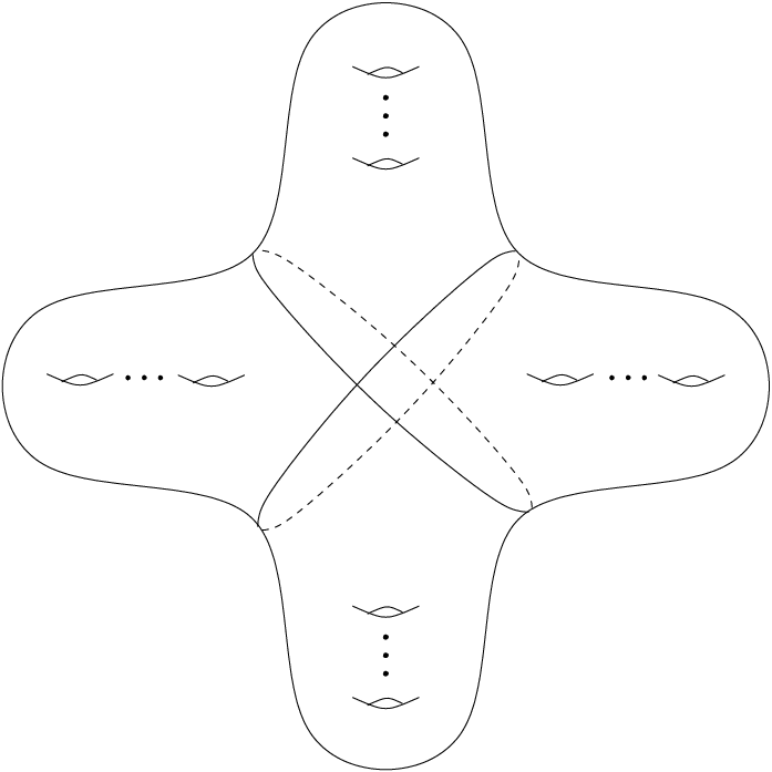
Lemma 2.3.

Suppose that $f\in\mathcal{I}(S)$ , that $c$ is a nonseparating curve, and that $f(c)\neq c$ . Then at least one of $i(f(c),c)$ and $i(f^{2}(c),c)$ is at least 2.

Note that this lemma is sharp for $g\geq 3$ in the sense that there exists an element $f\in\mathcal{I}(S)$ and a curve $c$ so that $i(c,f(c))=0$ and $i(c,f^{2}(c))=2$ . Consider, for instance, a bounding pair $\{d,e\}$ , i.e. a pair of disjoint, nonhomotopic, homologous, nonseparating simple closed curves, and a curve $c$ that intersects both $d$ and $e$ exactly once each; in this case, $i(c,T_{d}T_{e}^{-1}(c))=0$ and $i(c,(T_{d}T_{e}^{-1})^{2}(c))=2$ .

Proof.

Since $f\in\mathcal{I}(S)$ and $c\neq f(c)$ we know that $c\neq f^{2}(c)$ (combine Theorem 3 and Corollary 3.7 of [Iv2]). Now suppose $i(f(c),c)=0$ and $i(f^{2}(c),c)=0$ , so that $\{c,f(c),f^{2}(c)\}$ is a collection of 3 distinct, disjoint simple closed curves, each representing a fixed nonzero element of $H_{1}(S;\mathbb{Z})$ . We can choose curves $u_{2},v_{2},\dots,u_{g},v_{g}$ that are each disjoint from $c$ , $f(c)$ , and $f^{2}(c)$ , and whose corresponding homology classes span a codimension 2 subspace $V$ of $H_{1}(S;\mathbb{Z})$ . Now, $f$ takes the pair $\{c,f(c)\}$ to the pair $\{f(c),f^{2}(c)\}$ . However, it is clear that these two pairs induce different splittings of $V$ , and so we have a contradiction (see Figure 2). Since $f\in\mathcal{I}(S)$ , we cannot have $i(f(c),c)=1$ or $i(f^{2}(c),c)=1$ since these intersection numbers must be even, so we are done. ∎

Lemma 2.2 and Lemma 2.3 together prove Proposition 1.4, since a pseudo-Anosov mapping class does not fix any curve in the surface.

We require one final fact regarding geometric intersection numbers. Suppose $c$ and $c^{\prime}$ are homologous curves with $i(c,c^{\prime})=2$ . It follows that the two points of intersection must have opposite signs, and a regular neighborhood of $c\cup c^{\prime}$ is a 4 holed sphere. We orient $c$ and $c^{\prime}$ so that $[c]=[c^{\prime}]$ in $H_{1}(S;\mathbb{Z})$ . Label and orient the four boundary components of the 4 holed sphere $d$ , $d^{\prime}$ , $e$ and $e^{\prime}$ as in Figure 3.

Lemma 2.4.

Suppose $c$ and $c^{\prime}$ are homologous nonseparating curves with $i(c,c^{\prime})=2$ . Suppose that $d,d^{\prime}e$ and $e^{\prime}$ are the boundary components of a $4$ -holed sphere as shown in Figure 3. Then $d$ and $d^{\prime}$ are separating in $S$ , and $[e]=-[e^{\prime}]=[c]=[c^{\prime}]$ in $H_{1}(S;\mathbb{Z})$ .

Proof.

There are two pairs of pants in the 4 holed sphere which determine relations $[c]+[e^{\prime}]+[d^{\prime}]=0$ and $[c^{\prime}]+[e^{\prime}]+[d]=0$ . It follows that $[d]=[d^{\prime}]$ . Therefore $d\cup d^{\prime}$ is the boundary of two subsurfaces. The subsurface containing the 4 holed sphere is to the left of both $d$ and $d^{\prime}$ , so $[d]+[d^{\prime}]=0$ , and hence $[d]=[d^{\prime}]=0$ . A third pair of pants defines the relation $[c^{\prime}]-[e]-[d^{\prime}]=0$ , and so $[e]-[e^{\prime}]=[c]+[c^{\prime}]=2[c]\neq 0$ . Since the 4 holed sphere defines the relation $0=[e]+[e^{\prime}]+[d]+[d^{\prime}]$ and $[d]=[d^{\prime}]=0$ , we see that $[e]=-[e^{\prime}]=[c]=[c^{\prime}]$ . ∎

2.2 Proof of the lower bound

We begin by recalling a few definitions and facts; see [Ab] for a more detailed discussion. If $f$ is pseudo-Anosov, we let $q=q_{f}$ denote a holomorphic quadratic differential for which the vertical and horizontal foliations are precisely the stable and unstable foliations for $f$ , respectively. The differential $q$ determines a euclidean cone metric, which we also denote $q$ , and $f$ acts as an affine diffeomorphism (off the singularities) whose derivative has eigenvalues $\lambda(f)$ and $\lambda(f)^{-1}$ .

For any curve $c$ in $S$ , we let $\ell_{q}(c)$ denote the infimum of $q$ -lengths of representatives of $c$ , which is equivalently the length of a $q$ -geodesic representative for $c$ . We note that, in general, the $q$ -geodesic representative of a simple closed curve need not be embedded.

Lemma 2.5.

Let $f\in\Mod(S)$ be pseudo-Anosov and let $q=q_{f}$ . Then for any closed curve $c$ in $S$ , we have

\frac{\ell_{q}(f(c))}{\ell_{q}(c)}<\lambda(f).

Proof.

Note that because $f$ is affine with respect to $q$ , the image of a geodesic representative for $c$ is a geodesic representative for $f(c)$ . Furthermore, since the leading eigenvalue of the derivative of $f$ is $\lambda=\lambda(f)$ , the length of the curve $f(c)$ differs from that of $c$ by at most a factor of $\lambda$ . Moreover, only geodesics which are everywhere tangent to the eigenspace for $\lambda$ can be maximally stretched. However any such geodesic is a leaf of the stable or unstable foliation, and hence cannot be part of a closed geodesic, so the inequality is strict. ∎

We are now ready to give the proof of the lower bound on $L(\mathcal{I}(S))$ given in Theorem 1.1.

Proposition 2.6.

If $g\geq 2$ , then $L(\mathcal{I}(S_{g}))>.197$ .

Proof.

Let $f$ be an arbitrary pseudo-Anosov element of $\mathcal{I}(S)$ . Let $q=q_{f}$ , and let $c$ be a shortest curve in $S$ with respect to $q$ . We will assume in what follows that all closed $q$ -geodesics under consideration are embedded and that all pairs of $q$ -geodesics are in minimal position. This is not true in general, but so as not to disrupt the flow of ideas we make this assumption. We will discuss the minor modifications needed for the general case at the end of the proof.

Case 1. $i(c,f(c))\geq 4$ or $i(c,f^{2}(c))\geq 4$ .

Let $h$ be either $f$ or $f^{2}$ , where $i(c,h(c))\geq 4$ . The intersection points $c\cap h(c)$ cut each of $c$ and $h(c)$ into arcs. Since there are at least 4 intersection points, there is an arc $a$ of $h(c)$ which satisfies

\ell_{q}(a)\leq\frac{\ell_{q}(h(c))}{4}<\frac{\lambda(h)\ell_{q}(c)}{4}

where the second inequality comes from an application of Lemma 2.5. Here we have written $\ell_{q}(a)$ to denote the $q$ -length of the segment $a$ . The endpoints of $a$ cut $c$ into two arcs. One of which, call it $b$ , has length at most $\ell_{q}(c)/2$ . The union $a\cup b$ is a simple closed curve in $S$ . It is nontrivial for otherwise it would bound a disk, which we could use as a homotopy to show $i(c,h(c))<|c\cap h(c)|$ . Since $c$ is a shortest curve with respect to $q$ , we have

\begin{array}[]{rcl}\ell_{q}(c)\leq\ell_{q}(a\cup b)&\leq&\ell_{q}(a)+\ell_{q}(b)\\ &\\ &<&\displaystyle\frac{\lambda(h)\ell_{q}(c)}{4}+\frac{\ell_{q}(c)}{2}\\ &\\ &=&\ell_{q}(c)\left(\displaystyle\frac{\lambda(h)}{4}+\frac{1}{2}\right).\end{array}

It follows that

\frac{\lambda(h)}{4}+\frac{1}{2}>1

and so $\lambda(h)>2$ . Since $h$ is $f$ or $f^{2}$ and since $\lambda(f^{2})=\lambda(f)^{2}$ , we have $\lambda(f)>\sqrt{2}$ .

Case 2. $c$ is nonseparating and $i(c,f(c))$ and $i(c,f^{2}(c))$ are both less than 4.

By Lemma 2.3, either $i(c,f(c))=2$ or $i(c,f^{2}(c))=2$ . Let $h$ be either $f$ or $f^{2}$ , where $i(c,h(c))=2$ .

Let $d$ and $d^{\prime}$ be the separating curves from Lemma 2.4 with $c^{\prime}=h(c)$ . Alternatively, the intersection points $c\cap h(c)$ define 2 arcs of $c$ , say $a$ and $a^{\prime}$ , and two arcs of $h(c)$ , say $b$ and $b^{\prime}$ as in Figure 3. The curves $d$ and $d^{\prime}$ are then $d=a\cup b$ and $d^{\prime}=a^{\prime}\cup b^{\prime}$ .

Since

\begin{array}[]{rcl}\ell_{q}(a)+\ell_{q}(b)+\ell_{q}(a^{\prime})+\ell_{q}(b^{\prime})&=&\ell_{q}(c)+\ell_{q}(h(c))\\ &<&\ell_{q}(c)+\lambda(h)\ell_{q}(c)\end{array}

it follows that at least one of $d$ and $d^{\prime}$ , say $d$ , has length bounded above by half of $\ell_{q}(c)+\ell_{q}(h(c))$ :

\ell_{q}(d)<\frac{\ell_{q}(c)+\lambda(h)\ell_{q}(c)}{2}\leq\frac{\ell_{q}(c)+\lambda(f)^{2}\ell_{q}(c)}{2}.

(1)

We now consider $d$ , which is a separating curve, and its image $f(d)$ , which intersect in at least four points by Lemma 2.2. As in Case 1, if $a$ is the shortest arc of $f(d)$ and $b$ is the shortest arc of $d$ cut off by $a$ , then

\ell_{q}(a\cup b)<\ell_{q}(d)\left(\frac{\lambda(f)}{4}+\frac{1}{2}\right).

(2)

Note that we can always use $f$ (as opposed to $f^{2}$ ) since $d$ is separating.

Also, since $c$ is shortest, we have

\ell_{q}(c)\leq\ell_{q}(a\cup b).

(3)

Combining (1), (2), and (3) we see that

\ell_{q}(c)<\frac{\ell_{q}(c)+\lambda(f)^{2}\ell_{q}(c)}{2}\left(\frac{\lambda(f)}{4}+\frac{1}{2}\right).

In other words,

\lambda(f)^{3}+2\lambda(f)^{2}+\lambda(f)-6>0.

The cubic polynomial in $\lambda(f)$ on the left has one real root, and so

\lambda(f)>-\frac{2}{3}+\frac{1}{3}\sqrt[3]{82-9\sqrt{83}}+\frac{1}{3}\sqrt[3]{82+9\sqrt{83}}\approx 1.218

approximated from below.

By Proposition 1.4, these are all cases and so, after taking the logarithms, we are done if all $q$ -geodesics are embedded and all pairs are in minimal position.

In the general case, we approximate the $q$ -metric on $S$ by a nonpositively curved Riemannian metric $q_{0}$ which agrees with the $q$ -metric in the complement of a small neighborhood of the singular points. This can be done by an explicit computation; compare, e.g., [BH] or [GT]. Given any positive number $R>0$ , which is not one of the $q$ -lengths of a curve, we can choose this approximation so that the set of curves with $q$ -length at most $R$ is precisely the same as the set of curves with $q_{0}$ -length at most $R$ . Moreover, given $\epsilon>1$ , we may assume that the ratio of $q$ -length and $q_{0}$ -length of any curve is between $\epsilon$ and $1/\epsilon$ . In particular, since we can assume that $\lambda(f)\leq 2$ , say, then we may choose $q_{0}$ so that for the finite set of curves with $q_{0}$ -length at most $R$ , we have

\frac{\ell_{q_{0}}(f(c))}{\ell_{q_{0}}(c)}<\lambda(f).

Since a geodesic representative of any simple closed curve in a nonpositively curved Riemannian metric on a surface is embedded, and since any two representatives of distinct closed curves are in minimal position, choosing $R$ sufficiently large, the above proof can be carried out verbatim. ∎

For convenience, we isolate the key idea involved here as it will be used again.

Proposition 2.7.

If $f$ is a pseudo-Anosov element of $\Mod(S_{g})$ with the property that $i(c,f(c))\geq n\geq 3$ for every simple closed curve $c$ , then

\log(\lambda(f))>\log\left(\frac{n}{2}\right).

Proof.

As in the proof above, fix the metric $q=q_{f}$ on $S$ , and let $c$ be a shortest curve in $S$ with respect to $q$ . We again assume geodesics are embedded and pairs are in minimal position, with the general case handled as above. Take the shortest segment $a$ of $f(c)$ cut by $c$ (which is one of $i(c,f(c))$ segments of $f(c)$ ), and the shortest segment $b$ of $c$ cut by $a$ , and we obtain

\ell_{q}(c)\leq\ell_{q}(a\cup b)\leq\frac{\ell_{q}(f(c))}{i(c,f(c))}+\frac{\ell_{q}(c)}{2}<\frac{\lambda(f)\ell_{q}(c)}{i(c,f(c))}+\frac{\ell_{q}(c)}{2}.

Dividing the left and right by $\ell_{q}(c)$ , and simplifying and taking logarithms, we obtain

\log(\lambda(f))>\log\left(\frac{i(c,f(c))}{2}\right)\geq\log\left(\frac{n}{2}\right).

∎

Remark. Wolpert [Wo] has shown that a $K$ -quasiconformal map $f$ of $S$ with respect to a hyperbolic metric $X$ distorts lengths in $X$ by a factor of at most $K$ . That is, $\ell_{X}(f(c))/\ell_{X}(c)<K$ , where $\ell_{X}(c)$ is the length of $c$ with respect to $X$ . In a previous version we used this result and the same argument above (with no need for the final comment on minimal position and approximating Riemannian metrics) to produce a lower bound of $.197$ for $\log(\lambda^{2})$ . J. Franks suggested using the quadratic differential metric, thus improving the lower bound by a factor of $2$ .

2.3 Examples with small dilatation

In this section we give an upper bound for $L(\mathcal{I}(S))$ by constructing, for every $S=S_{g}$ ( $g\geq 2$ ), an element $f\in\mathcal{I}(S)$ with $\log(\lambda(f))<4.127$ . We do this by appealing to a general construction for pseudo-Anosov mapping classes given by Thurston [Th, §6]; we refer the reader to that paper for the notation and details of the construction.

A multicurve is the isotopy class of a collection of pairwise disjoint simple closed curves, and a multitwist is the product of Dehn twists about the curves in a multicurve.

We begin by fixing a pair of multicurves $A=a_{1}\cup\cdots\cup a_{\lceil g/2\rceil}$ and $B=b_{1}\cup\cdots\cup b_{\lceil g/2\rceil}$ in $S$ with the following three properties:

1.

$A\cup B$ fills $S$ .
2.

$i(a_{i},b_{i})=i(a_{i},b_{i-1})=4$ and $i(a_{i},b_{j})=0$ if $|i-j|>2$ (indices taken modulo $\lceil g/2\rceil$ ).
3.

Each $a_{i}$ and $b_{j}$ is a separating curve.

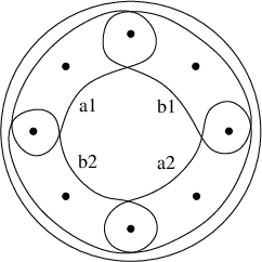
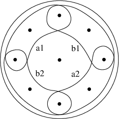
We can construct such an $A$ and $B$ explicitly as follows. Start with a sphere with $2g+2$ marked points arranged symmetrically as in Figure 4; the arrangement depends on whether $g$ is odd (on the left) or even (on the right—there is one more marked point “in back”). Let $\bar{A}=\cup\bar{a}_{i}$ and $\bar{B}=\cup\bar{b}_{i}$ be multicurves in the marked sphere as shown, and let $S$ be the two-fold cover, branched over the marked points, with $A$ and $B$ the preimages of $\bar{A}$ and $\bar{B}$ , respectively. Since each component of $\bar{A}$ and $\bar{B}$ surrounds exactly three marked points, each component of $A$ and $B$ is separating; in fact it bounds a genus $1$ subsurface.

Next, we consider the matrix $N_{ij}=i(a_{i},b_{j})$ , and compute the matrix $NN^{t}$ . This has entries given by

(NN^{t})_{ij}=\sum_{k=1}^{\lceil g/2\rceil}i(a_{i},b_{k})i(a_{j},b_{k})

and the above description of intersection numbers easily implies that for $i$ and $j$ modulo $\lceil g/2\rceil$ we have

(NN^{t})_{ij}=\left\{\begin{array}[]{rl}32&\quad\mbox{ for }\quad i=j\\ 16&\quad\mbox{ for }\quad|i-j|=1\\ 0&\quad\mbox{ for }\quad|i-j|\geq 2.\\ \end{array}\right.

In particular, note that the row sum of any row is $64$ . It follows that the Perron–Frobenius eigenvalue is $64$ : take as an eigenvector the vector with all entries equal to $1$ .

Now let $T_{A}$ denote the multitwist which is the composition of the Dehn twists about each of the $a_{i}$ and $T_{B}$ the composition of Dehn twists about each of the $b_{j}$ . In Thurston’s construction of pseudo-Anosov homeomorphisms mentioned above he begins by defining a homomorphism $\langle T_{A},T_{B}\rangle\to\PSL_{2}(\mathbb{R})$ which in this case is given by

T_{A}\mapsto\left(\begin{array}[]{rr}1&8\\ 0&1\\ \end{array}\right)\hskip 10.00002pt\mbox{ and }\hskip 10.00002ptT_{B}\mapsto\left(\begin{array}[]{rr}1&0\\ -8&1\\ \end{array}\right).

He then proves that any element of $\langle T_{A},T_{B}\rangle$ that maps to a hyperbolic element of $\PSL_{2}(\mathbb{R})$ is pseudo-Anosov. Moreover, the dilatation of such an element is given by the absolute value of the leading eigenvalue of its image.

Remark. Thurston’s construction of pseudo-Anosov homeomorphisms is much more general, merely requiring $A$ and $B$ to fill $S$ . In the general construction, the nonzero off-diagonal entries of the homomorphic images of $T_{A}$ and $T_{B}$ are given by the square root of the Perron–Frobenius eigenvalue of $NN^{t}$ . Again, $N$ is the matrix of intersection numbers of components of $A$ and $B$ .

In our case, a direct computation shows that the mapping class $f=T_{A}T_{B}$ maps to a matrix with trace $=-62$ . It follows that $f$ is pseudo-Anosov, and that $\lambda=\lambda(f)$ satisfies

\lambda^{2}-62\lambda+1=0.

Solving for the largest root, we find $\log(\lambda)<4.127$ . Since Dehn twists about separating curves are elements of $\mathcal{I}(S)$ , we have proven the upper bound of Theorem 1.1.

Proposition 2.8.

If $g\geq 2$ , then $L(\mathcal{I}(S_{g}))<4.127$ .

Remark. The map $T_{A}T_{B}$ has the smallest dilatation among all pseudo-Anosov elements of $\langle T_{A},T_{B}\rangle$ (see [Le]).

This construction also provides a universal upper bound for $L(PB_{n})$ for $n\geq 3$ .

Theorem 2.9.

For all $n\geq 3$ , we have

1.443<L(PB_{n})<2.634.

Proof.

As mentioned in the introduction, Song [So] proved the lower bound $1.443\approx\log(2+\sqrt{5})$ . For the upper bound, we start with the case where $n$ is odd, say $n=2g+1$ . To prove the upper bound, consider the sphere with marked points which we described above. We can puncture every marked point and turn one puncture into a boundary component, making the surface into a $(2g+1)$ -times punctured disk. Then $T_{\bar{A}}T_{\bar{B}}$ represents a pseudo-Anosov braid in $PB_{2g+1}$ . Indeed, we can use the same method of Thurston described above to find the homomorphism $\langle T_{\bar{A}},T_{\bar{B}}\rangle\to\PSL_{2}(\mathbb{R})$ . The eigenvalue for the analogous $NN^{t}$ matrix is 16, and so by a calculation, we obtain the upper bound

\log(\lambda(T_{\bar{A}}T_{\bar{B}}))<2.634.

We now do the case when $n$ is even. Whenever a marked point is not contained in a bigon, we can erase the marking, and $\bar{A}$ and $\bar{B}$ , as drawn, are still in minimal position. Puncturing the remaining marked points and turning one puncture into a boundary component, we can obtain examples proving the upper bound $L(PB_{n})<2.634$ for $n\geq 3$ . ∎

2.4 Principal congruence subgroups

We now give the proof of Theorem 1.7, which states that the bounds given in Propositions 2.6 and 2.8 for $L(\mathcal{I}(S))$ can be extended to $\Mod(S)[r]$ when $r\geq 3$ .

Question 2.10.

Is it true that $L(\Mod(S_{g})[2])\asymp 1$ ?

Proof of Theorem 1.7.

Since $\mathcal{I}(S)<\Mod(S)[r]$ , the upper bound is immediate. For $r\geq 4$ , the proof of the lower bound is essentially the same as that of Proposition 2.6; all that needs to be verified is that Lemmas 2.2 and 2.3 hold under the weaker hypothesis that $f\in\Mod(S)[r]$ , $r\geq 4$ . Indeed, the same arguments work, using splittings of $H_{1}(S;\mathbb{Z}/r\mathbb{Z})$ (and its quotients) in place of $H_{1}(S;\mathbb{Z})$ .

For the case $r=3$ , the proof is the same as in the $r\geq 4$ case, except we need to include the possibilities $i(c,f(c))=3$ and $i(c,f^{2}(c))=3$ in Case 1 of Proposition 2.6. By Proposition 2.7, the lower bound for this case becomes $.202>.197$ , and the argument for Case 2 still gives a lower bound of $.197$ , so we are done. ∎

It follows from the discreteness of $\spec(\Mod(S))$ , and the fact that $\mathcal{I}(S)<\Mod(S)[r]$ , that there is a (minimal) $r=r(g)$ such that $L(\Mod(S_{g})[n])=L(\mathcal{I}(S_{g}))$ whenever $n\geq r$ (see the proof of Proposition 4.1).

Question 2.11.

What are the values of $r(g)$ ? What are the asymptotics of $r(g)$ ?

3 The Johnson kernel

Johnson [Jo1] proved that $\mathcal{K}(S_{g})$ is an infinite index subgroup of $\mathcal{I}(S_{g})$ for $g\geq 3$ (when $g=2$ , the two groups agree). We have $L(\mathcal{K}(S))\geq L(\mathcal{I}(S))$ since $\mathcal{K}(S)<\mathcal{I}(S)$ , and it is natural to ask the following.

Question 3.1.

Is $L(\mathcal{K}(S_{g}))>L(\mathcal{I}(S_{g}))$ for $g\geq 3$ ?

While we do not know the answer to this question, we are able to give a better lower bound for $L(\mathcal{K}(S))$ than we did for $L(\mathcal{I}(S))$ in Theorem 1.1. As with $\mathcal{I}(S)$ , the key is to understand how elements of $\mathcal{K}(S)$ act on curves.

3.1 $\mathcal{K}(S)$ and geometric intersection numbers

The conclusions of Lemmas 2.2 and 2.3 can be improved by assuming $f\in\mathcal{K}(S)$ .

Proposition 3.2.

For $f\in\mathcal{K}(S)$ , and any curve $c$ , if $c\neq f(c)$ , then $i(c,f(c))\geq 4$ .

The proposition is sharp, since for $g\geq 2$ one can find a curve $c$ and a separating curve $d$ with $i(c,d)=2$ , and in this case $i(T_{d}(c),c)=4$ .

Proof.

When $c$ is separating the proposition was already proven in Lemma 2.2 for any $f\in\mathcal{I}(S)$ . So assume that $c$ is nonseparating. Since $f(c)$ is homologous to $c$ , it suffices to rule out $i(c,f(c))=0$ and $i(c,f(c))=2$ . As $\mathcal{K}(S)$ is normal in $\Mod(S)$ , the mapping class

[T_{c},f]=T_{c}fT_{c}^{-1}f^{-1}=T_{c}T_{f(c)}^{-1}

must lie in $\mathcal{K}(S)$ . The proposition now follows from Lemma 3.3 below. ∎

Lemma 3.3.

$\mathcal{K}(S)$ contains no elements of the form $T_{c}T_{d}^{-1}$ where $c$ and $d$ are distinct homologous curves with $i(c,d)$ either 0 or 2.

Proof.

Johnson [Jo1] constructed a homomorphism $\tau:\mathcal{I}(S)\to(\wedge^{3}H)/(\langle\omega\rangle\wedge H)$ , where $H=H_{1}(S;\mathbb{Z})$ and $\omega$ is the symplectic intersection pairing. He proved that the kernel is exactly $\mathcal{K}(S)$ . Moreover, Johnson [Jo1, Corollary to Lemma 4B] gave an explicit formula for the $\tau$ -image of a bounding pair map, i.e. a product of twists $T_{a}T_{b}^{-1}$ where $\{a,b\}$ is a bounding pair. For the formula, let $R$ be the component of $S-(a\cup b)$ not containing the base point for $\pi_{1}(S)$ , let $[a]$ denote the homology class of $a$ and $b$ (oriented so $R$ is to the left of $a$ ), and let $u_{1},v_{1}\dots,u_{k},v_{k}$ is any symplectic basis for $H_{1}(R;\mathbb{Z})/\langle[a]\rangle$ . The formula reads:

\tau(T_{a}T_{b}^{-1})=\left(\sum_{i=1}^{k}u_{i}\wedge v_{i}\right)\wedge[a].

(4)

It immediately follows that $\mathcal{K}(S)$ contains no bounding pair maps, and hence it remains to show that $\mathcal{K}(S)$ contains no elements of the form $T_{c}T_{d}^{-1}$ where $c$ and $d$ are homologous curves with $i(c,d)=2$ . By Lemma 2.4, $c$ and $d$ are necessarily configured as in Figure 5. Using the notation of the picture, the lantern relation (see [De, §7g]) gives

T_{e}T_{c}T_{d}=T_{x}T_{y}T_{z}T_{w}

which implies

T_{c}T_{d}^{-1}=T_{e}^{-1}T_{x}T_{y}T_{z}T_{w}T_{d}^{-2}.

As $T_{e}$ , $T_{x}$ , and $T_{y}$ are elements of $\mathcal{K}(S)$ , we see that $T_{c}T_{d}^{-1}$ is an element of $\mathcal{K}(S)$ if and only if $T_{z}T_{w}T_{d}^{-2}$ is an element of $\mathcal{K}(S)$ . The latter is a product of two bounding pair maps: $(T_{z}T_{d}^{-1})(T_{w}T_{d}^{-1})$ . To prove the lemma then, it suffices to check that $\tau(T_{z}T_{d}^{-1})\neq\tau(T_{d}T_{w}^{-1})$ . But this is apparent from equation (4) (consult Figure 5).

∎

3.2 Bounds for $L(\mathcal{K}(S))$

We are now ready to give the following improvement for the bounds on $L(\mathcal{K}(S))$ given by Theorem 1.1.

Proposition 3.4.

For $g\geq 2$ , we have

.693<L(\mathcal{K}(S_{g}))<4.127.

Proof.

The mapping class $T_{A}T_{B}$ constructed in §2.3 is a composition of Dehn twists about separating curves. Thus this mapping class already lies in $\mathcal{K}(S)$ , giving the upper bound. The lower bound follows immediately from Propositions 3.2 and 2.7, as $\log(2)\approx.693$ approximated from below. ∎

4 The Johnson filtration

We will now prove Theorem 1.2. Both the upper and lower bounds will follow from generalized versions of our arguments for $\mathcal{I}(S)$ and $\mathcal{K}(S)$ .

4.1 Asymptotic lower bounds

Before proving the lower bound in Theorem 1.2, we give the following weaker statement which holds for any normal filtration of $\Mod(S)$ , by which we mean a filtration of $\Mod(S)$ by normal subgroups.

Proposition 4.1.

For any normal filtration $N_{1}>N_{2}>\cdots$ of $\Mod(S)$ , we have $L(N_{k})\to\infty$ as $k\to\infty$ .

Proof.

Given $M>0$ , there are only finitely many conjugacy classes of pseudo-Anosov mapping classes $f$ with $\lambda(f)\leq M$ (see [Iv1]). The proposition then follows from the definition of a normal filtration. ∎

The first step towards the proof of Theorem 1.2 is to generalize Lemma 3.3. In the proof of this lemma, it was essential that there were unique pictures for homologous curves with geometric intersection number 0 or 2. We are forced to replace this precise description of how our two curves sit in $S$ with a rough finiteness statement.

A configuration is a triple $(S,c,d)$ , where $S$ is a closed surface, and $c$ and $d$ are distinct curves in $S$ which are in minimal position (i.e. their union does not bound any bigon). Let $N=N(c,d)$ denote a closed regular neighborhood of $c\cup d$ . There is a natural partial ordering on configurations where $(\hat{S},\hat{c},\hat{d})<(S,c,d)$ if $\hat{S}\not\cong S$ and there is a continuous map $\eta:(S,c,d)\to(\hat{S},\hat{c},\hat{d})$ which restricts to a homeomorphism of triples

\eta|_{N(c,d)}:(N(c,d),c,d)\to(N(\hat{c},\hat{d}),\hat{c},\hat{d}).

We call such a map $\eta$ a crushing map. Because the composition of crushing maps is a crushing map, $<$ is a partial order. Any minimal configuration with respect to this partial ordering is called a terminal configuration. We declare two configurations $(S,c,d)$ and $(\hat{S},\hat{c},\hat{d})$ to be equal provided they are homeomorphic as triples.

Lemma 4.2.

For every $n>0$ there are only finitely many terminal configurations $(S,c,d)$ with $i(c,d)\leq n$ .

Proof.

To begin, we show that the topology of the complement of $N(c,d)$ for any terminal configuration $(S,c,d)$ is limited.

Claim: If $(S,c,d)$ is terminal then every complementary component $U$ of $S-N(c,d)$ has genus at most one.

Proof of claim: Suppose $(S,c,d)$ is a configuration, and some component $U$ has genus at least two. We produce a crushing map $\eta:(S,c,d)\to(\hat{S},\hat{c},\hat{d})$ as follows. Let $\eta:S\to\hat{S}$ be the quotient of $S$ obtained by first fixing a compact genus 1 subsurface $R\subset U\subset S$ with exactly one boundary component and identifying (“crushing”) $R$ to a point. We let $\hat{c}=\eta(c)$ and $\hat{d}=\eta(d)$ and note that the restriction of $\eta$ to $N(c,d)$ is a homeomorphism onto $N(\hat{c},\hat{d})$ . To prove that $\eta$ is a crushing map, all that remains is to verify that $(\hat{S},\hat{c},\hat{d})$ is indeed a configuration. That is, we must check that $\hat{c}$ and $\hat{d}$ are essential, not homotopic to one another, and in minimal position. For this, it suffices to verify that no component of the complement of $N(\hat{c},\hat{d})$ is a disk or annulus if $\hat{c}\cap\hat{d}=\emptyset$ or a bigon if $\hat{c}\cap\hat{d}\neq\emptyset$ . However, the components of the complement of $N(\hat{c},\hat{d})$ are all homeomorphic to those of $N(c,d)$ with the exception of $\eta(U)$ , and since $c$ and $d$ are essential, homotopically distinct, and in minimal position, it suffices to verify this statement for the single component $\eta(U)$ . By construction, $\eta(U)$ has genus at least one, so it is not a disk, annulus, or bigon, and therefore $(\hat{S},\hat{c},\hat{d})$ is a configuration. It follows that $(\hat{S},\hat{c},\hat{d})<(S,c,d)$ , and $(S,c,d)$ is not terminal, proving the claim.

Now let $(S,c,d)$ be a terminal configuration with $N=N(c,d)$ . By Lemma 2.1, we have $\chi(N)=-i(c,d)\geq-n$ , and so there are finitely many possibilities for $N$ , up to homeomorphism. Since $c$ is a curve in $N$ , there are only finitely many possibilities for the homeomorphism type of $(N,c)$ . Further, since $c$ cuts $d$ into $i(c,d)\leq n$ arcs, it follows that there are only finitely many possibilities for the homeomorphism type of $(N,c,d)$ .

Now note that there are only finitely many possibilities for the number of boundary components of $N$ , and hence finitely many possibilities for the number of boundary components of $\overline{S-N}$ . Because each component of $\overline{S-N}$ has genus at most $1$ , there are only finitely many possibilities for the homeomorphism type of $\overline{S-N}$ . Finally, the homeomorphism type of $(S,c,d)$ can be specified by $\overline{S-N}$ and $(N,c,d)$ and the (finite) combinatorial gluing data matching boundary components of the former with those of the latter. ∎

The next lemma allows us to say that, given a particular terminal configuration $(S,c,d)$ with $T_{c}T_{d}^{-1}\in\mathcal{N}_{k}(S)$ , it is not possible to “push” $T_{c}T_{d}^{-1}$ further down the Johnson filtration by adding genus to $S$ outside $N(c,d)$ . The proof applies in a much more general context, so we state it in this generality.

Suppose we are given a map of pairs $\eta:(S,N)\to(\hat{S},\hat{N})$ where $N\subset S$ and $\hat{N}\subset\hat{S}$ are subsurfaces and the restriction $\eta|_{N}:N\to\hat{N}$ is a homeomorphism; for example $\eta$ might be a crushing map. Then any $f\in\Mod(S)$ which is supported in $N$ pushes forward via $\eta$ to an element $\hat{f}\in\Mod(\hat{S})$ supported in $\hat{N}$ given by $f|_{\hat{N}}=\eta|_{N}\circ f|_{N}\circ\eta|_{N}^{-1}$ .

Lemma 4.3.

Suppose $\eta:(S,N)\to(\hat{S},\hat{N})$ , $f\in\Mod(S)$ , and $\hat{f}\in\Mod(\hat{S})$ are as above. Then $\hat{f}\in\mathcal{N}_{k}(\hat{S})$ whenever $f\in\mathcal{N}_{k}(S)$ .

Proof.

Suppose that $f\in\mathcal{N}_{k}(S)$ , i.e. after picking a representative of $f$ and fixing a base point, the induced action $f_{\star}$ of $f$ on $\Gamma/\Gamma_{k}$ is inner (where $\Gamma=\pi_{1}(S)$ and $\Gamma_{k}$ is the $k^{\mbox{\tiny th}}$ term of its lower central series, as above).

Let $\hat{\Gamma}=\pi_{1}(\hat{S})$ , and denote by $\{\hat{\Gamma}_{i}\}$ its lower central series. The map $\eta$ induces a surjective homomorphism $\Gamma\to\hat{\Gamma}$ which restricts to a surjection $\Gamma_{k}\to\hat{\Gamma}_{k}$ , so we have an induced map $\eta_{\star}:\Gamma/\Gamma_{k}\to\hat{\Gamma}/\hat{\Gamma}_{k}$ . Finally, let $\hat{f}_{\star}$ be the induced action of $\hat{f}$ on $\hat{\Gamma}/\hat{\Gamma}_{k}$ . We encode this information in the following diagram.

The diagram is commutative by the definition of $\hat{f}_{\star}$ , which implies that $\hat{f}_{\star}$ is also inner; indeed, if $f_{\star}$ is conjugation by $\gamma$ , then $\hat{f}_{\star}$ is conjugation by $\eta_{\star}(\gamma)$ . Therefore, $\hat{f}\in\mathcal{N}_{k}(\hat{S})$ . ∎

We now arrive at the desired generalization of Lemma 3.3. Define

C(n)=1+\sup\{k\,|\,(S,c,d)\mbox{ is terminal, }i(c,d)\leq n\mbox{, and }T_{c}T_{d}^{-1}\in\mathcal{N}_{k}(S)\}

By Lemma 4.2 and the definition of a normal filtration, $C(n)$ is finite for each $n$ .

Lemma 4.4.

Let $n>0$ . If $c\neq d$ and $i(c,d)\leq n$ , then $T_{c}T_{d}^{-1}\notin\mathcal{N}_{C(n)}(S)$ . Furthermore, $\displaystyle\lim_{n\to\infty}C(n)=\infty$ .

Proof.

Suppose $c$ and $d$ are curves in $S$ with $i(c,d)\leq n$ and $T_{c}T_{d}^{-1}\in\mathcal{N}_{k}(S)$ . If $(S,c,d)$ is a terminal configuration, then by the definition of $C(n)$ , we see that $k<C(n)$ . If $(S,c,d)$ is not terminal, then there is a terminal configuration $(\hat{S},\hat{c},\hat{d})$ and crushing map $\eta:(S,c,d)\to(\hat{S},\hat{c},\hat{d})$ . The induced map of pairs $\eta:(S,N(c,d))\to(\hat{S},N(\hat{c},\hat{d}))$ and the map $T_{c}T_{d}^{-1}$ satisfy the hypothesis of Lemma 4.3 with

\widehat{T_{c}T_{d}^{-1}}=T_{\hat{c}}T_{\hat{d}}^{-1}

so $T_{\hat{c}}T_{\hat{d}}^{-1}\in\mathcal{N}_{k}(\hat{S})$ , which again implies $k<C(n)$ as required.

To complete the proof and show that $C(n)\to\infty$ , we first notice that $C(n)$ is nondecreasing, since the set of terminal configurations used to define $C(n)$ contains the set of configurations used to define $C(n-1)$ . Thus, it suffices to show that for any $k$ there exists a $c$ and $d$ such that $T_{c}T_{d}^{-1}\in\mathcal{N}_{k}(S)$ for some $S$ . Let $f\in\mathcal{N}_{k}(S)$ be any nontrivial element and $c$ any curve with $f(c)\neq c$ . Since $\mathcal{N}_{k}(S)\lhd\Mod(S)$ , it follows that $[T_{c},f]=T_{c}T_{f(c)}^{-1}$ is an element of $\mathcal{N}_{k}(S)$ . ∎

We are finally ready to give the “asymptotic version” of Proposition 3.2. For the statement, define

B(k)=\sup\{n:C(n)\leq k\}+1.

In the case where $B$ is not defined by this equation, we artificially set $B=0$ ( $B$ is not defined for any integer which is smaller than the smallest value of $C$ ). Note that $B(k)$ is well-defined and finite for each $k\geq 0$ since $C$ is unbounded and nondecreasing. Rephrasing, $B(k)$ is the minimum intersection number required for any pair of curves $c$ and $d$ in any surface $S$ to satisfy $T_{c}T_{d}^{-1}\in\mathcal{N}_{k}(S)$ .

We require the following alternate characterization of $B(k)$ , which follows immediately from the definition.

Lemma 4.5.

$B(k)$ is the smallest integer valued function for which $C(B(k))>k$ for all $k$ .

The next proposition gives the desired generalization of Proposition 3.2.

Proposition 4.6.

Let $k>0$ and let $S$ be any surface. If $f\in\mathcal{N}_{k}(S)$ , then $i(c,f(c))\geq B(k)$ for every simple closed curve $c$ in $S$ with $f(c)\neq c$ . Moreover, $\displaystyle\lim_{k\to\infty}B(k)=\infty$ .

Proof.

First, $B(k)\to\infty$ as $k\to\infty$ since $C$ is unbounded and nondecreasing. Now, given $k$ , choose any $S$ , any $f\in\mathcal{N}_{k}(S)$ , and any simple closed curve $c$ in $S$ with $f(c)\neq c$ . Since $\mathcal{N}_{k}(S)$ is normal in $\Mod(S)$ , we have $[T_{c},f]=T_{c}T_{f(c)}^{-1}\in\mathcal{N}_{k}(S)$ . By Lemma 4.5, if $i(c,f(c))<B(k)$ , then $C(i(c,f(c)))\leq k$ . By Lemma 4.4, we have $T_{c}T_{f(c)}^{-1}\notin\mathcal{N}_{k}(S)$ , which is a contradiction. ∎

Using Propositions 4.6 and 2.7, it is now straightforward to prove the lower bound of Theorem 1.2.

Proof of Theorem 1.2.

If $f\in\mathcal{N}_{k}(S)$ is pseudo-Anosov, then $i(c,f(c))\geq B(k)$ for every curve $c$ , by Proposition 4.6 and the fact that a pseudo-Anosov mapping class does not fix any curve. We set

m(k)=\log\left(\frac{B(k)}{2}\right).

By Proposition 2.7, $\log(\lambda(f))>m(k)$ , and so this completes the proof. ∎

Among several questions which now arise, we pose the following.

Question 4.7.

What are the asymptotics of $B(k)$ ? What are the asymptotics of $L(\mathcal{N}_{k}(S))$ ?

4.2 Asymptotic upper bounds

We now prove the upper bound in Theorem 1.2.

Proposition 4.8.

For any $k\geq 1$ , there is an $M(k)$ so that $L(\mathcal{N}_{k}(S_{g}))<M(k)$ for all $g\geq 2$ .

Since $m(k)\to\infty$ , it follows that $M(k)\to\infty$ as $k\to\infty$ .

Proof.

Let $k\geq 1$ be fixed. To prove the proposition, we need to find a pseudo-Anosov mapping class $f\in\mathcal{N}_{k}(S)$ whose dilatation depends on $k$ , but not on $S$ . We begin by recalling that since $\{\mathcal{N}_{i}(S)\}_{i\geq 1}$ is a central series for $\mathcal{I}(S)$ , then the $(k-1)^{\mbox{\tiny st}}$ term of the lower central series of $\mathcal{I}(S)$ is contained in $\mathcal{N}_{k}(S)$ ; note that $\mathcal{N}_{1}(S)=\mathcal{I}(S)$ is the zero term of the lower central series.

Now, without specifying a particular surface $S$ , we consider the group $\langle T_{A},T_{B}\rangle$ generated by the multitwists $T_{A}$ and $T_{B}$ of Section 2.3. The group $\langle T_{A},T_{B}\rangle$ is a free group on the given generators (see [Le, §6.1] for a discussion). Therefore, there is a nontrivial element $f$ in the $(k-1)^{\mbox{\tiny st}}$ term of the lower central series of $\langle T_{A},T_{B}\rangle$ . Since $T_{A}$ and $T_{B}$ are both elements of $\mathcal{I}(S)$ , it follows that $f$ is an element of the $(k-1)^{\mbox{\tiny st}}$ term of the lower central series of $\mathcal{I}(S)$ , and hence $f\in\mathcal{N}_{k}(S)$ .

The key feature here is this: the image of $f$ in $\PSL_{2}(\mathbb{R})$ does not depend of the choice of $S$ . This is because $f$ was chosen independently of $S$ as a word in $T_{A}$ and $T_{B}$ , and the images of $T_{A}$ and $T_{B}$ in $\PSL_{2}(\mathbb{R})$ do not depend on the choice of $S$ (see Section 2.3).

Since $\langle T_{A},T_{B}\rangle$ is a free group and the only elements of this group which are not pseudo-Anosov are conjugates of $T_{A}$ and $T_{B}$ (see, e.g., [Le]), it follows that $f$ is pseudo-Anosov. Since its dilatation only depends on its image in $\PSL_{2}(\mathbb{R})$ , and the latter is independent of the choice of $S$ , we are done. ∎

Remark. Note that the word in $T_{A}$ and $T_{B}$ given as a simple nested commutator has word length on the order of $2^{k}$ , where $k$ is the number of nested commutators involved (i.e. the depth in the lower central series). Thus the order of logarithm of the dilatation is at most exponential in $k$ .

5 Translation lengths on the complex of curves

Our goal in this section is to prove Theorems 1.5 and 1.6. These will follow rather quickly from Theorem 5.2.

We first need the following technical fact.

Lemma 5.1.

If $m,n\in\mathbb{Z}$ and $f\in\Mod(S)$ satisfy $n\tau_{\mathcal{C}}(f)>m$ , then $d_{\mathcal{C}}(f^{n}(c))\geq m+1$ for any curve $c$ .

Proof.

If not, we have $d_{\mathcal{C}}(f^{n}(c),c)\leq m$ , so by the triangle inequality $d_{\mathcal{C}}(f^{nj}(c),c)\leq mj$ . Dividing both sides by $nj$ and taking the $\liminf$ , we get

\liminf_{j\to\infty}\frac{d_{\mathcal{C}}(f^{nj}(c),c)}{nj}\leq\frac{m}{n}.

The $\liminf$ used to define $\tau_{\mathcal{C}}(f)$ is no larger than the left hand side, and so we arrive at $n\tau_{\mathcal{C}}(f)\leq m$ , a contradiction. ∎

Theorem 5.2.

For any $g\geq 2$ and any pseudo-Anosov $f\in\Mod(S_{g})$ with $\lambda(f)\leq g-1/2$ , we have

\tau_{\mathcal{C}}(f)<\frac{4\log(\lambda(f))}{\log\left(g-\frac{1}{2}\right)}.

Remark. It seems likely that the hypothesis $\lambda(f)\leq g-1/2$ is not necessary, but it is required for our argument.

Proof.

Let $n$ be the smallest integer so that $2<n\tau_{\mathcal{C}}(f)$ . Note that $n\tau_{\mathcal{C}}(f)\leq 4$ whenever $n>1$ .

Now, let $c$ be any curve in $S$ . By Lemma 5.1, $d_{\mathcal{C}}(f^{n}(c),c)\geq 3$ , which (by the definition of $d_{\mathcal{C}}$ ) implies that $c$ and $f^{n}(c)$ fill $S$ . Lemma 2.1 implies $i(c,f^{n}(c))\geq 2g-1$ , and hence Proposition 2.7 applied to $f^{n}$ says

n\log(\lambda(f))=\log(\lambda(f^{n}))>\log\left(g-\frac{1}{2}\right)

which we write as

\frac{1}{n}<\frac{\log(\lambda(f))}{\log\left(g-\frac{1}{2}\right)}.

By hypothesis, the right hand side is at most 1, and so $n>1$ . As mentioned above, this means that $n\tau_{\mathcal{C}}(f)\leq 4$ . Thus, we have

\tau_{\mathcal{C}}(f)\leq\frac{4}{n}<\frac{4\log(\lambda(f))}{\log\left(g-\frac{1}{2}\right)}.

∎

We can now deduce Theorems 1.5 and 1.6 as corollaries of Theorem 5.2.

Proof of Theorem 1.5.

Let $f_{g}\in\Mod(S_{g})$ be a minimal dilatation pseudo-Anosov mapping class. Hironaka–Kin [HK] showed that $\log(\lambda(f_{g}))\leq\log(2+\sqrt{3})/g$ , and so if $g\geq 3$ , then $\lambda(f_{g})<g-1/2$ . The theorem thus follows for $g\geq 3$ from Theorem 5.2. The case of genus 2 can be handled by explicit examples. ∎

Proof of Theorem 1.6.

For any fixed $k$ , with $M(k)$ as in Theorem 1.2, we have $M(k)\leq\log(g-1/2)$ for $g$ sufficiently large. That is, for large enough $g$ , we have some $f_{g}\in\mathcal{N}_{k}(S_{g})$ with $\lambda(f_{g})\leq g-1/2$ . Letting $g$ tend to infinity, Theorem 5.2 implies

L_{\mathcal{C}}(\mathcal{N}_{k}(S_{g}))\leq\tau_{\mathcal{C}}(f_{g})<\frac{4\log(\lambda(f_{g}))}{\log\left(g-\frac{1}{2}\right)}\leq\frac{4M(k)}{\log\left(g-\frac{1}{2}\right)}\to 0.

∎

6 Brunnian subgroups

Let $S_{g,p}$ be the orientable surface of genus $g$ with $p>0$ punctures, and let $\PMod(S_{g,p})$ be the subgroup of $\Mod(S_{g,p})$ consisting of elements which fix each puncture. There are $p$ natural surjective homomorphisms

F_{i}:\PMod(S_{g,p})\to\PMod(S_{g,p-1})

obtained by filling in the $i^{\mbox{\tiny th}}$ puncture, for $1\leq i\leq p$ . The Brunnian subgroup of $\Mod(S_{g,p})$ is the (nonempty!) intersection of the kernels:

\brun(S_{g,p})=\displaystyle\bigcap_{i=1}^{p}\textrm{ker}(F_{i}).

A topological description of each $F_{i}$ is given by the Birman exact sequence [Bi, Theorem 1.4].

Proof of Theorem 1.8.

This is similar to the proof of the lower bound in Proposition 2.6 and comes in two parts. We begin by uniformly bounding $i(c,f(c))$ from below for any $f\in\brun(S_{g,p})$ and any curve $c$ with $f(c)\neq c$ . To do this, we first note that by definition $F_{i}(f)(c)=c$ for every curve $c$ and every $i=1,...,p$ (since $F_{i}(f)=1$ ). In other words, if we fill in any puncture, $f(c)$ becomes isotopic to $c$ . Therefore, the complement of $c\cup f(c)$ contains $p$ punctured bigons, one for each puncture of $S_{g,p}$ . In the present case, an endpoint of a punctured bigon can lie in at most two punctured bigons and so we have $i(c,f(c))\geq p$ .

For the second part of the proof we would like to apply Proposition 2.7. However, this is unavailable: the hypothesis of that proposition requires that the surface involved be closed. Indeed, that proof breaks down when the surface has punctures since the curve which is produced by the cut-and-paste may be peripheral (homotopic to a puncture), and hence has no geodesic representative.

Proposition 6.1 below is a version of Proposition 2.7 for punctured surfaces, and it completes the proof. ∎

Proposition 6.1.

If $f\in\Mod(S_{g,p})$ is pseudo-Anosov and has the property that $i(c,f(c))\geq n\geq 5$ for every simple closed curve $c$ , then

\log(\lambda(f))>\log\left(\frac{n}{4}\right).

Proof.

As in the proof of Proposition 2.7, we let $q=q_{f}$ . In addition to the fact that the metric is singular and so geodesic representatives may not be in minimal position, there is another difficulty which arises in this setting. Namely, the presence of punctures makes the metric incomplete and geodesic representatives may not exist at all. We modify the metric to be a complete Riemannian metric to alleviate both of these problems. As in the proof of Proposition 2.6, we can change the metric in small neighborhoods of the singularities to be smooth and have nonpositive curvature. We can also modify the metric in a small neighborhood of the punctures to be nonpositively curved and complete by inserting a hyperbolic cusp and interpolating between the hyperbolic metric and flat metric by nonpositively curved metrics (again, by explicit computation).

Let $q_{0}$ denote the modified Riemannian metric of nonpositive curvature. We may thus assume that all $q_{0}$ –geodesics are embedded and pairs are in minimal position. Moreover, by choosing $q_{0}$ to approximate $q$ sufficiently well on large compact subsets of $S$ , we may assume that for all sufficiently short nonperipheral curves (in particular, all those curves that we will encounter)

\frac{\ell_{q_{0}}(f(c))}{\ell_{q_{0}}(c)}<\lambda(f).

We let $c$ be a shortest (nonperipheral) curve in the $q_{0}$ -metric and consider two arcs $a_{1}$ and $a_{2}$ of $f(c)$ cut along $c$ which share an endpoint, and for which

\ell_{q_{0}}(a_{1})+\ell_{q_{0}}(a_{2})\leq 2~\frac{\ell_{q_{0}}(f(c))}{i(c,f(c))}.

Let $b_{1}$ and $b_{2}$ be the shortest arcs of $c$ cut by $a_{1}$ and $a_{2}$ , respectively. We also consider the concatenated arc $a=a_{1}\cup a_{2}$ , and let $b$ denote the shortest arc of $c$ cut by $a$ .

Suppose now that $a_{1}\cup b_{1}$ , say, is not peripheral. Then as in the proof of Proposition 2.7 we obtain

\ell_{q_{0}}(c)\leq\ell_{q_{0}}(a_{1}\cup b_{1})<\frac{2\lambda(f)\ell_{q_{0}}(c)}{n}+\frac{\ell_{q_{0}}(c)}{2}

and hence

\log(\lambda(f))>\log\left(\frac{n}{4}\right).

Since each of $a_{1}$ , $a_{2}$ , and $a$ has length at most $2\ell_{q_{0}}(f(c))/i(c,f(c))$ , and each of $b_{1}$ , $b_{2}$ , and $b$ has length at most $\ell_{q_{0}}(c)/2$ , we obtain the same bound if any of $a\cup b$ , $a_{1}\cup b_{1}$ , or $a_{2}\cup b_{2}$ is nonperipheral. Thus the proof will be complete if we can show that this is the case.

We label the endpoints of $a_{1}$ and $a_{2}$ as $x,y$ and $y,z$ , respectively (so the endpoints of $a$ are $x$ and $z$ ). We also orient $c$ and $f(c)$ , thus assigning signs to the intersection points of $c\cap f(c)$ , and so in particular, to the points $x$ , $y$ , and $z$ . Two of the signs on $x$ , $y$ , and $z$ must agree. If $x$ and $y$ , say, have the same sign, then the curve $a_{1}\cup b_{1}$ is nonseparating since it has geometric intersection number $1$ with the curve $a_{1}\cup(c-b_{1})$ . Therefore, $a_{1}\cup b_{1}$ would be nonperipheral, and we would be done. Similarly, if $y$ and $z$ have the same sign, then $a_{2}\cup b_{2}$ is nonseparating and hence nonperipheral. Therefore, we may assume that the signs of intersection alternate.

It follows that a regular neighborhood of $a_{1}\cup a_{2}\cup c=a\cup c$ is as shown in Figure 6, where we have decomposed $c$ into three arcs $c_{1}\cup c_{2}\cup c_{3}$ by the intersection points $x$ , $y$ , and $z$ .

Each of the arcs $b_{1}$ , $b_{2}$ , and $b$ is made from unions of the three arcs $c_{1}$ , $c_{2}$ , and $c_{3}$ , depending on the relative lengths of $c_{1}$ , $c_{2}$ , and $c_{3}$ . There are three cases to consider.

Case 1. $\ell_{q_{0}}(c_{i})\leq\ell_{q_{0}}(c)/2$ for all $i=1,2,3$ .

In this case, we have $b_{1}=c_{1}$ , $b_{2}=c_{2}$ , and $b=c_{3}$ . Consider the regular neighborhood $N$ of $a\cup c$ shown in Figure 6. We claim that the inclusion of $N$ into $S$ injects on the level of fundamental groups, i.e. $N$ is incompressible. Recall the elementary fact that a subsurface is incompressible if and only if each of the boundary curves is homotopically nontrivial (i.e. none of the boundary curves is homotopic to a point). It follows that $N$ is incompressible since each of the boundary components is (homotopic to) a union of two segments in $c$ and $f(c)$ (which were in minimal position), hence homotopically nontrivial. Note furthermore that $a\cup b$ is not peripheral in $N$ , hence cannot be peripheral in $S$ .

Case 2. $\ell_{q_{0}}(c_{i})>\ell_{q_{0}}(c)/2$ for $i=1$ or $i=2$ .

We consider only the situation $\ell_{q_{0}}(c_{1})>\ell_{q_{0}}(c)/2$ , with the proof for $\ell_{q_{0}}(c_{2})>\ell_{q_{0}}(c)/2$ obtained by simply changing the labels. In this case, we have $b_{1}=c_{2}\cup c_{3}$ , $b_{2}=c_{2}$ , and $b=c_{3}$ . We now consider the regular neighborhood $N$ of $a\cup b_{1}=a\cup c_{2}\cup c_{3}$ , which is a pair of pants. Note that $a_{1}\cup b_{1}$ , $a_{2}\cup b_{2}$ , and $a\cup b$ are all contained in $N$ . In fact, these curves are precisely the three boundary components. Since each of these curves is a union of two segments in $c$ and $f(c)$ , these are homotopically nontrivial, and so as in Case 1, $N$ is incompressible. Finally, if all three curves were peripheral, the complement of $N$ in $S$ would have to be three once-punctured disks, and hence $S$ would be a thrice-punctured sphere. This is a contradiction since there are no pseudo-Anosov homeomorphisms of a thrice-punctured sphere. Thus, one of the curves must be nonperipheral.

Case 3. $\ell_{q_{0}}(c_{3})>\ell_{q_{0}}(c)/2$ .

In this final case, we must have $b_{1}=c_{1}$ , $b_{2}=c_{2}$ , and $b=c_{1}\cup c_{2}$ . Here we let $N$ be the regular neighborhood of $a\cup b=a_{1}\cup a_{2}\cup c_{1}\cup c_{2}$ . Again $N$ is a pair of pants, and it contains our three curves $a_{1}\cup b_{1}$ , $a_{2}\cup b_{2}$ , and $a\cup b$ . As above $a_{1}\cup b_{1}$ and $a_{2}\cup b_{2}$ are homotopic to two of the three boundary components, and are both homotopically nontrivial. If we show that the third boundary component, $d$ (the dotted curve in Figure 6), is homotopically nontrivial, then $a\cup b$ , which is an immersed essential curve in $N$ , will be nonperipheral, and this will complete the proof.

If $d$ is homotopically trivial, then it bounds a disk $D$ in $S$ . Since $D$ cannot contain the other two boundary components of $N$ , as these are nontrivial, it follows that $D$ must be “outside” of $d$ in Figure 6. We orient $f(c)$ so that it passes through $x$ , $y$ , and $z$ in that order. After passing through $z$ , $f(c)$ enters $D$ . Since $f(c)$ has no further intersection with $a_{1}$ , $a_{2}$ , $c_{1}$ , and $c_{2}$ other than the ones shown, it must cross $c_{3}$ upon leaving $D$ . But this creates a bigon between $c$ and $f(c)$ , contradicting our standing assumption on minimal position. It follows that $d$ cannot be homotopically trivial, and hence $N$ is incompressible and $a\cup b$ is nonperipheral, as required. ∎

We believe that a much stronger result is true; namely, that dilatations increase exponentially in the number of punctures for Brunnian pseudo-Anosov mapping classes.

Conjecture 6.2.

There exist constants $A,B>0$ so that

L(\brun(S_{g,p}))\geq Ap+B

for all $p\geq 1$ and any $g$ .

References

[FLP] Travaux de Thurston sur les surfaces, volume 66 of Astérisque. Société Mathématique de France, Paris, 1979. Séminaire Orsay, With an English summary.
[Ab] William Abikoff. The real analytic theory of Teichmüller space, volume 820 of Lecture Notes in Mathematics. Springer, Berlin, 1980.
[AY] Pierre Arnoux and Jean-Christophe Yoccoz. Construction de difféomorphismes pseudo-Anosov. C. R. Acad. Sci. Paris Sér. I Math., 292(1):75–78, 1981.
[BL] Hyman Bass and Alexander Lubotzky. Linear-central filtrations on groups. In The mathematical legacy of Wilhelm Magnus: groups, geometry and special functions (Brooklyn, NY, 1992), volume 169 of Contemp. Math., pages 45–98. Amer. Math. Soc., Providence, RI, 1994.
[Ba1] Max Bauer. Examples of pseudo-Anosov homeomorphisms. Trans. Amer. Math. Soc., 330(1):333–359, 1992.
[Ba2] Max Bauer. An upper bound for the least dilatation. Trans. Amer. Math. Soc., 330(1):361–370, 1992.
[Be] Lipman Bers. An extremal problem for quasiconformal mappings and a theorem by Thurston. Acta Math., 141(1-2):73–98, 1978.
[Bi] Joan S. Birman. Braids, links, and mapping class groups. Princeton University Press, Princeton, N.J., 1974. Annals of Mathematics Studies, No. 82.
[BH] Steven A. Bleiler and Craig D. Hodgson. Spherical space forms and Dehn filling. Topology, 35(3):809–833, 1996.
[Br] Peter Brinkmann. A note on pseudo-Anosov maps with small growth rate. Experiment. Math., 13(1):49–53, 2004.
[De] Max Dehn. Papers on group theory and topology. Springer-Verlag, New York, 1987. Translated from the German and with introductions and an appendix by John Stillwell, With an appendix by Otto Schreier.
[GT] M. Gromov and W. Thurston. Pinching constants for hyperbolic manifolds. Invent. Math., 89(1):1–12, 1987.
[HS] Ji-Young Ham and Won Taek Song. The minimum dilatation of pseudo-Anosov 5-braids. Preprint, arXiv:math.GT/0506295.
[H] W. J. Harvey. Boundary structure of the modular group. In Riemann surfaces and related topics: Proceedings of the 1978 Stony Brook Conference (State Univ. New York, Stony Brook, N.Y., 1978), volume 97 of Ann. of Math. Stud., pages 245–251, Princeton, N.J., 1981. Princeton Univ. Press.
[HK] Eriko Hironaka and Eiko Kin. A family of pseudo-Anosov braids with small dilatation. Algebr. Geom. Topol., 6:699–738 (electronic), 2006.
[Iv1] Nikolai V. Ivanov. Coefficients of expansion of pseudo-Anosov homeomorphisms. Zap. Nauchn. Sem. Leningrad. Otdel. Mat. Inst. Steklov. (LOMI), 167(Issled. Topol. 6):111–116, 191, 1988.
[Iv2] Nikolai V. Ivanov. Subgroups of Teichmüller modular groups, volume 115 of Translations of Mathematical Monographs. American Mathematical Society, Providence, RI, 1992. Translated from the Russian by E. J. F. Primrose and revised by the author.
[Jo1] Dennis Johnson. An abelian quotient of the mapping class group ${\cal I}_{g}$ . Math. Ann., 249(3):225–242, 1980.
[Jo2] Dennis Johnson. A survey of the Torelli group. In Low-dimensional topology (San Francisco, Calif., 1981), volume 20 of Contemp. Math., pages 165–179. Amer. Math. Soc., Providence, RI, 1983.
[Le] Christopher J. Leininger. On groups generated by two positive multi-twists: Teichmüller curves and Lehmer’s number. Geom. Topol., 8:1301–1359 (electronic), 2004.
[MM] Howard A. Masur and Yair N. Minsky. Geometry of the complex of curves. I. Hyperbolicity. Invent. Math., 138(1):103–149, 1999.
[Mc] Curtis T. McMullen. Polynomial invariants for fibered 3-manifolds and Teichmüller geodesics for foliations. Ann. Sci. École Norm. Sup. (4), 33(4):519–560, 2000.
[Mk] Hiroyuki Minakawa. Examples of pseudo-Anosov homeomorphisms with small dilatations. J. Math. Sci. Univ. Tokyo, 13(2):95–111, 2006.
[Pe] R. C. Penner. Bounds on least dilatations. Proc. Amer. Math. Soc., 113(2):443–450, 1991.
[So] Won Taek Song. Upper and lower bounds for the minimal positive entropy of pure braids. Bull. London Math. Soc., 37(2):224–229, 2005.
[SKL] Won Taek Song, Ki Hyoung Ko, and Jérôme E. Los. Entropies of braids. J. Knot Theory Ramifications, 11(4):647–666, 2002. Knots 2000 Korea, Vol. 2 (Yongpyong).
[Th] William P. Thurston. On the geometry and dynamics of diffeomorphisms of surfaces. Bull. Amer. Math. Soc. (N.S.), 19(2):417–431, 1988.
[Wo] Scott Wolpert. The length spectra as moduli for compact Riemann surfaces. Ann. of Math. (2), 109(2):323–351, 1979.
[Zh] A. Yu. Zhirov. On the minimum dilation of pseudo-Anosov diffeomorphisms of a double torus. Uspekhi Mat. Nauk, 50(1(301)):197–198, 1995.

Benson Farb:
Dept. of Mathematics, University of Chicago
5734 University Ave.
Chicago, IL 60637
E-mail: farb@math.uchicago.edu

Christopher J. Leininger:
Dept. of Mathematics, University of Illinois at Urbana-Champaign
273 Altgeld Hall, 1409 W. Green St.
Urbana, IL 61802
E-mail: clein@math.uiuc.edu

Dan Margalit:
Dept. of Mathematics, University of Utah
155 S 1440 East
Salt Lake City, UT 84112
E-mail: margalit@math.utah.edu

The lower central series and pseudo-Anosov dilatations

Abstract

1 Introduction

Torelli dilatations.

Theorem 1.1.

The Johnson filtration.

Theorem 1.2.

Question 1.3.

Proposition 1.4.

Translation lengths on the complex of curves.

Theorem 1.5.

Theorem 1.6.

Congruence subgroups.

Theorem 1.7.

Theorem 1.8.

Related results in the literature.

Acknowledgements.

2 Torelli groups

2.1 𝓘⁡(𝑺)\mathcal{I}(S) and geometric intersection numbers

Lemma 2.1.

Proof.

Lemma 2.2.

Proof.

Lemma 2.3.

Proof.

Lemma 2.4.

Proof.

2.2 Proof of the lower bound

Lemma 2.5.

Proof.

Proposition 2.6.

Proof.

Proposition 2.7.

Proof.

2.3 Examples with small dilatation

Proposition 2.8.

Theorem 2.9.

Proof.

2.4 Principal congruence subgroups

Question 2.10.

Proof of Theorem 1.7.

Question 2.11.

3 The Johnson kernel

Question 3.1.

3.1 𝓚⁡(𝑺)\mathcal{K}(S) and geometric intersection numbers

Proposition 3.2.

Proof.

Lemma 3.3.

Proof.

3.2 Bounds for L⁡(𝒦⁡(S))L(\mathcal{K}(S))

Proposition 3.4.

Proof.

4 The Johnson filtration

4.1 Asymptotic lower bounds

Proposition 4.1.

Proof.

Lemma 4.2.

Proof.

Lemma 4.3.

Proof.

Lemma 4.4.

Proof.

Lemma 4.5.

Proposition 4.6.

Proof.

Proof of Theorem 1.2.

Question 4.7.

4.2 Asymptotic upper bounds

Proposition 4.8.

Proof.

5 Translation lengths on the complex of curves

Lemma 5.1.

Proof.

Theorem 5.2.

Proof.

Proof of Theorem 1.5.

Proof of Theorem 1.6.

6 Brunnian subgroups

Proof of Theorem 1.8.

Proposition 6.1.

2.1 $\mathcal{I}(S)$ and geometric intersection numbers

3.1 $\mathcal{K}(S)$ and geometric intersection numbers

3.2 Bounds for $L(\mathcal{K}(S))$