Edgeworth Expansion of the Largest Eigenvalue Distribution Function of GUE and LUE

Leonard N. Choup Affiliation: Department of Mathematics Affiliation: University of California Affiliation: Davis, CA 95616, USA Affiliation: email: choup@math.ucdavis.edu

Abstract

We derive expansions of the Hermite and Laguerre kernels at the edge of the spectrum of the finite $n$ Gaussian Unitary Ensemble (GUE_n) and the finite $n$ Laguerre Unitary Ensemble (LUE_n), respectively. Using these large $n$ kernel expansions, we prove an Edgeworth type theorem for the largest eigenvalue distribution function of GUE_n and LUE_n. In our Edgeworth expansion, the correction terms are expressed in terms of the same Painlevé II function appearing in the leading term, i.e. in the Tracy-Widom distribution. We conclude with a brief discussion of the universality of these results.

1 Introduction

The limiting distribution function for the largest eigenvalues in orthogonal, unitary and symplectic random matrix ensembles have found many applications outside their initial discovery in random matrix theory, see, for example, [3, 4, 24] for recent reviews. In these applications it is important to have correction terms to the limiting distribution. For example, in statistics [12] the sample size is always finite; and to assess quantitatively the range of validity of limit laws, one needs finite $n$ correction terms. In classical probability, a similar issue arises in the application of the Central Limit Theorem (CLT) to finite $n$ problems. Here the two main results are the Berry-Esseen theorem and the Edgeworth expansion [6].

Recall if $S_{n}$ is a sum of i.i.d. random variables $X_{j}$ , each with mean $\mu$ and variance $\sigma^{2}$ , that the distribution $F_{n}$ of the normalized random variable $(S_{n}-n\mu)/(\sigma\sqrt{n})$ satisfies the Edgeworth expansion¹¹ 1 We assume, of course, the moments $\mathbb{E}(X_{j}^{k})$ , $k=3,\ldots,r$ , exist; and as well, the condition $\lim_{|\zeta|\rightarrow\infty}\sup|\varphi(\zeta)|<\infty$ where $\varphi$ is the characteristic function of $X_{j}$ , see [6].

F_{n}(x)-\Phi(x)=\phi(x)\sum_{j=3}^{r}n^{-\frac{1}{2}j+1}R_{j}(x)+o(n^{-\frac{1}{2}r+1})

(1.1)

uniformly in $x$ . Here $\Phi$ is the standard normal distribution with density $\phi$ , and $R_{j}$ are polynomials depending only on $\mathbb{E}(X_{j}^{k})$ but not on $n$ and $r$ (or the underlying distribution of the $X_{j}$ ).

Introduce

F^{G,L}_{n,2}(t)=\mathbb{P}_{G,L}(\lambda_{\textrm{max}}^{G,L}\leq t)

(1.2)

where $\lambda_{\textrm{max}}^{G,L}$ is the largest eigenvalue in GUE_n or LUE_n, respectively. (When the context is clear, we often drop the $G$ or $L$ .) To obtain a nontrivial limit theorem, we must, as is well known, define normalized random variables $\hat{\lambda}_{\textrm{max}}^{G,L}$ . We find it useful to “fine tune” our normalization (see also [12]),

	$\displaystyle\hat{\lambda}_{\textrm{max}}^{G}$	$\displaystyle:=$	$\displaystyle{\lambda_{\textrm{max}}^{G}-\left(2(n+c_{G})\right)^{1/2}\over 2^{-1/2}n^{-1/6}}\,,$		(1.3)
	$\displaystyle\hat{\lambda}_{\textrm{max}}^{L}$	$\displaystyle:=$	$\displaystyle{\lambda_{\textrm{max}}^{L}-4(n+c_{L})-2\alpha\over 2(2n)^{1/3}}$		(1.4)

where $c_{G,L}$ are constants (to be chosen later), and $\alpha$ is the parameter appearing in LUE_n. (That is, the parameter $\alpha$ appearing in the Laguerre polynomials $L_{n}^{\alpha}$ .) Then $\hat{\lambda}_{\textrm{max}}^{G,L}$ converge in distribution to GUE Tracy-Widom (commonly denoted $F_{2}$ ). In this paper we initiate the study of Edgeworth expansions for both GUE_n and LUE_n; that is, we find the analogue of (1.1) for $F_{n}^{G,L}-F_{2}$ . We now state our main results.

Our first result is an extension of the Plancherel-Rotach theorem for the Laguerre poynomials $L_{n}^{\alpha}$ . We set

\xi=(4n+2\alpha+2c)^{\frac{1}{2}}+\frac{X}{2^{\frac{2}{3}}n^{\frac{1}{6}}}\quad\textmd{where}\;X\;\textmd{and}\;c\;\textmd{are}\;\textmd{bounded},

(1.5)

and denote by $\airy$ the Airy function (see, e.g., [15]).

Theorem 1.1.

For $\alpha>-1$ we have as $n\rightarrow\infty$

e^{-\xi^{2}/2}L_{n}^{\alpha}(\xi^{2})=(-1)^{n}2^{-\alpha-\frac{1}{3}}n^{-\frac{1}{3}}\quad\left\{\airy(X)+\frac{(c-1)}{2^{\frac{1}{3}}}\airy^{\prime}(X)n^{-\frac{1}{3}}+\right.

\left[\frac{2-10c+5c^{2}-5\alpha}{10\cdot 2^{\frac{2}{3}}}\,X\airy(X)+\frac{X^{2}}{20\cdot 2^{\frac{2}{3}}}\airy^{\prime}(X)\right]n^{-\frac{2}{3}}+

\left[(\frac{5\alpha-15c\alpha+2c^{3}-15c^{2}-56c-6}{60}+\frac{c-1}{40}X^{3})\airy(X)+\right.

\left.\left.\frac{(c-1)(5(c-2)c-3(2+5\alpha))}{60}\,X\airy^{\prime}(X)\right]n^{-1}+O(n^{-\frac{4}{3}})\airy(X)\right\}

From Theorem 1.1 we derive expansions for both the Hermite and Laguerre kernels. Recall that if²² 2 Here $H_{n}(x)$ are the Hermite polynomials of degree $n$ .

\varphi_{n}(x)={1\over(2^{n}n!\sqrt{\pi})^{1/2}}\,H_{n}(x)\,e^{-x^{2}/2}\quad\textrm{and}\quad\phi_{n}^{\alpha}(x)=x^{\alpha/2}\,e^{-x/2}\,L_{n}^{\alpha}(x),

then the Hermite kernel is

K_{n}(x,y)=\sum_{k=0}^{n-1}\varphi_{k}(x)\varphi_{k}(y)

(1.6)

and the Laguerre kernel is

K_{n}^{\alpha}(x,y)=\sum_{k=0}^{n-1}\frac{\phi_{k}^{\alpha}(x)\phi_{k}^{\alpha}(y)}{\Gamma(k+1)\Gamma(\alpha+k+1)}\,.

(1.7)

Finally, the Airy kernel is

K_{\airy}(x,y)=\frac{\airy(x)\airy^{{}^{\prime}}(y)-\airy(y)\airy^{{}^{\prime}}(x)}{x-y}=\int_{0}^{\infty}\airy(x+z)\airy(y+z)\,dz.

(1.8)

Using Theorem 1.1 we prove

Theorem 1.2.

For $x=\left(2(n+c_{G})\right)^{\frac{1}{2}}+2^{-\frac{1}{2}}n^{-\frac{1}{6}}X$ and $y=\left(2(n+c_{G})\right)^{\frac{1}{2}}+2^{-\frac{1}{2}}n^{-\frac{1}{6}}Y$ with $X,\,Y$ and $c_{G}$ bounded,

\displaystyle K_{n}(x,y)\,dx=\left\{K_{\airy}(X,Y)-c_{G}\airy(X)\airy(Y)n^{-\frac{1}{3}}+\right.

\displaystyle\frac{1}{20}\left[(X+Y)\airy^{\prime}(X)\airy^{\prime}(Y)-(X^{2}+XY+Y^{2})\airy(X)\airy(Y)+\right.

\left.\left.\frac{-20c_{G}^{2}+3}{2}(\airy^{\prime}(X)\airy(Y)+\airy(X)\airy^{\prime}(Y))\right]n^{-\frac{2}{3}}+O(n^{-1})E(X,Y)\right\}\,dX.

(1.9)

The error term, $E(X,Y)$ , is the kernel of an integral operator on $L^{2}(J)$ which is trace class for any Borel subset $J$ of the reals that is bounded away from minus infinity.

For the Laguerre kernel we prove

Theorem 1.3.

For $x=4(n+c_{L})+2\alpha+2(2n)^{\frac{1}{3}}X$ and $y=4(n+c_{L})+2\alpha+2(2n)^{\frac{1}{3}}Y\;$ with $X$ , $Y$ and $c_{L}$ bounded,

\displaystyle K_{n}^{\alpha}(x,y)\,dx=\left\{K_{\airy}(X,Y)-2^{\frac{2}{3}}c_{L}\airy(X)\airy(Y)n^{-\frac{1}{3}}+\right.

\displaystyle\frac{2^{\frac{1}{3}}}{10}\left[\quad(X^{2}+X\,Y+Y^{2})\airy(X)\airy(Y)-(X+Y)\airy^{\prime}(X)\airy^{\prime}(Y)-\right.

\left.\left.(10c_{L}^{2}-1)(\airy(X)\airy^{\prime}(Y)+\airy^{\prime}(X)\airy(Y))\right]n^{-\frac{2}{3}}+O(n^{-1})F(X,Y)\right\}\,dX.

(1.10)

The error term $F(X,Y)$ is the kernel of an integral operator on $L^{2}(J)$ which is trace class for any Borel subset $J$ of the reals which is bounded away from minus infinity.

To state our main theorem, we need a number of definitions. First define the constants

a_{c_{G},2}^{G}=c_{G},\quad a_{c_{L},2}^{L}=2^{\frac{2}{3}}c_{L},\quad b_{2}^{G}=-\frac{1}{20},\quad b_{2}^{L}=\frac{2^{\frac{1}{3}}}{10}.

Following the notations of Tracy and Widom [20], we set

E_{c_{G},2}^{G}(s)=2w_{1}-3u_{2}+(-20c_{G}^{2}+3)v_{0}+u_{1}v_{0}-u_{0}v_{1}+u_{0}v_{0}^{2}-u_{0}^{2}w_{0},

\displaystyle E_{c_{L},2}^{L}(s)=2w_{1}-3u_{2}+(20c_{L}^{2}-2)v_{0}+u_{1}v_{0}-u_{0}v_{1}+u_{0}v_{0}^{2}-u_{0}^{2}w_{0},

where

u_{i}:=u_{i}(s)=\int_{s}^{\infty}q(x)x^{i}\airy(x)\,dx,\quad v_{i}:=v_{i}(s)=\int_{s}^{\infty}q(x)x^{i}\airy^{\prime}(x)\,dx\quad\textrm{and}

w_{i}:=w_{i}(s)=\int_{s}^{\infty}q^{\prime}(x)x^{i}\airy^{\prime}(x)\,dx\;+\;u_{0}(s)v_{i}(s)

with $q$ the solution of the Painlevé II equation, $q^{\prime\prime}=sq+2q^{3}$ , subject to the boundary condition $q(s)\sim\airy(s)$ as $s\rightarrow\infty$ . Finally, the GUE Tracy-Widom distribution is

F_{2}(s)=\det\left(I-K_{\airy}\raisebox{1.72218pt}{$\chi$}_{(s,\infty)}\right)=\exp\left(-\int_{s}^{\infty}(x-s)q(x)^{2}\,dx\right)

(1.11)

where $K_{\airy}$ is the operator with Airy kernel (1.8) and $\raisebox{1.72218pt}{$\chi$}_{(s,\infty)}$ is the indicator function of the interval $(s,\infty)$ . With now can state our main result.

Theorem 1.4.

We set

t=(2(n+c_{G}))^{\frac{1}{2}}+2^{-\frac{1}{2}}n^{-\frac{1}{6}}\,s\>\>\>\textrm{for GUE}_{n}

(1.12)

and

t=4(n+c_{L})+2\alpha+2(2n)^{\frac{1}{3}}\,s\>\>\>\textrm{for LUE}_{n}\,.

(1.13)

Then as $n\rightarrow\infty$

F_{n,2}^{G,L}(t)=F_{2}(s)\{1+a_{c_{G,L},2}^{G,L}\,u_{0}(s)\,n^{-\frac{1}{3}}+b_{2}^{G,L}E_{c_{G,L},2}^{G,L}(s)\,n^{-\frac{2}{3}}\}+O(n^{-1})

(1.14)

uniformly in $s$ . If in addition,

c_{G}^{2}+c_{L}^{2}=\frac{1}{4},\>\>\textrm{then}\>\>E_{{c_{G}},2}^{G}(s)=E_{{c_{L}},2}^{L}(s)=E_{c,2}(s),\>\>\textrm{and}

F_{n,2}^{G,L}(t)=F_{2}(s)\{1+a_{c_{G,L},2}^{G,L}\,u_{0}(s)\,n^{-\frac{1}{3}}+b_{2}^{G,L}E_{c,2}(s)\,n^{-\frac{2}{3}}\}+O(n^{-1}).

(1.15)

Note that the $n^{-\frac{1}{2}}$ correction term in the Edgeworth expansion for the CLT is universal in the sense that only the constant factor depends on the underlying distribution. We see in (1.15) a similar universality, and we conjecture that this universality extends to a wider class of unitary ensembles.

In §2 we derive Theorems 1.2 and 1.3 from Theorem 1.1. In §3 we follow [20] to prove Theorem 1.4. The proof of Theorem 1.1 will be given in the Appendices together with some facts needed to prove the last Theorem.

2 Correction terms for the Hermite and Laguerre kernel at the edge of the spectrum

To simplify notations we will use matrix ensembles of $(n+1)\times(n+1)$ matrices throughout this section and part of the next section. After the fine tuning of the variables in §3.3, we will use ensembles of $n\times n$ matrices.

2.1 Hermite case

We have the following representation of the Hermite kernel from the Christoffel-Darboux formula.

K_{n+1}(x,y)=\sqrt{\frac{n+1}{2}}\quad\frac{\varphi_{n+1}(x)\varphi_{n}(y)-\varphi_{n+1}(y)\varphi_{n}(x)}{x-y}

(2.1)

As mentioned in §1, Theorem 1.2 is a corollary of Theorem 1.1. We recall the relation between the Hermite and Laguerre polynomials

H_{2n}(x)=(-1)^{n}2^{2n}n!L_{n}^{-\frac{1}{2}}(x^{2}),\>\>H_{2n+1}(x)=(-1)^{n}2^{2n+1}n!xL_{n}^{\frac{1}{2}}(x^{2})

so as to estimate the right side of (2.1). We will also assume³³ 3 For $n$ odd the same analysis can be carried out to produce the same result. without lost of generalities that $n=2k$ is even. Using the symmetry of the Hermite kernel in (2.1) we only need to find an expansion of

\varphi_{n+1}(x)\varphi_{n}(y)=\frac{2^{4k+1}(k!)^{2}xe^{-\frac{x^{2}}{2}}L_{k}^{\frac{1}{2}}(x^{2})e^{-\frac{y^{2}}{2}}L_{k}^{-\frac{1}{2}}(y^{2})}{(2^{4k+1}(2k+1)!(2k)!\pi)^{\frac{1}{2}}}

(2.2)

since the other term follows by interchanging $x$ and $y$ . The Laguerre polynomial of argument $y$ in (2.2) has parameter $\alpha=-\frac{1}{2}$ ; thus, in order to apply Theorem 1.1, we write $y$ in the form $y=(4k-1+2c^{{}^{\prime}})^{\frac{1}{2}}+\frac{Y}{2^{\frac{2}{3}}k^{\frac{1}{6}}}$ which corresponds to $c^{{}^{\prime}}=c+1$ . Next we use Stirling’s formula to estimate

\quad\frac{2^{4k+1}(k!)^{2}x}{(2^{4k+1}(2k+1)!(2k)!\pi)^{\frac{1}{2}}}(-1)^{k}2^{-\frac{1}{2}-\frac{1}{3}}k^{-\frac{1}{3}}(-1)^{k}2^{\frac{1}{2}-\frac{1}{3}}k^{-\frac{1}{3}}\,.

The last factors in the left hand side are the constant factor in Theorem (1.1) for the Laguerre functions in $x$ and $y$ respectively. This expression is

\quad 2^{\frac{1}{3}}k^{-\frac{1}{6}}\left(1+\frac{X}{2^{\frac{5}{3}}k^{\frac{2}{3}}}+\frac{c}{4k}+O(k^{-\frac{5}{3}})\right).

This times, the constant⁴⁴ 4 Recall that in this section the notation $K_{n}$ stands for an ensemble of $(n+1)\times(n+1)$ matrices. $\sqrt{\frac{n+1}{2}}$ from (2.1), gives

2^{\frac{1}{3}}k^{\frac{1}{3}}(1+\frac{X}{2^{\frac{5}{3}}k^{\frac{2}{3}}}+\frac{c+1}{4k}+O(k^{-\frac{5}{3}})).

We substitute all these into (2.2), and then interchange $x$ and $y$ to have the second term $\varphi_{n+1}(y)\varphi_{n}(x)$ . Finally with the help of Mathematica we derive the following version of Theorem 1.2.

\textrm{For}\>\>x=(2n+1+2c)^{\frac{1}{2}}+\frac{X}{2^{\frac{1}{2}}n^{\frac{1}{6}}}\>\>\textrm{and}\>\>y=(2n+1+2c)^{\frac{1}{2}}+\frac{Y}{2^{\frac{1}{2}}n^{\frac{1}{6}}}\,,

(2.3)

\displaystyle K_{n+1}(x,y)dx=\left\{K_{\airy}(X,Y)+\frac{1-2c}{2}\airy(X)\airy(Y)n^{-\frac{1}{3}}+\left[\frac{X+Y}{20}\airy^{{}^{\prime}}(X)\airy^{{}^{\prime}}(Y)-\right.\right.

\displaystyle\left.\frac{X^{2}+XY+Y^{2}}{20}\airy(X)\airy(Y)+\frac{-10c^{2}+10c-1}{20}(\airy^{{}^{\prime}}(X)\airy(Y)+\airy(X)\airy^{{}^{\prime}}(Y))\right]n^{-\frac{2}{3}}

\left.+\,O(\,\frac{1}{n}\,)\;E(X,Y)\right\}dX

(2.4)

Using the symmetry between the $X$ and $Y$ terms from (2.1), this error term can be expressed as a finite sum

$\displaystyle E(X,Y)$	$\displaystyle=$	$\displaystyle\sum_{j}P_{j}(X,Y)\airy(X)\airy(Y)+\sum_{j_{1}}Q_{j_{1}}(X,Y)\airy^{{}^{\prime}}(X)\airy(Y)+$
		$\displaystyle\sum_{j_{2}}Q_{j_{2}}(X,Y)\airy(X)\airy^{{}^{\prime}}(Y)+\sum_{j}R_{j}(X,Y)\airy^{{}^{\prime}}(X)\airy^{{}^{\prime}}(Y)+$
		$\displaystyle\sum_{j,k}a_{j,k}\frac{X^{j}Y^{k}\airy(X)\airy^{{}^{\prime}}(Y)-X^{k}Y^{j}\airy^{{}^{\prime}}(X)\airy(Y)}{X-Y}$

where all coefficients of the polynomials $P$ , $Q$ and $R$ , and the $a_{j,k}$ have a factor of $n^{-\frac{1}{3}k}$ , $k\in\{0,1,2,3\}$ .

The first four terms are kernels of finite rank operators on any Borel subset $J$ of $\mathbb{R}$ not including minus infinity;⁵⁵ 5 This last restriction is due to the behavior of the Airy function near minus infinity. and thus, are trace class. The last term also defines a trace class operator. This is best seen from the following result. If we assumed without lost of generalities that $j\leq k$ , and set $k-j=s$ , then

			$\displaystyle\frac{X^{j}Y^{k}\airy(X)\airy^{{}^{\prime}}(Y)-X^{k}Y^{j}\airy^{{}^{\prime}}(X)\airy(Y)}{X-Y}$
		$\displaystyle=$	$\displaystyle(XY)^{j}\frac{(Y^{s}-X^{s}+X^{s})\airy(X)\airy^{{}^{\prime}}(Y)-X^{s}\airy^{{}^{\prime}}(X)\airy(Y)}{X-Y}$
		$\displaystyle=$	$\displaystyle(XY)^{j}\left(X^{s}K_{\airy}(X,Y)\;+\;\sum_{i=0}^{s-1}Y^{s-i}X^{i}\airy(X)\airy^{{}^{\prime}}(Y)\right).$

This shows that the error $E(X,Y)$ in (2.4) is the kernel of a trace class operator.

2.2 Laguerre case

Again by the Christoffel-Darboux formula,

K_{n+1}^{\alpha}(x,y)=\frac{(n+1)(xy)^{\frac{\alpha}{2}}}{\Gamma(\alpha+1)\left(\begin{array}[]{c}n+\alpha\\ n\\ \end{array}\right)}\frac{\phi_{n+1}^{\alpha}(x)\phi_{n}^{\alpha}(y)-\phi_{n+1}^{\alpha}(y)\phi_{n}^{\alpha}(x)}{x-y}\,.

(2.5)

2.2.1 Asymptotic of $e^{-\frac{x}{2}}L_{n}^{\alpha}(x)$ at $x=4n+2\alpha+2c+2(2n)^{\frac{1}{3}}X$

In order to apply Theorem 1.1 to the Laguerre kernel at the edge of the spectrum (corresponding to $x=4n+2\alpha+2c+2(2n)^{\frac{1}{3}}X$ for bounded $c$ and $X$ ), we need to make a variable change $x=\xi^{2}$ where $\xi=\sqrt{4n+2\alpha+2c}+\;2^{-\frac{2}{3}}n^{-\frac{1}{6}}\;t$ . We use these two expressions to solve for $t$ in terms of $X$ and then substitute this value for $t$ into Theorem 1.1 to obtain the desired asymptotics. But⁶⁶ 6 See the last footnote in the proof of Theorem 1.1 in the Appendix for this technical point. in order to have accurate asymptotics for the Laguerre functions at the edge of the spectrum, we will use the expression of $\xi$ involving $l_{n}=(4n+2\alpha+2c)^{1/2}$ . Thus

x=\xi^{2}\quad\textrm{is equivalent to }\quad l_{n}^{2}+2(2n)^{\frac{1}{3}}X=l_{n}^{2}+(2l_{n})^{\frac{2}{3}}t+(2l_{n})^{-\frac{2}{3}}t^{2}\;.

\displaystyle\textrm{This quadratic has solutions}\;t_{\pm}=\frac{1}{2}(-(2l_{n})^{\frac{4}{3}}\pm(2l_{n})^{\frac{4}{3}}\sqrt{1+4(2l_{n})^{-2}2(2n)^{\frac{1}{3}}X})\;.

Actually, only the solution with the plus sign is to be taken as it is the only one bounded when $n$ increases. An expansion of $t_{+}=t$ leads to:

\displaystyle t=X-\frac{(\alpha+c)}{6n}X-\frac{X^{2}}{2^{\frac{8}{3}}n^{\frac{2}{3}}}+O(n^{-\frac{4}{3}})\,.

Thus if in Theorem 1.1 we replace $X$ by this value of $t$ , we obtain, again with the help of Mathematica, the desired expansion.

Lemma 2.1.

For $\;x=4n+2\alpha+2c+2(2n)^{\frac{1}{3}}X$ and $X$ bounded,

e^{-\frac{x}{2}}L_{n}^{\alpha}(x)=(-1)^{n}2^{-\alpha-\frac{1}{3}}n^{-\frac{1}{3}}\left\{\airy(X)+\frac{(c-1)}{2^{\frac{1}{3}}}\airy^{{}^{\prime}}(X)n^{-\frac{1}{3}}+\right.

\left[\frac{2-10c+5c^{2}-5\alpha}{10\cdot 2^{\frac{2}{3}}}X\airy(X)-\frac{2X^{2}}{10\cdot 2^{\frac{2}{3}}}\airy^{{}^{\prime}}(X)\right]n^{-\frac{2}{3}}+

\frac{1}{60}\left[-\left(6+56c+15c^{2}-2c^{3}+5\alpha(3c-1)-6X^{3}+6cX^{3}\right)\airy(X)\right.

\left.\left.+\left(6+\alpha(5-15c)-6c-15c^{2}+5c^{3}\right)X\airy^{{}^{\prime}}(X)\right]n^{-1}\;+\;O(n^{-4/3})\,\airy(X)\right\}

(2.6)

2.2.2 Asymptotic of $e^{-\frac{x}{2}}L_{n+1}^{\alpha}(x)$ at $x=4n+2\alpha+2c+2(2n)^{\frac{1}{3}}X$

Making use of this last formula, we can derive an asymptotic for
$e^{-\frac{x}{2}}L_{n+1}^{\alpha}(x)$ when $x=4n+2\alpha+2c+2(2n)^{\frac{1}{3}}X$ . Note that the degree of the Laguerre polynomial is no longer $n$ but $n+1$ , so in order to use Lemma2.1, we need to write $x$ in terms of $n+1$ or $x=4(n+1)+2\alpha+2(c-2)+2(2(n+1))^{\frac{1}{3}}[X-\frac{1}{3n}X+O(n^{-2})]$ .
The substitution needed here is $c\rightarrow c-2\,$ , and $X\rightarrow X-\frac{1}{3n}X$ . Mathematica again gives:

Lemma 2.2.

For $x=4n+2\alpha+2c+2(2n)^{\frac{1}{3}}X$ and $X$ bounded,

\displaystyle e^{-\frac{x}{2}}L_{n+1}^{\alpha}(x)=(-1)^{n+1}2^{-\alpha-\frac{1}{3}}(n+1)^{-\frac{1}{3}}\left\{\airy(X)+\frac{(c-3)}{2^{\frac{1}{3}}}\airy^{{}^{\prime}}(X)n^{-\frac{1}{3}}+\right.

\displaystyle\left[\frac{42-30c+5c^{2}-5\alpha}{10\cdot 2^{\frac{2}{3}}}X\airy(X)-\frac{2X^{2}}{10\cdot 2^{\frac{2}{3}}}\airy^{{}^{\prime}}(X)\right]n^{-\frac{2}{3}}+

\displaystyle\frac{1}{60}\left[\left(30+28c-27c^{2}+2c^{3}-5\alpha(3c-7)+18X^{3}-6cX^{3}\right)\airy(X)\right.

\left.\left.+(-102-5\alpha(3c-7)+114c-45c^{2}+5c^{3})X\airy^{{}^{\prime}}(X)\right]n^{-1}\;+\;O(n^{-4/3})\,\airy(X)\right\}

(2.7)

To complete this subsection we need to estimate

\frac{(n+1)(xy)^{\frac{\alpha}{2}}}{\Gamma(\alpha+1)\left(\begin{array}[]{c}n+\alpha\\ n\\ \end{array}\right)}.

We have

\displaystyle(xy)^{\frac{\alpha}{2}}=2^{2\alpha}n^{\alpha}[1+\frac{\alpha(X+Y)}{2^{\frac{5}{3}}n^{\frac{2}{3}}}+\frac{\alpha(\alpha+c)}{2n}+O(n^{-\frac{4}{3}})],

\displaystyle\Gamma(\alpha+1)\left(\begin{array}[]{c}n+\alpha\\ n\\ \end{array}\right)=n^{\alpha}[1+\frac{\alpha^{2}+\alpha}{2n}+O(n^{-2})]

and in addition, the product of the constant factor on the right of (2.6) and (2.7) is

\displaystyle(-1)^{n+1}2^{-\alpha-\frac{1}{3}}(n+1)^{-\frac{1}{3}}\cdot(-1)^{n}2^{-\alpha-\frac{1}{3}}n^{-\frac{1}{3}}=-2^{-2\alpha}n^{-\frac{2}{3}}[1-\frac{1}{3n}+O(n^{-2})]

thus

\displaystyle\frac{(n+1)(xy)^{\frac{\alpha}{2}}}{\Gamma(\alpha+1)\left(\begin{array}[]{c}n+\alpha\\ n\\ \end{array}\right)}\cdot(-1)^{n+1}2^{-\alpha-\frac{1}{3}}(n+1)^{-\frac{1}{3}}\cdot(-1)^{n}2^{-\alpha-\frac{1}{3}}n^{-\frac{1}{3}}=

\displaystyle-2^{-\frac{2}{3}}n^{\frac{1}{3}}[1+\frac{\alpha(X+Y)}{2^{\frac{5}{3}}n^{\frac{2}{3}}}+\frac{3\alpha(c-1)+4}{6n}+O(n^{-\frac{4}{3}})]

Substituting all these quantities in (2.5), give the following version of Theorem 1.3

\textrm{For}\>\>x=4n+2\alpha+2c+2(2n)^{\frac{1}{3}}X\>\>\textrm{and}\>\>y=\ 4n+2\alpha+2c+2(2n)^{\frac{1}{3}}Y

(2.10)

\displaystyle K_{n+1}^{\alpha}(x,y)dx=\left\{K_{\airy}(X,Y)+\frac{2-c}{2^{\frac{1}{3}}}\,\airy(X)\,\airy(Y)\,n^{-\frac{1}{3}}+\right.

\displaystyle\frac{1}{2^{\frac{2}{3}}\,10}\left[2(X^{2}+X\,Y+Y^{2})\,\airy(X)\,\airy(Y)-\;2(X+Y)\,\airy^{{}^{\prime}}(X)\,\airy^{{}^{\prime}}(Y)-\right.

\left.\left.(18-20c+5c^{2})(\airy(X)\,\airy^{{}^{\prime}}(Y)+\airy^{{}^{\prime}}(X)\,\airy(Y))\right]n^{-\frac{2}{3}}+\,O(\,\frac{1}{n}\,)\;F(X,Y)\right\}dX.

(2.11)

As in the Hermite case, the error term $F(X,Y)$ is a finite sum of kernels of trace class operators, therefore is a kernel of a trace class operator on $L^{2}(J)$ for any subset $J$ of the reals which is bounded away from minus infinity.

2.3 Conclusion

For our order of expansion, we see that both kernels are finite rank perturbation of the Airy kernel. In the Laguerre case, the final result does not involve an explicit presence of the order $\alpha$ .

3 Expansion of the Fredholm determinants at the edge of the spectrum

This part will only make use (2.3) and (2.4) to derive the desired result in the Hermite case and (2.10) and (2.11) in the Laguerre case. Most of the derivations will follow from the work of Tracy and Widom.

3.1 Edgeworth expansion of $F_{n,2}^{G}$

Recall that

F_{n+1,2}^{G}(t)=\textrm{det}(I-K_{n+1})

(3.1)

where this determinant is the Fredholm determinant of the integral operator with kernel $K_{n+1}(x,y)$ on $L^{2}(s,\infty)$ , $t$ and $s$ are related by

t=(2\,n+1+2\,c)^{\frac{1}{2}}+2^{-\frac{1}{2}}\,n^{-\frac{1}{6}}\,s\,.

(3.2)

In this section we will estimate this determinant. Most of our derivations involve trace class operators where the Fredholm determinant is analytic. If in (3.1) we use the expression of $\;K_{n+1}\;$ given by (2.4), the continuity of the determinant (in trace class norm) allows us to pull the error term involving the kernel $E(X,Y)$ out of the determinant as an $O(n^{-1})$ term. We therefore have

\displaystyle\textrm{det}(I-K_{n+1})=\textrm{det}\left(I-\left\{K_{\airy}(X,Y)+\frac{1-2c}{2}\airy(X)\airy(Y)n^{-\frac{1}{3}}+\right.\right.

\displaystyle\left[\frac{X+Y}{20}\airy^{{}^{\prime}}(X)\airy^{{}^{\prime}}(Y)-\frac{X^{2}+XY+Y^{2}}{20}\airy(X)\airy(Y)+\right.

\left.\left.\left.\frac{-10c^{2}+10c-1}{20}(\airy^{{}^{\prime}}(X)\airy(Y)+\airy(X)\airy^{{}^{\prime}}(Y))\right]n^{-\frac{2}{3}}\right\}\right)+O(n^{-1}).

(3.3)

Note we are using the obvious notation of writing the kernel for the operator appearing in the determinant. We continue to employ this notation below. If we factor out $\textrm{det}(I-K_{\airy}(X,Y))$ and set

K_{n+1}(x,y)\,dx-K_{\airy}(X,Y)\,dX:=L(X,Y)\,dX+O(n^{-1})E(X,Y)\,dX,

the multiplicative property of the determinant gives

\textrm{det}(I-K_{n+1}(x,y))=\textrm{det}(I-K_{\airy}(X,Y))\textrm{det}(I-(I-K_{\airy}(X,Y))^{-1}L(X,Y))+O(n^{-1}).

(3.4)

The first factor on the right is known, so we need to estimate the second factor. We will express this factor as a finite sum of rank one operators

(I-K_{\airy}(X,Y))^{-1}L(X,Y)=\sum_{i=1}^{k}\alpha_{i}(X)\beta_{i}(Y)

(3.5)

and use the well known formula

\det\left(I-\sum_{i=1}^{k}\alpha_{i}(X)\beta_{i}(Y)\right)=\det\left(\delta_{ij}-(\alpha_{i},\beta_{j})\right)_{1\leq i,j\leq k}

(3.6)

to transform the problem to one involving estimations of inner products. Let $(\cdot,\cdot)$ denote the inner product in $L^{2}(s,\infty)$ . A good reference for much of the results that follows is [20]. We have the following representation.

\displaystyle(I-K_{\airy}(X,Y))^{-1}L(X,Y)=\frac{1-2c}{2}(I-K_{\airy}(X,Y))^{-1}\airy(X)\airy(Y)n^{-\frac{1}{3}}+

\displaystyle\frac{1}{20}\left[(I-K_{\airy}(X,Y))^{-1}X\airy^{{}^{\prime}}(X)\airy^{{}^{\prime}}(Y)+(I-K_{\airy}(X,Y))^{-1}Y\airy^{{}^{\prime}}(X)\airy^{{}^{\prime}}(Y)-\right.

\displaystyle(I-K_{\airy}(X,Y))^{-1}X^{2}\airy(X)\airy(Y)-(I-K_{\airy}(X,Y))^{-1}XY\airy(X)\airy(Y)-

\displaystyle(I-K_{\airy}(X,Y))^{-1}Y^{2}\airy(X)\airy(Y)+(-10c^{2}+10c-1)(I-K_{\airy}(X,Y))^{-1}\airy^{{}^{\prime}}(X)\airy(Y)

\displaystyle\left.+(-10c^{2}+10c-1)(I-K_{\airy}(X,Y))^{-1}\airy(X)\airy^{{}^{\prime}}(Y)\right]n^{-\frac{2}{3}}\,+\,O(n^{-1})

In the notations above, we think of all the quantities involved as kernels of integral operators, the analogues of those in [20]. We therefore have:

\displaystyle\frac{1-2c}{2}(I-K_{\airy}(X,Y))^{-1}\airy(X)\airy(Y)n^{-\frac{1}{3}}=\frac{1-2c}{2}Q(X)\airy(Y)n^{-\frac{1}{3}}:=\alpha_{1}(X)\beta_{1}(Y)

where $Q(X)$ is the action of the integral operator with kernel $(I-K_{\airy})^{-1}$ on $\airy(X)$ . In the same way we have,

	$\displaystyle\frac{1}{20}(I-K_{\airy}(X,Y))^{-1}X\airy^{{}^{\prime}}(X)\airy^{{}^{\prime}}(Y)n^{-\frac{2}{3}}=\frac{1}{20}((I-K_{\airy})^{-1}f)(X)\airy^{{}^{\prime}}(Y)n^{-\frac{2}{3}}$
	$\displaystyle:=\alpha_{2}(X)\beta_{2}(Y)$

where $f(Z)=Z\airy^{\prime}(Z)$ and,

	$\displaystyle\frac{1}{20}(I-K_{\airy}(X,Y))^{-1}\airy^{{}^{\prime}}(X)Y\airy^{{}^{\prime}}(Y)n^{-\frac{2}{3}}=\frac{1}{20}P(X)f(Y)n^{-\frac{2}{3}}$
	$\displaystyle:=\alpha_{3}(X)\beta_{3}(Y)$

where $P(X)$ is the action of the integral operator with kernel $(I-K_{\airy})^{-1}$ acting on $\airy^{{}^{\prime}}(X)$ .

	$\displaystyle-\frac{1}{20}(I-K_{\airy}(X,Y))^{-1}X^{2}\airy(X)\airy(Y)n^{-\frac{2}{3}}=-\frac{1}{20}((I-K_{Airy})^{-1}g)(x)\airy(y)n^{-\frac{2}{3}}$
	$\displaystyle:=\alpha_{4}(X)\beta_{4}(Y)$

where $g(Z)=Z^{2}\airy(Z)$ ,

	$\displaystyle-\frac{1}{20}(I-K_{\airy}(X,Y))^{-1}XY\airy(X)\airy(Y)n^{-\frac{2}{3}}=-\frac{1}{20}((I-K_{\airy})^{-1}h)(X)h(Y)n^{-\frac{2}{3}}$
	$\displaystyle:=\alpha_{5}(X)\beta_{5}(Y)$

where $h(Z)=Z\airy(Z)$ ,

\displaystyle-\frac{1}{20}(I-K_{\airy}(X,Y))^{-1}\airy(X)Y^{2}\airy(Y)n^{-\frac{2}{3}}=-\frac{1}{20}Q(X)g(Y)n^{-\frac{2}{3}}:=\alpha_{6}(X)\beta_{6}(Y)

\displaystyle C\,(I-K_{\airy}(X,Y))^{-1}\airy^{{}^{\prime}}(X)\airy(Y)n^{-\frac{2}{3}}=CP(X)\airy(Y)n^{-\frac{2}{3}}:=\alpha_{7}(X)\beta_{7}(Y)\,,\quad\textrm{and}

\displaystyle C\,(I-K_{\airy}(X,Y))^{-1}\airy(X)\airy^{{}^{\prime}}(Y)n^{-\frac{2}{3}}=CQ(X)\airy^{{}^{\prime}}(Y)n^{-\frac{2}{3}}:=\alpha_{8}(X)\beta_{8}(Y)

where $C=(-10c^{2}+10c-1)/20$ .

If we set $(\alpha_{i},\beta_{j})=a_{ij}n^{-\frac{2}{3}}$ for $j\neq 1$ and $(\alpha_{i},\beta_{1})=a_{i1}n^{-\frac{1}{3}}$ , expanding (3.6) with respect to the first row leads to the following expression.

$\displaystyle\textrm{det}(\delta_{ij}-(\alpha_{i},\beta_{j}))_{i,j=1}^{8}$	$\displaystyle=$	$\displaystyle(1-a_{11}n^{-\frac{1}{3}})\left\|\begin{array}[]{cccc}1-a_{22}n^{-\frac{2}{3}}&-a_{23}n^{-\frac{2}{3}}&\cdots&-a_{28}n^{-\frac{2}{3}}\\ -a_{32}n^{-\frac{2}{3}}&1-a_{33}n^{-\frac{2}{3}}&\cdots&-a_{38}n^{-\frac{2}{3}}\\ \cdot&\cdot&\cdot&\cdot\\ -a_{82}n^{-\frac{2}{3}}&-a_{83}n^{-\frac{2}{3}}&\cdots&1-a_{88}n^{-\frac{2}{3}}\\ \end{array}\right\|$
	$\displaystyle+$	$\displaystyle\sum_{k=2}^{8}(-1)^{k}a_{1k}n^{-\frac{2}{3}}\textrm{det}(C_{1},\cdots,\hat{C_{k}},\cdots,C_{8})$
	$\displaystyle=$	$\displaystyle(1-a_{11}n^{-\frac{1}{3}})\left\|\begin{array}[]{cccc}1-a_{22}n^{-\frac{2}{3}}&-a_{23}n^{-\frac{2}{3}}&\cdots&-a_{28}n^{-\frac{2}{3}}\\ -a_{32}n^{-\frac{2}{3}}&1-a_{33}n^{-\frac{2}{3}}&\cdots&-a_{38}n^{-\frac{2}{3}}\\ \cdot&\cdot&\cdot&\cdot\\ -a_{82}n^{-\frac{2}{3}}&-a_{83}n^{-\frac{2}{3}}&\cdots&1-a_{88}n^{-\frac{2}{3}}\\ \end{array}\right\|$
	$\displaystyle+$	$\displaystyle O(n^{-1}).$

We factor out $n^{-\frac{1}{3}}$ from column $C_{1}$ in the last step. The determinant in the last line is of the same form as the the original determinant, therefore a similar transformation to this last determinant leads to the following result.

$\displaystyle\det\left(\delta_{ij}\right.$	$\displaystyle-$	$\displaystyle\left.(\alpha_{i},\beta_{j})\right)_{1\leq i,j\leq 8}=(1-a_{11}n^{-\frac{1}{3}})\prod_{k=2}^{8}(1-a_{kk}n^{-\frac{2}{3}})+O(n^{-1})$
	$\displaystyle=$	$\displaystyle(1-a_{11}n^{-\frac{1}{3}})\sum_{k=0}^{7}(-1)^{k}n^{-\frac{2k}{3}}\sum_{i_{1},\cdots,i_{k};i_{r}\neq i_{s}\in\{2,\dots,8\}}\quad\prod_{j=1}^{k}a_{i_{j}i_{j}}+O(n^{-1})$
	$\displaystyle=$	$\displaystyle 1-a_{11}n^{-\frac{1}{3}}-n^{-\frac{2}{3}}\sum_{k=2}^{8}a_{kk}+O(n^{-1})=1-\sum_{k=1}^{8}(\alpha_{k},\beta_{k})+O(n^{-1}).$

Thus we only need to compute the inner products $(\alpha_{k},\beta_{k})\;\textrm{for}\;k=1,\cdots,8$ .
To simplify notations we will write for example $u_{0}$ instead of $u_{0}(s)$ . We therefore have:

\displaystyle(\alpha_{1},\beta_{1})

\displaystyle=

\displaystyle\frac{1-2c}{2}(Q,\airy)n^{-\frac{1}{3}}=\frac{1-2c}{2}\,u_{0}\,n^{-\frac{1}{3}}

\displaystyle(\alpha_{2},\beta_{2})

\displaystyle=

\displaystyle\frac{n^{-\frac{2}{3}}}{20}((I-K_{\airy})^{-1}X\airy^{{}^{\prime}},\airy{{}^{\prime}})=\frac{n^{-\frac{2}{3}}}{20}(P,X\airy^{{}^{\prime}})=\frac{n^{-\frac{2}{3}}}{20}w_{1}

\displaystyle(\alpha_{3},\beta_{3})

\displaystyle=

\displaystyle\frac{n^{-\frac{2}{3}}}{20}(P,X\airy^{{}^{\prime}})=\frac{n^{-\frac{2}{3}}}{20}w_{1}

\displaystyle(\alpha_{4},\beta_{4})

\displaystyle=

\displaystyle-\frac{n^{-\frac{2}{3}}}{20}((I-K_{\airy})^{-1}g,\airy)=-\frac{n^{-\frac{2}{3}}}{20}(Q,X^{2}\airy)=-\frac{n^{-\frac{2}{3}}}{20}u_{2}

\displaystyle(\alpha_{5},\beta_{5})

\displaystyle=

\displaystyle-\frac{n^{-\frac{2}{3}}}{20}((I-K_{\airy})^{-1}h,h)=-\frac{n^{-\frac{2}{3}}}{20}(Q_{1},X\airy)

\displaystyle(\alpha_{6},\beta_{6})

\displaystyle=

\displaystyle-\frac{n^{-\frac{2}{3}}}{20}(Q,X^{2}\airy)=-\frac{n^{-\frac{2}{3}}}{20}u_{2}

\displaystyle(\alpha_{7},\beta_{7})

\displaystyle=

\displaystyle Cn^{-\frac{2}{3}}(P,\airy)=Cn^{-\frac{2}{3}}(Q,\airy^{{}^{\prime}})=Cn^{-\frac{2}{3}}v_{0}\quad=\quad(\alpha_{8},\beta_{8}).

To estimate $(\alpha_{5},\beta_{5})$ , we use equation 2.12 of [20] which says

Q_{1}(X)=XQ(X)+u_{0}P(X)-v_{0}Q(X),\quad\textrm{to have}

$\displaystyle(Q_{1}(X),X\airy(X))$	$\displaystyle=$	$\displaystyle(X\,Q(X)+u_{0}P(X)-v_{0}Q(X),X\airy(X))$
	$\displaystyle=$	$\displaystyle u_{2}-v_{0}u_{1}+u_{0}(P(X),X\airy(X))$
	$\displaystyle=$	$\displaystyle u_{2}-v_{0}u_{1}+u_{0}\widetilde{v}_{1}$
	$\displaystyle=$	$\displaystyle u_{2}-v_{0}u_{1}+u_{0}v_{1}-u_{0}v_{0}^{2}+u_{0}^{2}w_{0}.\quad(\textrm{ We used }\,(2.14)\,\textrm{ of }\cite[cite]{[\@@bibref{}{Trac7}{}{}]})$

And

(\alpha_{5},\beta_{5})=-\frac{n^{-\frac{2}{3}}}{20}(u_{2}-u_{1}v_{0}+u_{0}v_{1}-u_{0}v_{0}^{2}+u_{0}^{2}w_{0}).

Substituting this into the formula for the determinant gives

			$\displaystyle\textrm{det}(\delta_{ij}-(\alpha_{i},\beta_{j}))_{1\leq i,j\leq 8}=1-\sum_{k=1}^{8}(\alpha_{k},\beta_{k})+O(n^{-1})$
		$\displaystyle=$	$\displaystyle 1-\frac{1-2c}{2}u_{0}n^{-\frac{1}{3}}-\frac{n^{-\frac{2}{3}}}{20}\left\{2w_{1}-3u_{2}+(-20c^{2}+20c-2)v_{0}+u_{1}v_{0}\right.$
			$\displaystyle-\left.u_{0}v_{1}+u_{0}v_{0}^{2}-u_{0}^{2}w_{0}\right\}\quad+\quad O(n^{-1}).$

If we set

a_{c,2}^{G}(s)=\frac{2c-1}{2}\;,\quad b^{G}_{2}=-\frac{1}{20}\quad\textrm{and}

E_{c,2}^{G}(s)=2w_{1}-3u_{2}+(-20c^{2}+20c-2)v_{0}+u_{1}v_{0}-u_{0}v_{1}+u_{0}v_{0}^{2}-u_{0}^{2}w_{0},

(3.9)

equation (3.4) gives

Lemma 3.1.

For $t_{c}=(2n+1+2c)^{\frac{1}{2}}+2^{-\frac{1}{2}}\,n^{-\frac{1}{6}}\,s$ ,

F_{n+1,2}^{G}(t_{c})=F_{2}(s)\left\{1+a_{c,2}^{G}\,u_{0}(s)\,n^{-\frac{1}{3}}+b_{2}^{G}\,E_{c,2}^{G}(s)\,n^{-\frac{2}{3}}\right\}+O(n^{-1})

(3.10)

For $c=\frac{1}{2}$ we have faster convergence in Lemma 3.1 since $\;a_{\frac{1}{2},2}^{G}=0$ .

3.2 Edgeworth Expansion of $F_{n,2}^{L}$

From the similarities between the two expressions in (2.4) and (2.11), the derivation of $F_{n+1,2}^{L}$ follows exactly the same steps as the previous one, they would differ only by some constant terms.

We see that the corresponding inner products in terms of the $\alpha$ ’s are

	$\displaystyle(\alpha_{1},\beta_{1})=\frac{2-c}{2^{\frac{1}{3}}}u_{0}n^{-\frac{1}{3}}\quad,\quad(\alpha_{5},\beta_{5})=-\frac{n^{-\frac{2}{3}}}{2^{\frac{2}{3}}\cdot 10}2w_{1}\quad,\quad(\alpha_{6},\beta_{6})=-\frac{n^{-\frac{2}{3}}}{2^{\frac{2}{3}}\cdot 10}2w_{1},$
	$\displaystyle(\alpha_{2},\beta_{2})=\frac{n^{-\frac{2}{3}}}{2^{\frac{2}{3}}\cdot 10}2u_{2}\quad,\quad(\alpha_{3},\beta_{3})=\frac{n^{-\frac{2}{3}}}{2^{\frac{2}{3}}\cdot 10}2(u_{2}-u_{1}v_{0}+u_{0}v_{1}-u_{0}v_{0}^{2}+u_{0}^{2}w_{0}),$
	$\displaystyle(\alpha_{4},\beta_{4})=\frac{n^{-\frac{2}{3}}}{2^{\frac{2}{3}}\cdot 10}2u_{2}\quad,\quad(\alpha_{7},\beta_{7})=-\frac{n^{-\frac{2}{3}}}{2^{\frac{2}{3}}\cdot 10}(18-20c+5c^{2})v_{0}=(\alpha_{8},\beta_{8}).$

If we set

a_{c,2}^{L}(s)=\frac{c-2}{2^{\frac{1}{3}}}\;,\quad b^{L}_{2}=\frac{2^{\frac{1}{3}}}{10}\quad\textrm{and}

E_{c,2}^{L}(s)=2w_{1}-3u_{2}+(5c^{2}-20c+18)v_{0}+u_{1}v_{0}-u_{0}v_{1}+u_{0}v_{0}^{2}-u_{0}^{2}w_{0},

(3.11)

our formula reads

Lemma 3.2.

For $t_{c}=4n+2\alpha+2c+2(2n)^{\frac{1}{3}}s$ ,

F_{n+1,2}^{L}(t_{c})=F_{2}(s)\{1+a_{c,2}^{L}\,u_{0}(s)\,n^{-\frac{1}{3}}+b_{2}^{L}\,E_{c,2}^{L}(s)\,n^{-\frac{2}{3}}\}\quad+\quad O(n^{-1}).

(3.12)

For $c=2$ we obtain a faster convergence as $a_{2,2}^{L}=0$ .

3.3 Fine tuning

To complete this analysis, we need to find values for the constant $\;c=c_{1}\;$ in Lemma 3.1 and $\;c=c_{2}\;$ in Lemma 3.2 for which $\quad E_{c_{1},2}^{G}(s)=E_{c_{2},2}^{L}(s)$ . Which is equivalent to

-20c_{1}^{2}+20c_{1}-2=5c_{2}^{2}-20c_{2}+18\quad\Leftrightarrow\quad(c_{1}-\frac{1}{2})^{2}+\frac{1}{4}(c_{2}-2)^{2}=\frac{1}{4}

(3.13)

This suggest the following change of variables.

c_{G}=c_{1}-\frac{1}{2}\quad\textrm{and}\quad c_{L}=\frac{c_{2}-2}{2}.\quad\textrm{Therefore}

\eqref{ellipse}\quad\textrm{ changes to }\quad c_{G}^{2}+c_{L}^{2}=\frac{1}{4}\;,\quad a_{c_{G},2}^{G}=c_{G}\,,\quad a_{c_{L},2}^{L}=2^{\frac{2}{3}}c_{L}\;,

-20c_{1}^{2}+20c_{1}-2\;=\;-20c_{G}^{2}+3\;,\quad 5c_{2}^{2}-20c_{2}+18\;=\;20c_{L}^{2}-2\;,

t_{c_{G}}=(2(n+1)+2c_{G})^{\frac{1}{2}}+2^{-\frac{1}{2}}n^{-\frac{1}{6}}s\quad\textrm{and}\quad t_{c_{L}}=4(n+1)+2\alpha+4c_{L}+2(2n)^{\frac{1}{3}}s\;.

(3.14)

We can now give a scaling of $t$ in terms of the size of the matrices.

t_{c_{G}}=(2(n+1)+2c_{G})^{\frac{1}{2}}+2^{-\frac{1}{2}}(n+1)^{-\frac{1}{6}}s\quad\textrm{for the Gaussian case, and}

t_{c_{L}}=4(n+1)+2\alpha+4c_{L}+2(2(n+1))^{\frac{1}{3}}s\quad\textrm{for the Laguerre case.}

Since all the functions derived so far are all differentiable, this new scaling will only change the error function but not its order and class. To keep the notations light, we will use the same variable to represent these error functions. We therefore have Theorem 1.2 and Theorem 1.3 for an ensemble of $(n+1)\times(n+1)$ matrices.

Theorem 3.3.

For $\;x=(2(n+1)+2c_{G})^{\frac{1}{2}}+2^{-\frac{1}{2}}(n+1)^{-\frac{1}{6}}X\;$ and
$\;y=(2(n+1)+2c_{G})^{\frac{1}{2}}+2^{-\frac{1}{2}}(n+1)^{-\frac{1}{6}}Y$

\displaystyle K_{n+1}(x,y)\,dx=\left\{K_{\airy}(X,Y)-c_{G}\airy(X)\airy(Y)(n+1)^{-\frac{1}{3}}+\right.

\displaystyle\frac{1}{20}\left[(X+Y)\airy^{{}^{\prime}}(X)\airy^{{}^{\prime}}(Y)-(X^{2}+XY+Y^{2})\airy(X)\airy(Y)+\right.

\left.\left.\frac{-20c_{G}^{2}+3}{2}(\airy^{{}^{\prime}}(X)\airy(Y)+\airy(X)\airy^{{}^{\prime}}(Y))\right](n+1)^{-\frac{2}{3}}+O((n+1)^{-1})E(X,Y)\right\}dX

(3.15)

The error term, $E(X,Y)$ , is again a kernel of an integral operator on $L^{2}(J)$ which is trace class for any subset $J$ of the reals that is bounded away from minus infinity.

Taking the limit as $Y\rightarrow X$ in (3.15) give the one point correlation function $\rho_{n+1}$ .

Corollary 3.4.

\textrm{For}\quad x=(2(n+c_{G}))^{\frac{1}{2}}+\frac{X}{2^{\frac{1}{2}}n^{\frac{1}{6}}},

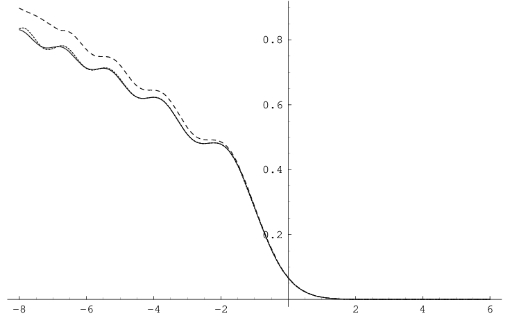
2^{-\frac{1}{2}}n^{-\frac{1}{6}}\rho_{n}(x)=2^{-\frac{1}{2}}n^{-\frac{1}{6}}K_{n}(x,x)=[\airy^{{}^{\prime}}(X)]^{2}-X[\airy(X)]^{2}-c_{G}\,[\airy(X)]^{2}n^{-\frac{1}{3}}+

\frac{1}{20}\left\{2X[\airy^{{}^{\prime}}(X)]^{2}-3X^{2}[\airy(X)]^{2}+(3-20c_{G}^{2})\airy^{{}^{\prime}}(X)\airy(X)\right\}n^{-\frac{2}{3}}+O(n^{-1})F_{n}(X)

(3.16)

Note that for $c_{G}=0$ , this is formula (72) of [7]. Figure 3.3.1 illustrates the accuracy of equation (3.16).

Refer to caption — Figure 3.3.1: For $c_{G}=0$ and $n=40$ , The dashed curve is the usual approximation of the one point correlation function from the Airy kernel (which is the first two terms in (3.16)), the solid curve is the exact scaled one point correlation function and the doted curve is our approximation (3.16)

For the Laguerre case,

Theorem 3.5.

For $\;x=4(n+1)+2\alpha+4c_{L}+2(2(n+1))^{\frac{1}{3}}X\quad$ and
$y=4(n+1)+2\alpha+4c_{L}+2(2(n+1))^{\frac{1}{3}}Y\;$ with $\;X,c_{L}$ and $\;Y\;$ bounded,

\displaystyle K_{n+1}^{\alpha}(x,y)\,dx=\left\{K_{\airy}(X,Y)-2^{\frac{2}{3}}c_{L}\airy(X)\airy(Y)(n+1)^{-\frac{1}{3}}+\right.

\displaystyle\frac{2^{\frac{1}{3}}}{10}\left[\quad(X^{2}+XY+Y^{2})\airy(X)\airy(Y)-(X+Y)\airy^{{}^{\prime}}(X)\airy^{{}^{\prime}}(Y)-\right.

\left.\left.(10c_{L}^{2}-1)(\airy(X)\airy^{{}^{\prime}}(Y)+\airy^{{}^{\prime}}(X)\airy(Y))\right](n+1)^{-\frac{2}{3}}+O((n+1)^{-1})F(X,Y)\right\}\,dX

(3.17)

The error term $F(X,Y)$ is again the kernel of an integral operator on $L^{2}(J)$ which is trace class for any subset $J$ of the reals which is bounded away from minus infinity.

Taking the limit as $y$ goes to $x$ in (3.17) gives the one point correlation function $\rho_{n+1}^{\alpha}$ in the Laguerre case.

Corollary 3.6.

For $x=4(n+c_{L})+2\alpha+2(2n)^{\frac{1}{3}}X\,,$

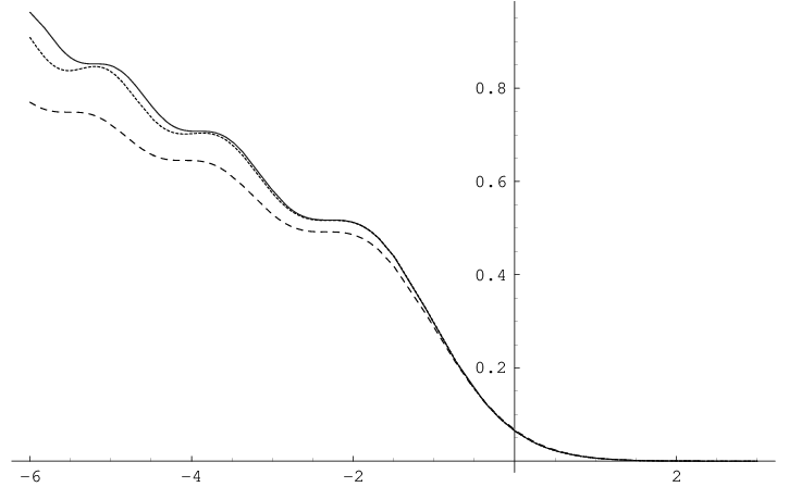
2(2n)^{\frac{1}{3}}\rho_{n}^{\alpha}(x)=[\airy^{{}^{\prime}}(X)]^{2}-X[\airy(X)]^{2}-2^{\frac{2}{3}}\,c_{L}[\airy(X)]^{2}n^{-\frac{1}{3}}+

\frac{2^{\frac{1}{3}}}{10}[3X^{2}[\airy(X)]^{2}-2X[\airy^{{}^{\prime}}(X)]^{2}+2(1-10\,c_{L}^{2})\airy(X)\airy^{{}^{\prime}}(X)]n^{-\frac{2}{3}}+O(n^{-1})F(X)

(3.18)

Note that for $\;c_{L}=-\alpha/2\;$ this is formula (73) in [7]. Figure 3.3.2 illustrates the accuracy of our result. Combining Lemma 3.1, Lemma 3.2 and the fine-tuned constants in (3.14) give Theorem 1.4.

Appendix A Proof of Theorem1.1

In this section we will follow Szegö [18], Section 8.75. With the following changes.

•

We introduce a new variable $\;c\;$ in the definition of $\;l_{n}\;$ to fine-tune the final result. $\;l_{n}=(4n+2\alpha+2c)^{\frac{1}{2}}\;$ instead of $\;l_{n}=(4n+2\alpha+2)^{\frac{1}{2}}$ .
•

We will use the second order Hankel expansion of the Bessel function of large argument instead of the first order.
•

We define $\;\xi=l_{n}+(2l_{n})^{-\frac{1}{3}}t\;$ instead of $\;\xi=l_{n}-(6l_{n})^{-\frac{1}{3}}t\;$ to match the definition of the Airy function with the one commonly used.
•

We give an estimate of the error term as a function of the independent variable

recalling the generating function of the Laguerre polynomials.

\sum_{n=0}^{\infty}\frac{L_{n}^{\alpha}(x)}{\Gamma(n+\alpha+1)}\omega^{n}=e^{\omega}(x\omega)^{-\frac{\alpha}{2}}J_{\alpha}(2(x\omega)^{\frac{1}{2}})

(A.1)

The substitutions $x\rightarrow\xi$ and $\omega\rightarrow-\frac{\omega^{2}}{4}$ , and for edge scaling $l_{n}=(4n+2\alpha+2c)^{\frac{1}{2}}$ , $\omega\rightarrow l_{n}z.\;$ we deduce from (A.1)

\frac{L_{n}^{\alpha}(\xi^{2})}{\Gamma(n+\alpha+1)}(-\frac{1}{4})^{n}=\frac{2^{\alpha}(\xi)^{-\alpha}}{2\pi i}l_{n}^{-2n-\alpha}\int_{\gamma}e^{-\frac{l_{n}^{2}z^{2}}{4}-\frac{1}{2}l_{n}^{2}log(z)}z^{c-1}e^{\frac{\pi\alpha i}{2}}J_{\alpha}(e^{-\frac{\pi i}{2}}\xi l_{n}z)dz\quad

(A.2)

where $\gamma$ is a symmetric contour enclosing the origin.

Using the Hankel expansion of the Bessel function of large argument (see, for example, Olver [15, pgs 130–132] ): that⁷⁷ 7 In the following formula the $O$ -term is actually of the form $O(\frac{1}{|\xi l_{n}z|^{2}})e^{\xi l_{n}z}+O(\frac{1}{|\xi l_{n}z|^{2}})e^{-\xi l_{n}z+(\alpha+\frac{1}{2})\pi i}.$ as $|l_{n}z|\rightarrow\infty$ in $|\arg(z)|\leq\pi-\delta(<\pi)$ ,

	$\displaystyle e^{\frac{\pi\alpha i}{2}}J_{\alpha}(e^{-\frac{\pi i}{2}}\xi l_{n}z)$	$\displaystyle=$	$\displaystyle(2\pi\xi l_{n})^{-\frac{1}{2}}z^{-\frac{1}{2}}\left[e^{\xi l_{n}z}+e^{-\xi l_{n}z+(\alpha+\frac{1}{2})\pi i}\right.$
		$\displaystyle+$	$\displaystyle\left.\frac{4\alpha^{2}-1}{8\xi l_{n}z}(-e^{\xi l_{n}z}+e^{-\xi l_{n}z+(\alpha+\frac{1}{2})\pi i})+O(\frac{1}{\|\xi l_{n}z\|^{2}})\right]$

Substituting this in (A.2) for $\xi=l_{n}+(2l_{n})^{-\frac{1}{3}}t\;$ with $t$ bounded,

\frac{L_{n}^{\alpha}(\xi^{2})}{\Gamma(n+\alpha+1)}(-\frac{1}{4})^{n}=\frac{2^{\alpha}(l_{n}+(2l_{n})^{-\frac{1}{3}}t)^{-\alpha}}{2\pi i}l_{n}^{-2n-\alpha}(2\pi(l_{n}+(2l_{n})^{-\frac{1}{3}}t)l_{n})^{-\frac{1}{2}}\cdot

\left\{\int_{\gamma}(1-\frac{4\alpha^{2}-1}{8l_{n}^{2}z(1+2^{-\frac{1}{3}}l_{n}^{-\frac{4}{3}}t)})e^{-\frac{l_{n}^{2}z^{2}}{4}-\frac{1}{2}l_{n}^{2}\log(z)+l_{n}^{2}z+2^{-\frac{1}{3}}l_{n}^{-\frac{1}{3}}l_{n}zt}\quad z^{c-\frac{3}{2}}dz\quad+\right.

e^{(\alpha+\frac{1}{2})\pi i}\int_{\gamma}(1+\frac{4\alpha^{2}-1}{8l_{n}^{2}z(1+2^{-\frac{1}{3}}l_{n}^{-\frac{4}{3}}t)})e^{-\frac{l_{n}^{2}z^{2}}{4}-\frac{1}{2}l_{n}^{2}\log(z)-l_{n}^{2}z-2^{-\frac{1}{3}}l_{n}^{-\frac{1}{3}}l_{n}zt}\quad z^{c-\frac{3}{2}}dz

+\left.0(l_{n}^{-4})\int_{\gamma}|e^{-\frac{l_{n}^{2}z^{2}}{4}-\frac{1}{2}l_{n}^{2}\log(z)\pm l_{n}^{2}z\pm 2^{-\frac{1}{3}}l_{n}^{-\frac{1}{3}}l_{n}zt}|\quad|dz|\quad\quad\right\}

(A.3)

The $\pm$ signs would be taken according to which one gives the larger contribution. To simplify notations we set $p=(4\alpha^{2}-1)/(8l_{n}^{2}z(1+2^{-\frac{1}{3}}l_{n}^{-\frac{4}{3}}t))$ .

The integral over $\gamma$ can be split into the path in the upper half-plane and the path in the lower half-plane. However the lower-half plane part of the path can be transformed into the upper half plane via the transformation $z\rightarrow\bar{z}$ , taking into account the orientation change and the fact that the integrand is an analytic function of $z$ on $\gamma$ . The integrand will be transformed into its complex conjugate under this transformation. The Jacobian of the transformation is $-1$ so it will reverse the orientation once again. Thus the lower half plane contribution of the integral is equal to the conjugate of the upper half contribution such that the integral over $\gamma$ is exactly twice the real part of the integral over the upper half portion $\gamma_{+}$ of the contour. Thus (A.3) is equal to

2^{\alpha}(l_{n}+(2l_{n})^{-\frac{1}{3}}t)^{-\alpha}l_{n}^{-2n-\alpha}(2\pi(l_{n}+(2l_{n})^{-\frac{1}{3}}t)l_{n})^{-\frac{1}{2}}\cdot 2\mathcal{R}e\{\frac{1}{2\pi i}G+\frac{1}{2\pi i}H+K\}

(A.4)

where

G=\int_{\gamma_{+}}(1-p)e^{-l_{n}^{2}f_{1}(z)+2^{-\frac{1}{3}}l_{n}^{\frac{2}{3}}z\,t}\,z^{c-\frac{3}{2}}\,dz=\int_{\gamma_{+}}e^{-l_{n}^{2}f_{1}(z)}g(z)\,dz

(A.5)

\textrm{with}\quad f_{1}(z)=\frac{z^{2}}{4}-z+\frac{1}{2}\log(z)

H=e^{(\alpha+\frac{1}{2})\pi i}\int_{\gamma_{+}}(1+p)e^{-l_{n}^{2}f_{2}(z)-2^{-\frac{1}{3}}l_{n}^{\frac{2}{3}}zt}\,z^{c-\frac{3}{2}}\,dz=\int_{\gamma_{+}}e^{-l_{n}^{2}f_{2}(z)}h(z)\,dz

(A.6)

\textrm{with}\quad f_{2}(z)=\frac{z^{2}}{4}+z+\frac{1}{2}\log(z)

\textrm{and}\quad K=0(l_{n}^{-4})\int_{\gamma_{+}}|e^{-\frac{l_{n}^{2}z^{2}}{4}-\frac{1}{2}l_{n}^{2}log(z)\pm l_{n}^{2}z\pm 2^{-\frac{1}{3}}l_{n}^{\frac{2}{3}}zt}|\quad|dz|

(A.7)

We will use the steepest descent method to find an asymptotic expansion for $G,H$ and $K$ for large $l_{n}$ keeping $\alpha$ fixe and $c$ bounded.⁸⁸ 8 Actually $c$ can grow with $n$ , but we are not going to look at this problem.

A.1 Steepest descent method for G

The steepest descent for this section is with respect to large $l_{n}$ in (A.5). The saddle point condition $f^{{}^{\prime}}(z)=0$ gives $z_{0}=1$ with $f^{{}^{\prime\prime}}(1)=0$ .

The steepest descent curve leaves $z_{0}=1$ at angles $0,\ \pi/3,\$ or $\ 2\pi/3$ . The direction of maximum decreases of $f_{1}$ is $\ 2\pi/3$ . We deform $\gamma_{+}$ at $z_{0}=1$ such that the resulting contour leaves $z_{0}=1$ at angle $2\pi/3\;$ as the line segment

z=1+2^{\frac{1}{3}}l_{n}^{-\frac{2}{3}}\rho e^{\frac{2\pi i}{3}}\quad\textrm{ with }0\leq\rho\leq n^{\delta}\quad\textrm{ where }\quad 0<\delta<\frac{1}{6}

(A.8)

then along the segment symmetric to this segment with respect to the imaginary axis and finally connect the tip of these two line segments by an arc of circle centered at the origin with radius $r$ . For simplicity, we will also call this path⁹⁹ 9 See [18, Section 8.75] for an illustration of this path. $\gamma_{+}$ .

In the following sections, we will estimate the contribution of each portion of the contour to $G$ .

A.1.1 On the arc of circle $z=re^{\phi i}$

Since $\mathcal{R}e(-f_{1}(z))=-\frac{1}{4}r^{2}\cos 2\phi+r\cos\phi-\frac{1}{2}\log(r)$ is a decreasing function of $\phi$ for $0<\phi<\pi$ , the major contribution of this arc is bounded above by the value of the integrand at the end point where $\rho=n^{\delta}$ . A deformation of the path of integration near $-1$ is immaterial so the estimate of the remainder of the path is again bounded above by the value of the integrand at $\rho=n^{\delta}$ . (Therefore in the next section we will focus on the asymptotics on the line segment in the first quadrant only.)

If we set $\;z=re^{i\theta}\;$ where $\;r^{2}=1+2^{\frac{2}{3}}l_{n}^{-\frac{4}{3}}n^{2\delta}-2^{\frac{1}{3}}l_{n}^{-\frac{2}{3}}n^{\delta}\;$ and $\;\theta_{0}\leq\theta\leq\pi-\theta_{0}\;$ where $\;\theta_{0}\;$ is the angle that the ray from the origin to the tip of the line segment makes with the real axis, $\;\cos(\theta_{0})=\frac{2-2^{\frac{1}{3}}l_{n}^{-\frac{2}{3}}n^{\delta}}{2r}.$ The modulus of this integrand in (A.5) is of order

r^{c-\frac{3}{2}}e^{k(\theta)}\quad\textrm{where}\quad k(\theta)=-\frac{1}{4}r^{2}\,\cos(2\theta)+r\,\cos(\theta)-\frac{1}{2}\log(r)+2^{-\frac{1}{3}}l_{n}^{-\frac{4}{3}}\,r\,t\cos(\theta)

$k^{{}^{\prime}}$ has roots $\;\pi,\;0\;$ and $\;\theta_{2}\;\textrm{where}\;\cos(\theta_{2})=\frac{1+2^{-\frac{1}{3}}l_{n}^{-\frac{4}{3}}t}{r}\;$ , for large $\;l_{n}$ , $\;0\leq\theta_{2}\leq\theta_{0}\;$ . $k$ increases from $0$ to $\theta_{2}$ and decreases from $\theta_{2}$ to $\pi$ . Therefore the maximum of $k(\theta)$ on the arc of circle is at $\theta_{0}$ . We can also use this as an upper bound of the contribution of the contour around $-1$ . Thus the contribution of the arc of circle and the line segment on the second quadrant is of order of the modulus of the integrand evaluated at the tip of the line segment in the first quadrant.We can therefore focus our attention in the next section on just the line segment in the first quadrant. The parametrization (A.8) shows that $\rho$ will go to infinity with $n$ , so we want to estimate the contribution not only of the line segment but of the whole ray $\;0\leq\rho\leq\infty\;$ . The error that we make by taking the ray is $\;|\int_{n^{\delta}}^{\infty}z^{c-\frac{2}{3}}e^{-l_{n}^{2}f_{1}(z)+2^{-\frac{1}{3}}l_{n}^{\frac{2}{3}}tz}dz|$ .
On the ray, $\;-l_{n}^{2}f_{1}(z)=\frac{3}{4}l_{n}^{2}-\frac{\rho^{3}}{3}+O(\rho^{4})l_{n}^{-\frac{2}{3}}\;$ , thus
$\int_{n^{\delta}}^{\infty}z^{c-\frac{2}{3}}e^{-l_{n}^{2}f_{1}(z)+2^{-\frac{1}{3}}l_{n}^{\frac{2}{3}}tz}dz=O(1)2^{\frac{1}{3}}l_{n}^{-\frac{2}{3}}e^{\frac{3}{4}l_{n}^{2}+2^{-\frac{1}{3}}l_{n}^{\frac{2}{3}}t}\int_{n^{\delta}}^{\infty}e^{-\frac{\rho^{3}}{3}+\rho te^{\frac{2\pi i}{3}}}d\rho$ .
We therefore need to give an estimate an estimate of the integral on the right of this last equality and an estimate of the integrand when $\;\rho=n^{\delta}$ in (A.5).

Integrand when $\;\rho=n^{\delta}$
The order of the integrand for large $n$ is $\quad O(1)2^{\frac{1}{3}}l_{n}^{-\frac{2}{3}}e^{\frac{3}{4}l_{n}^{2}+2^{-\frac{1}{3}}l_{n}^{\frac{2}{3}}t}\,e^{-\frac{\rho^{3}}{3}+\rho te^{\frac{2\pi i}{3}}}.$
We need to give an estimate of the factor $\;u:=e^{-\frac{\rho^{3}}{3}+\rho te^{\frac{2\pi i}{3}}}\;$ as a function of $\;t$ .
If $t$ is positive, it is of order $e^{-\frac{n^{3\delta}}{3}}\cdot e^{-\frac{tn^{\delta}}{2}}$ or of order $e^{-\frac{n^{3\delta}}{3}}\cdot e^{-t}.$
If $t$ is negative, we have $\;|u|=e^{-\frac{\rho^{3}}{3}+\frac{\rho y}{2}}$ where $y=-t$ . For trace class convergence we need an estimate that will decay exponentially for large $t$ . The expansion of the exponent in $|u|$ around his critical point $\rho_{0}=-\sqrt{\frac{y}{2}}$ is $-\frac{2}{3}(\frac{y}{2})^{\frac{3}{2}}+\sqrt{\frac{y}{2}}(\rho+\sqrt{\frac{y}{2}})^{2}-\frac{1}{3}(\rho+\sqrt{\frac{y}{2}})^{3}$ . Thus for $\rho=n^{\delta},\;u$ is of order $e^{-\frac{(n^{\delta}+\sqrt{\frac{y}{2}})^{3}}{3}}\cdot e^{-\frac{2}{3}(\frac{y}{2})^{\frac{3}{2}}}$ or of order $e^{-\frac{n^{3\delta}}{3}}\cdot e^{-y}$ since $y$ is bounded and positive. So in either case the contribution is of order, $e^{-\frac{n^{3\delta}}{3}}\cdot e^{-|t|}$ .

Tail integration
We show that the contribution of $\int_{n^{\delta}}^{\infty}e^{-\frac{\rho^{3}}{3}-\frac{\rho t}{2}}d\rho\quad$ is of the same order.

If $\;t\geq 0\,,$ $\quad\int_{n^{\delta}}^{\infty}e^{-\frac{\rho^{3}}{3}-\frac{\rho t}{2}}d\rho\,\leq\int_{n^{\delta}}^{\infty}e^{-\frac{\rho^{3}}{3}-\frac{t}{2}}d\rho\,=e^{-\frac{t}{2}}\int_{n^{\delta}}^{\infty}e^{-\frac{\rho^{3}}{3}}d\rho\,\leq e^{-\frac{t}{2}}\int_{n^{\delta}}^{\infty}e^{-\frac{\rho}{3}}d\rho$
so it is of order $e^{-\frac{n^{\delta}}{3}}\cdot e^{-\frac{t}{2}}$
If $t$ is negative, a similar change of variable and expansion of the integrand leads to
$\int_{n^{\delta}}^{\infty}e^{-\frac{\rho^{3}}{3}-\frac{\rho t}{2}}d\rho\quad=\int_{n^{\delta}}^{\infty}e^{-\frac{2}{3}(\frac{y}{2})^{\frac{3}{2}}+\sqrt{\frac{y}{2}}(\rho+\sqrt{\frac{y}{2}})^{2}-\frac{1}{3}(\rho+\sqrt{\frac{y}{2}})^{3}}d\rho$
$e^{-\frac{2}{3}(\frac{y}{2})^{\frac{3}{2}}}\int_{n^{\delta}}^{\infty}e^{-\frac{1}{3}(\rho+\sqrt{\frac{y}{2}})^{3}[1-3(\rho+\sqrt{\frac{y}{2}})^{-1}\sqrt{\frac{y}{2}}]}d\rho\quad\sim e^{-\frac{2}{3}(\frac{y}{2})^{\frac{3}{2}}}\int_{n^{\delta}}^{\infty}e^{-\frac{1}{3}(\rho+\sqrt{\frac{y}{2}})^{3}}d\rho$
This is of order, $e^{-\frac{2}{3}(\frac{y}{2})^{\frac{3}{2}}}\int_{n^{\delta}}^{\infty}e^{-\frac{1}{3}(\rho+\sqrt{\frac{y}{2}})}d\rho$ or of order $e^{-\frac{2}{3}(\frac{y}{2})^{\frac{3}{2}}}\cdot e^{-\frac{1}{3}(n^{\delta}+\sqrt{\frac{y}{2}})}$
So the contribution of this integral is of order $e^{-\frac{n^{\delta}}{3}}\cdot e^{-|t|}$

We conclude this subsection by recording that the error that we make by neglecting the remainder of the contour and considering the integral from zero to infinity instead of zero to $n^{\delta}$ is at most of order

2^{\frac{1}{3}}l_{n}^{-\frac{2}{3}}e^{\frac{3}{4}l_{n}^{2}+2^{-\frac{1}{3}}l_{n}^{\frac{2}{3}}t}e^{-\frac{n^{\delta}}{3}}\cdot e^{-|t|}

(A.9)

A.1.2 On the ray $z=1+2^{\frac{1}{3}}l_{n}^{-\frac{2}{3}}\rho e^{\frac{2\pi i}{3}},\quad\rho\in[0,\infty)$

The Taylor expansion of $f_{1}$ at $z_{0}=1$ is
$\quad f_{1}(z)=-\frac{3}{4}+\frac{\rho^{3}}{3}l_{n}^{-2}-\frac{1}{2}\sum_{k=4}^{\infty}c_{1,k}(\rho l_{n}^{-\frac{2}{3}})^{k}\quad$ with $\;c_{1,k}=(-1)^{k}\frac{2^{\frac{k}{3}}e^{\frac{2\pi ki}{3}}}{k}$ , and

$\quad 2^{-\frac{1}{3}}l_{n}^{\frac{2}{3}}tz=2^{-\frac{1}{3}}l_{n}^{\frac{2}{3}}t+\rho te^{\frac{2\pi i}{2}}.\quad$ Taking in account the error estimate from (A.9), the substitution of these quantities in $G$ give,

G=2^{\frac{1}{3}}l_{n}^{-\frac{2}{3}}e^{\frac{2\pi i}{3}}e^{\frac{3}{4}l_{n}^{2}+2^{-\frac{1}{3}}l_{n}^{\frac{2}{3}}t}\cdot\left\{\int_{0}^{\infty}e^{-\frac{\rho^{3}}{3}+\rho te^{\frac{2\pi i}{3}}}g_{n}(\rho)\,d\rho\quad+O(e^{-\frac{n^{\delta}}{3}})\cdot e^{-|t|}\right\}\quad\textrm{ with}

g_{n}(\rho)=(1-\frac{4\alpha^{2}-1}{8l_{n}^{2}(1+2^{\frac{1}{3}}l_{n}^{-\frac{2}{3}}\rho e^{\frac{2\pi i}{3}})(1+2^{-\frac{1}{3}}l_{n}^{-\frac{4}{3}}t)})(1+2^{\frac{1}{3}}l_{n}^{-\frac{2}{3}}\rho e^{\frac{2\pi i}{3}})^{c-\frac{3}{2}}e^{\frac{1}{2}\sum_{k=4}^{\infty}c_{1,k}(\rho l_{n}^{-\frac{2}{3}})^{k}l_{n}^{2}}

(A.10)

A.2 Steepest descent for H

The analysis for $H$ differs from that of $G$ in the location of the saddle point, and the orientation of the contour. A similar analysis shows that the saddle point is now at $z_{0}=-1$ , the final contour of integration is the same but oriented in the opposite direction. It leaves $z_{0}$ at angle $\pi/3$ . The error estimate on the arc of circle and on the tail of the corresponding ray is the same. The new parametrization on the ray is $\;z=-1+2^{\frac{1}{3}}l_{n}^{-\frac{2}{3}}e^{\frac{\pi i}{3}}\rho=-(1+2^{\frac{1}{3}}l_{n}^{-\frac{2}{3}}e^{-\frac{2\pi i}{3}}\rho),\quad 0\leq\rho\leq\infty$
The Taylor expansion of $f_{2}$ at $z=-1$ is

f_{2}(z)=-\frac{3}{4}+\frac{\pi}{2}i+l_{n}^{-2}\frac{\rho^{3}}{3}-\frac{1}{2}\sum_{k\geq 4}c_{2,k}\rho^{k}l_{n}^{-\frac{2k}{3}},\quad\textrm{with}\quad c_{2,k}=(-1)^{k}\frac{2^{\frac{k}{3}}e^{-\frac{2\pi ki}{3}}}{k}

This leads to

H=-2^{\frac{1}{3}}l_{n}^{-\frac{2}{3}}e^{-\frac{2\pi i}{3}}e^{\frac{3}{4}l_{n}^{2}+2^{-\frac{1}{3}}l_{n}^{\frac{2}{3}}t}\cdot\left\{\int_{0}^{\infty}e^{-\frac{\rho^{3}}{3}+\rho te^{-\frac{2\pi i}{3}}}h_{n}(\rho)\,d\rho\quad+O(e^{-\frac{n^{\delta}}{3}})\cdot e^{-|t|}\right\}\quad\textrm{ with}

h_{n}(\rho)=(1-\frac{4\alpha^{2}-1}{8l_{n}^{2}(1+2^{\frac{1}{3}}l_{n}^{-\frac{2}{3}}\rho e^{-\frac{2\pi i}{3}})(1+2^{-\frac{1}{3}}l_{n}^{-\frac{4}{3}}t)})(1+2^{\frac{1}{3}}l_{n}^{-\frac{2}{3}}\rho e^{-\frac{2\pi i}{3}})^{c-\frac{3}{2}}e^{\frac{1}{2}\sum_{k=4}^{\infty}c_{2,k}(\rho l_{n}^{-\frac{2}{3}})^{k}l_{n}^{2}}

(A.11)

A.3 Asymptotics for K

The asymptotics of the integral factor in K depends on the leading term in the expansion of either G or H, depending on which one is larger as shown in (A.7). But from the previous analysis, the leading term of both G and H are of the same order. Thus K is also of order of a nonzero linear combination of the leading terms in G and in H times $O(l_{n}^{-4})$ . In our case¹⁰¹⁰ 10 The choice of this representation of the error is for trace class convergence of the final result. we take the linear combination to be $\quad\mathcal{R}e\frac{1}{2\pi i}(\textbf{G}+\textbf{H})$ .

A.4 Conclusion

Note that from (A.10) and (A.11) we see that except for the $O$ -term, $H=-\overline{G}$ .
The change of variable $\;\rho\mapsto\rho e^{-\frac{2\pi i}{3}}\;$ transform $g_{n}(\rho)$ into a real function $g_{1}(\rho)$ and

\displaystyle\textbf{G}=2^{\frac{1}{3}}l_{n}^{-\frac{2}{3}}e^{\frac{3}{4}l_{n}^{2}+2^{-\frac{1}{3}}l_{n}^{\frac{2}{3}}t}\cdot(\int_{0}^{\infty e^{\frac{2\pi i}{3}}}e^{(-\frac{\rho^{3}}{3}+\rho t)}g_{1}(\rho)d\rho+O(e^{-\frac{n^{\delta}}{3}})e^{-|t|}),\quad\textrm{note also that}

2\mathcal{R}e\frac{1}{2\pi i}(G+H)=2\cdot 2^{\frac{1}{3}}l_{n}^{-\frac{2}{3}}e^{\frac{3}{4}l_{n}^{2}+2^{-\frac{1}{3}}l_{n}^{\frac{2}{3}}t}\cdot

\left\{\frac{1}{2\pi i}[\int_{\infty e^{-\frac{2\pi i}{3}}}^{0}e^{(-\frac{\rho^{3}}{3}+\rho t)}g_{1}(\rho)d\rho+\int_{0}^{\infty e^{\frac{2\pi i}{3}}}e^{(-\frac{\rho^{3}}{3}+\rho t)}g_{1}(\rho)d\rho]+O(e^{-\frac{n^{\delta}}{3}})e^{-|t|}\right\}

(A.12)

At this point we can give an estimate for K based on this last formula since the leading term of $g_{1}$ is 1.

\textbf{K}=O(l_{n}^{4})\cdot 2^{\frac{1}{3}}l_{n}^{-\frac{2}{3}}e^{\frac{3}{4}l_{n}^{2}+2^{-\frac{1}{3}}l_{n}^{\frac{2}{3}}t}\cdot\frac{1}{2\pi i}(\int_{\infty e^{-\frac{2\pi i}{3}}}^{0}e^{(-\frac{\rho^{3}}{3}+\rho t)}d\rho+\int_{0}^{\infty e^{\frac{2\pi i}{3}}}e^{(-\frac{\rho^{3}}{3}+\rho t)}d\rho)

=\quad O(l_{n}^{-4})\cdot 2^{\frac{1}{3}}l_{n}^{-\frac{2}{3}}e^{\frac{3}{4}l_{n}^{2}+2^{-\frac{1}{3}}l_{n}^{\frac{2}{3}}t}\cdot\airy(t)

(A.13)

\textrm{where}\quad\airy(t)=\frac{1}{2\pi i}(\int_{\infty e^{-\frac{2\pi i}{3}}}^{0}e^{(-\frac{\rho^{3}}{3}+\rho t)}d\rho+\int_{0}^{\infty e^{\frac{2\pi i}{3}}}e^{(-\frac{\rho^{3}}{3}+\rho t)}d\rho)\quad\textrm{is the Airy function}

(A.14)

To simplify notation, we will combine the two paths of integration in G and call the new path $\sigma$ .

With this notation, (A.4) gives

e^{-\frac{\xi^{2}}{2}}L_{n}^{\alpha}(\xi^{2})=(-1)^{n}2^{2n}\Gamma(n+\alpha+1)2^{\alpha}(\xi)^{-\alpha}e^{-\frac{\xi^{2}}{2}}l_{n}^{-2n-\alpha}(2\pi\xi l_{n})^{-\frac{1}{2}}2\cdot 2^{\frac{1}{3}}l_{n}^{-\frac{2}{3}}e^{\frac{3}{4}l_{n}^{2}+2^{-\frac{1}{3}}l_{n}^{\frac{2}{3}}t}\cdot

[\frac{1}{2\pi i}\int_{\sigma}e^{(-\frac{\rho^{3}}{3}+\rho t)}g_{1}(\rho)d\rho\quad+\quad O(l_{n}^{-4})Ai(t)\quad+\quad O(e^{-\frac{n^{\delta}}{3}})e^{-|t|}]

(A.15)

Using (A.10) and the help of Mathematica, we have the following expansion¹¹¹¹ 11 The expansion is valid for this derivation up to $l_{n}^{-6\frac{2}{3}}$ as the error estimate for $K$ indicates. We choose to stop here at $l_{n}^{-4\frac{2}{3}}$ note also that the last term will served to estimate the error. of $g_{1}$ in powers of $l_{n}^{-\frac{2}{3}}$ .

1\;+\;2^{\frac{1}{3}}(\frac{{\rho}^{4}}{4}+(c-\frac{3}{2})\rho)\;l_{n}^{-\frac{2}{3}}\;+2^{\frac{2}{3}}\left(-\frac{{\rho}^{5}}{5}+\frac{{\rho}^{8}}{32}+\frac{(c-\frac{3}{2}){\rho}^{5}}{4}+\frac{(c-\frac{3}{2}){\rho}^{2}(c-\frac{5}{2})}{2}\right)\;l_{n}^{-\frac{4}{3}}

+\left(\frac{(c-\frac{3}{2}){\rho}^{6}(c-\frac{5}{2})}{4}+\frac{\rho^{6}}{3}-\frac{\rho^{9}}{10}+\frac{{\rho}^{12}}{192}+\frac{1}{3}(c-\frac{3}{2}){\rho}^{3}(c-\frac{5}{2})(c-\frac{7}{2})\quad-\right.

\left.\frac{a^{2}}{2}+\frac{1}{8}+(c-\frac{3}{2})2\rho(-\frac{{\rho}^{5}}{5}+\frac{{\rho}^{8}}{32})\right)l_{n}^{-2}\quad+

\left(2^{\frac{1}{3}}(-\frac{2{\rho}^{7}}{7}+\frac{{\rho}^{10}}{12}+\frac{{\rho}^{10}}{25}-\frac{{\rho}^{13}}{80}+\frac{{\rho}^{16}}{3072})+\frac{1}{4}\left(\frac{(c-\frac{3}{2}){\rho}^{3}(c-\frac{5}{2})(c-\frac{7}{2})}{3}-\frac{a^{2}}{2}+\frac{1}{8}\right)\sqrt[3]{2}{\rho}^{4}\right.

+(c-\frac{3}{2}){2}^{\frac{1}{3}}{\rho}^{2}(c-\frac{5}{2})(-\frac{{\rho}^{5}}{5}+\frac{{\rho}^{8}}{32})+(c-\frac{3}{2})2^{\frac{1}{3}}\rho(\frac{{\rho}^{6}}{3}-\frac{\rho^{9}}{10}+\frac{\rho^{12}}{192})

\left.+\frac{2^{\frac{1}{3}}}{12}(c-\frac{3}{2}){\rho}^{4}(c-\frac{5}{2})(c-\frac{7}{2})(c-\frac{9}{2})+(-\frac{a^{2}}{2}+\frac{1}{8})(c-\frac{3}{2})2^{\frac{1}{3}}\rho-\frac{1}{8}(-4\,{a}^{2}+1)2^{\frac{1}{3}}\rho\right)l_{n}^{-8/3}

+q(\rho)O(l_{n}^{-\frac{10}{3}})\quad\textrm{for some polynomial}\;q

The integral in (A.15) can be expresses as a linear combination of the Airy function and its derivative using $\;\airy^{(k)}(t)=\frac{1}{2\pi i}\int_{\sigma}e^{-\frac{\rho^{3}}{3}+\rho t}\rho^{k}d\rho\;$ and this expansion of $\;g_{1}$ . Using the Airy differential equation $\airy^{\prime\prime}(t)=t\airy(t)$ , it reduces to an expression involving only the independent variable $t$ , $\airy$ and $\airy^{\prime}$ .
The contribution of the last term of the expansion of $g_{1}$ is a finite combination of the form $\;\sum_{m=0}^{k}(p_{m}(t)\,\airy(t)+q_{m}(t)\,\airy^{\prime}(t))\;$ for some polynomials $p$ and $q$ . If $t$ is bounded away from minus infinity, this is of order $\airy(t)$ . In this paper we assume therefore that this is the case for $t$ .
If $\;\xi=l_{n}+(2l_{n})^{-\frac{1}{3}}t\;$ we have
$e^{-\frac{\xi^{2}}{2}}\xi^{-(\alpha+\frac{1}{2})}=l_{n}^{-(\alpha+\frac{1}{2})}e^{-\frac{l_{n}^{2}}{2}-2^{-\frac{1}{3}}l_{n}^{\frac{2}{3}}t}[1-\frac{t^{2}}{2^{2}}2^{\frac{1}{3}}l_{n}^{-\frac{2}{3}}+(\frac{t^{4}}{2^{5}}-(2\alpha+1)\frac{t}{2^{2}})2^{\frac{2}{3}}l_{n}^{-\frac{4}{3}}+(-\frac{t^{6}}{3\cdot 2^{6}}+(2\alpha+1)\frac{t^{3}}{2^{3}})l_{n}^{-2}+O(l_{n}^{-\frac{8}{3}}t^{2})]$ .
Stirling formula gives $\;\Gamma(n+\alpha+1)=2^{\frac{1}{2}}\pi^{\frac{1}{2}}n^{n+\alpha+\frac{1}{2}}e^{-n}[1+\frac{6\alpha(\alpha+1)+1}{12n}+O(n^{-2})]\quad$ and we have $l_{n}^{-2n-2\alpha-\frac{5}{3}}=2^{-2n-2\alpha-\frac{5}{3}}n^{-n-\alpha-\frac{5}{6}}e^{-\frac{\alpha+c}{2}}[1+\frac{(\alpha+c)(-9\alpha+3c-10)}{24n}+O(n^{-2})]$ .

Thus
$(-1)^{n}2^{2n}\Gamma(n+\alpha+1)2^{\alpha}(\xi)^{-\alpha}l_{n}^{-2n-\alpha}(2\pi\xi l_{n})^{-\frac{1}{2}}2\cdot 2^{\frac{1}{3}}l_{n}^{-\frac{2}{3}}e^{\frac{3}{4}l_{n}^{2}+2^{-\frac{1}{3}}l_{n}^{\frac{2}{3}}t}e^{-\frac{\xi^{2}}{2}}=\\ \\ (-1)^{n}2^{-\alpha-\frac{1}{3}}n^{-\frac{1}{3}}(1+\frac{3\alpha^{2}+2\alpha-6\alpha c+3c^{2}-10c+2}{24n}+O(n^{-2}))[1-\frac{t^{2}}{2^{2}}2^{\frac{1}{3}}l_{n}^{-\frac{2}{3}}+(\frac{t^{4}}{2^{5}}-(2\alpha+1)\frac{t}{2^{2}})2^{\frac{2}{3}}l_{n}^{-\frac{4}{3}}+(-\frac{t^{6}}{3\cdot 2^{6}}+(2\alpha+1)\frac{t^{3}}{2^{3}})l_{n}^{-2}+O(l_{n}^{-\frac{8}{3}}t^{2})]$ .

This in (A.15) together with the expansion of $g_{1}$ give the desired result.¹²¹² 12 Actually $\xi=(4n+2\alpha+2c)^{\frac{1}{2}}+\frac{t}{2^{\frac{2}{3}}n^{\frac{1}{6}}}+O(n^{-\frac{7}{6}}),$ but due to the smoothness of $\;e^{-\frac{\xi^{2}}{2}}L_{n}^{\alpha}(\xi^{2})$ the error that we make by removing the $O$ -term is negligible if we are aiming for an accuracy of order $n^{-1}$ .

For $\xi=(4n+2\alpha+2c)^{\frac{1}{2}}+\frac{t}{2^{\frac{2}{3}}n^{\frac{1}{6}}}\quad$ and $t\quad$ bounded,

\displaystyle e^{-\frac{\xi^{2}}{2}}L_{n}^{\alpha}(\xi^{2})=(-1)^{n}2^{-\alpha-\frac{1}{3}}n^{-\frac{1}{3}}\{\airy(t)+\frac{(c-1)}{2^{\frac{1}{3}}}\airy^{\prime}(t)n^{-\frac{1}{3}}+

\displaystyle[\frac{2-10c+5c^{2}-5\alpha}{10\cdot 2^{\frac{2}{3}}}t\airy(t)+\frac{t^{2}}{20\cdot 2^{\frac{2}{3}}}\airy^{\prime}(t)]n^{-\frac{2}{3}}+

\displaystyle[(\frac{5\alpha-15c\alpha+2c^{3}-15c^{2}-56c-6}{60}+\frac{c-1}{40}t^{3})\airy(t)

+\frac{(c-1)(5(c-2)c-3(2+5\alpha))}{60}t\airy^{\prime}(t)]n^{-1}+O(n^{-\frac{4}{3}})\airy(t)\quad\}

(A.16)

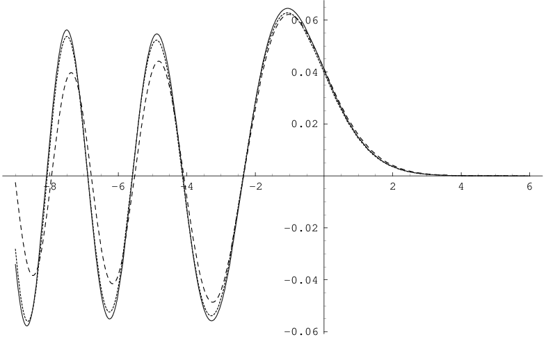
This is the desired formula for this section. Figure A.4.1 gives an illustration of our asymptotics.

Acknowledgements: This work was done as part of the author’s doctoral thesis requirements under the supervision of Professor Craig A. Tracy. The author would like to thank Professor Tracy for the discussions that initiated this work and for the invaluable guidance and support that helped complete it. Furthermore, the author wishes to acknowledge helpful discussions with Professor Harold Widom. This work was supported in parts by the National Science Foundation under grant DMS–0304414 and by the VIGRE grant-0135345.

References

[1] G. Anderson and O. Zeitouni. Lecture Notes On Random Matrices. Preprint.
[2] P. Deift. Orthogonal Polynomials and Random Matrices: A Riemann-Hilbert Approach. American Mathematical Society. Courant Lecture Notes 3, 2000.
[3] P. Deift, Universality for mathematical and physical systems preprint, arXiv:math-ph/0603038.
[4] M. Dieng and C. A. Tracy. Application of random matrix theory to multivariate statistics. preprint, Arxiv:math.PR/0603543.
[5] N. El Karoui. On the largest eigenvalue of Wishart matrices with identity covariance when $n$ , $p$ and $p/n$ tend to infinity. ArXiv:math.ST/0309355.
[6] W. Feller. An Introduction to Probability Theory and Its Applications ,Vol.II. Second edition, John Wiley, 1971.
[7] T. M. Garoni, P. J. Forrester and N. E. Frankel. Asymptotic corrections to the eigenvalue density of the GUE and LUE. arXiv:math-ph/0504053 v1
[8] I. Gohberg, S. Goldberg, and M. A. Kaashoek. Classes of Linear Operators, Vol. I, volume 49 of Operator Theory: Advances and Applications. Birkhäuser, 1990.
[9] I. Gohberg, S. Goldberg, and M. A. Kaashoek. Classes of Linear Operators, Vol. II, volume 63 of Operator Theory: Advances and Applications. Birkhäuser, 1993.
[10] I. C. Gohberg, M. G. Kre $\breve{i}$ n. Introduction to the Theory of Linear Nonselfadjoint Operators, volume 18 of Translations of Mathematical Monographs. American Mathematical Society, 1969.
[11] H. Hochstadt. The Functions of Mathematical Physics, volume 23 of Pure and Applied Mathematics: A series of texts and Monographs . Wiley-Interscience, 1971.
[12] I. M. Johnstone, On the distribution of the largest eigenvalue in principal component analysis, Ann. Stats., 29(2):295–327, 2001.
[13] P. D. Lax. Functional Analysis Wiley-Interscience, 2002.
[14] M. L. Mehta. Random Matrices, Revised and Enlarged Second Edition. Academic Press, 1991.
[15] F. W. J. Olver. Asymptotics and Special Functions Academic Press, New York, 1974.
[16] M. Plancherel and W. Rotach. Sur les valeurs asymptotiques des polynomes d’Hermite Comm. Math. Helv. 1 (1929)227-254.
[17] A. Soshnikov. Universality at the Edge of the Spectrum in Wigner Ranom Matrices. J. Stat. Phys., 108(5–6):1033–1056, 2002.
[18] G. Szegö. Orthogonal Polynomials. American Mathematical Society Colloquium Publications Volume 23
[19] C. A. Tracy and H. Widom. Level–spacing distributions and the Airy kernel. Commun. Math. Physics, 159:151–174, 1994.
[20] C. A. Tracy and H. Widom. Fredholm determinants, differential equations and matrix models. Commun. Math. Physics, 163:33–72, 1994.
[21] C. A. Tracy and H. Widom. On orthogonal and symplectic matrix ensembles. Commun. Math. Physics, 177:727–754, 1996.
[22] C. A. Tracy and H. Widom. Correlation functions, cluster functions, and spacing distributions for random matrices. J. Stat. Phys., 92(5–6):809–835, 1998.
[23] C. A. Tracy and H. Widom. Airy kernel and Painlevé II. In Isomonodromic deformations and applications in physics, volume 31 of CRM Proceedings & Lecture Notes, pages 85–98. Amer. Math. Soc., Providence, RI, 2002.
[24] C. A. Tracy and H. Widom. Distribution functions for largest eigenvalues and their applications. In Proceedings of the International Congress of Mathematicians, Beijing 2002, Vol. I, ed. LI Tatsien, Higher Education Press, Beijing, pgs. 587–596, 2002.
[25] C. A. Tracy and H. Widom. Matrix kernels for the Gaussian orthogonal and symplectic ensembles. Ann. Inst. Fourier, Grenoble, 55, 2197–2207, 2005.
[26] E. T. Whittaker and G. N. Watson. A Course of Modern Analysis Fourth Edition Cambridge University Press, 2004.