A Comparison of Information Concerning the Regression Parameter in The Accelerated Failure Time Model under Current Duration and Length Biased Sampling: Does it Pay to be Patient?
Bert van Es , Chris A.J. Klaassen , Philip J. Mokveld
Abstract: Longitudinal observations are sometimes costly or not available. Cross sectional sampling can be an alternative. Observations are drawn then at a specific point in time from a population of durations whose distributions satisfy a core model. Subsequently, one has a choice. One may process the data immediately, obtaining so called current duration data. Or one waits until the sampled durations are known completely obtaining the full durations via length biased sampling. We compare the Fisher information for the Euclidean parameter corresponding to an Accelerated Failure Time core model when the observations are obtained by either current duration or length biased sampling.
MSC 2000: 62N02, 62D05
Key words: Survival analysis, semiparametric statistics, cross
sectional sampling
1 Current duration and length biased sampling from the AFT model
Two often used models in survival analysis based on longitudinal data are the Cox Proportional Hazards model (PH) and the Accelerated Failure Time (AFT) model. These two semiparametric models both have appealing interpretations and their properties are well understood. For instance information bounds and efficient estimators of the Euclidean regression parameter are available for both models.
In situations where longitudinal observations are costly, or not available, one has to resort to technically more complicated but less costly sampling schemes, like cross sectional sampling. In a medical setting this means that instead of following a certain number of patients in time one selects the durations of the disease of a group of patients sampled at a specific point in time, obtaining a so called cross sectional sample. One then has a choice. Either one uses the data at hand at the time of sampling, i.e. the durations up to the present, obtaining so called current duration data, or one decides to wait until the full durations for the sampled patients are known. Because longer durations turn out to be sampled more frequently than shorter ones, the second type of sampling is known as length biased sampling.
Let us compare the two cross sectional sampling regimes. Current duration sampling will only require knowledge of the duration up to the present and is thus very cheap in this sense. Length biased sampling requires the time needed to observe the full durations of the diseases of the patients that have been sampled and is thus more costly than current duration sampling.
We will assume that we sample from a population of durations that satisfy a semiparametric core model. By comparing information bounds for the Euclidean parameter under the two cross sectional sampling schemes we will investigate the gain in efficiency in being patient.
Our comparison below is based on results for current duration and length biased sampling for the AFT core model in these situations, presented in Mokveld (2006). Similar results for the PH model do not exist at present. See also Van Es, Klaassen and Oudshoorn (2000) for some general features of current duration sampling.
1.1 The core AFT model
We first introduce the AFT core model. Let denote a duration, for instance the duration of the disease of an individual from a homogeneous group of patients with a particular disease, and let denote a vector of covariates of dimension with density with respect to a measure . We do not assume knowledge of . Let denote an unknown -vector of regression parameters.
The semiparametric AFT model for the random vector is given by
| (1) |
where is a nondegenerate random variable on with unknown absolutely continuous distribution function , with density and hazard function , and where and are independent. We consider estimation of , treating as a nuisance parameter .
From the model equation (1) we can derive the conditional survival function , the conditional density and the conditional hazard function of given . We get, for ,
Note that given the value of the covariate vector the model is a scale model. The function serves as baseline hazard in this scale model. Depending on the value of the scale on average the duration is decreased or increased.
Also note that taking logarithms in the model equation (1) we get
showing that the AFT model is actually a regression model for the logarithm of the duration. However, differences are caused by different natural assumptions on the distributions of in the AFT model and the error in the regression model.
1.2 Current duration and length biased sampling
Let us assume that we observe the durations and their covariates at a specific point in time, the present. Let denote the total length of a sampled duration and let denote the time from onset until the present of a sampled duration.
For simplicity we first describe the sampling distributions in the situation without covariates. If and are the density and distribution function of the durations in the core model then under suitable assumptions the densities of and equal
| (2) | ||||
| (3) |
where and . It turns out that is in distribution equal to with uniformly distributed on the unit interval and with and independent. Hence, while formula (2) follows from the length bias in the sampling, formula (3) follows from the same length bias in selecting the duration and from multiplicative censoring, since at the present we only observe a fraction of the total duration!
The formulas (2) and (3) require suitable models for the times of onset of the disease. In Van Es, Klaassen and Oudshoorn (2000) and Mokveld (2006) two models for the times of onset are described that give rise to the densities above.
One can follow a direct approach where the random variable denotes the time of onset and is uniformly distributed on the interval . Subsequently one lets go to infinity. The duration is assumed to be independent from and current duration sampling takes place at time zero. A duration is sampled if and only if (random left truncation). The disease will have lasted at time zero and will last if we wait until recovery. The distributions of and can be computed by conditioning on .
Following Keiding (1991) one can also follow a point process approach where patients get ill at the time points of a stationary Poisson process with constant intensity . The durations of their disease are modelled as i.i.d random variables that are independent from the Poisson process and cross sectional sampling takes place at some fixed point in time. By point process techniques one can show that , the number of durations that are sampled, has a Poisson distribution, and, conditionally on , the sampled times from onset and full durations are i.i.d. with the densities (2) and (3).
In the regression setting with covariates we observe i.i.d. realizations of or of durations (in total or from onset to present) and the sampled covariates. As mentioned above we consider the case where the density of the covariate in the core model is unknown. Under the AFT model assumptions for the core model, it turns out that given the covariate the distributions of both and belong to scale parameter families, just as the distribution of the original durations in the core model. In fact, they again follow an AFT model. The difference with the core model is that now the distribution of , the observed covariate, depends on the Euclidean parameter . It does not depend on !
For , and we have for the total duration
| (4) | ||||
and for the duration from onset to present
| (5) | ||||
These formulas hold under the direct approach or the point process approach for the times of onset described above. See Van Es, Klaassen and Oudshoorn (2000) or Mokveld (2006) for details.
2 A comparison of information bounds
We will present information bounds for estimation of the Euclidean parameter for cross sectional sampling from a core AFT model as derived in Mokveld (2006). Throughout, when we mention information we mean information contained in one observation.
As above, primarily we consider the case where the covariate distribution is unknown. See Remark 2.1 for the case where this distribution is known.
2.1 Current duration and length biased sampling
The covariance matrix of the sampled covariates appears in all information matrices below. It equals
Note that this matrix depends on through the distribution of .
Let us first define the Fisher information for scale for a density
| (6) |
With , equal to and equal to , it is shown in Mokveld (2006) that efficient estimators of can be constructed and that the information bounds are equal to
in the situation of length biased sampling where the full durations are observed, and to
in the situation of current duration sampling where the durations from onset to present are observed. Rewriting and in terms of we get
and
Remark 2.1.
Let us consider the model where the covariate distribution in the core model is known. Then (4) and (5) show that the distribution of the covariates in the sample is the same for current duration and length biased sampling, that it does not depend on , and that the Fisher information matrix in one observation for based on the covariates in the sample alone is equal to . Under suitable assumptions can be estimated -consistently from the covariates alone by for instance the maximum likelihood estimator.
The information for based on durations and covariates now equals
in the situation of length biased sampling where the full durations are observed, and to
in the situation of current duration sampling where the durations from onset to present are observed. These are obviously larger than in the situation where the covariate distribution is unknown.
Note also that, using both durations and covariates in the sample, the semiparametric information for , with as nuisance parameter, under the two sampling schemes, is larger than , the information based on the covariates alone.
2.2 A comparison
The results in this section show that it pays to be patient.
Theorem 2.2.
Let be an absolutely continuous density on with derivative a.e. and let . Let be equal to and let be equal to . If and are finite then
| (7) |
holds.
Proof.
Note that is the density of and that is the density of . Since , with independent of and uniformly distributed on the unit interval, we have
So the relation between and can be expressed as
| (8) |
By expanding the square in (6) we see that the inequality (7) holds if and only if
| (9) |
Let vanish at and be differentiable at with derivative . Since is nonnegative Lebesgue a.e., we get . Because an absolutely continuous function is Lebesgue a.e. differentiable, this shows that is a Lebesgue null set. Consequently by the Cauchy-Schwarz inequality we have
Hence by (8) we have
which completes the proof of the inequality provided that we show that equality can not occur.
The fact that the inequality (7) is strict can be seen as follows. The Cauchy-Schwarz inequality holds with equality if and only if
for some constant and for all . But for equality to hold in (9) this last equality has to hold for all . Now writing this condition equals
for all and all , which can obviously never hold. ∎
Actually, this theorem is a consequence of a more general inequality for Fisher information for scale for a product of random variables.
Theorem 2.3.
Let be a density on that is absolutely continuous with respect to Lebesgue measure with derivative , such that , as defined by (6), is finite. If is an arbitrary distribution function on and the density is defined by
then
with equality iff is degenerate.
Proof.
Let be a random variable with density The random variable has density then with One may verify that the Fisher information for scale of equals the Fisher information for location of Furthermore, is the density of the product of and a random variable with distribution Consequently, with defined by and defined by , it suffices to prove that holds with equality iff is degenerate. However, this inequality follows by Cauchy-Schwarz via
as has been noticed by Hájek and Šidák (1967) in their Theorem I.2.3 on page 17. ∎
2.2.1 Examples
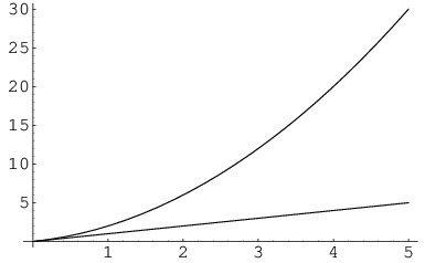
To get a feeling for the difference in information in the current duration and length biased observations we consider two families of densities for the nuisance parameter , the Weibull densities and the log logistic densities.
First we consider the Weibull densities. Let be a Weibull density with parameter , i.e.
For these densities we have

Next we consider log logistic densities . Let be a log logistic density with parameter , i.e.
For these densities we have

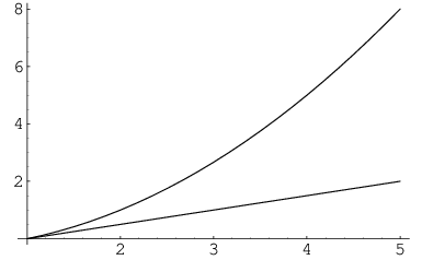
These two examples show that the more concentrated the density of the random variable in the model (1), corresponding with high parameter values , the higher the gain in being patient.
References
- [1] B. van Es, C. A. J. Klaassen, and K. Oudshoorn. Survival analysis under cross sectional sampling. Prague Workshop on Perspectives in Modern Statistical Inference: Parametrics, Semi-parametrics, Non-parametrics (1998). J. Statist. Plann. Inf., 91:295–312, 2000.
- [2] J. Hájek and Z. Šidák (1967). Theory of Rank Tests. Academic Press, New York-London; Academia Publishing House of the Czechoslovak Academy of Sciences, Prague, 1967.
- [3] N. Keiding. Age specific incidence and prevalence: a statistical perspective. J. Roy. Statist. Soc. Ser. A, 154:371–412, 1991.
- [4] Ph. J. Mokveld. The Accelerated Failure Time Model under Cross Sectional Sampling Schemes. Ph.D. Thesis, University of Amsterdam, in preparation.
Bert van Es: University of Amsterdam, Korteweg-de Vries Institute for Mathematics , Plantage Muidergracht 24, Amsterdam, 1018 TV, The Netherlands, vanes @science.uva.nl
Chris A.J. Klaassen: University of Amsterdam, Korteweg-de Vries Institute for Mathematics , Plantage Muidergracht 24, Amsterdam, 1018 TV, The Netherlands, chrisk@science.uva.nl
Philip J. Mokveld: University of Amsterdam, Korteweg-de Vries Institute for Mathematics , Plantage Muidergracht 24, Amsterdam, 1018 TV, The Netherlands,