Nonparametric Bayesian Classification
NONPARAMETRIC BAYESIAN CLASSIFICATION
a dissertation
submitted to the department of statistics
and the committee on graduate studies
of stanford university
in partial fulfillment of the requirements
for the degree of
doctor of philosophy
Marc A. Coram
August, 2002
© Copyright by Marc A. Coram 2002
All Rights Reserved
I certify that I have read this dissertation and that, in my opinion, it is fully adequate in scope and quality as a dissertation for the degree of Doctor of Philosophy.
Persi Diaconis (Principal Adviser)
I certify that I have read this dissertation and that, in my opinion, it is fully adequate in scope and quality as a dissertation for the degree of Doctor of Philosophy.
Jerome H. Friedman
I certify that I have read this dissertation and that, in my opinion, it is fully adequate in scope and quality as a dissertation for the degree of Doctor of Philosophy.
Bradley Efron
Approved for the University Committee on Graduate Studies:
Abstract
A Bayesian approach to the classification problem is proposed in which random partitions play a central role. It is argued that the partitioning approach has the capacity to take advantage of a variety of large-scale spatial structures, if they are present in the unknown regression function . An idealized one-dimensional problem is considered in detail. The proposed nonparametric prior uses random split points to partition the unit interval into a random number of pieces. This prior is found to provide a consistent estimate of the regression function in the topology, for any , and for arbitrary measurable . A Markov chain Monte Carlo (MCMC) implementation is outlined and analyzed. Simulation experiments are conducted to show that the proposed estimate compares favorably with a variety of conventional estimators. A striking resemblance between the posterior mean estimate and the bagged CART estimate is noted and discussed. For higher dimensions, a generalized prior is introduced which employs a random Voronoi partition of the covariate-space. The resulting estimate displays promise on a two-dimensional problem, and extends with a minimum of additional computational effort to arbitrary metric spaces.
Acknowledgements
I thank my parents, who laid the foundations of my character and have been an unfaltering source of love and encouragement. I also thank my advisor, Persi Diaconis, whose friendship, support, and insight have been vital to successfully enduring the Ph.D. process. I also wish to thank the other members of my examining committee: Jerome Friedman, Bradley Efron, Susan Holmes, David Siegmund, and Hans Andersen, for their professionalism and patience. Finally, I thank Hua Tang for putting up with my quirks all these years.
Chapter 1 Introduction
The binary classification problem is perhaps the simplest regression problem, but it continues to pose fresh challenges. In the binary classification problem, we are given a list of pairs each pair drawn independently from an unknown probability measure . The ’s play the role of covariate or “predictor” and lie in some abstract space , while the ’s are interpreted as a class label and are either 0 or 1. Our goal is to estimate certain functionals of . Specifically, in the binary regression problem, we are interested in estimating the regression function . The value of at a given point is the conditional probability that given that . In this way we model the joint distribution by saying that to draw an pair from , first draw a covariate from the marginal distribution of denoted by . Then “flip” an coin to determine the value of .
In the classification problem, we are concerned with being able to predict future values. The standard formalization of this task is that we wish to choose the “decision rule” that will minimize the expected loss incurred; this reduces to the problem of estimating the set , for some that depends upon the loss (for simplicity, ignore the possibility that depends on ). There are a great many ways to proceed on each of these problems, as demonstrated by the vast literature on these subjects. Some references are given in section 2.3.
In this thesis, I propose a nonparametric Bayesian approach to the binary classification and regression problems. Specifically, to derive an estimator, I regard itself as random. For simplicity, I regard the marginal distribution of , as known. In this case, putting a prior distribution on amounts to putting a prior on . More generally, one can also put a prior on functions and suppose that . Some sort of mild restriction, like this one that all share some dominating measure , is useful to avoid technical problems in defining the conditional distribution of given the data.
Let denote a prior distribution on , or, more precisely, on pairs. Extend to a joint distribution on and the infinite data sequence which, conditionally on , is drawn independently and identically distributed () from . Formally, the posterior is the measure . In practice Markov chain Monte Carlo procedures can be used to generate a sample from the posterior.
The posterior mean of is an important summary of the posterior: its value minimizes the posterior risk under an loss. Let denote the posterior mean: . Another important summary of the posterior is the classification rule which minimizes posterior misclassification loss. If asked to predict the most likely value of the ’s corresponding to , …, all at once, the decision that would minimize the posterior-expected --loss is simply . Interestingly, though, if asked sequentially instead of all at once, it is necessary to update with each new data point before deciding.
Taking this Bayesian approach assures us that the resulting estimators will have a clear subjective interpretation. In addition, if the prior is carefully chosen, the resulting estimators, chosen indirectly through this Bayesian framework, may have frequentist advantages over the estimators that might otherwise be proposed. For example, interesting kinds of shrinkage and averaging occur automatically within this framework. Subsequent chapters assess the frequentist performance of these Bayesian estimates by simulation experiments (chapter 4) and theoretically (chapter 5).
1.1 An Example
To get started, let us consider the specific case in which and the sampling distribution of the , , is known to be the distribution. Further, let us consider a specific which is complicated enough that its estimation should not be too easy for any of the standard methods; it is piecewise continuous with two constant regions and a smooth transition region. As shown in Figure 1.1.b, is chosen as:
where is the density of a normal with mean 0 and standard deviation .
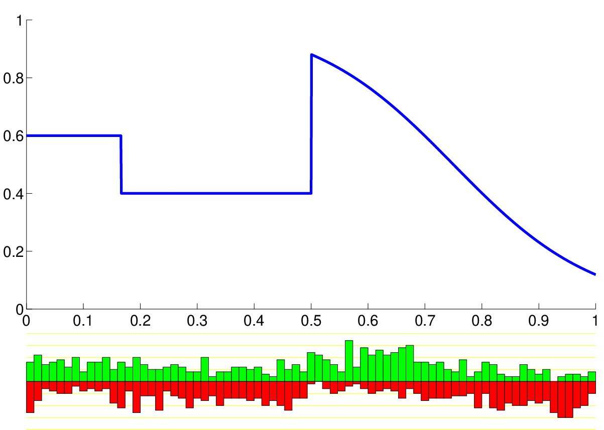
The two histograms in Figure 1.1.b summarize a simulated data set of 1024 data points that was drawn from this model. The green histogram is a histogram of the heads. The red histogram is a histogram of the tails; it is drawn upside down to facilitate comparison with the green histogram. To more easily interpret this display, notice that if we take the sum of the corresponding green and red bins at each point, we recover a histogram of the marginal distribution, which is uniform. Furthermore, the ratio of the height of a green bin to the corresponding red bin represents the empirical odds of a head in that bin. Near , for example, notice the sharp transition from nearly equal green and red bins (on the left) to much longer green than red bins (on the right). The performance of this posterior mean estimator is compared with a variety of more conventional methods in chapter 4. This example is used to illustrate the present approach in the rest of this introduction.
1.2 A Nonparametric Prior on Regression Functions
To specify a prior over functions , I explain how to choose , at random from it. This completely specifies a prior on the probability distribution , since I consider the marginal distribution to be known. The prior on will concentrate on locally-constant step functions. To choose a step function at random, first, choose , the number of locally constant intervals, where:
That is, is with parameter . Ultimately, the choice of must be specified by the user. For the examples in this thesis, I have used unless otherwise noted. This choice seems to perform well. For further discussion of how to choose a prior on which results in provably consistent estimators, see chapter 6.
Now, conditional on , choose iid from . Let (for ) be the ordered value of the ’s. This produces intervals:
If , simply take . Finally, conditional on , choose values (for ) iid from . This generates the random function :
1.3 Sample Results

Conditioning this prior on the data described in the earlier example section results in a posterior distribution on regression functions . Applying the techniques in chapter 3 to sample from the posterior results in a long list of sampled functions. Although the prior specified a prior distribution on the number of locally-constant pieces in each function, when drawn from the posterior, functions typically have at least 5 pieces. Taking the average of these functions (at every ) gives an estimate of the posterior mean; this is illustrated in Figure 1.3.b. Further discussion of results like this can be found in chapter 4.
1.4 The Partitioning Approach
Step functions, such as the functions that the prior concentrates on, have the advantage of great mathematical simplicity; but, if specified in sufficient detail, they can approximate general functions. For a multi-dimensional regression function, it is natural to generalize this idea by considering some partition of the covariate space into a number of pieces and constructing a function that takes a different value on each piece. A procedure that uses a wide variety of geometric shapes to partition the space might be able to find a partition with the right structure to approximate the unknown regression function. Ideally, the partition would be no more complex than necessary to achieve a good approximation. If the unknown regression function has certain global features that the chosen partition can be adapted to, this idea becomes very powerful. Instead of merely “borrowing strength” locally, like ordinary smoothing estimators do, a partition-based estimator borrows strength across the whole range of a partition element. As a simple example, if the true regression function does not depend on one of the covariates, the partition elements do not need to break up space along this dimension at all; this results in larger partition elements and more efficient estimation of the success probability on each of the pieces. Similarly, if the regression function is almost flat in some large chunk of space, then this whole region can become a single element. If the level-sets of the regression function have smooth boundaries, perhaps the partition elements can be chosen to follow these contours. Finally, since the best partition for the unknown function is unknown, it makes sense to average together the approximations found by a variety of partitions that make the data likely. This is exactly what the posterior mean estimate will do automatically. Chapter 7 shows one way in which this idea can be applied using Voronoi partitions. For this partition, a prior distributes seed-points in the covariate space; each seed corresponds to a partition element, the one that consists of all points closer to that seed than any other seed. By placing the seeds appropriately, the partition can be fine or coarse as needed. The boundary between partition elements is itself a hyperplane whose position and orientation can be controlled through the placement of the seeds.
Other authors have recently considered similar priors with good success. Their work is discussed in section 2.2. To the best of my knowledge, this thesis presents the first theoretical examination of consistency issues for priors of this sort (c.f. chapter 5, with discussion in chapter 6). Additionally, I present a detailed assessment of the empirical performance of my methods on certain novel simulation experiments. The comparison with bagged CART regression trees in chapter 4 is especially interesting.
1.5 Outline
Chapter 2 gives a literature review. Chapter 3 shows how to (approximately) compute samples from the posterior and the posterior mean. Chapter 4 trys out the method on examples and carefully compares its performance with that of a variety of existing methods. Chapter 5 gives sufficient conditions on the prior under which it provides universally consistent estimates of . Chapter 7 describes a different prior which extends these ideas to general metric spaces by employing random Voronoi partitions. Certain modifications are explained that make the proposal more practical and its performance on an example is shown. Finally, the afterword gives a philosophical argument that advocates the use of Kolmogorov-complexity in future statistical thinking.
Chapter 2 Literature
This chapter reviews and discusses the literature on three subjects. The first section reviews some theoretical results concerning the frequentist performance of Bayesian procedures. The second section gives a survey of some of the work done by authors on related Bayesian efforts. The final section briefly surveys some salient examples of alternative approaches to the classification problem.
2.1 Theoretical Results
The frequentist performance of Bayesian methods is of fundamental interest in statistics. Given a large sample from a smooth, finite-dimensional statistical model, the situation is quite well understood. The Bernstein-von Mises theorem [49, 33] shows that the Bayes estimate and the maximum likelihood estimate will be close. Furthermore, the posterior distribution of the parameter vector around the posterior mean is close to the distribution of the maximum likelihood estimate around the truth: both are asymptotically normal with mean 0 and the same covariance matrix. Unfortunately, though, in more general circumstances, such as those needed for this work, the situation can be much more complex. In particular, the basic model is based on an infinite hierarchy of finite dimensional models. Moreover, even for a given finite dimensional submodel, the dependency of the likelihood function on the parameter is not smooth; the functions are allowed to take jumps. Consequently, a more general theory is needed.
This section reviews some of the literature on this subject with a focus on results that address the question of consistency: i.e. as the number of data points tends to infinity, will the Bayesian estimate converge to the true value (in some suitable sense) almost surely (resp. in probability)? The literature contains a number of useful and quite flexible positive results, but also a variety of interesting negative examples showing that the regularity conditions under which the theorems hold are not to be taken lightly. A good introduction to these issues is by Diaconis and Freedman [23]. Throughout this section, the reader may envision a family , a prior , and posterior , where the are drawn iid from . Consistency means that the posterior concentrates at for large samples.
Doob [29] established a fundamental result under minimal regularity assumptions using a martingale convergence argument. Roughly speaking, the result states that if consistent estimators exist at all, then a Bayes procedure will provide an almost surely consistent estimate of the true parameter under sampling from the distribution for any in some set which has prior probability of . Notice, though, that this does not specify if consistency will obtain at any particular point of interest , unless happens to be a point-mass of the prior, or unless it possible to determine by some more detailed line of argumentation.
Freedman [32] considered the case in which the observations are discrete. If the set of possible observations is finite, the posterior is consistent exactly for parameter values in the topological support of the prior. The countably infinite case is more complex. He constructs a class of examples showing that it is possible to construct a prior which assigns positive mass to every (weak star) neighborhood of the true parameter value, but for which the posterior converges to a point mass at some other (chosen) parameter value. Furthermore, he finds a prior which assigns positive prior mass to every (weak star) open set of parameters, but for which the posterior is consistent only at a set of parameters of the first category. The reader should note that this prior did not assign mass to all entropy-neighborhoods. This sort of subtle distinction can make all of the difference and explains the necessity of some such assumption in the following consistency theorems. He introduces the “tail-free” priors for the the countably-infinite case and demonstrates that these are always consistent.
Lorraine Schwartz [61] explored the question of consistency in a very general setting. She extended Doob’s result to a broad class of loss functions [61, lemma 4.2]. She also found sufficient conditions for the posterior to be consistent under sampling. These conditions, she says, are “of an essentially weaker nature” than the conditions established for the consistency of maximum likelihood estimators. Nevertheless, she constructs an example where the maximum likelihood estimate is consistent and the estimates based on certain priors are not. The example ([61, example 3]) involves a simple parametric family of densities which satisfies Wald’s conditions, thereby guaranteeing that the maximum likelihood estimate will be consistent, but for which the posterior can be inconsistent. The consistency of the posterior in this case, is found to depend critically on the amount of mass that the prior ascribes to small neighborhoods of the true parameter value; if this mass shrinks too quickly, the prior “ignores” the data. One clever aspect of her construction is the way the densities are parametrized. Parameter values close to the target value correspond to densities that are close to the -density in an sense, but which are farther and farther away in Kullback-Leibler discrepancy. In fact, there is only one point in parameter space (the true parameter) that has Kullback-Leibler discrepancy from the truth smaller than , for sufficiently small.
Schwartz then shows that the posterior will be consistent under sampling under two basic conditions. First, the prior should have positive mass on Kullback-Leibler neighborhoods of the true parameter (defined in section 5.1 of this thesis), and second, the model class should not be too rich; specifically, she requires that uniformly consistent tests of the hypothesis that against the alternative that lies outside a given (open) neighborhood of exist.
It is not always obvious how to verify the later property directly. Modern authors have employed entropy-type bounds to guarantee their existence. Ghoshal, Ghosh, and van der Vaart [40] state a theorem ([40, theorem 7.3]) which proves that the posterior converges at a certain rate if certain uniform tests exist (and the prior mass is suitably distributed) and go on to find a variety of entropy-type conditions that suffice to be able to construct the necessary tests. Shen and Wasserman [62] show related results, requiring slightly different conditions on how mass needs to be allocated–they do not a make a connection with testing. Barron, Schervish, and Wasserman [2] find sufficient conditions for the posterior to be consistent; their results are reviewed and then used in chapter 5.
It should be noted that these various conditions for consistency are not necessary, but merely sufficient. Nevertheless, it is important to treat this subject with care because of the variety of examples for which consistency fails.
Barron, Schervish, and Wasserman also give an interesting example where consistency fails. In this example, they show that the prior puts too much mass on a very rich class of models that will be able to match any spurious structure that the data might have by chance, overwhelming the true parameter. Furthermore, lest the reader get the wrong idea, inconsistency does not only occur in artificial examples. A series of “natural” yet still inconsistent estimators for the symmetric location problem are discussed by Diaconis and Freedman [23]. In addition, the binary regression example explained in the next section has a natural motivation based on conditional exchangability.
2.2 Related Bayesian Work
The following subsections contain a review of work by other authors that is closely related to this thesis. It is followed my a brief synopsis of the contributions that this thesis makes to the literature.
2.2.1 A Dyadic Prior for Binary Regression
The most relevant examples for the work of this thesis are the nonparametric binary regression examples of Diaconis and Freedman [24, 25]. They use a different prior; call it , a hierarchical, dyadic prior on . To describe , let be the set of intervals which result from partitioning the unit interval into equal pieces. Let be the subset of functions which are constant on all intervals . Finally, fix a prior distribution on the non-negative integers. Assume, for simplicity, that for all . To draw from , draw from and then, conditional on hierarchy-level , draw uniformly at random from . In effect then, at level one draws independent random variables to describe the success probability on each of the pieces.
They show that for any and any (except possibly for ), the posterior estimates are consistent (in the sense that any neighborhood of has posterior probability tending to a.s.). Remarkably, however, for , the posterior can be an inconsistent estimate if the tail of is sufficiently heavy. Specifically, let . Then if , the posterior is inconsistent at . On the other hand, if , the posterior is consistent for any . To put this in perspective, for (a shifted prior), . The critical value for is ; for larger (longer tails) inconsistency will occur (but only for ).
This result is substantially stronger than the result I have obtained for my prior . In particular, applying the same (general) method of proof that I employed to prove consistency for to yields only the result that is consistent if the tails of drop off at least as fast as those of a Poisson. (Recall, that at level , only divides into intervals, but divides it into .) Their method of proof is direct: using Bernstein’s inequality, Poissonization, and special features of the prior. My method of proof is indirect; it uses general results that employ entropy-type bounds.
There are striking similarities between and . In fact, is equivalent to a suitably randomized . To achieve this, it is not enough to simply randomize the dyadic split points. Instead, recall that has an alternative interpretation in terms of binary sequences. At hierarchy-level , is uniform over . This corresponds to independently assigning uniform success probabilities to each binary sequence of length . Here is an alternative way to draw from . Draw from and interpret as function on binary sequences of length ( depends on ). Let () be random variables. To any point associate the binary random variables (). Define via . Note that only a small fraction of possible binary sequences are realized in this manner (at level (which ranges from to under ), sequences out of the full set of possible sequences are achieved).
2.2.2 Bayesian CART
Two other closely related priors can be described as Bayesian versions of the CART algorithm. This was pursued by Chipman, George, and McCulloch, whose prior closely parallels the choices made in the original CART algorithm [6, 7, 8, 9]. Here is a description of their prior when the covariate space is . Their prior starts with a root node (which represents the whole space); this node is then recursively partitioned in a random way. For each node, randomly choose whether to split it or not, then choose a coordinate to split on, then choosing a split point (i.e. the cutoff value) randomly from among the midpoints between the ordered values of this coordinate; finally each leaf node is given an independent regression value. The details of how these decisions are made differ in their particulars from the ones that I described in the introduction. In early work, these authors observed that using MCMC to sample from the posterior of this prior provides a rudimentary (global) search procedure, which has certain (apparent) advantages over the greedy search procedure commonly implemented in CART-type algorithms. In later work, they examined and computed the (approximate) posterior mean (working primarily on the least-squares white-noise regression problem) and found that it had good performance. They also considered extended priors that modeled the regression values as additively (not independently) generated [9].
Denison, Mallick, and Smith, independently considered another version of Bayesian CART [18, 17, 19]. For one-dimensional problems they propose using random splines (the prior I use is essentially a special case of this prior). They consider some of the regression examples that are standard in the wavelet literature and show that their spline methods perform equally well. Additionally, they propose a Bayesian version of Friedman’s MARS which puts a prior on functions that are constructed by adding together random spline-type ridge functions. Denison, Adams, Holmes, and Hand discuss the usefulness of random partitions in this paper [15].
Very recently, Denison, Holmes, Mallick, and Smith have written a book [16] which surveys some related Bayesian regression schemes, including a Bayesian method for (multiple class) classification using Voronoi partitions that is very closely related (albeit independent of) the work that I present in chapter 7. The book also discusses Bayesian wavelet methods, and an interesting Bayesian nearest-neighbor prior. As a default prior, they recommend assuming that every model in a “single dimension” is equally likely, and each dimension is equally probable, a priori. This “flat prior,” they claim, should serve perfectly well because of the, “natural tendency” for the marginalized likelihood to penalize complex models:
On the face of it, we might be concerned that the flexible modeling strategy we advocate might be prone to overfitting the data by adding too many basis functions. Indeed, many papers found in the literature advocate explicit priors on the model space that penalize the dimension of the model. However, throughout this book we argue that such a measure is unnecessary. The Bayesian framework contains a natural penalty against over [sic] complex models, sometimes called Occam’s razor, which essentially states that a simpler theory is to be favoured over a more complex one, all other things being equal.
There is no consideration given to the possibility that this might give rise to inconsistent estimates (e.g. as in the Diaconis and Freedman non-parametric regression example explained earlier); indeed there are few theoretical considerations at all in the book. Their explanation of why the Markov chain techniques that they develop should actually give meaningful samples from the posterior appeals to Green’s reversible jump [41]. The explanation given is vague and ultimately they decide to avoid the issue and appeal to the fact that their chains are discrete. The chains in chapter 3 of this thesis involve a continuous state space and do not simply avoid this issue by discretizing the continuous modeling space as these authors seem to do.
Overall, the book emphasizes main ideas, algorithms, and results. It seems that for every existing regression technique, they want to demonstrate that they can make a “Bayesian” version of it too. The book does not emphasize subjectivism, but rather adopts an “” perspective to Bayesian modeling: “we never believe that the true model lies in the set of possible models.” The book does do a good job of supplying default priors for a wide variety of possible parametric models. Similarly, Denison’s thesis [20] emphasizes the wide variety of problems to which Bayesian partitioning methods of this sort can be applied.
2.2.3 Poisson Rate estimates using Random Partitions
Green [41], and Scargle [58] develop priors on piecewise constant functions on the real line and using Voronoi cells. Their priors are quite similar to the ones developed in this thesis, but are intended to address the problem of estimating the rate function of a process. In principle, one could apply their techniques to the problem of binary regression by generating an estimate of the rate function of the “heads” process and the “tails” process separately and then combining the results. I do not think that this has been tried and it seems substantially less “natural.”
Green applies his method to a coal mining dataset and a synthetic two-dimensional example. For these example, Green assumes that an individual cell’s rate-parameter is drawn independently from a prior. For the one-dimensional case he advocates a prior which “probabilistically” spaces out the change-point locations; specifically, if there are change-points, the ordered locations of the change-points are distributed like the even order statistics of independent uniform values. He argues that this is good because it prevents small change-point intervals from entering into the posterior. For the two-dimensional example, the generating points of the Voronoi partition are drawn independently and uniformly. Green’s methods are given, in part, as examples of his “reversible jump” MCMC technique. This technique has become an accepted part of MCMC practice, but is not accepted by all experts in MCMC theory because it does not lay down in a straightforward “theorem-proof” manner the necessary conditions and consequent conclusions. For this reason, detailed verifications for the chains used in this thesis are given in chapter 3.
Scargle’s work is applied to astronomical data; he concentrates on the problem of finding the mode of the posterior, rather than the posterior mean. Fortunately, he and coworkers have developed a way of computing this mode in the one-dimensional case exactly and efficiently using a dynamic programming approach [59]. Instead of giving each cell an independent value, Scargle gives each cell a (logical) “color” and then associates each unique color with an independent rate-parameter. This allows him to use a fine partition and then group “chunks” back together into more complicated shapes. The way he forms this partition is also different; in particular his “prior” is data dependent, but not quite in the way of the “prior” that I consider in chapter 7. Rather, the data is used once and for all to generate the fine Voronoi partition of space that results from using all of the data points as generators. These cells are then “clumped” (i.e. given a logical color) and the clumps are given an independent rate parameter.
2.2.4 Bayesian “Image” Analysis
Møller and Skare [53] apply their work to reservoir modeling and connect their work to efforts in Bayesian image analysis (including Markov random fields). They use a random Voronoi partition of the data and assign each partition element a random color (in a way that depends only the colors of neighboring cells). They supply several further references to work in Bayesian image analysis which use Voronoi cells. From their perspective, to calculate their posterior they are simulating from a special “marked point” process. The generators of the Voronoi cells are regarded as point set that has been drawn from a homogeneous Poisson process of rate on the unit cube. In the simplest case, the marks or “colors” of these points are just integers from up to that have been drawn independently. More generally, according to their prior, the conditional distribution of the coloring of cells given is an Ising or Potts model. The graphical structure of this model is determined by consideration of which Voronoi cells are neighbors, and the parameter is chosen to reflect their prior belief that neighboring cells tend to be of the same color. They consider two problems. The first is a simulation experiment in which a “true” binary image is degraded with Gaussian noise. The second is a three dimensional reservoir problem based on real data. It is supposed that a certain three dimensional cube (the reservoir) consists of 4 different types of rock. The rock types are observed along seven vertical lines, representing the observations of rock that were made as seven wells were dug into the reservoir. In both problems, the true object to be recovered is itself a certain “coloring” of space (i.e. rather than a continuous regression function). For the MCMC computation of their posterior they apply the birth-death type Metropolis-Hastings algorithm for point processes, as studied by Geyer and Møller [38] and claim that their target distribution satisfies a local stability condition (see Geyer [37], Kendal and Møller [45], and Møller [52]) so that the MCMC is actually geometrically ergodic.
2.2.5 Polya Trees
Finally, Polya trees [48] and especially randomized Polya trees [55] deserve to be mentioned. The basic Polya tree puts a prior on distribution functions on the unit interval. The unit interval is divided recursively in a dyadic binary way and mass is allocated to each piece of the partition in a stagewise manner by first determining how much of the mass that is available will be on the left versus the right half and then continuing with such determinations layer by layer. Each of these assignments is ultimately determined by independent random variable, whose parameters depend upon its location in the “tree.” If a suitable choice of these parameters is made the result prior on distribution functions concentrates on distributions that are absolutely continuous with respect to Lebesgue measure. The essential advantage of Polya trees is that the posterior of Polya tree prior is easily and analytically computable, being itself another Polya tree. For randomized Polya trees, the partitioning scheme is independently “jittered” at random in a particular way [55]. A Hybrid MCMC can be employed to sample from the randomized Polya tree posterior which uses a Gibbs step to take advantage of the ease with which the (internal) Polya tree posterior can be computed. Both methods can be extended (essentially by taking “direct products”) to put a prior on distributions on the unit cube.
2.2.6 The Contributions of this Thesis
Reviewing the depth and breath of the literature reviewed above may leave the reader in doubt about the contributions of this thesis. After all the one-dimensional prior that I consider is essentially a special case of the univariate spline model and the idea of using Voronoi partitions is certainly not new, although effective Bayesian methods using them only started springing up fairly recently.
Still there is room for careful analysis. This thesis establishes that the posterior is consistent under suitable conditions on the prior and for any measurable regression function (see chapter 5 for details): an issue which none of the “Bayesian CART” or “Voronoi Partition” authors address at all. This thesis also gives an explicit Markov chain Monte Carlo algorithm (see section 3.4). Broadly speaking it is a fairly standard birth-death Markov chain as considered by Geyer and Moller [38], but the technicalities of the analysis seem to be somewhat different. This thesis proceeds to show in detail that it satisfies detailed balance by direct self-contained argumentation; further, the chain is shown to have an ergodicity property (see section 3.10). These considerations are often glossed over in modern writing.
On the more practical side, chapter 4 scrutinizes the behavior of the posterior mean estimate under a variety of carefully designed simulation experiments. These experiments both serve to analyze the posterior mean and to give insight into the relationship between Bayesian methods and their classical counterparts. See for example the discussion of CART and bagging in subsection 4.1.3.
2.3 Other Approaches
The literature on classification and regression methods is huge; the interested reader is urged to consult good modern books on the subject like The Elements of Statistical Learning, by Hastie, Tibshirani, and Friedman [43]. The following paragraphs outline some of the methods that have had the most impact upon the author.
In the statistics literature, classical approaches to the classification and binary regression problem include logistic regression, Fisher’s discriminant analysis, and projection pursuit methods. Logistic regression specifies that the success probability regression function is such that its log-odds follows a linear model with a user specified basis (e.g. by using polynomial or spline functions of the covariate-data) and estimates the parameters by maximum likelihood. Model selection is commonly performed using classical methods to select a subset of the covariate variables. Fisher’s discriminant analysis finds a hyperplane which “optimally” separates the two classes using a within versus between variance criterion. Projection pursuit seeks an interesting linear (or sometimes nonlinear) projection of the covariate-data onto a lower dimensional subspace (e.g. ). Various criteria have been proposed to define “interesting,” some of which are suitable for the classification problem. Each of these methods has undergone a variety of generalizations and tweaks to address a wider range of problems over the years.
The first general method to solve the classification problem automatically was the -nearest neighbor approach [12]. -Nearest neighbor estimates are known to be universally consistent if slowly enough [21]. Their convergence, however, especially in high dimensional problems, can be slow in practice [36].
Local regression methods are a clever extension of this approach. To predict at a given point, instead of averaging the values given at the neighbors, they fit a low-order linear model to a locally-weighted version of the data set [10].
Trees [4] and neural nets [56] differ in that they search through a globally-parametrized class of functions. In all of these methods, cross-validation is often employed to estimate frequentist “out-of-sample” performance and select a regularization parameter which governs the trade-off between bias and variance [43].
Wavelet methods are in some ways a compromise between the local and the global approaches mentioned above. They fit an explicit global linear model to the data, but the basis elements in this model are carefully constructed to maintain “localization” (in space and frequency domains). They boast powerful asymptotic compression and approximation properties, computationally efficient transforms, and can employ special thresholding methods which “optimally” choose which coefficients in the model are kept [26]. However, their practical use seems to remain concentrated on the case of regularly-spaced regression data. Some recent papers address this shortcoming [14].
Support vector machines (SVMs) [65] employ a “kernel-trick” to reduce consideration of a certain globally-parametrized model class to consideration of an equivalent linear model class in an abstract Hilbert space. The estimated decision rule corresponds to the solution of a convex optimization problem. This objective function still involves an unknown regularization parameter. In practice, this parameter is often chosen by cross-validation, but, in principle, it can be chosen through consideration of the structural risk minimization (SRM) paradigm. The advantage of using the SRM paradigm is that one obtains provably valid confidence statements about the error rate that will obtain on future data. Moreover, these confidence bounds improve at an exponential rate in the number of data points. With realistic sample sizes, however, the bounds are often too crude to be of practical use. There are hidden connections between SVMs and (1) Bayesian methods employing Gaussian-process priors on the regression function (including the generalized spline methods of Wahba [66, 67]) (2) projection pursuit regression [11].
Bagging [3] and boosting [34] are meta-algorithms that “boost” the performance other classification algorithms (especially trees) by taking carefully chosen weighted averages of the results of the boosted (respectively, bagged) algorithm. There are close connections between boosting and the Lasso penalty, which itself is closely related to the least angle regression method (LARS) [30].
Chapter 3 Computing the Posterior
This chapter describes a Markov chain Monte Carlo (MCMC) algorithm that can be used to (approximately) draw samples from the posterior of the one-dimensional random step function prior . This is essential, because for a complex prior like , analytical evaluation of properties of the prior is intractable. All computation about the posterior, therefore, is made through (approximately) generating a large sample from it. Before describing these algorithms, it is natural to review the prior and then derive a more refined mathematical expression for the posterior. This exercise has the side effect of suggesting a more efficient sampling scheme. An informal sketch of the MCMC algorithm is then given in section 3.4. Additionally, section 3.5 explains an efficient way to use these samples to calculate the posterior mean. The interested reader is invited to download an implementation of these algorithms and others from the author’s web page.
To define the algorithm more mathematically, a brief review of Markov chains and the Metropolis-Hastings algorithm for general state spaces is given. Section 3.7 gives a simple example of such a chain. Section 3.8 gives a mathematical treatment of the more complicated MCMC algorithm that was only sketched previously. It also verifies that the Markov chain satisfies detailed balance with respect to the posterior. This is done mainly to provide a thorough and relatively self-contained theoretical analysis of the Markov chain.
Many of these calculations are essentially of the same type as those considered by Green [41]. Indeed, the birth-death move that I employ is essentially equivalent to the ones that he calls a “reversible jump.” The verification of detailed balance is simple using his results. One need only observe that the transformations involved in these jumps essentially only permute coordinates; consequently the absolute value of the determinant of the Jacobian of this transformation is identically 1. Section 3.9 reviews two theoretical results that give sufficient conditions for a Markov chain to produce the intended ergodic sequence. Section 3.10 shows that these results are applicable so that, for example, the posterior mean that is computed will indeed approximate the intended curve.
3.1 Specification of the Prior in One Dimension
A review of notation and the prior is in order. Section 1.2 gives an informal description of the prior and section 5.2 gives a more formal specification of the prior and its parametrized version . The parameter space where parameterizes the class of functions that have locally-constant regions. Any such function is (essentially) determined by two vectors and . Vector lists the values that the function takes on each region (as enumerated from left to right). Vector lists (in no particular order) the locations at which the function jumps. This explains the definition:
| (3.1) |
is a special case because there are no splits in a function that is everywhere constant. Define , where the symbol represents an empty list (which is not considered equivalent to an empty set). This is consistent with the former definition of if one allows the notation: .
To specify the prior , first select a probability distribution on . represents the a priori distribution of the number of regions in the unknown function. In the introduction, the choice was suggested. Assume that for all , where (technically) is shorthand for . To pick a value from the (parametrized) prior , first draw . Then, if , draw uniformly from and draw uniformly from . Form . This completes the description of .
For a given point it is convenient associate a number of objects. Let , , and stand for the , , and parts of respectively. Let denote the ’th ordered value of . Additionally, for associate the function whose splits points and values are determined by and . Specifically, for , let . If , just let . Take .
I have chosen to work with uniform distributions on the splits and function values. Both of these choices could be varied, e.g. by using one-dimensional distributions for the split locations and using distributions for the function values where, perhaps, the parameters of the distribution are allowed to depend on spatial position. Diaconis and Freedman [25] adopt this level of generality (for the success probability prior), but I have not found it useful. What would be useful (but is avoided for simplicity of presentation) is to extend from binary classification to the multi-class case. This can be done by generalizing the prior into a discrete prior on the class probabilities. Allowing dependencies among the parameters would more substantially complicate the analysis.
3.2 Representing the Posterior
The posterior is just the result of conditioning the prior on the data. The data is the list where for from to , represents where the ’th point occurred and represents whether the “coin” came up heads or tails. Denote the posterior distribution on given the data by :
| (3.2) |
Provided that the denominator is non-zero and finite (which it will be) the posterior has a density with respect to the prior , so that , where:
| (3.3) |
The likelihood function is defined by:
| (3.4) |
Recall that for , , where the intervals implicitly depend , but only through . To evaluate , then, is simply a matter of determining for which value from to , and then retrieving that . Call the value of for which , . Then . Consequently, is simply a certain product of terms of the form or . To collect these together, define:
| (3.5) | ||||
| (3.6) |
So that for , (suppressing the dependence on and from the right hand side) can be expanded as:
| (3.7) |
Notice, then, that for fixed model number and change-point locations , only depends on the data through the (conditionally) sufficient statistics and for . Moreover, for , is simply the product of different binomial likelihood functions. This is intuitively obvious: If I have already decided exactly where the change-points are, the only remaining parameters are the success probabilities . Furthermore, according to the model, if I get a data-point , the necessarily lands in some interval and, then, the is just the result of flipping an (independent) coin.
Also notice that under the prior the ’s are independent random variables. From the above discussion, it is apparent that if we condition on and , the data simply tell us how many times each of the “coins” with success probabilities through came up “heads” and “tails” as they were (collectively) flipped times. Consequently, under the posterior, conditioned on , , and on the values of and , each is an independent random variable. We recover this fact by direct calculation shortly.
These observations can be used to motivate an MCMC scheme that is substantially more efficient than the naive one that randomly changes , , and in the standard Metropolis-Hastings fashion. Namely, we will only have to use Markov Chain Monte Carlo steps in order to sample pairs from their marginal under the posterior. If desired, we can then create a complete sample, including a realization of by sampling from the independent random variables whose parameters were explained above. To compute the posterior mean, need not be simulated at all. The mean of the distribution can be computed analytically. This avoids substantial Monte Carlo error. For details, see sections 3.4 and 3.5.
Continuing with the calculations, write , and let for measurable subsets of respectively. Compute:
| (3.8) | ||||
| (3.9) |
| (3.10) | ||||
| (3.11) | ||||
| If, in particular, is the rectangle we get: | ||||
| (3.12) | ||||
| The inner integral is a integral. Consider the special case in which (i.e. ). Then, | ||||
| (3.13) | ||||
Where and also are defined for by:
| (3.14) | ||||
| (3.15) |
For , and so that and are the total number of heads and tails respectively. In this case define .
The posterior probability of the ’th model is readily computed:
| (3.16) |
Where the normalizing constant is the sum: .
Now is a good time to notice that for any and , and any data set , and are both positive and . Consequently, the same holds for .
Let denote Lebesgue measure on . In the special case that , let denote counting measure on the set . Then the posterior density of the change-points with respect to , given that model holds is . Informally:
| (3.17) |
Finally, the posterior probability that is in rectangle , given that model holds and that the change-points are given by is indeed the same as independent ’s:
| (3.18) | ||||
| (3.19) |
Consequently, if denotes the expected value of under the posterior, given that model holds and that the change-points are given by , then is just the mean of the distribution:
| (3.20) |
3.3 Setup
This section sets up some basic definitions and ideas that underlie the algorithm described in the next section. The first definition, gives a new meaning to the symbol which will be used throughout the remainder of this chapter. Elsewhere, still stands for the covariate space. This should not introduce any confusion.
Write for the parameter space formed from pairs with and build up the full parameter space by taking the countable union:
| (3.21) | ||||
| (3.22) |
Again, is a special case. Define and let , so that is a singleton.
For convenience, let stand for the -part of and let stand for the -part of . Bear in mind the nuisance that for , . Extend this definition to sets; i.e. for a subset , define as .
For future reference, endow with the -algebra generated by sets of the form where and is some (Borel) measurable subset of and by the singleton set . Let denote the extension of Lebesgue measure to . That is, for and a (Borel) measurable subset of define the measure of a set , as the -dimensional Lebesgue measure of . To account for , let .
Finally, combining the results in Equation 3.16 and Equation 3.17, the distribution under of the random point in can be computed. In the present notation, has the density with respect to :
| (3.23) |
3.4 An MCMC Algorithm
This section contains a description of a (randomized) computational algorithm to produce a random sequence drawn from the posterior distribution . A more formal version of this algorithm will be developed in section 3.8. Finally in section 3.10, it will be shown that the generated sequence has an ergodicity property. The main consequence of this is that if is some measurable function with , one can use the average value of on the sampled values to approximate the integral, in the sense that:
| (3.24) |
The algorithm exploits the observation made in section 3.2 that under the posterior, conditioned on , , and on the values of and , each is an independent random variable. Since random variables are easy to simulate and work with analytically, it suffices to simulate pairs from the (marginalized) posterior, instead of the full .
Essentially, the MCMC algorithms that are developed in this chapter are a minor variation of the usual birth-death MCMC approach that is often used to simulate point processes. This approach is described by Geyer and Møller [38]. They claim geometric ergodicity for their Markov chain, under suitable restrictions on the sampling density. One technical distinction from these approaches is that when simulating a point process, the fundamental object is a subset of points ; the theoretical treatment given in this chapter considers instead mathematical objects of the form .
As far as the computations are concerned, though, there is no distinction between these formally different objects. Both could be represented on the computer operationally as a simple list of numbers called with each number in the list specifying the location of a particular change-point. The algorithm merely assumes that it can call a function that evaluates to the positive real number defined by Equation 3.23.
In particular, one can use to find out that there are elements in this list. Furthermore the computer has no problem removing elements from the list all the way down to the empty list, or (ideally) adding elements one-by-one indefinitely. To agree with the notation of the previous section, if , then for , write for the ’th element of the list. Write for the empty list.
Let be the number of Monte Carlo samples that are desired. The algorithm simulates the workings of a Markov chain and generates the realizations: . It is assumed that for from to , is a positive number, and that these numbers sum to one. These represent the mixture probabilities with with component Markov chains are combined. For my computations, through a mixture of intuition and trial-and-error, I chose as in Table 3.2. These values are by no means optimal. (The irregular numbers quoted here result from standardizing simpler ones so that they add to 1.)
| 0.1429 | 0.1429 | 0.2381 | 0.0476 | 0.4762 |
- 1.
Pick at random from to with the probabilities through respectively.
- 2.
Pick a “proposal” point by following the subroutine specified in Action J (defined below).
- 3.
Calculate .
- 4.
With probability , set .
- 5.
Set .
If desired, the resulting can be randomly augmented into a sequence . To do so, simply generate all the necessary random variables in order to sample from its conditional distribution (c.f. Equation 3.18).
3.5 Posterior Mean Calculation
There are many potential uses of for the sample of values that can be approximately drawn from the posterior using the algorithm in the previous section. For example, for each sampled , a plot of the corresponding can be made, and inspecting some of these can give some idea about how confident to be about the shape of the unknown regression function.
This section, though, concentrates on estimating the mean of these functions. Call the resulting function the posterior mean, . It represents the posterior’s best estimate (in an sense) of the unknown regression function. More formally, define the value of at a point as the expected value of under the posterior on :
| (3.25) | ||||
| (3.26) |
Where was defined by Equation 3.20, was defined by Equation 3.23, and was defined shortly before .
The algorithm from section 3.4 can be used to approximately generate a sample from and then estimate this integral by:
| (3.27) |
3.6 Metropolis-Hastings Markov Chains on General Spaces
Where does the algorithm described in section 3.4 come from? This section addresses the MCMC approach and begins a description of the larger framework within which algorithms like this one can be derived and evaluated.
Generally, MCMC techniques suggest how to formulate algorithms (more specifically Markov chains) that may be useful in order to sample a stationary ergodic sequence that converges to a given stationary distribution. This subject is very broad and active. For a review of the main ideas, see Tierney [64] or Liu [50]. MCMC techniques have opened up to numerical investigation a wide variety of Bayesian procedures, especially with the advent of the Gibbs sampler, the Metropolis-Hastings algorithm [51, 44], and its extension to the problem of “model determination” through “reversible jump” MCMC (Green [41]).
In very general terms (following [1]), the Markov chain setup is as follows. Let be a probability distribution on a measurable space . Let be a transition probability function on this space, that is, is a function on such that, for each , is a probability measure on and, for each , is a measurable function on . The Markov chain is generated as follows. We fix a starting point , generate an observation from , generate an observation from , and so on.
will be constructed to obey detailed balance with respect to . Namely:
| (3.28) |
This condition is very convenient because although it will be easy to construct chains that satisfy it, it is also powerful. In particular, (by choosing ) it implies that is an invariant measure for the Markov chain, that is,
| (3.29) |
The goal is to choose so that is the unique invariant measure; and, moreover that the Markov chain will produce an ergodic sequence of observations from . For this goal, detailed balance is a useful (although not necessary) “first step.”
Suppose is some transition probability function which (presumably) does not satisfy reversibility with respect to . Let . Suppose that is absolutely continuous with respect to some symmetric -finite measure . Specifically, suppose that is a measure on the measurable space that satisfies for all . In simple cases, one can choose to be a product measure; for example or where perhaps has a density with respect to . If no such measure is readily available, one may take ; i.e. for . Let be a version of the Radon-Nikodým derivative of with respect to so that . If happens to be symmetric; i.e. for all , then already satisfies detailed balance with respect to . To verify this, compute that for every every :
| (3.30) | ||||
| (3.31) | ||||
| (3.32) | ||||
| (3.33) | ||||
| (3.34) | ||||
| (3.35) |
When is not symmetric, there is no trouble in constructing the closely related symmetric function . Does this suggest how to construct a probability transition function based on that satisfies detailed balance with respect to ? Yes, fortunately it does. Define:
| (3.36) |
Then (check) for all . This suggests defining , so that . The only problem is that is not a probability (in general), but a sub-probability. To account for the “forgotten” mass, set for all . And define . Here, stands for the Dirac measure at . In expanded form, this defines:
| (3.37) |
In conclusion, one can now easily verify that this defines a probability transition function which satisfies detailed balance with respect to and which is a simple modification of . Indeed, is simply a modification of that sometimes “holds” instead of taking the transition that proposes. Suppose that is a particular value drawn from . That is, suppose that has “proposed” the transition from to . Then “accepts” this transition with probability , but holds with probability . Furthermore, because only depends on the ratio it is sufficient to be able to compute up to an unknown constant factor.
Clearly, then, is a computationally simple modification of ; the only caveat is that may often be very small or even so that in the extreme degenerate case in which , is the Markov chain that always holds. Indeed, this Markov chain is reversible with respect to any distribution, but it certainly does not serve the larger goal of producing an ergodic sequence of realizations from . Similar problems can occur if is not transitive or is otherwise unsuitable. For these reasons the ergodicity conditions from section 3.9 are needed.
3.7 A Simple Markov Chain
A simple example is in order to make these ideas more concrete. This chain will not be as efficient (in practice) as the local-move Markov chain developed in the next section.
In words, this will be the chain that stays fixed (holds) at its current value until a new value drawn from the prior is accepted; will always be accepted if makes the data more likely (i.e. higher predictive probability under our model); otherwise it is accepted with a probability reflecting the ratio of the predictive probabilities. In this way, the chain readily walks “uphill,” but, with just the right probability (because of the detailed balance condition that will be shown) it also walks “downhill.”
Recall the notation from section 3.3 that defined the measurable space and denote the posterior distribution on this space by . For convenience, recall that for any , and write and so that the prior on points has density with respect to . For any and any , let be defined by . That is, is the probability transition function that (without reference to ) samples a new point from the prior. Now expand . Conveniently then, this distribution has a density with respect to the product measure . To agree with the notation in the previous section, let denote this product measure and let . Recall that each of these terms is always positive. Because of this and a convenient cancellation, the expression for becomes
Finally, as before, define , , and set .
3.8 A Local-Move Markov Chain
This section gives a formal definition of the Markov chain type algorithm that was explained in section 3.4. It then shows that this chain satisfies detailed balance with respect to . To introduce this more useful, but more complicated Markov chain on , some notation is needed. When , and , write for the vector which leaves off the last coordinate of . Consider some point . Let stand for the point in that is “one level down” from with the last coordinate of having been removed. That is, when and , let . For , let . For , there is no further down to go, and so let . Let denote the Dirac measure at .
Similarly, let stand for the point in that is “one level up” from , where the last coordinate is filled in with . That is, for and , . For , let . Let denote the distribution of where is uniformly distributed on .
Let denote Lebesgue measure on and for where , let .
To define the transition probability function on satisfying detailed balance with respect to , I first define various transition probability functions ; then, for a generic function , define:
| (3.38) |
Next the ’s are chosen so that for every , satisfies the appropriate detailed balance formula:
| (3.39) |
It is easily verified then that , is a transition probability which satisfies detailed balance. Finally, set:.
Generally the proposals I consider are “symmetric” and so will work out to be in each case. An exception is in Equation 3.86, but when the proposal density is simple, (as it is in the case of interest) it also reduces to the previous case.
To begin, set . This transition probability function represents the chain that adds or deletes coordinates from the vector randomly.
To choose , first compute the left and right hand sides of the detailed balance equation for . Let with and . There are three cases of interest for and : (1) , (2) , (3) . These account for all the possibilities because if , simply replace the roles of and ; if or both sides will evaluate to . If can be chosen to set the left and right sides equal for every such case, detailed balance is proven because general can be decomposed into these component subsets.
Suppose that , and calculate:
| (3.40) | ||||
| (3.41) | ||||
| (3.42) | ||||
| (3.43) | ||||
| (3.44) | ||||
| (3.45) |
Where:
| (3.46) |
| (3.47) | ||||
| (3.48) | ||||
| (3.49) | ||||
| (3.50) |
Similarly, compute:
| (3.51) | ||||
| (3.52) | ||||
| (3.53) | ||||
| (3.54) | ||||
| (3.55) |
Suppose that , so that or where and any is of the form . Then:
| (3.56) | ||||
| (3.57) | ||||
| (3.58) | ||||
| (3.59) | ||||
| (3.60) | ||||
| (3.61) |
Similarly, compute:
| (3.62) | ||||
| (3.63) | ||||
| (3.64) | ||||
| (3.65) | ||||
| (3.66) |
The only remaining case to compute is where and the only case of interest here is the one in which . Even this is trivial, because the left and right sides of this symmetric case must surely match.
Recalling that for all , for detailed balance is achieved upon defining:
| (3.67) |
To define additional notation is needed. For let denote the distribution on under which the ’th coordinate of the in is replaced with a uniform random variable. For and , let , i.e. the probability distribution that picks a coordinate of the in randomly and then changes it to a uniformly random value. For , let .
Now define . More generally, define:
| (3.68) |
Where is any (measurable) non-negative function on satisfying for all : (1) , (2) for some non-negative . For example, if , , and represents the univariate normal density with standard deviation , take and . Fortunately, there will be no need to compute ; it is enough to note that it is non-negative.
To check the detailed balance for it is sufficient to consider where .
| (3.69) | ||||
| (3.70) | ||||
| (3.71) | ||||
| (3.72) | ||||
This second term in the latter expression does not change if we replace with and consequently needs no further consideration. To expand the first term, recall that in this situation just picks one of the coordinates and randomizes it. Let stand for the modified version of in which the ’th and ’th coordinates of are swapped. In suggestive notation, let:
| (3.73) | ||||
| (3.74) | ||||
| (3.75) | ||||
| (3.76) |
Notice that .
Then, suppressing the dependence from and , the first term expands into:
| (3.77) | ||||
| (3.78) | ||||
| (3.79) |
In summary then, (using Equation 3.79)
| (3.80) | ||||
| (3.81) |
While, using Equation 3.77 with the roles of and interchanged so that “”=:
| (3.82) | ||||
| (3.83) |
Again we achieve balance using:
| (3.84) |
Define . Where for any , is a density with respect to . Accordingly:
| (3.85) |
By the arguments in section 3.6 the corresponding transition probability function satisfies detailed balance with respect to provided that:
| (3.86) |
For example, for , choose . And for this , the familiar choice works equally well.
Finally, define for as the composition of the separate transition probability functions applied sequentially from to . Each is just intended to move the ’th coordinate of by a small amount (or hold). In effect, then, moves all of the coordinates of randomly, but technically speaking some subset of them may hold on any given step. For and set for some and satisfying the same constraints as made when defining . I omit the verification that by choosing , as usual, satisfies detailed balance.
This concludes a consideration of each chain through . Each was shown to satisfy detailed balance with respect to . Consequently, their mixture also satisfies detailed balance with respect to .
As an aside, notice that one may compose any of the with a random permutation since itself is invariant with respect to permuted . Doing so will allow to add and (by pre-composing) delete coordinates in arbitrary locations.
3.9 Markov Chain Convergence Theory
Early results on the ergodicity of Markov chains on general state spaces used a condition known as the Doeblin condition. It implies that there exists an invariant probability measure to which the Markov chain converges at a geometric rate, from any starting point.11 1 This section reviews some material given in a paper by Athreya, Doss, and Sethuraman [1]
Theorem 1 (Doob (1953) [28]).
Suppose that the Markov chain on the measure space generated by probability transition function satisfies the Doeblin condition that there is a probability measure on , an integer , and an such that:
Then there exists a unique invariant probability measure such that for all ,
An easy corollary is that if satisfies the conditions of the theorem, and was already known to be reversible with respect to some specific distribution, then that same distribution must be the unique stationary distribution . The Doeblin condition is quite strong and rarely holds in applications.
Athreya, Doss, and Sethuraman [1] prove an ergodicity result for general state spaces whose conditions hold much more broadly and remain reasonably easy to check. An abbreviated version is given below
Theorem 2 (Athreya, Doss, and Sethuraman (1996)).
Suppose that the Markov chain with transition function has an invariant probability measure , that is Equation 3.29 holds. Suppose that there is a set , a probability measure with , a constant , and an integer such that:
| (3.87) |
and
| (3.88) |
Further suppose that either or that
| (3.89) |
Then there is a set such that
| (3.90) |
Let be a measurable function on such that . Then
| (3.91) |
3.10 Convergence Results
A short proof suffices to show that theorem 2 applies to the local-move Markov chain. It is assumed that mixing probability . The proof takes advantage of the atom .
Let denote the local-move Markov chain from section 3.8. It was already verified there that satisfies detailed balance with respect to , and it follows that has invariant probability measure . Let , the singleton set . Let be counting measure on . Let . Set , i.e. the chance of holding at this atom. This quantity is positive (because ).
This verifies all of the conditions of theorem 2 except condition 3.87. It suffices to show that for any and any , . It has already been shown that for any , , since is the singleton set considered earlier and because this quantity is greater than , which was positive. Suppose, for induction, that for any and any , . Consider any .
| (3.92) | ||||
| (3.93) | ||||
| (3.94) | ||||
| (3.95) | ||||
| (3.96) | ||||
| (3.97) |
Now, both and are positive and finite, so their ratio is as well, and so . This proves that for any ,
| (3.98) |
All the conditions are now verified.
The same argument goes through without modification for the simple Markov chain from section 3.7.
In summary the preceding sections have proven the following theorem:
Theorem 3.
Let be the measurable space defined in section 3.3. Let be the probability transistion function on this space that is defined as a mixture of the component probability transistion functions , through , explained in section 3.8, with mixture weights , through positive and summing to 1. (This Markov chain is a formal version of the Algorithm given in section 3.4.) Then, satisifies detailed balance with respect to the distribution defined by Equation 3.23. Furthermore, satisfies the conditions of Theorem 2 and therefore, is the unique invariant distribution of . Indeed, there is a set such that
| (3.99) |
Let be a measurable function on such that . Then
| (3.100) |
Chapter 4 Examples
This chapter describes the results of a variety of simulation experiments that I have conducted to better understand and evaluate the performance of the posterior mean estimates based on the prior . In all of these experiments, except where specifically noted, the prior on the number of steps is taken to be . Other priors are considered in section 4.4 and section 4.7. A few examples in chapter 6 consider priors. There, they are discussed in relation to the convergence theory proven in chapter 5. Most of this chapter, however, concerns evaluating how efficient the posterior mean estimate is by comparing it with a wide variety of competing estimation procedures. The first section establishes the standard format for these experiments. It compares the posterior mean estimate with CART and bagged CART estimates and interprets the results. Other methods are considered and compared in section 4.2, namely: a Lasso example that is connected with bagging, three smoothers, and some wavelet-based estimates. Finally, the dyadic Diaconis and Freedman binary regression prior is compared in section 4.3. Section 4.5 takes a step back to analyze the interaction between the data and the model by inspecting how the predictive probability changes as a function of where splits are placed. The final sections experiment with smaller and larger data set size, and also evaluate the performance of the posterior mean on a more challenging regression problem.
4.1 Comparison with CART and Bagged CART
Since puts a prior on piecewise constant regression functions, it is natural to ask how its performance compares with conventional estimators that employ piecewise constant approximations. Of particular interest is the Classification and Regression Tree (CART) algorithm [4], and the closely related bagged CART algorithm. These methods are briefly reviewed in the next two sections. The impatient reader should skip ahead to subsection 4.1.3, where the methods are compared with the posterior mean estimate on simulated data sets. I have not “filtered” the experimental data at all: these are the originally simulated data sets in their original order. Technically, there has been a certain amount of filtering in the results because I did try using a variety of settings for the CART and bagged CART methods that I do not discuss. The choices that are presented are among the more standard and better performing possibilities. As far as the posterior mean results, these are not filtered at all, except that arguably I would not have a thesis if the results were not interesting.
4.1.1 CART Review
The CART algorithm prescribes how to select a “tree” that represents a good estimate of the unknown regression function (or classification rule). The “tree” terminology connotes the fact that the covariate space is recursively partitioned with each piece assigned its own regression value: this recursive partition can be naturally associated (by inclusion) with a graph-theoretic tree. For completeness, a brief description of the CART algorithm is in order. The reader should bear in mind that CART and related algorithms have been in use for many years now and so there are a variety of possible tweaks and alternatives that I do not discuss. The CART algorithm also has important advantages that the following discussion will not address. Its regression estimate, for example, is unaffected if individual coordinates of the covariate vector are rescaled, so that the estimate does not depend upon the units of measurement. It is capable of dealing with large data sets because of its efficient implementation. It is also very easy to interpret (although this is a risky business since the estimates can sometimes change dramatically with new data).
Suppose for simplicity that the covariate space is (specifically, the case is of interest at present). In its basic form, the CART algorithm uses coordinate-aligned splits. That is, if a certain subset of is being partitioned, it will be partitioned into the two subsets and for some choice of and . CART proceeds to construct a partition of in a greedy manner. That is, it begins by finding the binary partition of that maximizes a certain splitting criterion and (proceeding recursively) all subsequent splits are subordinate to this one. Ultimately, the splitting criterion is chosen by the user, and I have chosen to use the ANOVA criterion. To explain this criterion consider that at any given stage of partitioning there is a certain class of possible real-valued functions that are constant on each partition element. Among this class, the function that minimizes the mean of squared residuals to the response data (MSE) is clearly the one whose value on any given element of the partition is the mean of the response values whose covariates “hit” this element. The split that is considered best is the split that results in the greatest possible reduction in this measure of residual error. Having chosen a split, the CART algorithm continues, recursively, to split the resulting subsets. Implicitly, it is building up a “tree” of subsets at each stage with forming the root. The recursion terminates whenever there is only a single data point in the current partition element. Call the resulting binary tree of subsets the “full” tree. CART then proceeds to “prune” this tree. This operation depends critically upon a complexity parameter cp, which must itself be chosen. Typically cp is chosen by cross-validation with the restriction that it not be smaller than some user specified value. For these experiments I choose cp using 10-fold cross-validation and the one-standard-deviation selection rule. This means that if the best achievable cross-validated measure of error (searching over all possible values of cp) is xerr and the sample standard deviation of xerr is xstd, the selected value of cp will be the largest value whose xerr does not exceed xerrxstd. To prune the full tree using parameter cp, each pair of leaves is considered in turn; if the pair does not improve the splitting criterion by at least the value cp, it is removed. Ultimately, every pair of leaves might be removed, resulting in the tree consisting only of the root node. Finally, the pruned tree corresponds to the estimated regression function. It is constant on each element of the (pruned) partition and its value on a given element is the mean of the response values there.
4.1.2 Bagging Review and Discussion
A comparison with the bagging procedure [3] is also relevant. Bagging [3] is a meta-algorithm that can (hypothetically) be applied to any existing classification or regression technique in an effort to improve them. This thesis focuses on bagged CART. Essentially, the bagging idea is just to take many bootstrap resamples of the data set, apply some existing technique to each resampled data set, and then take an average of all of the resulting regression estimates. For completeness, to form a bootstrap resample of a dataset with items : (1) Independently, choose integers uniformly at random from to . (2) Form the new data set: .
It is sometimes stated [43] that bagging is approximately a non-parametric Bayesian procedure, but I think that this is a misleading claim. Bagging, or more specifically bootstrapping, approximates the behavior of a Bayesian who has a (limiting) Dirichlet prior (as in Rubin’s Bayesian bootstrap [57]). This is not really a prior for several reasons. Besides the fact that this limiting prior is improper, the “prior” depends on the data. This is not just in a partial sense (such as the prior I use in chapter 7 in which the “prior” depends on the covariates but not the response) or even in the manner of empirical Bayes procedures which choose some parameters of the “prior” by looking at the data. Indeed, this prior specifies the law of all possible data relative to the empirical distribution. This might make sense if the data were multinomial, but for data on a continuous space it is quite problematic. If taken literally it specifies that all future data will consist of elements drawn from the current data set. Notably, for classification, this means that unless the data set happens to contain a head and a tail for each case, then the predictive distribution that the bootstrap prior corresponds to excludes the possibility that the missing flip will ever occur. Indeed, this bootstrap prior can never directly say anything about future datapoints whose covariates are new. Furthermore, there is no meaningful model involved. For example, the prior implicitly builds in information that says that if a certain region has more heads than tails, then future points in and around this region probably will as well. The bootstrap prior says nothing like that explicitly; if it says that in effect it is only because of the fitting method that is forced upon it.
Finally, there is nothing Bayesian about using CART, so how can bagged CART be a non-parametric Bayesian procedure? Why would a Bayesian who believed in a bootstrap prior use CART or neural nets or whatever when he could easily compute his own (very bizarre) posterior and get conclusions directly? Arguably, he might do so in order to get new information to guide his decision because he has observed that CART (say) has worked well on other problems so it probably will work on this one as well. In this sense, bagging could be said to model the behavior of a Bayesian who had a limiting Dirichlet prior (that magically was supported on the data set itself), who then computed the posterior of his “prior,” and who then goes to seek the opinion of an “expert.” Cleverly, he does so, not only for the dataset actually received, but for a multitude of datasets of size that are about equally likely under his posterior. In this way, he finds out what CART would think in a variety of situations that he subjectively considers as possibilities. So far so good. Now he ought to weight these opinions according to how credible they seem in light of the data and his prior opinion about when CART works and when it doesn’t. Instead, he now effectively forgets his (Dirichlet) posterior and puts a flat prior on the CART regression results themselves. With his “newly found prior,” he calculates the decision that minimizes squared error loss, the mean. So, in summary, bagging approximates the behavior of a forgetful Bayesian who looks at the data first, then formulates his “prior” and posterior, then ignores them, except to ask CART what it’s opinion would be in the cases that he thinks are likely, then promptly forgets the data altogether as well as any priors or posteriors of his own that he might have held (recently), so he makes up a new uniform prior on all the results that he got back from CART; finally he computes the mean according to his latest prior and reports his “findings.”
In any case, however dubious as a “Bayesian” procedure, bagging works. One could say that this is because it reduces modeling bias or because it eliminates certain instabilities in CART: both of these arguments make perfect sense to Bayesians and frequentists alike. It is clear, however, that it’s not always a good idea, especially when the procedure already has low “instability.” In this case, bagging mostly adds noise and reduces the effective size of the dataset somewhat.
I also found one example where bagging was disastrous. Following the bagging procedure strictly, I fed bootstrap resampled data sets into CART, but the result was a mess of indecipherable noise with splits everywhere. This was true even though the CART procedure gave a reasonable estimate on the original data set. Why? Because in the CART step I used cross-validation and this is problematic because CART is working on a bootstrapped sample. Certain repeated data points wind up in both the test and training sets. As a consequence the CART algorithm has less data that it thinks and also thinks that is not over-fitting when it uses a model with too many splits; the pruning procedures became completely ineffective.
Some authors argue that this problem is easy to avoid by simply not bothering to cross-validate within CART, and instead using the full trees. This may be true in some cases, or if one implicitly uses an effective default pruning rule (and not actually full trees), but it failed on my example. To correct the cross validation, some authors “tell” CART which points are repeated so that the whole case is either left in or left out. Instead, for my experiments, I simply used a hand-tuned complexity parameter lower bound. For the disastrous experiment, the lower bound was set to ; when increased to the estimates were still quite rough, but usable. For the experiments that I present in the next section, I set to the lower bound to , which (admittedly) is the default for the RPART implementation of CART. Still, unless this default is universally good, this leaves a tuning parameter to be set, and I shudder to think about the bizarre computations involved in choosing it by cross-validating bagged CART.
For the experiments involving bagged CART, I used bootstrap resamples. This is a larger number of bootstrap resamples than is generally considered necessary for bagging. By informal Rao-Blackwell-type reasoning one would think that this only serves to reduce Monte Carlo error.
4.1.3 Comparative Simulation Experiment

Key: True (blue), Posterior Mean (magenta), CART (black), Bagged CART (cyan)

Key: True (blue), Posterior Mean (magenta), CART (black), Bagged CART (cyan)
This experiment involves simulated data sets each containing data points that were created in the manner explained in the introductory chapter. In this and in future sections these will be referred to as experimental runs -. Briefly, one simply chooses random uniforms for the -values, and then flips independent coins with the success probability of the coin being given by the function that is indicated by the blue curve in figures 4.1.b, and 4.1.d. These figures also include a red and a green histogram (drawn upside down). These are histograms of the of the -values for which the coin came out heads or tails respectively. There are bins in each histogram, and to keep track of the counts, yellow lines are drawn for every 5 events. In these figures, the posterior mean estimate () is in magenta, the CART estimate is in black, and the bagged CART estimate is in cyan. The first two experiments are shown in a large format, and the latter are grouped together in Figure 4.1.j.
To be specific, in these experiments to compute the CART and bagged CART estimates, I used the RPART library in S-Plus with default control settings, 10-fold cross validation, the 1-standard-deviation rule to control pruning, and the ANOVA method. I apply the RPART regression algorithms to binary-classification data by assigning the values and to the two categories. The complexity parameter was restricted to be at least (this is the default behavior).
4.1.4 Observations
Here is a summary of notable features in the results of the first two experiments. Some of these features are explained by the subsequent discussion. In experimental run 1 (Figure 4.1.b), the CART estimate only has steps, “leaving out” an important split on the left side. In experimental run 2 (Figure 4.1.d), CART has splits in about the right places. In both figures, of course, CART retains its jagged appearance, but it does do an admirable job of finding the locations where the true curve has change-points. All three estimates share some features with CART, they all make a fairly abrupt change at essentially the same place, somewhere near the location of the true change at . They all have substantially more trouble with the change at and this makes sense because it is much easier to detect the difference between two coins with success probabilities and than between two coins with probabilities and . Surprisingly, at least in experimental run 1, CART seems to be a bit more similar to the posterior mean estimate than to its own bagged version.
Comparing the posterior mean with bagged CART in the first figure, notice that bagged CART smoothes out some steps that the posterior mean leaves in. Notably this happens near where bagged CART comes closer to the truth. For some reason this does not happen near where bagged CART is more blocky than the posterior mean. Bagged CART’s smoothing was a disadvantage near , though. Here the posterior mean makes a much sharper transition and also has an extra “blip” up in the correct direction. Looking at the plateaus, bagged CART has been pulled closer to (away from the truth) than the posterior mean. This is probably due to averaging in a large number of CART trees that omit the left hand split.
Comparing the posterior mean with bagged CART in the second figure, some of the features have remained, but not all. In experimental run 2, the posterior mean takes a much smoother descent on the right than it did before. In this case, the posterior mean is closer to the truth over all. In the first, bagged CART seemed to have an edge. The posterior mean has a blip near that bagged CART does not.
4.1.5 Some Explanations
Overall, though, in both experimental runs, the bagged CART estimate and the posterior mean estimate seem quite similar. Consequently, despite the very different way in which the estimates are arrived at, on this example at least the computations achieve a similar result. This is remarkable, especially considering that CART and bagged CART are the result of years of careful problem specific work and tweaking. The posterior mean estimate represent an enormous amount of work too, but most of the work is of a general nature (e.g. MCMC techniques) and not problem specific. Moreover, this prior is very naive (by design) there are many ways to modify it that would improve performance on this example by problem specific tweaking. For example, one could allow both linear regions and constant regions, or impose a suitable (but not too restrictive) dependency among the success probabilities that would help smooth the right side. It may also make sense to space out the locations of the splits explicitly. Rather, this prior is very flat. The choice of as the hierarchy prior is not the result of years of experience, but is, in fact, the first thing I tried. The prior cannot yet be recommended in general, but that it even performs modestly well “out of the box” on this example is an excellent defense of the Bayesian approach.

Key: True (blue), Bagged Posterior Mean (red), Posterior Mean (magenta), Bagged CART (cyan) Posterior Mean on a Fifteen Bootstrap Resamples (gray)
Why, is it, though, that the results are so similar? If the results were identical one could hope to prove a theorem about why this was so, but since they are only similar, and since cross-validated CART is not easily amenable to mathematical analysis (much less its bagged variant), I can only speculate that they are similar because they both average together roughly the same functions. They arrive at similar functions because, after all, they use the same data set. Additionally, under ordinary circumstances there are bound to be similarities between the estimates that CART gives and the estimates that the posterior mean gives (even if I might argue that the posterior mean estimates are preferable). Consequently, if (ignoring decision theoretic discipline), I decided to bag the posterior mean estimate, it “follows” that the bagged posterior mean estimate should be close to the bagged CART estimate. Since I believe that the posterior mean estimate is fairly stable under subsampled data (stability under bootstrap resampling is perhaps more questionable, but both questions suggest interesting future research), I conclude that the posterior mean estimate should be close to the bagged CART estimate. If the reader is skeptical that the posterior mean has stability under subsampling, they may be interested in the examples given in section 4.8, these substantiate this claim (but do not address it specifically).
The above argument is merely heuristic, of course, so it is reasonable to ask: what does happen if the posterior mean calculation is bagged? The answer is shown in Figure 4.1.f. The gray curves show the results of computing the posterior mean on fifteen bootstrap-resampled data sets. The red curve is their average: the “bagged posterior mean.” Looking at the gray curves, they have many wobbles and spikes, so it seems that the posterior mean is more sensitive to the repeated observations that occur in a bootstrap sample than CART is. As a result, the red bagged posterior mean curve is itself rather wobbly.
4.1.6 Situations in which the Estimates Differ
It is possible to construct examples where the posterior mean estimate would differ more dramatically from the CART and bagged CART estimates. One need only consider circumstances in which CART will reliably perform in a rather special way.
For a first example, recall the CART works by pruning a full tree and that this tree is selected in a greedy manner. The first split that CART chooses, for example, is usually a very important split, but there are certainly cases where choosing it in a greedy way is suboptimal if one considers the global search for the “best tree.” To some extent bagging improves CART’s ability to find useful trees because sometimes a resampled data set suggests a different splitting order. Considerations like this are not even an issue for the posterior proper (because it is a theoretical construct), but they are an issue for the actual estimates that get produced by MCMC. Still the issues are different and generally, MCMC methods will perform a much more “global” search over tree space than CART does. This search ability was emphasized as an advantage of Bayesian CART by [6]. In summary, then, in a circumstance where the greedy search has problems, the posterior mean estimate may avoid those problems, and, consequently, give a rather different answer than bagged CART. In my experiments this sort of thing showed up (to a small extent) when I increased the sample size to . This experiment is discussed in section 4.7. The CART estimates preferred a split in the middle of the right-hand slope that the posterior mean avoided.
A second example occurs if the -axis is transformed. One-dimensional CART estimates are invariant with respect to this, while the posterior mean is not. In some senses this property is desirable; it seems “scientific.” It is not always desirable though: suppose there is a large amount of data from to and from to but no data in between. Roughly, CART will treat this in the same fashion as if there were no gap; essentially it only looks at the ordered values. If it splits the gap at all, it will split in exactly the middle of the gap: between the rightmost of the left-hand data and the leftmost of the right-hand data (ignore the fact that this is not strictly invariant under transformations). This effect does not go away under bagging (although it might get smoothed a bit as the endpoints of the gap change).
However, the posterior mean estimates will be quite different. Notably, it will make a smooth transition from the regression value on the left to the value on the right. Additionally, because this gap is especially large and the prior specifies that split points are put down uniformly, it is quite likely that the gap will be split at least once or twice. If the gap is split twice or more, then the middle intervals will include no data at all. When there is no data (or even little data), the prior kicks in to specify that it thinks that the success probability is uniformly distributed from to and consequently that the mean value of the success probability on this middle interval is . Because cases like this get averaged in, the posterior mean should show some shrinkage to on the gap. Shrinking to is, of course, not always ideal, but in such a case one ought simple to modify the prior and/or loss function. To construct an example with a gap, I took the data from experimental run 1 and transformed it so that the left half of the data now lies in and the right half lies in . The result of computing the posterior mean is shown in Figure 4.1.h

These features make obvious intuitive sense. Furthermore, if a subjective confidence interval were formed by asking at each point for the smallest interval containing of the posterior mass, it would grow wider in the middle. In contrast, if naive confidence bands were formed around the CART or bagged CART estimates (by using bootstrapping perhaps) they would make rather little sense.
4.1.7 Posterior Mean Behavior
In the first experimental run, CART left out an “obvious” split, while in the second it put it in. Sometimes CART will also “add in” splits that it should not have; this is very sensitive to the particular data set and the pruning rules that are used. Bagged CART averages all of these together (in some special way that is hard to formulate, except algorithmically) to arrive at its smoother curve.
In contrast, I imagine that the posterior mean is considering each of these possibilities and giving them an appropriate weight before averaging, in order to give its best estimate. Examining the posterior mean curve closely, one can see that wherever CART takes a step, the posterior mean also moves more abruptly than normal. Both estimates are, after all, both looking for steps, and the locations that CART chooses are bound to be special parts of the data set, often containing a run of heads on one side and a run of tails on the other. Surely this feature would stand out to both methods.
The reverse is not true, however. Consider the “bump” in the posterior mean, just to the right of . This results because the posterior considered functions with additional splits in this area and gave them weight. It is not, after all, the result of averaging a large quantity of individually pruned trees, but the result of averaging over all trees (in principle) with appropriate weights. CART trees, if allowed to have extra splits would have included this one as well. Along this line, a modest improvement to the bagged CART procedure might result if in addition to using different bootstrapped datasets, one sometimes used different pruning criteria as well, and then averaged the less penalized trees in together with the more penalized ones (with appropriate weights).
As an aside, the posterior sometimes becomes more “sure” about the location of a split than it “really ought to.” This happens because of the mismatch between the truth and the prior (or perhaps more accurately, because of the mismatch is between and my own subjective prior). The posterior is doing the absolutely optimal thing if the prior is true (indeed, it is an admissible estimator and there is no easy way to tell if the others are or not), but according the prior, functions like the one pictured in blue with a smooth transition are impossibly rare. When faced with data that could have resulted from a smooth transition, but might also credibly be created by a step function with two steps, the posterior only considers the latter possibility. This is especially apparent when there is a run of heads and then a run of tails occurs by chance (as it is bound to do from time to time). The posterior will concentrate more tightly around this cut-point than makes sense if one considers a smooth transition to be a credible alternative explanation. The posterior does, of course, allow for the possibility that there are multiple splits, but if the success probabilities on each side are reasonably similar, there may not be enough data to make this possibility stand out and the single split will remain the most prominent feature of the posterior mean. This results in a stair-step appearance that does not go away with larger sample sizes (see section 4.8), although the steps tend to get smaller. Indeed, it appears that the stair-step shape grows more prominent for larger . Perhaps this is because a larger data set also is more likely to have at least a few very long runs.
4.1.8 Experimental Runs 3-10 and a Summary
The results from experimental runs through are shown in Figure 4.1.j. By and large, the same observations made before above apply to these examples. Bagged CART and the posterior mean track each other quite closely although each occasionally takes a “wobble” that the other does not. Broadly speaking both estimators still retain visible traces of the CART-type functions that they are averaging together. In particular, both usually have some “stepiness” in their appearance; the averaging “softens” this, but does not eliminate it. This is especially visible in experimental run 10 in which both estimates also follow the CART estimate quite closely. CART leaves out the left hand split on of the experiments.

Run 3

Run 4

Run 5

Run 6

Run 7

Run 8

Run 9

Run 10
Key: True (blue), Posterior Mean (magenta), CART (black), Bagged CART (cyan)

| CART | Posterior Mean | Bagged CART | |
| 1 | 0.0891 | 0.0522 | 0.0527 |
| 2 | 0.0776 | 0.0478 | 0.0568 |
| 3 | 0.0893 | 0.0587 | 0.0710 |
| 4 | 0.0996 | 0.0660 | 0.0737 |
| 5 | 0.1101 | 0.0659 | 0.0683 |
| 6 | 0.1130 | 0.0609 | 0.0799 |
| 7 | 0.0779 | 0.0604 | 0.0593 |
| 8 | 0.0907 | 0.0669 | 0.0617 |
| 9 | 0.1009 | 0.0720 | 0.0718 |
| 10 | 0.0671 | 0.0531 | 0.0587 |
| 0.0915 | 0.0604 | 0.0654 | |
| 0.0147 | 0.0076 | 0.0088 |
A numerical summary of these ten experiments can be made by computing the -norm of the error between the estimated curve and the truth. This summary is given in table 4.2 and illustrated by the scatter-plot in Figure 4.1.l. The black points compare CART to the posterior mean. The cyan points compare bagged CART to the posterior mean. In each case, the x-axis is the -norm error of the posterior mean, and the y-axis is that of the competitor. Obviously, small numbers are preferred, and because the black points lie exclusively above the identity line on these ten experiments, the posterior mean is preferable here. The performance of the bagged CART and the posterior mean estimates is much closer, although the posterior mean’s performance is slightly better on average.
4.2 Comparison with Other Popular Methods
This section compares the posterior mean estimate with a variety popular techniques on the data from experimental run 1. Throughout this section, as usual, the true curve is plotted in blue and the posterior mean with prior is plotted in magenta.
4.2.1 Smoothers
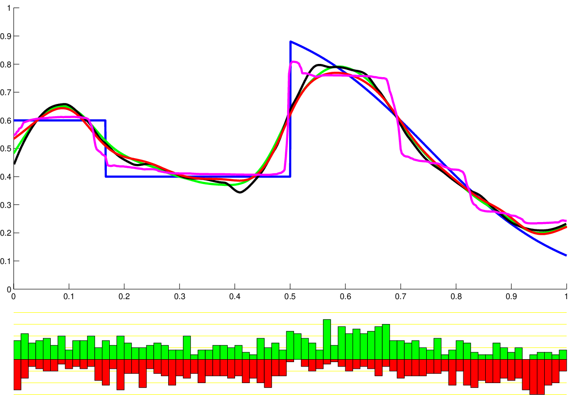
Key: True (blue), Posterior Mean (magenta), Loess (black), Smoothing Spline (green), Kernel Smoother (red)
Figure 4.2.b shows the results from running three standard smoothers. The results are little surprise. The three smoother’s estimates are quite similar over all on this example. They over-smooth the jumps, but partially make up for this by giving a smoother approximation on the smooth half. They also all take a turn at the ends; this is consistent with the data which happens to behave somewhat unusually there.
Loess (plotted in black) fits a locally-weighted linear regression at each point to make its estimate. Smoothing splines (in green) use efficient computational tricks to compute the regression curve that optimizes a tradeoff between small MSE and small integrated second derivative. Gaussian kernel smoothers (plotted in red) take a weighted average of response values near a point to predict. For each method, I chose a smoothing parameter that seemed to give results that were about as good as possible.
4.2.2 LARS/Lasso/Boosting

Key: True (blue), Posterior Mean (magenta), Lasso (Cp) (green)
The green curve in figure 4.2.d, shows the result of using a Lasso penalized regression. This was particularly easy to do using using the Least Angle Regression (LARS) software [30]. Like any linear regression, the results depend on what basis is chosen. For this example, the basis is constructed by considering the function for values of evenly spaced from to . To encode a datapoint with covariate under this basis, evaluate the functions at and pack the results into a vector: this vector becomes the covariate that the regression uses. Finally, Lasso regression resembles ordinary regression except for one critical difference: the regression parameter is penalized by , where is a tuning parameter. For this example, the parameter was chosen using a Cp criterion.
Constructed in this way, the Lasso regression estimate should be quite similar to the estimates that would be arrived at using other important techniques such as “Boosting stumps” and the least angle regression method. The similarity between these different methods is discussed in [30].
As can be seen from the figure, the Lasso estimate is has some appealing features. It is piecewise constant, but it also takes a fairly large number of steps and spaces them out usefully along the smooth transition on the right side of the figure. It does a reasonable jump of “detecting” the two change-points. On the other hand, it does not go as low as it should from to , nor as high as it should to the right of .
4.2.3 Wavelets

Key: True (blue), Posterior Mean (magenta), Wavelet 1 (green), Wavelet 2 (red), Wavelet 3 (black)
Figure 4.2.f compares some estimates that were based on wavelet techniques. The red, black, and dotted curves show various wavelet reconstructions of the regression curve. Overall, I think the results are quite disappointing; artifacts from the particular basis used show through clearly into the estimate. Since the data are not regularly spaced, some accommodation is necessary to use conventional software (e.g. Wavelab). Algorithms exist that apply directly to irregularly spaced data, but I did not successfully locate any working implementations. Instead, the dotted curve shows the wavelet reconstruction that results from simply using the ordered covariate values as if they were regularly spaced and then extrapolating back to the irregularly spaced reality.
There are a number of problems with this approach and some recent work has developed more sophisticated schemes. For the red and black curves, I tried one of the simplest [14] which recommends using direct linear interpolation to produce values on a fine grid and then applying wavelet shrinkage methods to this gridded data. The estimates were computed by the wden function in Matlab. It has a large number of options, most of which (quite frankly) I do not understand. These include the choice of a threshold selection rule from among four options, the choice to use hard or soft thresholding, an option titled “multiplicative threshold scaling” with three options, the choice of the level at which to compute the coefficients, and finally the name of the wavelet family to use (many options). For someone with as little experience with wavelet methods as me, these options are not a feature but a drawback. Furthermore, experimenting with the different options, they all seemed to make a difference. A reasonable, but not heroic effort was made to choose working parameter values. In any case, for the illustrated curves, the Matlab commands that were used are:
Xi=seq(min(X),max(X),2^12); % a fine grid of X-values
Yi=interp1(X,Y,Xi);         % on which to interpolate the response
Yhat1 = wden(Y, ’heursure’,’s’,’mln’, 8,’sym8’); % 1: green
Yhat2 = wden(Yi,’heursure’,’s’,’one’,10,’db4’ ); % 2: red
Yhat3 = wden(Yi,’heursure’,’s’,’one’,10,’haar’); % 3: black
4.3 Comparison with Dyadic Prior

For comparison, Figure 4.3.b shows the result of computing the posterior mean resulting from the Diaconis and Freedman dyadic binary regression prior [25]. Like the prior studied in this thesis, this prior chooses a random partition and assigns independent success probabilities to each partition element. However, this prior uses a dyadic partition, splitting the data into equal pieces for some . The consistency of the resulting estimates is guaranteed for any choice of hierarchy prior, except perhaps when the true regression function is identically and the data is pure noise. For this case, certain priors will be consistent and others will be inconsistent. It was of interest, then to try one on the boundary. For this reason the prior on hierarchy level that was used assigns: for . In fact, for this data, the results were stable over a wide range of choices of .
Since the prior is dyadic, it has no trouble at all nailing the split at ; of course, it does not have such good luck for the split at . The posterior strongly favors a model with around steps.
4.4 Dependence on the Parameter of the Geometric Prior

In this section, consider a departure from the hierarchy prior. Figure 4.4.b shows what the posterior mean estimate would be for the data from experimental run 1, if a prior is used on the number of steps . As usual, the true response curve is indicated in blue, and the posterior mean estimate for is drawn in magenta; the posterior means for other values of are also drawn. As can be seen in the figure, as ranges from small values (short tail prior, dotted black curve) to large values (long tail prior, solid black curve) there is not so much difference in the posterior mean estimate except that certain small bumps and wiggles that are suppressed for the small values become visible for the larger values. Indirectly, this experiment also provides a check on the stability of the Monte Carlo estimates of the posterior mean; it is unlikely that there would be such close agreement among these independently computed estimates if the MCMC was not working reasonably well. To make a more detailed comparison, it would be sensible to pool the sampled regression curves and use an importance sampling technique to compute combined results. I do not pursue this here.

It is also of interest to know how many splits the posterior is using. Figure 4.4.d shows the posterior on the number of steps for three hierarchy priors: , and respectively. The difference between the priors has a more pronounced effect here. Under a prior with , complex models are quite rare and consequently, the posterior on step size shown in the top panel has a fairly short tail. Notice, though, that even for this conservative model, the likelihood has been able to overwhelm the conservative prior enough to shift most of the posterior mass onto models with splits.
For the bottom panel, , which corresponds to a rather slowly decaying tail. Notice, though, that the tail of the posterior is not nearly this long: models with a large number of steps can fit the data well, but also have a large number of parameters: . This tends to down-weight them as a group. When the posterior is marginalized to yield the posterior distribution on the number of steps, an account is taken of “how many” of these more complicated models give a good fit as well as how good the fit itself is. Because of this trade of, models with steps are the most common.
The middle panel, corresponds to the prior that has been the subject of so many experiments. Notice that models with fewer than steps have almost no effect on the posterior mean; most of the mass is on models with to steps: is the most common choice.
4.5 The Predictive Probability Surface

To better understand the interaction of the data and the posterior on experimental run 1, reference to Figure 4.5.b is useful. It demonstrates just how spiky, multi-modal, and (in particular) non-normal the posterior’s density can be. It shows a slice of the posterior for the change-point case (i.e. four steps). One change-point is fixed at (not shown) because this was the most likely location for a single split; this location accounts for the jump at in . The other two change-points are allowed to range over the and axes of the plot. More technically, what is plotted is a self-normalized version of the function , defined by Equation 3.23 where . Essentially computes the likelihood that the splits occur at a given location; it marginalizes out the different possible choices for the success probabilities. The height of the surface follows , and the color follows , so that the small-probability structure is also visible. The and axes are symmetric, of course, because splitting at and is the same as splitting at and . Similarly the function is largest along horizontal and vertical “bands.” This is because when one split is in a particularly fortuitous place, it tends to improve the fit over all, even if the placement of the second split is suboptimal. The highest two peaks (near the opposite corners), represent splitting on the left (in the vicinity of ) to take care of the jump that is there, and on the right (in the vicinity of ) to split the smooth transition region into its higher and lower halves. The secondary peaks near the far corner, represent splitting the smooth transition in two places and ignoring the left half (recall that this was the choice made by CART on this data).
4.6 Behavior on a Small Data Set

It is interesting to see how the posterior responds to individual data points; this is most easily seen in a very small dataset. In Figure 4.6.b I consider a data set with 5 data points, that, as usual are shown by the two histograms. In this case there are two heads on the left and three tails on the right. The posterior mean (magenta) is seen to respond in a smooth way, except at the data points where it remains continuous but takes a (small) sharp turn. The other colored curves represent the posterior mean when the number of steps that the function is allowed to take is fixed a-priori. The flat black line, for example, is the posterior mean when no splits are allowed (one step). The red curve, on the other hand is the posterior mean if 14 splits (15 steps) are required. Notice how the red curve, especially, drifts back towards for -values that are not close to the data points. This happens because with 14 splits and 5 data points, there are bound to be many empty intervals and those, necessarily, fall back on the prior. The posterior mean curve for a prior on the number of steps is the weighted average of these curves, where the weights (as percentages) have been tabulated by the inset histogram. Since the -split model fits this data so especially well, it winds up contributing about as much as the contant model (which cannot be ruled out with so little data) to the final result. The contribution of the higher models is not forgotten, though; notice how the posterior mean (magenta) drifts back to slightly on the left of and the right of . Overall the posterior mean is conservative; it does not, for example, split the data in half at and declare the left hand mean to be and the right hand mean to be .
4.7 Behavior on a Large Data Set

Key: True (blue), Posterior Mean () (magenta), Posterior Mean () (green), CART (black), min-xerr CART (dashed black)
The data from experimental run 1, consisted of pairs with the -values drawn uniformly from and the -values drawn . This section answers the question: how does the posterior change if this data set is enlarged to have datapoints by generating additional data from this model? As usual the true curve is drawn in blue and the posterior mean for the prior is drawn in magenta. The data set, as is visible from the histograms, is getting rather large. Pleasantly, the posterior mean estimate is also giving an accurate estimate of the true curve. Somewhat disappointingly, though, the step functions on which the prior is based have not gone away. Although they are smaller, they are clearly visible in the magenta curve.
The CART estimate for this data is shown in black. A couple of observations need to be made. First of all, because the -standard-deviation pruning rule was used, the CART curve only has splits. Looking through the full tree, the model that minimizes the cross-validated error has two additional splits and is drawn by the dotted black line. This model agrees quite closely with the posterior mean estimate, but two of its splits were pruned away when the -standard-deviation pruning rule was used because the standard deviation of the xerr is not small enough. It might be selected automatically if a more intensive cross-validation were used. Finally, note that both CART curves minor artifacts (when compared to the posterior mean) that result from the greedy nature of the full tree.
One might suppose that with this much data, it ought to be possible to fit a model with many more steps. This does not seem to be true (at least for a prior that models the success probabilities independently). For example, if the full CART tree is manually pruned to have only one or two additional splits beyond the that were used by the minimum xerr model, the additional splits visibly degrade the fit. To understand this, consider that the right half of the data should contain around points. By chance, they will not be (quite) evenly distributed over this half but for simplicity suppose that these “” points are divided evenly into the intervals selected by the larger CART model. This leaves around points in each partition cell. Recall that the variance of a random variable is , so that the standard deviation of the estimated success probability on each of these partition cells is going to be around . Considering that the regression estimator has to not only detect a difference, but also locate a good choice of split, and optimize the accuracy of the estimated success probability, it does not seem too unreasonable that the average jump in success probability between neighboring cells is around .
Also shown (by the green curve) is the result of computing the posterior mean when a prior is used for . Interestingly, this long tail makes little difference and the green curve barely peaks out from under the magenta one.
4.8 The Effect of Sample Size


The previous section developed a extended version of experimental run 1 that contained data points. In figure 4.8.b, this data is analyzed in more detail. Smaller data sets are formed by taking the first data points for ranging from to by powers of two. It is very pleasant to see how the posterior mean incrementally grows closer to the truth. At first, the steps on the left are almost ignored (with so little data, any pattern they contain could have resulted from noise), but gradually they fill in. The transitions near the change-points in become very sharp and the estimates of the smooth transition steadily improve.
4.9 The Effect of Sample Size: a Harder Example


For the final example, I consider a much harder regression function. It is depicted in blue in Figure 4.9.b. It was formed by taking multiple copies of the original and shrinking them to half their size repeatedly. A data set with point is simulated and the posterior mean is calculated for subsets of increasing size. As had been hoped, the features get filled in as the data size increases incrementally. The larger features rise above the noise first and then the smaller, so that for this regression function, the approximation seems to grow better as increases on the right first, but then steadily spreads to the left. Importantly, for the larger , the posterior mean concentrates on models with many more splits than it did for the easier data since. Presumably this is because more complex models are necessary to increase the likelihood. To some extent this makes sense because even though this example is more complex than the previous one, some aspects of the regression function are relatively easy to detect (e.g. the large jump) and there are more of these features available for analysis. It is interesting to compare the results with the former dataset for with the results on the right half of the current dataset for . They should be quite comparable because the regression function for this more complicated model on is just a rescaled version of the original model, and in both cases there should be about datapoints available. To appearances, the two results are quite similar except that the latter result does not do as well on the small interval from to around . Perhaps it is being confused by the low success probability region immediately to the left of . Conducting a similar comparison between the original example the right half of the example, the latter result seems substantially inferior. On the other hand, it is not so bad when compared with the original result on experimental run 5. Furthermore, the performance of the posterior mean is quite good considering the overall increase in the difficulty of this problem. Even more amazing, considering the popular state-of-the-art methods, it does all of this without any tuning or cross-validation.
Chapter 5 Consistency
This chapter establishes conditions under which the prior for one-dimensional classification that was introduced in section 1.2 is a consistent estimator of the true regression function. The consistency of the posterior is proven using a result by Barron, Schervish, and Wasserman [2]. Before reviewing their theorem, I pause to introduce some notation. I also present a lemma that shows that the original conditions given in their theorem are equivalent to some others that may be easier to check. Finally, I specify the prior more formally and complete a proof of consistency.
5.1 Notation and the Basic Theorem
Let be the class of all (Borel) measurable functions . Write for the uniform distribution on and for counting measure on the set . Write for the product space , and call the product measure . To any there is a corresponding density on with respect to that we denote by :
| (5.1) |
For notational convenience, we may write either for and or for . Write for the distribution on whose density with respect to is . In words, the consequence of this construction is that sampling a point from is the same as choosing an uniformly on and then (conditionally on ) determining by flipping an “” coin.
Write for the class of densities formed by considering for every .
Let denote the Hellinger distance on :
| (5.2) |
And let denote the Kullback-Leibler discrepancy on (employing the usual convention that the integrand is interpreted as 0 whenever ):
| (5.3) |
We are concerned with posterior consistency and so the mass that the prior or posterior ascribes to certain small sets containing the true parameter is of interest. For any , we define two such “neighborhoods:”
| (5.4) | ||||
| (5.5) |
The “richness” of the parameter space is also an important quantity; to make this precise we supply the following definitions.
Definition 1.
Consider a class of functions that are densities with respect to dominating measure . We say that the collection of functions is a -upper bracketing of if:
- 1.
for every there exists such that a.e.
- 2.
every satisfies
Furthermore, write for the -upper metric entropy of which is the logarithm of the size of the smallest possible -upper bracketing of (infinity, if no finite bracketings exist).
The following result can now be stated. It gives conditions on the prior that are sufficient to ensure that the posterior will concentrate on for any .
Theorem 4 (Barron, Schervish, and Wasserman 1999).
Let be a -finite measure on a measurable space , where the -field is separable. Let be a probability distribution on , a class of probability densities with respect to . Endow with the Borel -field induced by the Hellinger metric . Let be a certain chosen density with respect to and write for the corresponding distribution on . Let be drawn from . In the notations explained above, further assume that for every :
- 1.
- 2.
There exists a sequence of measurable subsets of and positive, real numbers and such that:
- (a)
for all sufficiently large
- (b)
for all sufficiently large
- (c)
- (d)
- (a)
Then, with probability [under measure], Bayes theorem applies for all ; i.e. for any measurable and any :
And for any :
The second condition of this theorem seems rather technical. To restate this theorem in simpler terms we prove an elementary lemma which shows that these conditions (item I in the lemma) can be expressed in three other equivalent forms.
Lemma 5.
The following conditions, given in the notation defined above, are equivalent:
- I
For all , there exists , a sequence of measurable subsets of and positive, real numbers and such that:
- a
for all sufficiently large
- b
for all sufficiently large
- c
- d
- a
- II
There exists a sequence of positive real numbers , with , and , a sequence of sequences of measurable subsets of such that:
- a
for all ,
- b
- a
- III
For all there exists , a sequence of measurable subsets of and a positive, real number such that:
- a
- b
- a
- IV
For all there exists , a sequence of measurable subsets of such that:
- a
- b
- a
Proof.
I II:
First, notice that the condition from I.a that “there exist and so that for sufficiently large” implies that . Conversely, if , then for all sufficiently large , and for all sufficiently large .
Choose a sequence of , and use I to establish the existence of satisfying I for . Since , we can find a subsequence on which . Without loss of generality, assume we already have such a subsequence. The above reasoning, then, establishes II.a for this sequence. Since I.a implies that for all , to establish II.b, we need only show that . Condition I.c constrains . Viewing this as a function of , notice that it is monotonically decreasing on so that, necessarily, , the value of this function at .
II I:
Consider some . Note that as . Find an sufficiently large so that this expression is at least . Then find a subsequent sufficiently large so that Choose and , and I is proven.
II III: This is a straightforward exercise in nitpicking.
III IV: Observe from the definition that is a non-increasing function of .
∎
Theorem 6 (Corollary to Barron, Schervish, and Wasserman 1999).
Let be a -finite measure on a measurable space , where the -field is separable. Let be a probability distribution on , a class of probability densities with respect to . Endow with the Borel -field induced by the Hellinger metric . Let be a certain chosen density with respect to and write for the corresponding distribution on . Let be drawn from . In the notations explained above, further assume that for every :
- 1
There exists a sequence of measurable subsets of , so that:
- 2
- 3
Then, with probability [under measure], Bayes theorem applies for all ; i.e. for any measurable and any :
And for any :
In words, this is what we have required: 1) the prior must put positive mass on all Kullback-Leibler neighborhoods of . 2) We must be able to choose an increasing sequence of subsets of the parameter space so that the ’th of these sets captures all but exponentially much of the prior mass 3) This sequence must not grow in “complexity” too quickly. We conclude that the posterior will concentrate on the subset of the parameter space which is Hellinger close to the true parameter.
5.2 Specification of the Prior
We describe as a distribution on by means of first describing a parametric prior . Let be a distribution on the positive integers. Let and let . Let be the distribution on , that can be described by first picking according to ; and then, conditional on , picking a point uniformly from . That is, and are chosen independently and uniformly from the appropriate unit cubes. Let denote the ’th ordered value of . Now to any associate the function given by the following construction. For , let . If , just let . Take . Finally, then, to draw from , draw from , construct , and form as in Equation 5.1.
5.3 A Consistency Proof
This section proves that the prior just described is consistent in the sense that, under repeated sampling, the posterior mass will concentrate on a Hellinger neighborhood for any . The proof uses three lemmas to establish the conditions of Theorem 6.
The first lemma shows that puts mass on all Kullback-Leibler neighborhoods .
Lemma 7.
Let be the prior distribution on , the class of densities w.r.t , that was described above. Assume that , the hierarchy prior, assigns positive mass to every natural number. Let be an arbitrary density in . Then, for any , .
Proof.
Let be the corresponding function in . For some , to be determined later, let:
Let where . By Chebyshev’s inequality, for any , the Lebesgue measure of is smaller than .

In other words, as shown in Figure 5.3.b, if , this restricts the pair to lie in the convex set (blue) whose extreme points are , , , . For , we still have a restriction on , so that the pair lies in the rectangle (green) with vertices , , , . Let denote the Kullback-Leibler discrepancy between the and distributions.
Then for any we can bound , as follows:
| (5.6) | ||||
| (5.7) | ||||
| and because is convex in the pair [13], the supremum is achieved at the vertices so that the above is bounded by: | ||||
| (5.8) | ||||
| Using the symmetry | ||||
| (5.9) | ||||
| (5.10) | ||||
| (5.11) | ||||
| For small , the last term is the most important. To simplify the first term, verify that for , | ||||
| (5.12) | ||||
| (5.13) | ||||
| (5.14) | ||||
Which tends to zero as . For a sufficiently small choice of , then:
It remains to show that has positive prior mass. To do this, we first find a step function which approximates and then show that , a set of perturbations of , remains in and that has positive prior mass.
Observe that since is Lebesgue-measurable there exist two increasing sequences of step functions and for which . This is, in fact, the basis of a common construction of the Lebesgue integral [42]. Consequently, we can find a step function for which . Let be the function obtained by modifying so that it always remains in , i.e. , so that and .
Now, parameterize in the manner of section 5.2 (changing it at a set of measure 0 if necessary) so that is the number of locally constant regions in and the vectors and signify the change-points and success probabilities of .
If we then perturb each towards the value by no more than we obtain a new function which remains in and satisfies . If, in addition, we perturb the ’s by no more than we obtain which also remains in , satisfying or .
Denote the class of functions thus obtained by . Then . ∎
Remark 1.
A shorter proof can be based on the martingale sequence formed from conditional expectations of .
For the second lemma, consider , the class of functions which are constant except possibly for as many as change-points.
Definition 2.
Using the notation from section 5.2, let . Let be the associated class of densities with respect to :
Lemma 8.
The -upper bracketing entropy of the class is no more than .
Proof.
Fix positive integers. Partition into equal intervals . Consider the class of all functions that can be formed in the following way: Choose some of these intervals. Let be the union of the chosen intervals and let be the nonempty subintervals of formed by subtracting (). Finally choose . Construct the function by:
It is easy to see that, by appropriate choices, for any we can find an that is greater than or equal to it globally. Furthermore, the integral of is less than or equal to . The size of is . By choosing , we have shown that . ∎
The final lemma establishes a result about the tail of random variables.
Lemma 9.
If for some , then for any :
And, consequently, for any there is a sufficiently large so that for every , .
Proof.
Now, the bracketed term is no more than 1 and we are left with a geometric series whose factor, is less than by our assumption so that:
So that for sufficiently large, from Stirling’s formula:
∎
The main result can now be established.
Theorem 10.
Suppose that the prior , described in section 5.2 is based on the hierarchy prior . Suppose that gives positive probability to every natural number and that its tail satisfies: for all sufficiently large and some . Let be an arbitrary measurable function from into . Suppose that are drawn from the distribution , which has density with respect to . Equivalently, suppose that the ’s () are drawn as follows: the ’s are drawn independently and uniformly from ; and, conditional on , is an independent random variable. Then, in the notation of section 5.1, for any , as [-a.s.]. Specifically, for any , and any , the posterior mass on the set tends to as [-a.s.].
Proof.
Let . Choose the sequence as . Then, by Lemma 8, . Observe that as . For large enough, then:
Choosing , we have proven that .
Now calculate that for all sufficiently large ,
Consequently, .
The statement about follows from the equivalence of the and Hellinger metrics for bounded densities. This fact and other useful inequalities about Hellinger distance (aka Jeffrey’s distance) are reviewed in [22, section 5.8 and excercise 5.7] which states:
| (5.15) |
Finally, the equivalence of the -norm and the norm for and for all densities uniformly bounded by a constant, is well known. ∎
Remark 2.
Applying Lemma 9 shows that the preceding theorem applies to any hierarchy prior whose tail behaves like that of a , for any . The theorem does not apply to the case in which is .
Remark 3.
The restrictions on the tail of the prior occur because condition 3 in Theorem 6 requires that the “sieve” sets do not grow in “size” too quickly as grows. The choice made in the proof of this theorem is (essentially) the fastest rate of growth that this situation permits (in the absence of better bracketing estimates). Accordingly, condition 2 of Theorem 6 requires that the tail of the prior drops off somewhat faster than a distribution.
Remark 4.
For further discussion of how to interpret this result, please see the discussion in chapter 6.
Chapter 6 Discussion of Consistency Results
It is challenging to suggest what the practical consequences (if any) of Theorem 10 are. It proves that under the modeling set up with iid observations that has been considered throughout this thesis, that the posterior of the random split prior is a consistent estimate of any measurable true regression function if the tail of the prior decays at least as fast as for some . Perhaps it would be wise not to over interpret the result. After all, it only supplies a sufficient condition for consistency and does not either establish that priors lead to inconsistent estimators or that -like priors are a good (i.e. practical) idea. Additionally, it attempts to prove consistency in a fairly strong sense: that the posterior mass concentrates on Hellinger neighborhoods of the truth. Weaker consistency results, say that the posterior mean be consistent, might go through under milder assumptions.
6.1 Consideration of the Diaconis and Freedman Results
Judging from the results of Diaconis and Freedman for their prior, as discussed in subsection 2.2.1, it might, in fact, be the case that the posterior is consistent for any hierarchy prior (with full support), so long as is not the constant function . That is, it might be that the only situation in which is inconsistent (even using a “poor” choice of ) is when there is no real pattern at all in the data because every coin flip was fair. Note that if this were our only concern, namely that the estimates might be inconsistent under some specific finite collection of possible scenarios, this could be easily addressed (albeit in a decidedly non-Bayesian way), by choosing a prior that puts point mass on the troublesome cases. Consistency for these exceptions would then be guaranteed by a suitable application of Doob’s result [29]. Interestingly, it could destroy consistency for other cases. An example of such a mixture is given by Diaconis and Freedman [31]. Of course, a true subjective Bayesian would never change his or her prior in this way. Rather, unless these cases actually are a subjective impossibility, a purist would merely see this as an explication of why their true prior (that they are perhaps still in the process of articulating) differs from the former one.
6.2 An Experiment to Check a Worrisome Case
It seems reasonable to try and test for the possibility of inconsistency when the true function by running a simulation experiment. To do this, generate an increasing sequence of data sets over a range of sizes that are drawn from the distribution. That is, since there is no true signal at all in the data, it will be interesting to see how the posterior mean responds. For a prior, the posterior mean should (at least eventually) settle down, but will this hold for a prior? Indeed, the results in figures 6.2.b, and 6.2.d indicate that both estimates correctly identify the null case, whether using a prior or a one respectively. A new feature of these figures is the small histogram included on each one. It is a histogram of the posterior on the number of steps in the unknown function. The prior starts out believing that there will be a good number of steps in the data. This is clearly reflected in the histograms in Figure 6.2.b for and . The posterior mean in these cases has more “wiggle” than for the prior even though both estimates see the same data. For both estimates find that the posterior mean is roughly constant, but somewhat lower than . Apparently, this is a real feature of the data and not an artifact of either prior. Eventually, for large all of these minor considerations wash out and clear preference for very flat models has triumphed. Interestingly, from or so onwards, looking at the histogram of , the prior has become convinced that the model has only one split. The prior is only beginning to reach this level of certainty about the truth as reaches .


6.3 Theory versus Practice
Nevertheless, if the user insists upon using an estimation procedure that has been proven to be consistent (say, by the preceding theorem), he or she still have a great deal of freedom. Roughly speaking, they can use any hierarchy prior they like on the first natural numbers and append to it an arbitrary tail. It is hard to imagine that there would be any practical difference between the estimators resulting from this “extended” prior and those resulting from the unmodified one, at least for realistic sample sizes. There certainly would not be any difference in practice, because in practice we only approximately compute the posterior anyway and no ordinary Markov chain Monte Carlo would ever be run long enough to notice the change.
6.4 Heuristics about Poisson and Geometric Priors
Despite these concerns, I still (tentatively) advocate the use of a prior because of the following heuristic arguments: (a) it favors simple models (b) its tail does not drop off “too quickly” so that it will hopefully not require enormous amounts of evidence for the data to “overwhelm” the prior: by ruling out simple models in favor of better fitting models (c) its tail does drop steadily; hopefully this will protect us from “over-fitting” (d) if we consider the mode of the posterior (on a log scale), the geometric prior penalizes each additional split by a constant () so that for the mode to shift to a model with an additional split we require a commensurate improvement in the log-likelihood of the data.
If using a prior, I would be concerned that I might have specified a parameter that was too small. If the true regression function were unexpectedly complicated, it might take a large amount of data to overwhelm the prior. Interestingly, if we attempt to remedy this by taking an exponential mixture of ’s, we get back a prior.
Another objection of mine is that (for modestly large ) the prior puts less mass on models with one region than on models with two regions. This makes sense if I actually expect that the regression function will be fairly complicated, but it violates my (frequentist) training to consider a complex model before “eliminating” the simpler one.
As a compromise I would propose a prior on that was until a certain point and then decays like a . On the other hand, if, in fact, priors prove reliable or even conservative, it might make sense to consider an even heavier tailed distribution. A modest proposal is to take a uniform mixture of priors for ranging from to . This results in a prior whose tail decays like , the mass at being .
6.5 Conclusions
None of these arguments is conclusive. In the absence of sound theoretical arguments it is perhaps best to rely on experimental evidence. From chapter 4 there is a good bit of evidence that priors perform well. What do priors do when applied to these data sets? In Figure 6.5.b the posterior mean resulting from a prior for three values of is plotted. The results are comparable to what happened as was varied in Figure 4.4.b. The prior with the shorter tail flattens out some bumps that the prior with the longer tail leaves in.

Key: True (blue), prior (cyan), prior (black), prior (green)
Still, for some applications especially, the practical question remains: how to choose (respectively )? Experience in the problem domain is the only method I can readily propose. Alternatives, like using cross-validation or an empirical Bayes approach remain attractive, but unproven.
Chapter 7 Extensions
There are numerous ways in which to extend , but perhaps the most pressing is to extend to multi-dimensional data sets where the predictor is in . One route to extend to higher dimensional problems is to observe that basically, all we need to consider is a suitable way to partition the space randomly. If an interesting way to choose a partition at random is found, then describe a new prior by saying: draw a partition and give each region an independent uniform success probability. One natural way to randomly partition is to suppose that a certain number of generating points are drawn from a Poisson process with constant rate function and to associate each point with its Voronoi (nearest neighbor) region. Alternatively, one could select a subset of the observed -values at random and use their locations to determine a Voronoi partition. This alternative is, unfortunately, not a purely Bayesian proposal since the partitioning depends on the data set given. On the other hand, it only depends on the -values of the data set, so that it remains a Bayesian procedure with respect to the response data (the -values).
To be specific, the prior I consider (call it ) can be described by the following. Let denote the observed values of the covariates in and let be a metric on . Proper choice of is essential to good performance in complex applications, but using Euclidean distance should suffice for simple problems. To any subset of the full list associate the Voronoi partition of . That is, say that a point is in the cell if for . For definiteness, in the case of ties say that is in the cell occurring first in the original ordering of the ’s. Consequently, every point is in exactly one cell. Put a prior on these partitions of the space by putting a prior on the (finite) set of all possible (nonempty) subsets of the list . Say that the prior probability of a subset only depends on the size of the subset and that the probability of a given size , is proportional to the probability that a random variable takes the value . Finally, having chosen a subset at random, and consequently having fixed a partition of , assign to each element of the partition a success probability drawn uniformly at random from . The generates a multi-dimensional regression function at random.

To explore these ideas I simulated a two dimensional data set with 250 data points, illustrated in Figure 7.0.b. The -values were chosen randomly (albeit not uniformly) from the illustrated rectangle; the -values were drawn as independent random variables whose success probability is indicated by the gray-scale in the figure. Points in the whiter regions have a higher chance of being an “x,” (i.e. ) while points in the darker regions have a higher chance of being an “o” (i.e. ). Jointly, the and data was actually generated in my simulation in the reverse manner: a fair coin was flipped to determine if will be or and then (conditionally) an -value was chosen. Suppose came up as , then with probability , will be drawn uniformly from the square on the right; otherwise, with probability it will be drawn from a bivariate normal distribution with standard deviation that is centered on the left-hand square. If came up a , the situation for would be reversed. These two descriptions are essentially equivalent and the goal for the posterior mean estimate is always the same: to estimate the conditional probability of to be given ; i.e. to estimate the gray-scale image.
Sampling from the posterior of this prior is (theoretically at least) quite simple. As before in chapter 3, the success probabilities can be integrated out analytically so that the posterior probability of a particular (nonempty) subset of size is proportional to:
| (7.1) |
Where and denote the number of -values equal to or , respectively, on partition element . Conditionally, the posterior distribution of a certain success probability is . Since the number of possible subsets is finite and all of them (except the empty subset) have positive posterior probability, a standard Metropolis-Hastings type MCMC allows us to sample from the posterior (at least in theory). In practice, though, the rate of mixing matters; in an effort to improve this I have conducted preliminary work that employs the simulated tempering technique developed by Geyer and Thompson [39].
All that remains to be specified is a transitive random-walk on (nonempty) subsets of a set of elements which has a known stationary distribution. This is easily done. Identify the class of all subsets of a set of size with the class of binary vector of length , with each coordinate indicating the presence or absence of a given element. Exclude the -vector from this set. Consider the random walk that picks a number randomly from to and then proposes flipping the ’th bit. The proposal is not allowed if it would create the -vector; hold in this case. This Markov chain is easily seen to sample uniformly from the class of all non-empty subsets and consequently it is easy to modify it with the Metropolis-Hastings ratio in order to sample from the posterior.

Sample 1

Sample 2

Sample 3

Sample 4

Sample 5

Sample 6


I have also proposed extensions of this technique to put a prior on smooth functions; under this proposal the prior concentrates on functions which softly partition the space using weighted Voronoi regions, but provide for smooth transitions between regions.
A simple extension of this technique that removes many of the artifacts that are otherwise present because of the dependence on the particular locations of the covariates can be made by using a randomly weighted Voronoi partitions [54]. To make such a prior, simply augment each cell with a random variable which is an independent a priori. Then, redefine the Voronoi partition so that cells with higher weight tend to be bigger. Specifically, consider the point to be in cell rather than cell whenever: . Intuitively, if an ordinary Voronoi partition can be understood by supposing that “crystals” grow out radially from the generating seeds until they hit other growing crystals, then this weighted Voronoi partition allows for the crystals to grow at different rates. It is also simple to allow the crystals to start growing at different times (by simply adding a different random offset to for each cell). The overall scale of the prior on is irrelevant so this parameterization sets the mean to . For the experiment shown in Figure 7.0.h I used . As can be seen, this simple modification allows the posterior to choose neat balls and lines with which to isolate out the different contours of the data. The posterior is computed using standard MCMC techniques.
Another route to extend is to utilize the observed connection between and (for details, please refer to subsection 2.2.1). To make that connection, I employed binary random variables that indicated if a test point was or was not above a certain random threshold . To generalize, then, we can take to indicate if is in a certain random half-space . This would be similar to a version of CART in which we split first into two halves via , and then split each half via , and so on. We could make something close to ordinary CART if we utilized random coordinate aligned half-spaces and if we employed a suitably “regularized” which did not assign an independent uniform to all possible binary -tuples at level . More generally, one can invent other ways of “regularizing” so that numerous binary tuples are tied together.

Finally, for comparison, Figure 7.0.j the result of bagging ordinary two-dimensional CART on this same data is shown. It has a clear advantage on the vertical split down the center that happens to be coordinate aligned. It does a decent job of isolating the two clumps of data. Interestingly, there is a clear horizontal and vertical blurring pattern that arises from the use of partitions that only partially isolated the clumped data: it is isolated in one coordinate, but not in the other.
Chapter 8 Afterword
As statisticians, we analyze data, formulate models, estimate parameters, and use these models to form predictions about future data. Broadly speaking, then, our business is inference. We go to a lot of trouble to formulate good models and we have spent a great deal of effort debating about the details of how to make inference within a model – e.g. Bayesian versus frequentist inference.
Generally, though, the way we select our model remains an art. “Non-parametric” methods are a step forward here, because, generally speaking, they at least prescribe how to select a variety of “smoothing-parameters” which essentially determine which model among some class of models we actually apply. The main topic of this thesis is of this sort: A Bayesian approach to the question of how to estimate the number and location of change-points or, more generally, how to choose a partition of the data into approximately exchangeable subsets.
In this afterword, I would like to step back from the details of this subject and address the more general problem of how we formulate a model. Sometimes, we prefer to shunt responsibility for this and appeal to the scientist for help; but, fundamentally, all inference comes back to data eventually – how else did the scientists discover their model? Considering, then, that the formulation of a model is essentially “an art,” and that we know that the results of our analyses are not absolute, but relative to the modeling choices we have made, how can we be so bold as to expect that reality will conform to our model-specific “confidence intervals?” This is not to say that statistical practice does not work, or that the formal properties of our analyses under our stated assumptions are invalid, but simply to remind the reader that the thread that connects the prescribed model with reality has no formal basis.
In practice, a good rule of thumb is to consider several models and, consciously or not, select one which is simple and which we expect will fit the data at least nearly as well as other more complicated models that we might prefer not to have to consider. In practice, we look at the data ourselves before selecting a model and build in any particular types of regularity that we happen to notice that it possesses into our model – at least if we think it will affect our conclusions.
Bayesian analysts do not escape these problems. They may subjectively allow for a mixture of several different models and for a range of “hyper-parameters” but this only ameliorates the core problem because no-one ever accounts for all the possible regularities that might be found.
To further make my point, consider the following, admittedly fanciful, thought experiment. An alien race comes to earth and challenges mankind to an intelligence test. We are given a binary time-series to analyze one-hundred bits at a time. It begins innocuously enough:
     01000001000000100000110111101110000000100101000011
     10101010000000001110010010000000001011001101101010
What statistical models shall we consider? We could try Bernoulli, or perhaps a hidden Markov model. If ambitious, we might let the data choose the order of our model. Upon doing so, we find that the null model fits best, despite the superficial appearance of runs, and we model the data as random coins with success probability . The aliens ask us to give a confidence interval on the fraction of ’s in the next 100 bits and to estimate the probability that the 50’th bit of this new data will be 1. Most statisticians fall back on the classics and use something approximately like for both answers. Others who used a richer model suggest wider intervals and the ordinary debate ensues.
So far so good, right? Or should we worry that our glance at the data and default choice of classical model may miss structure that we failed to notice? Naah! The aliens couldn’t be that tricky…. Then the next 100 bits arrive.
     00000000000000000000000000000000000000000000000000
     00000000000000000000000000000000000000000000000000
A dramatic failure, but no problem, the advocates of the HMM model were ready for this sort of thing. We have, they argue, simply encountered a hidden state which always produces 0. This explains the data well enough, but some remain skeptical. They propose that the character of the data may change with every new segment of 100 bits so that the effective size of our data set is only 2. The next 100 bits arrive.
     00011100011100011100011100011100011100011100011100
     01110001110001110001110001110001110001110001110001
And again we are surprised. Some HMM advocates insist we just need to add a number of new hidden states. Others extend the HMM model to favor this sort of cycle-like behavior. The next 100 bits arrive.
     00100100001111110110101010001000100001011010001100
     00100011010011000100110001100110001010001011100000
And most are satisfied that the data has returned to , but with the world attention that this situation has generated someone notices that these are, in fact, the first 100 bits in the expansion for the fractional part of . (C.f. http://www.algonet.se/~eliasb/pi/binpi.html) Oh dear – we certainly hadn’t planned on this – but we ignore this regularity in the data at our peril. It couldn’t happen by chance, could it?
As the test continues, we continue to be surprised by the patterns we are sent. By now, we have learned a lot: we know less than we think about the future. Every 100 bits we have been presented with a pattern that we hadn’t expected. Finally, we are given sequence after sequence that we can’t explain. Eventually the aliens conclude that, however feebly, we are, at least, a modestly intelligent form of life; and, taking pity on us, they decide to reveal the patterns we hadn’t discovered. The last sequences, for example, were actually Shakespeare, encoded by simple alien cipher that no human had ever considered. Furthermore, the first sequence wasn’t actually “random:” to generate it, all we had to do was start matlab or an equivalent (alien) computational program and type:
                x=rand(1,100)<=0.397;
                sprintf(’%c’,x+’0’)
Perhaps you object to my example. You prefer regression to time-series analysis and are content to consider data for which no-one would object to the model that the responses are independent given the predictors. Perhaps the problem of extrapolating a non-stationary time-series seems far too lofty to you. But you haven’t escaped it by wishing it away; in fact, the time-series problem can be embedded in the regression problem. We need only suppose that the covariates are tested one by one in some fixed designed fashion so that we see the responses sequentially. If we know that the regression function “smoothly” depends on the covariates, present methods can be expected to work; but, if the dependence is sufficiently complicated, each new data point tells us something entirely new, just like in my fictitious time-series.
Even if the data is generated – the regression case considered in most of my theoretical work – there is plenty of room for improvement. In this situation, we are, indeed, much better off – we can make rigorous probability statements about the quality of our predictions on average. Even so, as more and more data come in, and the general shape of the regression function becomes more tightly resolved, the “knowledge we gain” itself comes to us in a time-series fashion. Because of this, we cannot easily make predictions about the regression function at some fixed point.
For example, suppose the unit interval were divided into subintervals of size , , , etc… and suppose that the regression function takes a different value on each piece. In this way, we would quickly have enough data to estimate large-scale features, like the value of the regression function on the larger pieces, but if we are asked to make a prediction on one of the very small pieces, what are we to do? Perhaps, if we were smart enough, we wouldn’t blithely approximate the regression function as “smooth,” we would look for patterns in the regression values on the large pieces to help extrapolate to the smaller pieces. If, in fact, the regression values were seen to alternate between high and low, we would be silly to treat the function as “smooth.” Instead, let us hope that were are lucky enough that it is quite “regular.”
What, then are we to do? Consider again the alien’s test, and the complex sequence of modeling decisions that we needed to make along the way. How can we summarize the thought process that we went through as surprising data continued to come in? What possible prior on models could our analysis (even approximately) conform to? Our only recourse, it seems, is to formalize the idea of regularity and make explicit the manner in which we choose a model to accord with the regularities apparent in the data.
A reasonable defining property of regularity is that a distribution is regular if it can be (approximately) reproduced within a certain budget of time by applying some modestly short computer program to the data that we have previously seen and a “random sequence.” Roughly speaking, then, we can put a prior on models and/or regularities by putting a suitable prior on computer programs. Alternatively, we can select among the computer programs in a manner conforming more closely to the “method of maximum likelihood.” Formal versions of these ideas have been proposed [27],[63],[5],[47],[46],[13],[60] though much work is needed to formulate methods that are ready for actual use. Still, it seems to this author that the further development of some version of these ideas is an essential, natural, and unavoidable step in the progression of statistical thinking.
References
- Athreya et al. [1996] Athreya, K. B., Doss, H. and Sethuraman, J. (1996). On the convergence of the Markov chain simulation method. The Annals of Statistics 24 69–100.
- Barron et al. [1999] Barron, A., Schervish, M. J. and Wasserman, L. (1999). The consistency of posterior distributions in nonparametric problems. The Annals of Statistics 27 536–561.
- Breiman [1996]
Breiman, L. (1996).
Bagging predictors.
Machine Learning 24 123–140.
URL citeseer.nj.nec.com/breiman94bagging.html - Brieman et al. [1984] Brieman, L., Friedman, J., Olshen, R. and Stone, C. (1984). Classification and Regression Trees. Wadsworth.
- Chaitin [1966] Chaitin, G. J. (1966). On the length of programs for computing binary sequences. J. Assoc. Comp. Mach. 13 547–569.
- Chipman et al. [1998a] Chipman, H., George, E. I. and McCulloch, R. (1998a). Bayesian CART model search (with discussion). J. Amer. Statist. Assoc. 93 935–960.
- Chipman et al. [1998b] Chipman, H., George, E. I. and McCulloch, R. (1998b). Making sense of a forest of trees. Tech. rep., Department of Statistics and Actuarial Science, University of Waterloo.
- Chipman et al. [2000a] Chipman, H., George, E. I. and McCulloch, R. (2000a). Bayesian treed models. Tech. rep., Department of Statistics, University of Waterloo.
- Chipman et al. [2000b] Chipman, H., George, E. I. and McCulloch, R. (2000b). Hierarchical priors for Bayesian CART shrinkage. Statist. Comp. 10 17–24.
- Cleveland and Loader [1996] Cleveland, W. S. and Loader, C. (1996). Smoothing by local regression: Principles and methods (disc: P80-127). In Statistical Theory and Computational Aspects of Smoothing. Proceedings of the COMPSTAT ’94 Satellite Meeting.
- Coram [2001] Coram, M. (2001). Projection pursuit for classification: A different motivation for svms. Available upon request.
- Cover and Hart [1967] Cover, T. and Hart, P. (1967). Nearest neighbor pattern classification. Proc. IEEE Trans. Inform. Theory IT-11 21–27.
- Cover and Thomas [1991] Cover, T. M. and Thomas, J. A. (1991). Elements of Information Theory. Wiley.
- Daubechies et al. [1999] Daubechies, I., Guskov, I., Schroder, P. and Sweldens, W. (1999). Wavelets on irregular point sets. Phil. Trans. Royal Soc. Lond. A 257 2397–2413.
- Denison et al. [2002a] Denison, D., Adams, N., Holmes, C. and Hand, D. (2002a). Bayesian partition modelling. Comp. Statist. Data Anal. 38 475–485.
- Denison et al. [2002b] Denison, D., Holmes, C., Mallick, B. and Smith, A. (2002b). Bayesian Methods for Nonlinear Classification and Regression. Wiley.
- Denison et al. [1998a] Denison, D., Mallick, B. and Smith, A. (1998a). Automatic Bayesian curve fitting. J. Roy. Statist. Soc. B 60 333–350.
- Denison et al. [1998b] Denison, D., Mallick, B. and Smith, A. (1998b). A Bayesian CART algorithm. Biometrika 85 363–377.
- Denison et al. [1998c] Denison, D., Mallick, B. and Smith, A. (1998c). Bayesian MARS. Statist. Comp. 8 337–346.
- Denison [1997] Denison, D. G. T. (1997). Simulation based Bayesian nonparametric regression methods. Ph.D. thesis, Department of Mathematics, Imperial College, London.
- Devroye et al. [1996] Devroye, L., Gyorfi, L. and Lugosi, G. (1996). A Probabilistic Theory of Pattern Recognition. Springer-Verlag.
- Devroye and Lugosi [2001] Devroye, L. and Lugosi, G. (2001). Combinatorial Methods in Density Estimation. Springer.
- Diaconis and Freedman [1986] Diaconis, P. and Freedman, D. (1986). On the consistency of Bayes estimates (c/r: P26-67). The Annals of Statistics 14 1–26.
- Diaconis and Freedman [1993] Diaconis, P. and Freedman, D. A. (1993). Nonparametric binary regression: A Bayesian approach. The Annals of Statistics 21 2108–2137.
- Diaconis and Freedman [1995] Diaconis, P. and Freedman, D. A. (1995). Nonparametric binary regression with random covariates. Probability and Mathematical Statistics 15 243–273.
- Donoho and Johnstone [1994] Donoho, D. and Johnstone, I. (1994). Ideal spatial adaptation by wavelet shrinkage. Biometrika 81 425–455.
- Donoho [2002] Donoho, D. L. (2002). The Kolmogorov sampler. Tech. rep., Stanford University.
- Doob [1953] Doob, J. (1953). Stochastic Processes. Wiley.
- Doob [1949] Doob, J. L. (1949). Application of the theory of martingales. Colloque International Ctrenat. Rech. Sci, Paris.
- Efron et al. [2002] Efron, B., Hastie, T., Johnstone, I. and Tibshirani, R. (2002). Least angle regression. Tech. rep., Stanford University.
- Freedman and Diaconis [1984] Freedman, D. and Diaconis, P. (1984). On inconsistent bayes estimates in the discrete case. The Annals of Statistics 11 1109–1118.
- Freedman [1963] Freedman, D. A. (1963). On the asymptotic behavior of bayes’ estimates in the discrete case. Annals of Mathematical Statistics 34 1386–1403.
- Freedman [1999] Freedman, D. A. (1999). On the bernstein-von mises theorem with infinite-dimensional parameters. Annals of Statistics 27 1119–1140.
- Freund and Schapire [1996] Freund, Y. and Schapire, R. (1996). Machine Learning: Proceedings of the Thirteenth International Conference, chap. Experiments with a new boosting algorithm. Morgan Kauffman.
- Friedman [1991] Friedman, J. (1991). Multivariate adaptive regression splines. The Annals of Statistics 19.
- Friedman [1996] Friedman, J. (1996). On bias, variance, 0/1-loss, and the curse-of-dimensionality. Tech. rep., Stanford University.
- Geyer [1999] Geyer, C. (1999). Stochastic Geometry: Likelihood and Computation, chap. Likelihood Inference for Spatial Point Processes. Wiley, 79–140.
- Geyer and Moller [1994] Geyer, C. and Moller, J. (1994). Simulation procedures and likelihood inference for spatial point processes. Scandinavian Journal of Statistics 21 359–373.
- Geyer and Thompson [1993] Geyer, C. and Thompson, E. (1993). Annealing marko chain monte carlo with applications to ancestral inference. Tech. rep., University of Minnesota, School of Statistics.
- Ghosal et al. [2000] Ghosal, S., Ghosh, J. and van der Vaart, A. (2000). Convergence rates of posterior distributions. The Annals of Statistics 28 500–531.
- Green [1995] Green, P. J. (1995). Reversible jump markov chain monte carlo computation and bayesian model determination. Biometrika 82 711–732.
- Hasser and Sullivan [1971] Hasser, N. B. and Sullivan, J. A. (1971). Real Analysis. Dover.
- Hastie et al. [2001] Hastie, T., Tibshirani, R. and Friedman, J. (2001). The Elements of Statistical Learning. Springer-Verlag.
- Hastings [1970] Hastings, W. (1970). Monte carlo sampling methods using markov chains and their applications. Biometrika 57 97 – 109.
- Kendall and Møller [2000] Kendall, W. and Møller, J. (2000). Perfect simulation using dominating processes on ordered spaces, with application to stable point processes. Adv. Appl. Prob. 32 844–865.
- Kolmogorov [1965] Kolmogorov, A. N. (1965). Three approaches to the quantitative definition of information. Problems of Information Transmission 1 4–7.
- Kolmogorov [1968] Kolmogorov, A. N. (1968). Logical basis for information theory and probability theory. IEEE Trans. Inform. Theory IT-14 662–664.
- Lavine [1992] Lavine, M. (1992). Some aspects of polya tree distributions for statistical modelling. The Annals of Statistics 20 1222–1235.
- LeCam and Yang [1990] LeCam, L. M. and Yang, G. L. (1990). Asymptotics in Statistics: Some Basic Concepts. Springer.
- Liu [2001] Liu, J. (2001). Monte Carlo Strategies in Scientific Computing. Springer-Verlag.
- Metropolis et al. [1953] Metropolis, n., Rosenbluth, A., Rosenbluth, M., Teller, M. and Teller, E. (1953). Equations of state calculations by fast computing machines. J. Chem. Phys. 21 1087–1092.
- Møller [1999] Møller, J. (1999). Stochastic Geometry: Likelihood and Computation, chap. Markov Chain Monte Carlo and Spation Point Processes. Wiley, 141–172.
- Møller and Skare [2001]
Møller, J. and Skare, Ø. (2001).
Bayesian image analysis with coloured voronoi tessellations and a
view to applications in reservoir modelling.
URL citeseer.nj.nec.com/405679.html - Okabe et al. [1992] Okabe, A., Boots, B. and Sugihara, K. (1992). Spatial Tesselations: Concepts and Applications of Voronoi Diagrams. John Wiley & Sons.
- Paddock [1999] Paddock, S. (1999). Randomized Polya Trees: Bayesian Nonparametrics for Multivariate Data Analysis. Ph.D. thesis, Duke University.
- Ripley [1996] Ripley, B. (1996). Pattern Recognition and Neural Networks. Cambridge University Press.
- Rubin [1981] Rubin, D. B. (1981). The bayesian bootstrap. The Annals of Statistics 9 130–134.
- Scargle [1998] Scargle, J. (1998). Studies in astronomical time series analysis. v. bayesian blocks, a new method to analyze structure in photon counting data. The Annals of Statistics 504 405.
- Scargle et al. [2002] Scargle, J. et al. (2002). Private communication.
- Schmidhuber [2000] Schmidhuber, J. (2000). Algorithmic theories of everything. Tech. rep., IDSIA-20-00.
- Schwartz [1965] Schwartz, L. (1965). On Bayes procedures. Zeitschrift für Wahrscheinlichkeitstheorie und Verwandte Gebiete 4 10–26.
- Shen and Wasserman [2001] Shen, X. and Wasserman, L. (2001). Rates of convergence of posterior distributions. The Annals of Statistics 29.
- Solomonoff [1964] Solomonoff, R. J. (1964). A formal theory of inductive inference. Inform. Contr. 7 1–22, 224–254.
- Tierney [1994] Tierney, L. (1994). Markov chains for exploring posterior distributions. The Annals of Statistics 22 1701–1762.
- Vapnik [1996] Vapnik, V. (1996). The Nature of Statistical Learning Theory. Springer-Verlag.
- Wahba [1990] Wahba, G. (1990). Spline Models for Observational Data. SIAM.
- Wahba et al. [2000] Wahba, G., Li, Y. and Zhang, H. (2000). Advances in Large Margin Classifiers, chap. GACV for Support Vector Machines. MIT Press.
- Wong and Shen [1995] Wong, W. H. and Shen, X. (1995). Probability inequalities for likelihood ratios and convergence rates of sieve Mles. The Annals of Statistics 23 339–362.