Discrete momentum maps for lattice EPDiff

Colin J. Cotter Affiliation: Mathematics Department,Imperial College London, SW7 2AZ, UKemail: colin.cotter@imperial.ac.uk, d.holm@imperial.ac.uk Darryl D. Holm Affiliation: Mathematics Department,Imperial College London, SW7 2AZ, UKemail: colin.cotter@imperial.ac.uk, d.holm@imperial.ac.uk Affiliation: Computer and Computational Science,Los Alamos National Laboratory, Los Alamos, NM 87545, USAemail: dholm@lanl.gov

Abstract

We focus on the spatial discretization produced by the Variational Particle-Mesh (VPM) method for a prototype fluid equation the known as the EPDiff equation, which is short for Euler-Poincaré equation associated with the diffeomorphism group (of $\mathbb{R}^{d}$ , or of a $d$ -dimensional manifold $\Omega$ ). The EPDiff equation admits measure valued solutions, whose dynamics are determined by the momentum maps for the left and right actions of the diffeomorphisms on embedded subspaces of $\mathbb{R}^{d}$ . The discrete VPM analogs of those dynamics are studied here. Our main results are: (i) a variational formulation for the VPM method, expressed in terms of a constrained variational principle principle for the Lagrangian particles, whose velocities are restricted to a distribution $D_{\VPM}$ which is a finite-dimensional subspace of the Lie algebra of vector fields on $\Omega$ ; (ii) a corresponding constrained variational principle on the fixed Eulerian grid which gives a discrete version of the Euler-Poincaré equation; and (iii) discrete versions of the momentum maps for the left and right actions of diffeomorphisms on the space of solutions.

1 Introduction

1.1 Transverse internal wave interactions

Synthetic Aperture Radar (SAR) observations from the Space Shuttle often show nonlinear internal wave trains that propagate for many hundreds of kilometers across large basins such as the South China Sea (SCS) shown in Figure 1.

These wave trains are characterized as Great Lines on the Sea in [16]. Both lines and spirals on the sea arise as flow phenomena, rather than wave phenomena per se. The flow phenomenon detected in the the SAR imagery is associated with nonlinear internal waves, whose crests may be as much as 200km long. The amplitude of these internal waves results in about 150m of deflection in the thermocline over a distance of about 1 km. Thus, their aspect ratio satisfies the first criterion to be nonlinear shallow water waves. Their amplitude is also considerably less than the typical thickness of the thermocline, but it is not actually infinitesimal compared to the thermocline thickness. The flow along the crests of these waves also indicates they are not precisely the same as usual shallow water waves.

The particular nonlinear internal waves found in the SCS are generated by the tides flowing East to West through the Luzon Strait over submerged ridges between Taiwan and the Phillipines. The SAR images in Figure 1 show that the momentum of the tides flowing Westward over these ridges concentrates into internal waves on the thermocline that emerge into the SCS basin as thin wave fronts which may extend in length for hundreds of kilometers (much larger than the Straits in which they were created) and may propagate for thousands of kilometers. Perhaps because of the complex topography, the tides flowing over the mouth of the Luzon Strait do not produce internal waves propagating in both directions. The significant wave trains propagate Westward.

Propagating wave trains may intersect transversely with other wave trains. Sometimes these wave trains merely pass through each other as linear waves. However, in nonlinear wave encounters such as those captured by SAR imaging of the region of the SCS West of Dong Sha Island in Figure 2, two wave fronts may intersect transversely, merge together and produce a single wave front. This merger of the wave fronts is the hallmark of a nonlinear process. These particular wave interactions possess strong transverse dynamics (flow along the crests) and momentum exchange in the direction of propagation, which allow the wave fronts to merge and reconnect, rather than merely passing through each other, as weaker waves do when they intersect in an interference pattern.

Nonlinear internal wave interactions have been well studied in one dimension, often by using the weakly nonlinear Boussinesq approximation. These studies have usually resulted in a variant of the Korteweg-de Vries (KdV) equation, which has soliton solutions that interact by exchange of momentum in unidirectional elastic collisions (Whitham 1967). However, the complex wave front interactions shown in in Figure 2 are plainly at least two-dimensional. We shall pursue the qualitative description of these higher-dimensional wave interactions by using a simple two-dimensional model equation called EPDiff.¹¹ 1 EPDiff is the “Euler-Poincare equation on the diffeomorphisms”. EPDiff may be derived in one dimension from the asymptotic expansion for shallow water wave motion of the Euler equations for the unidirectional flow of an incompressible fluid with a free surface moving under gravity. In one dimension the result is the Camassa-Holm (CH) equation, which arises at quadratic order in this expansion. That is, CH is one order of accuracy in the asymptotic expansion beyond KdV, which arises at linear order. Just as for KdV, the CH equation is completely integrable; so CH also has soliton solutions that interact by elastic collisions in one dimension. Moreover, in the limit of zero linear dispersion, the CH solitons develop a sharp peak at which their profile has a jump in derivative that forms a sharp peak. In this limit, the CH solitons are called “peakons.” The CH peakons are weak solutions, in the sense that their momentum is concentrated on delta functions that move with the velocity of the fluid flow.

In its zero-dispersion limit, CH has a geometric property that allows it to be immediately generalized to higher dimensions, in which it is called EPDiff. The term “EPDiff” distinguishes CH, which is a one-dimensional shallow water wave equation with physical wave dispersion, from its dispersionless limit which belongs to a larger class of equations. This larger class of equations – the Euler-Poincaré (EP) equations [11] – describes geodesic motion with respect to any metric defining a norm on the vector space of the Lie algebra of a Lie group. In the geometric theory of fluid mechanics, the fluid velocity belongs to the tangent space of the group of smooth invertible maps, called “diffeomorphisms” (or diffeos, for short). The Euler-Poincare equation on the diffeomorphisms is called EPDiff. EPDiff is a larger class of equations than CH also because it is defined for geodesic motion on the diffeos with respect to any metric, not just for the $H^{1}$ norm of the velocity, which appears as the kinetic energy norm in the derivation of CH. (The gradient part of the $H^{1}$ norm for CH corresponds to the vertically averaged kinetic energy associated with vertical motion.) Thus, among the EPDiff equations, the dispersionless limit of CH is one-dimensional EPDiff( $H^{1}$ ). In one dimension, the momentum of the EPDiff( $H^{1}$ ) peakons is concentrated at points moving along with the flow; but in higher dimensions, their momentum is distributed on embedded subspaces moving with the flow. In particular, EPDiff( $H^{1}$ ) in two dimensions has singular solutions whose momentum is distributed along curves in the plane. As solutions of the two-dimensional version of a unidirectional shallow water wave equation in its limit of zero linear dispersion, these moving curves in the plane evolving under the dynamics of EPDiff( $H^{1}$ ) are prototypes for studying the interactions of the Great Lines on the Sea.

To jump ahead, the singular (or, weak) solutions of the EPDiff equation that emerge in finite time from any confined smooth initial conditions and are supported on embedded subspaces moving with the flow velocity, just as seen in the Great Lines on the Sea captured in Figure 1. We developed a numerical method for simulating the singular solutions of EPDiff in the framework of its geometric definition, which is natural for the Variational Particle Mesh (VPM) method. Our numerical results using VPM show that

•

Singular solutions for EPDiff may be simulated by VPM as curve-segments moving with the 2D flow velocity that possess no internal degrees of freedom.
•

In collisions between any two of these curve-segment solutions for EPDiff, the momentum of the one that overtakes from behind is imparted to the one ahead. Thus, overtaking collisions between two finite-length wave packets are elastic.
•

The transverse collision of two curve-segment solutions for EPDiff may result in merger (or, reconnection) of the curve segments due to a combination of exchange of momentum between the wave trains and flow along their wave crests. In two dimensions, the reconnection or merger of singular wave fronts under numerical EPDiff dynamics using VPM is evident in Figure 9.

Plan of the paper

In this paper we introduce the VPM method for EPDiff, and discuss some of the properties that arise from the variational structure, in the following sections:

•

The particle-mesh calculus is set out in section 2.
•

We give a variational principle associated with the method in section 3.
•

Section 4 shows that the Eulerian grid quantities satisfy an approximation the the EPDiff equation in Euler-Poincaré form.
•

Section 5 defines a left action of $D_{\VPM}$ on $\Omega$ and a provides the corresponding momentum map.
•

Sections 6 defines a right action in an extended space which can be interpreted as a discrete form of relabelling of Lagrangian particles. The Hamiltonian for the continuous time evolution of discretised EPDiff solutions is invariant under the action and so from Noether’s theorem we obtain a conserved momentum.
•

Section 7 shows how this conserved momentum can be interpreted as a discrete form of Kelvin’s circulation theorem.
•

Section 8 gives some numerical examples, as well as convergence tests for the method.

Refer to caption — Figure 1: Image from the Space Shuttle of long, tidally-excited waves in the South China Sea near the Dong sha Atoll. The waves are propagating from East to West, and are produced every tide (about 12 hours). The waves interact with the Atoll and then undergo nonlinear reconnections. Picture courtesy of A. Liu.

1.2 Theoretical development

Much of the theoretical development in this paper is inspired by the following theorem [1].

Theorem 1.1 (Arnold (1966) [1]).

The solutions of Euler’s equations for the incompressible motion of an ideal fluid describe coadjoint geodesic motion on the volume preserving diffeomorphisms, with respect to the $L^{2}$ norm of the fluid velocity (the kinetic energy).

The Euler equations for incompressible motion of an ideal fluid may be written in the material frame as

\mathcal{P}\Big(\frac{d\mathbf{u}}{dt}\Big)=0\quad\hbox{along}\quad\frac{d\mathbf{x}}{dt}=\mathbf{u}\quad\hbox{with}\quad\nabla\cdot\mathbf{u}=0\,,

where $\mathcal{P}$ is the Leray projection onto the incompressible vector fields. These equations may also be written in the spatial frame as

\mathcal{P}\Big(\partial_{t}\mathbf{u}+{\rm ad}^{*}_{\mathbf{u}}\mathbf{u}\Big)=0\,,

where ad^∗ is the dual of the ad-action among incompressible vector fields under the $L^{2}$ pairing. That is, ad^∗is defined by $\langle\boldsymbol{\mu}\,,\,{\rm ad}_{\mathbf{u}}\mathbf{w}\rangle=-\langle{\rm ad}^{*}_{\mathbf{u}}\boldsymbol{\mu}\,,\,\mathbf{w}\rangle$ . Here $\ad_{\boldsymbol{u}}\boldsymbol{w}=[\boldsymbol{u},\boldsymbol{w}]$ is the Lie-algebra commutator between vector fields $\mathbf{u},\,\mathbf{w}$ , and $\langle\,\cdot\,,\,\cdot\,\rangle$ denotes the $L^{2}$ pairing between such vector fields and one-form densities such as $\boldsymbol{\mu}$ .

EPDiff

The EPDiff equation describes the corresponding coadjoint geodesic motion on the full diffeomorphism group, allowing for compressibility and an arbitrary norm, $\|\cdot\|$ ,

\hbox{EPDiff is}\quad\partial_{t}\boldsymbol{\mu}+{\rm ad}^{*}_{\boldsymbol{u}}\boldsymbol{\mu}=0\,,\quad\hbox{with}\quad\boldsymbol{\mu}=\frac{\delta\ell}{\delta\boldsymbol{u}}\,,\quad\hbox{where}\quad\ell=\frac{1}{2}\|\boldsymbol{u}\|^{2}\,.

The momentum density $\boldsymbol{\mu}$ is a one-form density and the EPDiff equation describes coadjoint dynamics under the action of the corresponding velocity vector field. In EPDiff, ${\rm ad}^{*}_{\boldsymbol{u}}$ is the coadjoint action of a vector field $\boldsymbol{u}$ acting on a one-form density $\boldsymbol{\mu}=\delta\ell/\delta\boldsymbol{u}$ for a Lagrangian $\ell[\boldsymbol{u}]$ in Hamilton’s principle $\delta{S}=0$ for $S=\int\ell[\boldsymbol{u}]dt$ . In components,

\boldsymbol{\mu}=\mathbf{m}\cdot d\mathbf{x}\otimes dVol

and EPDiff may be written as the invariance condition,

\frac{d\boldsymbol{\mu}}{dt}=0\quad\hbox{along}\quad\frac{d\mathbf{x}}{dt}=\mathbf{u}=G*\mathbf{m}\,,

where $G*$ denotes convolution with the Green’s function relating the components of $\mathbf{m}$ and $\mathbf{u}$ . In particular, for the $H^{1}$ norm $\|\boldsymbol{u}\|^{2}\equiv\int|\mathbf{u}|^{2}+\alpha^{2}|\nabla\mathbf{u}|^{2}\,dVol$ , we have the component relation

\mathbf{m}=\mathbf{u}-\alpha^{2}\Delta\mathbf{u}\,,

(1)

and $G$ is the Green’s function for the Helmholtz operator, $Id-\alpha^{2}\Delta$ , $\Delta$ is the Laplacian, and $\alpha$ is a lengthscale. Thus, EPDiff for the $H^{s}$ norm with $s>0$ is an integro-partial differential equation.

Originally derived [11] as an $n$ -dimensional generalisation of the Camassa-Holm equation for shallow-water dynamics in one dimension [2], EPDiff arises in several other applications. For example, EPDiff for the $H^{1}$ norm is the pressureless version of the Lagrangian-averaged Navier-Stokes-alpha (LANS-alpha) model of turbulence [6]. EPDiff for $H^{1}$ also emerges in the limit in which one ignores variations in height of the Green-Nagdhi equation for shallow water dynamics [3]. In one dimension, this is the dispersionless limit of the Camassa-Holm equation [2]. In general, EPDiff is the equation for coadjoint geodesic motion on the diffeomorphisms with repect to any given norm on the Eulerian particle velocity (kinetic energy). Finally, EPDiff also describes the process of template matching in computational anatomy [15]. In this application, EPDiff has recently become a conduit for technology transfer from soliton theory to computational anatomy [12]. Thus, EPDiff turns out to be a prototype equation for a number of applications.

The present article describes the underlying principles for using the Variational Particle-Mesh (VPM) method in numerically integrating EPDiff in the study of its nonlinear wave interactions.

Variational Particle-Mesh (VPM) method

The Variational Particle-Mesh (VPM) method introduced in [5] produces Hamiltonian spatial discretizations of fluid equations which may then be integrated in discrete time by using a variational integrator. VPM may be regarded as a descendant of the Hamiltonian Particle-Mesh method [7], which is a Hamiltonian discretization of the rotating shallow-water equations. The difference is that HPM combines an Eulerian representation of the potential energy (which gives rise to the pressure term) with a Lagrangian representation of the kinetic energy, whilst VPM uses an Eulerian representation of the entire Lagrangian. This means that the VPM method is much more general than HPM and may be applied to many different fluid PDEs (e.g., shallow-water, Green-Nagdhi, incompressible Euler, etc.). In this paper we focus on EPDiff, which is an equation for fluid velocity only. Consequently, symmetries of the discretised fluid velocity will be symmetries of the equations. In future we will extend this work to include advected quantities such as density, scalars etc. Our ultimate aim is to use geometric properties in constructing general numerical methods for PDEs describing the continuum dynamics of fluids, complex fluids and plasmas.

The conservative properties of variational integrators are well understood [13]. In this article, we will discuss preservation under VPM spatial discretization of the geometric properties of the well-known EPDiff equation for coadjoint motion under the diffeomorphisms [10],

\partial_{t}\boldsymbol{\mu}+{\rm ad}^{*}_{u}\boldsymbol{\mu}=0\,,\mbox{ with }\boldsymbol{\mu}=\frac{\delta l}{\delta\boldsymbol{u}}.

In particular, we shall discuss discrete VPM analogs of the momentum maps for the left and right actions of the diffeomorphisms on embedded subspaces of $\mathbb{R}^{n}$ [10]. The Lagrangian we shall choose is the $H^{1}$ norm, $\ell[\boldsymbol{u}]=\frac{1}{2}\|\boldsymbol{u}\|_{H^{1}}^{2}$ , so the components of velocity $\boldsymbol{u}$ and momentum density $\boldsymbol{\mu}=\delta\ell/\delta{\boldsymbol{u}}$ will be related by the Helmholtz operator, as in equation (1). In this case, velocity $\boldsymbol{\boldsymbol{u}}\in H^{1}$ implies that its dual momentum density $\boldsymbol{\mu}\in H^{-1}$ ; so the solutions of EPDiff may be measure valued in $\boldsymbol{\mu}$ . That is, weak solutions of EPDiff are allowed in this case, which are expressed in terms of delta functions supported on embedded subspaces of $\mathbb{R}^{n}$ [10]. The left action of the diffeomorphisms on these embedded subspaces of $\mathbb{R}^{n}$ generates the motion of spatially discrete EPDiff (lattice EPDiff), while the right action is a symmetry and generates the conservation law for circulation according to the Kelvin-Noether theorem [11]. Thus, we seek the spatially discrete version of the corresponding theorem for continuum solutions in [10]. All of these properties will then be preserved by an appropriate variational time integrator.

2 Particle-mesh calculus

This section describes the particle-mesh calculus that will be used in discretising EPDiff. We shall describe its discretisation in space with continuous time, and later we shall describe how to construct variational time integrators to assemble a fully discrete space-time integration scheme.

A finite dimensional subspace of $\mathfrak{X}(\Omega)$

The infinite-dimensional space of smooth vector fields $\mathfrak{X}(\Omega)$ generates the diffeomorphisms (smooth invertible maps with smooth inverse) of the domain $\Omega$ onto intself. To make a numerical algorithm that can be calculated on a finite computer, we first need to choose a finite-dimensional subspace $\mathfrak{X}_{0}$ of $\mathfrak{X}(\Omega)$ that will generate our diffeomorphisms. We begin with a fixed grid consisting of $n_{g}$ points in the domain $\Omega$ with vector coordinates $\{\boldsymbol{x}_{k}\}_{k=1}^{n_{g}}\in\mathbb{R}^{d\times n_{g}}$ in $d$ dimensions. At each grid point $\boldsymbol{x}_{k}$ we shall associate a velocity vector $\boldsymbol{u}_{k}$ . The finite-dimensional space of possible sets of velocity vectors $\boldsymbol{u}=(\boldsymbol{u}_{1},\ldots,\boldsymbol{u}_{n_{g}})\in\mathbb{R}^{d\times n_{g}}$ will then represent the required subspace $\mathfrak{X}_{0}$ . We call a set of values $\{\boldsymbol{u}_{k}\}_{k=1}^{n_{g}}$ the grid representative of the corresponding vector field.

To obtain the element of $\mathfrak{X}(\Omega)$ corresponding to $\boldsymbol{u}$ , we use a set of basis functions with $\psi_{k}(\boldsymbol{x})$ representing a distribution centred around $\boldsymbol{x}_{k}$ . These basis functions are taken to have compact support and to satisfy the Partition-of-Unity (PoU) property

\sum_{k=1}^{n_{g}}\psi_{k}(\boldsymbol{x})=1,\qquad\forall\ \boldsymbol{x}\in{\Omega}\,.

The vector field $\boldsymbol{X}_{\boldsymbol{u}}$ is then defined as follows:

Definition 2.1.

The vector field $\boldsymbol{X}_{\boldsymbol{u}}$ on $\Omega$ whose grid representative is $\boldsymbol{u}$ takes the coordinate form

\boldsymbol{X}_{\boldsymbol{u}}(\boldsymbol{x})=\sum_{k}\boldsymbol{u}_{k}\psi_{k}(\boldsymbol{x})\cdot\frac{\partial}{\partial\boldsymbol{x}}\,.

A plot of a typical basis function in one dimension is given in figure 3.

Remark 2.2.

In general, these vector fields do not commute amongst themselves in the Lie bracket, so they do not form a Lie subalgebra of $\mathfrak{X}(\Omega)$ . This will lead to a variational principle with nonholonomic constraints. Also in general, the value of $\boldsymbol{X}_{\boldsymbol{u}}(\boldsymbol{x}_{k})$ is not exactly equal to $\boldsymbol{u}_{k}$ , but is convergent to it in the continuum limit.

Dynamics of a finite set of Lagrangian particles

We shall proceed in describing our numerical method by introducing a finite set of $n_{p}$ Lagrangian fluid particles $\{\boldsymbol{Q}_{\beta}\}_{\beta=1}^{n_{p}}$ , whose velocities $\{\boldsymbol{\dot{Q}}_{\beta}\}_{\beta=1}^{n_{p}}$ are entirely determined by the grid velocity representation $\{\boldsymbol{u}_{k}\}_{k=1}^{n_{g}}$ via the vector field $\boldsymbol{X}_{\boldsymbol{u}}$ as follows:

Definition 2.3.

The PoU vector field $\boldsymbol{X}_{\boldsymbol{u};n_{p}}\in T\Omega^{n_{p}}$ associated with a velocity grid representative $\boldsymbol{u}$ is defined as

\boldsymbol{X}_{\boldsymbol{u};n_{p}}(\boldsymbol{Q})=\sum_{\beta}\sum_{k}\boldsymbol{u}_{k}\psi_{k}(\boldsymbol{Q})\cdot\frac{\partial}{\partial\boldsymbol{Q}}\,,\quad\boldsymbol{Q}\in(\boldsymbol{Q}_{1},\ldots,\boldsymbol{Q}_{n_{p}})=\mathbb{R}^{d\times n_{p}}\,.

(2)

We shall constrain the dynamics of the particles so that a tangent vector $\boldsymbol{\dot{Q}}$ may be represented as a PoU vector field evaluated at the point $\boldsymbol{Q}$ . That is, $(\boldsymbol{Q},\boldsymbol{\dot{Q}})$ lies in a distribution $D^{\VPM}$ defined as follows:

Definition 2.4 (The distribution $D^{\VPM}$ ).

Let $D^{\VPM}\subset T\Omega^{n_{p}}$ be the distribution defined by

D^{\VPM}=\left\{\left(\boldsymbol{\dot{Q}},\boldsymbol{Q}\right):\boldsymbol{\dot{Q}}_{\beta}=\sum_{k}\boldsymbol{u}_{k}\psi_{k}(\boldsymbol{Q}_{\beta})\mbox{ for some }\boldsymbol{u}\in\mathbb{R}^{d\times n_{g}}\mbox{ and }\forall\,k=1,\ldots,n_{g}\right\}\,.

Definition 2.5.

A time series $\boldsymbol{Q}(t)=(\boldsymbol{Q}_{1}(t),\ldots,\boldsymbol{Q}_{n_{p}}(t))$ with $(\boldsymbol{\dot{Q}}(t),\boldsymbol{Q}(t))\in D^{\VPM}\,\,\forall\,t_{0}\leq t\leq t_{1}$ is called a VPM trajectory. Each VPM trajectory defines a time series $\boldsymbol{u}_{k}(t)\in\mathbb{R}^{d\times n_{g}}\times[t_{0},t_{1}]$ such that

\boldsymbol{\dot{Q}}_{\beta}(t)=\sum_{k}\boldsymbol{u}_{k}(t)\psi_{k}(\boldsymbol{Q}_{\beta})\,,

(3)

for $\beta=1,\ldots,n_{p}$ . This is the VPM tangent vector relation, which we will enforce as a constraint for the variational principle resulting in the VPM method.

Remark 2.6.

Given $(\boldsymbol{\dot{Q}},\boldsymbol{Q})$ one may invert equation (3) for the grid velocity representation $\boldsymbol{u}=(\boldsymbol{u}_{1},\ldots,\boldsymbol{u}_{n_{g}})\in\mathbb{R}^{d\times n_{g}}\times\mathbb{R}$ , modulo the kernel of $\psi_{k}(\boldsymbol{Q}_{\beta})$ regarded as a matrix. (We shall see that this kernel does not affect the dynamics.) Later we shall write the Lagrangian as a function of $\boldsymbol{u}_{k}$ only and rely on this inversion to express the Euler-Lagrange equations for $\boldsymbol{Q}(t)$ . We also note that a VPM trajectory $\boldsymbol{Q}(t)$ is specified entirely by $\{\boldsymbol{u}_{k}(t)\}_{k=1}^{n_{g}}$ and the initial condition $\boldsymbol{Q}(0)$ . Changes of the initial conditions $\boldsymbol{Q}(0)$ for the VPM trajectories that leave invariant the grid velocity representation $\boldsymbol{u}(t)$ will provide the analog for VPM of “particle relabelling” in the continuum case.

Gradient and divergence

In this section we describe how the operations of gradient, divergence and curl may be approximated using the particle-mesh discretisation. These approximations apply the two dual purposes of the basis functions $\psi_{k}$ :

1.

The $\psi_{k}$ interpolate functions from the grid to the particles.
2.

The $\psi_{k}$ also construct densities on the grid from weights stored on the particles.

Notation: Square brackets $[\,\cdot\,]^{G}$ and $[\,\cdot\,]^{P}$ will denote these two maps from particles to grid and vice versa. Superscripts distinguish whether the quantity is evaluated on the grid or on the particles. That is, $[\,\cdot\,]^{P}$ indicates mapping from grid to particles, and $[\,\cdot\,]^{G}$ indicates mapping from particles to grid.

Definition 2.7.

Let $\{f_{k}\}_{k=1}^{n_{g}}$ be a scalar quantity stored at the Eulerian grid points. Then

[f]_{\beta}^{P}=\sum_{k}f_{k}\psi_{k}(\boldsymbol{Q}_{\beta}),

is an approximation of $f$ evaluated at the particle locations. Furthermore,

[\nabla f]_{\beta}^{P}=\sum_{k}f_{k}\frac{\partial}{\partial\boldsymbol{Q}_{\beta}}\psi_{k}(\boldsymbol{Q}_{\beta}),

is an approximation of the gradient of the scalar $f$ evaluated at the particle locations.

Definition 2.8.

Let $\{g_{\beta}\}_{\beta=1}^{n_{p}}$ be a distribution of values stored at particle locations. We construct a density on the Eulerian grid as

[g]_{k}^{G}=\sum_{l}(M^{-1})_{kl}\sum_{\beta}g_{\beta}\psi_{l}(\boldsymbol{Q}_{\beta})\,.

Furthermore, if the distribution is vector-valued $\boldsymbol{g}$ then

[\nabla\cdot\boldsymbol{g}]_{k}^{G}=-\sum_{l}(M^{-1})_{kl}\sum_{\beta}\boldsymbol{g}_{\beta}\cdot\frac{\partial}{\partial\boldsymbol{Q}_{\beta}}\psi_{l}(\boldsymbol{Q}_{\beta}),

is an approximation to the divergence of $\boldsymbol{g}$ on the grid.

Discretised continuity equation

Given a set of constant weights $\tilde{D}_{\beta}$ on the particles $\beta=1,\ldots,n_{p}$ , to construct a density

D_{k}=\sum_{l}(M^{-1})_{kl}\sum_{\beta}\tilde{D}_{\beta}\psi_{k}(\boldsymbol{Q}_{\beta}),

one computes

	$\displaystyle\frac{dD_{k}}{dt}$	$\displaystyle=$	$\displaystyle\sum_{l}(M^{-1})_{kl}\sum_{\beta}\tilde{D}_{\beta}\frac{\partial\psi_{l}}{\partial\boldsymbol{Q}_{\beta}}(\boldsymbol{Q}_{\beta})\cdot\dot{\boldsymbol{Q}}_{\beta},$
		$\displaystyle=$	$\displaystyle\sum_{l}(M^{-1})_{kl}\sum_{\beta}\tilde{D}_{\beta}\frac{\partial\psi_{l}}{\partial\boldsymbol{Q}_{\beta}}\cdot\sum_{k}\boldsymbol{u}_{k}\psi_{k}(\boldsymbol{Q}_{\beta}),$

and so

\frac{d}{dt}[D]^{G}=-\,[\nabla\cdot\left([\boldsymbol{u}]^{P}D\right)]^{G},

so the corresponding grid representative $[D]^{G}$ satisfies a discretised continuity equation.

Lagrangian for semi-discrete EPDiff

Next we form the Lagrangian for semi-discrete EPDiff, as an approximation to the continuous EPDiff Lagrangian

L_{C}=\frac{1}{2}\int_{\Omega}(||\boldsymbol{u}||^{2}+\alpha^{2}||\nabla\boldsymbol{u}||^{2})\,\diff{\Vol},

in which the constant $\alpha$ has dimensions of length.

Definition 2.9.

Let $\{N_{k}(\boldsymbol{x})\}_{k=1}^{n_{g}}$ be chosen as a finite element basis so that functions may be approximated in the form

f(\boldsymbol{x})=\sum_{k}N_{k}(\boldsymbol{x})f_{k},\qquad f_{k}=f(\boldsymbol{x}_{k})\,.

(This basis need not be the same as that used in the partition-of-unity representation of velocity.) Define the matrix $H$ , which approximates applying the Helmholtz operator and integrating, as

H_{kl}=\int_{\Omega}N_{k}(\boldsymbol{x})N_{l}(\boldsymbol{x})+\alpha^{2}\nabla N_{k}(\boldsymbol{x})\cdot\nabla N_{l}(\boldsymbol{x})\diff{\Vol},

for some value of the constant $\alpha$ . Then the Lagrangian for discrete EPDiff is expressed in this basis as

L(\boldsymbol{u})=\frac{1}{2}\sum_{k,l}\boldsymbol{u}_{k}\boldsymbol{\cdot}H_{kl}\boldsymbol{u}_{l}\equiv\frac{1}{2}\boldsymbol{u}\cdot H\boldsymbol{u}\,.

(4)

Remark 2.10.

As in the continuous case, this Lagrangian is written entirely in terms of the Eulerian velocity (in this case, the velocity grid representation). In the continuum case, this form of the Lagrangian admits Euler-Poincaré reduction (as Eulerian velocity is invariant under the right-action of the diffeomorphism group $\Diff(\Omega)$ ). This reduction results in the EP equation

\boldsymbol{\boldsymbol{\mu}}_{t}+\ad^{*}_{\boldsymbol{u}}\boldsymbol{\boldsymbol{\mu}}=0\,,

where $\boldsymbol{\boldsymbol{\mu}}=\delta L/\delta\boldsymbol{u}$ and ad^∗ is the dual of the ad-action (Lie algebra commutator) of vector fields on the domain. In the VPM discretisation of EPDiff, an analogous equation will emerge, written on the Eulerian grid.

3 Variational principle for discrete EPDiff

In this section we shall derive the equations for $\boldsymbol{Q}(t)$ from a variational principle applied to the Lagrangian (4) and required to satisfy the VPM tangent vector constraint. Namely, the variational principle is constrained to restrict the solutions so that $\boldsymbol{\dot{Q}}\in D^{\VPM}_{\boldsymbol{Q}}$ (defined as the subspace $\{\boldsymbol{\alpha}:(\boldsymbol{\alpha},\boldsymbol{Q})\in D^{\VPM}\}\subset T_{\boldsymbol{Q}}\Omega^{n_{p}}$ ). This constraint on VPM trajectories is the discrete analog of the Lin constraints in the Clebsch variational approach to continuum ideal fluid dynamics, as discussed for example in [8, 11]. At the end of this section, we shall give a fully discrete variational principle which produces the numerical scheme.

3.1 Constrained action principle for semi-discrete EPDiff

We begin by defining the grid momentum as follows.

Definition 3.1 (Grid momentum).

In the same finite element basis as for definition 2.9, define the integration matrix $M$ (often called the mass matrix in the finite element literature) as

M_{kl}=\int_{\Omega}N_{k}(\boldsymbol{x})N_{l}(\boldsymbol{x})\diff{\Vol}.

The grid momentum $\boldsymbol{m}=(\boldsymbol{m}_{1},\ldots,\boldsymbol{m}_{n_{g}})\in\mathbb{R}^{d\times n_{g}}$ is then defined from the grid representative Lagrangian $L(\boldsymbol{u})$ in (4) via its derivative

\sum_{l}M_{kl}\boldsymbol{m}_{l}=\frac{\partial L}{\partial\boldsymbol{u}_{k}}\,.

(5)

This expression for the grid momentum is an approximation to $\delta{L}/\delta{\boldsymbol{u}}$ in the continous case.

Definition 3.2 (Constrained action).

The action for semi-discrete EPDiff is defined in terms of three variables: the grid velocity $\boldsymbol{u}\in\mathbb{R}^{d\times n_{g}}$ ; the particle positions $\boldsymbol{Q}_{\beta}\in\Omega^{n_{p}}$ ; and the Lagrange multipliers $\boldsymbol{P}_{\beta}\in T^{*}_{\boldsymbol{Q}}\Omega^{n_{p}}$ which will become the particle momenta on the Hamiltonian side. The action is given by

\displaystyle\mathcal{A}=\int_{0}^{T}L(\boldsymbol{u})+\sum_{\beta}\boldsymbol{P}_{\beta}\cdot\left(\boldsymbol{\dot{Q}}_{\beta}-\sum_{k}\boldsymbol{u}_{k}\psi_{k}(\boldsymbol{Q}_{\beta})\right)\diff{t}\,.

(6)

This is the action for Lagrangian (4) when its particle velocities are required to satisfy the VPM tangent vector constraint given in (3).

Proposition 3.3.

The variables $(\boldsymbol{u},\boldsymbol{P},\boldsymbol{Q})$ which extremise the constrained action $\mathcal{A}$ in (6) satisfy

$\displaystyle\boldsymbol{\dot{Q}}_{\beta}$	$\displaystyle=$	$\displaystyle\sum_{k}\boldsymbol{u}_{k}\psi_{k}(\boldsymbol{Q}_{\beta})\,,$	(7)
$\displaystyle\boldsymbol{\dot{P}}_{\beta}$	$\displaystyle=$	$\displaystyle-\,\boldsymbol{P}_{\beta}\cdot\sum_{k}\boldsymbol{u}_{k}\frac{\partial\psi_{k}}{\partial\boldsymbol{Q}}(\boldsymbol{Q}_{\beta})\,,$	(8)
$\displaystyle\frac{\partial L}{\partial\boldsymbol{u}_{k}}$	$\displaystyle=$	$\displaystyle\sum_{\beta}\boldsymbol{P}_{\beta}\psi_{k}(\boldsymbol{Q}_{\beta})\,.$	(9)

Proof.

After integration by parts, the first variation of $\mathcal{A}$ in $(\boldsymbol{u},\boldsymbol{P},\boldsymbol{Q})$ is

$\displaystyle\delta\mathcal{A}$	$\displaystyle=$	$\displaystyle\int_{0}^{T}\sum_{k}\left(\frac{\partial L}{\partial\boldsymbol{u}_{k}}-\sum_{\beta}\boldsymbol{P}_{\beta}\psi_{k}(\boldsymbol{Q}_{\beta})\right)\cdot\delta\boldsymbol{u}_{k}$
		$\displaystyle\quad+\sum_{\beta}\left(\boldsymbol{\dot{Q}}_{\beta}-\sum_{k}\boldsymbol{u}_{k}\psi_{k}(\boldsymbol{Q}_{\beta})\right)\cdot\delta\boldsymbol{P}_{\beta}$
		$\displaystyle\quad-\sum_{\beta}\left(\boldsymbol{\dot{P}}_{\beta}+\boldsymbol{P}_{\beta}\cdot\sum_{k}\boldsymbol{u}_{k}\frac{\partial\psi_{k}}{\partial\boldsymbol{Q}}(\boldsymbol{Q}_{\beta})\right)\cdot\delta\boldsymbol{Q}_{\beta}\diff{t}\,,$

and the result follows by direct calculation. ∎

Remark 3.4.

[Left momentum map] Equation (9) in proposition 3.3 bears a great resemblance to the momentum map for left action of the diffeomorphisms on embedded subspaces [10] which describes the singular solutions of continuum EPDiff equation. We will see later that equation (9) is the discrete version of that momentum map.

Remark 3.5.

[Grid momentum] The grid-momentum relation (9) allows one to obtain $\boldsymbol{u}$ from $\partial{L}/\partial{\boldsymbol{\dot{Q}}}$ and $\boldsymbol{Q}$ by first calculating $\boldsymbol{m}$ , and then inverting the matrix $H_{kl}$ in

\sum_{l}M_{kl}\boldsymbol{m}_{l}=\frac{\partial L}{\partial\boldsymbol{u}_{k}}=\sum_{l}H_{kl}\boldsymbol{u}_{l}\,.

(10)

This is the discrete analogue of the problem of solving for $\boldsymbol{u}$ from $\boldsymbol{m}$ in the elliptic relation

\boldsymbol{m}=\frac{\delta L}{\delta\boldsymbol{u}}=(1-\alpha^{2}\Delta)\boldsymbol{u}\,.

for the continuous case [10]. Thus, the Lagrangian (4) is hyper-regular on the grid.

3.2 Legendre transform

We now pass to the Hamiltonian side via the Legendre transform, a process summarised in the following proposition.

Proposition 3.6.

The system of equations (7-9) is canonically Hamiltonian with Hamiltonian function $H$ given by

H=\frac{1}{2}\sum_{k,l}M_{kl}\boldsymbol{m}_{l}\cdot\boldsymbol{u}_{k}\,,

(11)

where $\boldsymbol{u}_{k}=\sum_{m,n}H^{-1}_{km}M_{mn}\boldsymbol{m}_{n}$ is defined in terms of $\sum_{l}M_{kl}\boldsymbol{m}_{l}$ by inverting the matrix $H_{kl}$ in equation (10), and where $\boldsymbol{m}_{k}$ is obtained via equations (5) and (9).

Proof.

We obtain the Hamiltonian via the Legendre transform

H(\boldsymbol{P},\boldsymbol{Q})=\sum_{\beta}\boldsymbol{P}_{\beta}\cdot\sum_{k}\boldsymbol{u}_{k}\psi_{k}(\boldsymbol{Q}_{\beta})-L(\boldsymbol{u})\,,

subject to equation (9). Upon applying equation (9) the phase space action sum may be written as

	$\displaystyle\sum_{\beta}\boldsymbol{P}_{\beta}\cdot\sum_{k}\boldsymbol{u}_{k}\psi_{k}(\boldsymbol{Q}_{\beta})$	$\displaystyle=$	$\displaystyle\sum_{k}\boldsymbol{u}_{k}\cdot\sum_{\beta}\boldsymbol{P}_{\beta}\psi_{k}(\boldsymbol{Q}_{\beta})$
		$\displaystyle=$	$\displaystyle\sum_{k,l}\boldsymbol{u}_{k}\cdot M_{kl}\boldsymbol{m}_{l}\,,$

after switching the orders of summation. The Lagrangian (4) may also be rewritten as

L=\frac{1}{2}\boldsymbol{u}\cdot A\boldsymbol{u}=\frac{1}{2}\boldsymbol{u}\cdot M\boldsymbol{m}\,.

Hence, proposition 3.6 follows and we obtain the Hamiltonian (11) via the Legendre transform. ∎

Finally, we calculate Hamilton’s canonical equations for this Hamiltonian.

Proposition 3.7 (Hamilton’s canonical equations).

Hamilton’s canonical equations with $H$ defined in equation (11) above may be expressed as

	$\displaystyle\boldsymbol{\dot{P}}_{\beta}$	$\displaystyle=$	$\displaystyle-\,\boldsymbol{P}_{\beta}\cdot\sum_{k}\boldsymbol{u}_{k}\frac{\partial\psi_{k}}{\partial\boldsymbol{Q}_{\beta}}(\boldsymbol{Q}_{\beta})\,,$
	$\displaystyle\boldsymbol{\dot{Q}}_{\beta}$	$\displaystyle=$	$\displaystyle\sum_{k}\boldsymbol{u}_{k}\psi_{k}(\boldsymbol{Q}_{\beta})\,.$

Proof.

Hamilton’s canonical equations are

\boldsymbol{\dot{P}}_{\beta}=-\,\frac{\partial H}{\partial\boldsymbol{Q}_{\beta}}\,,\qquad\boldsymbol{\dot{Q}}_{\beta}=\frac{\partial H}{\partial\boldsymbol{P}_{\beta}}\,.

The $\boldsymbol{P}$ equation projects onto grid variables as

	$\displaystyle\boldsymbol{\dot{P}}_{\beta}$	$\displaystyle=$	$\displaystyle-\,\frac{\partial H}{\partial\boldsymbol{Q}_{\beta}}=-\sum_{k}\frac{\partial H}{\partial\boldsymbol{m}_{k}}\cdot\frac{\partial\boldsymbol{m}_{k}}{\partial\boldsymbol{Q}_{\beta}}$
		$\displaystyle=$	$\displaystyle-\sum_{k}(\boldsymbol{P}_{\beta}\cdot\boldsymbol{u}_{k})\frac{\partial\psi_{k}}{\partial\boldsymbol{Q}_{\beta}}(\boldsymbol{Q}_{\beta})\,.$

Likewise, the $\boldsymbol{Q}$ equation projects onto grid variables via,

	$\displaystyle\boldsymbol{\dot{Q}}_{\beta}$	$\displaystyle=$	$\displaystyle\frac{\partial H}{\partial\boldsymbol{P}_{\beta}}=\sum_{k}\frac{\partial H}{\partial\boldsymbol{m}_{k}}\cdot\frac{\partial\boldsymbol{m}_{k}}{\partial\boldsymbol{P}_{\beta}}$
		$\displaystyle=$	$\displaystyle\sum_{k}\boldsymbol{u}_{k}\psi_{k}(\boldsymbol{Q}_{\beta})\,,$

as required. These are identical to equations (8) and (7), respectively. ∎

3.3 Constructing a fully discrete method

To construct a fully discrete method we use the standard variational integrator approach as described in [13], applied to the constrained action principle in definition 3.2. We replace the integral over time by a Riemann sum over discrete time levels, and define the map

\phi:\Omega^{n_{p}}\times\Omega^{n_{p}}\to T\Omega^{n_{p}}

which approximates $\boldsymbol{\dot{Q}}_{\beta}$ . We write the discrete action

\mathcal{A}_{d}=\Delta t\sum_{n=0}^{N}\left(L(\boldsymbol{u}^{n})-\sum_{\beta}\boldsymbol{P}^{n}_{\beta}\cdot\phi(\boldsymbol{Q}^{n},\boldsymbol{Q}^{n-1})\right).

Minimisation of the discrete action over $\boldsymbol{u}$ , $\boldsymbol{P}$ and $\boldsymbol{Q}$ gives the numerical scheme.

For example, consider the choice

\phi(\boldsymbol{Q}^{n},\boldsymbol{Q}^{n-1})=\frac{\boldsymbol{Q}^{n}-\boldsymbol{Q}^{n-1}}{\Delta t}.

In this case, the discrete action becomes

	$\displaystyle\mathcal{A}_{d}$	$\displaystyle=$	$\displaystyle\Delta t\sum_{n=0}^{N}\left(\sum_{kl}H_{kl}\boldsymbol{u}_{k}^{n}\cdot\boldsymbol{u}_{l}^{n}\right.$
			$\displaystyle\quad+\left.\sum_{\beta}\boldsymbol{P}_{\beta}^{n}\cdot\left(\frac{\boldsymbol{Q}^{n}_{\beta}-\boldsymbol{Q}^{n-1}_{\beta}}{\Delta t}-\sum_{k}\boldsymbol{u}_{k}^{n}\psi_{k}(\boldsymbol{Q}^{n-1}_{\beta})\right)\right),$

which is minimised by the solutions

$\displaystyle\sum_{l}H_{kl}\boldsymbol{u}_{l}^{n}$	$\displaystyle=$	$\displaystyle\sum_{\beta}\boldsymbol{P}_{\beta}^{n}\psi_{k}(\boldsymbol{Q}_{\beta}^{n-1})\,,$	(12)
$\displaystyle\boldsymbol{Q}^{n+1}_{\beta}$	$\displaystyle=$	$\displaystyle\boldsymbol{Q}^{n}_{\beta}+\Delta t\sum_{k}\boldsymbol{u}_{k}^{n+1}\psi_{k}(\boldsymbol{Q}_{\beta}^{n})\,,$	(13)
$\displaystyle\boldsymbol{P}^{n+1}_{\beta}$	$\displaystyle=$	$\displaystyle\boldsymbol{P}^{n}_{\beta}-\Delta t\boldsymbol{P}^{n+1}_{\beta}\cdot\sum_{k}\boldsymbol{u}^{n+1}\frac{\partial\psi_{k}}{\partial\boldsymbol{Q}}(\boldsymbol{Q}^{n}_{\beta})\,.$	(14)

This system is equivalent to the 1st order symplectic Euler-A method (i.e. the 1st order symplectic method which is implicit in $\boldsymbol{P}$ and explicit in $\boldsymbol{Q}$ ) applied to the Hamiltonian system given in proposition 3.6.

4 The discrete Euler-Poincaré equation for VPM

In this section we compute the discrete EPDiff equation directly on the Eulerian grid.

Theorem 4.1 (Discrete Euler-Poincaré theorem).

With the above notation and assumptions, let $L(\boldsymbol{Q},\boldsymbol{\dot{Q}})$ be a Lagrangian expressible as a function $L(\boldsymbol{u}(\boldsymbol{Q},\boldsymbol{\dot{Q}}))$ of grid velocity representative $\boldsymbol{u}$ only. The following four statements are equivalent:

(i)

The VPM trajectory $\boldsymbol{Q}(t)$ is an extremal of the constrained action

{S}=\int_{a}^{b}L(\boldsymbol{u})+\sum_{\beta}\boldsymbol{P}_{\beta}\cdot\left(\boldsymbol{\dot{Q}}_{\beta}-\sum_{k}\boldsymbol{u}_{k}\psi_{k}(\boldsymbol{Q}_{\beta})\right)\diff{t}

with boundary conditions $\boldsymbol{Q}(a)=\boldsymbol{Q}_{a}$ , $\boldsymbol{Q}(b)=\boldsymbol{Q}_{b}$ , and where $\boldsymbol{P}_{\beta}$ , $\beta=1,\ldots,n_{p}$ , are Lagrange multipliers.

(ii)

The VPM trajectory $\boldsymbol{Q}(t)$ is the solution to the canonical Hamiltonian system in proposition 3.6 with suitable boundary conditions.

(iii)

The grid velocity $\boldsymbol{u}$ obtained from the grid momentum $\boldsymbol{m}$ using equation (10), itself obtained from the particle momentum $\boldsymbol{P}$ using lemma (9), minimises the action ${S}=\int_{a}^{b}L(\boldsymbol{u})\diff{t}$ upon taking constrained variations $\delta\boldsymbol{u}_{k}$ which satisfy

[\delta\boldsymbol{u}]_{\beta}^{P}\equiv\sum_{k}\delta\boldsymbol{u}_{k}(t)\psi_{k}(\boldsymbol{Q}_{\beta})=\sum_{k}\psi_{k}(\boldsymbol{Q}_{\beta})\boldsymbol{\dot{w}}_{k}-[\ad_{\boldsymbol{u}}\boldsymbol{w}]_{\beta}^{P},=[\boldsymbol{\dot{w}}]_{\beta}^{P}-[\ad_{\boldsymbol{u}}\boldsymbol{w}]_{\beta}^{P}\,,

where $[\ad_{\boldsymbol{u}}\boldsymbol{w}]_{\beta}^{P}$ is defined by

(\ad_{\boldsymbol{u}}\boldsymbol{w})_{\beta}\equiv\sum_{k,\,l}\psi_{k}(\boldsymbol{Q}_{\beta})\Big(\boldsymbol{u}_{k}(t)\cdot\frac{\partial\psi_{l}}{\partial\boldsymbol{Q}_{\beta}}(\boldsymbol{Q}_{\beta})\Big)\boldsymbol{w}_{l}(t)-\psi_{k}(\boldsymbol{Q}_{\beta})\Big(\boldsymbol{w}_{k}(t)\cdot\frac{\partial\psi_{l}}{\partial\boldsymbol{Q}_{\beta}}(\boldsymbol{Q}_{\beta})\Big)\boldsymbol{u}_{l}(t)\,.

(iv)

The grid momentum $\boldsymbol{m}=(\boldsymbol{m}_{1},\ldots,\boldsymbol{m}_{n_{g}})\in\mathbb{R}^{d\times n_{g}}$ , satisfies the discrete Euler-Poincaré equation

\boldsymbol{\dot{m}}_{k}+(\ad^{*}_{\boldsymbol{u}}\boldsymbol{m})_{k}=0,\quad k=1,\dots,n_{g}\,,

where

	$\displaystyle(\ad^{*}_{\boldsymbol{u}}\boldsymbol{m})_{k}$	$\displaystyle=$	$\displaystyle\sum_{n}(M^{-1})_{kn}\Big(\sum_{l}\sum_{\beta}\frac{\partial\psi_{l}}{\partial\boldsymbol{Q}_{\beta}}(\boldsymbol{Q}_{\beta})(\boldsymbol{P}_{\beta}\cdot\boldsymbol{u}_{l})\psi_{n}(\boldsymbol{Q}_{\beta})$
			$\displaystyle\quad-\sum_{l}\delta_{nl}\sum_{\beta}\boldsymbol{P}_{\beta}\frac{\partial\psi_{l}}{\partial\boldsymbol{Q}_{\beta}}(\boldsymbol{Q}_{\beta})\cdot\sum_{m}\boldsymbol{u}_{m}(t)\psi_{m}(\boldsymbol{Q}_{\beta})\Big),$

so that

\langle\ad^{*}_{\boldsymbol{u}}\boldsymbol{m},\boldsymbol{w}\rangle_{g}=\langle\boldsymbol{P},[\ad_{\boldsymbol{u}}\boldsymbol{w}]^{P}\rangle_{p},

where $\langle\cdot,\cdot\rangle_{g}$ is the grid inner product defined by

\langle\boldsymbol{f},\boldsymbol{g}\rangle_{g}=\sum_{k,l}\boldsymbol{f}_{k}\cdot M_{kl}\boldsymbol{g}_{l},

(i.e. a discrete approximation of the $L^{2}$ inner product in the continuous case), $\langle\cdot,\cdot\rangle_{p}$ is the particle inner product on $T\Omega^{n_{p}}$ defined by

\langle\boldsymbol{F},\boldsymbol{G}\rangle_{p}=\sum_{\beta}\boldsymbol{F}_{\beta}\cdot\boldsymbol{G}_{\beta},

and where $\boldsymbol{P}_{\beta}$ satisfies

\sum_{l}M_{kl}\boldsymbol{m}_{l}=\sum_{\beta}\boldsymbol{P}_{\beta}\psi_{k}(\boldsymbol{Q}_{\beta}).

(15)

Remark 4.2.

The operation $(\ad_{\boldsymbol{u}}\boldsymbol{w})_{\beta}$ in (iii) is the Lie bracket among vector fields evaluated at the particle location $\boldsymbol{Q}_{\beta}$ . The operation $\ad^{*}_{\boldsymbol{u}}\boldsymbol{m}$ is its dual with respect to the pairing $\langle\cdot\,,\,\cdot\rangle_{g}$ on the grid.

Proof.

(i) $\Leftrightarrow$ (ii) follows from the proposition 3.6.

To prove (i) $\Leftrightarrow$ (iii) we note that the constrained variational principle given in proposition 3.2 is equivalent to the Lagrange-d’Alembert principle

\left(\frac{\delta}{\delta t}\frac{\partial L}{\partial\boldsymbol{\dot{Q}}_{\beta}}-\frac{\partial L}{\partial\boldsymbol{Q}_{\beta}}\right)\cdot\delta\boldsymbol{Q}_{\beta}=0,

with constrained variations $\delta\boldsymbol{Q}\in D_{\VPM,\boldsymbol{Q}}$ and the constraint $\boldsymbol{\dot{Q}}\in D_{\VPM,\boldsymbol{Q}}$ . The variations $\delta\boldsymbol{u}$ must be expressed in terms of the variations $\delta\boldsymbol{Q}$ and $\delta\boldsymbol{\dot{Q}}$ which follows by taking variations in equation (2):

\delta\boldsymbol{\dot{Q}}_{\beta}=\sum_{k}\delta\boldsymbol{u}_{k}(t)\psi_{k}(\boldsymbol{Q}_{\beta})+\sum_{k}\boldsymbol{u}_{k}(t)\frac{\partial\psi_{k}}{\partial\boldsymbol{Q}_{\beta}}(\boldsymbol{Q}_{\beta})\cdot\delta\boldsymbol{Q}_{\beta}.

(16)

The variations $\delta\boldsymbol{Q}_{\beta}$ are written

\delta\boldsymbol{Q}_{\beta}=\sum_{k}\boldsymbol{w}_{k}(t)\psi_{k}(\boldsymbol{Q}_{\beta}),

for some time series of velocity vectors on the grid $\boldsymbol{w}_{k}(t)$ which vanishes on the end points. Differentiating in time gives

\delta\boldsymbol{\dot{Q}}_{\beta}=\sum_{k}\boldsymbol{\dot{w}}_{k}(t)\psi_{k}(\boldsymbol{Q}_{\beta})+\sum_{k}\boldsymbol{w}_{k}(t)\frac{\partial\psi_{k}}{\partial\boldsymbol{Q}_{\beta}}(\boldsymbol{Q}_{\beta})\cdot\boldsymbol{\dot{Q}}_{\beta}.

(17)

Combining equations (16) and (17) gives

\sum_{k}\delta\boldsymbol{u}_{k}(t)\psi_{k}(\boldsymbol{Q}_{\beta})=\sum_{k}\psi_{k}(\boldsymbol{Q}_{\beta})\left(\boldsymbol{\dot{w}}_{k}(t)+\boldsymbol{u}_{k}(t)\cdot\sum_{l}\frac{\partial\psi_{l}}{\partial\boldsymbol{Q}_{\beta}}(\boldsymbol{Q}_{\beta})\boldsymbol{w}_{l}(t)-\boldsymbol{w}_{k}(t)\cdot\sum_{l}\frac{\partial\psi_{l}}{\partial\boldsymbol{Q}_{\beta}}(\boldsymbol{Q}_{\beta})\boldsymbol{u}_{l}(t)\right),

which we denote as

[\delta\boldsymbol{u}]_{\beta}^{P}=\sum_{k}\delta\boldsymbol{u}_{k}(t)\psi_{k}(\boldsymbol{Q}_{\beta})=\sum_{k}\psi_{k}(\boldsymbol{Q}_{\beta})\boldsymbol{\dot{w}}_{k}-[\ad_{\boldsymbol{u}}\boldsymbol{w}]_{\beta}^{P}=[\boldsymbol{\dot{w}}]_{\beta}^{P}-[\ad_{\boldsymbol{u}}\boldsymbol{w}]_{\beta}^{P}\,.

This proves (i) $\Leftrightarrow$ (iii) and defines $[\ad_{\boldsymbol{u}}\boldsymbol{w}]_{\beta}$ .

Remark 4.3.

The bracket-subscript notation $[\,\cdot\,]_{\beta}^{P}$ introduced in the last formula emphasizes the VPM distinction between particle vector fields such as $[\boldsymbol{\dot{w}}]_{\beta}^{P}$ and their grid representatives $\boldsymbol{\dot{w}}_{k}$ , related by $[\boldsymbol{\dot{w}}]_{\beta}^{P}=\sum_{k}\boldsymbol{\dot{w}}_{k}\psi_{k}(\boldsymbol{Q}_{\beta})$ . For example,

\displaystyle\langle\boldsymbol{m},\delta\boldsymbol{u}\rangle_{g}\equiv\sum_{k,l}\boldsymbol{m}_{k}M_{kl}\cdot\delta\boldsymbol{u}_{l}=\sum_{\beta,l}\psi_{l}(\boldsymbol{Q}_{\beta})\boldsymbol{P}_{\beta}\cdot\delta\boldsymbol{u}_{l}=\sum_{\beta}\boldsymbol{P}_{\beta}\cdot[\delta\boldsymbol{u}]_{\beta}\equiv\langle\boldsymbol{P},[\delta\boldsymbol{u}]\rangle_{p}

where the momentum relation (9) was used in the second step and the relation between VPM particle vector fields and their grid representatives was applied in the third step. A similar calculation allows one to write the dual relations defining the VPM particle- and grid-representatives of ad^∗. Namely,

\displaystyle\langle\boldsymbol{P},[\ad_{\boldsymbol{u}}\boldsymbol{w}]\rangle_{p}=\langle\boldsymbol{m},\ad_{\boldsymbol{u}}\boldsymbol{w}\rangle_{g}\,,

whose dual relation may be conveniently written as

\displaystyle\langle[\ad^{*}_{\boldsymbol{u}}\boldsymbol{P}]^{G},\boldsymbol{w}\rangle_{p}=\langle\ad^{*}_{\boldsymbol{u}}\boldsymbol{m},\boldsymbol{w}\rangle_{g}\,,

in order to define ad^∗ in both particle and grid representations. In particular, this implies

\langle\ad^{*}_{\boldsymbol{u}}\boldsymbol{m},\boldsymbol{w}\rangle_{g}=\langle\boldsymbol{P},[\ad_{\boldsymbol{u}}\boldsymbol{w}]^{P}\rangle_{p}\,,

as claimed in the theorem.

To prove (iii) $\Leftrightarrow$ (iv) we take variations $\delta\boldsymbol{u}$ in ${S}$ :

$\displaystyle 0=\delta{S}$	$\displaystyle=$	$\displaystyle\int\langle\boldsymbol{m},\delta\boldsymbol{u}\rangle_{g}\,dt$
	$\displaystyle=$	$\displaystyle\int\langle\boldsymbol{P},[\delta\boldsymbol{u}]\rangle_{\beta}\,dt$
	$\displaystyle=$	$\displaystyle\int\langle\boldsymbol{m},\boldsymbol{\dot{w}}\rangle_{g}-\langle\boldsymbol{P},[\ad_{\boldsymbol{u}}\boldsymbol{w}]\rangle_{\beta}\,dt$
	$\displaystyle=$	$\displaystyle\int\langle-\boldsymbol{\dot{m}},\boldsymbol{w}\rangle_{g}-\sum_{\beta}\boldsymbol{P}_{\beta}\cdot\left(\boldsymbol{u}_{k}(t)\frac{\partial\psi_{k}}{\partial\boldsymbol{Q}_{\beta}}(\boldsymbol{Q}_{\beta})\cdot\sum_{l}\boldsymbol{w}_{l}(t)\psi_{l}(\boldsymbol{Q}_{\beta})\right.$
		$\displaystyle\hskip 56.9055pt-\left.\boldsymbol{w}_{k}(t)\frac{\partial\psi_{k}}{\partial\boldsymbol{Q}_{\beta}}(\boldsymbol{Q}_{\beta})\cdot\sum_{l}\boldsymbol{u}_{l}(t)\psi_{l}(\boldsymbol{Q}_{\beta})\right)\,dt$
	$\displaystyle=$	$\displaystyle\int\langle-\boldsymbol{\dot{m}},\boldsymbol{w}\rangle_{g}-\sum_{k}\boldsymbol{w}_{k}(t)\cdot\left(\sum_{l,\beta}\frac{\partial\psi_{l}}{\partial\boldsymbol{Q}_{\beta}}(\boldsymbol{Q}_{\beta})(\boldsymbol{P}_{\beta}\cdot\boldsymbol{u}_{l})\psi_{k}(\boldsymbol{Q}_{\beta})\right.$
		$\displaystyle\hskip 56.9055pt\left.-\sum_{l,\beta}\delta_{kl}\boldsymbol{P}_{\beta}\frac{\partial\psi_{l}}{\partial\boldsymbol{Q}_{\beta}}(\boldsymbol{Q}_{\beta})\cdot\sum_{m}\boldsymbol{u}_{m}(t)\psi_{m}(\boldsymbol{Q}_{\beta})\right)\,dt$
	$\displaystyle=$	$\displaystyle-\int\langle\frac{d}{dt}\boldsymbol{m}+\ad^{*}_{\boldsymbol{u}}\boldsymbol{m},\boldsymbol{w}\rangle_{g}\,dt$

where we have integrated by parts. The grid representation $\boldsymbol{w}$ is arbitrary and therefore

\frac{d}{dt}\boldsymbol{m}+\ad^{*}_{\boldsymbol{u}}\boldsymbol{m}=0,

as required. ∎

The correspondence (ii) $\Leftrightarrow$ (iv) was also proved by direct calculation in [5].

5 Left action momentum map

First, recall that a canonical action of a Lie algebra $A$ on a symplectic manifold $\mathcal{M}$ is a mapping from $A$ to Hamiltonian vector fields on $\mathcal{M}$ which preserves the Lie brackets. Consider an element $\boldsymbol{\xi}$ of $A$ and its action $\boldsymbol{\xi}_{\mathcal{M}}$ on $\mathcal{M}$ which has Hamiltonian $J$ . The momentum map $\boldsymbol{J}$ is related to the Hamiltonian $J$ by

\langle\boldsymbol{J},\boldsymbol{\xi}\rangle=J,

for all such elements $\boldsymbol{\xi}$ , where $\langle\,\cdot\,,\,\cdot\,\rangle:A^{*}\times A\to\mathbb{R}$ is the inner product between $A$ and and its dual $A^{*}$ .

If $A$ acts on a manifold $\mathcal{M}$ then we can define a canonical action of $A$ on $T^{*}\mathcal{M}$ with Hamiltonian

J=\langle(\boldsymbol{P},\boldsymbol{Q}),\boldsymbol{\xi}_{\mathcal{M}}\rangle=\boldsymbol{P}\cdot\boldsymbol{\xi}_{\mathcal{M}}.

This is called the cotangent lift of the action to $T^{*}\mathcal{M}$ . The definition of the momentum map for the cotangent lift of an action then becomes

\langle\boldsymbol{J},\boldsymbol{\xi}\rangle=\langle(\boldsymbol{P},\boldsymbol{Q}),\boldsymbol{\xi}_{\mathcal{M}}\rangle.

(18)

We define the left-action of $\mathfrak{X}(\Omega)$ on $\Omega$ by

\boldsymbol{\xi}\mapsto\boldsymbol{\xi}_{\boldsymbol{Q}}=\boldsymbol{\xi}(\boldsymbol{Q})\cdot\frac{\partial}{\partial\boldsymbol{Q}}.

The Hamiltonian for the cotangent-lifted left action is then

J(\boldsymbol{\xi})(\boldsymbol{P,Q})=\langle(\boldsymbol{P},\boldsymbol{Q}),\boldsymbol{\xi}_{\boldsymbol{Q}}\rangle.

We wish to obtain a momentum map which maps into the representation of $D_{\VPM}$ given by the map $\mathbb{R}^{d\times n_{g}}\to\mathfrak{X}(\Omega)$ :

\boldsymbol{u}\mapsto\sum_{k}\boldsymbol{u}_{k}\psi_{k}(\boldsymbol{Q}).

We do this by restricting $J(\boldsymbol{\xi})$ to elements of $D_{\VPM}$ :

	$\displaystyle J(\boldsymbol{u})(\boldsymbol{P},\boldsymbol{Q})$	$\displaystyle=$	$\displaystyle\left\langle(\boldsymbol{P},\boldsymbol{Q}),\sum_{k}\boldsymbol{u}_{k}\psi_{k}(\boldsymbol{Q})\cdot\frac{\partial}{\partial\boldsymbol{Q}}\right\rangle,$
		$\displaystyle=$	$\displaystyle\sum_{\beta k}\boldsymbol{P}_{\beta}\cdot\boldsymbol{u}_{k}\psi_{k}(\boldsymbol{Q}),$

and this relation defines the left action momentum map

\boldsymbol{J}_{k}^{L}(\boldsymbol{P},\boldsymbol{Q})=\sum_{\beta}\boldsymbol{P}_{\beta}\psi_{k}(\boldsymbol{Q}_{\beta})\,.

(19)

As mentioned in Remark 3.4 this is again equation (9) derived earlier from constrained variations of the VPM action (6) with respect to the grid representatives of the velocity. This momentum map is the discrete version for VPM of a general result for Clebsch variational principles for ideal fluid dynamics [8, 11].

6 Right action momentum map

Right action of $\mathfrak{X}(\Omega)$ on $\{\boldsymbol{Q}_{\beta}(t)\}_{\beta=1}^{n_{p}}$

Next we define the right action of $\Diff(\Omega)$ . To do this we require the entire “history” of $\boldsymbol{u}(t)$ . Given initial conditions $\boldsymbol{Q}(0)=\boldsymbol{Q}^{0}$ , the history of $\boldsymbol{u}(t)$ produces a solution $\boldsymbol{Q}(t)$ with

\boldsymbol{\dot{Q}}(t)=\sum_{k}\boldsymbol{u}_{k}(t)\psi_{k}(\boldsymbol{Q}(t))\,,\qquad\boldsymbol{Q}(0)=\boldsymbol{Q}^{0}.

This solution can be extended to a one-parameter family of diffeomorphisms $g_{t}:\Omega\to\Omega$ with

\frac{\partial}{\partial t}g_{t}(x)=\sum_{k}\boldsymbol{u}_{k}(t)\psi_{k}(g_{t}(x))\,,\qquad g_{0}(x)=x\,.

(20)

In particular, $g_{t}(\boldsymbol{Q}^{0}_{\beta})=\boldsymbol{Q}_{\beta}(t)$ . This allows a right action of $\eta\in\Diff(\Omega)$ on $g_{t}$ to be defined via composition:

g_{t}\mapsto g_{t}\cdot\eta=g_{t}\circ\eta\,.

Using the tangent map, one may define a right action of $\boldsymbol{\xi}\in\mathfrak{X}(\Omega)$ on $g_{t}$ :

g_{t}\mapsto g_{t}\cdot\boldsymbol{\xi}=\frac{\partial g_{t}}{\partial x}\cdot\boldsymbol{\xi}\,.

Again in particular,

\boldsymbol{Q}_{\beta}(t)\mapsto\frac{\partial g_{t}}{\partial x}(\boldsymbol{Q}^{0})\cdot\boldsymbol{\xi}(\boldsymbol{Q}^{0}_{\beta})\,.

Differentiating equation (20) gives

\frac{\partial}{\partial t}\frac{\partial g_{t}}{\partial x}(\boldsymbol{Q}^{0}_{\beta})=\sum_{k}\boldsymbol{u}_{k}(t)\frac{\partial\psi_{k}(g_{t}(\boldsymbol{Q}^{0}_{\beta}))}{\partial x}\cdot\frac{\partial g_{t}}{\partial x}(\boldsymbol{Q}^{0}_{\beta})=\sum_{k}\boldsymbol{u}_{k}(t)\frac{\partial\psi_{k}}{\partial x}(\boldsymbol{Q}_{\beta}(t))\cdot\frac{\partial g_{t}}{\partial x}(\boldsymbol{Q}^{0}_{\beta})\,,

(21)

with initial conditions

\frac{\partial g_{0}}{\partial x}(\boldsymbol{Q}^{0}_{\beta})=\Id.

This means that, given $\boldsymbol{u}_{k}(t)$ (and hence, given $\{\boldsymbol{Q}_{\beta}(t)\}_{\beta=1}^{n_{p}}$ ), the Jacobian ${\partial g_{t}/\partial x}(\boldsymbol{Q}^{0}_{\beta})$ may be obtained without needing to calculate $g_{t}$ as a map over the whole of $\Omega$ .

We can interpret this map as a canonical momentum map by extending the canonical coordinates $\{\boldsymbol{P}_{\beta},\boldsymbol{Q}_{\beta}\}_{n=1}^{n_{p}}$ to $\{\boldsymbol{P}_{\beta},\boldsymbol{Q}_{\beta},J_{\beta}\}_{n=1}^{n_{p}}$ where $J_{\beta}$ is a $d\times d$ matrix for each $\beta$ . We write $\boldsymbol{J}$ as a column vector, e.g., in two dimensions

\boldsymbol{J}=\left(J_{11,1},J_{12,1},J_{21,1},J_{22,1},\ldots,J_{11,n_{p}},J_{12,n_{p}},J_{21,n_{p}},J_{22,n_{p}}\right)^{T},

and consider the Hamiltonian system, cf. [9]

\begin{pmatrix}\boldsymbol{\dot{Q}}\\ \boldsymbol{\dot{P}}\\ \boldsymbol{\dot{J}}\\ \end{pmatrix}=\begin{pmatrix}0&\Id&0\\ -\Id&0&-B^{T}(\boldsymbol{Q})K(\boldsymbol{Q},\boldsymbol{J})^{T}\\ 0&K(\boldsymbol{Q},\boldsymbol{J})B(\boldsymbol{Q})&0\\ \end{pmatrix}\begin{pmatrix}\nabla_{\boldsymbol{Q}}\\ \nabla_{\boldsymbol{P}}\\ \nabla_{\boldsymbol{J}}\\ \end{pmatrix}H\,,

where

B\boldsymbol{\dot{Q}}=\boldsymbol{u},\quad\mbox{if}\quad\boldsymbol{\dot{Q}}_{\beta}=\sum_{k}\boldsymbol{u}_{k}\psi_{k}(\boldsymbol{Q}_{\beta})\,,

and

\left(K(\boldsymbol{Q},\boldsymbol{J})\boldsymbol{u}\right)_{ij,\beta}=\sum_{kl}u_{k,i}\frac{\partial\psi_{k}}{\partial Q_{l}}(\boldsymbol{Q}_{\beta})J_{lj,\beta}\,.

When the Hamiltonian is a function of $\boldsymbol{P}$ and $\boldsymbol{Q}$ only, we recover the canonical Hamiltonian structure for $\boldsymbol{P}$ and $\boldsymbol{Q}$ . Furthermore, if the Hamiltonian is a function of grid momentum only, so that

\boldsymbol{\dot{Q}}_{\beta}=\sum_{k}\boldsymbol{u}_{k}\psi_{k}(\boldsymbol{Q}_{\beta}),

for some $\boldsymbol{u}$ , then

\dot{J}_{\beta}=\sum_{k}\boldsymbol{u}_{k}\frac{\partial\psi_{k}}{\partial\boldsymbol{Q}}(\boldsymbol{Q}_{\beta})\cdot J_{\beta},

as required. This larger system enables us to talk about discrete particle-relabelling, as summarised in the following theorem:

Theorem 6.1.

Consider the time-continuous VPM discretisation of EPDiff, given in the above enlarged space, with Hamiltonian

\mathcal{H}=\frac{1}{2}\sum_{klij}M_{ik}\boldsymbol{m}_{k}\cdot(H^{-1})_{kl}M_{lj}\boldsymbol{m}_{j},

with $H$ the Helmholtz operator and $M$ the mass matrix. Then the flows of the vector field with Hamiltonian

h=\sum_{\beta}\boldsymbol{P}_{\beta}\cdot J_{\beta}\cdot\boldsymbol{\xi}_{\beta},

for any constant vector $\{\boldsymbol{\xi}_{\beta}\}_{\beta=1}^{n_{p}}$ , leave the Hamiltonian $\mathcal{H}$ invariant.

Proof.

The Hamiltonian $h$ generates the flow

	$\displaystyle\boldsymbol{\dot{Q}}$	$\displaystyle=$	$\displaystyle J_{\beta}\cdot\boldsymbol{\xi},$
	$\displaystyle\boldsymbol{\dot{P}}$	$\displaystyle=$	$\displaystyle-B^{T}(\boldsymbol{Q})K^{T}(\boldsymbol{Q},\boldsymbol{J})(\boldsymbol{P}\boldsymbol{\xi}),$

for $\boldsymbol{P}$ and $\boldsymbol{Q}$ , where we write

\left(\boldsymbol{J}\cdot\boldsymbol{\xi}\right)_{\beta}=J_{\beta}\cdot\boldsymbol{\xi}_{\beta},\quad\beta=1,\ldots,n_{p},

and

\left(\boldsymbol{P}\boldsymbol{\xi}\right)_{ij,\beta}=P_{i,\beta}\xi_{j,\beta},\quad\beta=1,\ldots,n_{p},\qquad i,j=1,\ldots,d.

The Hamiltonian $\mathcal{H}$ is a function of grid momentum $\boldsymbol{m}$ only so it suffices to check that the quantity

\sum_{\beta}\boldsymbol{P}_{\beta}\psi_{k}(\boldsymbol{Q}_{\beta}),\quad k=1,\ldots,n_{g},

is invariant under the flow. We can check this directly, as

	$\displaystyle\frac{d}{dt}\sum_{\beta}\boldsymbol{P}_{\beta}\psi_{k}(\boldsymbol{Q}_{\beta})$	$\displaystyle=$	$\displaystyle\sum_{\beta}\left(\boldsymbol{\dot{P}}_{\beta}\psi_{k}(\boldsymbol{Q}_{\beta})+\boldsymbol{P}_{\beta}\frac{\partial\psi_{k}}{\partial\boldsymbol{Q}}(\boldsymbol{Q}_{\beta})\cdot\boldsymbol{\dot{Q}}_{\beta}\right),$
		$\displaystyle=$	$\displaystyle\sum_{\beta}\left(-\left(B^{T}(\boldsymbol{Q})A^{T}(\boldsymbol{Q},\boldsymbol{K})\boldsymbol{P}\boldsymbol{\xi}\right)_{\beta}\psi_{k}(\boldsymbol{Q}_{\beta})+\boldsymbol{P}_{\beta}\frac{\partial\psi_{k}}{\partial\boldsymbol{Q}}(\boldsymbol{Q}_{\beta})\cdot J_{\beta}\cdot\boldsymbol{\xi}_{\beta}\right),$

and the first term becomes

	$\displaystyle-\sum_{\beta}\psi_{k}(\boldsymbol{Q}_{\beta})\left(B^{T}(\boldsymbol{Q})K^{T}(\boldsymbol{Q},\boldsymbol{J})\boldsymbol{P}\boldsymbol{\xi}\right)_{\beta}$	$\displaystyle=$	$\displaystyle-\sum_{\beta}K^{T}_{k\beta}(\boldsymbol{Q},\boldsymbol{J})(\boldsymbol{P}\boldsymbol{\xi})_{\beta},$
		$\displaystyle=$	$\displaystyle-\sum_{\beta}\boldsymbol{P}_{\beta}\frac{\partial\psi_{k}}{\partial\boldsymbol{Q}}(\boldsymbol{Q}_{\beta})\cdot J_{\beta}\cdot\boldsymbol{\xi}_{\beta},$

showing that the momentum is invariant, as required. ∎

Corollary 6.2.

The momentum map $\boldsymbol{J}^{R}$ with

\boldsymbol{J}^{R}_{\beta}=\boldsymbol{P}_{\beta}\cdot J_{\beta},

is conserved for solution of semi-discrete EPDiff.

Proof.

The result follows directly from Noether’s theorem, i.e., from invariance of the Hamiltonian $\mathcal{H}$ in theorem 6.1. ∎

Remark 6.3.

The symmetry which changes $\boldsymbol{P}$ and $\boldsymbol{Q}$ while leaving $\boldsymbol{m}$ invariant on the grid is our discrete form of the particle-relabelling symmetry. Next, we shall see that this symmetry results in a discrete version of Kelvin’s circulation theorem.

7 Kelvin’s circulation theorem for discrete EPDiff

As discussed earlier, the discrete EPDiff Lagrangian is invariant under the right action of $\mathfrak{X}(\Omega)$ . This means that $J^{R}$ in Corollary 6.2 is a conserved momentum. In particular,

\frac{d}{dt}\Big(\boldsymbol{P}_{\beta}\cdot\frac{\partial g_{t}}{\partial x}(\boldsymbol{Q}^{0}_{\beta})\Big)=0,\qquad\mbox{ no sum on }\beta

for each $\beta=1,\ldots,n_{p}$ . (This is obtained by integrating $\boldsymbol{J}^{R}$ against a suitable function whose support contains only $\boldsymbol{Q}_{\beta}$ .)

We can interpret this result to prove a discrete form of Kelvin’s circulation theorem. Consider a loop $C(t)$ in $\Omega$ which is embedded in the flow, i.e.,

C(t)=g_{t}(C(0)).

We choose $C(t)$ so that some of the particles with trajectories $\boldsymbol{Q}_{\beta}(t)$ are located at the initial time $t=0$ on $\boldsymbol{Q}_{\beta}(0)\in C(0)$ . As $g_{t}(\boldsymbol{Q}^{0}_{\beta})=\boldsymbol{Q}_{\beta}(t)$ , those particles will stay on $C(t)$ for all time. Define the set $\Gamma$ so that $\beta\in\Gamma$ if $\boldsymbol{Q}_{\beta}^{0}$ is located on $C(0)$ .

In order to discuss the circulation theorem, we need to introduce a discretisation of density. As discussed in [5], this is done by associating a constant $\tilde{D}_{\beta}$ with each particle, so that the density on the grid may be written

D_{k}=\sum_{\beta}\tilde{D}_{\beta}\psi_{k}(\boldsymbol{Q}_{\beta}).

This allows us to represent $\boldsymbol{m}/D$ evaluated at the location of particle $\beta$ as $\boldsymbol{P}_{\beta}/\tilde{D}_{\beta}$ .

Next we need to approximate line integration round $C(t)$ . We do this by writing

\int_{C(t)}\frac{\boldsymbol{m}}{D}\cdot\diff\!\boldsymbol{x}=\int_{0}^{2\pi}\frac{\boldsymbol{m}\circ\boldsymbol{\gamma}_{t}}{D\circ\boldsymbol{\gamma}_{t}}\cdot\frac{d\boldsymbol{\gamma_{t}}}{ds}\diff\!s,

where $\gamma_{t}:[0,2\pi]\to C(0)$ is a parameterisation of the loop $C(t)$ . Substituting $\gamma_{t}=g_{t}\circ\gamma_{0}$ yields

\int_{C(t)}\frac{\boldsymbol{m}}{D}\cdot\diff\!\boldsymbol{x}=\int_{0}^{2\pi}\frac{\boldsymbol{m}\circ\boldsymbol{\gamma}_{t}}{D\circ\boldsymbol{\gamma}_{t}}\cdot\cdot\frac{\partial g_{t}}{\partial x}(\boldsymbol{\gamma_{0}}(s))\cdot\frac{d\boldsymbol{\gamma_{0}}}{ds}\diff\!s,

which we can approximate with a Riemann sum

\int_{C(t)}\frac{\boldsymbol{m}}{D}\cdot\diff\!\boldsymbol{x}\approx\sum_{\beta}\frac{\boldsymbol{P}_{\beta}}{\tilde{D}_{\beta}}\cdot\Delta x_{\beta},

where

\Delta x_{\beta}=J_{\beta}\cdot\frac{d\boldsymbol{\gamma}_{0}}{ds}(s_{\beta})\Delta s_{\beta},

with $\gamma_{0}(s_{\beta})=\boldsymbol{Q}_{\beta}^{0}$ , and $\Delta s_{\beta}=s_{\beta+1}-s_{\beta}$ .

Using this discretised line integration scheme, we can state our Kelvin circulation theorem as follows:

Proposition 7.1.

Let $\{u_{k}(t)\}_{k=1}^{n_{g}}$ satisfy the discrete Euler-Poincaré equations above, with $\{D_{k}(t)\}_{k=1}^{n_{g}}$ satisfying the discrete density equation. Let $C(t)$ be a closed loop advected in the flow generated by the velocity

\boldsymbol{u}(x,t)=\sum_{k}\boldsymbol{u}_{k}(t)\psi_{\beta}(\boldsymbol{Q}_{\beta}),

containing some subset of particles $Q_{\beta}$ , with $\beta\in B\subset(1,\ldots,n_{p})$ . Define the discrete circulation sum

I(t)=\sum_{\beta\in B}\frac{\boldsymbol{P}_{\beta}}{\tilde{D}_{\beta}}\cdot\Delta\boldsymbol{x}_{\beta},

Then $I(t)$ satisfies

\frac{\diff}{\diff\!t}I(t)=0.

Proof.

The result proceeds directly from corollary 6.2 for the right action momentum map, which satisfies

\frac{d}{dt}(\boldsymbol{P}_{\beta}\cdot J_{\beta})=0,\quad\forall\beta.

∎

8 Numerical Results

Convergence tests We begin by performing a convergence test for the 1D equations

m_{t}+um_{x}+2mu_{x}=0,\quad(1-\alpha^{2}\partial_{x}^{2})u,

which, as discovered in [2], is completely integrable with the initial value problem dominated by peaked solitons (peakons) whose first derivatives are discontinuous. This property is illustrated in figure 4 which shows a numerical integration of the 1D equations starting from a smooth initial condition with singular peaked solitons emerging in finite time.

For our first convergence test we use the result given in [2] that for an initial condition $u=(\pi/2)e^{x}-2\sinh x\arctan(e^{x})-1$ , with scaling constant $\alpha=1$ , the asymptotic speeds of the emitted peakons are $2/[(2n+1)(2n+3)]$ , $n=0,1,2,\ldots$ . In particular the asymptotic speed of the first peakon is $2/3$ . Figure 5 shows that the numerical calculation of the speed converges to the correct answer with a linear scaling for error against grid resolution.

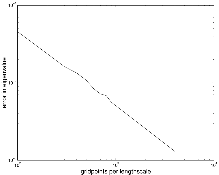
For our second convergence test we used the problem of an overtaking collision (illustrated in figure 6) between two right-propagating peakons. [2] gives a formula the phase-shifts for such a collision (i.e. the asymptotic difference in positions for the larger and smaller soliton with and without the collision). A plot of the error in the phaseshift against grid-size is given in figure 7.

We found that the performance of the method when solving for head-on peakon/anti-peakon interactions was quite poor. During the collision the two peakons approach each other and stick together once they are both within a grid width of each other. This appears to be an issue with representing the momentum using Lagrangian particles, as to achieve a method with the correct results for the collision, the particle momenta would need to go to infinity during the collision. However, we can also view this as a benefit of the method. The peakon/anti-peakon solution represents an instability in the equations; namely that a small perturbation of the solution can result in a peakon/anti-peakon pair being created. As our method does not support this solution at the moment of collision, this type of instability does not pollute our numerical results.

2D Flows

In this section we show a few results obtained using the VPM method to discretise EPDiff in two dimensions with Lagrangian

L=\frac{1}{2}\int|\boldsymbol{u}|^{2}+\alpha^{2}|\nabla\boldsymbol{u}|^{2}\diff{{}^{2}x},

for a constant lengthscale $\alpha$ so that the velocity $\boldsymbol{u}$ is obtained from the momentum $\boldsymbol{m}=\frac{\delta\boldsymbol{l}}{\delta\boldsymbol{u}}$ by inverting the modified Helmholtz operator

\boldsymbol{m}=(1-\alpha^{2}\Delta)\boldsymbol{u}.

In the first experiment the initial condition for the momentum had a 2-dimensional “top-hat” profile

\boldsymbol{m}=(m(x,y),0),\quad m=\left\{\begin{array}[]{c c}1&\mbox{ if }a<x<b,\quad c<y<d,\\ 0&\mbox{ otherwise.}\end{array},\right.

for constants $a,b,c,d$ , so that the velocity has continuous gradients and has compact support. Figure 8 shows the evolution of the velocity at subsequent times; it illustrates how EPDiff evolves to form singular filaments of momentum from smooth initial conditions.

Verification of conservation laws The next set of numerical results demonstrate the conservation of the right-action momenta given in section 6 and the connection with Kelvin’s circulation theorem.

Figure 10 shows the value of the momentum map for right action $\boldsymbol{P}_{\beta}\cdot J_{\beta}$ for a selection of particles from the flow in figure 8. All the particles have the same value because they all have the same initial momentum and $J$ is set to the identity initially. The figure shows that the numerical method preserves these conserved momenta up to round-off error. This follows from theorem 6.1 for the time continuous equations and the fact that conserved momentum maps are also conserved by variational integrators.

To verify the discrete circulation conservation discussed in section 7, we took an arbitrary loop containing some of the particles and advected the loop with the flow shown in figure 8, using

\boldsymbol{Q}^{n+1}(s)=\boldsymbol{Q}^{n}(s)+\sum_{k}\boldsymbol{u}_{k}\psi_{k}(\boldsymbol{Q}(s)),

where $s$ parameterises the loop. During the course of the flow this arbitrary circulation loop evolves, changing shape and length significantly. However, the circulation around the loop remains constant (up to numerical round off), as verified numerically in the following.

To write down the circulation integral, we choose an initial density

D_{k}=(M^{-1})_{kl}\sum_{\beta}\tilde{D}_{\beta}\psi_{k}(\boldsymbol{Q}_{\beta}),

where the values of $\tilde{D}$ do not matter much, as they are not coupled with the dynamics. Hence, we choose the values $\tilde{D}_{\beta}=1$ , $\beta=1,\ldots,N_{p}$ . To obtain the discretised loop integral

\sum_{\beta=1}^{N}\frac{\boldsymbol{P}_{\beta}}{\tilde{D}_{\beta}}\cdot\Delta\boldsymbol{x}_{\beta},

we need to calculate $\Delta\boldsymbol{x}_{\beta}$ as discussed in section 7. This is done by finding discrete line elements $\Delta\boldsymbol{x}_{\beta}^{0}$ for the initial loop and then calculating $\Delta\boldsymbol{x}$ for subsequent timesteps using

\Delta\boldsymbol{x}_{\beta}^{n}=J_{\beta}^{n}\cdot\Delta\boldsymbol{x}_{\beta}^{0}.

Summary of circulation loop figures

•

Figure 11 shows the evolution in time of this circulation loop, under the flow induced by the expanding waves in figure 8.
•

A plot showing initial and advected line elements is given in figure 12. This plot illustrates how the line elements evolve when a loop is stretched out by the flow. In the top and the bottom of the loop, where the stretching is greatest, one can see how the line elements extend to provide a numerical approximation to $d\boldsymbol{x}$ on the loop.
•

Finally a plot of the circulation integral is given in figure 13. This plot shows that the circulation round the loop is exactly preserved during the simulation (up to round-off error in the calculation of the discrete integral).

9 Summary and Outlook

In this paper we studied the Variational Particle-Mesh method applied to the EPDiff equation. We introduced a constrained variational principle for the method and gave discrete Euler-Poincaré formulae on the Eulerian grid resulting from the variational principle which show that the grid velocities and momenta satisfy the EPDiff equations in Eulerian form. Next we looked at left- and right-actions of velocity vector fields on the Lagrangian particles and obtained corresponding momentum maps. The left-action, when restricted to the finite space of velocity fields used in the method, gives rise to a momentum map which is the same formula as used for calculating the grid momentum from the particle variables. The right-action, which had to be interpreted in a wider space, can be interpreted as a discrete form of particle-relabelling since it corresponds to moving the particles and also changing the momenta in such a way so that the grid velocities remain constant. Finally we gave some interpretation of these transformations in terms of matrices which determine the local deformation of infinitesimal line elements, thereby allowing us to write down discrete loop integrals on advected loops. This led to a discrete circulation theorem.

Our next aim is to find an extension of this work which gives a discrete circulation theorem for fluid PDEs which involve mass density and other advected quantities as well as velocity. The general approach, following the continuous theory, will be to

•

specify the transformations corresponding to discrete relabelling,
•

determine the transformation of density and other advected quantities under this discrete relabeling group,
•

calculate the momentum densities obtained from these transformations.
•

show that the ratio of these momentum densities to the mass density is invariant.

Including advected quantities in this awy will allow introduction of potential energy and hence linear dispersion effects into the numerical description of the internal wave interactions using the VPM method.

Acknowledgements

We are grateful to our colleagues Joel Fine and Matthew Dixon at Imperial College London for their advice and consultation regarding this problem. We are also grateful to the ONR-NLIWI program for partial funding of this endeavor, and to Tony Liu for use of the SAR images of the South China Sea taken from the Space Shuttle. DDH is also grateful for partial support from the Office of Science, US Department of Energy.

References

[1] V. I. Arnold. Sur la géometrie differentielle des groupes de Lie de dimenson infinie et ses applications á la hydrodynamique des fluids parfaits. Ann. Inst. Fourier, (16):319–361, 1966.
[2] R. Camassa and D. D. Holm. An integrable shallow-water equation with peaked solitons. Physical Review Letters, 71(11):1661–1664, 1993.
[3] R. Camassa, D. D. Holm, and C. D. Levermore. Long-time effects of bottom topography in shallow water. Physica D, 98(2-4):258–286, Nov 1996.
[4] H. Cendra, J. E. Marsden, S. Pekarsky, and T. S. Ratiu. Variational principles for Lie-Poisson and Hamilton-Poincaré equations. Moskow Math. Journ., 3(3):833–867, 2003.
[5] C. J. Cotter. A general approach for producing Hamiltonian numerical schemes for fluid equations. http://arxiv.org/pdf/math.NA/0501468, 2005.
[6] C. Foias, D. D. Holm, and E. S. Titi. The Navier-Stokes-alpha model of fluid turbulence. Physica D, 2001.
[7] J. Frank, G. Gottwald, and S. Reich. A Hamiltonian particle-mesh method for the rotating shallow-water equations. In Lecture Notes in Computational Science and Engineering, volume 26, pages 131–142. Springer-Verlag, 2002.
[8] D. D. Holm and B. Kupershmidt. Poisson brackets and Clebsch representations for magnetohydrodynamics, multifluid plasmas, and elasticity. Physica D, 6:347–363, 1983.
[9] D. D. Holm, B. Kupfershmidt, and C. D. Levermore. Hamiltonian differencing of fluid dynamics. Adv. Appl. Math., pages 52–84, 1985.
[10] D. D. Holm and J. E. Marsden. Momentum maps and measure valued solutions (peakons, filaments, and sheets) of the Euler-Poincaré equations for the diffeomorphism group. In J.E. Marsden and T.S. Ratiu, editors, In The Breadth of Symplectic and Poisson Geometry, A Festshrift for Alan Weinstein, pages 203–235, Boston, MA., 2004. Birkhäuser Boston. http://arxiv.org/abs/nlin.CD/0312048.
[11] D. D. Holm, J. E. Marsden, and T. S. Ratiu. The Euler–Poincaré equations and semidirect products with applications to continuum theories. Adv. in Math., 137:1–81, 1998. http://arxiv.org/abs/chao-dyn/9801015.
[12] D. D. Holm, J. T. Rananather, A. Trouvé, and L. Younes. Soliton dynamics in computational anatomy. NeuroImage, 23:170–178, 2004. http://arxiv.org/abs/nlin.SI/0411014.
[13] A. Lew, J. E. Marsden, M. Ortiz, and M. West. An overview of variational integrators. In L.P. Franca, editor, Finite Element Methods: 1970s and Beyond. CIMNE, Barcelona, Spain, 2003.
[14] J. E. Marsden and A. Weinstein. Coadjoint orbits, vortices, and Clebsch variables for incompressible fluids. Physica D, 1983.
[15] M. I. Miller, A. Trouvé, and L. Younes. On the metrics and Euler-Lagrange equations of computational anatomy. Ann. Rev. Biomed. Engrg., 4:375–405, 2002.
[16] J. A. Yoder, S. G. Ankleson, R. T. Barber, P. Flament, and W. M. Balch. A line in the sea. Nature, (371):689–692, 1994.

Discrete momentum maps for lattice EPDiff

Abstract

1 Introduction

1.1 Transverse internal wave interactions

Plan of the paper

1.2 Theoretical development

Theorem 1.1 (Arnold (1966) [1]).

EPDiff

Variational Particle-Mesh (VPM) method

2 Particle-mesh calculus

A finite dimensional subspace of 𝔛⁡(Ω)\mathfrak{X}(\Omega)

Definition 2.1.

Remark 2.2.

Dynamics of a finite set of Lagrangian particles

Definition 2.3.

Definition 2.4 (The distribution DVPMD^{\VPM}).

Definition 2.5.

Remark 2.6.

Gradient and divergence

Definition 2.7.

Definition 2.8.

Discretised continuity equation

Lagrangian for semi-discrete EPDiff

Definition 2.9.

Remark 2.10.

3 Variational principle for discrete EPDiff

3.1 Constrained action principle for semi-discrete EPDiff

Definition 3.1 (Grid momentum).

Definition 3.2 (Constrained action).

Proposition 3.3.

Proof.

Remark 3.4.

Remark 3.5.

3.2 Legendre transform

Proposition 3.6.

Proof.

Proposition 3.7 (Hamilton’s canonical equations).

Proof.

3.3 Constructing a fully discrete method

4 The discrete Euler-Poincaré equation for VPM

Theorem 4.1 (Discrete Euler-Poincaré theorem).

Remark 4.2.

Proof.

Remark 4.3.

5 Left action momentum map

6 Right action momentum map

Right action of 𝔛⁡(Ω)\mathfrak{X}(\Omega) on {𝑸β​(t)}β=1np\{\boldsymbol{Q}_{\beta}(t)\}_{\beta=1}^{n_{p}}

Theorem 6.1.

Proof.

Corollary 6.2.

Proof.

Remark 6.3.

7 Kelvin’s circulation theorem for discrete EPDiff

Proposition 7.1.

Proof.

8 Numerical Results

2D Flows

9 Summary and Outlook

Acknowledgements

References

A finite dimensional subspace of $\mathfrak{X}(\Omega)$

Definition 2.4 (The distribution $D^{\VPM}$ ).

Right action of $\mathfrak{X}(\Omega)$ on $\{\boldsymbol{Q}_{\beta}(t)\}_{\beta=1}^{n_{p}}$