A VIRO THEOREM WITHOUT CONVEXITY HYPOTHESIS FOR TRIGONAL CURVES
Abstract
A cumbersome hypothesis for Viro patchworking of real algebraic curves is the convexity of the given subdivision. It is an open question in general to know whether the convexity is necessary. In the case of trigonal curves we interpret Viro method in terms of dessins d’enfants. Gluing the dessins d’enfants in a coherent way we prove that no convexity hypothesis is required to patchwork such curves.
1 Introduction
In†† Both authors are very grateful to the Max Planck Institute für Mathematik in Bonn for its financial support and excellent working conditions. the late†† 2000 Mathematics Subject Classification : 14P25 seventies†† Key words : topology of real algebraic curves, Viro method, dessin d’enfants, rational ruled surfaces O. Ya. Viro invented a powerful method to construct real algebraic hypersurfaces with prescribed topology in toric varieties. Since then it has become the main tool to prove the existence of certain topological types among families of real algebraic varieties.
Classification of the real schemes realized by nonsingular curves of degree in ([Vir84]), smoothing of curves with complicated singularities ([Vir89], [Shu99]), maximal curvature of plane algebraic curves ([LdM]), construction of counterexamples to the Ragsdale conjecture ([Ite93], [Ite01], [Haa95], [San] and [Bru06]) and construction of projective hypersurfaces with big Betti numbers ([Bih]) are examples of results using Viro method. It has also been used to prove maximality results. A real algebraic variety is said to be maximal (-variety) if the sum of the Betti numbers with coefficients of its real part is equal to the corresponding sum for its complexification . Viro method has been very useful to prove for instance the existence of projective -hypersurfaces of any degree in any dimension ([IV]) or existence of asymptotically maximal families of hypersurfaces in any projective toric variety ([Ber06]).
Roughly speaking , the Viro method (for curves) can be described as follows : start with some real algebraic curves whose Newton polygons are the -cells of a polygonal subdivision of a convex polygon . Then, under some assumptions on the ’s and on , the Viro Theorem asserts that there exists a real algebraic curve with Newton polygon obtained as a topological gluing of the curves . One of the hypothesis of Viro’s theorem is that the subdivision should be convex, i.e. there should exist a convex piecewise-linear affine function whose domains of linearity are exactly the Newton polygons of the curves . Notice that non-convex subdivisions do exist (see [CH80]), an example is depicted in Figure 2.
It is an open problem to know whether the convexity hypothesis is necessary or not. More precisely it is not known whether a curve patchworked from a non-convex subdivision is isotopic to a real algebraic curve with Newton polygon (see [dLW98] and [IS02]). I. Itenberg and E. Shustin proved in [IS02] that in the case of or of the geometrically ruled rational surfaces there always exists a real pseudoholomorphic curve isotopic to the patchworked one. Note that it is still unknown if there exists a real nonsingular pseudoholomorphic curve in which is not isotopic to a real nonsingular algebraic curve of the same degree.
If the convexity hypothesis in the Viro method turned out
to be necessary in general it could lead to such examples of
“non-algebraic pseudoholomorphic curves”.
On the other hand if the
convexity hypothesis could be removed it would simplify greatly the Viro
construction since it is often rather technical to check whether a given
subdivision is convex. Moreover this approach would give a deeper
insight or at least a new interpretation of the Viro method.
This work is a first step in the study of the need of the convexity
hypothesis.
Trigonal curves are those curves in whose Newton polygon is the triangle with vertices , and . In this article we prove that we can get rid of the convexity hypothesis for trigonal curves. Namely, any curve patchworked from is an algebraic trigonal curve in (with Newton polygon ). In fact we construct curves with prescribed positions with respect to the natural pencil of lines of . In the convex case, the pencil of lines has been studied by L. Lopez de Medrano in [LdM].
We want to construct a trigonal curve out of a trigonal patchwork. The strategy is the following. We first cut in several pieces which are the intersection of with some portions of the pencil of lines in . All these pieces are given by the subdivision of and will be algebraic. In [IS02], Itenberg and Shustin glue these pieces topologically in order to obtain a real pseudoholomorphic curve.
Since we deal with trigonal curve we are able to use a particular case of ”dessins d’enfants” which are called real rational graphs. This technic was introduced in real algebraic geometry independently by S. Yu. Orevkov in [Ore03] and by S. Natanzon, B. Shapiro and A. Vainshtein in [NSV02]. The position of a real trigonal curve with respect to the pencil in is encoded by three linearly dependent real polynomials (see [Ore03] or section 4). Real rational graphs give a necessary and sufficient condition for the existence of three linearly dependent real polynomials in one variable whose roots realize a given real arrangement. Via Riemann existence theorem they provide an existence criterion for a given trigonal curve.
In fact, we will use a slight generalization of these objects. To glue algebraically the pieces of our curve we indeed need to perform some surgery on dessins d’enfants enhanced with the data of the sign of some characteristic polynomials. These are what we call signed real rational graphs. Once glued together in a coherent way the signed real rational graphs obtained for each piece yield a dessin d’enfant which corresponds to a curve with the required topology.
Organization of this article
In section 2, we recall some facts about rational geometrically ruled surfaces. In section 3, we explain the patchwork construction and give a patchwork theorem for real algebraic trigonal curves without any convexity assumption (Theorem 3.4). We explain in section 4 how to encode the topology of a trigonal curve in a sign array. In section 5 we define an order on the polygons of a patchwork which is used in section 6 to extract a sign array from a trigonal patchwork. We state there our main result (Theorem 6.2) . The rest of the paper is devoted to the proof of this theorem. The main tool of this proof, signed real rational graphs, is defined in section 7. In section 8 we associate a signed real rational graph to each piece of the pencil of line given by the order on the polygons of a patchwork. We glue all these graph in section 9 and check in section 10 that the obtained signed real rational graph corresponds to a real algebraic trigonal curve which has the topology prescribed by the patchwork.
Notation
All polynomials in two variables are considered as polynomials in the variable whose coefficients are polynomials in the variable . By the discriminant of we mean the discriminant of with respect to the variable .
Suppose that a coordinate system of is fixed. The point (resp. ) is denoted by (resp.), and the points such that (resp. ) are called positive (resp. negative). The embedding of into given by induces an orientation of . Given two points and in , the segment is the connected component of oriented from to for this orientation.
When there is no ambiguity, the two words “curve” and “polynomial” are used to designate either a polynomial or the curve defined by this polynomial.
2 Rational geometrically ruled surfaces
The rational geometrically ruled surface, denoted by , is the surface obtained by taking four copies of with coordinates , , and , and by gluing them along with the identifications , and . Let us denote by (resp. and ) the algebraic curve in defined by the equation (resp. and ). The coordinate system is called standard. The projection : on defines a -bundle structure on which is extendable up to a -bundle structure on . The intersection numbers of and are respectively , and . The surface has a natural real structure induced by the complex conjugation in , and the real part of is a torus if is even and a Klein bottle if is odd. The restriction of on defines a pencil of lines denoted by .
The group is isomorphic to and is generated by the classes of and . Moreover, one has . An algebraic curve on is said to be of bidegree if it realizes the homology class in . Its equation in is
where is a homogeneous polynomial of degree . A curve of bidegree is called a trigonal curve on .
In the rational geometrically ruled surfaces, we study real curves up to isotopy with respect to . Two curves are said to be isotopic with respect to the fibration if there exists an isotopy of which transforms the first curve to the second one, and which maps each line of to another line of . In this paper, curves in a rational geometrically ruled surface are depicted up to isotopy with respect to .
Definition 2.1
An algebraic curve of bidegree in is said to be -nonsingular if is nonsingular and if for any fiber in , the set contains at least points.
3 Patchworking real algebraic trigonal curves
Here, we explain the patchworking method for curves. The general patchworking Theorem, which uses the convexity of the subdivision, can be found in [Vir84], [Vir89], [Vir], [Ris92] and [IS03]. Our patchwork Theorem, Theorem 3.4, does not require this convexity assumption, yet it works only for trigonal curves.
3.1 Chart of a real polynomial
This is the key notion of the Viro method. A chart of a real polynomial is a way to draw the curve defined by in in the union of 4 symmetric copies of its Newton polygon. The Newton polygon of a polynomial will be denoted by .
Given a convex polygon in with vertices in , one can define the so called moment map from to the interior of as follows
If , then is a diffeomorphism. For a pair , we denote by the symmetry of given by . For a convex polygon in , we define as .
Definition 3.1
Let be a real polynomial. The chart of , denoted by , is the closure of the set
It is clear that .
3.2 Gluing of charts
Let be a polynomial and be a face of .
Definition 3.2
The truncation of on is the polynomial .
The polynomial is totally nondegenerate if the truncation of to any face of is nonsingular in .
A patchwork is a way to glue together the charts of real algebraic curves.
Definition 3.3
Let be a convex polygon with vertices in . A patchwork with support is a pair such that
- •
is a subdivision of ,
- •
the are real algebraic curves,
- •
for any -cell of , there is one and only one curve whose Newton polygon is this polygon,
- •
for any edge of , the truncations on of two polynomials whose Newton polygon contains coincide.
If is the triangle with vertices , and and if the coefficient of of any curve is either or , we say that the patchwork is trigonal of degree .
As we deal with nonsingular curves, we will consider patchworks satisfying the following condition
- (1)
Each of the polynomials is totally nondegenerate.
Theorem 3.4
Let be a trigonal patchwork which satisfies hypothesis (1) above. Then there exists a real algebraic trigonal curve in whose chart is isotopic to .
Through all this paper, we will consider trigonal patchworks which satisfy one more condition. This condition is due to the fact that we construct curves which have a generic position with respect to the pencil of lines. This condition is a technical ingredient in the proof of Theorem 3.4. One can always perturb slightly the curves involved in a patchwork so that they satisfy this condition, hence it does not appear in the statement of Theorem 3.4.
- (2)
for any , the curves and have the maximal number of intersection points in among curves with fixed Newton polygon .
Remark : The last condition simply says that the curve has only ordinary tangency points with the vertical pencil of lines in and that none of these points lie on a toric divisor corresponding to a horizontal edge in the toric surface associated to .
We point out a consequence of condition (2) : suppose that and that (resp. ) with , then (resp. ).
4 The sign array of a real algebraic trigonal curve
4.1 Polynomials of degree 3 in one variable
Let us first consider a real polynomial of degree in one variable . It is well known that the following three numbers play an important role in the resolution of such an equation
The number is the discriminant of the polynomial . In particular one has
- •
if , then has three distinct real roots,
- •
if , then has one real root and two complex conjugated non-real roots,
- •
if and , then has a real double root and a simple real root and ,
- •
if and , then has a real double root and a simple real root and ,
- •
if and , then and has a real triple root.
Remark : under the change of variable , the numbers and are invariant and the number turns into its opposite.
4.2 Encoding the topology of a real algebraic trigonal curve
Let us now consider a -nonsingular real algebraic trigonal curve in . Let us choose a standard coordinate system on such that the fiber at infinity intersects in 3 distinct points (not necessarily real). The equation of in is
where is a polynomial of degree .
As in section 4.1, define the three following polynomial in one variable
The curve is -nonsingular so has only simple roots. Denote by the roots of . Denote also by the sign of with and the sign of for .
Definition 4.1
The sign array is called the sign array of the curve in the chosen standard coordinate system.
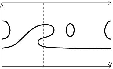
From the definition one can see that the sign array determines the position of a -nonsingular real algebraic trigonal curve in with respect to and conversely provided that a standard coordinate system has been chosen.
 |
 |
| a) | b) |
Example : Consider the trigonal curve on depicted in Figure 1a) and suppose that a standard coordinate system is chosen such that the vertical edges of the rectangle represent the fiber at infinity. Then the sign array of this trigonal curve is .
5 An order on the polygons of a subdivision
Let be the triangle with vertices , and and let be a subdivision of into convex integer polygons. We give an algorithm to put an order on the polygons of . In the Viro method, it will correspond to the order in which the polygons are scanned by the pencil of lines. Roughly speaking, the polygons will be scanned from the left to the right and only one polygon will be scanned at the same time except if it contains a horizontal edge. If two polygons have a horizontal edge in common, they will be scanned simultaneously by the pencil.
 |
In the procedure, is the current ordered subset of the 2-dimensional cells of , and is the set of remaining cells. The procedure starts with and . Perform the following operations until .
Step 1 : Suppose that and put
- •
,
- •
(i.e. is the left side of ),
- •
has an edge which is contained in
(i.e. elements of are the leftest polygons of ),
- •
, and has no horizontal edge containing
(i.e. we take pairs made of a polygon and a distinguished vertex of such that is the higher point of and is not on one of its horizontal edge),
- •
(i.e. we take the element of with the distinguished vertex of smaller ordinate).
Step 2 : Here we look for all the polygons which will be scanned at the same time by the pencil of lines.
Define by induction some polygons , where has been defined at step 1 : if shares a horizontal edge with a polygon , distinct from if , then put . Else, put and .
Step 3 : Put . If then also put .
Remark : in this algorithm, we “throw away” polygons corresponding to curves of degree 1 in and which do not have a horizontal edge of height 1.
Example : Applying this algorithm to the (non-convex) subdivision shown in Figure 2, one obtains
 |
Let be an element of and a polygon of .
Definition 5.1
The height of is defined as . The height of is the maximum of the heights of the polygons of .
Note that by construction, all the elements of have height at least 2.
6 The sign array associated to a trigonal patchwork
To a trigonal patchwork, we associate a sign array encoding the position that the curve we want to construct would have with respect to . This array is constructed studying where should be located the roots of the discriminant of the desired curve, and what should be the sign of at those points.
Let be a trigonal patchwork satisfying conditions (1) and (2) of section 3. Following what happens when the subdivision is convex (see [LdM]), the roots of will be obtained out of in exactly three different ways:
- •
any root in of the discriminant a curve of the patchwork gives rise to such a root ,
- •
suppose there is a horizontal edge of height 1 contained in a polygon of height at least 2 and in a polygon of height 1. The polygon corresponds in the patchwork to a curve of equation and the polygon corresponds to a curve of equation .
Then a root of of such that and have the same sign (see Figure 1b)) gives rise to two such roots .
- •
suppose there is a horizontal edge of height 2 contained in a polygon of height 3 and in a polygon of height 2. The polygon corresponds in the patchwork to a curve of equation and the polygon corresponds to a curve of equation .
Then a root of such that is positive (see Figure 4a)) gives rise to two such roots .
 |
 | |
| a) | b) |
First, we associate two lists of signs to each element of .
6.1 Lists of signs associated to an element of
Let be the element of and let be , and all the polynomials that occur in the polygons of . The polynomial is the coefficient of for some polygon of .
We define (resp. ) to be all the numbers in (resp. ) which verify one of the following conditions
- •
is a root of the discriminant of the curve corresponding to one of the polygons of ,
- •
two polygons of have a common horizontal edge of height 1, and is a root of such that and have the same sign (see Figure 1b)).
- •
two polygons of have a common horizontal edge of height 2, and is a root of such that is positive (see Figure 4).
6.1.1 is of height 3 and does not contain any polygon of height 2
That means that contains a polygon corresponding to a curve of degree and that no one of the comes from an edge of height 2. Denote by the sign of and perform the following substitutions in the lists and
- •
if is a root of the discriminant of the curve of degree 3, then replace by ,
- •
if is a root of , then replace by (see Figure 1b)).
Example : The two lists of signs associated to in the patchwork depicted in Figure 3 are and the empty list.
6.1.2 contains a polygon of height 2
That means that contains a polygon corresponding to a curve of degree . Denote by the sign of for small enough, and by the number of roots of counted with multiplicity which are strictly between and . Define and and perform the following substitutions in the lists and
Example : The two lists of signs associated to in the patchwork depicted in Figure 3 are the empty list and
6.2 The final sign array
So for each element of , we have defined two lists of signs and .
Define to be the coefficient of the monomial in the patchwork and put . Denote by the sign of the discriminant of .
Definition 6.1
The sign array associated to the patchwork is
Example : The sign array associated to the trigonal patchwork depicted in Figure 3 is
Theorem 6.2
Let be a trigonal patchwork of degree which satisfy the hypothesis (1) and (2) of section 3. Then there exists a -nonsingular real algebraic trigonal curve in realizing the sign array associated to .
Proof of Theorem 3.4: If the hypothesis (1) and (2) of section 3 are fulfilled, then Theorem 3.4 is a consequence of Theorem 6.2. Indeed, any -nonsingular real algebraic trigonal curve realizing the sign array associated to has a chart which is isotopic to the union of the charts used in the patchwork.
If only the hypothesis (1) is fulfilled, one can perturb slightly the coefficients of the curves used in the patchwork in order that the hypothesis (2) of section 3 is fulfilled. Then apply Theorem 6.2 to this patchwork. Perturbing in different ways the initial patchwork, one can construct -nonsingular real algebraic trigonal curve realizing different positions with respect to the pencil . However, all these curves have isotopic charts and this isotopy type is the one required by Theorem 3.4
7 Signed real rational graphs associated to trigonal curves and to curves of bidegree
7.1 Signed real rational graphs
Here we recall some fact about real rational graphs. We refer to [Bru06], [Bru], [Ore03] and [NSV02] for more details and proofs.
 |
 | |
| a) | b) |
Color and orient as depicted in Figure 5a).
Definition 7.1
Let be a graph on invariant under the action of the complex conjugation and a continuous map. Then the coloring and orientation of shown in Figure 5a) defines a coloring and an orientation of via .
The graph equipped with this coloring and this orientation is called a real rational graph if
- •
any vertex of has an even valence,
- •
for any connected component of , the map is a covering of of degree ,
- •
for any connected component of , the orientation induced by on is also induced by an orientation of .
The sum of the degrees for all connected component of of is called the degree of .
Since a real rational graph is invariant under the complex conjugation, we will draw in this article only one of the two halves of real rational graphs. This half will be drawn in a disk and the boundary of this disk will be .
Let be a real rational map of degree , and let be with the coloring and the orientation induced by those chosen on . Then is a real rational graph of degree .
Definition 7.2
One says that is the real rational graph associated to .
Example : the real rational graph associated to the real rational map is depicted in Figure 5b).
The next theorem shows that the converse is also true : one can construct real rational map out of a real rational graph.
Theorem 7.3
Let be a real rational graph of degree . Then there exists a real rational map of degree whose real rational graph is equivariantly isotopic to .
Such a real rational map is said to realize .
One of the steps in the proof of our main Theorem is the gluing of some real rational graphs. These gluings will not depend only on the real rational graphs, but also on some signs of polynomials which define it and on some coordinate system on . This motivates the notions of marked and signed real rational graphs.
Definition 7.4
A marked real rational graph is a real rational graph on where some coordinate system is fixed. In particular, the points and are prescribed on such a graph.
Let be a marked real rational graph and a real rational map which realizes . The marked graph is called a signed real rational graph if each connected component of is enhanced with a pair of signs.
As explained above, we will represent a real rational graph by a graph in a disk lying in . A marked real rational graph will be represented in a disk which is symmetric with respect to the -axis. If and are the two intersection points of and the circle bounding this disk with , then (resp. ) will be (resp. ) on the marked graph. The positive (resp. negative) points of will be drawn on the half plane (resp. ) and is called the positive (resp. negative) part of the graph.
In the rest of this paper, we will not draw the arrows on the real rational graphs.
Example : A signed real rational graph is depicted on figure 6b).
7.2 Signed real rational graph associated to a real algebraic trigonal curve in
Let be a real algebraic trigonal curve in . Then has the following equation in
where is a homogeneous polynomial of degree . To such a curve, we associate the real rational graph given by the map
where the polynomials and are those defined in section 4.2.
Definition 7.5
The graph is called the real rational graph associated to .
The preimages of by correspond to the roots of , the discriminant of . So if the curve is -nonsingular, according to section 4, one can recover the position of in with respect to up to the transformation only from .
 |
 | |
| a) | b) |
Example : the real rational graph associated to the trigonal curve in depicted on Figure 1a) is depicted in Figure 6a).
Conversely, suppose that using Theorem 7.3, we have constructed a real rational map out of a real rational graph . Then, is the real rational graph associated to the trigonal curve .
Up to rotation, this real rational graph does not depend on the coordinate system we choose on . If now we take into account the coordinate system, we obtain a marked real rational graph. Let us turn it into a signed real rational graph : the pair of signs on each connected component of is the pair formed by the sign of and the sign of on this component.
Definition 7.6
The graph is called the signed real rational graph associated to the polynomial .
Example : Suppose that we have fixed the coordinate system in such that the vertical edges of the rectangle in Figure 1a) are the fiber at infinity and the fiber in dotted line is the fiber at . Then is depicted in Figure 6b).
Note that the signed real rational graph associated to a trigonal curve in some coordinate system can be extracted from the knowledge of the real rational graph associated to this curve and the topology of the curve. For this reason, we won’t write explicitly the pairs of signs on signed real rational graph associated to trigonal curves in the rest of this paper.
Here we give a list of necessary and sufficient conditions for a signed real rational graph to be associated to some -nonsingular real algebraic trigonal curve. The proof can be found in [Ore03].
Proposition 7.7
Let be a signed real rational graph and let be a continuous map as in definition 7.1. Then there exists a -nonsingular real algebraic trigonal curve in such that is equivariantly isotopic to if and only if the following conditions are fulfilled
- •
is of degree ,
- •
any preimage of has an order which is divisible by ,
- •
any preimage of has an order which is divisible by ,
- •
any preimage of is of order ,
- •
any pair of sign labels a connected component of or ,
- •
any pair of sign labels a connected component of ,
- •
when passing through a preimage of of order , the pair of sign becomes .
7.3 Signed real rational graph associated to a real algebraic curve of bidegree (2,n) in
 |
 | |
| a) | b) |
Let be a real algebraic curve of bidegree in . So has the following equation in
where is a homogeneous polynomial of degree . The intersections of the curve with the exceptional divisor correspond to the roots of . To such a curve, we associate the real rational graph associated to the map
Definition 7.8
The graph is called the real rational graph associated to .
The real rational graph associated to the curve appears as a limit of the real rational graph associated to a real trigonal algebraic curve when its coefficient of tends to .
The preimages of by correspond to the roots of , the discriminant of .
Example : the real rational graph associated to the curve of bidegree in depicted in Figure 7a) is depicted in Figure 7b).
As in the case of trigonal curves, the real rational graph associated to does not depend on the coordinate system we choose on ,up to rotation. Taking into account the coordinate system chosen to write the equation of , we obtain a marked real rational graph. Let us turn it into a signed real rational graph : the pair of signs on each connected component of is the pair formed by the sign of and the sign of on this component.
Definition 7.9
The graph is called the signed real rational graph associated to the polynomial .
This definition of for a curve of bidegree is motivated by the fact that when we will glue together the curves of the patchwork in section 9, the topology coming from a curve of degree 2 will be encoded by the sign of (see Figure 4).
Note that the knowledge of the real rational graph and the topology of does not allow one to recover the sign real rational graph. Indeed, the sign of can be recovered neither from the real rational graph nor from the topology of the curve.
However, when the curve will be used in a patchwork, the sign of some other polynomials will allow us to recover the sign of .
8 Associating a signed real rational graph to any element of
 |
 |
 |
| a) | b) | c) |
 |
 |
 |
| a) | b) | c) |
Let be a trigonal patchwork of degree satisfying conditions (1) and (2) of section 3 and let be the -tuple constructed in section 5. We are going to associate a signed real rational graph to each . Dealing with charts of polynomials implies that a coordinate system is fixed. The signed real rational graphs will be constructed in this coordinate system.
8.1 is of height 2
Here we consider signed real rational graphs of curves of bidegree in . As mentioned in section 7.3, it cannot be extracted only from the knowledge of the real rational graphs of those curves and of their topology. However, when such a curve is used in a patchwork of a trigonal curve, one can recover the sign of out of this patchwork.
Indeed, if is a polygon of height in a trigonal patchwork, let be the leftest point of height of (i.e. ). Then, is an edge of the subdivision, and any curve of degree in the patchwork whose Newton polygon contains this edge prescribes the sign of for small values of : if the chart of one of these cubic intersect the edge (resp. ), then is negative for small positive (resp. negative) values of . This is because is of integer length and the coefficient of is .
For this reason, we will not write explicitly the pairs of signs on signed real rational graphs associated to a curve of bidegree in a trigonal patchwork.
8.1.1
That means that is the Newton polygon of a curve in the patchwork with a monomial and a non zero polynomial. Consider this curve as a curve of bidegree in , i.e. homogenize the curve in the following way :
where is a homogeneous polynomial of degree . This curve may have singular points on the fibers and .
Consider the signed real rational graph constructed in section 7.3. Then perturb this graph in such a way that all the preimages of are simple and perform all the operations depicted in Figure 10 on until the signed real rational graph has no ramification point on the preimage of . The first operation occurs in and the two last ones on .
The obtained signed real rational graph is .
 |
 |
 | ||
| a) | b) | c) |
Example : Let us detail how to find in the patchwork depicted in Figure 3. The corresponding curve is where , and are real numbers. Considering as a curve in , we have
Then is given by the real rational function
Then, according to the chart of , the real rational graph of is as depicted in Figure 8b). The chart of the curve corresponding to the polygon implies that is negative (resp. positive) for positive (resp. negative) values of . So is as depicted in Figure 8b).
8.1.2 with of height 2 and of height 1
Consider the signed real rational graph associated to the curve corresponding to as described in section 8.1.1. This curve is the union of a curve of degree 1 and the curve . So all the roots of its discriminant are double and correspond to the intersection points of and . The curve corresponding to tells us how to smooth these double points. More precisely, write and and suppose that is a root of in . Then if and have the same sign (resp. opposite signs), then perturb the corresponding double root of the discriminant on into 2 distinct real roots (resp. non-real roots) as depicted in Figure 11a) (resp. 11b)).
 |
 | |
| a) | b) |
The graph is the obtained signed rational graph.
Remark : The graph is , where is the perturbation of prescribed by .
8.2 is of height 3
8.2.1
The curve in the patchwork corresponding to is a real algebraic trigonal curve, nonsingular in and we define to be .
8.2.2 with of height 3 and of height 1
Consider the signed real rational graph associated to the curve corresponding to as described in section 8.2.1. This curve is the union of a curve (nonsingular in ) of degree 2 and the curve and all the double roots of its discriminant correspond the intersection points of and . The curve corresponding to tells us how to smooth these double points. More precisely, write and and suppose that is a root of in . Then if and have the same signs (resp. opposite signs), then perturb the corresponding double root of the discriminant of the curve into 2 distinct real roots (resp. non-real roots) as in section 8.1.2.
The graph is the obtained signed rational graph.
Remark : The graph is , where is the perturbation of prescribed by . In particular, is always the signed real rational graph associated to a trigonal curve.
8.2.3 with of height 3 and of height 2
 |
 |
| a) | b) |
 |
First, consider as explained in section 8.1.1. We will obtain performing some modifications on .
Let be a root of in . Choose a real rational function realizing and such that has no ramification point on the connected component of containing .
Then replace by
The graph is the obtained signed rational graph.
8.2.4 with of height 3, of height 2 and of height 1
First, consider as explained in section 8.1.1. Then, perturb all the roots of in as explained in section 8.2.3 and perturb all the double roots of the discriminant as explained in section 8.1.2.
The graph is the obtained signed rational graph.
9 Gluing of signed real rational graphs
Let be a trigonal patchwork of degree satisfying conditions (1) and (2) of section 3 and let be the -tuple constructed in section 5. In this section, we describe how to glue all the signed real rational graphs in order to obtain a new signed real rational graph corresponding to a nonsingular real trigonal algebraic curve in .
For , we describe how to glue the signed real rational graph corresponding to to the one corresponding to .
Example : To illustrate this procedure, we have depicted in Figure 18 all the steps in the gluing process corresponding to the patchwork depicted in Figure 3.
9.1 and are of height 3 and contain no polygon of height 2
That means that both and contain a polygon which have the edge with in common.
As noticed in section 8, and correspond to two real algebraic trigonal curves, respectively and . In particular, the two real rational graphs are given by two real rational maps
The second form of and are required to be irreducible and we point out that can be different from .
The method here is the following : identify in and in . We obtain something which is not any more a signed real rational graph, but some kind of signed singular real rational graph. This is a graph on two copies of which are identified in one point, for one of them and for the other one. Smoothing equivariantly this point we will obtain a smooth signed real rational graph on .
9.1.1 or
From condition we get that and . Moreover, one can perturb slightly the coefficients corresponding to the integer vertices of such that . This implies that .
 |
 | |
| a) | b) |
Then, as the truncation on of and coincide, the pair of signs on the positive (resp. negative) part of near and near also coincide. Suppose that is in . Then, smooth the singular real rational graph as depicted in Figure 14a) or b), depending on the situation. The case when is in or can be treated analogously.
 |
|
| a) |
9.1.2 or
We treat the case , the case being symmetric.
In this case, a simple computation shows that is a root of order of and that is a root of order of , where and are some natural numbers. Perturbing if necessary the coefficient of and , one can suppose . Moreover, as the truncation on of and coincide, the pair of signs on the positive (resp. negative) part of near and near also coincide. Then, smooth the singular real rational graph as depicted in Figure 15 or symmetrically with respect to the axis , depending on the situation.
9.1.3
 |
 | |
| a) | b) |
In this case, a simple computation shows that is a root of order of and that is a root of order of , where and are some natural numbers. Perturbing if necessary the coefficient of and , one can assume that . If is the pair of signs on the positive part of (resp. ) near (resp. ), then the pair of signs on the negative part of (resp. ) near (resp. ) is (resp. ). Moreover, as the truncation on of and coincide, the sign of the discriminant on the positive (resp. negative) part of near and near also coincide.
Then, depending on the situation, smooth the singular real rational graph using the appropriate perturbation among those depicted in Figure 16 and their symmetric with respect to the axis .
9.2 or contains a polygon of height 2
Let be the point of the polygons of of ordinate 2 with maximal abscissa. Let be the unique edge of the form with which is a common edge of a polygon of and of a polygon of . The line supported by intersects the line in the point (see figure 17).
We suppose that . The case can be recovered by symmetry.
Let (resp. ) be the curve of the patchwork corresponding to (resp. ) and (resp. ) be the real rational map constructed out of (resp. ) as explained in section 7. Here again, the polynomials and (resp. and ) have no common factor.
According to section 8, the graph (resp. ) is either (resp. ) or a perturbation of this signed real rational graph in some points distinct from and . So, the gluing of and is determined by the neighborhood of in and in .
 |
 |
| a) | b) |
A simple calculation shows that
- •
if is an integer, then (resp. ) is a root of order of (resp. ),
- •
if is not an integer, then (resp. ) is a root of order of (resp. ),
where denote the integer part of the real .
It follows from the construction of and and from condition (1) of section 3 that the pair of signs on the positive (resp. negative) part of near and near also coincide.
Let be the connected component of which contains . Then cut from , cut from and glue it in the only possible way, as it is depicted on Figure 17b) in a particular case.
 |
 |
 | ||
| a) | b) | c) |
10 Proof of Theorem 6.2
Let be a trigonal patchwork of degree satisfying conditions (1) and (2) of section 3. In this section, we show that the signed real rational graph constructed in section 9 out of corresponds to a -nonsingular real trigonal algebraic curve in which realizes the sign array of the corresponding patchwork.
First, we check that is the signed real rational graph of a -nonsingular real trigonal algebraic curve in . The only non-trivial part is to prove that the degree of is . In order to compute it, we count the number of preimages of 1. So we first have to count how many preimages of 1 each element of brings to . According to section 9, this is equivalent to count how many preimages of are lying on for all element of .
First, we count the number of roots in of the discriminant of a curve. Given a convex polygon , the quantity is the number of integer points in the interior of and denotes the number of integer points of the boundary of which have neither a maximal nor a minimal ordinate.
Lemma 10.1
Let be a totally nondegenerate curve with Newton polygon . Then, the discriminant of has roots in counted with multiplicity.
Proof : Let us consider the closure of in and the rational map given by . It is well known that the genus of the normalization of is . So, applying the Riemann Hurwitz formula to the restriction of to , we have
where , is the number of roots (counted with multiplicity) in of the discriminant of and is the sum of the tangency order of local branches of along and . As is totally nondegenerate, we have , so
The Lemma is proved.
Corollary 10.2
The real rational graph constructed out of a trigonal patchwork of degree is of degree .
Proof : It is clear from the construction and the hypothesis on the trigonal patchwork that the degree of is equal to the sum of the numbers of preimages of in for all in . From section 8 and Lemma 10.1, we know that this number is equal to which is equal to .
Proposition 10.3
The signed real rational graph is realizable by a -nonsingular real algebraic trigonal curve in .
Proof : The degree of is given by Corollary 10.2 and all the other conditions of Proposition 7.7 are satisfied by construction.
Choose a standard coordinate system on such that the point on corresponds to the fiber at infinity and let be the sign array of the curve in this coordinate system.
Proposition 10.4
Proof : Let (resp. ) be the sign array (resp. associated to the patchwork). First note that a direct consequence of sections 6, 8 and 9 is that , i.e. both curves have the same number of tangency points with the pencil of vertical lines. Hence, to prove Theorem 6.2, we have just have to prove that for any .
It is clear from sections 6, 8 and 9 that both and come from the same real for some . Choose a real rational map which realize .
If contains no polygon with a horizontal edge of height , then corresponds to a root of the discriminant of a curve of whose Newton polygon is in . Hence, which is the sign of , is the second element of the pair of signs which labels near . But according to section 6, this is also .
If contains a polygon with a horizontal edge of height , denote by the polynomial corresponding to this edge. Let be the number of roots of counted with multiplicity which are strictly between and and let be the sign of for small enough with the same sign as . There are two possibilities, each of them can checked directly from the construction of .
- •
If is not a root of , then .
- •
If is a root of , then gives rise to two elements of both sign arrays, say , , and . We have and .
So in any case, we have .
11 Remark on an equivariant version Theorem 3.4
We were guided in this work by the following observation : the position of the real part of a nonsingular real algebraic curve in with respect to the pencil of lines is totally encoded by the sign array realized by some collection of polynomials in one variable, namely the leading coefficients of some signed subresultant sequences (see [BPR03] or [Hon] for example). It seems to us that this observation could lead to interesting results in real algebraic geometry, especially in the study of the need of convexity in patchworking.
In the case of trigonal curves, the polynomials whose sign array encode the topology of the real part of the curve are exactly, with notation of section 4, the polynomials , and . Moreover, such three polynomials with a prescribed sign array can be constructed using signed real rational graphs.
On the other hand, real rational graphs carry much more informations than the knowledge of the topology of the real part of real algebraic curves. Indeed, one can extract the position with respect to the pencil of lines of the complexification of any real trigonal curve out of its associated real rational graph. Hence, one can consider not only isotopies of curves in the real part of the surface but also equivariant isotopies of curves in . That means that it is possible to state an equivariant version of Theorem 3.4 and Theorem 6.2.
Proving such an equivariant statement would carry us quite far away from our original framework. So we only give the main ingredients needed in its formulation and in its proof.
- Step 1.
-
In the patchwork construction, one can use complexification of lattice polygons and complex equivariant charts of real polynomials as defined in [IS02], [IS03] and [Vir]. Then, the patchwork procedure gives a piecewise smooth surface, invariant under the action of the complex conjugation, in the complexification of the triangle with vertices , and .
- Step 2.
-
One can use the braid monodromy factorization (see [KT00] or [KK03] for example) to encode the position of a complex algebraic curve in with respect to the pencil of lines. An equivariant version of this encoding, based on previous papers by Orevkov (see [Ore99] for example), should be used to deal with real algebraic curves.
- Step 3.
-
As we associated a sign array to a trigonal patchwork (in section 6), one can associate in a similar way an equivariant braid monodromy factorization to an equivariant trigonal patchwork (defined in Step 1).
- Step 4.
References
- [Ber06] B. Bertrand. Asymptotically maximal families of hypersurfaces in toric varieties. Geom. Dedicata., 118(1):49–70, 2006.
- [Bih] F. Bihan. Asymptotiques de nombres de Betti d’hypersurfaces projectives réelles. Preprint arXiv: math.AG/0312259, (French).
- [BPR03] S. Basu, R. Pollack, and M. F. Roy. Algorithms in real algebraic geometry, volume 10 of Algorithms and Computation in Mathematics. Springer-Verlag, Berlin, 2003.
- [Bru] E. Brugallé. Symmetric plane curves of degree 7 : pseudo-holomorphic and algebraic classifications. arXiv : math.GT/0404030.
- [Bru06] E. Brugallé. Real plane algebraic curves with asymptotically maximal number of even ovals. Duke Math. J., 131(3):575–587, 2006.
- [CH80] R. Connelly and D. W. Henderson. A convex 3-complex not simplicially isomorphic to a strictly convex complex. Proc. Camb. Phil. Soc., 88(2):299–306, 1980.
- [dLW98] J. A. de Loera and F. J. Wickiln. On the need of convexity in patchworking. Adv. in Appl. Math., 20:188–219, 1998.
- [Haa95] B. Haas. Les multilucarnes: nouveaux contre-exemples à la conjecture de Ragsdale. C. R. Acad. Sci. Paris Sér. I Math., 320(12):1507–1512, 1995. (French).
- [Hon] H. Hong. Subresultants in root. submitted, available at http://www4.ncsu.edu/˜hong/papers.html.
- [IS02] I. Itenberg and E. Shustin. Combinatorial patchworking of real pseudo-holomorphic curves. Turkish J. Math., 26(1):27–51, 2002.
- [IS03] I. Itenberg and E. Shustin. Viro theorem and topology of real and complex combinatorial hypersurfaces. Israel J. Math., 133:189–238, 2003.
- [Ite93] I. Itenberg. Contre-exemples à la conjecture de Ragsdale. C. R. Acad. Sci. Paris Sér. I Math., 317(3):277–282, 1993. (French).
- [Ite01] I. Itenberg. On the number of even ovals of a nonsingular curve of even degree in . In Topology, ergodic theory, real algebraic geometry, volume 202 of Amer. Math. Soc. Transl. Ser. 2, pages 121–129. Amer. Math. Soc., Providence, RI, 2001.
- [IV] I. Itenberg and O. Ya. Viro. Maximal real algebraic hypersurfaces of projective spaces. in preparation.
- [KK03] V. S. Kulikov and V. M. Kharlamov. On braid monodromy factorizations. Izv. Ross. Akad. Nauk Ser. Mat., 67(3):79–118, 2003.
- [KT00] V. S. Kulikov and M. Taĭkher. Braid monodromy factorizations and diffeomorphism types. Izv. Ross. Akad. Nauk Ser. Mat., 64(2):89–120, 2000.
- [LdM] L. Lopez de Medrano. Courbure totale des variétés algébriques réelles projectives. Thèse doctorale, 2006, (French).
- [NSV02] S. Natanzon, B. Shapiro, and A. Vainshtein. Topological classification of generic real rational functions. J. Knot Theory Ramifications, 11(7):1063–1075, 2002.
- [Ore99] S. Yu. Orevkov. Link theory and oval arrangements of real algebraic curves. Topology, 38(4):779–810, 1999.
- [Ore03] S. Yu. Orevkov. Riemann existence theorem and construction of real algebraic curves. Annales de la Faculté des Sciences de Toulouse, 12(4):517–531, 2003.
- [Ris92] J. J. Risler. Construction d’hypersurfaces réelles (d’après Viro). Séminaire Bourbaki, 763, 1992. (French).
- [San] F. Santos. Unpublished.
- [Shu99] E. Shustin. Lower deformations of isolated hypersurface singularities. Algebra i Analiz, 11(5):221–249, 1999.
- [Vir] O. Ya. Viro. Patchworking real algebraic varieties. http://www.math.uu.se/oleg.
- [Vir84] O. Ya. Viro. Gluing of plane real algebraic curves and constructions of curves of degrees and . In Topology (Leningrad, 1982), volume 1060 of Lecture Notes in Math., pages 187–200. Springer, Berlin, 1984.
- [Vir89] O. Ya. Viro. Real plane algebraic curves: constructions with controlled topology. Leningrad Math. J., 1(5):1059–1134, 1989.
| Benoît Bertrand | Erwan Brugallé | |
| Section de mathématiques | Max Planck Institute für Mathematik | |
| Université de Genève | Vivatsgasse, 7 | |
| case postale 64, | D-53111 Bonn | |
| 2-4 rue du Lièvre, | Deutschland | |
| Genève | ||
| Suisse | ||
| E-mail : benoit.bertrand@math.unige.ch | E-mail : brugalle@mpim-bonn.mpg.de |