Conformally invariant scaling limits
an overview and a collection of problems

To motivate SLE, we now discuss percolation. More specifically, we define one particular model of percolation in two dimensions. Fix a number $p\in[0,1]$. Let $\omega$ be a random subset of the set of vertices in the triangular grid $\mathrm{TG}$, where for vertices $v\in V(\mathrm{TG})$ the events $v\in\omega$ are independent and have probability $p$. In percolation theory one studies the connected components (a.k.a. clusters) of the random subgraph of $\mathrm{TG}$ whose vertex set is $\omega$ and whose edges are the edges in $\mathrm{TG}$ connecting two elements of $\omega$. Equivalently, one may study the connected components of the set of white hexagons in Figure 1, where each hexagon in the hexagonal grid dual to $\mathrm{TG}$ represents a vertex of $\mathrm{TG}$ and hexagons corresponding to vertices in $\omega$ are colored white. The reasons for considering this dual representation are that the figures come out nicer and that it makes some important definitions more concise.

The above percolation model is site (or vertex) percolation on the triangular grid. Likewise, there is a bond (or edge) model, where one considers a random subgraph of a grid whose vertex set is the set of all vertices of the grid, but where each edge of the grid is in the percolation subgraph with probability $p$, independently. Additionally, there are various percolation models which are not based on a lattice. Some of these will be discussed in later sections.

There is an important value $p_{c}$ of the parameter $p$, which is the threshold for the existence of an unbounded cluster and is called the critical value of $p$. The actual value of $p_{c}$ varies depending on the particular percolation model. For site percolation on the triangular grid, as well as for bond percolation on the square grid, we have $p_{c}=1/2$. This is a theorem of Kesten [43], based on earlier work by Harris [33], Russo [78] and Seymour and Welsh [84]. The underlying reason for this nice value of $p_{c}$ is a duality which these two models have, though the precise form of the duality they exhibit is different. For bond percolation on the triangular grid $p_{c}=2\,\sin(\pi/18)$ [98], while for site percolation on the square grid there is not even a prediction for the value of $p_{c}$, though rigorous and experimental estimates exist. As $p$ increases beyond $p_{c}$, the large scale behavior of percolation undergoes a rapid change. This is perhaps the mathematically simplest model of a phase transition. From now on, we will focus our attention on critical percolation, that is, percolation with $p=p_{c}$, which is in many ways the most interesting value of $p$.

We now define and discuss the percolation interface curve indicated in Figure 2. Consider a bounded domain $D$ in the plane ${\mathbb{R}}^{2}={\mathbb{C}}$ whose boundary is a simple closed curve. Let $\partial_{+}\subset\partial D$ be a proper arc on the boundary of $D$. Given $\epsilon>0$ we may consider the collection of hexagons in a hexagonal grid of mesh $\epsilon$ which intersect $\overline{D}$. Each of these hexagons which meets $\partial_{+}$ we color white, each of the hexagons which meet $\partial D$ but not $\partial_{+}$ we color black, and each of the hexagons contained in $D$ we color white or black with probability $1/2$, independently. In addition to white clusters (connected components of white hexagons) sometimes, black clusters are also considered. Percolation theory is the study of connected components of random sets, such as these clusters.

For simplicity, we assume that $\partial D$ is sufficiently smooth and $\epsilon$ is sufficiently small so that the union of hexagons intersecting $\partial D$ but not $\partial_{+}$ is connected. There is a unique (random) path $\beta$, which is the common boundary of the white cluster meeting $\partial_{+}$ and the black cluster meeting $\partial D$.

The law $\mu_{D,\partial_{+},\epsilon}$ of $\beta$ is a probability measure on the space of closed subsets of $\overline{D}$ with the Hausdorff metric. Smirnov [87] proved that as $\epsilon\searrow 0$ the measure $\mu_{D,\partial_{+},\epsilon}$ converges weakly to a measure $\mu_{D,\partial_{+}}$, and that $\mu$ is conformally invariant, in the following sense. If $f:\overline{D}\to\overline{D^{\prime}}\subset{\mathbb{R}}^{2}$ is a homeomorphism that is analytic in $D$, then the push forward of $\mu_{D,\partial_{+}}$ under $f$ is $\mu_{f(D),f(\partial_{+})}$. In other words, if $\epsilon$ is small, then $f(\beta)$ is a good approximation for the corresponding path defined using a hexagonal grid of mesh $\epsilon$ in $f(D)=D^{\prime}$. This type of conformal invariance was believed to hold for many “critical” random systems in two dimensions. However, the only previous result establishing conformal invariance for a random scaling limit is Lévy’s theorem [64] stating that for two-dimensional Brownian motion, the scaling limit of simple random walk on ${\mathbb{Z}}^{2}$, is conformally invariant up to a time-change.

Smirnov’s proof is very beautiful, and the result is important, but describing the proof will throw us too far off course (since for this paper percolation is just an example model, not the primary topic). The interested reader is encouraged to consult [12, 30, 70, 45] for background in percolation and highlights of percolation theory. An elegant simplification of parts of Smirnov’s proof has been discovered by Vincent Beffara [11]. A more detailed version of other parts of Smirnov’s argument appears in [19].

Though this was not the original inspiration, we will now use Smirnov’s result to motivate the definition of SLE. By conformal invariance, we may venture to understand $\beta$ in the domain of our choice. The simplest situation turns out to be when $D=\mathbb{H}$ is the upper half plane and $\partial_{+}$ is the positive real ray ${\mathbb{R}}_{+}$, as in Figure 3. (Though this domain $D$ is unbounded, that does not cause any problems.) We may consider the discrete path $\beta$ as a simple path $\beta:[0,T)\to\overline{\mathbb{H}}$ starting near $0$ and satisfying $\lim_{t\to T}|\beta(t)|=\infty$ (where $T$ is finite or infinite).

We would like to learn about $\beta$ by understanding the one-parameter family of conformal maps $g_{t}$ mapping $\mathbb{H}\setminus\beta([0,t])$ onto $\mathbb{H}$. To facilitate this, we must first recall a few basic facts and discuss Loewner’s theorem. At this point, assume only that $\beta$ is a simple path in $\overline{\mathbb{H}}$ with $\beta(0)\in{\mathbb{R}}$ and $\beta(t)\notin{\mathbb{R}}$ for $t>0$. The existence of the conformal maps $g_{t}:\mathbb{H}\setminus\beta([0,t])\to\mathbb{H}$ is guaranteed by Riemann’s mapping theorem. However, $g_{t}$ is not unique. In order to choose a specific $g_{t}$ for every $t$, we first require that $g_{t}(\infty)=\infty$. Schwarz reflection in the real axis implies that $g_{t}$ is analytic in a neighborhood of $\infty$, and therefore admits a power series representation in $1/z$,

valid for all $z$ sufficiently large. Since $g_{t}$ maps the real line near $\infty$ into the real line, it follows that $a_{j}\in{\mathbb{R}}$ for all $j$, and because $g_{t}:\mathbb{H}\setminus\beta([0,t])\to\mathbb{H}$, we find that $a_{1}>0$. We now pick a specific $g_{t}$ by imposing the so-called hydrodynamic normalization at $\infty$, namely $a_{1}=1$ and $a_{0}=0$. This can clearly be achieved by post-composing with a map of the form $z\mapsto a\,z+b$, $a>0$, $b\in{\mathbb{R}}$.

The coefficients $a_{j}$ of the series expansion of $g_{t}$ are now functions of $t$. It is not hard to verify that $a_{-1}(t)$ is a continuous, strictly increasing function of $t$. Clearly, $g_{0}(z)=z$ and hence $a_{-1}(0)=0$. We may therefore reparametrize $\beta$ so as to have $a_{-1}(t)=2\,t$ for all $t>0$. This is called the half-plane capacity parametrization of $\beta$. With this parametrization, a variant of Loewner’s theorem [65] states that the maps $g_{t}$ satisfy the differential equation

where $W(t):=g_{t}\bigl(\beta(t)\bigr)$ is called the Loewner driving term. A few comments are in order.

1. 1.

   Although $g_{t}$ is defined in $\mathbb{H}\setminus\beta([0,t])$, it does extend continuously to $\beta(t)$, and therefore $W(t)$ is well defined.

2. 2.

   If $z=\beta(s)$ for some $s$, then (1) makes sense only as long as $t<s$. That is to be expected. The domain of definition of $g_{t}$ is shrinking as $t$ increases. A point $z$ falls out of the domain of $g_{t}$ at the first time $\tau=\tau_{z}$ such that $\liminf_{t\nearrow\tau}g_{t}(z)-W(t)=0$.

3. 3.

   The main point here is that information about the path $\beta$ is encoded in $W(t)$, which is a path in ${\mathbb{R}}$.

4. 4.

   The proof of (1) is not too hard. In [53, Theorem 2.6] a proof (of a generalization) may be found.

We now return to the situation where $\beta$ is the percolation interface chosen according to $\mu_{\mathbb{H},{\mathbb{R}}_{+},\epsilon}$, parametrized by half-plane capacity. It is easy to see that in this case $T=\infty$. Fix some $s>0$. Suppose that we examine the colors of only those hexagons that are necessary to determine $\beta([0,s])$. This can be done by sequentially testing the hexagons adjacent to $\beta$ starting from $\beta(0)$ as follows. Each time the already determined arc of $\beta$ meets a hexagon whose color has not yet been examined, we test the color (which permits us to extend the determined initial arc of $\beta$ by at least one segment), until $\beta([0,s])$ has been determined. See Figure 4.

Now comes the main point. Let $D_{s}$ be the unbounded component of the collection of hexagons of undetermined color in $\mathbb{H}$, and let $\partial_{+}^{s}$ be the subset of $\partial D_{s}$ lying on the boundary of hexagons of determined color white. Then the distribution of the continuation $\beta([s,\infty))$ of the interface given $\beta([0,s])$ is $\mu_{D_{s},\partial_{+}^{s},\epsilon}$. By Smirnov’s theorem, if $G:D_{s}\to\mathbb{H}$ is the conformal map satisfying the hydrodynamic normalization, then the image under $G$ of $\mu_{D_{s},\partial_{+}^{s},\epsilon}$ is close to $\mu_{\mathbb{H},G(\partial_{+}^{s}),\epsilon}$. (Actually, to justify this, one needs a slightly stronger “uniform” version of Smirnov’s theorem. But here we want to convey the main ideas, and do not bother about being entirely precise.) Now, since $D_{s}$ approximates $\mathbb{H}\setminus\beta([0,s])$, it follows that $G$ is very close to $g_{s}$ and $G(\partial_{+}^{s})$ is close to $[W(s),\infty)=[g_{s}(\beta(s)),\infty)$. Therefore, in the limit as $\epsilon\searrow 0$, we have for $\beta$ sampled according to $\mu_{\mathbb{H},{\mathbb{R}}_{+}}$ that given $\beta([0,s])$ the distribution of $g_{s}\circ\beta([s,\infty))$ (which is the conformal image of the continuation of the path) is $\mu_{\mathbb{H},{\mathbb{R}}_{+}}$ translated by $W(s)$.

The Loewner driving term of the path $t\mapsto g_{s}\circ\beta(s+t)$ is $W(s+t)$, because $g_{s+t}\circ g_{s}^{-1}$ maps $\mathbb{H}\setminus g_{s}\bigl(\beta([s,s+t])\bigr)$ onto $\mathbb{H}$. The conclusion of the previous paragraph therefore implies that given $(W(t):t\in[0,s])$ the distribution of the continuation of $W$ is identical to the original distribution of $W$ translated to start at $W(s)$. This is a very strong property. Indeed, for every $n\in{\mathbb{N}}$ and $t>0$ we may write $W(t)=\sum_{j=1}^{n}\bigl(W(j\,t/n)-W((j-1)t/n)\bigr)$, which by the above is a sum of $n$ independent identically distributed random variables. If we assume that the variance of $W(t)$ is finite, then it is also the sum of the variances of the summands. By the central limit theorem, $W(t)$ is therefore a Gaussian random variable. By symmetry, $W(t)$ has the same distribution as $-W(t)$, and so $W(t)$ is a centered Gaussian. It now easily follows that there is some constant $\kappa\geq 0$ such that $W(t)$ has the same distribution as $B(\kappa\,t)$, where $B$ is one-dimensional Brownian motion starting at $B(0)=0$. Using results from the theory of stochastic processes (e.g., the characterization of continuous martingales as time-changed Brownian motion), the same conclusion can be reached while replacing the assumption that $W(t)$ has finite variance with the continuity of $W(t)$ in $t$.

We have just seen that Smirnov’s theorem implies that the Loewner driving term of a sample from $\mu_{\mathbb{H},{\mathbb{R}}_{+}}$ is $B(\kappa\,t)$ for some $\kappa\geq 0$. This should serve as adequate motivation for the following definition from [79].

Of course, $\mathrm{SLE}_{\kappa}$ is a random one-parameter family of maps; the randomness is entirely due to the Brownian motion.

It has been proven [76, 59] that with probability $1$ there is a (unique) random continuous path $\gamma(t)$ such that for each $t\geq 0$ the domain of definition of $g_{t}$ is the unbounded component of $\mathbb{H}\setminus\gamma([0,t])$. The path is given by $\gamma(t)=g_{t}^{-1}(W(t))$, but proving that $g_{t}^{-1}(W(t))$ is well defined is not easy. It is also known [76] that a.s. $\gamma(t)$ is a simple path if and only if $\kappa\leq 4$ and is space-filling if and only if $\kappa\geq 8$. Sometimes the path $\gamma$ itself is called $\mathrm{SLE}_{\kappa}$. This is not too inconsistent, because $g_{t}$ can be reconstructed from $\gamma([0,t])$ and vice versa.

If $D$ is a simply connected domain in the plane and $a,b\in\partial D$ are two distinct points (or rather prime ends), then chordal SLE from $a$ to $b$ in $D$ is defined as the image of $\gamma$ under a conformal map from $\mathbb{H}$ to $D$ taking $0$ to $a$ and $\infty$ to $b$. Though the map is not unique, the choice of the map does not effect the law of the SLE in $D$. This follows from the easily verified fact that up to a rescaling of time, the law of the SLE path is invariant under scaling by a positive real constant, as is the case for Brownian motion.

The reason for calling the SLE “chordal” is that it connects two boundary points of a domain $D$. There is another version of SLE, which connects a boundary point to an interior point, called radial SLE. Actually, there are a few other variations, but they all have similar definitions and analogous properties.

In this subsection we list some works and discoveries related to SLE and random scaling limits in two dimensions. The following account is not comprehensive. Some of the topics not covered here are discussed in Wendelin Werner’s [97] contribution to this ICM proceedings. We start by very briefly discussing the historical background.

In the survey paper [49], Langlands, Pouliot and Saint-Aubin present a collection of intriguing predictions from statistical physics. They have discussed these predictions and some simulation data with Aizenman, which prompted him to conjecture that the critical percolation crossing probabilities are asymptotically conformally invariant (see [49]). This means that the probability $Q_{\epsilon}(D,\partial_{1},\partial_{2})$ that there exists a critical percolation cluster in a domain $D\subset{\mathbb{C}}$ connecting two boundary arcs $\partial_{1}$ and $\partial_{2}$ on a lattice with mesh $\epsilon$ has a limit $Q(D,\partial_{1},\partial_{2})$ as $\epsilon\searrow 0$ and that the limit is conformally invariant, namely, $Q(D,\partial_{1},\partial_{2})=Q\bigl(f(D),f(\partial_{1}),f(\partial_{2})\bigr)$ if $f$ is a homeomorphism from $\overline{D}$ to $f(\overline{D})$ that is conformal in $D$. This led John Cardy [20] to propose his formula (involving hypergeometric functions) for the asymptotic crossing probability in a rectangle between two opposite edges. The survey [49] highlighted these predictions and the role of the conjectured conformal invariance in critical percolation, as well as several other statistical physics models in two dimensions.

Prior to SLE there were attempts to use compositions of conformal slit mappings and even Loewner’s equation in the study of diffusion limited aggregation (DLA). DLA is a random growth process, which produces a random fractal and is notoriously hard to analyse mathematically. (See [100, 4] for a definition and discussion of DLA.) Makarov and Carleson [22] used Loewner’s equation to study a much simplified deterministic variant of DLA, which is not fractal, and Hastings and Levitov [34] have used conformal mapping techniques for a non-rigorous study of more realistic versions of DLA. Given that the fractals produced by DLA are not conformally invariant, it is not too surprising that it is hard to faithfully model DLA using conformal maps. Harry Kesten [44] proved that the diameter of the planar DLA cluster after $n$ steps grows asymptotically no faster than $n^{2/3}$, and this appears to be essentially the only theorem concerning two-dimensional DLA, though several very simplified variants of DLA have been successfully analysed.

The original motivation for SLE actually came from investigating the Loop-erased random walk (a.k.a. LERW), which is a random curve introduced by Greg Lawler [51]. Consider some bounded simply-connected domain $D$ in the plane. Let $G=G(D,\epsilon)$ be the subgraph of a square grid of mesh $\epsilon$ that falls inside $D$ and let $V_{\partial}$ be the set of vertices of $G$ that have fewer than $4$ neighbors in $D$. Suppose that $0\in D$, and let $o$ be some vertex of $G$ closest to $0$. Start a simple random walk on $G$ from $o$ (at each step the walk jumps to any neighbor of the current position with equal probability). We keep track of the trajectory of the walk at each step, except that every time a loop is created, it is erased from the trajectory. The walk terminates when it first reaches $V_{\partial}$, and the loop-erased random walk from $o$ to $V_{\partial}$ is the final trajectory. See Figure 5, where $D$ is a disk.

The LERW is intimately related to the uniform spanning tree. In particular, if we collapse $V_{\partial}$ to a single vertex $v_{\partial}$ and take a random spanning tree of the resulting projection of $G$, where each possible spanning tree is chosen with equal probability, then the unique path in the tree joining $o$ to $v_{\partial}$ (as a set of edges) has precisely the same law as the LERW from $o$ to $V_{\partial}$ [74]. This is not a particular property of the square grid, the corresponding analog holds in an arbitrary finite graph. In the other direction, there is a marvelous algorithm discovered by David Wilson [99] which builds the uniform spanning tree by successively adding loop-erased random walks. The survey [66] is a good window into the beautiful theory of uniform spanning trees and forests.

Using sophisticated determinant calculations and Temperley’s bijection between the collection of spanning trees and a certain collection of dimer tilings (which is special to the planar setting), Richard Kenyon [39, 41, 40] was able to calculate several properties of the LERW. For example, it was shown that the variance of the winding number of the above LERW in $G(D,\epsilon)$ is $(2+o(1))\,\log(1/\epsilon)$ as $\epsilon\searrow 0$, and that the growth exponent for the number of edges in a LERW is $5/4$.

In [79] it was shown that if the limit of the law of the LERW as $\epsilon\searrow 0$ exists and is conformally invariant, then it is a radial $\mathrm{SLE}_{2}$ path, when parametrized by capacity. (See subsection 2.1 for a description of two alternative topologies on spaces of probability measures on curves, for which this convergence may be stated.) In broad strokes, the reason why it should be an SLE path is basically the same as the argument presented above for the percolation interface. Two important properties of the percolation interface scaling limit were crucial in the above argument: conformal invariance and the following Markovian property. If we condition on an initial segment of the path, the remainder is an instance of the path in the domain slitted by the initial segment starting from the endpoint of the initial segment. Conformal invariance was believed to hold for the LERW scaling limit, while the Markovian property does hold for the reversal of the LERW.

The identification of the correct value of the parameter $\kappa$ as $2$ is based on Kenyon’s calculated LERW winding variance growth rate and a calculation of the variance of the winding number of the radial $\mathrm{SLE}_{\kappa}$ path truncated at distance $\epsilon$ from the interior target point. The latter grows like $(\kappa+o(1))\,\log(1/\epsilon)$.

It was also conjectured in [79] that the percolation interface discussed above converges to $\mathrm{SLE}_{6}$. The identification of the parameter $\kappa$ as $6$ in this case was based on Cardy’s formula [20] and the verification that the corresponding formula holds for $\mathrm{SLE}_{\kappa}$ if and only if $\kappa=6$.

The percolation interface satisfies the following locality property. The evolution of the path (given its past) does not depend on the shape of the domain away from the current location of the endpoint of the path. Though this is essentially obvious, it should be noted that other interesting paths (such as the LERW scaling limit) do not satisfy locality.

Another process that clearly satisfies locality is Brownian motion. Greg Lawler and Wendelin Werner [61, 62] studied the intersection exponents of planar Brownian motion and the relations between them. An example of an intersection exponent is the unique number $\xi(1,1)$ such that the probability that the paths of two independent Brownian motions started at distance $1$ apart within the unit disk $\mathbb{U}$ and stopped when they first hit the circle $R\,\partial\mathbb{U}$ do not intersect one another is $R^{-\xi(1,1)+o(1)}$ as $R\to\infty$. At the time, there were conjectures [27] for the values of many of these exponents, which were rational numbers, but only two of these could be proved rigorously (not accidentally, those had values $1$ and $2$). These exponents encode many fundamental properties of Brownian motion. For example, Lawler [50] showed that the dimension of the outer boundary of planar Brownian motion stopped at time $t=1$, say, is $2\,(1-\alpha)$ for a certain intersection exponent $\alpha$. Lawler and Werner [61, 62] have proved certain relations between the intersection exponents, and have shown that any process which like Brownian motion satisfies conformal invariance and a certain version of the locality property necessarily has intersection exponents that are very simply related to the Brownian exponents.

Since $\mathrm{SLE}_{6}$ was believed to be the scaling limit of the percolation interface, it should satisfy locality. It is also conformally invariant by definition. Thus, the Brownian exponents should apply to $\mathrm{SLE}_{6}$. Indeed, in a series of papers [53, 54, 55] Lawler, Werner and the present author proved the conjectured values of the Brownian exponents by calculating the corresponding exponents for $\mathrm{SLE}_{6}$ (and using the previous work by Lawler and Werner). Very roughly, one can say that the reason why the exponents of SLE are easier to calculate than the Brownian exponents is that the SLE path, though it may hit itself, does not cross itself. Thus, the outer boundary of the SLE path is drawn essentially in chronological order.

Later [58] it became clear that the relation between $\mathrm{SLE}_{6}$ and Brownian motion is even closer than previously apparent: the outer boundary of Brownian motion started from $0$ and stopped on hitting the unit circle $\partial\mathbb{U}$ has the same distribution as the outer boundary of a variant of $\mathrm{SLE}_{6}$.

Lennart Carleson observed that, assuming conformal invariance, Cardy’s formula is equivalent to the statement that $Q(D,\partial_{1},\partial_{2})={\operatorname{length}}(\partial_{2})$ when $D$ is an equilateral triangle of sidelength $1$, $\partial_{1}$ is its base, and $\partial_{2}\subset\partial D$ is a line segment having the vertex opposite to $\partial_{1}$ as one of its endpoints. Smirnov [87] proved Carleson’s form of Cardy’s formula for critical site percolation on the triangular lattice (that is, the same percolation model we have described above) and showed that crossing probabilities between two arcs on the boundary of a simply connected domain are asymptotically conformally invariant. As a corollary, Smirnov concluded that the scaling limit of the percolation interface exists and is equal to the $\mathrm{SLE}_{6}$ path. This connection enabled proving many conjectures about this percolation model. For example, the prediction [24, 73] that the probability that the cluster of the origin has diameter larger than $R$ decays like

as $R\to\infty$ was proved [56]. This value $5/48$ is an example of what is commonly referred to as a critical exponent. Building on earlier work by Kesten and others, as well as on Smirnov’s theorem and SLE, Smirnov and Werner [88] were able to determine many useful percolation exponents. Julien Dubédat [25] has used SLE to prove Watts’ [92] formula for the asymptotic probability that in a given rectangle there are both a white horizontal and vertical crossing (for the above percolation model at $p=p_{c}=1/2$).

The next process for which conformal invariance and convergence to SLE was established is the LERW [59]. Contrary to Smirnov’s proof for percolation, where convergence to SLE was a consequence of conformal invariance, in the case of the LERW the proof establishes conformal invariance as a consequence of the convergence to $\mathrm{SLE}_{2}$. More specifically, the argument in [59] proceeds by considering the Loewner driving term of the discrete LERW (before passing to the limit) and proving that the driving term converges to an appropriately time-scaled Brownian motion. The same paper also shows that the uniform spanning tree scaling limit is conformally invariant, and the Peano curve associated with it (essentially, the boundary of a thickened uniform spanning tree) converges to $\mathrm{SLE}_{8}$. Another difference between the results of [87] and [59] is that while the former is restricted to site percolation on the triangular lattice, the results in [59] are essentially lattice independent. Figure 5 above shows a fine LERW, which gives an idea of what an $\mathrm{SLE}_{2}$ looks like. Likewise, Figure 6 shows a sample of an initial segment of the uniform spanning tree Peano curve in a rectangular domain. Note that the curve is space filling, as is $\mathrm{SLE}_{8}$.

Meanwhile, Gady Kozma [47] came up with a different proof that the LERW scaling limit exists. Although Kozma’s proof does not identify the limit, it has the advantage of generalizing to three dimensions [48].

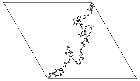
There are two discrete models for which convergence to $\mathrm{SLE}_{4}$ has been established by Scott Sheffield and the present author. These models are the harmonic explorer [80] and the interface of the discrete Gaussian free field [81]. The discrete and continuous Gaussian free fields (a.k.a. the harmonic crystal) play an important role in the heuristic physics analysis of various statistical physics models. The discrete Gaussian free field is a probability measure on real valued functions defined on a graph, often a piece of a lattice. If, for example, the graph is a triangulation of a domain in the plane, an interface is a curve in the dual graph separating vertices where the function is positive from vertices where the function is negative. See [85] or [81] for further details, and see Figure 7 for a simulation of the harmonic explorer, and therefore an approximation of $\mathrm{SLE}_{4}$.

Sheffield also announced work in progress connecting the Gaussian free field with $\mathrm{SLE}_{\kappa}$ for other values of $\kappa$. The basic idea is that while $\mathrm{SLE}_{4}$ may be thought of as a curve solving the equation $h=0$, where $h$ is the Gaussian free field, for other $\kappa$, the $\mathrm{SLE}_{\kappa}$ curve may be considered as a solution of

where $c$ is a constant depending on $\kappa$. When $\kappa=4$, the corresponding constant $c$ is zero, which reduces to the setting of [81]. Alternatively, (3) can be heuristically written as $c\,\gamma^{\prime}(s)=\exp(i\,h(\gamma(t))$, where $s$ is the length parameter of $\gamma$. However, we stress that it is hard to make sense of these equations, for the Gaussian free field is not a smooth function (in fact, it is not even a function but rather a distribution). Likewise, the SLE path is not rectifiable and its winding at most points is infinite.

As mentioned above, there are several different variants of SLE in simply connected domains: chordal, radial, as well as a few others, which we have not mentioned. These variants are rather closely related to one another [83]. There are also variants defined in the multiply-connected setting [101, 6, 5, 7]. One motivation for this study comes from statistical physics models, which are easy to define on multiply connected domains. Since one can easily vary the boundary conditions on different boundary components of the domain, it is clear that there is often more than one reasonable choice for the definition of the SLE path.

Finally, we mention an intriguing connection between Brownian motion and $\mathrm{SLE}_{\kappa}$ for $\kappa\in(8/3,4]$. There is the notion of the Brownian loop soup [63], which is a Poisson measure on the space of Brownian motion loops. According to [93], the boundaries of clusters of a sample from the loop soup measure with intensity $c$ are $\mathrm{SLE}_{\kappa}$-like paths, where $\kappa=\kappa(c)\in(8/3,4]$. The proof is to appear in a future joint work of Sheffield and Werner.

The above account describes some of the highlights of the developments in the field in the past several years. The rest of the paper will be devoted to a description of some problems where we hope to see some future progress. Some of these problems are obvious to anyone working in the field (though the solution is not obvious), while others are borrowed from several different sources. A few of the problems appear here for the first time. The paper [76] contains some additional problems.

To be precise, we must describe the meaning of these scaling limits. In fact, there are at least two distinct reasonable notions of convergence, which we now describe. Suppose that $\gamma_{n}$ are random paths in the closed upper half plane $\overline{\mathbb{H}}$ starting from $0$. Consider the one-point compactification $\hat{\mathbb{C}}={\mathbb{C}}\cup\{\infty\}$ of ${\mathbb{C}}={\mathbb{R}}^{2}$, which may be thought of as the sphere $S^{2}$. The law of $\gamma_{n}$ may be thought of as a Borel probability measure on the Hausdorff space of closed nonempty subsets of $\hat{\mathbb{C}}$. Since that Hausdorff space is compact, the space of Borel probability measures on it is compact with respect to weak convergence of measures [26]. We may say that $\gamma_{n}$ converges in the Hausdorff sense to a random set $\gamma\subset\overline{\mathbb{H}}\cup\{\infty\}$ if the law of $\gamma_{n}$ converges weakly to the law of $\gamma$. A similar definition applies to curves in the closure of a bounded domain $D\subset{\mathbb{C}}$. The above stated instances of convergence to SLE hold with respect to this notion. However, in the case of convergence to $\mathrm{SLE}_{8}$, this does not mean very much, for $\mathrm{SLE}_{8}$ fills up the domain.

The second notion of convergence is stronger. Suppose that each $\gamma_{n}$ is a.s. continuous with respect to the half-plane capacity parametrization from $\infty$. (This holds, in particular, if $\gamma_{n}$ is a.s. a [continuous] simple path.) If $d$ is a metric on $\hat{\mathbb{C}}={\mathbb{C}}\cup\{\infty\}$ compatible with its topology, then we may consider the metric

on the space of continuous paths defined on $[0,\infty)$. We may say that $\gamma_{n}$ converges to a random path $\gamma$ weakly-uniformly if the law of $\gamma_{n}$ converges weakly to the law of $\gamma$ in the space of Borel measures with respect to the metric $d^{*}$. This implies Hausdorff convergence. Since $d^{*}$ is finer than the Hausdorff metric, there are more functions from the space of paths to ${\mathbb{R}}$ that are continuous with respect to $d^{*}$ than with respect to the Hausdorff metric. Consequently, weakly-uniform convergence is stronger than Hausdorff convergence. In all the results stated above saying that some random path converges to SLE, the convergence is weakly-uniform when the paths are parametrized by capacity or half-plane capacity (depending on whether the convergence is to radial or chordal SLE, respectively).

In the following, when we ask for convergence to SLE, we will mean weakly-uniform convergence. However, weaker nontrivial forms of convergence would also be very interesting.

Let $G$ be either the square, the hexagonal or the triangular grid in the plane, positioned so that $0$ is some vertex in $G$. For $n\in{\mathbb{N}}$ consider the uniform measures on all self avoiding $n$-step walks in $G$ that start at $0$ and stay in the upper half plane. It has been shown in [60] that when $G={\mathbb{Z}}^{2}$ the limiting measure as $n\to\infty$ exists. (The same proof probably applies for the other alternatives for $G$, provided that $G$ is positioned so that horizontal lines through vertices in $G$ do not intersect the relative interior of edges of $G$ which they do not contain.)

The convergence may be considered with respect to either of the two topologies discussed in subsection 2.1.

In [60] some consequences of this convergence are indicated, as well as support for the conjecture.

There are some indications that the setting of the hexagonal lattice is easier: the rate of growth of the number of self avoiding paths on the hexagonal grid is predicted [72] to be $\bigl(2+\sqrt{2}+o(1)\bigr)^{n/2}$; no such prediction exists for the square grid or triangular lattice.

In dimensions $d>4$ Takashi Hara and Gordon Slade [32] proved that the scaling limit of self-avoiding random walk is Brownian motion. This is also believed to be the case for $d=4$. See [67] for references and further background on the self-avoiding walk.

There is a vast collection of height model interfaces that should converge to $\mathrm{SLE}_{4}$. The one theorem in this regard is the convergence of the interface of the Gaussian free field [81]. This was motivated by Kenyon’s theorem stating that the domino tiling height function converges to the Gaussian free field [42] and by Kenyon’s conjecture that the double domino interface converges to $\mathrm{SLE}_{4}$ (see [76] for a statement of this problem).

The domino height function is a function on ${\mathbb{Z}}^{2}$ associated with a domino tiling (see [42]). Its distribution is roughly (ignoring boundary issues) the uniform measure on functions $h:{\mathbb{Z}}^{2}\to{\mathbb{Z}}$ such that $h(0,0)=0$,

and $|h(z)-h(z^{\prime})|\in\{1,3\}$ if $|z-z^{\prime}|=1$, $z,z^{\prime}\in{\mathbb{Z}}^{2}$.

Let $D$ be a bounded domain in the plane whose boundary is a simple path in the triangular lattice, say. Let $\partial_{+}$ and $\partial_{-}$ be complementary arcs in $\partial D$ such that the two common endpoints of these arcs are midpoints of edges. Consider the uniform measure on functions $h$ taking odd integer values on vertices in $\overline{D}$ such that $h=1$ on $\partial_{+}$, $h=-1$ on $\partial_{-}$, and $|h(v)-h(u)|\in\{0,2\}$ for neighbors $v,u$. We may extend such a function $h$ to $\overline{D}$ by affine interpolation within each triangle, and this interpolation is consistent along the edges. There is then a unique connected path $\gamma$ that is the connected component of $h^{-1}(0)$ that contains the two endpoints of each of the two arcs $\partial_{\pm}$.

The convergence we expect for $h$ is in the same sense as in [42].

Note that if we restrict in the above the image of $h$ to be $\{1,-1\}$, we obtain critical site percolation on the triangular grid, and the limit of the corresponding interface is in this case $\mathrm{SLE}_{6}$.

Now suppose that $(D,\partial_{+},\partial_{-})$ is as above. Let $\lambda\in(0,1/2]$ be some constant and consider the uniform measure on functions $h$ taking real values on vertices in $\overline{D}$ such that $h=\lambda$ on $\partial_{+}$, $h=-\lambda$ on $\partial_{-}$ and $|h(v)-h(u)|\leq 1$ for every edge $[v,u]$.

In the case of the corresponding questions for the discrete Gaussian free field, there is just one constant $\lambda$ such that the interface converges to $\mathrm{SLE}_{4}$. For other choices of $\lambda$ the interface converges to a well-known variant of $\mathrm{SLE}_{4}$ [81].

There are some restricted classes of height models for which convergence to the Gaussian free field is known [71]. It may still be very hard to prove that the corresponding interface converges to $\mathrm{SLE}_{4}$. One interesting problem of this sort is the following.

The problem is natural, because the Gaussian free field is related to the Dirichlet Laplacian. In particular, the projections of the field onto the spaces spanned by eigenfunctions with eigenvalues in two disjoint intervals are independent.

The Ising model is a fundamental physics model for magnetism. Consider again a domain $D$ adapted to the triangular lattice and a partition $\partial D=\partial_{+}\cup\partial_{-}$ as in subsection 2.3. Now consider a function $h$ that take the values $\pm 1$ on vertices in $\overline{D}$ such that $h$ is $1$ on $\partial_{+}$ and $-1$ on $\partial_{-}$. On the collection of all such functions we put a probability measure such that the probability for a given $h$ is proportional to $e^{-2\beta k}$, where $\beta$ is a parameter and $k$ is the number of edges $[v,u]$ such that $h(v)\neq h(u)$. This is known as the Ising model and the value associate to a vertex is often called a spin. It is known that the critical value $\beta_{c}$ (which we do not define here in the context of the Ising model) for $\beta$ satisfies $e^{2\beta}=\sqrt{3}$ (see [69, 35]). Again, the interface at the critical $\beta=\beta_{c}$ is believed to converge to an SLE path, this time $\mathrm{SLE}_{3}$. For $\beta\in[0,\beta_{c})$ fixed, the interface should converge to $\mathrm{SLE}_{6}$. Note that when $\beta=0$, the model is again identical to critical site percolation on the triangular grid, and the interface does converge to $\mathrm{SLE}_{6}$.

When $\beta>\beta_{c}$ we do not expect convergence to SLE, and do not expect conformal invariance. The interface scaling limit is in this case a straight line segment if the domain is convex [75] (see also [29]).

The Fortuin-Kasteleyn [28] (FK) model (a.k.a. the random cluster model) is a probability measure on the collection of all subsets of the set of edges $E$ of a finite graph $G=(V,E)$. In the FK model, the measure of each $\omega\subset E$ is proportional to $\bigl(p/(1-p)\bigr)^{|\omega|}\,q^{c}$, where $q>0$ and $p\in(0,1)$ are parameters, $|\omega|$ is the cardinality of $\omega$, and $c$ is the number of connected components of the subgraph $(V,\omega)$. The FK model is very closely related to the well known Potts model [8], which is a generalization of the Ising model. Many questions about the Potts model can be translated to questions about the FK model and vice versa.

On the grid ${\mathbb{Z}}^{2}$, when $p=\sqrt{q}/(1+\sqrt{q})$ the FK model satisfies a form of self-duality.

The $O(n)$ loop model on a finite graph $G=(V,E)$ is a measure on the collection of subgraphs of $G$ where the degree of every vertex in the subgraph is $2$. (The subgraph does not need to contain all the vertices.) The probability of each such subgraph is proportional to $x^{e}\,n^{c}$, where $c$ is the number of connected components, $e$ is the number of edges in the subgraph, and $x,n>0$ are parameters. When $n$ is a positive integer, the $O(n)$ loop model is derived from the $O(n)$ spin model, which is a measure on the set of functions which associate to every vertex a unit vector in ${\mathbb{R}}^{n}$.

In order to pin down a specific long path in the $O(n)$ loop model, we pick two points on the boundary of the domain and require that in the random subgraph the degrees of two boundary vertices near these two points be $1$, while setting the degrees of all other boundary vertices to $0$, say. Then the measure is supported on configurations with one simple path and a collection of loops.

Now we specialize to the hexagonal lattice. Set $x_{c}(n):=\bigl(2+\sqrt{2-n}\bigr)^{-1/2}$, which is the conjectured critical parameter [72].

When $x<x_{c}(n)$, we expect the scaling limit to be a straight line segment (if the domain is convex). The fact that at $n=1$ we get the same limits as for the Ising model is no accident. It is not hard to see that the $O(1)$ loop measure coincides with the law of boundaries of Ising clusters. See [36] for further details.

Similar conjectures should hold in other lattices. However, the values of the critical parameters are expected to be different.

We now present an example of a discrete model where we suspect that perhaps conformal invariance might hold. However, we do not presently have a candidate for the scaling limit.

Fix $n\in{\mathbb{N}}_{+}$, and consider the collection of all trees contained in the grid $G$ that contain the origin and have $n$ vertices. Select a tree $T$ from this measure, uniformly at random.

It would be good to be able to produce some pictures. However, we presently do not know how to sample from this measure.

See [86] for background on lattice trees and for results in high dimensions and [17] for an analysis of a related continuum model.

It is natural to try to extend the understanding of percolation at $p_{c}$ to percolation at a parameter $p$ tending to $p_{c}$. One possible framework is as follows. Fix a parameter $q\in(0,1)$. Suppose that in Figure 3 with small mesh $\epsilon>0$ we choose $p(\epsilon)$ so that the probability to have a left to right crossing of white hexagons in some fixed $1\times 1$ square in the upper half plane is $q$ at percolation parameter $p=p(\epsilon)$. The corresponding interface will still be an unbounded path starting at $0$, but its distribution will be different from the interface at $p=1/2$ if $q\neq 1/2$. Thus, it is natural to ask

This problem is also very closely related to a problem formulated by F. Camia, L. Fontes and C. Newman [18].

Site percolation on the triangular lattice is only one of several different models for percolation in the plane. Among discrete models, widely studied is bond percolation on the square grid. As for site percolation on the triangular lattice, the critical probability is again $p_{c}=1/2$.

At present, Smirnov’s proof does not work for bond percolation on the square grid. The proof uses the invariance of the model under rotation by $2\,\pi/3$. Thus, the following problem presents itself.

Some progress on this problem has been reported by Vincent Beffara [9].

There are other natural percolation models which have been studied. Among them we mention Voronoi percolation and the boolean model. In Voronoi percolation one has two independent Poisson point processes in the plane, $W$ and $B$, with intensities $p$ and $1-p$, respectively. Let $\hat{W}$ be the closure of the set of points in ${\mathbb{R}}^{2}$ closer to $W$ than to $B$, and let $\hat{B}$ be the closure of the set of points closer to $B$. The set $\hat{W}$ is a sample from Voronoi percolation at parameter $p$. Some form of conformal invariance was proved for Voronoi percolation [14], but the version proved does not imply convergence to SLE. It is neither stronger nor weaker than the conformal invariance proved by Smirnov. Notable recent progress has been made for Voronoi percolation by Bollobás and Riordan [15], who established the very useful Russo-Seymour-Welsh theorem, as well as $p_{c}=1/2$ for Voronoi percolation.

The boolean percolation model (a.k.a. continuum percolation) can be defined by taking a Poisson set of points $W\subset{\mathbb{R}}^{2}$ of intensity $1$ and letting $\hat{W}$ be the set of points in the plane at distance at most $r$ from $W$. Here, $r$ is the parameter of the model. (Alternatively, one may fix $r=1$, say, and let the intensity of the Poisson process be the parameter, but this is essentially the same, by scaling.) The Russo-Seymour-Welsh theorem is known for this model [1, 77], but the critical value of the parameter has not been identified. A nice feature which the model shares with Voronoi percolation is invariance under rotations.

References

- [1] K. S. Alexander, The RSW theorem for continuum percolation and the CLT for Euclidean minimal spanning trees, Ann. Appl. Probab. 6 (1996), no. 2, 466–494.
- [2] O. Angel, Growth and percolation on the uniform infinite planar triangulation, Geom. Funct. Anal. 13 (2003), no. 5, 935–974.
- [3] , Scaling of Percolation on Infinite Planar Maps, I, 2005, arXiv:math.Pr/0501006.
- [4] M. T. Barlow, Fractals, and diffusion-limited aggregation, Bull. Sci. Math. 117 (1993), no. 1, 161–169.
- [5] R. O. Bauer and R. M. Friedrich, On radial stochastic Loewner evolution in multiply connected domains, 2004, arXiv:math.Pr/0412060.
- [6] , Stochastic Loewner evolution in multiply connected domains, C. R. Math. Acad. Sci. Paris 339 (2004), no. 8, 579–584.
- [7] , On Chordal and Bilateral SLE in multiply connected domains, 2005, arXiv:math.Pr/0503178.
- [8] R. J. Baxter, S. B. Kelland, and F. Y. Wu, Equivalence of the Potts model or Whitney polynomial with an ice-type model, J. Phys. A 9 (1976), 397–406.
- [9] V. Beffara, Critical percolation on other lattices, 2005, Talk at the Fields Institute, http://www.fields.utoronto.ca/audio/05-06/.
- [10] , The dimension of the SLE curves, 2002, arXiv:math.Pr/0211322.
- [11] , Cardy’s formula on the triangular lattice, the easy way, 2005, Preprint, http://www.umpa.ens-lyon.fr/˜vbeffara/files/Proceedings-Toronto.pdf.
- [12] V. Beffara and V. Sidoravicius, Percolation theory, 2005, arXiv:math.Pr/0507220.
- [13] I. Benjamini, G. Kalai, and O. Schramm, Noise sensitivity of Boolean functions and applications to percolation, Inst. Hautes Études Sci. Publ. Math. (1999), no. 90, 5–43 (2001).
- [14] I. Benjamini and O. Schramm, Conformal invariance of Voronoi percolation, Comm. Math. Phys. 197 (1998), no. 1, 75–107.
- [15] B. Bollobás and O. Riordan, The critical probability for random Voronoi percolation in the plane is 1/2, 2004, arXiv:math.Pr/0410336.
- [16] M. Bousquet-Melou and G. Schaeffer, The degree distribution in bipartite planar maps: applications to the Ising model, 2002, arXiv:math.CO/0211070.
- [17] D. C. Brydges and J. Z. Imbrie, Branched polymers and dimensional reduction, Ann. of Math. (2) 158 (2003), no. 3, 1019–1039.
- [18] F. Camia, L. R. G. Fontes, and C. M. Newman, The Scaling Limit Geometry of Near-Critical 2D Percolation, 2005, cond-mat/0510740.
- [19] F. Camia and C. M. Newman, The Full Scaling Limit of Two-Dimensional Critical Percolation, 2005, arXiv:math.Pr/0504036.
- [20] J. Cardy, Critical percolation in finite geometries, J. Phys. A 25 (1992), no. 4, L201–L206.
- [21] , SLE for theoretical physicists, Ann. Physics 318 (2005), no. 1, 81–118, cond-mat/0503313.
- [22] L. Carleson and N. Makarov, Aggregation in the plane and Loewner’s equation, Comm. Math. Phys. 216 (2001), no. 3, 583–607.
- [23] P. Chassaing and G. Schaeffer, Random planar lattices and integrated superBrownian excursion, Probab. Theory Related Fields 128 (2004), no. 2, 161–212.
- [24] M. den Nijs, A relation between the temperature exponents of the eight-vertex and the -state potts model, J. Phys. A 12 (1979), 1857–1868.
- [25] J. Dubédat, Excursion decompositions for SLE and Watts’ crossing formula, 2004, arXiv:math.Pr/0405074.
- [26] R. M. Dudley, Real analysis and probability, Wadsworth & Brooks/Cole Advanced Books & Software, Pacific Grove, CA, 1989.
- [27] B. Duplantier and K.-H. Kwon, Conformal invariance and intersection of random walks, Phys. Rev. Let. (1988), 2514–2517.
- [28] C. M. Fortuin and P. W. Kasteleyn, On the random-cluster model. I. Introduction and relation to other models, Physica 57 (1972), 536–564.
- [29] L. Greenberg and D. Ioffe, On an invariance principle for phase separation lines, Ann. Inst. H. Poincaré Probab. Statist. 41 (2005), no. 5, 871–885.
- [30] G. Grimmett, Percolation, second ed., Grundlehren der Mathematischen Wissenschaften [Fundamental Principles of Mathematical Sciences], vol. 321, Springer-Verlag, Berlin, 1999.
- [31] O. Häggström, Y. Peres, and J. E. Steif, Dynamical percolation, Ann. Inst. H. Poincaré Probab. Statist. 33 (1997), no. 4, 497–528.
- [32] T. Hara and G. Slade, Self-avoiding walk in five or more dimensions. I. The critical behaviour, Comm. Math. Phys. 147 (1992), no. 1, 101–136.
- [33] T. E. Harris, A lower bound for the critical probability in a certain percolation process, Proc. Cambridge Philos. Soc. 56 (1960), 13–20.
- [34] M. B. Hastings and L. S. Levitov, Laplacian growth as one-dimensional turbulence, Physica D 116 (1998), 244–252.
- [35] C. Itzykson and J.-M. Drouffe, Statistical field theory. Vol. 1, Cambridge Monographs on Mathematical Physics, Cambridge University Press, Cambridge, 1989, From Brownian motion to renormalization and lattice gauge theory.
- [36] W. Kager and B. Nienhuis, A guide to stochastic Löwner evolution and its applications, J. Statist. Phys. 115 (2004), no. 5-6, 1149–1229, math-ph/0312056.
- [37] G. Kalai and S. Safra, Threshold phenomena and influence, Computational Complexity and Statistical Physics (New York) (G. I. A.G. Percus and C. Moore, eds.), Oxford University Press, 2005, http://www.ma.huji.ac.il/˜kalai/ML.pdf.
- [38] T. Kennedy, Monte Carlo comparisons of the self-avoiding walk and SLE as parameterized curves, 2005, arXiv:math.Pr/0510604.
- [39] R. Kenyon, The asymptotic determinant of the discrete Laplacian, Acta Math. 185 (2000), no. 2, 239–286.
- [40] , Conformal invariance of domino tiling, Ann. Probab. 28 (2000), no. 2, 759–795.
- [41] , Long-range properties of spanning trees, J. Math. Phys. 41 (2000), no. 3, 1338–1363, Probabilistic techniques in equilibrium and nonequilibrium statistical physics.
- [42] , Dominos and the Gaussian free field, Ann. Probab. 29 (2001), no. 3, 1128–1137.
- [43] H. Kesten, The critical probability of bond percolation on the square lattice equals , Comm. Math. Phys. 74 (1980), no. 1, 41–59.
- [44] , Upper bounds for the growth rate of DLA, Phys. A 168 (1990), no. 1, 529–535.
- [45] , Some highlights of percolation, Proceedings of the International Congress of Mathematicians, Vol. I (Beijing, 2002) (Beijing), Higher Ed. Press, 2002, pp. 345–362.
- [46] V. G. Knizhnik, A. M. Polyakov, and A. B. Zamolodchikov, Fractal structure of D-quantum gravity, Modern Phys. Lett. A 3 (1988), no. 8, 819–826.
- [47] G. Kozma, Scaling limit of loop erased random walk - a naive approach, 2002, arXiv:math.Pr/0212338.
- [48] , The scaling limit of loop-erased random walk in three dimensions, 2005, arXiv:math.Pr/0508344.
- [49] R. Langlands, P. Pouliot, and Y. Saint-Aubin, Conformal invariance in two-dimensional percolation, Bull. Amer. Math. Soc. (N.S.) 30 (1994), no. 1, 1–61, arXiv:math.MP/9401222.
- [50] G. F. Lawler, The dimension of the frontier of planar Brownian motion, Electron. Comm. Probab. 1 (1996), no. 5, 29–47 (electronic).
- [51] , A self-avoiding random walk, Duke Math. J. 47 (1980), no. 3, 655–693.
- [52] , Conformally invariant processes in the plane, Mathematical Surveys and Monographs, vol. 114, American Mathematical Society, Providence, RI, 2005.
- [53] G. F. Lawler, O. Schramm, and W. Werner, Values of Brownian intersection exponents. I. Half-plane exponents, Acta Math. 187 (2001), no. 2, 237–273, arXiv:math.PR/9911084.
- [54] , Values of Brownian intersection exponents. II. Plane exponents, Acta Math. 187 (2001), no. 2, 275–308, arXiv:math.PR/0003156.
- [55] , Values of Brownian intersection exponents. III. Two-sided exponents, Ann. Inst. H. Poincaré Probab. Statist. 38 (2002), no. 1, 109–123.
- [56] , One-arm exponent for critical 2D percolation, Electron. J. Probab. 7 (2002), no. 2, 13 pp. (electronic).
- [57] , Sharp estimates for Brownian non-intersection probabilities, In and out of equilibrium (Mambucaba, 2000), Progr. Probab., vol. 51, Birkhäuser Boston, Boston, MA, 2002, pp. 113–131.
- [58] , Conformal restriction: the chordal case, J. Amer. Math. Soc. 16 (2003), no. 4, 917–955 (electronic).
- [59] , Conformal invariance of planar loop-erased random walks and uniform spanning trees, Ann. Probab. 32 (2004), no. 1B, 939–995, arXiv:math.PR/0112234.
- [60] , On the scaling limit of planar self-avoiding walk, Fractal geometry and applications: a jubilee of Benoît Mandelbrot, Part 2, Proc. Sympos. Pure Math., vol. 72, Amer. Math. Soc., Providence, RI, 2004, pp. 339–364.
- [61] G. F. Lawler and W. Werner, Intersection exponents for planar Brownian motion, Ann. Probab. 27 (1999), no. 4, 1601–1642.
- [62] , Universality for conformally invariant intersection exponents, J. Eur. Math. Soc. (JEMS) 2 (2000), no. 4, 291–328.
- [63] , The Brownian loop soup, Probab. Theory Related Fields 128 (2004), no. 4, 565–588, math-PR/0304419.
- [64] P. Lévy, Processus Stochastiques et Mouvement Brownien. Suivi d’une note de M. Loève, Gauthier-Villars, Paris, 1948.
- [65] K. Löwner (C. Loewner), Untersuchungen über schlichte konforme abbildungen des einheitskreises, i, Math. Ann. 89 (1923), 103–121.
- [66] R. Lyons, A bird’s-eye view of uniform spanning trees and forests, Microsurveys in discrete probability (Princeton, NJ, 1997), Amer. Math. Soc., Providence, RI, 1998, pp. 135–162.
- [67] N. Madras and G. Slade, The self-avoiding walk, Probability and its Applications, Birkhäuser Boston Inc., Boston, MA, 1993.
- [68] J. F. Marckert and A. Mokkadem, Limit of Normalized Quadrangulations: the Brownian map, 2004, arXiv:math.Pr/0403398.
- [69] B. M. McCoy and T. T. Wu, The two-dimensional Ising model, Harvard University Press, Cambridge, Mass., 1973.
- [70] R. Meester and R. Roy, Continuum percolation, Cambridge Tracts in Mathematics, vol. 119, Cambridge University Press, Cambridge, 1996.
- [71] A. Naddaf and T. Spencer, On homogenization and scaling limit of some gradient perturbations of a massless free field, Comm. Math. Phys. 183 (1997), no. 1, 55–84.
- [72] B. Nienhuis, Exact critical point and critical exponents, Phys. Rev. Let. 49 (1982), 1062–1065.
- [73] , Coulomb gas description of 2-d critical behaviour, J. Stat. Phys. 34 (1984), 731–761.
- [74] R. Pemantle, Choosing a spanning tree for the integer lattice uniformly, Ann. Probab. 19 (1991), no. 4, 1559–1574.
- [75] C.-E. Pfister and Y. Velenik, Interface, surface tension and reentrant pinning transition in the D Ising model, Comm. Math. Phys. 204 (1999), no. 2, 269–312.
- [76] S. Rohde and O. Schramm, Basic properties of SLE, Ann. of Math. (2) 161 (2005), no. 2, 883–924.
- [77] R. Roy, The Russo-Seymour-Welsh theorem and the equality of critical densities and the “dual” critical densities for continuum percolation on , Ann. Probab. 18 (1990), no. 4, 1563–1575.
- [78] L. Russo, A note on percolation, Z. Wahrscheinlichkeitstheorie und Verw. Gebiete 43 (1978), no. 1, 39–48.
- [79] O. Schramm, Scaling limits of loop-erased random walks and uniform spanning trees, Israel J. Math. 118 (2000), 221–288.
- [80] O. Schramm and S. Sheffield, Harmonic explorer and its convergence to , Ann. Probab. 33 (2005), no. 6, 2127–2148.
- [81] , Contour lines of the 2D Gaussian free field, 2006, In preparation.
- [82] O. Schramm and J. E. Steif, Quantitative noise sensitivity and exceptional times for percolation, 2005, arXiv:math.Pr/0504586.
- [83] O. Schramm and D. B. Wilson, SLE coordinate changes, New York J. Math. 11 (2005), 659–669, http://nyjm.albany.edu:8000/j/2005/11-31.html.
- [84] P. D. Seymour and D. J. A. Welsh, Percolation probabilities on the square lattice, Ann. Discrete Math. 3 (1978), 227–245, Advances in graph theory (Cambridge Combinatorial Conf., Trinity College, Cambridge, 1977).
- [85] S. Sheffield, Gaussian free fields for mathematicians, 2003, arXiv:math.Pr/0312099.
- [86] G. Slade, Lattice trees, percolation and super-Brownian motion, Perplexing problems in probability, Progr. Probab., vol. 44, Birkhäuser Boston, Boston, MA, 1999, pp. 35–51.
- [87] S. Smirnov, Critical percolation in the plane: conformal invariance, Cardy’s formula, scaling limits, C. R. Acad. Sci. Paris Sér. I Math. 333 (2001), no. 3, 239–244.
- [88] S. Smirnov and W. Werner, Critical exponents for two-dimensional percolation, 2001, To appear in Math. Research Letters, arXiv:math.Pr/0109120.
- [89] S. J. Taylor, The measure theory of random fractals, Math. Proc. Cambridge Philos. Soc. 100 (1986), no. 3, 383–406.
- [90] B. Tsirelson, Fourier-Walsh coefficients for a coalescing flow (discrete time), TAU RP-SOR-99-02, 1999, arXiv:math.Pr/9903068.
- [91] , Scaling limit of Fourier-Walsh coefficients (a framework), TAU RP-SOR-99-04, 1999, arXiv:math.Pr/9903121.
- [92] G. M. T. Watts, A crossing probability for critical percolation in two dimensions, J. Phys. A 29 (1996), no. 14, L363–L368.
- [93] W. Werner, SLEs as boundaries of clusters of Brownian loops, C. R. Math. Acad. Sci. Paris 337 (2003), no. 7, 481–486, arXiv:math.PR/0308164.
- [94] , Random planar curves and Schramm-Loewner evolutions, Lectures on probability theory and statistics, Lecture Notes in Math., vol. 1840, Springer, Berlin, 2004, pp. 107–195, arXiv:math.PR/0303354.
- [95] , Conformal restriction and related questions, Probab. Surv. 2 (2005), 145–190 (electronic).
- [96] , The conformally invariant measure on self-avoiding loops, 2005, arXiv:math.Pr/0511605.
- [97] , Conformal restriction properties, Proceedings of the Madrid ICM 2006, 2006, To appear.
- [98] J. C. Wierman, Bond percolation on honeycomb and triangular lattices, Adv. in Appl. Probab. 13 (1981), no. 2, 298–313.
- [99] D. B. Wilson, Generating random spanning trees more quickly than the cover time, Proceedings of the Twenty-eighth Annual ACM Symposium on the Theory of Computing (Philadelphia, PA, 1996) (New York), ACM, 1996, pp. 296–303.
- [100] T. A. Witten and L. M. Sander, Diffusion-limited aggregation, Phys. Rev. B (3) 27 (1983), no. 9, 5686–5697.
- [101] D. Zhan, Stochastic Loewner evolution in doubly connected domains, Probab. Theory Related Fields 129 (2004), no. 3, 340–380, arXiv:math.PR/0310350.
- [102] R. M. Ziff, Exact critical exponent for the shortest-path scaling function in percolation, J. Phys. A 32 (1999), no. 43, L457–L459.