[francisco.santos@unican.es, URL: http://personales.unican.es/santosf/]Francisco Santos, Departamento de Matemáticas, Estadística y Computación, Universidad de Cantabria, E-39005 Santander, SPAIN
rimary 52B11; Secondary 52B20
Geometric bistellar flips. The setting, the context and a construction
Abstract
We give a self-contained introduction to the theory of secondary polytopes and geometric bistellar flips in triangulations of polytopes and point sets, as well as a review of some of the known results and connections to algebraic geometry, topological combinatorics, and other areas.
As a new result, we announce the construction of a point set in general position with a disconnected space of triangulations. This shows, for the first time, that the poset of strict polyhedral subdivisions of a point set is not always connected.
keywords
Triangulation, point configuration, bistellar flip, polyhedral subdivision, disconnected flip-graph.Classification:
PIntroduction
Geometric bistellar flips are “elementary moves”, that is, minimal changes, between triangulations of a point set in affine space . In their present form they were introduced around 1990 by Gel’fand, Kapranov and Zelevinskii during their study of discriminants and resultants for sparse polynomials [26, 27]. Not surprisingly, then, these bistellar flips have several connections to algebraic geometry. For example, the author’s previous constructions of point sets with a disconnected graph of triangulations in dimensions five and six [60, 63] imply that certain algebraic schemes considered in the literature [3, 12, 31, 53], including the so-called toric Hilbert scheme, are sometimes not connected.
Triangulations of point sets play also an obvious role in applied areas such as computational geometry or computer aided geometric design, where a region of the plane or 3-space is triangulated in order to approximate a surface, answer proximity or visibility questions, etc. See, for example, the survey articles [7, 9], or [23]. In these fields, flips between triangulations have also been considered since long [38]. Among other things, they are used as the basic step to compute an optimal triangulation of a point set incrementally, that is, adding the points one by one. This incremental flipping algorithm is the one usually preferred for, for example, computing the Delaunay triangulation, as “the most intuitive and easy to implement” [7], and yet as efficient as any other.
In both the applied and the theoretical framework, the situation is the same: a fixed set of points is given to us (the “sites” for a Delaunay triangulation computation, the test points for a surface reconstruction, or a set of monomials, represented as points in , in the algebro-geometric context) and we need to either explore the collection of all possible triangulations of this set or search for a particular one that satisfies certain optimality properties. Geometric bistellar flips are the natural way to do this. For this reason, it was considered one of the main open questions in polytope theory ten years ago whether point sets exist with triangulations that cannot be connected via these flips [76]. As we have mentioned above, this question was answered negatively by the author of this paper, starting in dimension 5. The question is still open in dimensions three and four.
This paper intends to be an introduction to this topic, organized in three parts.
The first section is a self-contained introduction to the theory of geometric bistellar flips and secondary polytopes in triangulations of point sets, aimed at the non-expert. The results in it are certainly not new (most come from the original work of Gel’fand, Kapranov and Zelevinskii mentioned above) but the author wants to think that this section has some expository novelty; several examples that illustrate the theory are given, and our introduction of geometric bistellar flips first as certain polyhedral subdivisions and only afterwards as transformations between triangulations is designed to show that the definition is as natural as can be. This section finishes with an account of the state-of-the-art regarding knowledge of the graph of flips for sets with “few” points or “small” dimension, with an emphasis on the differences between dimensions two and three.
The second section develops in more detail the two contexts in which we have mentioned that flips are interesting (computational geometry and algebraic geometry) together with other two, that we call “combinatorial topology” and “topological combinatorics”. Combinatorial topology refers to the study of topological manifolds via triangulations of them. Bistellar flips have been proposed as a tool for manifold recognition [17, 42], and triangulations of the 3-sphere without bistellar flips other than “insertion of new vertices” are known [22]. Topological combinatorics refers to topological methods in combinatorics, particularly to the topology of partially ordered sets (posets) via their order complexes. The graph of triangulations of a point set consists of the first two levels in the poset of polyhedral subdivisions of , which in turn is just an instance of several similar posets studied in combinatorics with motivations and applications ranging from oriented matroid theory to bundle theories in differential geometry.
The third section announces for the first time the construction of a point set in general position whose graph of triangulations is not connected. The details of the proof appear in [64]. The point set is also the smallest one known so far to have a disconnected graph of flips.
Theorem
There is a set of 17 points in general position in whose graph of triangulations is not connected.
As usual in geometric combinatorics, a finite point set is said to be in general position if no of the points lie in an affine hyperplane. Equivalently, if none of the determinants defined by the point set vanish. Point sets in general position form an open dense subset in the space of sets of dimension with elements. That is to say, “random point sets” are in general position. Point sets that are not in general position are said to be in special position.
The connectivity question has received special attention in general position even before disconnected examples in special position were found. For example, Challenge 3 in [76] and Problem 28 in [46] specifically ask whether disconnected graphs of flips exist for point sets in special position (the latter asks this only for dimension 3). Although it was clear (at least to the author of this paper) from the previous examples of disconnected graphs of flips that examples in general position should also exist, modifying those particular examples to general position and proving that their flip-graphs are still not connected is not an easy task for quite intrinsic reasons: the proofs of non-connectednes in [60, 63] are based on the fact that the point sets considered there are cartesian products of lower dimensional ones.
In our opinion, an example of a disconnected graph of flips in general position is interesting for the following three reasons:
- 1.
The definition of flip that is most common in computational geometry coincides with ours (which is the standard one in algebraic geometry and polytope combinatorics) only for point sets in general position. In special position, the computational geometric definition is far more restrictive and, in particular, taking it makes disconnected graphs of flips in special position be “no surprise”. For example, Edelsbrunner [23] says that the flip-graph among the (three) triangulations of a regular octahedron is not connected; see Section 2.1.
- 2.
Leaving aside the question of definition, in engineering applications the coordinates of points are usually approximate and there is no loss in perturbing them into general position. That is, the general position case is sometimes the only case.
- 3.
Even in a purely theoretical framework, point sets in general position have somehow simpler properties than those in special position. If a point set in special position has a non-connected graph of flips then automatically some subset of (perhaps itself) has a disconnected poset of subdivisions. This poset is sometimes called the Baues poset of and its study is (part of) the so-called generalized Baues problem. See Section 2.3, or [57] for more precise information on this. In partiular, the present example is the first one (proven) to have a disconnected Baues poset.
Corollary
There is a set of at most 17 points in whose poset of proper polyhedral subdivisions is not connected.
1 The setting
1.1 Triangulations. Regular triangulations and subdivisions
Triangulations and polyhedral subdivisions
A (convex) polytope is the convex hull of a finite set of points in the affine space . A face of is its intersection with any hyperplane that does not cross the relative interior of . (Here, the relative interior of is the interior of regarded as a subset of its affine span). We remind the reader that the faces of dimensions and of a -polytope are called vertices, edges, ridges and facets, respectively. Vertices of form the minimal such that .
A -simplex is a polytope whose vertices (necessarily ) are affinely independent. It has faces of each dimension , which are all simplices.
Definition 1.1.
Let be a finite point set in . A triangulation of is any collection of affinely spanning and affinely independent subsets of with the following properties:
- 1.
if and are in , then is a face of both and . That is, induces a geometric simplicial complex in ;
- 2.
. That is, covers the convex hull of .
Note that our definition allows for some points of not to be used at all in a particular triangulation. Extremal points (vertices of ) are used in every triangulation. The elements of a triangulation are called cells.
We can define polyhedral subdivisions of by removing the requirement of the sets to be affinely independent in Definition 1.1. Since a general subset of may contain points which are not vertices of , now the fact that the elements of a subdivision are subsets of rather than “subpolytopes” is not just a formality: points which are not vertices of any “cell” in the subdivision may still be considered “used” as elements of some cells. In order to get a nicer concept of polyhedral subdivision, we also modify part 1 in Definition 1.1, adding the following (redundant for affinely independent sets) condition:
That is, if contains some point in the common face of and but not a vertex of it, that point is either in both or in none of and .
Polyhedral subdivisions of form a partially ordered set (or poset) with respect to the following refinement relation:
Triangulations are, of course, the minimal elements in this poset. The poset has a unique maximal element, namely the trivial suvdivision .
Example 1.2.
Let be the following set of five points in the plane. We take the convention that points are displayed as columns in a matrix, and that an extra homogenization coordinate (the row of 1’s in the following matrix) is added so that linear algebra, rather than affine geometry, can be used for computations:
| (1) |
The following are the nine polyhedral subdivisions of . Arrows represent the refinement relation, pointing from the coarser to the finer subdivision. For clarity, we write “” meaning , and so on. Figure 1 shows pictures of the subdivisions. In the corners are the four triangulations of and in the middle is the trivial subdivision.
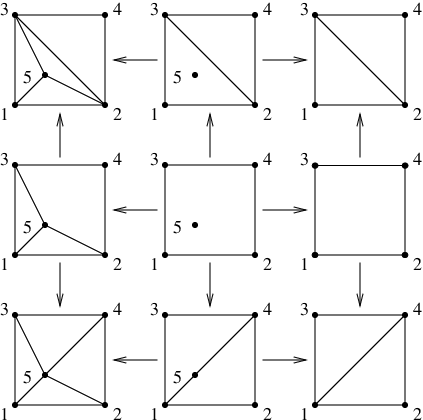
The last two columns of subdivisions geometrically induce the same decomposition of into subpolygons. Still, we consider them different subdivisions since the middle column “uses” the interior point while the right column does not.
Regular subdivisions
Let a point set be given, and choose a function to lift to as the point set
A lower facet of is a facet whose supporting hyperplane lies below the interior of . The following is a polyhedral subdivision of , where is the projection that forgets the last coordinate:
Geometrically, we are projecting down onto the lower envelope of , keeping track of points that lie in the lower boundary even if they are not vertices of a facet.
Definition 1.3.
The polyhedral subdivisions and triangulations that can be obtained in this way are called regular.
If is sufficiently generic then is clearly a triangulation. Regular triangulations are particularly simple and yet quite versatile. They appear in different contexts under different names such as coherent [27], convex [34, 73], Gale [45], or generalized (or, weighted) Delaunay [23] triangulations. The latter refers to the fact that the Delaunay triangulation of , probably the most used triangulation in applications, is the regular triangulation obtained with , where is the euclidean norm.
Example 1.4.
Let
This is a configuration of six points in the affine plane with equation in . Since the matrix is already homogeneous (meaning precisely that columns lie in an affine hyperplane) we do not need the extra homogenization row. The configuration consists of two parallel equilateral triangles, one inside the other. We leave it to the reader to check that the following are two non-regular triangulations (see Figure 2):

This example is the smallest possible, since 1-dimensional point configurations and point configurations with at most points in any dimension only have regular triangulations. The former is easy to prove and the latter was first shown in [40]. The earliest appearance of these two non-regular triangulations that we know of is in [18], although they are closely related to Schönhardt’s classical example of a non-convex 3-polytope that cannot be triangulated [65].11 1 We describe Schönhardt’s polyhedron and its relation to this example in Example 1.23.
Remark 1.5.
Suppose that two point sets and have the same oriented matroid [16], or order type. This means that for every subset of labels, the determinants of the point sets and have the same sign.22 2 Observe that the bijection between and implicit by the labels is part of the defintion. It is an easy exercise to check that then and have the same triangulations and subdivisions.33 3 More precisely, the implicit bijection between and induces a bijection between their polyhedral subdivisions. However, they do not necessarily have the same regular subdivisions. For example, the points of example 1.4 are in general position and, hence, their oriented matroid does not change by a small perturbation of coordinates. But any sufficiently generic perturbation makes one of the two non-regular triangulations and become regular.
Still, the following is true [61]: the existence of non-regular triangulations of depends only on the oriented matroid of .
The secondary polytope
Let denote the space of all lifting functions on a certain point set with elements. In principle is isomorphic to in an obvious way; but we mod-out functions that lift all of to a hyperplane, because adding one of them to a given lifting function does not (combinatorially) change the lower envelope of . We call these particular lifting functions affine. They form a linear subspace of dimension of . Hence, after we mod-out affine functions we have .
For a given polyhedral subdivision of , the subset of consisting of functions that produce , is a (relatively open) polyhedral cone; that is, it is defined by a finite set of linear homogeneous equalities and strict inequalities. Equalities appear only if is not a triangulation and express the fact that if is not affinely independent then must lift all to lie in a hyperplane. Inequalities express the fact that for each and point , is lifted above the hyperplane spanned by the lifting of .
The polyhedral cones obtained for different choices of are glued together forming a polyhedral fan, that is, a “cone over a polyhedral complex”, called the secondary fan of . The prototypical example of a fan is the normal fan of a polytope, whose cones are the exterior normal cones of different faces of . A seminal result in the theory of triangulations of polytopes is that the secondary fan is actually polytopal; that is, it is the normal fan of a certain polytope:
Theorem 1.6 (Gel’fand-Kapranov-Zelevinskii [26, 27]).
For every point set of points affinely spanning there is a polytope in whose normal fan is the secondary fan of .
In particular, the poset of regular subdivisions of is isomorphic to the poset of faces of . Vertices correspond to regular triangulations and itself (which is, by convention, considered a face) corresponds to the trivial subdivision. The polytope is called the secondary polytope of .
There are two standard ways to construct the secondary polytope of a point set .44 4 Polytopality of a fan is equivalent to the feasibility of a certain system of linear equalities and strict inequalities. But here we mean more direct and intrinsic constructions of the secondary polytope. The original one, by Gel’fand, Kapranov and Zelevinskii [26, 27] gives, for each regular triangulation of , coordinates of the corresponding vertex of in terms of the volumes of simplices incident in to each point of .
The second one, by Billera and Sturmfels [13], describes the whole polytope as the Minkowski integral of the fibers of the affine projection , where is a simplex with vertices (hence, of dimension ) and bijects the vertices of to (see Theorem thm:fiber).
Example 1.7.
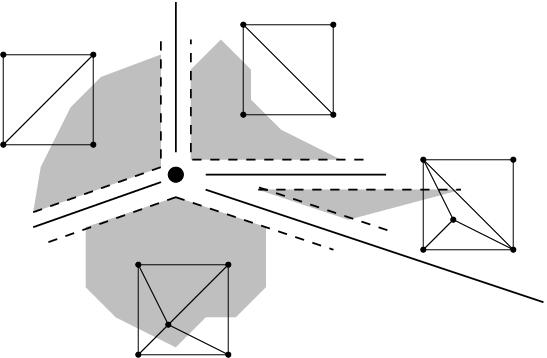
(Example 1.2 continued) Figure 3 shows the secondary fan of the five points. To mod-out affine functions we have taken , and the horizontal and vertical coordinates in the figure give the values of and , respectively. The triangulation corresponding to each two-dimensional cone is displayed.
Example 1.8.
(Example 1.4 continued) The secondary polytope of this point set is 3-dimensional, and contains a hexagonal face corresponding to the regular subdivision
This regular subdivision can be refined to a triangulation in eight ways, by independently inserting a diagonal in the quadrilaterals , and . Six of these triangulations are regular, and correspond to the vertices of the hexagon. The other two, and , are non-regular and they “lie” in the center of the hexagon.
We have mentioned that if the point set is perturbed slightly then one of the triangulations becomes regular. What happens in the secondary polytope is the following: the perturbation “inflates” the hexagon so that the eight points (the vertices of the hexagon and the two interior points representing and ) become, combinatorially, the vertices of a cube. The points corresponding to and move in opposite directions, one of them going to the interior of the secondary polytope and the other becoming a new vertex of it. The hexagonal face gets refined into three quadrilaterals. Of course, the vertices of the hexagon also move in the process, and are no longer coplanar.
Example 1.9.
(The convex -gon and the associahedron) All triangulations of a convex -gon are regular and their number is the nd Catalan number
The corresponding secondary polytope is called the associahedron. The name comes from the fact that there is a bijection between triangulations of the -gon and the ways to put the parentheses in an associative product of factors.
The associahedron is a classical object in combinatorics, first studied55 5 As a combinatorial cell complex, without an explicit polytopal realization. by Stasheff and Tamari [72, 68]. It was shown to be polytopal by Haiman (unpublished) and Lee [39]. That its diameter equals “for every sufficiently big ’’66 6 Sleator et al. do not say “how big” is “sufficiently big” in their statement, but conjecture that is enough. We consider this an interesting and somehow shameful open question. was shown by Sleator, Tarjan and Thurston [67], with motivations coming from theoretical computer science and tools from hyperbolic geometry.
Remark 1.10.
In Sections 2.3 and 2.4 we will mention triangulations of a set of vectors rather than points. They are defined exactly as triangulations of point sets, just changing the word “affinely” to “linearly” and the operator “” to “” (“positive span”) in Definition 1.1. Put differently, a triangulation of a vector set is a simplicial fan covering and whose rays are in the positive directions of (not necessarily all) the elements of . Equivalently, and perhaps closer to readers familiar with classical geometry, we can, without loss of generality, normalize all vectors of to lie in the unit sphere . Then, triangulations of are the geodesic triangulations, with vertices contained in , of the spherical convex hull of .
The existence and properties of regular subdivisions and secondary fans (and of the bistellar flips introduced in the next section) generalize almost without change to vector configurations.77 7 Although with one notable difference. For a general vector configuration not every function produces a lift with a well-defined “lower envelope”. Only the functions that do, namely those for which a linear hyperplane exists containing or lying below all the lifted vectors, define a regular polyhedral subdivision. These functions form a cone in . The secondary fan is still well-defined but, of course, it cannot be the normal fan of a polytope. It is, however, the normal fan of an unbounded convex polyhedron, called the secondary polyhedron of [11].
1.2 Geometric bistellar flips
Flips as polyhedral subdivisions
In order to introduce the notion of local move (flip) between triangulations of , we use the secondary fan as a guiding light: whatever our definition is, restricted to regular triangulations a flip should correspond to crossing a “wall” between two full-dimensional cones in the secondary fan; that is, a flip between two regular triangulations and can be regarded as certain regular subdivision with the property that its only two regular refinements are precisely and . Some thought will convince the reader that the necessary and sufficient condition for a lifting function to produce a with this property is that there is a unique minimal affinely dependent subset in whose lifting is contained in some lower facet of the lifted point set . This leads to the following simple, although perhaps not very practical, definition.
Definition 1.11.
Let be a (not-necessarily regular) subdivision of a point set . We say that is a flip if there is a unique affinely dependent subset contained in some cell of .
Lemma 1.12.
If is a flip, then there are exactly two proper refinements of , which are both triangulations.
Proof 1.13.
Let be a refinement of . Let be the unique affinely dependent subset of contained in some cell of . Each cell of containing gets refined in , while each cell not containing is also a cell in .
The statement then follows from the understanding of the combinatorics of point sets with a unique affinely dependent subset . Let be such a point set. Each point in is affinely independent of the rest, so is an “iterated cone” over . In particular, there is a face of such that and every refinement of consists of a refinement of coned to the points of . Moreover, all cells of containing must have refined the same way, so that there is a bijection between the refinements of and the polyhedral subdivisions of , as a point set. The result then follows from the fact (see below) that a minimal affinely dependent set has exactly three subdivisions: the trivial one and two triangulations.
This lemma allows us to understand a flip, even in the non-regular case, as a relation or a transformation between its two refinements. This is the usual usage of the word “flip”, and our next topic.
Flips as elementary changes
A minimal affinely dependent set is called a circuit in geometric combinatorics. The points in a circuit satisfy a unique (up to a constant) affine dependence equation with , and all the must be non zero (or otherwise is not minimally dependent). This affine dependence implicitly decomposes into two subsets
The pair is usually called a signed or oriented circuit. We will slightly abuse notation and speak of “the circuit ”, unless we need to emphasize the distinction between the set (the support of the circuit) and its partition.
A more geometric description is that is the only partition of into two subsets whose convex hulls intersect, and that they intersect in their relative interiors. This is usually called Radon’s property [54] and the oriented circuit a Radon partition.
Spanning and affinely independent subsets of are all the sets of the form . Moreover, by Radon’s property two such sets and can be cells in the same triangulation of if and only if and lie in the same side of the partition. In other words:
Lemma 1.14.
A circuit has exactly two triangulations:
This leads to a second definition of flip, equivalent to Definition 1.11, but more operational. This is the definition originally devised by Gel’fand, Kapranov and Zelevinskii [27]. The link of a set in a triangulation of is defined as
Definition 1.15.
Let be a triangulation of a point set . Suppose that contains one of the triangulations, say , of a circuit . Suppose also that all cells have the same link in , and call it .
Then, we say that supports a geometric bistellar flip (or a flip, for short) in and that the following triangulation of is obtained from by this flip:
If and we say that the flip is of type . Flips of types and are called, insertion and deletion flips, since they add or remove a vertex in the triangulation.
The graph of flips of has as vertices all the triangulations of and as edges the geometric bistellar flips between them.
Of course, an flip can always be reversed, giving a flip. The reason for the words “geometric bistellar” in our flips can be found in Section 2.2.
Example 1.16.
(Examples 1.2 and 1.7 continued) The change between the two top triangulations in Figure 3 is a flip, as is the change between the two bottom ones. The flip from the top-right to the bottom-right is a flip (“1 triangle disappears and 3 are inserted”) and the flip from the top-left to the bottom-left is a flip (“one edge is removed, together with its link, and two are inserted, with the same link”). The latter is supported in the circuit formed by the three collinear points.
We omit the proof of the following natural statement.
Theorem 1.17.
The following two facts are proved in [61]:
Remark 1.18.
- 1.
If all proper refinements of a subdivision are triangulations, then has exactly two of them and is a flip. That is to say, flips are exactly the “next-to-minimal” elements in the refinement poset of all subdivisions of .
- 2.
Every non-regular subdivision can be refined to a non-regular triangulation [60]. In particular, not only edges of the secondary polytope correspond to flips between two regular triangulations, but also every flip between two regular triangulations corresponds to an edge.
Detecting flips
Definitions 1.11 and 1.15 are both based on the existence of a flippable circuit with certain properties. But in order to detect flips only some circuits need to be checked:
Lemma 1.19.
Every flip in a triangulation other than an insertion flip is supported in a circuit contained in the union of two adjacent cells of .
Observe that the circuit contained in two adjacent cells always exists and is unique. Also, that the insertion flips left aside in this statement are easy to detect:88 8 We mean, theoretically. Algorithmically, insertion flips are far from trivial since they imply locating the simplex of that contains the point to be inserted, which takes about the logarithm of the number of simplices in . This is very expensive, since algorithms in computational geometry that use flipping in triangulations usually are designed to take constant time per flip other than an insertion flip. See Section 2.1. There is one for each point not used in , that inserts the point by subdividing the minimum (perhaps not full-dimensional) simplex such that . The flippable circuit is .
Proof 1.20.
Let be a circuit that supports a flip in , with . Observe that is also the number of many maximal simplices in , so let and be two of them, which differ in a single element, and let be an element of . Then, and are adjacent cells in and is the unique circuit contained in .
Monotone sequences of flips
The graph of flips among regular triangulations of a point set of dimension is connected, since it is the graph of a polytope.99 9 Even more, it is -connected. Remember that a graph is called -connected if removing less than vertices from it it stays connected. A classical theorem of Balinski [75] says that the graph of a -polytope is -connected. A fundamental fact exploited in computational geometry is that one can actually flip between regular triangulations monotonically, in the following sense.
Let be a certain generic lifting function. We can use to lift every triangulation of as a function , by affinely interpolating in each cell of . We say that (“ is below , with respect to ”) if pointwise and globally. This defines a partial order on the set of all triangulations, whose global minimum and maximum are, respectively, and .1010 10 In case they are triangulations. If not, every triangulation that refines or is, respectively, minimal or maximal.
Definition 1.21.
A sequence of flips is monotone with respect to if every flip goes from a triangulation to a triangulation .
By definition of the secondary polytope as having the secondary fan as its normal fan, lifting functions are linear functionals on it. Then, it is no surprise that for the regular triangulations and corresponding to vertices and of the secondary polytope one has1111 11 The same is true for non-regular triangulations. The point is well-defined, via the Gel’fand-Kapranov-Zelevinskii coordinates for the secondary polytope, even if is not regular. The only difference is that if is not regular then is not a vertex of the secondary polytope.:
In fact, equals the volume between the graphs of the functions and . Since the converse implication holds whenever and are related by a flip, we have:
Lemma 1.22.
For every lifting function and every regular triangulation there is a -monotone sequence of flips from to the regular triangulation .
If is not regular this may be false, even in dimension 2:
Example 1.23.
(Examples 1.4 and 1.8 continued) Let be the point configuration of Example 1.4 (see Figure 2), except perturbed by slightly rotating the interior triangle “” counter-clockwise. That is,
for a small . This perturbation keeps the triangulation non-regular and makes regular. Let lift the exterior triangle to height zero and the interior triangle to height one. The graph of is a strictly concave surface (that is, ) and there is no -monotone flip in , since its only three flips are the diagonal-edge flips on “”, “” and “”, which are “towards ”. This example appeared in [24].
Another explanation of why no -monotone flip exists in is that when we close the graph of the function by adding to it the triangle , it becomes a non-convex polyhedron with the property that no tetrahedron (with vertices contained in those of ) is completely contained in the region enclosed by . This polyhedron is affinely equivalent to Schönhardt’s [65] classical example of a non-convex polyhedron in that cannot be triangulated without additional vertices.
1.3 The cases of small dimension or few points
Throughout this section denotes a point set with elements and dimension .
Sets with few points.
If , then is independent and the trivial subdivision is its unique triangulation. If then has a unique circuit and exactly two triangulations, connected by a flip. If , it was proved by Lee [40] that all triangulations are regular. Since the secondary fan is 2-dimensional, the secondary polytope is a polygon, whose graph (a cycle) is the graph of flips. If , then can have non-regular triangulations (see Example 1.4). Still, it is proven in [6] that every triangulation has at least three flips and that the flip-graph is 3-connected.
For point sets with the flip-graph is not known to be always connected.
Dimension 1.
Triangulating a one-dimensional point set is just choosing which of the interior points are used. That is, points in dimension 1 have triangulations. The flip-graph is the graph of an -dimensional cube and all triangulations are regular. The secondary polytope is the same cube.
Dimension 2.
In dimension two the graph of -flips among triangulations using all points of 1212 12 This is the graph usually considered in two-dimensional computational geometry literature. is known to be connected since long [38], and connectivity of the whole graph---including the triangulations that do not use all points and the insertion or deletion flips---is straightforward from that. Even more, one can always flip monotonically1313 13 With respect to the lift . from any triangulation to the Delaunay triangulation using only flips. Quadratically many (with respect to the number of points) flips are sometimes necessary and always suffice (see, e.g., [23, p. 11]).
However, with general flips:
Proposition 1.24.
The flip-graph of any has diameter smaller than .
Proof 1.25.
Let be an extremal point of and an arbitrary triangulation. If has triangles not incident to then there is at least a flip that decreases the number of them (proof left to the reader). Since the number of triangles in a planar triangulation with interior verticess and boundary vertices is exactly (by Euler’s formula) we can flip from any triangulation to one with every triangle incident to in at most flips.
Now, eaxctly as in the 1-dimensional case, the graph of flips between triangulations in which every triangle is incident to is the graph of a cube of dimension equal to the number of “boundary but non-extremal” points of . Hence, we can flip between any two triangulations in flips.
Remark 1.26.
The preceding proof is another example of monotone flipping, this time with respect to any lifting function with , for all . In essence, this lifting produces the so-called pulling triangulation of . More precisely, for a point set in arbitrary dimension and a given ordering of the points in one defines [16, 40, 41, 75]:
- •
The pulling triangulation of , as the regular triangulation given by the lift , for a sufficiently big constant . It can be recursively constructed as the triangulation that joins the last point to the pulling triangulation of every facet of that does not contain .
- •
The pushing triangulation of , as the regular triangulation given by the lift , for a sufficiently big constant . It can be recursively constructed as the triangulation that contains and joins to the part of the boundary of visible from , where is the pushing triangulation of .
Pushing and pulling triangulations are examples of lexicographic triangulations, defined by the lifts for sufficiently big .
Summing up, monotone flipping in the plane: (a) Works even for non-regular triangulations if the “objective function” is either the Delaunay or a lexicographic one (the proof for the pushing case is left to the reader). (b) It gives a linear sequence of flips for the pulling case, but may produce a quadratic one for the Delaunay case. (c) It does not work for arbitrary (Example 1.23).
Dimension 3.
Things start to get complicated:
If is in convex position 1414 14 Convex position means that all points are vertices of . then every triangulation of it has at least flips [21], but otherwise can have flip-deficient triangulations.1515 15 We say a triangulation is flip-deficient if it has less than flips; that is, less than the dimension of the secondary polytope. The smallest possible example, with eight points, is described in [6], based on Example 1.4. Actually, for every there are triangulations with essentially vertices and only flips [59]. This is true even in general position.1616 16 Although this is not mentioned in [59], the construction there can be perturbed without a significant addition of flips.
The flip-graph is not known to be connected, even if is in convex and general position. The main obstacle to proving connectivity (in case it holds!) is probably that one cannot, in general, monotonically flip to either the Delaunay, the pushing, or the pulling triangulations. For the Delaunay triangulation this was shown in [35]. For the other two we describe here an example.
Example 1.27.
(Examples 1.4, 1.8 and 1.23 continued) Let consist of the following eight points in dimension three:
The first six points are exactly the (lifted) point set of Example 1.23, and have the property that no tetrahedron with vertices contained in these six points is contained in the non-convex Schönhardt polyhedron having as boundary triangles , , and (the latter for the three values of , and with indices regarded modulo three). The last two points and of the configuration lie far above and far below this polyhedron. sees every face of except the big triangle , while sees only this triangle.
Let be the triangulation of obtained removing the big triangle from the boundary of , and joining the other seven triangles to both and . We leave it to the reader to check that there is no monotone sequence of flips towards the pushing triangulation with respect to any ordering ending in , and there is no monotone sequence of flips towards the pulling triangulation with respect to any ordering ending in .
Higher dimension.
There are the following known examples of “bad behavior”:
- •
In dimension four, there are triangulations with arbitrarily many vertices and a bounded number of flips [59]. They are constructed adding several layers of “the same” triangulated 3-sphere one after another.
- •
In dimension five, there are point sets with a disconnected graph of triangulations [63]. The smallest one known has 26 points , but one with 50 points is easier to describe: It is the Cartesian product of with the vertex set and the centroid of a regular 24-cell.
- •
In dimension six, there are triangulations without flips at all [60]. The example is again a certesian product, now of a very simple configuration of four points in and a not-so-simple (although related to the 24-cell too) configuration of 81 points in . There are also point sets in general position with a disconnected graph of triangulations (Section 3 of this paper and [64]). Only 17 points are needed.
2 The context
2.1 Bistellar flips and computational geometry
The first and most frequently considered flips in computational geometry are flips in 2-dimensional point sets. A seminal result of Lawson [38] says that every triangulation can be monotonically transformed in the Delaunay triangulation by a sequence of such flips.
Around 1990,1717 17 Birth year of secondary polytopes and geometric bistellar flips as we have defined them [26]. B. Joe generalizes flips to three dimensions, defining the and flips (and, implicitly, also the “insertion” flips). He realizes that one cannot, in general, monotonically flip from any triangulation to the Delaunay triangulation [35] but, still, the following incremental algorithm works: insert the points one by one, each by an insertion flip in the Delaunay triangulation of the already inserted points. After each insertion, monotonically flip to the new Delaunay triangulation by flips that increase the star of the inserted point.
V. T. Rajan [55] does essentially the same in arbitrary dimension and Edelsbrunner and Shah [24], already aware at least partially of the theory of secondary polytopes, generalize this to flipping towards the regular triangulation by -monotone flips, for an arbitrary .
If one disregards the efficiency of the algorithm, the main result of [24] follows easily from Lemma 1.22. But efficiency is the main point in computational geometry, and one of the important features in [36] and [24] is to show that the sequence of flips can be found and performed spending constant time per flip (in fixed dimension). An exception to this time bound are the insertion steps. Theoretically, they are just another case of flip. But in the algorithm they have a totally different role since they involve locating where the new point needs to be inserted. To get good time bounds for the location step, the standard incremental algorithm is ‘‘randomized’’,1818 18 That is, the ordering in which the points are inserted is considered random among the possible orderings. This trick was first introduced by Guibas, Knuth and Sharir [30] in Joe’s two-dimensional incremental algorithm. and it is proved that the total expected time taken by the insertion steps is bounded above by in the plane and in higher dimension. The latter is the same as the worst-case size of the Delaunay triangulation, or actually of any triangulation.
This incremental-randomized-flipping method can be considered the standard algorithm for the Delaunay triangulation in current computational geometry. It is the only one described in the textbooks [19] and [23]. In the survey [7], it is the first of four described in the plane but the only one detailed in dimension three, as “the most intuitive and easy to implement”.
Remark 2.1.
Computational geometry literature normally only considers full-dimensional flips; that is, flips of type with . In particular, [7], [19], [23], [24] and [36] describe the incremental flipping algorithm only for point sets in general position. The only mention in those references to the effect of allowing special position in the flipping process seems to be that, according to [23], for the six vertices of a regular octahedron “none of the three tetrahedrizations permits the application of a two-to-three or a three-to-two flip. The flip graph thus consists of three isolated nodes”.
However, with the general definition of flip the incremental-flipping algorithm can be directly applied to point sets in special position, as done recently by Shewchunk [66]. Shewchunk’s algorithm actually computes the so-called constrained regular triangulation of the point set for any lift and constrain complex . This is defined as the unique1919 19 If it exists, which is not always the case. triangulation containing and in which every simplex of is lifted by to have a locally convex star.2020 20 Shewchunk’s algorithm is incremental, treating the simplices in similarly to the points in the standard incremental algorithm: they are inserted one by one (in increasing order of dimension) and after each insertion the regular, constrained to the already added simplices, triangulation is updated using geometric bistellar flips. The algorithm’s running time is . The extra factor comes from a priority queue that is needed to decide in which order the flips are performed, to make sure that no “local optima” instead of the true constrained Delaunay triangulation, is reached. The extra factor (only in even dimension) is what randomization saves in the standard incremental-flipping algorithm, but it is unclear to us whether randomization would do the same here.
2.2 Bistellar flips and combinatorial topology
Bistellar flips can be defined at a purely combinatorial level, for an abstract simplicial complex. Let be a simplicial complex, and let be a simplex, of any dimension. The stellar subdivision on the simplex is the simplicial complex obtained inserting a point in the relative interior of . This subdivides , and every simplex containing it, into simplices of the same dimension. Two simplicial complexes and are said to differ in a bistellar flip if there are simplices and such that the stellar subdivisions of and on them produce the same simplicial complex. The bistellar operation from to is said to be of type if and . Observe that geometric bistellar flips, as defined in Definition 1.15, are combinatorially bistellar flips.
Combinatorial bistellar flips have been proposed as an algorithmic tool for exploring the space of triangulations of a manifold 2121 21 Besides its intrinsic interest, this problem arises in quantum gravity modelization [2, 50]. or to recognize the topological type of a simplicial manifold [17, 42]. In particular, Pachner [52] has shown that any two triangulations of PL-homeomorphic manifolds are connected by a sequence of topological bistellar flips. But for this connectivity result additional vertices are allowed to be inserted into the complex, via flips of type .
The situation is much different if we do not allow insertion flips: Dougherty et al. [22] show that there is a topological triangulation of the 3-sphere, with 15 vertices, that does not admit any flip other than insertion flips.2222 22 Dougherty et al. only say that their triangulation does not have any , or flips, which are the “full-dimensional” types of flips. But their arguments prove that even considering degenerate flips, the only possible ones in their triangulation are insertion flips of type . Indeed, the two basic properties that their triangulations has are that (a) its graph is complete, which prevents flips of type , but also and and (b) no edge is incident to exactly three tetrahedra, which prevents flips of type and , but also . If this triangulation was realizable gometrically in (removing from the 3-sphere the interior of any particular simplex) it would provide a triangulation in dimension three without any geometric bistellar flips. Unfortunately, Dougherty et al. show that it cannot be geometrically embedded.
2.3 Bistellar flips and topological combinatorics
A standard construction in topological combinatorics [15] is to associate to a poset its order complex: an abstract simplicial complex whose vertices are the elements of and whose simplices are the finite chains (totally ordered subsets) of . In this sense one can speak of the topology of the poset. If the poset has a unique maximum (as is the case with the refinement poset of subdivisions of a point set ) or minimum, one usually removes them or otherwise the order complex is trivially contractible (that is, homotopy equivalent to a point). This is what we mean when we say that the refinement poset of subdivisions of the point set of Section 3 is not connected.
The refinement poset of polyhedral subdivisions of is usually called the Baues poset of and its study is the generalized Baues problem. To be precise, Baues posets were introduced implicitly in [13] and explicitly in [12] in a more general situation where one has an affine projection from the vertex set of a polytope to a lower dimensional affine space . In this general setting, one considers the point set and is interested in the polyhedral subdivisions of that are compatible with in a certain sense (basically, that the preimage of every cell is the set of vertices of a face in ). In the special case were is a simplex (and hence , where is the number of points in ) every polyhedral subdivision is compatible. This is the case of primal interest in this paper, but there are at least the following two other cases that have attracted attention. (See [57] for a very complete account of different contexts in which Baues posets appear, and [75, Chapter 9] for a different treatment of the topic):
- •
When is a cube, its projection is a zonotope and the -compatible subdivisions are the zonotopal tilings of [75]. The finest ones are cubical tilings, related by cubical flips.
- •
When and is arbitrary, the -compatible subdivisions are called cellular strings, since they correspond to monotone sequences of faces of . The finest ones are monotone paths of edges and are related by polygon flips.
The name Baues for these posets comes from the fact that H. J. Baues was interested in their homotopy type in a very particular case (in which, among other things, ) and conjectured it to be that of a sphere of dimension [8]. Billera et al. [12] proved this conjecture for all Baues posets with , and the conjecture that the same happened for arbitrary (with the dimension of the sphere being now ) became known as the generalized Baues conjecture. It was inspired by the fact that the fiber polytope associated to the projection —a generalization of the secondary polytope, introduced in [13]—has dimension and its face lattice is naturally embedded in the Baues poset.
Even after the conjecture in its full generality was disproved by a relatively simple example with and [56], the cases where is either a simplex or a cube remained of interest. As we have said, the latter is disproved in the present paper for the first time. The former remains open and has connections to oriented matroid theory, as we now show.
Recall that the oriented matroid (or order type) of a point set of dimension (or of a vector configuration of rank ) is just the information contained in the map that associates to each -element subset of the sign of its determinant (that is, its orientation). But oriented matroids (see [16] as a general reference) are axiomatically defined structures which may or may not be realizable as the oriented matroids of a real configuration, in much the same way as, for example, a topological space may or may not be metrizable.
It turns out that the theory of triangulations of point and vector configurations generalizes nicely to the context of perhaps-non-realizable oriented matroids, with the role of regular triangulations by the so-called lifting triangulations: triangulations that can be defined by an oriented matroid lift (see [16, Section 9.6] or [62, Section 4]).
One of the basic facts in oriented matroid duality is that the lifts of an oriented matroid are in bijection to the one-point extensions of its dual . In particular, the space of lifts of equals the so-called extension space of the dual oriented matroid . Here, both the space of lifts and the space of extensions are defined as the simplicial complexes associated to the natural poset structures in the set of all lifts/extensions of the oriented matroid. This makes the following conjecture of Sturmfels and Ziegler [71] be relevant to this paper:
Conjecture 2.2.
The extension space of a realizable oriented matroid of rank is homotopy equivalent to a sphere of dimension .
The reader may be surprised that we call this a conjecture: if the extension space of an oriented matroid is the analogue of a secondary fan, shouldn’t the extension space of a realizable oriented matroid be automatically “a fan”, hence a sphere? Well, no: even if an oriented matroid is realizable, some of its extensions may not be realizable. Those will appear in the extension space. Even worse, if is realized as a vector configuration , some realizable extensions of may only be realizable as extensions of other realizations of . Actually, Sturmfels and Ziegler show that the space of realizable extensions of a realizable oriented matroid does not in general have the homotopy type of a sphere!
Example 2.3.
(Example 1.4 continued) Consider the point configuration of Example 1.4 (two parallel triangles one inside the other). An additional point added to this configuration represents an extension of the underlying oriented matroid. In particular, there is an extension by a point collinear with each of the three pairs of corresponding vertices of the two triangles.
But any small perturbation of the point set gives another realization of the same oriented matroid, since the original point set is in general position. However, this perturbation will, in general, not keep the lines through those three pairs of vertices colliding. So, the extension we have described is no longer realizable as a geometric extension of the new realization.
There is a class of configurations specially interesting in this context: the so-called Lawrence polytopes. A Lawrence oriented matroid is an oriented matroid whose dual is centrally symmetric. Similarly, a Lawrence polytope is a polytope whose vertex set has a centrally symmetric Gale transform. There is essentially one Lawrence polytope associated to each and every realizable oriented matroid. The following result is a combination of a theorem of Bohne and Dress (see [75], for example) and one of the author of this paper [32, 62]:
Theorem 2.4.
Let be a realizable oriented matroid and let be the associated Lawrence polytope. Then, the following three posets are isomorphic:
- 1.
The refinement poset of polyhedral subdivisions of .
- 2.
The extension space of the (also realizable) dual oriented matroid .
- 3.
The refinement poset of zonotopal tilings of the zonotope associated to (any realization of) .
Corollary 2.5.
The following three statements are equivalent:
- 1.
The generalized Baues conjecture for the polyhedral subdivisions of Lawrence polytopes.
- 2.
The extension space conjecture for realizable oriented matroids.
- 3.
The generalized Baues conjecture for the zonotopal tilings of zonotopes.
Moreover, if is a point configuration and its associated Lawrence polytope, then there is a surjective map between the poset of subdivisions of and the poset of lifting (in the oriented matroid sense) subdivisions of . This follows from that facts that “Lawrence polytopes only have lifting subdivisions” and “lifting subdivisions can be lifted to the Lawrence polytope”, both proved in [62].
In particular, if the flip-graph of a certain point set is not connected and has lifting triangulations in several connected components, then the graph of cubical flips between zonotopal tilings of a certain zonotope is not connected either, thus answering question 1.3 in [57]. If, moreover, is in general position, it would disprove the three statements in Corollary 2.5. We do not know whether the disconnected flip-graph in Section 3 has this property. The examples in [60, 63] are easily seen to be based in non-lifting triangulations.
Remark 2.6.
The extension space conjecture is the case of the following far-reaching conjecture by MacPherson, Mnëv and Ziegler [57, Conjecture 11]: that the poset of all strong images of rank of any realizable oriented matroid of rank (the so-called OM-Grassmannian of rank of ) is homotopy equivalent to the real Grassmannian . This conjecture is relevant in matroid bundle theory [4] and the combinatorial differential geometry of MacPherson [44].
An important achievement in this context is the recent result of Biss [14] proving this conjecture whenever is a “free oriented matroid”. In this case the OM-Grassmannian is the space of all oriented matroids of a given cardinality and rank, usually called the MacPhersonian. The result of Biss includes the case (in which the MacPhersonian is defined as a direct limit of all the MacPhersonians of a given rank) and implies that the theory of “oriented matroid bundles for combinatorial differential manifolds” developed by MacPherson [44] is equivalent to the theory of real vector bundles on real differential manifolds. A first, seminal, result in this direction was the “combinatorial formula” by Gel’fand and MacPherson for the Pontrjagin class of a triangulated manifold [28].
2.4 Bistellar flips and algebraic geometry
Bistellar flips are related to algebraic geometry from their very birth. Indeed, Definition 1.15, as well as that of secondary polytope and Theroem 1.6 were first given by Gel’fand, Kapranov and Zelevinskii during their study of discriminants of a sparse polynomial [26]. By a sparse polynomial we mean, here, a multivariate polynomial whose coefficients are considered parameters but whose set of (exponent vectors of) monomials is a fixed point set . Gel’fand, Kapranov and Zelevinskii prove that the secondary polytope of equals the Newton polytope of the Chow polynomial of , where the Chow polynomial is a certain resultant defined in terms of . Similarly, the secondary polytope is related to the discriminant of (the -discriminant) although a bit less directly: it is a Minkowski summand of the Newton polytope of the -discriminant.
A stronger, and more classical, relation between triangulations of point sets and algebraic geometry comes from the theory of toric varieties [25, 51]. As is well-known, every rational convex polyhedral fan (in our language, every polyhedral subdivision of a rational vector configuration) has an associated toric variety , of the same dimension. is non-singular if and only if is simplicial (i.e., a triangulation) and unimodular. The latter means that every cone is spanned by integer vectors with determinant . If is a non-unimodular triangulation, then is an orbifold; that is, it has only quotient singularities.
A stellar subdivision, that is, an insertion flip, in corresponds to an equivariant blow-up in . Hence, a deletion flip produces a blow-down and a general flip produces a blow-up followed by a blow down. In this sense, the connectivity question for triangulations of a vector configuration is closely related to the following result, conjectured by Oda [47] and proved by Morelli [48].2323 23 Morelli’s original paper contained some minor errors. See [1] and [49] for corrections. The weak form of Oda’s conjecture was independently proved by Wlodarczyk [74].
Theorem 2.7.
Every proper and equivariant birational map between two nonsingular toric varieties can be factorized into a sequence of blowups and blowdowns with centers being smooth closed orbits (weak Oda’s conjecture). Moreover, we can insist on the sequence to consist of first a sequence of only blowups and then one of only blowdowns (strong Oda’s conjecture).
More precisely, Oda’s conjecture, in its weak form, is equivalent to saying that every pair of unimodular simplicial fans can be connected by a sequence of bistellar flips passing only through unimodular fans (and, actually, it is proved this way). But observe that in this result the set of vectors allowed to be used is not fixed in advance: additional ones are allowed to be flipped-in and eventually flipped-out. Our construction in [63] actually shows that the result is not true if we don’t allow for extra vectors to be inserted.
The relation of the graph of flips to toric geometry is even closer if one looks at certain schemes associated to a toric variety. In order to define them we first look at secondary polytopes in a different way, as a particular case of fiber polytopes [13]:
Assume that is an integer point configuration and let be the unit simplex of dimension in . Let and let be the affine projection sending the vertices of to . The chamber complex of is the coarsest common refinement of all its triangulations. It is a polyhedral complex with the property that for any and in the same chamber the fibers and are polytopes with the same normal fan.
Theorem 2.8 (Billera et al. [13]).
The secondary polytope of equals the Minkowski integral of over .
Combinatorially, then, the secondary polytope of equals the Minkowski sum of a finite number of ’s, with one chosen in each chamber.
Now, for each , consider the toric variety associated to the normal fan of the fiber . Since the normal fan is the same whenever and lie in (the relative interior of) the same cell of the chamber complex, we denote this toric variety , where is a cell (of any dimension) of the chamber complex. If and for two chambers with then the normal fan of refines the normal fan of , which implies that there is a natural equivariant morphism . We finally denote the inverse limit of all the and morphisms . It has the following two interpretations:
- 1.
Let be the projective space of dimension , which is the toric variety associated with the simplex (what follows is valid for any polytope ). The toric varieties are the different toric geometric invariant theory quotients of modulo the algebraic sub-torus whose characters are the monomials with exponents in [37, Section 3]. is the inverse limit of all of them, which contains the Chow quotient as an irreducible component [37, Section 4].
- 2.
In [3], Alexeev is interested, among other things, in the moduli space of stable semi-abelic toric pairs for an integer polytope (see Sections 1.1.A and 1.2.B in [3] for the definitions). The author shows that there is a finite morphism (Corollary 2.11.11), where is the set of all integer points in , and uses (that he denotes ) as a simplified model for studying .
Although there is assumed to be the set of all lattice points in a polytope, the connection of with carried out in the proof of the following theorem is independent of this fact.
Theorem 2.9.
The scheme is connected if and only if the graph of triangulations of is connected.
Proof 2.10 (Proof (Sketch) :).
Alexeev introduces the following poset structure on the set of all polyhedral subdivisions of : Given two subdivisions and we consider if: (a) refines , (b) the restriction of to each cell of is a regular subdivision of , and (c) the lifting functions of the regular subdivisions of cells of can be chosen so that the restrictions of them to common faces of cells differ by an affine function.
This poset is called the “coherent poset of subdivisions of ” in [60], to distinguish it from the usual poset of subdivisions, where only the first condition (refinement) is imposed. Then, he shows that the scheme is connected if and only if the coherent refinement poset is connected. (More precisely, he shows that there is a natural moment map defined on whose image is the topological model of the poset). In turn, it is proven in [60] that the coherent refinement poset is connected if and only if the graph of triangulations of is connected.
A second scheme that relates triangulations and toric geometry is precisely the so-called toric Hilbert scheme. The toric ideal associated to is generated by the binomials
Here, . In other words, is the lattice ideal of the lattice of integer affine dependences among . defines the following -grading of monomials in : the -degree of is the vector . Of course, is homogeneous with respect to this grading.
If is another -homogeneous ideal, the Hilbert function of is the map defined by where is the part of of degree . The toric Hilbert scheme of consists, as a set, of all the -homogenous ideals with the same Hilbert function as the toric ideal . It contains as well as all its initial ideals, which form an irreducible component in its scheme structure.
The toric Hilbert scheme was introduced by Sturmfels in [69] (see also [70]) although its scheme structure was explicited later by Peeava and Stillman [53], who ask whether non-connected toric Hilbert schemes exist.
Sturmfels shows, among other things, that there is a natural map from the toric Hilbert scheme to the set of polyhedral subdivisions of . Moreover, the map is continuous when the latter is given either the poset topology or the “coherent poset topology” introduced in the proof of Theorem 2.9. The map is not surjective in general, so disconnected graphs of triangulations do not automatically imply disconnected Hilbert schemes.2424 24 Haiman and Sturmfels [31] have shown that this map factors as a morphism from the toric Hilbert scheme to the scheme of the previous discussion, followed by the natural map from that scheme to the poset of subdivisions. The first map is the non-surjective one. However, Maclagan and Thomas [43], modifying the arguments of Theorem 2.9, show that the image of the map contains at least al the unimodular triangulations of . In particular:
Corollary 2.11.
If the graph of triangulations of an integer point configuration is not connected and contains unimodular triangulations in non-regular connected components, then the toric Hilbert scheme of is not connected.
The example in [63] satisfies the hypothesis of this corollary. Hence:
Theorem 2.12 (Santos [63]).
Let be the point set where consists of the centroid and the 24 vertices of a regular 24-cell. The toric Hilbert scheme of and the scheme defined above are both non-connected. They have at least 13 connected components, each with at least torus-fixed points.
3 A construction
Let be the point set defined by the columns of the following matrix, where denotes a positive real number. The matrix is written in two pieces for typographic reasons. As usual, the first row is just a homogenization coordinate:
is not in general position. For example, for every we have:
However, it is “sufficiently in general position” for the following to be true:
Theorem 3.1.
If is sufficiently small and is any perturbation of in general position, then the graph of triangulations of is not connected.
When we say that a point set is a perturbation of another one with the same cardinal and dimension we mean that all the determinants of points that are not zero in keep their sign in .2525 25 In oriented matroid language, the oriented matroid of is a weak image of that of . This concept also allows us to be precise as to how small do we need to be. Any such that is a perturbation of works.
The proof of Theorem 3.1 will appear in [64]. Here we only give a description of the combinatorics of and the ingredients that make the proof work. We look at first. In it:
- •
The projection to the first four coordinates sends the eight pairs of points , and () to the eight vertices of a 4-dimensional cross-polytope (that is, to the standard basis vectors and their opposites).
- •
The projection to the last two coordinates sends the eight pairs of points () to the eight vertices of a regular octagon.
The configuration already has a disconnected graph of triangulations.
Theorem 3.2.
There is a triangulation of the boundary of with the following two properties:
- 1.
There are triangulations of inducing on the boundary.
- 2.
No flip in a triangulation of inducing on the boundary affects the boundary.
In fact, there are eight such triangulations. Hence:
Corollary 3.3.
The flip-graph of has at least nine connected components.2626 26 Here, the ninth component is the one containing all the regular triangulations.
Of course, to describe the triangulation of the boundary of we need only specify how we triangulate each non-simplicial facet. The facets of are 96 simplices, and 16 non-simplicial facets (), each with eight vertices. More precisely,
All the ’s are equivalent under affine symmetries of . For example, they are transitively permuted by the sixteen sign changes on the first four coordinates. Hence, the crucial point in the proof of Theorem 3.2 is to understand the triangulations of the point set . This point set has dimension and only eight () points. In particular, all its triangulations are regular and their graph of flips is a cycle. Moreover, it is easy to check2727 27 For example, noting that a Gale transform of consists again of the eight vertices of a regular octagon, except in different order. that:
Lemma 3.4.
- 1.
has 12 facets. Eight of them are simplices and the other four have six points each, forming a circuit. In particular, there are sixteen ways to triangulate the boundary of .
- 2.
has eight triangulations.
- 3.
Each flip in a triangulation of keeps the triangulation induced in three of the non-simplicial facets and switches the triangulation in the other.
To construct the complex of Theorem 3.2 we choose the triangulations of the individual such that for every non-simplicial facet of an , the triangulations chosen on and on the neighbor agree on and one of them has the property that no flip on it changes the triangulation induced in . In these conditions, no flip in any of the triangulations of the ’s is possible, since it would be incompatible with the triangulation of one of its neighbors.
Example 3.5.
Lemma 3.4 implies, in particular, that only eight of the sixteen triangulations of the boundary of can be extended to the interior (without using additional interior points as vertices). Similar behavior occurs also in three-dimensional examples such as the set of vertices of a cube or a triangular prism.
Let us analyze the latter. It has three non-simplicial facets, whose vertex sets are circuits; in particular, there are eight ways to triangulate its boundary. But only six of them extend to the interior (all except the two “cyclic” ones). Each flip in a triangulation of keeps the triangulation induced in two of the non-simplicial facets and switches the triangulation in the other one.2828 28 The reader probably has noticed the similarities between this example and the configuration . These similarities, and the fact that the constructions in [60] and [63] are ultimately based on glueing triangular prisms to one another, reflect the truth in (an instance of) Gian Carlo Rota’s fifth lesson [58].
Let us now look at the perturbations and . The fact that (or ) is a perturbation of implies that every triangulation of is still a geometric simplicial complex on , except it may not cover the whole convex hull. In particular, the triangulation of the boundary of mentioned in Theorem 3.2 can be embedded as a simplicial complex on . We still call this perturbed simplicial complex. Then, Theorem 3.1 follows from the following more precise statement.
Theorem 3.6.
Let be a sufficiently small and positive constant. Then,
- 1.
There are triangulations of containing the simplicial complex .
- 2.
If is a triangulation of containing the simplicial complex , then every triangulation obtained from by a flip contains the simplicial complex . In particular, the graph of triangulations of is not connected.
- 3.
The previous two statements remain true if is perturbed into general position in an arbitrary way.
References
- [1] D. Abramovich, K. Matsuki, and S. Rashid, A note on the factorization theorem of toric birational maps after Morelli and its toroidal extension, Tohoku Math. J. (2) 51 (1999), no. 4, 489–537.
- [2] J. Ambjorn, M. Carfora, A. Marzuoli, The geometry of dynamical triangulations, Lecture Notes in Phys. New Ser. m Monogr. 50. Springer-Verlag, Berlin, 1997.
- [3] V. Alexeev, Complete moduli in the presence of semiabelian group action, Ann. of Math., 155(3) (2002), 611–708.
- [4] L. Anderson, Matroid bundles and sphere bundles, in: New Perspectives in Algebraic Combinatorics (L. J. Billera, A. Björner, C. Greene, R. E. Simion and R. P. Stanley, eds), MSRI publications 38 (1999), Cambridge University Press, pp. 1–21.
- [5] M. Azaola, The Baues conjecture in corank 3, Topology, 41 (2002), no. 1, 183–209.
- [6] M. Azaola and F. Santos, The graph of triangulations of a point configuration with d+4 vertices is 3-connected, Discrete Comput. Geom. 23:4 (2000), 489–536.
- [7] F. Aurenhammer, R. Klein, Voronoi diagrams, in Handbook of computational geometry, edited by J.-R. Sack and J. Urrutia, North-Holland, Amsterdam, 2000, 201–290.
- [8] H. J. Baues, Geometry of loop spaces and the cobar construction, Mem. Am. Math. Soc. 25 (1980), 99–124.
- [9] M. Bern, Triangulations, in Handbook of discrete and computational geometry, Edited by J. E. Goodman and J. O’Rourke, CRC Press Series on Discrete Mathematics and its Applications, CRC, Boca Raton, FL, 1997, pp. 413–428.
- [10] L. Billera, P. Filliman and B. Sturmfels, Constructions and complexity of secondary polytopes, Adv. Math. 83 (1990), 155–179.
- [11] L. Billera, I. M. Gel’fand and B. Sturmfels, Duality and minors of secondary polyhedra, J. Combin. Theory Ser. B 57 (1993), no. 2, 258–268.
- [12] L. Billera, M. M. Kapranov and B. Sturmfels, Cellular strings on polytopes, Proc. Am. Math. Soc. 122(2) (1994), 549–555.
- [13] L. Billera and B. Sturmfels, Fiber polytopes, Ann. Math. 135 (1992), 527–549.
- [14] D. K. Biss, The homotopy type of the matroid Grassmannian, Ann. of Math. (2) 158 (2003), no. 3, 929–952.
- [15] A. Björner, Topological methods, in: Handbook of Combinatorics (R.L. Graham, M. Grötschel and L. Lovász, eds.), Elsevier, Amsterdam, 1995, pp. 1819–1872.
- [16] A. Björner, M. Las Vergnas, B. Sturmfels, N. White and G. M. Ziegler, Oriented Matroids, Cambridge University Press, Cambridge 1992.
- [17] A. Björner, F. Lutz, Simplicial manifolds, bistellar flips and a 16-vertex triangulation of the Poincaré homology 3-sphere, Experiment. Math. 9(2) (2000), 275–289.
- [18] R. Connelly, D. W. Henderson, A convex -complex not simplicially isomorphic to a strictly convex complex, Math. Proc. Cambridge Philos. Soc. 88(2) (1980), 299–306.
- [19] M. de Berg, M. van Kreveld, M. Overmars, O. Schwarzkopf, Computational geometry, Algorithms and applications, Second, revised edition. Springer-Verlag, Berlin, 2000.
- [20] J. A. de Loera, J. Rambau and F. Santos, Triangulations of polyhedra and point sets, book in preparation.
- [21] J. A. de Loera, F. Santos and J. Urrutia, The number of geometric bistellar neighbors of a triangulation, Discrete Comput. Geom., 21 (1999) 1, 131–142.
- [22] R. Dougherty, V. Faber and M. Murphy, Unflippable Tetrahedral Complexes, Discrete and Computational Geometry 32:3 (2004), 309–315.
- [23] H. Edelsbrunner, Geometry and topology for mesh generation, Cambridge Monographs on Applied and Computational Mathematics, 7, Cambridge University Press, Cambridge, 2001.
- [24] H. Edelsbrunner and N. R. Shah, Incremental topological flipping works for regular triangulations, Algorithmica 15 (1996), 223–241. Preliminary version in Proceedings of the 8th ACM Symposium on Computational Geometry (Berlin), ACM Press, 1992, pp. 43–52.
- [25] W. Fulton, Introduction to toric varieties, Annals of Mathematical Studies, Princeton University Press, 1993.
- [26] I. M. Gel’fand, M. M. Kapranov and A. V. Zelevinsky, Discriminants of polynomials in several variables and triangulations of Newton polyhedra, Algebra i Analiz 2 (1990), no. 3, 1–62 (in Russian); English translation in Leningrad Math. J. 2 (1991), no. 3, 449–505.
- [27] I. M. Gel’fand, M. M. Kapranov and A. V. Zelevinsky, Discriminants, Resultants and Multidimensional Determinants, Birkhäuser, Boston, 1994.
- [28] I. M. Gel’fand and R. D. MacPherson, A combinatorial formula for the Pontrjagin classes, Bull. Amer. Math. Soc. (N.S.) 26 (1992), no. 2, 304–309.
- [29] B. Grünbaum, Convex polytopes, Pure and Applied Mathematics, Vol. 16 Interscience Publishers John Wiley & Sons, Inc., New York 1967. Second edition, prepared and with a preface by Volker Kaibel, Victor Klee and Günter M. Ziegler, Graduate Texts in Mathematics, 221, Springer-Verlag, New York, 2003.
- [30] L. J. Guibas, D. E. Knuth, and M. Sharir, Randomized incremental construction of Delaunay and Voronoi diagrams, Algorithmica, 7 (1992) 381–413.
- [31] M. Haiman and B. Sturmfels, Multigraded Hilbert Schemes, J. Algebraic Geom. 13 (2004), no. 4, 725–769.
- [32] B. Huber, J. Rambau and F. Santos, The Cayley Trick, lifting subdivisions and the Bohne-Dress theorem on zonotopal tilings, J. Eur. Math. Soc. (JEMS) 2 (2000) no. 2, 179–198.
- [33] F. Hurtado, M. Noy, J. Urrutia, Flipping edges in triangulations, Discrete Comput. Geom. 22 (1999), 333–346.
- [34] I. Itenberg, E. Shustin, Viro theorem and topology of real and complex combinatorial hypersurfaces, Israel J. Math. 133 (2003), 189–238.
- [35] B. Joe, Three dimensional triangulations from local transformations, SIAM J. Sci. Stat. Comput., 10 (1989), 718–741.
- [36] B. Joe, Construction of three-dimensional Delaunay triangulations using Delaunay triangulations, Comput. Aided Geom. Design 8 (1991), 123–142.
- [37] M. M. Kapranov, B. Sturmfels and A. V. Zelevinsky, Quotients of toric varieties, Math. Ann. 290 (1991), 643–655.
- [38] C. L. Lawson, Transforming triangulations. Discrete Math. 3 (1972), 365–372.
- [39] C. W. Lee, The associahedron and triangulations of the -gon, European J. Combin. 10 (1990), 551–560.
- [40] C. W. Lee, Regular triangulations of convex polytopes, in Applied Geometry and Discrete Mathematics—The Victor Klee Festschrift, P. Gritzmann and B. Sturmfels, eds., Dimacs Series in Discrete Math. and Theoretical Comp. Sci., 1991, pp. 443–456.
- [41] C. W. Lee, Subdivisions and triangulations of polytopes, in Handbook of Discrete and Computational Geometry (J. E. Goodman and J. O’Rourke eds.), CRC Press, New York, 1997, pp. 271–290.
- [42] W. B. R. Lickorish, Simplicial moves on complexes and manifolds, in Proceedings of the Kirbyfest (Berkeley, CA, 1998), Geom. Topol. Monogr., 2, Geom. Topol. Publ., Coventry, 1999, 299–320.
- [43] D. Maclagan and R. Thomas, Combinatorics of the Toric Hilbert Scheme, Discrete Comput. Geom. 27 (2002), 249–264.
- [44] R. D. MacPherson, Combinatorial Differential Manifolds, in Topological Methods in Modern Mathematics: a Symposium in Honor of John Milnor’s Sixtieth Birthday (L. R. Goldberg and A. Phillips, eds.), Publish or Perish, Houston, 1993, pp. 203–221.
- [45] P. McMullen, Transforms, diagrams and representations, in Contributions to geometry (Proc. Geom. Sympos., Siegen, 1978), Birkhäuser, Basel, 1979, pp. 92–130.
- [46] J. S. B. Mitchell and J. O’Rourke, Computational geometry column 42, Internat. J. Comput. Geom. Appl., 11(5) (2001), 573–582. Updated online as The Open Problems Project, http://maven.smith.edu/˜orourke/TOPP/
- [47] K. Miyake and T. Oda, Lectures on Torus Embeddings and Applications, Tata Inst. of Fund. Research 58 (1966), Springer.
- [48] R. Morelli, The birational geometry of toric varieties, J. Alg. Geom. 5 (1996), 751–782.
- [49] R. Morelli, Correction to “The birational geometry of toric varieties”, homepage at the Univ. of Utah, http://www.math.utah.edu/˜morelli/Math/math.html
- [50] A. Nabutovsky, Geometry of the space of triangulations of a compact manifold, Comm. Math. Phys. 181 (1996), no. 2, 303–330.
- [51] T. Oda, Convex bodies and algebraic geometry. An introduction to the theory of toric varieties, Springer-Verlag, 1988.
- [52] U. Pachner, PL-homeomorphic manifolds are equivalent by elementary shellings, European J. Combin. 12 (1991), 129–145.
- [53] I. Peeva and M. Stillman, Toric Hilbert schemes, Duke Mathematical Journal 111 (2002), 419–449.
- [54] J. Radon, Mengen konvexer Körper, die einen gemeinsamen Punkt enthalten, Math. Ann. 83 (1921), 113–115.
- [55] V. T. Rajan, Optimality of the Delaunay triangulation in , Discrete Comput. Geom., 12 (1994), 189–202. Preliminary version in Proceedings of the 7th ACM Symposium on Computational Geometry (Berlin), ACM Press, 1991, pp. 357–363.
- [56] J. Rambau and G. M. Ziegler, Projections of polytopes and the generalized Baues conjecture, Discrete Comput. Geom. 16 (1996), 215–237.
- [57] V. Reiner, The generalized Baues problem, in: New Perspectives in Algebraic Combinatorics (L. J. Billera, A. Björner, C. Greene, R. E. Simion and R. P. Stanley, eds.), MSRI publications 38 (1999), Cambridge University Press, pp. 293–336.
- [58] G. C. Rota, Ten lessons I wish I had been taught, Notices Amer. Math. Soc. 44 (1997), no. 1, 22–25. Reprinted in G. C. Rota, Indiscrete thoughts, Birkhäuser Boston, Inc., Boston, MA, 1997.
- [59] F. Santos, Triangulations with very few geometric bistellar neighbors, Discrete Comput. Geom., 23 (2000), 15–33.
- [60] F. Santos, A point configuration whose space of triangulations is disconnected, J. Amer. Math. Soc. 13:3 (2000), 611–637.
- [61] F. Santos, On the refinements of a polyhedral subdivision, Collect. Math. 52:3 (2001), 231–256.
- [62] F. Santos, Triangulations of Oriented Matroids, Mem. Am. Math. Soc. 156 (2002), no. 741.
- [63] F. Santos, Non-connected toric Hilbert schemes. Math. Ann. 332:3 (2005), 645-665.
- [64] F. Santos, A non-connected graph of triangulations in general position, preprint in preparation.
- [65] E. Schönhardt, Über die Zerlegung von Dreieckspolyedern in Tetraeder, Math. Ann., 98 (1928), 309–312.
- [66] J. R. Shewchuk, Updating and Constructing Constrained Delaunay and Constrained Regular Triangulations by Flips, Proceedings of the Nineteenth Annual Symposium on Computational Geometry (San Diego, California), ACM Press, June 2003, pp. 181–190.
- [67] D. Sleator, R. Tarjan and W. Thurston, Rotation distance, triangulations, and hyperbolic geometry, J. Amer. Math. Soc. 1 (1988), 647–681.
- [68] J. D. Stasheff, Homotopy associativity of H-spaces, Trans. Amer. Math. Soc. 108 (1963), 275–292.
- [69] B. Sturmfels, The geometry of -graded algebras, Technical Report October 1994, http://www.arxiv.org/math.AG/9410032.
- [70] B. Sturmfels, Gröbner bases and convex polytopes, University Series Lectures 8, American Mathematical Society, Providence, 1995.
- [71] B. Sturmfels and G. M. Ziegler, Extension spaces of oriented matroids, Discrete Comput. Geom. 10 (1993), 23–45.
- [72] D. Tamari, The algebra of bracketings and their enumeration, Nieuw Arch. Wisk. 10 (1962), 131–146.
- [73] O. Ya. Viro, Gluing of plane real algebraic curves and constructions of curves of degrees 6 and 7, in Topology (Leningrad, 1982), Lecture Notes in Math., vol. 1060, Springer, 1984, pp. 187–200.
- [74] J. Wlodarczyk, Decomposition of Birational Toric Maps in Blow-Ups and Blow-Downs. A Proof of the Weak Oda Conjecture, Trans. Amer. Math. Soc. 349 (1997), 373–411.
- [75] G. M. Ziegler, Lectures on polytopes, Graduate Texts in Mathematics, 152, Springer-Verlag, New York, 1995.
- [76] G. M. Ziegler, Recent progress on polytopes, in Advances in Discrete and Computational Geometry (B. Chazelle, J. E. Goodman, R. Pollack, eds.), Contemporary Mathematics 223 (1998), Am. Math. Soc., Providence, pp. 395–406.