Link Floer homology and the Thurston normThanks: PSO was supported by NSF grant number DMS-050581Thanks: ZSz was supported by NSF grant number DMS-0406155

Peter Ozsváth Address: Department of Mathematics, Columbia University, New York, NY 10027
petero@math.columbia.edu and Zoltán Szabó Address: Department of Mathematics, Princeton University, New Jersey 08544
szabo@math.princeton.edu

Abstract.

We show that link Floer homology detects the Thurston norm of a link complement. As an application, we show that the Thurston polytope of an alternating link is dual to the Newton polytope of its multi-variable Alexander polynomial. To illustrate these techniques, we also compute the Thurston polytopes of several specific link complements.

1. Introduction

Heegaard Floer homology is an invariant of closed, oriented three-manifolds which is defined using Heegaard diagrams of the three-manifold [23]. The construction uses a suitable variant of Lagrangian Floer homology in a symmetric product of a Heegaard surface. In [22] and [26], this construction is refined to define knot Floer homology, an invariant for null-homologous knots in an arbitrary (closed, oriented) three-manifold. For the case of knots in the three-sphere, this invariant is a bigraded Abelian group, whose graded Euler characteristic is the Alexander polynomial. Moreover, in this case, knot Floer homology detects the genus of the knot [21].

In [25], the constructions from knot Floer homology are generalized to the case of links in $S^{3}$ . For an $\ell$ -component link, this gives a multi-graded Abelian group, with one grading for each component of the link, and an additional grading (called the Maslov grading). More precisely, let $\vec{L}\subset S^{3}$ be an oriented link, let $\mu_{i}$ be a meridian for the $i^{th}$ component $L_{i}$ of $L$ , and let $\mathbb{H}\subset H_{1}(S^{3}-L;\mathbb{R})$ be the affine lattice over $H_{1}(S^{3}-L;\mathbb{Z})$ given by elements

\sum_{i=1}^{\ell}a_{i}\cdot[\mu_{i}],

where $a_{i}\in\mathbb{Q}$ satisfies the property that

2a_{i}+\mathrm{lk}(L_{i},L-L_{i})

is an even integer. Then, we have a finitely generated vector space over $\mathbb{F}=\mathbb{Z}/{2}\mathbb{Z}$ which splits as follows

\widehat{\mathrm{HFL}}(\vec{L})=\bigoplus_{s\in\mathbb{H},d\in\mathbb{Z}}\widehat{\mathrm{HFL}}_{d}(\vec{L},s).

The rank of $\widehat{\mathrm{HFL}}(\vec{L},h)$ is independent of the orientation of $L$ (cf. Lemma 2.1 below), and hence the orientation is often dropped from the notation. The relationship with the multi-variable Alexander polynomial $\Delta_{L}(T_{1},...,T_{\ell})$ is given by the formula

(1)

\sum_{i=1}^{\ell}\chi(\widehat{\mathrm{HFL}}_{*}(\vec{L},s))\cdot e^{s}=\left(\prod_{i=1}^{\ell}(T_{i}^{\frac{1}{2}}-T_{i}^{-\frac{1}{2}})\right)\cdot\Delta_{L}(T_{1},...,T_{\ell}),

(see [25, Equation ()]) where here $s\mapsto e^{s}$ denotes the map from $\mathbb{H}$ to Laurent polynomials $\mathbb{Z}[T_{1}^{\pm 1/2},...,T_{\ell}^{\pm 1/2}]$ which associates to the homology class

s=\sum_{i=1}^{\ell}a_{i}\cdot[\mu_{i}]

the Laurent polynomial

T_{1}^{a_{1}}\cdot...\cdot T_{\ell}^{a_{\ell}}.

Our aim here is to extract topological information from these groups, concerning the minimal genus of embedded surfaces representing a given homology class. This information is neatly encoded in Thurston’s semi-norm on homology, cf. [28].

Recall that if $F$ is a compact, oriented, but possibly disconnected surface-with-boundary $F=\bigcup_{i=1}^{n}F_{i}$ , its complexity is given by

\chi_{-}(F)=\sum_{\{F_{i}\big|\chi(F_{i})\leq 0\}}-\chi(F_{i}).

Given any homology class $h\in H_{2}(S^{3},L)$ , it is easy to see that there is a compact, oriented surface-with-boundary embedded in $S^{3}-{\mathrm{nd}}(K)$ representing $h$ . Consider the function from $H_{2}(S^{3},L;\mathbb{Z})$ to the integers defined by

x(h)=\min_{\{F\hookrightarrow S^{3}-{\mathrm{nd}}(K)\big|[F]=h\}}\chi_{-}(F).

According to Thurston [28], this can be naturally extended to a semi-norm, the Thurston semi-norm,

x\colon H_{2}(S^{3},L;\mathbb{R})\longrightarrow\mathbb{R}.

Link Floer homology also provides a function

y\colon H^{1}(S^{3}-L;\mathbb{R})\longrightarrow\mathbb{R}

defined by the formula

y(h)=\max_{\{s\in\mathbb{H}\subset H_{1}(L;\mathbb{R})\big|\widehat{\mathrm{HFL}}(L,s)\neq 0\}}|\langle s,h\rangle|.

A link is said to have trivial components if it has some unknotted component which is also unlinked from the rest of the link. Clearly, adding trivial components does not change the Thurston semi-norm.

Theorem 1.1.

The link Floer homology groups of an oriented link $\vec{L}$ with no trivial components determines the Thurston norm of its complement, in the sense that for each $h\in H^{1}(S^{3}-L;\mathbb{R})$

x(\mathrm{PD}[h])+\sum_{i=1}^{\ell}|\langle h,\mu_{i}\rangle|=2y(h),

where $\mu_{i}$ is the meridian for the $i^{th}$ component of $L$ , so that $|\langle h,\mu_{i}\rangle|$ denotes the absolute value of the Kronecker pairing of $h\in H^{1}(S^{3}-L;\mathbb{R})$ with the homology class $\mu_{i}$ , thought of as an element of $H_{1}(S^{3}-L;\mathbb{R})$ .

Let $V$ be a finite-dimensional vector space equipped with a (semi-)norm $N$ which is linear on rays in $V$ . Such a (semi-)norm is determined by its unit ball which, in the case of $x$ , $y$ , and $|\cdot|$ are polytopes. Moreover, it is sometimes useful to think about the dual norm $N^{*}$ ,

N^{*}(\xi)=\sup_{\{v\in V\big|N(v)=1\}}|\xi(v)|.

The unit ball of $N^{*}$ is the dual of the unit ball of $N$ (in particular, the faces of one correspond to the vertices of the other).

The unit ball for $x^{*}$ is a polytope in $H_{1}(S^{3}-L;\mathbb{R})$ , called the dual Thurston polytope. For $y$ , we obtain the link Floer homology polytope, which is the convex hull of those $s\in\mathbb{H}$ for which $\widehat{\mathrm{HFL}}(L,s)\neq 0$ . Theorem 1.1 says, then, that twice the link Floer homology polytope is the set of points which can be written as a sum of an element of the dual Thurston polytope and an element of the symmetric hypercube in $H^{1}(S^{3}-L)$ with edge-length two.

Theorem 1.1 has a number of antecedents. Monopole Floer homology [12] detects the Thurston norm of a closed three-manifold, according to a fundamental result of Kronheimer and Mrowka [13], see also [14], building on results of Gabai [9] and Eliashberg-Thurston [5]. In a similar manner, Heegaard Floer homology, and also Floer homology for knots, detects the corresponding Thurston norms according to [21], building on further results in topology and symplectic geometry, notably [10], [4], [6], [2]. A generalization of this result to links has been established by Ni [17]. His theorem amounts to Theorem 1.1 for the case of where $h$ is one of the $2^{\ell}$ cohomology classes with $|\langle h,\mu_{i}\rangle|=1$ for $i=1,...,\ell$ . In fact, our proof of Theorem 1.1 reduces to this case, in view of properties of both $x$ and $y$ under cabling, compare also [3] and [11] respectively.

In a slightly different direction, it is a classical fact that the degree of the Alexander polynomial gives a lower bound on the genus of a knot. In [15], McMullen generalizes this result, showing that the Newton polytope of the multi-variable Alexander polynomial is contained in the dual Thurston polytope.

At present, there is no algorithm for calculating link Floer homology in general. However, there are some useful calculational devices, such as skein exact sequences, and also in some cases, link Floer homology can be calculated directly by examining Heegaard diagrams. In practice it is typically much easier to calculate the link Floer homology polytope than the full link Floer homology.

We have the following result for alternating links:

Theorem 1.2.

Let $L$ be a link with connected, alternating projection. The rank of $\widehat{\mathrm{HFL}}(L,s)$ is the absolute value of the coefficient of $e^{s}$ in

\left(\prod_{i=1}^{\ell}(T_{i}^{\frac{1}{2}}-T^{-\frac{1}{2}})\right)\cdot\Delta_{L}(T_{1},...,T_{\ell}).

A more precise version is stated in [25, Theorem ], which in turn follows rather quickly from results of [19].

Combining Theorems 1.1 and 1.2, we obtain the following generalization of a classical theorem of Crowell and Murasugi [1], [16], affirming a conjecture of McMullen [15]:

Corollary 1.3.

Let $L\subset S^{3}$ be a link with $\ell$ components which admits a connected, alternating projection. Consider the convex hull of all the points in $\ell$ -dimensional space which correspond to non-zero terms in the multi-variable Alexander polynomial of $L$ (i.e. the Newton polytope of the multi-variable Alexander polynomial). This polytope, scaled by a factor of two, is the dual Thurston polytope of the complement of $L$ .

As a further illustration, we also calculate the Thurston polytopes of various links. Specifically, we describe the Thurston polytopes of those nine-crossing links which were not described in [15], namely, $9^{2}_{41}$ (which is alternating), $9^{2}_{50}$ , and $9^{3}_{15}$ . Then, we turn our attention to a two-component link with trivial Alexander polynomial, the $10$ -crossing Kinoshita-Terasaka link.

Of course, the present paper depends on the link Floer homology of [25]. With this said, it is worth underscoring the fact that we use here only a very minimal version of link Floer homology: the more complicated gluing results for pseudo-holomorphic curves are not needed in our applications.

In [28], Thurston shows that the set of elements of $H^{1}(S^{3}-L;\mathbb{Z})$ which represent fibrations of the link complement correspond to certain open faces of his polytope, called fibered faces. According to Theorem 1.1, to each extremal point $P=\sum_{i=1}^{\ell}a_{i}\cdot\mu_{i}\in H_{1}(S^{3}-L;\mathbb{Z})$ of the dual Thurston polytope, there is a set $s(P)$ of corresponding extremal points in the link Floer homology polytope; these are the extremal points which can be written as $(P+\sum_{i=1}^{\ell}\epsilon_{i}\cdot\mu_{i}^{*})/2$ (where here $\{\mu_{i}^{*}\}_{i=1}^{\ell}$ denotes the dual basis in $H^{1}(S^{3}-L;\mathbb{R})$ for $\{\mu_{i}\}_{i=1}^{\ell}H_{1}(S^{3}-L;\mathbb{R})$ ). The methods in the proof of Theorem 1.1 readily give the following simple geometric consequence for these groups:

Proposition 1.4.

If $P\in H^{1}(S^{3}-L;\mathbb{Z})$ corresponds to a fibered face of the Thurston polytope, then for each $h\in s(P)$ , $\widehat{\mathrm{HFL}}(S^{3},h)$ is one-dimensional.

Conversely, one is inclined to believe the following:

Conjecture 1.5.

If $P$ corresponds to a face of the Thurston polytope with the property that for some $h\in s(P)$ , $\widehat{\mathrm{HFL}}(S^{3},h)$ is one-dimensional, then $P$ corresponds to a fibered face.

An analogous conjecture has been made for knots [20].

In Section 2, we give some of the background for the link Floer homology from [25], with a special emphasis on the part of the theory relevant to us for our present purposes. In Section 3, we prove Theorem 1.1 and Corollary 1.3. In Section 5, we turn to some applications, and some illustrative calculations (involving links with trivial Alexander polynomial). We conclude with a proof of Proposition 1.4 in Section 4.

1.1. Acknowledgements

We would like to thank David Gabai, Matthew Hedden, Walter Neumann, Yi Ni, and Jacob Rasmussen for interesting conversations during the course of this work. We are particularly indebted to Jake for his many valuable suggestions following a thorough reading an early version of this paper.

2. Background on Link Floer homology

2.1. Definitions

Link Floer homology is defined in a fairly general context in [25] (compare also [22] and [26] for the case of knots). We sketch here the parts of this construction which we need presently.

Given an oriented surface $\Sigma$ of genus $g$ and a positive integer $\ell$ , a $g+\ell-1$ -tuple of embedded, disjoint curves whose homology classes span a $g$ -dimensional subspace of $H_{1}(\Sigma)$ specifies a handlebody which is bounded by $\Sigma$ . Fix, then, two such $g+\ell-1$ -tuples of circles $\mbox{\boldmath$\alpha$}=\{\alpha_{1},...,\alpha_{g+\ell-1}\}$ and $\mbox{\boldmath$\beta$}=\{\beta_{1},...,\beta_{g+\ell-1}\}$ , and let $U_{\alpha}$ and $U_{\beta}$ denote the corresponding handlebodies. Fix also $2\ell$ -points in

\Sigma-\alpha_{1}-...-\alpha_{g+\ell-1}-\beta_{1}-...-\beta_{g+\ell-1},

denoted $\mathbf{w}=\{w_{1},...,w_{\ell}\}$ and $\mathbf{z}=\{z_{1},...,z_{\ell}\}$ . Suppose that $w_{i}$ and $z_{i}$ can be connected by arcs

\xi_{i}\subset\Sigma-\alpha_{1}-...-\alpha_{g+\ell-1}

and

\eta_{i}\subset\Sigma-\beta_{1}-...-\beta_{g+\ell-1}.

In this case, we can specify a link in $Y=U_{\alpha}\cup_{\Sigma}U_{\beta}$ as follows. Let $\xi_{i}^{\prime}$ denote the arc in $U_{\alpha}$ obtained by pushing $\xi_{i}$ into the handlebody so that it meets $\Sigma$ only at its endpoints $w_{i}$ and $z_{i}$ , and let $\eta_{i}^{\prime}$ denote the analogous push-off of $\eta_{i}$ in $U_{\beta}$ . Our link $L\subset Y$ , then is given by

\bigcup_{i=1}^{\ell}\xi_{i}^{\prime}\cup\eta_{i}^{\prime}.

An orientation for $Y$ is inherited from the orientation of $U_{\alpha}\subset Y$ , which in turn is oriented so that the given orientation on $\Sigma$ agrees with the orientation it inherits from being the boundary of $U_{\alpha}$ . Moreover, an orientation for $\vec{L}$ is specified by the convention that the subarc $\xi_{i}^{\prime}\subset\vec{L}$ inherits an orientation as a path from $w_{i}$ to $z_{i}$ .

In this case, we say that $(\Sigma,\mbox{\boldmath$\alpha$},\mbox{\boldmath$\beta$},\mathbf{w},\mathbf{z})$ is a $2\ell$ -pointed Heegaard diagram compatible with the oriented link $\vec{L}\subset Y$ .

For our applications, we restrict attention to the case where $Y\cong S^{3}$ .

A periodic domain for a $2\ell$ -pointed Heegaard diagram is a sum $P=\sum{m_{i}}D_{i}$ , where here $D_{i}$ are the closures of the components of

\Sigma-\alpha_{1}-...-\alpha_{g+\ell-1}-\beta_{1}-...-\beta_{g+\ell-1},

and with the additional properties that

\partial P=\sum a_{i}\cdot\alpha_{i}+\sum b_{i}\cdot\beta_{i},

and whose local multiplicities at each of the $w_{i}$ and $z_{i}$ are zero. A $2\ell$ -pointed Heegaard diagram is called admissible if each non-zero periodic domain $P$ has at least one positive and at least one negative local multiplicity ( $m_{i}$ ).

Given a $2\ell$ -pointed Heegaard diagram, we can form the $g+\ell-1$ -fold symmetric product of the Heegaard surface $\mathrm{Sym}^{g+\ell-1}(\Sigma)$ , equipped with the pair of tori

\displaystyle{\mathbb{T}}_{\alpha}=\alpha_{1}\times...\times\alpha_{g+\ell-1}

and

\displaystyle{\mathbb{T}}_{\beta}=\beta_{1}\times...\times\beta_{g+\ell-1}.

Let $\mathfrak{S}$ denote the set of intersection points between ${\mathbb{T}}_{\alpha}$ and ${\mathbb{T}}_{\beta}$ .

Link Floer homology [25] is a version of Lagrangian Floer homology [7], [8] in this context. Specifically, starting from an admissible $2\ell$ -pointed Heegaard diagram for a link, where all the curves $\alpha_{i}$ and $\beta_{j}$ meet transversally, we consider the chain complex $\widehat{\mathrm{C}FL}$ generated as a vector space over $\mathbb{F}$ by the intersection points $\mathfrak{S}$ , endowed with the differential

(2)

\partial\mathbf{x}=\sum_{\mathbf{y}\in\mathfrak{S}}\sum_{\{\phi\in\pi_{2}(\mathbf{x},\mathbf{y})\big|n_{\mathbf{w}}(\phi)=n_{\mathbf{z}}(\phi)=0,\mu(\phi)=1\}}\#\left(\frac{\mathcal{M}(\phi)}{\mathbb{R}}\right)\mathbf{y}.

Here, $\pi_{2}(\mathbf{x},\mathbf{y})$ is the space of homology classes of Whitney disks connecting $\mathbf{x}$ and $\mathbf{y}$ , $n_{\mathbf{w}}(\phi)\in\mathbb{Z}^{\ell}$ is the $\ell$ -tuple $(n_{w_{1}}(\phi),...,n_{w_{\ell}}(\phi))$ , where $n_{w_{i}}(\phi)$ denotes the algebraic intersection number of $\phi$ with $\{w_{i}\}\times\mathrm{Sym}^{g+\ell-2}(\Sigma)\subset\mathrm{Sym}^{g+\ell-1}(\Sigma)$ , $n_{\mathbf{z}}(\phi)$ is defined analogously, $\mathcal{M}(\phi)$ denotes the moduli space of pseudo-holomorphic representatives of $\phi$ , and $\mu(\phi)$ denotes its expected dimension. The quantity $\#(\frac{\mathcal{M}(\phi)}{\mathbb{R}})$ denotes the number of points in this finite set, counted modulo two. When the pseudo-holomorphic condition is suitably generic, we have that $\partial^{2}=0$ , i.e. $\widehat{\mathrm{C}FL}$ is in fact a chain complex.

In fact, the chain complex $\widehat{\mathrm{C}FL}$ can be endowed with a relative Maslov grading, specified by

\mathrm{gr}(\mathbf{x})-\mathrm{gr}(\mathbf{y})=\mu(\phi)-2\sum_{i=1}^{\ell}n_{w_{i}}(\phi),

where $\phi$ is any disk from $\mathbf{x}$ to $\mathbf{y}$ . Note that, as the notation suggests, this quantity is independent of the particular choice of $\phi$ . With this convention, then, $\widehat{\mathrm{C}FL}$ inherits a relative $\mathbb{Z}$ -grading, with the property that the boundary operatory of Equation (2) drops grading by one. In fact, this relative grading can be enhanced to an absolute $\mathbb{Z}$ -grading (the Maslov grading) as well, but we have no need for this additional structure in the present paper.

We can define a function

\mathfrak{h}_{\mathbf{w},\mathbf{z}}\colon\mathfrak{S}\longrightarrow\mathbb{H}

with the property that

(3)

\mathfrak{h}_{\mathbf{w},\mathbf{z}}(\mathbf{x})-\mathfrak{h}_{\mathbf{w},\mathbf{z}}(\mathbf{y})=\sum_{i=1}^{\ell}(n_{z_{i}}(\phi)-n_{w_{i}}(\phi))\mu_{i},

where $\phi\in\pi_{2}(\mathbf{x},\mathbf{y})$ is any Whitney disk connecting $\mathbf{x}$ and $\mathbf{y}$ . We have a splitting of $\widehat{\mathrm{C}FL}$ into summands indexed by homology classes $h\in\mathbb{H}$ , generated by those intersection points $\mathbf{x}$ with $\mathfrak{h}_{\mathbf{w},\mathbf{z}}(\mathbf{x})=h$ .

The homology group of this summand is the link Floer homology group of $L$ , $\widehat{\mathrm{HFL}}(L,h)$ ; we can collect these into one group by

\widehat{\mathrm{HFL}}(L)=\bigoplus_{h\in\mathbb{H}}\widehat{\mathrm{HFL}}(L,h).

As the notation suggests, this is a link invariant, according to one of the main results of [25].

Strictly speaking, the function $\mathfrak{h}_{\mathbf{w},\mathbf{z}}$ is characterized by Equation (3) only up to an overall translation. We describe how to remove this ambiguity with the help of a symmetry, cf. Equation (4). An alternative approach proceeds via the notion of “relative ${\mathrm{Spin}}^{c}$ structures”, which we recall in Subsection 2.4.

2.2. Symmetries

Heegaard Floer homology for links enjoys a number of basic properties. For example, its Euler characteristic is determined by the multi-variable Alexander polynomial, as in Equation (1). Another fundamental property is the following isomorphism of relatively graded $\mathbb{Z}$ -graded groups (generalizing the usual symmetry of the Alexander polynomial):

(4)

\widehat{\mathrm{HFL}}_{*}(\vec{L},h)\cong\widehat{\mathrm{HFL}}_{*}(\vec{L},-h),

which holds for any fixed $h\in\mathbb{H}$ , see [25, Equation ()].

Lemma 2.1.

Let $\vec{L}_{1}$ and $\vec{L}_{2}$ denote two different orientations on the same underlying link $L$ . Then, for each $h\in\mathbb{H}$ , there is an isomorphism of relatively $\mathbb{Z}$ -graded groups

\widehat{\mathrm{HFL}}_{*}(\vec{L}_{1},h)\cong\widehat{\mathrm{HFL}}_{*}(\vec{L}_{2},h).

Proof. Consider a $2\ell$ -pointed Heegaard diagram for the oriented link $\vec{L}_{1}$ . Given any other orientation $\vec{L}_{2}$ on the same underlying link, we can obtain a corresponding $2\ell$ -pointed Heegaard diagram for $\vec{L}_{2}$ by reversing the roles of some pairs of the $w_{i}$ and $z_{i}$ . Obviously the differential in Equation (2) is unchanged by this operation. Thus, the total rank of $\widehat{\mathrm{HFL}}$ is independent of the orientation used on the link.

Next, we consider the splitting of this group into components indexed by elements of $\mathbb{H}$ . Letting

\displaystyle\mathfrak{h}_{1}\colon\mathfrak{S}\longrightarrow\mathbb{H}

and

\displaystyle\mathfrak{h}_{2}\colon\mathfrak{S}\longrightarrow\mathbb{H}

be the maps for these two choices of $\mathbf{w}$ and $\mathbf{z}$ , we see that

\mathfrak{h}_{1}(\mathbf{x})-\mathfrak{h}_{1}(\mathbf{y})=\mathfrak{h}_{2}(\mathbf{x})-\mathfrak{h}_{2}(\mathbf{y})

for any $\mathbf{x},\mathbf{y}\in\mathfrak{S}$ . This follows at once from Equation (3): we use one homology class $\phi\in\pi_{2}(\mathbf{x},\mathbf{y})$ to calculate both sides, and observe that reversing the orientation of the $i^{th}$ component changes at once the sign of $n_{z_{i}}(\phi)-n_{w_{i}}(\phi)$ and also the sign of the $i^{th}$ meridian $\mu_{i}$ . It follows that there is some fixed $h\in H_{1}(S^{3}-L;\mathbb{Q})$ with the property that for all $\mathbf{x}\in\mathfrak{S}$ , $\mathfrak{h}_{1}(\mathbf{x})=\mathfrak{h}_{2}(\mathbf{x})+h$ . By symmetry (Equation (4)), it follows that $h=0$ , and the lemma is complete.

The absolute $\mathbb{Z}$ -grading on $\widehat{\mathrm{HFL}}_{*}$ does, however, depend on the orientation of $L$ . But the Floer homology polytope depends only on the set of $h$ with non-trivial $\widehat{\mathrm{HFL}}_{*}(\vec{L},h)$ which, according to Lemma 2.1 is independent of the orientation on $L$ . Indeed, we will think of link Floer homology only with its relative Maslov grading, and hence we will often drop the orientation of $L$ from the notation.

2.3. Relationship with knot Floer homology

The construction of Heegaard Floer homology for knots predates the corresponding construction for links [22], [26]. Moreover, the paper [21], contains a proof of Theorem 1.1 for the case of knots. Specifically, it is shown there that if $K$ is a knot, then the minimal genus of any Seifert surface for the knot, its Seifert genus $g(K)$ , is given by

\max_{\{s\in\mathbb{Z}\big|\widehat{\mathrm{HFK}}(K,s)\neq 0\}}|s|.

For the case of knots, we write $\widehat{\mathrm{HFK}}$ for the corresponding link Floer homology, which we think of as $\mathbb{Z}$ -graded, under some identification $\mathbb{Z}\cong H_{1}(S^{3}-K;\mathbb{Z})$ .

In fact, as described in [22, Proposition ], since the knot invariant can be defined for null-homologous knots in an arbitrary three-manifold, it can also be used to define an invariant for oriented links in $S^{3}$ , in the following manner. Starting form an oriented link $\vec{L}$ in $S^{3}$ with $\ell$ components, we attach $\ell-1$ one-handles to $S^{3}$ , simultaneously attaching one-handles to our link, so as to obtain a connected knot $\kappa(\vec{L})$ inside $\#^{\ell-1}(S^{2}\times S^{1})$ . We then define the “knot Floer homology” for the oriented link $\vec{L}\subset S^{3}$ to be the Floer homology of the associated knot $\kappa(\vec{L})\subset\#^{\ell-1}(S^{3}\times S^{1})$ , written

\widehat{\mathrm{HFK}}(\vec{L})=\bigoplus_{s\in\mathbb{Z}}\widehat{\mathrm{HFK}}(\vec{L},s).

Note that the graded Euler characteristic of this theory is a (suitably normalized) version of the Alexander-Conway polynomial, cf. [22, Equation ()].

In [17], Ni shows that the breadth of these homology groups calculates the Seifert genus of the oriented link, in the following sense.

Theorem 2.2.

(Ni [17]) Fix an oriented link $\vec{L}$ with $\ell$ components. Then,

2\max{\{s\in\mathbb{Z}\big|\widehat{\mathrm{HFK}}(\vec{L},s)\neq 0\}}=\min_{\{F\hookrightarrow S^{3}\big|\partial F=\vec{L}\}}\ell-\chi(F).

The knot Floer homology of $\kappa(\vec{L})$ and the link Floer homology of $\vec{L}$ can be immediately related by the following:

Lemma 2.3.

There is a spectral sequence whose $E_{2}$ term is

\sum_{a_{1}+...+a_{\ell}=s}\widehat{\mathrm{HFL}}(\vec{L},\sum_{i=1}^{\ell}a_{i}\cdot\mu_{i})

and whose $E^{\infty}$ term is $\widehat{\mathrm{HFK}}(\vec{L},s)$ .

Proof. Start from a pointed Heegaard diagram for $\vec{L}$ . By attaching one-handles to the surface, connecting $z_{i}$ to $w_{i+1}$ for $i=1,...,\ell-1$ , and forgetting all the basepoints except $w_{1}$ and $z_{\ell}$ , we obtain a doubly-pointed Heegaard diagram for $\kappa(\vec{L})\subset\#^{\ell-1}(S^{2}\times S^{1})$ . The remaining basepoints $z_{1},...,z_{\ell-1}$ can be thought of as giving a further $\mathbb{Z}^{\ell-1}$ filtration of the chain complex $\widehat{\mathrm{CFK}}(\#^{\ell-1}(S^{2}\times S^{1}),\kappa(\vec{L}),s)$ . The associated graded object for this filtration is

\bigoplus_{\{(a_{1},...,a_{\ell})\big|\sum_{i=1}^{\ell}a_{i}=s\}}\widehat{\mathrm{HFL}}(\vec{L},\sum_{i=1}^{\ell}a_{i}\cdot\mu_{i}).

The lemma now follows from the Leray spectral sequence of this filtration.

In fact, in Theorem of [25] more is proved: it is shown that the above spectral sequence collapses, so that

\widehat{\mathrm{HFK}}(\vec{L},s)\cong\bigoplus_{a_{1}+...+a_{\ell}=s}\widehat{\mathrm{HFL}}(\vec{L},\sum_{i=1}^{\ell}a_{i}\cdot\mu_{i}).

We will not need this stronger form in the present applications; Lemma 2.3 suffices. Indeed, it will be useful to have the following combination of the lemma with Ni’s theorem:

Proposition 2.4.

Let $\vec{L}$ be an oriented link, and let

m=\max_{\{h=\sum_{i=1}^{\ell}a_{i}\cdot\mu_{i}\in H_{1}(S^{3}-L)\big|\widehat{\mathrm{HFL}}(L,h)\neq 0\}}\sum a_{i}.

Suppose moreover that there is a unique $h=\sum_{i=1}^{\ell}a_{i}\cdot\mu_{i}\in H_{1}(S^{3}-L)$ with $\widehat{\mathrm{HFL}}(S^{3}-L,h)\neq 0$ for which $\sum_{i=1}^{\ell}a_{i}=m$ . Then,

2m=\min_{\{F\hookrightarrow S^{3}\big|\partial F=\vec{L}\}}\ell-\chi(F).

Proof. By our hypothesis, the $E_{2}$ term in the spectral sequence from Lemma 2.3 converging to $\widehat{\mathrm{HFK}}(\vec{L},m)$ consists of the single term $\widehat{\mathrm{HFL}}(\vec{L},h)$ , and hence it collapses; i.e.

\widehat{\mathrm{HFK}}(\vec{L},m)\cong\widehat{\mathrm{HFL}}(\vec{L},h).

Note also that for all $s>m$ , the $E_{2}$ term of the spectral sequence converging to $\widehat{\mathrm{HFK}}(\vec{L},s)$ vanishes. Thus, we have that $m=\max{\{s\in\mathbb{Z}\big|\widehat{\mathrm{HFK}}(\vec{L},s)\neq 0\}}$ , and the lemma now follows from Ni’s theorem.

2.4. Relative ${\mathrm{Spin}}^{c}$ structures

There is a conceptually more satisfying, if less practical, method of thinking about the $\mathbb{H}$ -grading on link Floer homology, which is to employ the notion of relative ${\mathrm{Spin}}^{c}$ structures on the link complement (cf. Section of [25]).

Let $(M,\partial M)$ be an oriented three-manifold whose boundary consists of a union of tori $T_{1}\cup...\cup T_{\ell}$ . On each torus, there is a preferred isotopy class of nowhere vanishing vector field, containing those which are invariant under translation on the torus. Consider nowhere vanishing vector fields on $M$ whose restriction to $\partial M$ are tangent to the boundary, where they are translationally invariant. Following Turaev [29], we say that $v$ and $v^{\prime}$ are homologous if there is a ball $B\subset M-\partial M$ with the property that the restrictions of $v$ and $v^{\prime}$ to $M-B$ are homotopic through nowhere vanishing vector fields which are tangent to $\partial M$ . The set of homology classes of such vector fields is called the set of relative ${\mathrm{Spin}}^{c}$ structures, and it is an affine space for $H^{2}(M,\partial M;\mathbb{Z})$ . We denote this set by $\underline{{\mathrm{Spin}}^{c}}(M,\partial M)$ . In the case where $M=S^{3}-{\mathrm{nd}}(L)$ , we denote the set by $\underline{{\mathrm{Spin}}^{c}}(S^{3},L)$ .

There is a natural map

c_{1}\colon\underline{{\mathrm{Spin}}^{c}}(M,\partial M)\longrightarrow H^{2}(M,\partial M),

induced by taking the nowhere vanishing vector field $v$ to the first Chern class of the orthogonal complement of $v$ , relative to the natural trivialization on the boundary given by outward pointing vectors.

Let $(\Sigma,\mbox{\boldmath$\alpha$},\mbox{\boldmath$\beta$},\mathbf{w},\mathbf{z})$ be a $2\ell$ -pointed Heegaard diagram for an oriented link $\vec{L}$ . Given an intersection point $\mathbf{x}\in\mathfrak{S}$ , we can define the associated relative ${\mathrm{Spin}}^{c}$ structure $\underline{\mathfrak{s}}_{\mathbf{w},\mathbf{z}}(\mathbf{x})\in\underline{{\mathrm{Spin}}^{c}}(S^{3},L)$ as follows. Let $f\colon S^{3}\longrightarrow\mathbb{R}$ be a self-indexing Morse function and $g$ be a Riemannian metric on $S^{3}$ with the following properties:

•

$f$ has $\ell$ index zero and index three critical points, and $g+\ell$ index one and two cricial points, and mid-level $\Sigma$ ,
•

$\alpha_{i}$ is the set of points flowing into $\Sigma$ out of the $i^{th}$ index one critical point, and $\beta_{j}$ is the set of points flowing into the $j^{th}$ index two critical point,
•

the set of flowlines which pass through $\{w_{i},z_{i}\}_{i=1}^{\ell}$ is identified with $L\subset S^{3}$ , oriented so that $\vec{L}$ is oriented upward at each $z_{i}$ (and downward at each $w_{i}$ ).

Such a Morse function is said to be compatible with the pointed Heegaard diagram $(\Sigma,\mbox{\boldmath$\alpha$},\mbox{\boldmath$\beta$},\mathbf{w},\mathbf{z})$ . Given $\mathbf{x}\in\mathfrak{S}$ , we can consider the corresponding $g+\ell$ -tuple of gradient flowlines $\gamma_{\mathbf{x}}$ which connect the various index one and two critical points, and the $\ell$ -tuple of gradient flowlines $\gamma_{\mathbf{w}}$ connecting the various index zero and three critical points (and passing through all the $w_{i}$ ). We can now construct a nowhere vanishing vector field over $S^{3}$ with a closed orbit given by $\vec{L}$ , by modifying the gradient vector field of $f$ in a sufficiently small neighborhood of $\gamma_{\mathbf{x}}\cup\gamma_{\mathbf{w}}$ . The modification made in a neighborhood of $\gamma_{\mathbf{w}}$ is concretely specified in Figure of [25] (and is not of primary importance to us at present).

Such a vector field can be viewed as a vector field on $S^{3}-{\mathrm{nd}}(L)$ which is tangent to the boundary. The homology class of this vector field induces a well-defined map

\underline{\mathfrak{s}}_{\mathbf{w},\mathbf{z}}\colon\mathfrak{S}\longrightarrow\underline{{\mathrm{Spin}}^{c}}(S^{3},L).

The relationship between this map and the map $\mathfrak{h}_{\mathbf{w},\mathbf{z}}$ is given by the formula

(5)

c_{1}(\underline{\mathfrak{s}}_{\mathbf{w},\mathbf{z}}(\mathbf{x}))+\sum_{i=1}^{\ell}\mathrm{PD}[\mu_{i}]=2\cdot\mathrm{PD}[\mathfrak{h}_{\mathbf{w},\mathbf{z}}(\mathbf{x})]

where here we are using the Poincaré duality isomorphism

\mathrm{PD}\colon H_{1}(S^{3}-{\mathrm{nd}}(L))\longrightarrow H^{2}(S^{3},L).

3. Proof of Theorem 1.1.

To establish Theorem 1.1, we compare how both $x$ and $y$ transform under cabling. Before describing this, we introduce some notation.

We have a basis for $H_{1}(\partial{\mathrm{nd}}(L);\mathbb{Z})$ given by $\lambda_{1},...,\lambda_{\ell},\mu_{1},...,\mu_{\ell}$ , where $\lambda_{i}$ is the longitude of the $i^{th}$ component of $L$ , and $\mu_{i}$ is its meridian. Correspondingly, given ${\bf p}=(p_{1},...,p_{\ell})$ and ${\bf q}=(q_{1},...,q_{\ell})$ , we can form a new link, the cable $C_{\mathbf{p},\mathbf{q}}(L)$ of $L$ . This is the link gotten by inserting $\ell$ solid tori in $S^{3}-{\mathrm{nd}}(L)$ , where the $(p_{i},q_{i})$ -torus knot (or link) is contained in the solid torus inserted into the $i^{th}$ component of $\ell$ . (Note that the number of components of the $(p,q)$ torus link is $\gcd(p,q)$ .) An orientation on $L$ naturally induces an orientation on the cable $C_{\mathbf{p},\mathbf{q}}(L)$ .

Given any ${\bf p}=(p_{1},...,p_{\ell})$ , there is a unique choice $Q(\mathbf{p})=(Q_{1},...,Q_{\ell})$ with the property that

\sum_{i=1}^{\ell}Q_{i}\cdot\mu_{i}+p_{i}\cdot\lambda_{i}=0

as homology classes in $H_{1}(S^{3}-L)$ ; specifically

(6)

Q_{i}=-\sum_{j\neq i}p_{j}\cdot\mathrm{lk}(L_{i},L_{j}).

Let $j\colon S^{3}-{\mathrm{nd}}(L)\longrightarrow S^{3}-C_{\mathbf{p},\mathbf{q}}(L)$ denote the natural inclusion map, and consider the induced maps

	$\displaystyle j_{*}\colon H_{1}(S^{3}-{\mathrm{nd}}(L))$	$\displaystyle\longrightarrow$	$\displaystyle H_{1}(S^{3}-C_{\mathbf{p},\mathbf{q}}(L))$
	$\displaystyle j^{*}\colon H^{1}(S^{3}-C_{\mathbf{p},\mathbf{q}}(L))$	$\displaystyle\longrightarrow$	$\displaystyle H^{1}(S^{3}-{\mathrm{nd}}(L)).$

In the case where each $q_{i}$ is relatively prime to $p_{i}$ , the components of $C_{\mathbf{p},\mathbf{q}}(L)$ are in one-to-one correspondence with the components of $L$ . In this case, letting $\mu_{i}^{\prime}$ be the meridian of the $i^{th}$ component of $C_{\mathbf{p},\mathbf{q}}(L)$ , we clearly have that

j_{*}(\mu_{i})=p_{i}\cdot\mu_{i}^{\prime}.

Definition 3.1.

Any one-dimensional homology class in the two-torus $T$ can be represented by an embedded, oriented one-manifold $C\subset T$ . We say that the representative $C$ is minimal if no component is null-homologous, and any two of its components are orientation-preserving isotopic.

It is well-known that the Thurston norm of $L$ can be understood in terms of the minimal genus Seifert surfaces of its cables. For a general discussion, see [3]. We recall this result in the form we need it in the following:

Lemma 3.2.

Let $L$ be a link with no trivial components (i.e. no component of $L$ is bounded by a disk which is disjoint from the rest of the link). Fix $\mathbf{p}=(p_{1},...,p_{\ell})$ , where $p_{i}$ are positive integers, and let $Q_{i}$ be the corresponding integers as in Equation (6). Then, for any $\ell$ -tuple of integers

\mathbf{q}=(q_{1},...,q_{\ell})

with each $q_{i}\geq Q_{i}$ , we have that

x(C_{\mathbf{p},\mathbf{q}}(L),{\mathbf{1}}^{*})=x(L,j^{*}({\mathbf{1}}^{*}))+\sum_{i=1}^{\ell}(q_{i}-Q_{i})(p_{i}-1),

where ${\mathbf{1}}^{*}\in H^{1}(S^{3}-C_{\mathbf{p},\mathbf{q}}(L))$ denotes the cohomology class whose value on each oriented meridian for $C_{\mathbf{p},\mathbf{q}}(L)$ is one.

Proof. For $i=1,...,\ell$ , let $T_{i}\subset S^{3}-C_{\mathbf{p},\mathbf{q}}(L)$ be the torus which forms the boundary of a neighborhood of the $i^{th}$ component of $L$ . We claim that for each $\xi\in H^{1}(S^{3}-C_{\mathbf{p},\mathbf{q}}(L))$ , there is an embedded surface

(F,\partial F)\hookrightarrow(S^{3},C_{\mathbf{p},\mathbf{q}}(L))

of minimal complexity representing $\mathrm{PD}[\xi]$ with the property that $F$ meets each $T_{i}$ transversally and each intersection $T_{i}\cap F$ is minimal, in the sense of Definition 3.1.

We arrange this as follows. Start from a minimal complexity surface $F_{1}$ meeting each $T_{i}$ transversally. Next, remove all the null-homotopic components of $F_{1}\cap T_{i}$ , as follows. Suppose there is a circle $C_{1}\subset F_{1}\cap T_{i}$ which is null-homotopic in $T_{i}$ . Then, there is an innermost one $C_{2}$ (i.e. the disk in $T_{i}$ bounded by $C_{2}\subset F_{1}\cap T_{i}$ does not contain any other component of $F_{1}\cap T_{i}$ ). Surgering out this circle gives a new embedded surface homologous to $F_{1}$ whose complexity is no greater than that of $F_{1}$ . We proceed in this manner until we obtain a complexity-minimizing surface $F_{2}$ for the homology class $\xi$ with the additional property that $F_{2}\cap T_{i}$ contains no null-homotopic components.

Note now that $F_{2}$ is a complexity-minimizing surface representing $\mathrm{PD}[\xi]$ with the property that for each $i$ , $F_{2}\cap T_{i}$ consists parallel copies of the same (homotopically non-trivial) curve in $T_{i}$ . Suppose next that there are two components $C_{1}$ and $C_{2}$ of $F_{2}\cap T_{i}$ which are oriented oppositely. We can then cut to obtain a new representative $F_{3}$ which meets $T_{i}$ in two fewer components. The Euler characteristic of $F_{3}$ agrees with that of $F_{2}$ , and indeed its complexity must agree with that of $F_{2}$ except in the special case where a sphere was created by the cut-and-paste operation. But this is possible only if $C_{1}$ and $C_{2}$ bound a disk on either side of $T_{i}$ in $(S^{3}-C_{\mathbf{p},\mathbf{q}}(L))-T_{i}$ . But this is impossible: $T_{i}$ is incompressible on both sides (we are using here the hypothesis that each $p_{i}$ is non-zero and that $L$ has no trivial components).

Proceeding in this manner, we obtain a complexity-minimizing representative $F^{\prime}$ for the homology class with the property that $T_{i}\cap F^{\prime}$ is minimal. The $T_{i}$ divide $F^{\prime}$ into surfaces $A$ in $S^{3}-{\mathrm{nd}}(L)$ which represents $\mathrm{PD}[j^{*}(\xi)]$ , and a collection of surfaces $B_{i}$ supported inside the solid tori bounded by $T_{i}$ . The same arguments as above show that $A$ and $B_{i}$ are all complexity-minimizing in their respective relative homology classes.

Specifically, $F^{\prime}\cap T_{i}$ is the $(p_{i},Q_{i})$ torus link. It is easy to see that the minimal complexity surface in the solid torus which meets its boundary in the $(p_{i},Q_{i})$ torus link, and whose other boundary component is the $(p_{i},q_{i})$ torus link inside has complexity $(q_{i}-Q_{i})(p_{i}-1)$ .

In [11], Hedden studies the behaviour of knot Floer homology under cabling. Among other things, he shows that the topmost (non-trivial) Floer homology group of a sufficiently twisted cable of a knot is isomorphic to the topmost knot Floer homology group of the original knot. (See also [18] for a generalization of this to other kinds of satellites.) Adapting this to the context of link Floer homology, we obtain the following:

Proposition 3.3.

Let $\mathbf{p}=(p_{1},...,p_{\ell})$ be an $\ell$ -tuple of positive integers, each of which is greater than one. Consider the cohomology class

\theta=\sum_{i=1}^{\ell}p_{i}\cdot\mu_{i}^{*}\in H^{1}(S^{3}-L),

which we can identify with $j^{*}({\mathbf{1}}^{*})$ under $j\colon S^{3}-{\mathrm{nd}}(L)\longrightarrow S^{3}-C_{\mathbf{p},\mathbf{q}}(L)$ , for any choice of $\ell$ -tuples $\mathbf{q}=(q_{1},...q_{\ell})$ . Suppose that there is some $h_{0}\in H_{1}(S^{3}-L)$ with the property that $\widehat{\mathrm{HFL}}(L,h)=0$ for all $h\in H_{1}(S^{3}-L)$ with $h\neq h_{0}$ and $\langle\theta,h\rangle\geq\langle\theta,h_{0}\rangle$ . Then, we can find arbitrarily large $\ell$ -tuples $\mathbf{q}=(q_{1},...,q_{\ell})$ for which the following holds. Letting

h_{1}=j_{*}(h_{0})+\frac{1}{2}\sum_{i=1}^{\ell}((p_{i}-1)\cdot(q_{i}-1)+p_{i}\cdot\sum_{i\neq j}(p_{j}-1)\cdot\mathrm{lk}(L_{i},L_{j}))\mu_{i}^{\prime},

we have that $\widehat{\mathrm{HFL}}(C_{\mathbf{p},\mathbf{q}}(L),h)=0$ for all $h\in H_{1}(S^{3}-C_{\mathbf{p},\mathbf{q}}(L))$ with $h\neq h_{1}$ and $\langle{\mathbf{1}}^{*},h\rangle\geq\langle{\mathbf{1}}^{*},h_{1}\rangle$ . Moreover, $\widehat{\mathrm{HFL}}(C_{\mathbf{p},\mathbf{q}}(L),h_{1})\cong\widehat{\mathrm{HFL}}(L,h_{0})$ .

Proceeding as in [11], we draw a Heegaard diagram for large cables of $L$ starting from a Heegaard diagram for $L$ . The proof is then obtained by inspecting the Heegaard diagram. In fact, before giving the details of the proof, we describe the Heegaard diagram and establish some of its basic properties, in three lemmas.

Recall that for the Heegaard diagram for $L$ , each component $L_{i}$ of $L$ corresponds to a pair $w_{i}$ and $t_{i}$ of basepoints (here, we use $t_{i}$ in place of $z_{i}$ , which we reserve for the cable). After stabilizing the diagram if necessary, we can arrange that the following conditions hold:

•

For $i=1,...,\ell$ , $\beta_{i}$ represents a meridian for the corresponding component of $L$ , in the sense that $w_{i}$ and $t_{i}$ lie on a curve $\lambda_{i}$ which meets $\beta_{i}$ in a single point, and is disjoint from all the other $\beta_{j}$
•

For $i=1,...,\ell$ , $\beta_{i}$ meets some curve $\alpha_{i}$ transversally in a single point $x_{i}$ , and is disjoint from all the $\alpha_{j}$ for $j\neq i$ .

We denote this Heegaard diagram by $(\Sigma,\mbox{\boldmath$\alpha$},\mbox{\boldmath$\beta$},\mathbf{w},\mathbf{t})$ .

Now, we replace $\beta_{i}$ with a new curve $\gamma_{i}$ , gotten by performing a “finger move” of $\beta_{i}$ along $\lambda_{i}$ with multiplicity $(p-1)$ , and then, in the end, winding some number $n_{i}$ of times parallel to $\beta_{i}$ . We then place a new basepoint $z_{i}$ inside the end of the finger. For notational consistency, we also let $\gamma_{i}$ for $i>\ell$ denote the corresponding $\beta_{i}$ . The resulting diagram $(\Sigma,\mbox{\boldmath$\alpha$},\mbox{\boldmath$\gamma$},\mathbf{w},\mathbf{z})$ represents the cable $C_{\mathbf{p},\mathbf{q}}(L)$ , where here

(7)

q_{i}=p_{i}n_{i}+1

for some $\ell$ -tuple of integers $\mathbf{n}=(n_{1},...,n_{\ell})$ . Note that $(\Sigma,\mbox{\boldmath$\alpha$},\mbox{\boldmath$\gamma$},\mathbf{w},\mathbf{t})$ still represents $L$ (the $\gamma_{i}$ are isotopic to the $\beta_{i}$ through an isotopy which crosses only the $z_{i}$ , and no other basepoints). (Note that we stick with $q_{i}$ as in Equation (7) for concreteness; it is easy to find a similar description of $C_{\mathbf{p},\mathbf{q}}(L)$ for other types of $\mathbf{q}$ , as well.) See Figures 1 and 2 for an illustration.

Refer to caption — Figure 1. Piece of Heegaard diagram before cabling. After stabilizing a Heegaard diagram, we can find a circle $\beta_{1}$ representing a meridian for the first component of a link $L$ , so that there is a curve $\lambda_{1}$ which is disjoint from all $\beta_{i}$ with $i\neq 1$ , meeting $\beta_{1}$ in one point. Note, however, that $\lambda_{1}$ typically crosses other $\alpha$ -circles, which are indicated here by several arcs. The two hollow circles represent a handle to be added to the plane. For a more general link, we can find $\ell$ different configurations as above.

Definition 3.4.

Note that $\gamma_{i}$ is supported in a small regular $N_{i}$ neighborhood of $\beta_{i}\cup\lambda_{i}$ . The intersection points of $\mathfrak{S}(C_{\mathbf{p},\mathbf{q}}(L))={\mathbb{T}}_{\alpha}\cap{\mathbb{T}}_{\gamma}$ whose $\gamma_{i}$ component is supported in the regular neighborhood of $\beta_{i}$ for each $i$ are called $i$ -exterior intersection points (using terminology of Hedden) and the remaining ones are called $i$ -interior intersection points. An intersection point which is $i$ -exterior for all $i=1,...,\ell$ is called simply an exterior intersection point. See Figure 2.

In fact, the direction of the winding distinguishes an intersection point $x_{i}^{0}\in\alpha_{i}\cap\gamma_{i}$ in the region adjacent to $w_{i}$ . More specifically, if we consider undoing the finger move (allowing $\gamma_{i}$ to cross $z_{i}$ but not $w_{i}$ or $t_{i}$ ), then the intersection point of $x_{i}^{0}$ corresponds to the original intersection point $x_{i}$ between $\alpha_{i}$ and $\beta_{i}$ .

Definition 3.5.

An intersection point $\mathbf{x}^{\prime}\in\mathfrak{S}(C_{\mathbf{p},\mathbf{q}}(L))=\mathfrak{S}(C_{\mathbf{p},\mathbf{q}}(L))$ whose $\gamma_{i}$ coordinate is $x^{0}_{i}$ for all $i=1,...,\ell$ is called a maximal exterior point. Given any $\mathbf{x}\in\mathfrak{S}(L)$ , there is a corresponding maximal exterior generator $\mathbf{x}^{\prime}\in\mathfrak{S}(C_{\mathbf{p},\mathbf{q}}(L))$ .

It will be useful to us to calculate the absolute $\mathbb{H}$ -grading of maximal exterior points.

Lemma 3.6.

Fix an intersection point $\mathbf{x}\in{\mathbb{T}}_{\alpha}\cap{\mathbb{T}}_{\beta}=\mathfrak{S}(L)$ , and let $\mathbf{x}^{\prime}\in\mathfrak{S}(C_{\mathbf{p},\mathbf{q}}(L))={\mathbb{T}}_{\alpha}\cap{\mathbb{T}}_{\gamma}$ be its corresponding maximal exterior intersection point whose $\gamma_{i}$ coordinate (for $i=1,...,\ell$ is $x_{i}^{0}$ (whereas $\mathbf{x}$ has $x_{i}$ for its $\beta_{i}$ coordinate). Then,

\mathfrak{h}_{\mathbf{w},\mathbf{t}}(\mathbf{x})=\mathfrak{h}_{\mathbf{w},\mathbf{t}}(\mathbf{x}^{\prime})

and also

\mathfrak{h}_{\mathbf{w},\mathbf{z}}(\mathbf{x}^{\prime})=j_{*}(\mathfrak{h}_{\mathbf{w},\mathbf{t}}(\mathbf{x}))+\frac{1}{2}\sum_{i=1}^{\ell}((p_{i}-1)\cdot(q_{i}-1)+p_{i}\cdot\sum_{i\neq j}(p_{j}-1)\cdot\mathrm{lk}(L_{i},L_{j}))\mu_{i}^{\prime}.

Proof. The first claim is easy: the two pointed Heegaard diagrams for $L$ , $(\Sigma,\mbox{\boldmath$\alpha$},\mbox{\boldmath$\beta$},\mathbf{w},\mathbf{t})$ and $(\Sigma,\mbox{\boldmath$\alpha$},\mbox{\boldmath$\gamma$},\mathbf{w},\mathbf{t})$ are isotopic via an isotopy which does not cross any of the basepoints, and which carries $\mathbf{x}$ to $\mathbf{x}^{\prime}$ .

The second involves more work.

First, suppose that $\mathbf{x},\mathbf{y}\in\mathfrak{S}(L)$ , and $\phi\in\pi_{2}(\mathbf{x},\mathbf{y})$ . Then, it is easy to find $\phi^{\prime}\in\pi_{2}(\mathbf{x}^{\prime},\mathbf{y}^{\prime})$ which is gotten by applying a $p_{i}$ -fold finger move to $\phi$ along each of the $\lambda_{i}$ . For this new domain, we have that

n_{z_{i}}(\phi)-n_{w_{i}}(\phi)=p_{i}\cdot\left(n_{t_{i}}(\phi)-n_{w_{i}}(\phi)\right).

It follows at once that there is a function $f(L,\mathbf{p},\mathbf{q})$ (independent of $\mathbf{x}\in\mathfrak{S}(L)$ , but depending on the link $L$ ; in fact it depends a priori on the Heegaard diagram we are using for $L$ ) with

\mathfrak{h}_{\mathbf{w},\mathbf{z}}(\mathbf{x}^{\prime})-j_{*}(\mathfrak{h}_{\mathbf{w},\mathbf{t}}(\mathbf{x}))=\sum_{i=1}^{\ell}f_{i}(L,\mathbf{p},\mathbf{q})\mu_{i}^{\prime}.

Next, we wish to show that for each $i=1,...,\ell$ ,

f_{i}(L,\mathbf{p},\mathbf{q})-\frac{(p_{i}-1)\cdot\sum_{j\neq i}p_{j}\cdot\mathrm{lk}(L_{i},L_{j})}{2}

is independent of $p_{j}$ and $q_{j}$ for $j\neq i$ ; i.e. there is a function $\phi_{i}(p_{i},L)$ with the property that

(8)

f_{i}(L,\mathbf{p},\mathbf{q})=\phi_{i}(p_{i},q_{i},L)+\frac{(p_{i}-1)\cdot\sum_{j\neq i}p_{j}\cdot\mathrm{lk}(L_{i},L_{j})}{2}.

The function $f_{i}(L,\mathbf{p},\mathbf{q})$ is understood as follows. Let $F_{i}$ be a Seifert surface for the component $L_{i}\subset L$ , punctured so that it is supported inside $S^{3}-{\mathrm{nd}}(L)$ . Similarly, let $F_{i}^{\prime}$ be a Seifert surface for the cable $L_{i}^{\prime}=C_{p_{i},q_{i}}(L_{i})\subset C_{\mathbf{p},\mathbf{q}}(L)$ , punctured so that it is supported inside $S^{3}-{\mathrm{nd}}(C_{\mathbf{p},\mathbf{q}}(L))$ . It is easy to see from Equation (5) that

(9)

2f_{i}(L,\mathbf{p},\mathbf{q})=\langle c_{1}(\underline{\mathfrak{s}}_{\mathbf{w},\mathbf{z}}(\mathbf{x}^{\prime})),[F_{i}^{\prime}]\rangle-p_{i}\langle c_{1}(\underline{\mathfrak{s}}_{\mathbf{w},\mathbf{t}}(\mathbf{x}),[F_{i}]\rangle+(p_{i}-1).

The intuition behind Equation (8) now is the following. The vector fields determined by $\underline{\mathfrak{s}}_{\mathbf{w},\mathbf{z}}(\mathbf{x}^{\prime})$ and $\underline{\mathfrak{s}}_{\mathbf{w},\mathbf{t}}(\mathbf{x}^{\prime})$ agree in $S^{3}-{\mathrm{nd}}(L)$ , thought of as a neighborhood of $S^{3}-{\mathrm{nd}}(C_{\mathbf{p},\mathbf{q}}(L))$ . Moreover, one can find a Seifert surface for $L$ in $S^{3}-{\mathrm{nd}}(C_{\mathbf{p},\mathbf{q}}(L))$ which has the form $p_{i}\cdot F_{i}$ in $S^{3}-{\mathrm{nd}}(L)$ . (Note that we are being a bit free with the meaning of the term Seifert surface: for our present purposes, we mean a relative two-dimensional homology class in the link complement which has intersection number equal to one with the meridian of $L_{i}$ , and zero with the meridians of all $L_{j}$ with $j\neq i$ .) Thus, the difference between the first Chern classes of the two vector fields over $F_{i}^{\prime}$ and $p_{i}\cdot F_{i}$ localize to a sum of terms supported near the various $L_{j}$ . The localization near $L_{i}$ is independent of $p_{j}$ for $j\neq i$ , while the local contribution near $L_{i}$ is $p_{i}\cdot(p_{j}-1)\cdot\mathrm{lk}(L_{i},L_{j})$ : this follows from the fact that $F_{i}^{\prime}$ meets the $j^{th}$ component of $C_{\mathbf{p},\mathbf{q}}(L)$ with multiplicity $p_{i}\cdot p_{j}\cdot\mathrm{lk}(L_{i},L_{j})$ , whereas $p_{i}\cdot F_{i}$ meets the $j^{th}$ component of $L$ with multiplicity $p_{i}\cdot\mathrm{lk}(L_{i},L_{j})$ .

To formulate this intuition precisely, we reformulate the quantities in terms of the Heegaard diagram. To this end, it is useful to have a Seifert surface for $L_{i}\subset L$ drawn on the Heegaard diagram, as follows. Let $\xi_{i}\subset\Sigma-\alpha_{1}-...-\alpha_{g+\ell-1}$ be a path from $t_{i}$ to $w_{i}$ , and $\eta_{i}\subset\Sigma-\gamma_{1}-...-\gamma_{g+\ell-1}$ be another path from $t_{i}$ to $w_{i}$ . The closed curve $\xi_{i}-\eta_{i}$ is homologous in $\Sigma$ to a linear combination of curves chosen among the $\alpha_{j}$ and the $\gamma_{k}$ with $j,k=1,..,g+\ell-1$ but $k\neq i$ . Thus, we can find some two chain $P_{i}$ in $\Sigma$ representing this homological relation. We assume without loss of generality (by adding on multiples of regions in $\Sigma-\alpha_{1}-...-\alpha_{g+\ell-1}$ if needed) that $P_{i}$ satisfies $n_{w_{j}}(P_{i})=0$ for $j=1,...,\ell$ . First, remove disks around the $w_{j}$ and $t_{k}$ . Next, attach disks to $P_{i}$ along the $\alpha_{j}$ and $\gamma_{k}$ boundaries. Finally, attach a pair of half-disks along the $\xi_{i}$ and $\eta_{i}$ arcs. In this manner, we obtain a Seifert surface $F_{i}$ for the component $L_{i}\subset L$ , punctured so as to be supported in the link complement.

Note that we can draw $\xi_{i}$ and $\eta_{i}$ in the neighborhood $N_{i}$ . Similarly, we let $\xi_{i}^{\prime}$ and $\eta_{i}^{\prime}$ be the corresponding paths with $z_{i}$ replacing the role of $t_{i}$ . We can construct a two-chain $P_{i}^{\prime}$ connecting $\xi_{i}^{\prime}-\eta_{i}^{\prime}$ in $\Sigma$ with a linear combination of $\alpha_{j}$ and $\gamma_{k}$ . We can also build an analogous surface $F_{i}^{\prime}$ for the corresponding component of $C_{\mathbf{p},\mathbf{q}}(L)$ is obtained similarly from $P_{i}^{\prime}$ by deleting disks around $z_{k}$ . Clearly, the two-chains $P_{i}^{\prime}$ and $p_{i}\cdot P_{i}$ are identical, away from the winding region $N_{i}$ . In particular, both have the same behaviour near $N_{j}$ with $j\neq i$ , and hence the difference

(10)

p_{i}\cdot\langle c_{1}(\underline{\mathfrak{s}}_{\mathbf{w},\mathbf{t}}(\mathbf{x})),[F_{i}]\rangle-\langle c_{1}(\underline{\mathfrak{s}}_{\mathbf{w},\mathbf{t}}(\mathbf{x})),[F_{i}^{\prime}]\rangle

is independent of the $p_{j}$ for $j\neq i$ .

There are also Seifert surfaces $F_{i}^{\prime\prime}$ for $L_{i}$ inside the link $C_{\mathbf{p}^{\prime},\mathbf{q}}$ , where here

p_{j}^{\prime}=\left\{\begin{array}[]{ll}p_{i}&{\text{for $i=j$}}\\ 1&{\text{for $i\neq j$}.}\end{array}\right.

We can draw this on the same Heegaard surface, as follows. Let ${\mathbf{u}}$ be the $\ell$ -tuple of points

u_{j}=\left\{\begin{array}[]{ll}z_{i}^{\prime}&{\text{if $i=j$}}\\ t_{j}&{\text{if $i\neq j$.}}\end{array}\right.

The Seifert surface $F_{i}^{\prime\prime}$ is obtained from $P_{i}^{\prime}$ by puncturing it in the $t_{j}$ rather than the $z_{j}^{\prime}$ .

In fact, it is easy to see that for any $j\neq i$ , $n_{z_{j}}(P_{i})=\mathrm{lk}(L_{i},L_{j})$ . Moreover, for fixed intersection point $\mathbf{x}\in{\mathbb{T}}_{\alpha}\cap{\mathbb{T}}_{\gamma}$ , $\underline{\mathfrak{s}}_{\mathbf{w},\mathbf{z}}(\mathbf{x})$ and $\underline{\mathfrak{s}}_{\mathbf{w},{\mathbf{u}}}(\mathbf{x})$ are represented by the same vector field in $S^{3}$ . In fact, both

\displaystyle\langle c_{1}(\underline{\mathfrak{s}}_{\mathbf{w},\mathbf{z}}(\mathbf{x})),[F_{i}^{\prime}]\rangle

and

\displaystyle\langle c_{1}(\underline{\mathfrak{s}}_{\mathbf{w},{\mathbf{u}}}(\mathbf{x})),[F_{i}^{\prime\prime}]\rangle

are obtained by evaluating a relative cohomology class over the two-chain $P_{i}^{\prime}$ , appropriately punctured. The difference between these evaluations comes from the fact that $F_{i}^{\prime}$ is obtained by removing disks $D_{j}$ around $z^{\prime}_{j}$ inside $P_{i}^{\prime}$ , where the chain $F_{i}^{\prime}$ has multiplicity $\sum_{j\neq i}p_{i}\cdot p_{j}\cdot\mathrm{lk}(L_{i},L_{j})$ , whereas $F_{i}^{\prime\prime}$ is obtained by removing disks around the $t_{j}$ , where the chain $F_{i}^{\prime\prime}$ has multiplicity $p_{i}\cdot\sum_{j\neq i}\mathrm{lk}(L_{i},L_{j})$ . Moreover, away from these disks, the two line bundles associated to $\underline{\mathfrak{s}}_{\mathbf{w},\mathbf{z}}(\mathbf{x})$ and $\underline{\mathfrak{s}}_{\mathbf{w},{\mathbf{u}}}(\mathbf{x})$ are identified, coming with a canonical trivialization along $\partial D_{j}$ ; whereas along $D_{j}$ , one vector field is gotten by modifying the other in a prescribed manner (so as to cancel zeros of $\vec{\nabla}f$ , as explained in Subsection 2.4). Hence the difference is given by

(p_{i}-1)\cdot\sum_{j\neq i}p_{j}\cdot\mathrm{lk}(L_{i},L_{j})\cdot C,

where $C$ which depends on the difference between the two trivializations of the two line fields which extent over the disk. One can verify that $C=1$ by calculating a model example (the minimal one being $(2,1)$ cable of the Hopf link).

It follows that

\langle c_{1}(\underline{\mathfrak{s}}_{\mathbf{w},\mathbf{z}^{\prime}}(\mathbf{x})),[F_{i}^{\prime}]\rangle-\langle c_{1}(\underline{\mathfrak{s}}_{\mathbf{w},u}(\mathbf{x})),[F_{i}^{\prime}]\rangle=(p_{i}-1)\sum_{j\neq i}p_{j}\cdot\mathrm{lk}(L_{i},L_{j}).

Combining this with the fact that $p_{i}\cdot\langle c_{1}(\underline{\mathfrak{s}}_{\mathbf{w},\mathbf{t}}(\mathbf{x})),[F_{i}]\rangle-\langle c_{1}(\underline{\mathfrak{s}}_{\mathbf{w},\mathbf{t}}(\mathbf{x})),[F_{i}^{\prime}]\rangle$ is independent of $p_{j}$ with $j\neq i$ (cf. Equation (10)), together with the interpretation of $f_{i}$ from Equation (9), Equation (8) follows.

Next, we consider the dependence of $\phi_{i}(p_{i},q_{i},L)$ on $q_{i}$ . If we fix $p_{i}$ , then the quantity

\phi_{i}(p_{i},q_{i}+p_{i},L)-\phi_{i}(p_{i},q_{i},L)

localizes around $N_{i}$ , and is independent of $L$ . This is true since, once again, the two-chains representing the Seifert surfaces and the vector fields representing corresponding intersection points differ only near $N_{i}$ .

By considering a model calculation, one can see that

\phi_{i}(p_{i},q_{i},L)=\frac{q_{i}(p_{i}-1)}{2}+\psi_{i}(L,p_{i}).

The simplest model calculation, of course, is a $(p_{i},p_{i}n_{i}+1)$ -cable of the unknot (endowed with a genus one Heegaard diagram with a single generator $x$ ). In this case, the Heegaard diagram described above is a diagram for the $(p_{i},q_{i})$ torus knot, with at most one generator in each $\mathbb{H}$ -grading. It is straightforward to see that $x_{0}$ , here is the generator with maximal $\mathbb{H}$ -grading, which, of course, then agrees with the highest $T$ -power of the (symmetrized) Alexander polynomial, $\frac{(p_{i}-1)(q_{i}-1)}{2}$ .

In a similar manner, if we vary $p_{i}$ , we have that

\phi_{i}(p_{i},q_{i},L)=\frac{(p_{i}-1)(q_{i}-1)}{2}+c(L).

Obviously, setting $p_{i}=1$ , we see that $c(L)=0$ .

For $i=1,...,\ell$ , $\alpha_{i}\cap\gamma_{i}$ consists of $2n_{i}(p_{i}-1)+1$ intersection points. Given $x,x^{\prime}\in\alpha_{i}\cap\gamma_{i}$ , it is easy to see that there are arcs $a\subset\alpha_{i}$ and $b\subset\gamma_{i}$ , both going from $x$ to $x^{\prime}$ , with the additional property that $a-b$ is homologous to a sum of curves among the $\alpha_{m}$ and $\beta_{n}$ . Let $D_{x,x^{\prime}}$ be such a two-chain. Consider the function

\zeta_{j}\colon\alpha_{i}\cap\gamma_{i}\longrightarrow\mathbb{Z}

which is uniquely characterized up to overall translation by the equation

\zeta_{j}(x)-\zeta_{j}(x^{\prime})=n_{z_{j}}(D_{x,x^{\prime}})-n_{w_{j}}(D_{x,x^{\prime}}).

As an immediate consequence of Equation (3), we see that if $\mathbf{x},\mathbf{x}^{\prime}\in{\mathbb{T}}_{\alpha}\cap{\mathbb{T}}_{\gamma}$ are two intersection points which agree on all factors except for $i=1,...,\ell$ on $\alpha_{i}\cap\gamma_{i}$ , where $\mathbf{x}$ is $x_{i}$ and $\mathbf{x}^{\prime}$ is $x^{\prime}_{i}$ , then

\mathfrak{h}_{\mathbf{w},\mathbf{t}}(\mathbf{x})-\mathfrak{h}_{\mathbf{w},\mathbf{z}}(\mathbf{x}^{\prime})=\sum_{i=1}^{\ell}(\zeta_{i}(x_{i})-\zeta_{i}(x_{i}^{\prime}))\cdot\mu_{i}.

Lemma 3.7.

We can order the intersection points of $\alpha_{i}\cap\gamma_{i}$ $\{x_{i}^{k}\}_{k=0}^{2(p_{i}-1)n_{i}}$ with the convention that $\zeta_{i}(x_{i}^{j})>\zeta_{i}(x_{i}^{k})$ if $j<k$ .

(11)

\displaystyle\zeta_{i}(x_{i}^{j})>\zeta_{i}(x_{i}^{k})

\displaystyle j<k.

For the function $\zeta_{i}$ as above, we have that

(12)

\zeta_{i}(x^{0}_{i})-\zeta_{i}(x^{2n_{i}}_{i})=p_{i}n_{i}.

Moreover, for $i\neq j$ we have that

(13)

\zeta_{j}(x^{k}_{i})-\zeta_{j}(x^{k+1}_{i})=\left\{\begin{array}[]{ll}p_{j}\cdot\mathrm{lk}(L_{i},L_{j})&\text{if $2n_{i}|k$}\\ 0&{\text{otherwise.}}\end{array}\right.

Proof. Equation (12) can be verified by constructing domains which are supported entirely inside $N_{i}$ . Starting from $x^{0}_{i}$ as in Definition 3.5, we can define $x^{m}_{i}$ for $m=0,...,2n-2$ , in such a manner that there is a bigon from $x_{i}^{2k}$ to $x_{i}^{2k+1}$ , supported in $N_{i}$ , with local multiplicity $-1$ at $w_{i}$ (and multiplicity zero at $z_{i}$ ), and an immersed bigon connecting $x_{i}^{2k+1}$ to $x_{i}^{2k+2}$ , supported in $N_{i}$ with local multiplicity $(p-1)$ at $z_{i}$ (and multiplicity zero at $w_{i}$ ), where here $0\leq 2k\leq 2p-2$ . (See Figure 4 for an illustration.) Adding these up, we get Equations (12).

Indeed, in a similar manner, we can extend the ordering so that there is domain (always an immersed disk) connecting $x_{i}^{k}$ and $x_{i}^{k+1}$ which is supported entirely inside $N_{i}$ , provided that $2n_{i}$ does not divide $k$ . In particular, it follows that when $2n_{i}$ does not divide $k$ , $\zeta_{j}(x_{i}^{k})-\zeta_{j}(x_{i}^{k+1})=0$ . Moreover, with these conventions (and depending on the parity of $k$ ) the disk always has either multiplicity $0$ at $w_{i}$ and positive at $z_{i}$ , or it has multiplicity $0$ in $z_{i}$ and negative multiplicity at $w_{i}$ .

In the special cases where $2n_{i}|k$ , however, there is a domain whose boundary contains the part of $\alpha_{1}$ outside the spiral region. In completing this domain, we find that $\zeta_{j}(x_{i}^{k})-\zeta_{j}(x_{i}^{k+1})$ is given by $p_{j}\cdot\mathrm{lk}(L_{i},L_{k})$ .

Note that that $x^{0}_{i}$ is the $\gamma_{i}$ -coordinate of a maximal exterior intersection point in the sense of Definition 3.5.

Definition 3.8.

An exterior intersection point $\mathbf{x}$ whose $\gamma_{i}$ coordinate satisfies $0\leq k\leq 2(n_{i}-1)$ according to the above labeling convention, then we say that $\mathbf{x}$ is $i$ -outermost. An exterior intersection point $\mathbf{x}$ whose $\gamma_{i}$ cordinate is one of the $2(p_{i}-1)$ points among the $x_{i}^{k}$ closest to $s_{i}$ (i.e. one of $x_{i}^{k}$ where $k$ is of $2(p_{i}-1)$ possible integers with $1\leq k\leq 2(p_{i}-1)n_{i}$ with $2n_{i}|k$ or $2n_{i}|k+1$ is called $i$ -innermost.

Note that an exterior intersection point can be both $i$ -innermost and $i$ -outermost at the same time (if its $\gamma_{i}$ component is either $2n_{i}-1$ or $2n_{i}$ ).

Recall that a maximal exterior intersection point in the sense of Definition 3.5 is an outermost intersection point. See Figure 3 for an illustration.

Sometimes, when stressing the dependence of $\zeta_{i}$ on the winding parameter $\mathbf{n}$ , we write $\zeta_{i}^{\mathbf{n}}$ .

Lemma 3.9.

Given $\mathbf{p}=(p_{1},...,p_{\ell})$ and $\ell$ -tuple of positive integers, each of which is greater than one. Then, all sufficiently large $\mathbf{n}=(n_{1},...,n_{\ell})$ have the following property. For $\mathbf{q}=(q_{1},...,q_{\ell})$ as in Equation (7), if $\mathbf{x}\in\mathfrak{S}(C_{\mathbf{p},\mathbf{q}}(L))$ is a generator with the property that

\langle{\mathbf{1}}^{*},\mathfrak{h}_{\mathbf{w},\mathbf{z}}(\mathbf{x})\rangle\geq\langle{\mathbf{1}}^{*},\mathfrak{h}_{\mathbf{w},\mathbf{z}}(\mathbf{x}_{0}^{\prime})\rangle

for some $\mathbf{x}_{0}\in\mathfrak{S}(L)$ , then $\mathbf{x}$ is an outermost exterior point.

Proof. We claim that there is a constant $c=c(\mathbf{p},L)$ with the property that for all sufficiently large $\mathbf{n}$ , if $\mathbf{y}$ is an intersection point which is not $i$ -exterior, then there is an maximal exterior point $\mathbf{x}=\mathbf{x}(\mathbf{n})$ with the property that

(14)

\langle{\mathbf{1}}^{*},\mathfrak{h}_{\mathbf{w},\mathbf{z}}(\mathbf{x})\rangle-\langle{\mathbf{1}}^{*},\mathfrak{h}_{\mathbf{w},\mathbf{z}}(\mathbf{y})\rangle\geq c+n_{i}.

The lemma will follow at once from this, together with the fact that there is a universal bound $c^{\prime}$ independent of $\mathbf{n}$ with the property that if $\mathbf{x},\mathbf{y}\in\mathfrak{S}(L)$ , then

|h_{\mathbf{w},\mathbf{z}}(\mathbf{x}^{\prime})-h_{\mathbf{w},\mathbf{z}}(\mathbf{y}^{\prime})|<c^{\prime}.

(This latter fact follows at once from Lemma 3.6.)

Equation (14) is established as follows. Suppose that $\mathbf{n}_{0}$ is fixed, and fix some intersection point $\mathbf{y}_{0}$ which is $i$ -interior for some $i$ . We claim indeed that there is an exterior intersection point $\mathbf{x}_{0}$ which we connect to $\mathbf{y}_{0}$ via a domain $\phi\in\pi_{2}(\mathbf{x}_{0},\mathbf{y}_{0})$ whose multiplicity at $w_{i}$ is zero. In fact, we claim that for a suitable such choice, we can arrange also that the local multiplicity of $\phi$ also at $v_{i}$ is zero (where here $v_{i}$ is the basepoint separated from $w_{i}$ by an arc crossing only $\alpha_{i}$ , as pictured in Figure 2). We argue this as follows. Choosing $\mathbf{x}_{0}$ to be $i$ -innermost, we can arrange that its $\gamma_{i}$ coordinate $x_{i}^{k}$ can be connected to the $\gamma_{i}$ -coordinate of $\mathbf{y}_{0}$ by an arc which meets no other $x_{i}^{j}$ for $j\neq k$ . Similarly, we can connect $x_{i}^{k}$ to the $\alpha_{1}$ coordinate of $\mathbf{x}_{0}$ by an arc which points out of the winding region (an hence meeting only innermost intersection points with $\gamma_{i}$ ). In particular, both arcs are disjoint from the dotted curve ( $\beta_{i}$ ) indicated in Figure 2. We complete these two arcs to a choice of curves $\epsilon$ composed of arcs among the $\alpha_{i}$ and $\gamma_{j}$ , where the transitions alternate between points in $\mathbf{x}_{0}$ and points in $\mathbf{y}_{0}$ . Any domain connecting $\mathbf{x}_{0}$ and $\mathbf{y}_{0}$ is gotten from $\epsilon$ by adding sufficient multiples of the $\alpha_{k}$ and $\gamma_{\ell}$ to make it null-homologous. We claim that in this procedure, there will be no copies of $\alpha_{1}$ added. This is clear since the algebraic intersection number of the original dotted curve $\beta_{i}$ with all other curves is zero, and also our original curve $\epsilon$ does not cross $\beta_{i}$ . It follows now that the multiplicity of our domain at $w_{i}$ agrees with its multiplicity at $v_{i}$ .

Increasing the winding parameter to $\mathbf{n}$ , we we claim that there is always some exterior intersection point $\mathbf{x}_{\mathbf{n}}$ with the following properties. The $\beta_{k}$ with $k>\ell$ components of $\mathbf{y}_{n}$ are fixed, coinciding with those for $\mathbf{y}_{\bf 0}$ ; for each $i$ with the property that $\mathbf{y}_{\bf 0}$ is $i$ -interior, $\mathbf{x}_{\mathbf{n}}$ is $i$ -innermost, in the sense of Definition 3.8. Also, there is a homotopy class $\phi_{\mathbf{n}}\in\pi_{2}(\mathbf{x}_{\mathbf{n}},\mathbf{y}_{\mathbf{n}})$ with the property that

$\displaystyle\zeta_{i}^{\mathbf{n}}(\mathbf{x}_{\mathbf{n}})-\zeta_{i}^{\mathbf{n}}(\mathbf{y}_{\mathbf{n}})$	$\displaystyle=$	$\displaystyle n_{w_{i}}(\phi_{\mathbf{n}})-n_{z_{i}^{\mathbf{n}}}(\phi_{\mathbf{n}})$
	$\displaystyle=$	$\displaystyle n_{w_{i}}(\phi)-n_{z_{i}^{\mathbf{n}_{0}}}(\phi)$
	$\displaystyle=$	$\displaystyle\zeta_{i}^{\mathbf{n}_{0}}(\mathbf{x}_{0})-\zeta_{i}^{\mathbf{n}_{0}}(\mathbf{y}).$

(Note we are using here basepoints $z_{i}^{\mathbf{n}}$ and $z_{i}^{\mathbf{n}_{0}}$ for two different $\ell$ -tuples of winding parameters $\mathbf{n}$ and $\mathbf{n}_{0}$ ; and we record this in the notation for $\zeta_{i}$ .) To see this, note that the new curves $\gamma_{i}^{\mathbf{n}}$ (for $i=1,...,\ell$ ) are gotten by performing Dehn twists to $\gamma_{i}^{\mathbf{n}_{0}}$ along the curves $\beta_{i}$ (again, as in Figure 2). The new domain $\phi_{\mathbf{n}}$ is gotten from the original domain $\phi$ by performing Dehn twists along its $\gamma_{i}$ -boundary. (The domain can then be used to determine the intersection point point $\mathbf{x}_{\mathbf{n}}$ .). This Dehn twist can be done to obtain a new domain precisely since the multiplicities at $v_{i}$ and $w_{i}$ agree.

Now, for each $j$ for which $\mathbf{y}_{\bf 0}$ is $j$ -exterior, since $\phi^{\mathbf{n}}$ is gotten from $\phi$ by a local procedure near $N_{i}$ , we still have have that

$\displaystyle\zeta_{j}^{\mathbf{n}}(\mathbf{x}_{\mathbf{n}})-\zeta_{j}^{\mathbf{n}}(\mathbf{y}_{\mathbf{n}})$	$\displaystyle=$	$\displaystyle n_{w_{j}}(\phi_{\mathbf{n}})-n_{z_{j}^{\mathbf{n}}}(\phi_{\mathbf{n}})$
	$\displaystyle=$	$\displaystyle n_{w_{j}}(\phi)-n_{z_{j}^{\mathbf{n}}}(\phi)$
	$\displaystyle=$	$\displaystyle\zeta_{j}^{\mathbf{n}_{0}}(\mathbf{x}_{0})-\zeta_{j}^{\mathbf{n}_{0}}(\mathbf{y})$

is bounded independent of $\mathbf{n}$ . Combining Equations (11), (12), and (13) we see that

\zeta_{i}(\mathbf{x}^{\prime}_{\mathbf{n}})-\zeta_{i}(\mathbf{y}_{\mathbf{n}})=c_{1}+\zeta_{i}(\mathbf{x}^{\prime}_{n})-\zeta_{i}(\mathbf{x}_{\mathbf{n}})\geq p_{i}n_{i}+c_{2}

and for $j$ for which $\mathbf{y}$ is $j$ -exterior

\zeta_{j}(\mathbf{x}^{\prime}_{\mathbf{n}})-\zeta_{j}(\mathbf{y}_{\mathbf{n}})\geq c_{3}+\zeta_{j}(\mathbf{x}^{\prime}_{n})-\zeta_{j}(\mathbf{x}_{\mathbf{n}})\geq c_{3}

where here the constants $c_{1}$ , $c_{2}$ , and $c_{3}$ depend on only the interior part of $\mathbf{y}_{0}$ (and are in particular independent of $n_{i}$ ). Since there is only a finite number of possibilities for this interior part of any intersection point $\mathbf{y}$ , we can find one constant as required in Inequality (14).

Consider the map $\mathbb{H}(L)\longrightarrow\mathbb{H}(C_{\mathbf{p},\mathbf{q}}(L))$ which carries $\mathfrak{h}_{\mathbf{w},\mathbf{t}}(\mathbf{x})\longrightarrow\mathfrak{h}_{\mathbf{w},\mathbf{z}}(\mathbf{x}^{\prime})$ , where here $\mathbf{x}^{\prime}$ is the maximal exterior point nearest to $\mathbf{x}$ . We denote the induced map by $h\mapsto h^{\prime}$ .

Given $h,k\in\mathbb{H}(L)$ , we write $k\geq h$ if

k=h+\sum_{i=1}^{\ell}a_{i}\cdot\mu_{i},

where $a_{i}$ are non-negative integers.

Lemma 3.10.

Fix a link $L$ and a cabling parameters $\mathbf{p}$ and $\mathbf{q}$ as in Lemma 3.9. Fix $h\in\mathbb{H}(L)$ and suppose moreover that $\widehat{\mathrm{HFL}}(L,k)=0$ for all $k\geq h$ . Then, if $h^{\prime}$ is represented by outermost exterior intersection points only, we have that $\widehat{\mathrm{HFL}}(C_{\mathbf{p},\mathbf{q}}(L),h^{\prime})\cong\widehat{\mathrm{HFL}}(L,h)$ . Moreover, if $k\in\mathbb{H}(C_{\mathbf{p},\mathbf{q}}(L))$ is represented entirely of outermost intersection points and $\widehat{\mathrm{HFL}}(C_{\mathbf{p},\mathbf{q}}(L),k)\neq 0$ , then there is some $h\in\mathbb{H}(L)$ with $h^{\prime}\geq k$ and $\widehat{\mathrm{HFL}}(L,h)\neq 0$ .

Proof. This will follow from a spectral sequence whose $E_{2}$ term consists of

\bigoplus_{k\in S}\widehat{\mathrm{HFL}}(L,k),

converging to $\widehat{\mathrm{HFL}}(C_{\mathbf{p},\mathbf{q}}(L),h^{\prime})$ , where here $S\subset\mathbb{H}(L)$ is some set of $k$ with $k\geq h$ , and which contains $h$ .

The spectral sequence is constructed using additional basepoints $\mathbf{s}=\{s_{1},...,s_{\ell}\}$ placed outside the winding region, as in Figure 2. These basepoints induce an additional filtration on $C_{\mathbf{p},\mathbf{q}}(L,h^{\prime})$ . We can think of this filtration concretely in the following terms: for exterior intersection points, the generators in a fixed $s_{i}$ -filtration are those whose $i^{th}$ component is some fixed intersection point $x^{i}_{j}$ . The homology of the associated graded object counts holomorphic disks which do not cross the spiral region. For fixed $h^{\prime}$ , we can make the filtration $\mathbb{Z}$ -valued (rather than relative) by the convention that maximal intersection points $\mathbf{x}^{\prime}$ have $s_{i}$ -filtration equal to zero. Indeed, we will put these filtrations together, and consider the filtration by $\mathbf{m}=(m_{1},...,m_{\ell})$ . Let $\sigma^{\mathbf{m}}\widehat{\mathrm{C}FL}(C_{\mathbf{p},\mathbf{q}}(L),h^{\prime})$ be the associated graded complex, generated by $\mathbf{x}$ whose $s_{i}$ filtration is given by $m_{i}$ .

We claim that

(15)

H_{*}(\sigma^{\mathbf{0}}\widehat{\mathrm{C}FL}(C_{\mathbf{p},\mathbf{q}}(L),h^{\prime}))\cong\widehat{\mathrm{HFL}}(L,h).

For this, we consider the $\mathbf{s}$ as inducing a filtration on the chain complex $\widehat{\mathrm{C}FL}(L,h)$ , gotten by using the basepoints $\mathbf{w}$ and $\mathbf{t}$ . Observe that for this complex, we can isotope the $\gamma_{i}$ to $\beta_{i}$ (crossing the $\mathbf{z}$ but none of the other basepoints), so that in the end the basepoints $s_{i}$ is in the same component as $w_{i}$ . Thus, it induces a trivial filtration. We consider the $\mathbf{z}$ as giving a further filtration, denoted by $\zeta$ , on $\bigoplus_{\mathbf{m}}\sigma^{\mathbf{m}}\widehat{\mathrm{C}FL}(L,h)$ . The homology groups are supported entirely inside $\sigma^{\mathbf{0}}\widehat{\mathrm{C}FL}(L,h)$ : if $\mathbf{m}\neq 0$ , then there are bigons preserving elements of $\sigma^{\mathbf{m}}\widehat{\mathrm{C}FL}(L,h)$ with positive multiplicity on the $\mathbf{z}^{\prime}$ which cancel generators in pairs. It follows that

(16)

H_{*}(\sigma^{\mathbf{0}}\widehat{\mathrm{C}FL}(L,h))\cong\widehat{\mathrm{HFL}}(L,h).

There is an also an easily seen identification of chain complexes

\sigma^{\mathbf{0}}\widehat{\mathrm{C}FL}(C_{\mathbf{p},\mathbf{q}}(L),h^{\prime})\cong\sigma^{\mathbf{0}}\widehat{\mathrm{C}FL}(L,h).

(Here we are using the fact that the equivalence class of $h^{\prime}$ uses only outermost generators, for which the differentials then coincide.) which, together with Equation (16), gives Equation (15).

We claim also that for each $\mathbf{m}>0$ , $H_{*}(\sigma^{\mathbf{m}}C_{\mathbf{p},\mathbf{q}}(L,h^{\prime}))$ is identified with $\widehat{\mathrm{HFL}}(L,k)$ , for some $k>h$ . In this case, counting differentials crossing $w_{i}$ once gives an identification

(17)

H_{*}(\sigma_{i}^{2m+1}(C_{\mathbf{p},\mathbf{q}}(L),h^{\prime}))\cong H_{*}(\sigma_{i}^{2m}(C_{\mathbf{p},\mathbf{q}}(L),h^{\prime}+\mu^{\prime}_{i})),

while counting differentials crossing $z_{i}^{\prime}$ (with multiplicity $p_{i}$ ) gives an identification

(18)

H_{*}(\sigma_{i}^{2m_{i}+1}(C_{p,q}(L),h^{\prime}))\cong H_{*}(\sigma_{i}^{2m_{i}+2}(C_{p,q}(L),h^{\prime}+p_{i}\cdot\mu^{\prime}_{i}))

for all $m_{i}\geq 0$ (these were the domains used to establish Equation (12); again, we are using the fact that equivalence classes contain only outermost generators). It follows now from Equations (15), (17), and (18) together that if $\mathbf{m}>0$ , then

H_{*}(\sigma^{\mathbf{m}}\widehat{\mathrm{C}FL}(C_{\mathbf{p},\mathbf{q}}(L),h^{\prime}))=0.

Thus,

H_{*}(\widehat{\mathrm{C}FL}(C_{\mathbf{p},\mathbf{q}}(L),h^{\prime}))\cong H_{*}(\sigma^{\mathbf{0}}\widehat{\mathrm{C}FL}(C_{\mathbf{p},\mathbf{q}}(L),h^{\prime}),

and hence applying Equation (15), we obtain the desired identification

\widehat{\mathrm{HFL}}(C_{\mathbf{p},\mathbf{q}}(L),h^{\prime})\cong\widehat{\mathrm{HFL}}(L,h).

Similarly, Equations (15), (17), and (18) together give the second claim.

Proof. [Of Proposition 3.3.] Choose $\mathbf{n}$ large enough as required by Lemma 3.9. Given $h_{0}\in\mathbb{H}(L)$ and $h_{1}\in\mathbb{H}(C_{\mathbf{p},\mathbf{q}}(L))$ as in the statement of the proposition, we can also consider $h_{0}^{\prime}$ , which is represented by maximal intersection points corresponding to generators from $h_{0}$ . Then, according to Lemma 3.6, $h_{1}$ coincides with $h_{0}^{\prime}$ . Moreover, according to Lemma 3.10, $\widehat{\mathrm{HFL}}(C_{\mathbf{p},\mathbf{q}}(L),h_{1})\cong\widehat{\mathrm{HFL}}(L,h_{0})$ . Indeed, suppose that $k\in\mathbb{H}(C_{\mathbf{p},\mathbf{q}}(L))$ satisfies $\widehat{\mathrm{HFL}}(C_{\mathbf{p},\mathbf{q}}(L),k)\neq 0$ and $\langle{\mathbf{1}}^{*},k\rangle\geq\langle{\mathbf{1}}^{*},h_{1}\rangle$ . Again, according to Lemma 3.10, we have some $h$ with $h^{\prime}\geq k$ and $\widehat{\mathrm{HFL}}(L,h)\neq 0$ . It follows that $\langle{\mathbf{1}}^{*},h^{\prime}\rangle\geq\langle{\mathbf{1}}^{*},h_{0}^{\prime}\rangle$ . We conclude that $h_{0}=h$ , and hence that $k=h_{0}^{\prime}$ , as required.

Proposition 3.3 has the following immediate consequence:

Lemma 3.11.

Fix an oriented link $L$ and also an $\ell$ -tuple of positive cabling coefficients $\mathbf{p}=(p_{1},...,p_{\ell})$ , each of which is greater than one. There are arbitrarily large $\mathbf{q}=(q_{1},...,q_{\ell})$ with $p_{i}$ and $q_{i}$ relatively prime, so that the following relation holds between the link Floer homology norms of $L$ and $C_{\mathbf{p},\mathbf{q}}(L)$ . Consider the homology class ${\mathbf{1}}^{*}\in H^{1}(S^{3}-C_{\mathbf{p},\mathbf{q}}(L))$ given by ${\mathbf{1}}^{*}(\mu_{i}^{\prime})=1$ for all $i=1,...,\ell$ . Then,

y(C_{\mathbf{p},\mathbf{q}}(L),{\mathbf{1}}^{*})=y(L,j^{*}({\mathbf{1}}^{*}))+\sum_{i=1}^{\ell}\left(\frac{(q_{i}-1-Q_{i})\cdot(p_{i}-1)}{2}\right).

Proof. This is an immediate consequence of Proposition 3.3.

Proof of Theorem 1.1. It suffices to verify Theorem 1.1 for $h\in H^{1}(S^{3}-L;\mathbb{Z})$ determined by $\langle h,\mu_{i}\rangle=p_{i}$ for $i-1,...\ell$ and satisfying the following two conditions:

(C-1)

$|p_{i}|>1$ for all $i=1,...,\ell$
(C-2)

there is a unique $s\in\mathbb{H}$ with $\widehat{\mathrm{HFL}}(L,s)\neq 0$ and maximal evaluation $\langle s,h\rangle$ .

We can see this as follows. Let $M$ denote the set of $h$ with the above two properties. Clearly, the set of points in $H^{1}(S^{3}-L;\mathbb{R})$ with the property that $r\cdot h\in M$ for some $r\in\mathbb{R}$ forms a dense set. Since both $x(\mathrm{PD}[h])+\sum_{i=1}^{\ell}|\langle h,\mu_{i}\rangle|$ and $2y(h)$ are continuous functions which are linear on rays, it suffices to verify that the coincide for elements on $M$ .

Without loss of generality, we can orient $L$ so that $p_{i}>0$ for each $i=1,...,\ell$ . For $\mathbf{p}=(p_{1},...,p_{\ell})$ , we can realize $h=j^{*}({\mathbf{1}}^{*})$ for any cable $C_{\mathbf{p},\mathbf{q}}(L)$ . Indeed, we can make $\mathbf{q}$ arbitrarily large, so that both Lemmas 3.2 and 3.11 hold. Then, according to Lemma 3.11,

\displaystyle 2y(L,j^{*}({\mathbf{1}}^{*}))

\displaystyle=

\displaystyle 2y(C_{\mathbf{p},\mathbf{q}}(L),{\mathbf{1}}^{*})-\sum_{i=1}^{\ell}(q_{i}-Q_{i}-1)\cdot(p_{i}-1).

Indeed, by Lemma 3.11 and Condition 2, Proposition 2.4 applies, to show that

2y(C_{\mathbf{p},\mathbf{q}}(L),{\mathbf{1}}^{*})=x(C_{\mathbf{p},\mathbf{q}}(L),{\mathbf{1}}^{*})+\ell.

Combining this with Lemma 3.2, we see that

	$\displaystyle 2y(L,j^{}({\mathbf{1}}^{}))$	$\displaystyle=$	$\displaystyle x(C_{\mathbf{p},\mathbf{q}}(L),{\mathbf{1}}^{*})+\ell-\sum_{i=1}^{\ell}(q_{i}-Q_{i}-1)\cdot(p_{i}-1)$
		$\displaystyle=$	$\displaystyle x(L,j^{}({\mathbf{1}}^{}))+\sum_{i=1}p_{i}.$

We have verified Theorem 1.1 for $h\in H_{1}(S^{3}-L;\mathbb{Z})$ satisfying Conditions (C-1) and (C-2). Since the set of such homology classes is the complement of finitely many hyperplanes, Theorem 1.1 is easily seen to follow for all $h\in H_{1}(S^{3}-L;\mathbb{R})$ . ∎

Proof of Corollary 1.3. According to Theorem 1.2, the Newton polytope of the multi-variable Alexander polynomial of an alternating link, when added to a (suitably centered) unit hypercube, gives a polytope which can then be scaled by a factor of two to obtain the link Floer homology polytope. The result is now an immediate consequence of Theorem 1.1. ∎

4. On fibered links

A direction $\theta\in H^{1}(S^{3}-L;\mathbb{Z})$ is said to be fibered if it can be represented by a fibration. Explicitly, this means that there is a nowhere vanishing one-form $\omega$ defined over $S^{3}-{\mathrm{nd}}(L)$ representing the given cohomology class $\theta$ whose restriction to $\partial{\mathrm{nd}}(L)$ also vanishes nowhere. An orientation on $L$ gives rise to a canonical cohomology class ${\mathbf{1}}^{*}\in H^{1}(S^{3}-L;\mathbb{Z})$ , whose value on each (oriented) meridian is one. An oriented link $\vec{L}$ is fibered if its corresponding cohomology class ${\mathbf{1}}^{*}\in H^{1}(S^{3}-L;\mathbb{Z})$ is fibered. It is easy to see that if $L$ is a link and $\theta\in H^{1}(S^{3}-L;\mathbb{Z})$ is a fibered cohomology class, with $p_{i}=\theta(\mu_{i})$ , then $C_{\mathbf{p},\mathbf{q}}(L)$ is a fibered link.

In [24], it is shown that if a knot $K\subset Y$ is a null-homologous knot in a three-manifold which is also fibered, then its topmost non-trivial Floer homology group is one-dimensional. Suppose now $\vec{L}$ that is an oriented link, then it is easy to see that $\kappa(L)$ is a fibered knot in $\#^{\ell-1}(S^{2}\times S^{1})$ . Indeed, if $S^{3}-{\mathrm{nd}}(L)$ is the mapping torus of an automorphism $\phi$ of an oriented surface-with-boundary $F$ with $\ell$ boundary components, and $F^{\prime}$ denotes the surface obtained by attaching $\ell-1$ one-handles to $F$ to get a surface with connected boundary, then $\#^{\ell-1}(S^{2}\times S^{1})-\kappa(L)$ is the mapping torus of the automorphism $F^{\prime}$ obtained by extending $\phi$ by the identity map on the new one-handles, see also [17]. Thus, from the statement for knots, it follows at once that the top-most non-trivial knot Floer homology $\widehat{\mathrm{HFK}}(\vec{L},s)$ of an oriented, fibered link $\vec{L}$ is one-dimensional.

Proof of Proposition 1.4. Let $B_{T}\subset H^{1}(S^{3}-L;\mathbb{R})$ denote the Thurston polytope and $B_{T}^{*}\subset H_{1}(S^{3}-L;\mathbb{R})$ its dual polytope. Let $Q$ be the symmetric hypercube in $H^{1}(S^{3}-L)$ with edge-length two.

Fix an extremal point $P$ in $B_{T}^{*}$ , which corresponds to a fibered face in $B_{T}$ . This means that there is a cohomology class $\theta\in H^{1}(S^{3}-L;\mathbb{Z})$ belonging to a fibration of $S^{3}-L$ , with the property that $\theta(P)\geq\theta(h)$ with equality only if $h=P$ .

It is now easy to find, for each $h_{0}\in s(P)$ , a fibered cohomology class $\theta_{0}\in H^{1}(S^{3}-L;\mathbb{Z})$ with the above property (i.e. that $\theta_{0}(P)\geq\theta_{0}(h)$ with equality only if $h=P$ ) and which satisfies the additional property that $\theta_{0}(h_{0})\geq\theta(h)$ for all $h\in B_{T}^{*}+Q$ with equality only if $h=h_{0}$ . In view of Theorem 1.1, this additional property is equivalent to the condition that

(19)

\begin{array}[]{llll}\widehat{\mathrm{HFL}}(L,h)=0&{\text{if $\theta_{0}(h)\geq\theta_{0}(h_{0})$ and $h\neq h_{0}$}},&{\text{whereas}}&\widehat{\mathrm{HFL}}(L,h_{0})\neq 0.\end{array}

Given $h_{0}$ , we can find $\mathbf{p}$ with the property that for any $\mathbf{q}$ , $h_{0}=j^{*}({\mathbf{1}}^{*})$ for any cable $C_{\mathbf{p},\mathbf{q}}(L)$ . Proposition 3.3 can be combined with the above to show that if we write

h_{0}^{\prime}=j_{*}(h_{0})+\frac{1}{2}\sum_{i=1}^{\ell}((p_{i}-1)\cdot(q_{i}-1)+p_{i}\cdot\sum_{i\neq j}(p_{j}-1)\cdot\mathrm{lk}(L_{i},L_{j}))\mu_{i}^{\prime},

then

\begin{array}[]{ll}\widehat{\mathrm{HFL}}(C_{\mathbf{p},\mathbf{q}}(L),h^{\prime})=0&{\text{if ${\mathbf{1}}^{*}(h)\geq{\mathbf{1}}^{*}(h_{0}^{\prime})$ and $h^{\prime}\neq h_{0}^{\prime}$, whereas}},\\ \widehat{\mathrm{HFL}}(C_{\mathbf{p},\mathbf{q}}(L),h_{0}^{\prime})\cong\widehat{\mathrm{HFL}}(L,h_{0}).&\end{array}

Combining this with Lemma 2.3, we conclude that the top-most non-trivial knot Floer homology group of $C_{\mathbf{p},\mathbf{q}}(L)$ is isomorphic to $\widehat{\mathrm{HFL}}(L,h_{0})$ . On the other hand, since $h_{0}$ is a fibered direction, it follows that $C_{\mathbf{p},\mathbf{q}}(L)$ is a fibered link, and hence we conclude that this homology group $\widehat{\mathrm{HFL}}(C_{\mathbf{p},\mathbf{q}}(L),h_{0}^{\prime})\cong\widehat{\mathrm{HFL}}(L,h_{0})$ is one-dimensional, as claimed. ∎

5. Examples

5.1. An alternating example: $9^{2}_{41}=9a42$

Consider the alternating knot $9^{2}_{41}$ from Rolfsen’s table [27], or $9a{42}$ in Thistlethwaite’s notation, cf. Figure 5. The symmetrized Alexander of this link is given by

\begin{array}[]{rrrr}-X^{-\frac{3}{2}}Y^{\frac{3}{2}}&+X^{-\frac{1}{2}}Y^{\frac{3}{2}}&&\\ +2X^{-\frac{3}{2}}Y^{\frac{1}{2}}&-5X^{-\frac{1}{2}}Y^{\frac{1}{2}}&+4X^{{\frac{1}{2}}}Y^{\frac{1}{2}}&-X^{{\frac{3}{2}}}Y^{\frac{1}{2}}\\ -X^{-\frac{3}{2}}Y^{{-\frac{1}{2}}}&+{4X^{-\frac{1}{2}}}{Y^{{-\frac{1}{2}}}}&-5X^{{\frac{1}{2}}}Y^{{-\frac{1}{2}}}&+2X^{{\frac{3}{2}}}Y^{{-\frac{1}{2}}}\\ &&+X^{{\frac{1}{2}}}Y^{{-\frac{3}{2}}}&-X^{{\frac{3}{2}}}Y^{{-\frac{3}{2}}}.\end{array}

The variables $X$ and $Y$ are the meridians to the oriented components of the link as pictured in Figure 5.

We claim that the dual Thurston polytope is the one pictured in Figure 6. Of course, this is the Newton polytope of the Alexander polynomial given above, and hence our claim is an immediate consequence of Corollary 1.3.

However, the claim has also the following more elementary proof. First, it is easy to find a disk which spans the component $K_{1}$ , meeting $K_{2}$ in four points. Puncturing the disk in these four points, we obtain a surface in the link complement, from which we conclude that the dual Thurston polytope is contained in the strip $\{(x,y)\big||x|\leq 3\}$ . Finding a similar disk spanning $K_{2}$ , we see that the Thurston polytope is contained in the square $\{(x,y)\big||x|\leq 3,|y|\leq 3\}$ .

To narrow down the possibilities further, we use McMullen’s bound, which states that the Thurston polytope contains the Newton polytope of the multi-variable Alexander polynomial. In view of this, it remains to show that the dual Thurston polytope does not contain any of the points $({3},{3})$ , $({1},{3})$ , $(-{3},-{3})$ , or $(-{1},-{3})$ .

But this follows at once from the fact that the homology class $(1,2)$ is represented by a connected surface whose Euler characteristic is $-5$ . This surface is obtained as follows. Consider the closed loops $A,...,H$ pictured in Figure 7. These are to be thought of as closed loops in the link complement. Each bounds a disk in $S^{3}$ ; after puncturing some of them – namely, $B$ , $H$ , $F$ , and $D$ , each in a single point – we obtain parts of a surface. We attach one-handles to remove the corner points from each of these disks, one at each crossing in the projection (for example, $E$ and $B$ are connected at one crossing; also, $C$ and $D$ are connected at one crossing). In this manner, we obtain an immersed surface-with-boundary in the link complement whose Euler characteristic is $-5$ . This surface can be readily resolved to obtain a smoothly embedded surface with the same Euler characteristic, and representing the homology class $(1,2)$ .

5.2. A non-alternating example: $9^{2}_{50}=9n14$

Consider the $9$ -crossing link $9^{2}_{50}$ in Rolfsen’s notation and $9n14$ in Thistlethwaite’s. This link is illustrated in Figure 8. A $4$ -pointed Heegaard diagram for this link can be drawn on a surface of genus one, as pictured in Figure 9. Inspecting this diagram, we see that the attaching circles $\alpha_{i}$ and $\beta_{j}$ intersect in $36$ points as specified in the following table:

$\cap$	$\alpha_{1}$	$\alpha_{2}$
$\beta_{1}$	$\{a_{1},...,a_{8}\}$	$\{b_{1},...,b_{4}\}$
$\beta_{2}$	$\{q_{1},q_{2},q_{3}\}$	$\{p_{1},p_{2},p_{3}\}$

To calculate $\mathbb{H}$ -gradings, we use the following technique. There is a map

S^{i,j}\colon\alpha_{i}\cap\beta_{j}\longrightarrow\mathbb{Z}

defined as follows. $x,x^{\prime}\in\alpha_{i}\cap\beta_{j}$ , it is easy to see that there are arcs $a\subset\alpha_{i}$ and $b\subset\gamma_{i}$ , both going from $x$ to $x^{\prime}$ , with the additional property that $a-b$ is homologous to a sum of curves among the $\alpha_{m}$ and $\beta_{n}$ . Let $D_{x,x^{\prime}}$ be such a homology. Then, $S^{i,j}$ is uniquely characterized up to overall translation by the equation

S^{i,j}(x)-S^{i,j}(x^{\prime})=(n_{z_{1}}(D_{x,x^{\prime}})-n_{w_{1}}(D_{x,x^{\prime}}),n_{z_{1}}(D_{x,x^{\prime}})-n_{w_{1}}(D_{x,x^{\prime}})),

for all $x,x^{\prime}\in\alpha_{i}\cap\beta_{j}$ . We say $\mathbf{x},\mathbf{y}\in{\mathbb{T}}_{\alpha}\cap{\mathbb{T}}_{\beta}$ have the same type, if there is some reordering $\sigma\in S_{2}$ (the symmetric group on two letters) so that $\mathbf{x}=(x_{1},x_{2})$ and $\mathbf{y}=(y_{1},y_{2})$ and $x_{i},y_{i}\in\alpha_{i}\cap\beta_{\sigma(i)}$ for $i=1,2$ . Now suppose that $\mathbf{x},\mathbf{y}\in{\mathbb{T}}_{\alpha}\cap{\mathbb{T}}_{\beta}$ have the same type, and $\sigma$ is the corresponding transposition, then according to Equation (3),

\mathfrak{h}_{\mathbf{w},\mathbf{z}}(x_{1}\times x_{2})-\mathfrak{h}_{\mathbf{w},\mathbf{z}}(y_{1}\times y_{2})=S^{1,\sigma(1)}(x_{1})+S^{2,\sigma(2)}(x_{2})-S^{1,\sigma(1)}(y_{1})-S^{2,\sigma(2)}(y_{2}).

Thus, to determine $\mathfrak{h}_{\mathbf{w},\mathbf{z}}$ up to overall translation, it suffices to calculate all the $S^{i,j}$ , and then connect up two intersection points of different types. We call $S^{i,j}(x)-S^{i,j}(x^{\prime})$ the relative difference between $x$ and $x^{\prime}$ , and drop the superscript $i,j$ from the notation.

Relative differences of intersection points $\alpha_{i}\cap\beta_{j}$ can also be found, as in Figure 10. Moreover, it is easy to find a small square in Figure 9 which contains none of the basepoints, connecting $a_{6}\times p_{1}$ and $b_{1}\times q_{2}$ . With this information, now, it is straightforward to calculate the $\mathbb{H}$ -gradings of all the generators of ${\mathbb{T}}_{\alpha}\cap{\mathbb{T}}_{\beta}$ . In fact, in Figure 11 we have displayed the ranks of $\widehat{\mathrm{C}FL}$ in each different $\mathbb{H}$ -grading, and next to it the Euler characteristics of these groups.

Using this information, together with Equation (4), we conclude immediately that for each $h\in\mathbb{H}$ , the rank of $\widehat{\mathrm{HFL}}(9n14,h)$ coincides with the absolute value of its Euler characteristic. In particular, thanks to Theorem 1.1, the Newton polygon of the Alexander polynomial and the dual Thurston polytope of $9n14$ coincide.

Note that an alternative argument to determine the Thurston polytope can be given as follows. First, observe that both components $K_{1}$ and $K_{2}$ can be spanned by the surfaces in the link complement which have $\chi=-2$ (in the case of $K_{1}$ , we use a disk with three punctures, in the case of $K_{2}$ , we use a torus with two punctures). The fact, now, that the Thurston polytope is no larger than the Newton polytope follows from the fact that the relative homology class $(1,-1)$ is Poincaré dual to a fibration. This can be seen using Gabai’s method of disk decompositions [9]. Specifically, consider the Seifert surface $F$ for $9n14$ obtained as follows. Consider the checkerboard coloring of the link projection where the regions $A$ and $B$ are colored white. The black regions can be used to construct the Seifert surface $F$ , and consider the corresponding sutured manifold. Now, attaching a disk along $A$ , and then one along $B$ (which meet the sutures in two points apiece), we end up with the sutured manifold consisting of the solid torus with two parallel sutures which are meridians. Attaching one more disk $C$ , we end up with a three-ball with a single suture along the equator. Since each of our disks $A$ , $B$ , and $C$ met the sutures along two points apiece, and since we end up with the three-ball with a single suture, it follows that we started with a surface $F$ which is the fiber of a fibration of the link complement.

5.3. The link $9^{3}_{21}=9n27$

Consider the link $9n27$ considered in Figure 12, the nine-crossing, non-split link with trivial multi-variable Alexander polynomial.

We can draw a compatible Heegaard diagram on the sphere, as illustrated in Figure 12.

This has two pairs of attaching circles $\{\alpha_{1},\alpha_{2}\}$ and $\{\beta_{1},\beta_{2}\}$ , which intersect according to the pattern illustrated in the following table

$\cap$	$\alpha_{1}$	$\alpha_{2}$
$\beta_{1}$	$\{x_{1},...,x_{16}\}$	$\{b_{1},...,b_{16}\}$
$\beta_{2}$	$\{a_{1},...,a_{16}\}$	$\{y_{1},...,y_{16}\}$

Thus, there are $512$ intersection points of ${\mathbb{T}}_{\alpha}\cap{\mathbb{T}}_{\beta}$ , of the two types $a_{i}\times b_{j}$ and $x_{i}\times y_{j}$ with $i,j\in\{1,...,16\}$ . Relative differences between intersection points are given as in Figure 14, with the convention that if $\mathbf{x}$ and $\mathbf{y}$ are two intersection points, then

(p,q,r)=(n_{z_{1}}(\phi)-n_{w_{1}}(\phi),n_{z_{2}}(\phi)-n_{w_{2}}(\phi),n_{z_{3}}(\phi)-n_{w_{3}}(\phi))

for $\phi\in\pi_{2}(\mathbf{x},\mathbf{y})$ . (The components of $9n27$ corresponding to $z_{1}$ , $z_{2}$ , and $z_{3}$ are labelled by $P$ , $Q$ , and $R$ respectively in Figure 12.)

We aim to show that the ranks of the various groups are given in Figure 15. Indeed, for the purposes of calculating the link Floer homology polytope, it suffices to verify this calculation in the cases where $(p,q,r)\neq(0,0,0)$ .

To verify these calculations, observe that there is a collection of obvious small rectangles, giving flowlines pairing off

\begin{array}[]{ll}x_{i}\times y_{j}~\text{and}~a_{j}\times b_{i-2}&{\text{if $i=3,...,8$ and $j=1,...,8$}}\\ x_{i}\times y_{j}~\text{and}~a_{j-2}\times b_{i}&{\text{if $i=9,...,16$ and $j=11,...,16$}}\\ x_{i}\times y_{j}~\text{and}~a_{17-j}\times b_{17-i}&{\text{if $i=9,...,16$~\text{and}~$j=1,...,8$}}\\ x_{i}\times y_{j}~\text{and}~a_{19-j}\times b_{19-i}&{\text{if $i=3,...,8$~\text{and}~$j=11,...,16$}}\\ \end{array}

For example, there is a rectangle giving rise to a pseudo-holomorphic disk connecting $a_{12}\times b_{4}$ to $x_{13}\times y_{5}$ ; also, there is a similar rectangle going from $x_{16}\times y_{4}$ to $a_{13}\times b_{1}$ .

These flows prove that for some $\mathbb{H}$ -grading $(p,q,r)$ for which there are no generators containing $x_{1}$ , $x_{2}$ , $y_{9}$ , or $y_{10}$ , then the corresponding homology group vanishes $\widehat{\mathrm{HFL}}(L,(p,q,r))=0$ .

In particular, it follows from this observation, together with the calculation of relative differences from Figure 14 that

(20)		$\displaystyle\widehat{\mathrm{HFL}}(L,(p,q,r))=0$	if $\|p\|$ , $\|q\|$ , or $\|r\|$ is greater than $1$
(20)			$\displaystyle{\text{or if $(p,q)\in\{(1,1),(-1,-1)\}$}}.$

With some additional work, we now show that

(21)

\widehat{\mathrm{HFL}}(L,(-1,-1,-1))=2.

This calculation is elementary, using only the property that any rectangle has a pseudo-holomorphic representative, and also that homotopy classes which have negative multiplicity somewhere admit no pseudo-holomorphic representatives. We organize this as follows.

There are eight generators of $\widehat{\mathrm{C}FL}(L,(-1,-1,-1))$ ,

\left\{\begin{array}[]{llll}x_{10}\times y_{11},&x_{11}\times y_{10},&x_{11}\times y_{14},&x_{14}\times y_{11},\\ a_{9}\times b_{14},&a_{9}\times b_{10},&a_{12}\times b_{11},&a_{16}\times b_{11}\end{array}\right\}.

It is straightforward to find six rectangles connecting such generators whose local multiplicities vanish at $\{w_{1},w_{2},w_{3},z_{1},z_{2},z_{3}\}$ . Indeed, we assemble our generators into three sets, under an equivalence relation generated by the rectangles,

$\displaystyle A$	$\displaystyle=$	$\displaystyle\{a_{16}\times b_{11}\},$
$\displaystyle B$	$\displaystyle=$	$\displaystyle\{x_{10}\times y_{11},x_{11}\times y_{10},a_{9}\times b_{10}\}$
$\displaystyle C$	$\displaystyle=$	$\displaystyle\{x_{11}\times y_{14},a_{9}\times b_{14},a_{12}\times b_{11},x_{14}\times y_{11}\}.$

Observe that any homotopy class connecting an element of $C$ to an element of $A$ or $B$ must have positive local multiplicity somewhere. (To this end, it is useful to make the following observations. Consider the pointS $p_{1}$ and $p_{3}$ in Figure 13. Observe that it has multiplicity zero in any periodic domain, and also in any of the six rectangles pictured above. Thus, it suffices to find two homotopy class connecting some intersection point of $C$ to one $A$ and $B$ respectively, and to verify that for each, the sum of the local multiplicities at $p_{1}$ and $p_{3}$ are positive. This is straightforward.) It follows that $A$ and $B$ generate a subcomplex of $\widehat{\mathrm{C}FL}(L,(-1,-1,-1))$ , with quotient complex $C$ . The complex $C$ is easily seen to have trivial homology (four of the six rectangles connect generators in $C$ in such a manner that it has trivial homology). Moreover, it is easy to see that any homotopy class connecting a generator of $A$ with a generator of $B$ must have both positive and negative local multiplicities (using both basepoints $p_{2}$ and $p_{3}$ from Figure 13). Obviously $H_{*}(A)$ has rank one. Moreover, the two rectangles connecting generators of $B$ show that the boundary operator on this latter complex is given by

\partial(x_{10}\times y_{11})=a_{9}\times b_{10}=\partial x_{11}\times y_{10},

so that $H_{*}(B)$ has rank one, as well.

We could proceed in this manner to analyze the other $(p,q,r)$ -levels. There is, however, a quicker argument which allows us to determine the link Floer homology polytope with little extra work (proving non-triviality of $\widehat{\mathrm{HFL}}(L,(p,q,r))$ at the remaining points $(p,q,r)$ where at most one of the coordinates vanishes, building on the calculations from Equations (20) and (21).

If we consider an isotopic translate $\beta_{2}^{\prime}$ of $\beta_{2}$ , where we allow the isotopy to cross $z_{1}$ . The remaining homology retains its $(q,r)$ -grading. We can arrange for this isotopy to eliminate all intersections containing $\{a_{i}\}_{i=1}^{16}$ , leaving only $x_{9}$ and $x_{10}$ . Thus, in grading $(q,r)=(-1,-1)$ , there is a Floer homology group $G$ generated by the two remaining intersection points $[x_{9}\times y_{11}]$ and $[x_{10}\times y_{11}]$ .

By isotopy invariance of homology, this result can be interpreted as follows. Consider the enhanced differential $D_{1}\colon\widehat{\mathrm{C}FL}(L)\longrightarrow\widehat{\mathrm{C}FL}(L)$ defined as in Equation (2), only now allowing disks with $n_{z_{1}}(\phi)\neq 0$ . This complex has a remaining $(q,r)$ grading, and it is isomorphic to the Floer homology theory defined using $\beta_{2}^{\prime}$ in place of $\beta_{2}$ . (Although this might appear to be an ad hoc construction, this is in fact an example of a more general principle investigated in [25, Section ]: the homology groups of a differential counting holomorphic disks which cross a basepoint $z_{i}$ corresponds to the homology groups of the link obtained by removing the $i^{th}$ component, and then tensoring with a vector space of rank two.) In particular, for the grading level $(q,r)=(-1,-1)$ , we obtain the long exact sequence

\begin{CD}...@>{}>{}>\widehat{\mathrm{HFL}}(L(-1,-1,-1))@>{}>{}>G@>{}>{}>\widehat{\mathrm{HFL}}(L(0,-1,-1))@>{}>{}>...\end{CD}

Now, both $\widehat{\mathrm{HFL}}(L(-1,-1,-1))$ and $G$ are two dimensional, but their generators have different Maslov gradings. It follows at once that $\widehat{\mathrm{HFL}}(L(0,-1,-1))$ must be non-trivial.

Combining the above with Equation (21), and then using Equation (4) and the additional symmetries

	$\displaystyle\widehat{\mathrm{HFL}}(L,(p,q,r))$	$\displaystyle\cong\widehat{\mathrm{HFL}}(L,(q,p,r))$
	$\displaystyle\widehat{\mathrm{HFL}}(L,(p,q,r))$	$\displaystyle\cong\widehat{\mathrm{HFL}}(L,(p,q,-r))$

(which follow from corresponding symmetries of the link), it is now straightforward to verify that $\widehat{\mathrm{HFL}}(L,(p,q,r))\neq 0$ for

(p,q,r)\in\left\{\begin{array}[]{llllll}(-1,-1,-1),&(0,-1,-1),&(-1,0,-1),&(1,1,-1),&(0,1,-1),&(1,0,-1),\\ (1,1,1),&(0,1,1),&(1,0,1),&(-1,-1,1),&(0,-1,1),&(-1,0,1)\end{array}\right\},

giving the link Floer homology polytope. (A more tedious calculation along similar lines can be used to verify that the ranks of the Floer homology groups of $9n27$ are as given in Figure 15.)

This result is consistent with Thurston polytope pictured in Figure 16. (For $9n27$ , it is easy to give a more direct verification of its Thurston polytope.)

5.4. Kinoshita-Terasaka links

Consider the Kinoshita-Terasaka link pictured in Figure 17. This link has the $4$ -pointed Heegaard diagram pictured in Figure 18. The Heegaard surface has genus $2$ , and is equipped with attaching circles $\{\alpha_{1},..,\alpha_{3}\}$ and $\{\beta_{1},...,\beta_{3}\}$ . These attaching circles meet in intersection points according to the following table.

$\cap$	$\alpha_{1}$	$\alpha_{2}$	$\alpha_{3}$
$\beta_{1}$	$\emptyset$	$\{q_{1},...,q_{4}\}$	$\{p_{1},...,p_{4}\}$
$\beta_{2}$	$\{n_{1},...,n_{3}\}$	$\{a_{1},...,a_{3}\}$	$\emptyset$
$\beta_{3}$	$\{m_{1},...,m_{3}\}$	$\emptyset$	$\{b_{1},...,b_{3}\}$

Thus, intersection points ${\mathbb{T}}_{\alpha}\cap{\mathbb{T}}_{\beta}$ have the form $a_{i}\times m_{j}\times p_{k}$ and $b_{i}\times n_{j}\times q_{k}$ , with $i=1,...,3$ , $j=1,...,3$ and $k=1,...,4$ .

To calculate the relative values of $\mathfrak{h}_{\mathbf{w},\mathbf{z}}$ , we first calculate the relative differences $(n_{z_{1}}(\phi)-n_{w_{1}}(\phi),n_{z_{2}}(\phi)-n_{w_{2}}(\phi))$ , where the homotopy classes $\phi$ are Whitney disks between the various intersection points of the $\alpha_{i}$ and the $\beta_{j}$ .

These relative differences, for intersection points of the form $a_{i}$ , $m_{j}$ , and $p_{k}$ are plotted in Figure 19. Relative differences of the $b_{i}$ , $n_{j}$ , and $q_{k}$ have the same corresponding shapes.

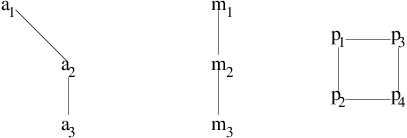
Indeed, we now claim that

\mathfrak{h}(a_{i}\times m_{j}\times p_{k})=\mathfrak{h}(b_{i}\times n_{j}\times p_{k})

for all $i=1,...,3$ , $j=1,...,3$ , and $k=1,...,4$ . This is exhibited, for example, by the obvious “large hexagon” containing the point at infinity in Figure 17, thought of as a Whitney disk from $a_{1}\times m_{1}\times p_{1}$ to $b_{1}\times n_{1}\times q_{1}$ (which is, of course, disjoint from $\mathbf{w}$ and $\mathbf{z}$ .

Thus, the ranks of the non-zero chain groups in each (relative) $\mathbb{Z}^{2}$ -grading are as illustrated in Figure 22.

We claim that in the filtration level given by $(1,-2)$ , the two generators $a_{3}\times m_{3}\times p_{4}$ and $b_{3}\times n_{3}\times q_{4}$ both survive in homology. This is true because the Maslov grading of $a_{3}\times m_{3}\times p_{4}$ is one greater than that of $b_{3}\times n_{3}\times q_{4}$ , and there are no positive domains from the first generator to the second. This can be seen at once by considering the domain connecting them illustrated in Figure 20. This is a domain from More specifically, that domain gives a domain $\phi\in\pi_{2}(b_{3}\times n_{3}\times q_{4},a_{3}\times m_{3}\times p_{4})$ with no negative local multiplicities (and Maslov index $-1$ ). From this, it is easy to see that there are no nowhere negative domains which miss all basepoints and have with Maslov index one between the two generators, and hence no differentials.

We claim also that in the filtration level given by $(-1,0)$ , the two generators $a_{1}\times m_{3}\times p_{2}$ and $b_{1}\times n_{3}\times q_{2}$ survive in homology. This is slightly more subtle, since there now is a (unique) domain connecting $a_{1}\times m_{3}\times p_{2}$ to $b_{1}\times n_{3}\times q_{2}$ , which has only non-negative local multiplicities (and Maslov index one). This domain is pictured in Figure 21. Perform an isotopy of the diagram, the “finger move” indicated by the dotted line in the figure, which introduces two new intersection points $t_{1}$ and $t_{2}$ of $\alpha_{1}$ with $\alpha_{2}$ . After this isotopy, all domains connecting the two fixed generators have both positive and negative multiplicities. It is important to note, though, that the isotopy introduces $18$ new generators, of the form $t_{i}\times a_{j}\times b_{k}$ $i\in\{1,2\}$ , $j,k\in\{1,2,3\}$ . However, using the small rectangle supported in the finger connecting $a_{1}\times t_{1}$ to $n_{3}\times q_{2}$ (which crosses no basepoints), we see that $t_{i}\times a_{1}\times a_{2}$ is in the same bigrading as $b_{1}\times n_{3}\times q_{2}$ , and hence that none of the newly-introduced intersection points is supported in $\mathbb{H}$ -grading $(-1,0)$ .

With this input, together with the usual symmetry property (Equation (4)), the link Floer homology polytope is determined immediately. In particular, it follows that the relative filtration levels displayed in Figure 22 indeed coincide with the absolute $\mathbb{H}$ -grading, and hence also that the homology groups in $\mathbb{H}$ -grading $(-1,3)$ , $(0,3)$ , $(1,2)$ , and $(1,1)$ are in fact trivial.

We conclude from this, together with Theorem 1.1 that the dual Thurston polytope for the Kinoshita-Terasaka link is as pictured in Figure 23. In particular, this suggests that the homology class dual to $(1,-2)$ is represented by a surface $F$ with $\chi(F)=-1$ . It is now an exercise in visualization to find such a representative (given by a sphere with three punctures).

Again, a more involved calculation using the same circle of ideas can be used to calculate the full link Floer homology groups of the Kinoshita-Terasaka link, given in Figure 24.

References

[1] R. Crowell. Genus of alternating link types. Ann. of Math. (2), 69:258–275, 1959.
[2] S. K. Donaldson. Lefschetz pencils on symplectic manifolds. J. Differential Geom., 53(2):205–236, 1999.
[3] D. Eisenbud and W. Neumann. Three-dimensional link theory and invariants of plane curve singularities, volume 110 of Ann. of Math. Studies. Princeton University Press, Princeton, NJ, 1985.
[4] Y. Eliashberg. A few remarks about symplectic filling. Geom. Topol., 8:277–293, 2004.
[5] Y. Eliashberg and W. P. Thurston. Confoliations, volume 13 of University Lecture Series. AMS, Providence, RI, 1998.
[6] J. B. Etnyre. On symplectic fillings. Algebr. Geom. Topol., 4:73–80, 2004.
[7] A. Floer. Morse theory for Lagrangian intersections. J. Differential Geometry, 28:513–547, 1988.
[8] A. Floer. The unregularized gradient flow of the symplectic action. Comm. Pure Appl. Math., 41(6):775–813, 1988.
[9] D. Gabai. Foliations and the topology of $3$ -manifolds. J. Differential Geom., 18(3):445–503, 1983.
[10] D. Gabai. Foliations and the topology of $3$ -manifolds III. J. Differential Geom., 26(3):479–536, 1987.
[11] M. Hedden. On knot Floer homology and cabling. Alg. Geom. Topol., 5:1197–1222, 2005.
[12] P. B. Kronheimer and T. S. Mrowka. Floer homology for Seiberg-Witten Monopoles. Preprint.
[13] P. B. Kronheimer and T. S. Mrowka. Scalar curvature and the Thurston norm. Math. Res. Lett., (4):931–937, 1997.
[14] P. B. Kronheimer, T. S. Mrowka, P. S. Ozsváth, and Z. Szabó. Monopoles and lens space surgeries. math.GT/0310164, to appear in Ann. of Math.
[15] C. T. McMullen. The Alexander polynomial of a $3$ -manifold and the Thurston norm on cohomology. Ann. Sci. de l’Ecole Norm. Sup., 35(2):153–171, 2002.
[16] K. Murasugi. On the Alexander polynomial of alternating algebraic knots. J. Austral. Math. Soc. Ser. A, 39(3):317–333, 1985.
[17] Y. Ni. A note on knot Floer homology of links. Geom. Topol., 10:695–713, 2006.
[18] Y. Ni. Sutured Heegaard diagrams for knots. Algebr. Geom. Topol., 6:513–537, 2006.
[19] P. S. Ozsváth and Z. Szabó. Heegaard Floer homology and alternating knots. Geom. Topol., 7:225–254, 2003.
[20] P. S. Ozsváth and Z. Szabó. Heegaard diagrams and holomorphic disks. In Different faces of geometry, Int. Math. Ser. (N. Y.), pages 301–348. Kluwer/Plenum, New York, 2004.
[21] P. S. Ozsváth and Z. Szabó. Holomorphic disks and genus bounds. Geom. Topol., 8:311–334, 2004.
[22] P. S. Ozsváth and Z. Szabó. Holomorphic disks and knot invariants. Adv. Math., 186(1):58–116, 2004.
[23] P. S. Ozsváth and Z. Szabó. Holomorphic disks and topological invariants for closed three-manifolds. Ann. of Math. (2), 159(3):1027–1158, 2004.
[24] P. S. Ozsváth and Z. Szabó. Heegaard Floer homology and contact structures. Duke Math. J., 129(1):39–61, 2005.
[25] P. S. Ozsváth and Z. Szabó. Holomorphic disks, link invariants, and the multi-variable Alexander polynomial. math.GT/0512286, 2005.
[26] J. A. Rasmussen. Floer homology and knot complements. PhD thesis, Harvard University, 2003.
[27] D. Rolfsen. Knots and links, volume 7 of Mathematics Lecture Series. Publish or Perish Inc., Houston, TX, 1990. Corrected reprint of the 1976 original.
[28] W. P. Thurston. A norm for the homology of $3$ -manifolds, volume 59 of Mem. Amer. Math. Soc., pages i–vi and 99–130. 1986.
[29] V. Turaev. Torsions of 3-manifolds, volume 4 of Geom. Topol. Monogr. Geom. Topol. Publ., Coventry, 2002.