Bruhat intervals as rooks on skew Ferrers boards
Abstract.
We characterise the permutations such that the elements in the closed lower Bruhat interval of the symmetric group correspond to non-taking rook configurations on a skew Ferrers board. It turns out that these are exactly the permutations such that corresponds to a flag manifold defined by inclusions, studied by Gasharov and Reiner.
Our characterisation connects the Poincaré polynomials (rank-generating function) of Bruhat intervals with -rook polynomials, and we are able to compute the Poincaré polynomial of some particularly interesting intervals in the finite Weyl groups and . The expressions involve -Stirling numbers of the second kind.
As a by-product of our method, we present a new Stirling number identity connected to both Bruhat intervals and the poly-Bernoulli numbers defined by Kaneko.
Key words and phrases:
Coxeter group; Weyl group; Bruhat order; Poincaré polynomial; rook polynomial; partition variety1991 Mathematics Subject Classification
Primary: 05A15; Secondary: 06A07, 14M151. Introduction
Since its introduction in the 1930s the Bruhat order on Coxeter groups has attracted mathematicians from many areas. Geometrically it describes the containment ordering of Schubert varieties in flag manifolds and other homogeneous spaces. Algebraically it is intimately related to the representation theory of Lie groups. Combinatorially the Bruhat order is essentially the subword order on reduced words in the alphabet of generators of a Coxeter group.
The interval structure of the Bruhat order is geometrically very important and has been studied a lot in the literature. From a combinatorial point of view, as soon as there is a (graded) poset, the following three questions naturally arise about its intervals (and they will probably arise in the following order):
- (1)
What is the rank-generating function (or Poincaré polynomial) ?
- (2)
What is the Möbius function ?
- (3)
What can be said about the topology of the order complex of ?
The third question was answered by Björner and Wachs [3] in 1982: The order complex of an open interval is homeomorphic to the sphere . The second question was answered already by Verma [18] in 1971: . However, the first question is still a very open problem!
For the whole poset was computed by Steinberg [17], Chevalley [5], and Solomon [16]. Really small intervals (of length in and in and ) were completely classified by Hultman [11] and Incitti [12]. Lower intervals of 312-avoiding permutations in were classified by Develin [6] (though he did not compute their Poincaré polynomials), and for a general lower interval in a crystallographic Coxeter group, Björner and Ekedahl [2] showed that the coefficients of are partly increasing. Apart from this, virtually nothing is known, not even for lower intervals.
The aim of this paper is to start filling the hole and at least gain some understanding of the rank-generating function of a family of intervals in finite Weyl groups. To this end we present a connection between the Poincaré polynomial and rook polynomials, making it possible to compute for various interesting intervals. Our approach is partly a generalisation of the notion of partition varieties introduced by Ding [7] to what may be called skew partition varieties.
The paper is composed as follows. In Section 2 we give a short introduction to rook polynomials before presenting our results in Section 3. In Section 4 we present the connection between rook polynomials and Poincaré polynomials and prove our main theorem. In sections 5 and 6 we apply our main theorem to intervals in the symmetric group . As a by-product a new Stirling number identity pops up at the end of Section 6. In Section 7 we apply our main theorem to the hyperoctahedral group . Finally, in Section 8 we discuss further research directions and suggest some open problems.
2. Rook polynomials
Let be a zero-one matrix and put rooks on some of the one-entries of . If no two rooks are in the same row or column we have a (non-taking) rook configuration on , and we say that covers the rook configuration. In the literature, is sometimes called a board and is often depicted by square diagrams like those in Figure 1. For convenience we will simultaneously think of as the set of its one-entries, and write for instance if and use notation like .
Let and denote reflecting the matrix upside down respectively rotating it 180 degrees, i.e. and if is an matrix. Define and similarly for rook configurations .
The number of rook configurations on with rooks is called the th rook number of and is denoted by . Given a nonnegative integer , following Goldman et al. [10] we define the th rook polynomial of as
Note that .
A zero-one matrix is a left-aligned (resp. right-aligned) Ferrers matrix if every one-entry has one-entries directly to the left (resp. to the right) and above it (provided these entries exist). The number of ones in the th row (resp. column) of is denoted by (resp. ). Figure 1 shows an example.

From [10] we have the following theorem.
Theorem 2.1 (Goldman et al.).
Let be a right-aligned Ferrers matrix of size . Then
Given a rook configuration on A, define the statistics to be the number of (not necessarily positive) cells of with no rook weakly to the right in the same row or below in the same column. In the special case where is an matrix and has rooks, becomes the number of inversions of the permutation given by , where is the row index and is the column index.
Next, (almost) following Garsia and Remmel [8], we define the th -rook number of as
where the sum is over all rook configurations on with rooks. Given a nonnegative integer , the th -rook polynomial of is defined as
Here is the -analogue of . Observe that putting yields the ordinary rook numbers and polynomials.
Garsia and Remmel showed that Theorem 2.1 has a beautiful -analogue:
Theorem 2.2 (Garsia, Remmel).
Let be a left-aligned Ferrers matrix of size . Then
where is the number of zero-entries in .
Let .
Corollary 2.3.
For the square matrix with ones everywhere, the th -rook number is
Let denote the zero-one matrix with ones on and above the secondary diagonal, i.e. . In [8, p. 248] it is proved that
| (1) |
where is the -Stirling number defined by the recurrence
with the initial conditions and for or .
3. Results
A skew Ferrers matrix is the difference between a Ferrers matrix and an equally aligned componentwise smaller Ferrers matrix . If and are left-aligned, then is also said to be left-aligned, and if and are right-aligned, so is .
Let denote the symmetric group. For any zero-one matrix , let be the set of rook configurations on with rooks. We will identify such a rook configuration with a permutation so that if and only if there is a rook at the square , where is the row index and is the column index.
For a permutation , let the right (resp. left) hull (resp. ) of be the smallest right-aligned (resp. left-aligned) skew Ferrers matrix that covers . Figure 2 shows an example.

For the definition of Bruhat order and a general treatment of Coxeter groups from a combinatorialist’s viewpoint, we refer to Björner and Brenti [1].
Our main result is the following theorem and its corollary.
Theorem 3.1.
equals the lower Bruhat interval in if and only if avoids the patterns 4231, 35142, 42513, and 351624.
Remark 3.2.
The permutations in the theorem are exactly the ones such that the Schubert variety corresponding to the interval is defined by inclusions in the sense of Gasharov and Reiner [9] according to their Theorem 4.2.
Corollary 3.3.
Let and suppose and both avoid the patterns 4231, 35142, 42513, and 351624. Then the following holds.
- (1)
equals the Bruhat interval .
- (2)
The Poincaré polynomial of equals the -rook number .
- (3)
In particular, the number of elements in equals the ordinary rook number .
Proof.
Once we observe that and recall that flipping the rook configurations upside down is an antiautomorphism on the Bruhat order on , the corollary follows directly from Theorem 3.1. ∎
Remark 3.4.
If is 312-avoiding then is an ordinary Ferrers matrix and Corollary 3.3 overlaps with Theorem 33 in [7] by Ding. In this case Ding coined the name partition variety for the Schubert variety corresponding to the Bruhat interval in . Thus it would be logical to coin the name skew partition variety for a Schubert variety corresponding to an interval such that .
Figure 3 shows two examples of the corollary.
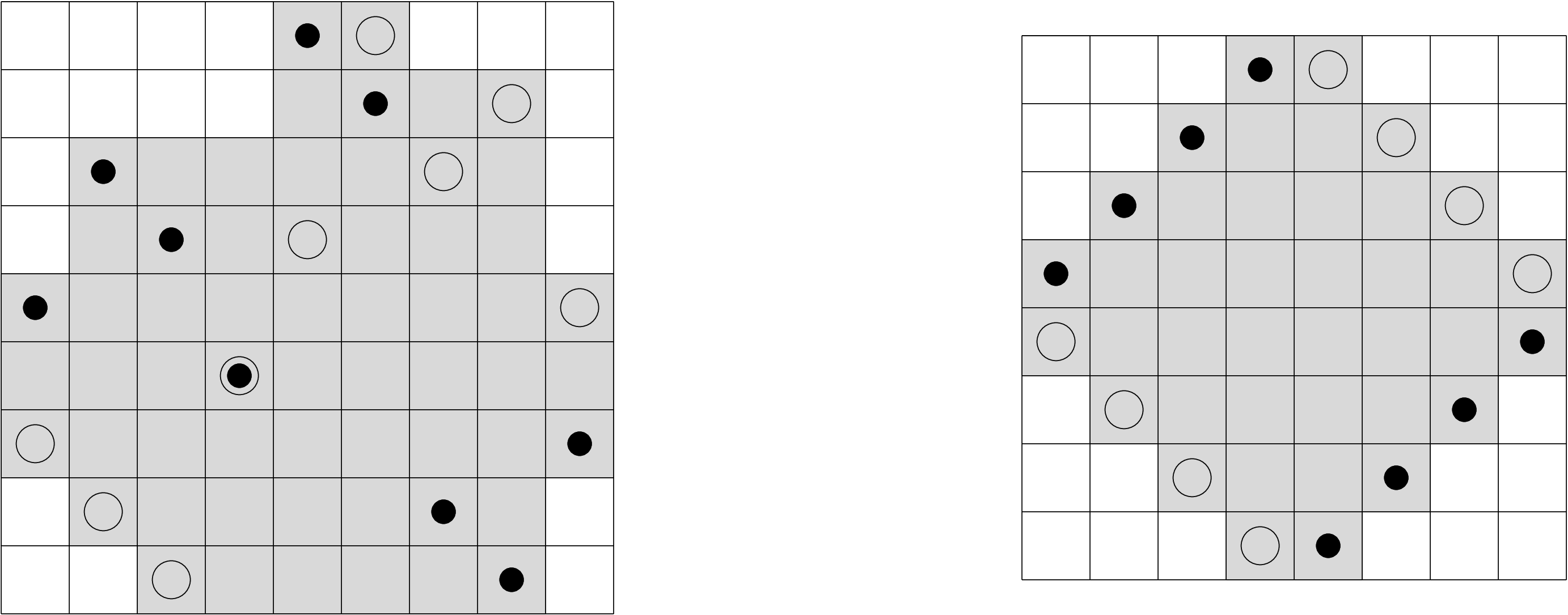
Nontrivial application of the above result yields the Poincaré polynomial of some particularly interesting intervals in finite Weyl groups.
For a Coxeter system and a subset of the generators, let denote the parabolic subgroup generated by . Each left coset has a unique representative of minimal length, see [1, Cor. 2.4.5]. The system of such minimal coset representatives is denoted by , and the Bruhat order on restricts to an order on .
We will deal with two infinite families of finite Coxeter systems, namely the symmetric groups and the hyperoctahedral groups . Their Coxeter graphs are depicted in Figure 4.
For type A we have the following result.
Theorem 3.5.
Let be the maximal element of . Then the Poincaré polynomial of the Bruhat interval is
The special case where is even, , and follows from Exercise 4.36 in Lovász [14] once one knows that the set of permutations he describes is a Bruhat interval (which is Exercise 2.6 in [1]). See also Theorem 3 in Vesztergombi [19].
For type B the corresponding result looks like this:
Theorem 3.6.
Let be the maximal element of . Then the Poincaré polynomial of the Bruhat interval is
We also present a recurrence relation for computing the number of elements in the Bruhat interval of where is any element in . As a by-product we obtain the following Stirling number identity which appears to be new.
Theorem 3.7.
Let be the maximal element of . Then the number of elements in the Bruhat interval is
where are the Stirling numbers of the second kind, and are the poly-Bernoulli numbers defined by Kaneko [13].
Remark 3.8.
Kaneko’s Theorem 2 says that for any . This is immediately evident from our new formula for the poly-Bernoulli numbers.
From Kaneko’s work [13, p. 223] we can compute the exponential bivariate generating function for .
The poly-Bernoulli numbers have the sequence number A099594 in Sloane’s On-Line Encyclopedia of Integer Sequences.
4. Skew Ferrers matrices and Poincaré polynomials
In this section we make a connection between Poincaré polynomials and rook polynomials, and prove Theorem 3.1.
Proposition 4.1.
If is a right-aligned skew Ferrers matrix of size , then is an order ideal in the Bruhat order of .
Proof.
The Bruhat order is the transitive closure of the Bruhat graph whose edges correspond to transpositions (see [1, Sec. 2.1]). Thus it suffices to show that we cannot leave by a transposition going down in the Bruhat order. In other words, if is a rook configuration on with rooks, and with , then exchanging rows and yields a rook configuration which is covered by . This is obviously true, as we can see in Figure 5.

∎
For and , let
In other words is the number of rooks weakly north-east of the square . The following criterion for comparing two permutations with respect to the Bruhat order is well-known (see e.g. [1, Th. 2.1.5]).
Lemma 4.2.
Let . Then if and only if for all .
Theorem 3.1 completely characterises the interesting cases where is a lower Bruhat interval . Now we are ready for the proof.
Proof of Theorem 3.1.
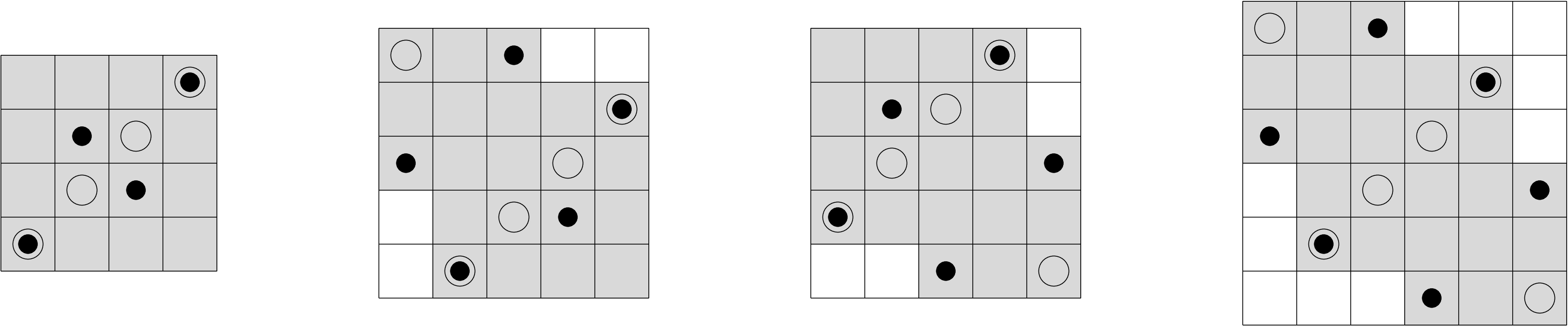
We begin with the “only if” direction which is the easier one. For each of the four forbidden patterns we will do the following: First we suppose contains the pattern. Then we move some of the rooks that constitute the pattern to new positions, and call the resulting rook configuration . This is seen to be covered by while in Bruhat order, and we conclude that is not uniquely maximal in .
Suppose contains the pattern 4231 so that there are rooks , , , and with and . Move the rooks and to the positions and and call the resulting rook configuration . Then is covered by and in Bruhat order so is not maximal in .
Note that the rooks outside the pattern turned out to be irrelevant for the discussion. In fact we could have supposed was equal to the pattern 4231 and then simply defined . This observation applies to the remaining three patterns as well, and thus the “only if” part of the proof can be written as a table that associates a to each pattern :
| 4231 | 4321 |
| 35142 | 15432 |
| 42513 | 43215 |
| 351624 | 154326 |
Figure 6 illustrates the table and makes it evident that is covered by in each case. That in Bruhat order can be checked easily using Lemma 4.2.
Now it is time to prove the difficult “if” direction. Suppose so that there is a with . Our goal is to show that contains some of the four forbidden patterns.
Let the rooks of and be black and white, respectively. (Observe that some squares may contain both a black and a white rook.) Order the squares partially so that if and , i.e. the north-east corner is the minimal square of .
Let be the set of squares with and no black rook weakly to the right of in row or above in column . First we show that is not empty.
Since , by Lemma 4.2 there is a square such that . Let be a minimal square with this property. Then there is no black rook weakly to the right of in row , for if that were the case the smaller square would have the property as well. Analogously, there is no black rook weakly above in column . Thus belongs to .
Now we can let be a maximal square in . Since we have and . There must be a black rook weakly to the right of in row because otherwise the greater square would belong to . By an analogous argument, there is a black rook weakly above in column . We have the situation depicted in Figure 7.
Since there are more white than black rooks inside the rectangle there must also be more white than black rooks inside the diagonally opposite rectangle . In particular there is at least one white rook inside and at least one white rook inside . Since is covered by it follows that there is a black rook inside and a black rook inside ; choose minimal in . Call and the witnesses. Now the situation is exactly as in the proof of Theorem 4.2 in [9] by Gasharov and Reiner. The remaining part of the proof will essentially be a copy of their arguments.
We show that at least one of the four forbidden patterns will appear, depending on whether the rectangle contains a black rook strictly to the left of column , and a black rook strictly below row . If one can find
- (1)
both, then combining these with the two witnesses produces the pattern 4231 in . (Look at Figure 8 for illustrations.)
- (2)
the former but not the latter, then combining the two witnesses with the former and with the black rooks in column and in row produces the pattern 42513.
- (3)
the latter but not the former, then combining the two witnesses with the latter and with the black rooks in column and in row produces the pattern 35142.
- (4)
neither, then combining the two witnesses with the black rooks in column and and in row and produces the pattern 351624.
∎
5. Poincaré polynomials of
In this section we apply Theorem 3.1 to the lower Bruhat interval of the symmetric group where is the maximal minimal coset representative . In the end we obtain the simple formula of Theorem 3.5.
Let denote the matrix with all entries equal to one. The following is a -analogue of the corollary to Theorem 1 in [4].
Proposition 5.1.
Let and be zero-one matrices of sizes and , respectively. The block matrix
has the th -rook number
Proof.
It is easy to see that each configuration of rooks on is chosen uniquely by the following procedure:
- •
First, choose a nonnegative integer .
- •
Then choose a configuration of rooks on and a configuration of rooks on . Together and form a configuration of rooks on .
- •
Let be the submatrix consisting of the remaining free one-entries of , i.e. the one-entries whose row and column have no rook in or . Similarly, let be the submatrix consisting of the remaining free one-entries of . Now choose a configuration of rooks on and a configuration of rooks on .
Let be the set of inversions of , i.e. pairs of rooks such that is strictly north-east of . The number counts the cells in which have no rooks to the right or below. This equals the number of inversions such that belongs to or and belongs to or :
Similarly, counts the cells in which have no rooks to the left or above, so
We also have
and
Putting the above equations together yields
| (2) | |||||
where . Now we exponentiate and sum over all permutations which can be constructed by the procedure above:
By Corollary 2.3, . ∎
6. The number of elements in a lower interval of
For a general minimal coset representative , it seems very hard to compute the complete Poincaré polynomial. In this section we will solve the easier problem to determine , i.e. the number of elements of . We obtain a recurrence relation that allows us to count the elements in polynomial time. In the special case when is the maximal element in this method results in a formula different from what we get if we put in Theorem 3.5. From this, rather unexpectedly, we obtain an identity of Stirling numbers that we have not seen in the literature.
The set of minimal coset representatives consists of the permutations with and . Such a permutation clearly avoids the patterns in Corollary 3.3 so the number of elements in the Bruhat interval is given by the th rook number . Fortunately has a simple structure. If then, as can be seen in Figure 9,
so the interval is isomorphic (as a poset) to the interval in , where for . Thus we may assume that . Then , where and are right-aligned Ferrers matrices with row lengths

For , let be the zero-one matrix with ones in the cells . It is easy to see that a rook configuration with rooks is covered by if and only if it is covered by and not by any . Thus, by the principle of inclusion-exclusion we get
By a suitable permutation of the rows, the matrix can be transformed to a Ferrers matrix with column lengths
where denotes the image of under . Theorem 2.1 with gives
As we will see in a moment, this expression can be computed efficiently by dynamic programming.
For and , let
where denotes the set of subsets of of size . Also put if . It is straightforward to verify the following recurrence relation:
| (3) |
Here is Dirac’s -function which is 1 if and 0 otherwise. Since
| (4) |
the number of elements in is computable in polynomial time.
A special application of the method above admits us to prove our by-product Theorem 3.7.
Proof of Theorem 3.7.
Consider the case when is the maximal element in , i.e. . Then if and if , so the recurrence (3) becomes
Iteration of the first line of the recurrence yields
| (5) |
Putting for , our recurrence transforms to
We recognise this as the recurrence for where are Stirling numbers of the second kind; thus for . Combining this with Equation (5) and plugging the result into Equation (4), we obtain
which also can be written as
This happens to be the formula for the poly-Bernoulli number defined by Kaneko [13]. ∎
7. Type B
In this section we compute the Poincaré polynomial of the lower Bruhat interval in the hyperoctahedral group , where is the maximal minimal coset representative, .
We will represent combinatorially by the set of rotationally symmetric maximal rook configurations on , see [1, Ch. 8]. In this representation in Bruhat order on if and only if as elements of ([1, Cor. 8.1.9]). The rank of is
| (6) |
where is the usual inversion number of as an element of , and , see [1, Ch. 8, Exercise 2].
For a zero-one matrix of size , let
Proposition 7.1.
Let be a zero-one matrix of size . Then
Proof.
The proof is almost identical to the proof of Proposition 5.1.
When , it is easy to see that the permutation constructed by the procedure in the proof of Proposition 5.1 is rotationally symmetric if and only if and . Thus, putting , , , , and into Equation (2) and using the identity , we obtain
Obviously, . Exponentiation and summation over all rotationally symmetric permutations on yields
By Corollary 2.3 . ∎
Now we are ready for the proof of Theorem 3.6.
8. Open problems
Perhaps the reason we still do not know much about the Poincaré polynomials of Bruhat intervals after several decades of research in the area is the lack of natural methods to attack it. We hope the framework and the tools presented here will make the problem more accessible, and we would like to suggest a number of interesting open questions.
- •
What is the Poincaré polynomial in the even-signed permutation group if is the maximal minimal representative in the quotient modulo a maximal parabolic subgroup isomorphic to ?
- •
What is in the affine group ?
- •
Are there formulas for the generalized Eulerian polynomial or even for the bivariate generating function , where is the descent number of ?
- •
In a recent paper by Björner and Ekedahl [2] it is shown (for any crystallographic Coxeter group) that implies , where is the -coefficient of . Perhaps one can say more about the particular Poincaré polynomials discussed in the present paper. Are they unimodal, for instance?
- •
As noted by Gasharov and Reiner [9, p. 559], Ding’s partition varieties [7] correspond not only to certain Bruhat intervals of the whole group but also to some intervals of the quotient for certain parabolic subgroups . Can something similar be done in the more general setting of skew partition varieties?
- •
Given a polynomial, what board (i.e. zero-one matrix), if any, has it as its rook polynomial? In a recent paper [15] Mitchell showed that distinct increasing Ferrers boards have distinct rook polynomials. What is true for skew Ferrers boards?
- •
9. Acknowledgement
I would like to thank Torsten Ekedahl for asking a question that made me write this paper. Many thanks also to Anders Björner for introducing me to Coxeter groups and Schubert varieties.
References
- [1] A. Björner and F. Brenti. Combinatorics of Coxeter Groups. Springer, 2005.
- [2] A. Björner and T. Ekedahl. On the shape of Bruhat intervals, arXiv:math.CO/0508022.
- [3] A. Björner and M. Wachs. Bruhat order of Coxeter groups and shellability. Adv. in Math., 43:87–100, 1982.
- [4] G.-S. Cheon, S.-G. Hwang, and S.-Z. Song. Rook polynomials to and from permanents. Discrete Math., 264:25–36, 2003.
- [5] C. Chevalley. Sur certain groupes simples. Tôhoku Math. J., 7:14–66, 1955.
- [6] M. Develin. Rook poset equivalence of Ferrers boards. AIM 2005-1, arXiv:math.CO/0502107.
- [7] K. Ding. Rook placements and cellular decomposition of partition varieties. Discrete Math., 170:107–151, 1997.
- [8] A. M. Garsia and J. B. Remmel. Q-counting rook configurations and a formula of Frobenius. J. Combin. Theory Ser. A, 41:246–275, 1986.
- [9] V. Gasharov and V. Reiner. Cohomology of smooth Schubert varieties in partial flag manifolds. J. London Math. Soc., 66(2):550–562, 2002.
- [10] J. Goldman, J. T. Joichi, and D. White. Rook theory I. Rook equivalence of Ferrers boards. Proc. Amer. Math. Soc., 52:485–492, 1975.
- [11] A. Hultman. Bruhat intervals of length 4 in Weyl groups. J. Combin. Theory Ser. A, 102:163–178, 2003.
- [12] F. Incitti. New results on the combinatorial invariance of Kazhdan-Lusztig polynomials. preprint, 2005.
- [13] M. Kaneko. Poly-Bernoulli numbers. J. Théor. Nombres Bordeaux, 9:221–228, 1997.
- [14] L. Lovász. Combinatorial Problems and Exercises. Elsevier Science Publishers and Akadémiai Kiadó, 2nd edition, 1993.
- [15] A. G. Mitchell. The inverse rook problem on Ferrers boards, arXiv:math.CO/0407007.
- [16] L. Solomon. The orders of the finite Chevalley groups. J. Algebra, 3:376–393, 1966.
- [17] R. Steinberg. Endomorphisms of linear algebraic groups. Mem. Amer. Math. Soc., 80:1–108, 1968.
- [18] D.-N. Verma. Möbius inversion for the Bruhat order on a Weyl group. Ann. Sci. École Norm. Sup., 4:393–398, 1971.
- [19] K. Vesztergombi. Permutations with restriction of middle strength. Studia Sci. Math. Hungar, 9:181–185, 1974.