Categorified Algebra and Quantum Mechanics
Abstract.
Interest in combinatorial interpretations of mathematical entities stems from the convenience of the concrete models they provide. Finding a bijective proof of a seemingly obscure identity can reveal unsuspected significance to it. Finding a combinatorial model for some mathematical entity is a particular instance of the process called “categorification”. Examples include the interpretation of as the Burnside rig of the category of finite sets with product and coproduct, and the interpretation of as the category of combinatorial species. This has interesting applications to quantum mechanics, and in particular the quantum harmonic oscillator, via Joyal’s “species”, a new generalization called “stuff types”, and operators between these, which can be represented as rudimentary Feynman diagrams for the oscillator. In quantum mechanics, we want to represent states in an algebra over the complex numbers, and also want our Feynman diagrams to carry more structure than these “stuff operators” can do, and these turn out to be closely related. We will show how to construct a combinatorial model for the quantum harmonic oscillator in which the group of phases, , plays a special role. We describe a general notion of “-Stuff Types” for any monoid , and see that the case provides an interpretation of time evolution in the combinatorial setting, as well as other quantum mechanical features of the harmonic oscillator.
1. Introduction
One reason for the success of category theory has been its ability to describe relations between seemingly separate areas of mathematics. Here, we will describe how category theory can be used to see relationships between enumerative combinatorics and quantum mechanics. Specifically, we examine an approach to understanding the quantum harmonic oscillator by “categorifying” the Fock representation of the Weyl algebra - which is the algebra of operators on states of the oscillator. This builds on work described by Baez and Dolan[1]. Since we do not expect readers to be expert in both quantum mechanics and category theory, we have tried to make this paper as self-contained as possible. Many definitions and explanations will be well-known to the experts in each field, and are arranged by section as much as possible to allow readers to skip familiar material.
Categorification is best understood as the reverse of “decategorification”. This is a process which begins with some category, and produces a structure for which isomorphisms in the original category appear as equations between objects instead. Categorification is the reverse process, replacing equations in some mathematical setting with isomorphisms in some category in a consistent - but possibly non-unique - way. One example is the way we can treat the category of finite sets as a categorification of the natural numbers . The set can be seen as a set of cardinalities indexing isomorphism classes of finite sets, and which get their addition and multiplication from the categorical coproduct and product on the category of finite sets. We will see further examples of a connection between decategorification and cardinality.
Joyal [12] has described the category of structure types, which can be seen as the categorification of a certain ring of power series. These structure types play an important role in enumerative combinatorics, in which “generating functions” of given types of structures can be used in a purely algebraic way to count the number of such structures of various sizes. These generating functions are “decategorified” versions of structure types - or, equivalently, cardinalities of them. In section 2, we describe how this works in more detail, and give some examples.
This leads, in section 3, to the application to quantum mechanics. In that section, we describe briefly the quantum harmonic oscillator. It has a Hilbert space of states, and the Weyl algebra is the algebra of operators on this space. The Weyl algebra has a representation as operators on Fock space - the space of formal power series in one variable with a certain inner product. Here, it is generated by two operators - the creation and annihilation operators. We show how this algebra can be categorified using the category of structure types as a replacement for Fock space, and a certain class of functors as the operators.
In section 4, we find that structure types do not have a rich enough structure to capture all properties of power series. In particular, they do not provide a natural way to treat power series as functions which can be evaluated or composed in a way which is compatible with the idea of cardinality for structure types. To properly categorify these ideas, one can extend the notion of structure type to a so-called “stuff type”. This makes use of the fact that there are two ways of seeing structure types as functors. One is as a functor taking each finite set to the set of structures of a certain type which can be placed on them - the functor gives “coefficients” associated to finite sets. The other point of view treats structure types as “bundles” over the category of finite sets, whose projections take structured sets to their underlying sets. The latter point of view allows a larger class of “total spaces” for the bundle - in fact, it can be any groupoid. We describe a classification of functors, and show how dropping the requirement of faithfulness on the projection functor for the bundle leads to stuff types. In appendix B we provide more details, showing how stuff types form a category of “groupoids over finite sets”.
Section 5 examines operations on stuff types which are useful to the program of categorifying quantum mechanics. The category of stuff types naturally gets an “inner product” on objects by means of a pullback construction. We then show this is a categorification of the usual inner product on Fock space. Then we describe the equivalent of linear operators on Fock space - “stuff operators”, and show how they can be seen directly as categorified matrices. These can act on stuff types by a construction similar to the inner product, as one might expect. We then develop some particular examples of stuff operators, namely the equvalent of the creation and annihilation operators. These provide a connection to Feynman diagrams.
Then, in 6, we introduce the idea of -sets, labelled with elements of a general monoid , extend this from sets to general groupoids, and describe an idea of cardinality for these. Of special interest for quantum mechanics is the group , the group of phases. We see that it is possible, by “colouring” sets (interpreted as sets of quanta) with these phases, to recover more features of the quantum harmonic oscillator. In particular, we describe an -stuff operator which corresponds to time evolution of a state without interactions. We also demonstrate a connection between stuff operators and Feynman diagrams.
Finally, we summarize the results, and suggest directions in which this work could be extended.
2. Structure Types
2.1. Categorification of and
Before we can study structure types, we need to see how a category with products and coproducts gives rise to a rig, which is to say an object like a ring, possibly without negatives (see Appendix A for a more precise definition). A simple example is the free rig on no generators - that is, (generated by the nonzero element under addition, this has no extra generators or relations, so it has a natural homomorphism into any rig). Natural numbers are called by this name because they arise naturally as counting numbers - namely, numbers we use to give the cardinality of some finite set of things. Bijections between finite sets are what make counting possible (for example, bijections of fingers and sheep), so these cardinalities are actually equivalence classes of finite sets under an equivalence relation given by bijections.
This suggests looking the category of finite sets, with a cardinality map given by taking sets to their isomorphism classes. The cardinality map turns this category into a rig. Since its decategorification is a rig, we say this category is an example of a 2-rig - a category with a monoidal operation like multiplication, and a coproduct structure giving addition (for a more precise definition, see Appendix A). The cartesian product of sets gives the multiplication in , and disjoint union gives addition. An analogous process makes sense for any 2-rig, but a reverse process, starting with any rig, is more difficult.
For a more involved example, consider the problem of categorifying the free rig on one generator, (the rig of polynomials in with natural number coefficients). We can think of this as a rig of functions from to in at least two different ways. One treats an element as the map taking to the natural number . The second takes to the coefficient of the power of in , denoted . It is interesting to compare how multiplication of these formal power series is represented in each representation. In the first case, we have pointwise multiplication:
In the other, mulitplication looks like convolution:
| (1) |
We’ll return to the first way of looking at them later when we study “stuff types”. The second representation will be better for now, because it treats power series as purely formal, rather as functions. To categorify the rig seen as the rig of functions , we naturally expect to look at a corresponding 2-rig of functors (see appendix A for more on 2-rigs):
Definition 1.
A structure type is a functor from the category whose objects are finite sets, and whose morphisms are the bijections11 1 is Joyal’s (for “bijection”). It makes no difference from which universe we take these sets - a skeletal version of consisting of only pure sets, one per cardinality, will do as well as any other for our purposes., into the category :
These functors naturally form a category whose morphisms are the natural transformations . We denote this category by .
We say that image of a set is the set of all “structures of type ” which can be placed on . Now recall that structure types can be seen as categorified formal power series. The “coefficients” are in the category of sets and maps than the groupoid of finite sets and bijections (though, since all maps in are bijections, so are their images). Since we allow the possibility of infinite sets as coefficients, these are more general than power series. There is no loss in adopting this approach, except when it comes to taking cardinalities - an issue we will consider when we discuss stuff types (in section 4.2.1).
An example of a structure type is the type of “graphs on finite sets of vertices”. So then the image of a given finite set is just the set of all such graphs on . The morphisms in , give , which are maps of the structures (graphs) on to those on . These maps are compatible with the given bijection of underlying elements: they amount to consistent relabellings of all the vertices in all the graphs according to the bijection . In particular, permutations of give automorphisms of .
To take the cardinality of a structure type, let be the set of -structures on the finite set (we will elide the difference of notation between a set and its cardinality). Then the cardinality of the structure type is the formal power series
| (2) |
where is just the usual set cardinality of . We will see later how this formula for the cardinality is a manifestation of “groupoid cardinality”, but note for now that the formula for given above is known as the “generating function” for -structures. This is a well known and useful idea in combinatorics (and generalizes considerably beyond this example - see, e.g. [16] and [3] for more on the whole subject).
Example 1.
The simplest example is for the type , which we call “being a one-element set”. This structure can be put on a one-element set in just one way, and in no ways on any other. The set of all -structures on contains just itself if has exactly one element, and is empty otherwise. The cardinality of the type is easily seen to be just .
Similarly, we have the type “being an -element set”, denoted by , since it has cardinality .
Generating functions (cardinalities of structure types) can be used to find cardinalities of types defined in terms of simpler types. We make this more precise with the following definition and theorem:
Definition 2.
Given two structure types and , there are sum and product structure types and , defined as follows. Putting an -structure on a set consists of making a choice of or , and putting a structure of that type on . Putting an -structure on consists of splitting into an ordered pair of disjoint subsets, then putting an -structure on the first part and a -structure on the second part.
Conceptually, we associate addition with “or” (an -structure or a -structure), and we associate multiplication with “and” (a splitting into an -structure and a -structure). This is similar to the categorified notions of addition and multiplication for as disjoint unions and cartesian products in . This reappears when we look at functors from to , and allows us to categorify the algebraic operations on the rig as well.
Theorem 1.
If and are two structure types, then and
Proof.
To see that , just note that the set of -structures on the set consists of the disjoint union of the set of -structures and the set of -structures, since by definition such a structure consists of a choice of or together with a structure of the chosen type. Thus, the set cardinalities satisfy , from which the result follows from the definition by linearity.
Now, as for , we have that
| (3) | |||||
This follows directly from the fact that the number of -structures on an -element set is a sum over all from to of a choice of a -element subset of , multiplied by the number of -structures on the chosen -element subset and of -structures on the remaining -element set. ∎
These facts suffice to prove that the functor category is a 2-rig (in fact, it is the free 2-rig on one generator),
Theorem 2.
The category is a 2-rig whose monoidal operation is the product defined above.
Proof.
See Appendix A. ∎
The 2-rig structure of lets us find useful information about types of structure defined in terms of simpler types using the sum and product operations we have defined, such as many recursively-defined structures. In particular, it makes sense of many calculations done with generating functions in combinatorics. A simple example shows that the factor of in the cardinality formula is due to the fact that we do not think of the set as ordered.
Example 2.
Define the type using the product operation in terms of the type , “being a one-element set”. In particular, we say , and recursively define . Then by theorem 1, we have . Now we observe that we can interpret as the type of “total orderings on an -element set”. Since a structure in the product involves a choice of two distinguishable subsets, we can find a unique total ordering on the set by assuming one to precede the other, and defining the total order recursively. So in fact a structure can be seen as just a total order. And, indeed, there are total orderings, so the type of the cardinality is .
Now note that the structure “being a finite set” is the sum over all of the types “being an -element set”: . Since each coefficient is 1, the cardinality of this type is , so we denote the type by .
If is the structure “being a totally ordered set” (that is, an structure on is a total ordering on ), then so that:
| (4) |
In [3], it is shown that many tree-like structures can be defined using the operations on structure types we have described. Binary trees provide an elementary example.
Example 3.
An example of a structure-type is the type Binary trees, which we denote . To put a -structure on a finite set is to make into the set of leaves of a binary tree. This is a recursively-defined tree structure, which is either a bare node (leaf), or a node with two branches, where each branch is another binary tree. That is:
since the structure type is the type ”being a one-element set” (a leaf), and is the type which, put on some set of elements, divides them into two subsets and puts a -structure on each one. Some typical binary trees are shown in figure 1
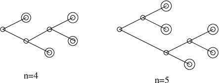
This highlights the close relationship between structure types and power series, since solving this recursive formula directly (for instance, by repeated substitution of the definition of into the term in the definition (or by solving the quadratic equation for !) shows that is isomorphic to a structure type which we can write as the analog of a power series, beginning:
where the coefficients are the Catalan numbers. This enumerates binary trees of each size: is equivalent to a direct sum over all sizes of sets of some number of copies of the structure “being an -element set”. Specifically, this number is times the Catalan number: the number of labellings of the leaves of an -leaf binary tree by the elements of some given -element set .
3. Structure Types and the Harmonic Oscillator
We have defined structure types as functors of a certain kind (faithful functors ), and made the analogy between these and formal power series. Just as a single formal power series is really only of interest in the setting of the space of all formal power series, so too a given structure type acquires more meaning when we think of it in the setting of all such functors. In particular, one thing we are interested in for the purposes of categorifying quantum mechanics are the categorified versions of algebras of operators on this space.
To see why this is so, we will first describe the Weyl algebra - an algebra of operators on the Hilbert space of states of the quantum harmonic oscillator - then see how to use structure types to categorify it. Readers who are familiar with quantum mechanics may wish to skip to section 3.2
3.1. The Quantum Harmonic Oscillator
3.1.1. The Weyl Algebra and its Representations
States of the quantum harmonic oscillator can be represented as formal power series with coefficients in , where the state corresponds to the pure state with energy , and a power series represents a superposition (linear combination) of these pure states with given complex amplitudes. We will study the harmonic oscillator using the Weyl algebra, which consists of operators on the space of states, and is generated by two operators satisfying certain commutation relations. There are two important representations the Weyl algebra, which are easy to describe in terms of generators. These are the Fock and Schrödinger representations.
Definition 3.
The Weyl algebra is the complex algebra generated by the ladder operators, namely the creation operator and the annihilation operator . These satisfy the relations . The Fock representation of the Weyl algebra on the vector space of formal power series in is determined by the effect of these generators:
| (5) |
and
| (6) |
In other words, , the derivative operator, and , the operator “multiplication by ”. It should be clear that these satisfy the defining commutation relations, since . These operators do not correspond to quantum-mechanical observables (which must be self-adjoint); instead, these are operators which add or remove a quantum of energy to a state.
We can build many operators from just and . One which often appears is the operator
| (7) |
called the “field operator”, which produces a superposition of the states in which the system has lost one quantum or gained one quantum of energy (in some interaction).
Another important operator is the number operator, denoted , which is just
| (8) |
This is related to the energy of the system - which is the Hamiltonian for the evolution of the oscillator. It should be clear that the eigenvalues of are just the natural numbers , and an eigenstate corresponding to the eigenvalue is the state (a pure state with energy ). These ladder operators give us the key to seeing the Weyl algebra in the categorified setting, when we pass from formal power series to structure types.
The other representation mentioned was the Schrödinger representation. Here we think of the Weyl algebra as generated by a different pair of generators:
Definition 4.
Two generators and of the Weyl algebra are given in terms of and by
| (9) |
or equivalently,
| (10) |
Physically, is the momentum operator, whose eigenstates are pure states with definite momenta which are the eigenvalues of , and is the position operator, whose eigenstates have position given by the corresponding eigenvalues. We can take these as the defining generators of the Weyl algebra, since these generate everything in it (given either pair of generators, the other is uniquely defined). Moreover, they satisfy the relations:
| (11) |
We could have taken this as the definition of the Weyl algebra, instead.
Definition 5.
A Schrödinger representation of the Weyl algebra is a representation on a space of functions , with the position operator and momentum operator represented as
| (12) |
The space of functions on which the and operators act is commonly taken to be the Schwartz functions. These are smooth functions all of whose derivatives (including the functions themselves) decay to zero faster than the reciprocal of any polynomial (so in particular they are functions).
We can note that these and satisfy the commutation relations above, by exactly the same argument as used for the ladder operators in the Fock representation. It is interesting, but potentially confusing, that in both representations the generators can be represented as multiplication and differentiation. In fact, every representation of the Weyl algebra has such a form, but the variables in which power series are expanded will have different interpretations. The variable of functions in the Schrödinger representation is literally the position variable for the oscillator, whereas in the Fock representation is simply a marker, whose exponent represents the energy of a state.
In fact, we will focus entirely on the Fock representation, and will see that it has a natural combinatorial interpretation, which we will describe in terms of the generators and , and involving structure types. We can think of this interpretation as a categorification of the Fock representation of the Weyl algebra. Developed further, it will show close connections to the theory of Feynman Diagrams, as we shall see in section 5.3.
3.1.2. The Inner Product on Fock Space
Now, we should remark here that in representing the quantum harmonic oscillator, like any quantum system, the two essential formal entities we need are a Hilbert space and an algebra of operators on this space, including self-adjoint operators corresponding to the physical observables of the system. We have described the Weyl algebra as its acts on the Hilbert space of power series, but we haven’t completely described this space, since to make it a Hilbert space, we need an inner product. Clearly, as a vector space, is spanned by , but there are many ways to put an inner product on this - and from each one, we get a Hilbert space from the subset consisting of the elements with finite norm. So we need to choose the physically significant inner product in order to specify the Hilbert space of states of the oscillator.
The inner product represents the complex amplitude, whose squared norm is a probability, for some combination of a state-preparation process and a measurement process (a “costate”). The inner product of two states is a “transition amplitude” the amplitude for finding a system set up in state to be in state on measurement. If the system undergoes a change of state between set-up and measurement, there will be an operator applied to one side. Self-adjoint operators correspond to observable quantities, whose eigenvalues are the possible values which can be observed.
For physical reasons, we say that the inner product of two states having different energy should be zero: . That is, the probability of setting up a state with energy and observing the state to have a different energy should be zero by conservation of energy, if there are no intermediate interactions.
Since position and momentum are observable quantities, we want the corresponding operators and we described along with the Schrödinger representation - to be self-adjoint. But then we must have : i.e. the ladder operators must be adjoints. A straightforward calculation then reveals:
| (13) |
Normalizing so that (here, the vector represents the vacuum, or ground, state, where there are no quanta of energy present), we get that the physically meaningful inner product on power series is the following:
Definition 6.
The inner product on is defined by its operation on the basis by . The space of states of the harmonic oscillator consists of all power series with finite norm according to this inner product.
The particular form of this inner product turns out to be closely involved with the connection between this quantum system and structure types, and in fact this inner product will turn out to have a natural categorification in the setting of “stuff types”, which we see in section 4.2.1.
A standard question one may ask about the quantum harmonic oscillator is to find an “expectation value” like , where. Recall that the field operator takes a state and gives a superposition of states in which it has gained and lost one quantum of energy. Thus, the expectation value may be nonzero, so long as is at least as large as the difference between and . This is the kind of value which can be calculated by means of Feynman diagrams.
What we mean to show now is that the categorified expectation value above has a direct interpretation in terms of a groupoid whose objects just look like Feynman diagrams. To see this, we first start with a description of a categorified Weyl algebra.
3.2. Structure Types and the Weyl Algebra
We have said already that structure types are a categorified version of formal power series (with natural number coefficients). We want to use them to help us categorify the Weyl algebra, which is generated by and in the algebra of operators on such series. To do this, we must develop operators on structure types (that is, natural transformations between functors) which correspond to these in the decategorified form.
This amounts to finding a combinatorial interpretation of the operators and , since a structure type is a combinatorial entity: it identifies a kind of structure which can be put on a finite set, and decategorifying it gives a “generating series” for those sorts of structures. The coefficients of this series count the number of such structures, which is the cardinality - and thus decategorification - of the set of such structures. The combinatorial flavour of structure types is made clearer, for example, when we can define them recursively, or otherwise show some relationships between the structures on different sets. These properties can sometimes be expressed as algebraic or differential equations involving the generating series.
A pure state with quanta of energy, in the representation of the Weyl algebra described above, corresponds to the state . The categorified version of this state, , in the structure-type setting, is the structure “being a finite set with elements” (that is, this is the structure which can be put in exactly one way on an element set and no ways on any other set). It seems natural to identify the elements of the sets on which we put our structures with quanta of energy of the quantum harmonic oscillator, and this is what we will do. A categorified state is a structure type - a type of structure which can be put on some set of quanta of energy, which we can express in the basis of the 2-Hilbert space of states (). It is characterized by the set of -structures on each size of finite set, and the ways those structures transform as we relabel the underlying set of quanta.
We want to define two operators on structure types, and , which correspond to differentiation with respect to and multiplication by in the Fock representation of the Weyl algebra. In fact, these are just the “insertion” and “removal” operators, familiar in combinatorics:
Definition 7.
The structure-type operator acts on a structure type to give a structure type , for which putting an -structure on a set is to adjoin a new element, which we denote , to and then put an -structure on . The adjoint operator, is the one which acts on a structure type by giving a structure type for which putting an -structure on a set is the same as removing an element from and putting an -structure on the resulting set.
It should be clear that acts like differentiation, by seeing how it acts on , since is the structure which, to put it on a set, means putting the structure of “being a totally ordered -element set” on . There are ways to do this, provided is an element set (one for each position might take in the total ordering), so is equivalent to putting the structure of “being a totally ordered -element set on and also choosing one of positions:
| (14) |
And in general, acts like differentiation on structure types (we can extend the above property linearly).
Now to see how acts, note that since an -structure on S is equivalent to a way of splitting S into two parts, putting an structure on one, and the structure of being a 1-element set on the other, we can see even more directly that acts as (categorified) multiplication by . The commutation relation now can be seen as a decategorification of the corresponding property of the operators and . To summarize:
Theorem 3.
The structure type operators and satisfy
| (15) |
and
| (16) |
and
| (17) |
To see these ideas more concretely, consider the following examples:
Example 4.
A categorified state is just a structure type. One such type is “being a finite set”, which we can denote ( from the French “ensemble”, but also appropriate in light of the generating series for this type). Then putting an -structure on a finite set is the same as putting an structure on , and there is exactly one way to put an -structure on ANY finite set, hence exactly one way to put an -structure on as well. That is, . This makes sense, since , and so this equation becomes when we take its cardinality.
Example 5.
Consider the structure type , “being a totally ordered finite set” (or “of total orderings on a finite set”). There are such structures on a finite set , so we can see this type as isomorphic to
| (18) |
(since is the type of totally ordered -element sets). Here, the sum is to be understood as a coproduct. Then to put an -structure on a set , one puts a total order on : this amounts to splitting into two (ordered) parts and putting a total order on each part. That is, an -structure is the same as an -structure, which is a combinatorial interpretation of the algebraic fact that . Extending this further, an -structure on consists of putting a total order on with two extra elements adjoined - thereby dividing into three parts (in order) and totally ordering these. There are two ways to build such a structure with - and -structures: to divide in two and put an -structure (equivalently, -structure) on the first part and an -structure on the second, or to do this in the reverse order. Thus, - a combinatorial interpretation of the fact that . This pattern continues for general .
This representation of the Weyl algebra in terms of these operators on structure types gives us a model in which the ladder operators have immediate meaning in terms of adding and removing elements to sets, and the states of the system are given as kinds of structures which can be put on those sets. The sets in question are sets of quanta of energy in the system. A categorified state consists of a type of structure which can be put on these quanta. The number of such structures for each number of quanta is related to the amplitude for the state to have that energy by means of the inner product on the Hilbert space given in equation 13. We shall see a combinatorial interpretation for this inner product in a later section, and see that it has a direct relationship to Feynman diagrams for energy quanta in the harmonic oscillator. This suggests what we must do next: we have recovered the basic structure of the Weyl algebra in a categorified form, but so far we are missing some concepts which, though quite natural in the decategorified setting, are difficult to see in this combinatorial picture. These are evaluation of power series at particular points, and the inner product of the Hilbert space (which will become a 2-Hilbert space in the categorified setting, once we have described the inner product). To describe these adequately, we shall examine a generalization of structure types, which we call “stuff types”.
4. Stuff Types
We have described a structure type as a functor , where the image of each finite set is the set of structures “of type ” which can be put on , but it should be obvious that the category is rather larger than we need, since for most sorts of structures we can think of, almost all sets will not appear in the image at all - most are not sets of structures on an -element set for any or . If we think of a category whose objects are precisely the structures of type , and whose morphisms are those maps which arise from bijections of the underlying sets, we have a category better suited to . This category is, in fact, a groupoid (i.e. a category in which all morphisms are iso), since is.
If we do this, however, we now have not sets of structures as objects, but -structures themselves, and there are many such structures corresponding to each . So now it is more natural to think of as a functor:
where each object of is taken to its underlying set, and each morphism to the underlying bijection of sets. So every morphism in the image, , then comes from morphisms in under this . A functor with this property is called faithful.
Why should we make this changed to the definition of a structure type? There are at least two good reasons to take this approach. One is that, while the previous definition fit well with the view of formal power series in which we are interested in finding the coefficient of the power of , this definition allows us to think of as corresponding to a power series which we evaluate at various (positive) real numbers to get other (positive) real numbers. To see how this works, we first remark that it will make sense to think of a structure type being evaluated at a groupoid, and so we need some useful facts about these.
4.1. Groupoids
To begin with, we recall what kind of category we are dealing with here:
Definition 8.
A groupoid is a category in which all morphisms are invertible.
A group is a special example of a groupoid, with only one object - then the elemnts of the group correspond to morphisms of the groupoid. Another special case of a groupoid is a groupoid which has only one (identity) morphism per object - such a groupoid is just equivalent to the set of its objects. General groupoids are different from either extreme case, since they can have many objects and many morphisms. However, the idea that a set may have a cardinality leads us to try to extend this idea to more general groupoids.
4.1.1. Groupoid Cardinality
There indeed is a notion of cardinality for any groupoid, which in general can give any positive real number (though it may also be divergent). The notion of cardinality is closely related to the idea of “decategorification”. This is a process which takes a category and gives the set of isomorphism classes of objects. Similarly, there is a notion of cardinality which takes a set and gives a number, one which takes a structure type and gives a formal power series, and one which takes a monoidal category and gives a monoid (a category with extra structure producing a set with extra structure).
Definition 9.
The groupoid cardinality of a groupoid is
| (19) |
where is the set of isomorphism classes of objects of . We call a groupoid tame if this sum converges.
That is, each isomorphism class of objects of contributes a term inversely proportional to the size of the automorphism group of a typical element. Note that groupoid cardinalities of finite groupoids are just positive rational numbers - a finite sum of reciprocals of the sizes of finite groups. However, since a general groupoid may be infinite, its cardinality may be an infinite sum. Thus, groupoid cardinalities can be any nonnegative real number (including infinity). It is worth noting that, as with sets, this idea of cardinality agrees with two natural operations we can perform on groupoids. These are the disjoint union (sum) and product, in the following sense:
Theorem 4.
If and are tame groupoids, then so are and , and we have and . If and are equivalent, .
Proof.
The groupoid is the category whose set of objects is the disjoint union of the sets of objects of and , and since all morphisms are internal to these groupoids, so is the set of isomorphism classes of objects. So the fact that follows directly from the definition.
The groupoid has objects which are ordered pairs of objects from and , and morphisms likewise ordered pairs of morphisms, which are iso precisely when both elements of the pair are iso. So the isomorphism classes of objects are again ordered pairs of isomorphism classes of objects from and . The automorphism group of any object is the direct product , so
| (20) | |||||
To see that cardinality is preserved under equivalence, just note that there is a 1-1 correspondence between isomorphism classes of their objects, and equivalent objects have isomorphic automorphism groups, since an equivalence is a full, faithful, and essentially surjective functor.
∎
This allows us to begin to elide the distinction between groupoids and their cardinalities, passing back and forth as convenient (part of the intent of categorification, just as when we conflate and ).
We can make an analogy with sets here: in a set seen as a category with only identity morphisms, an element of the set is exactly the same as an isomorphism class of objects, so we might think of these classes as “elements” of a groupoid . In this case, the cardinality function (decategorification) which we have described gives us potentially fractional values for each “element” of a groupoid , so we can think of a groupoid as a way of getting a “fractional” set - at least from the point of view of this cardinality function. So we can think of a groupoid as an entity whose cardinality is a nonnegative extended real number (given by a possibly infinite sum of positive rationals), and so if a structure type is an entity whose cardinality is a formal power series with natural number coefficients, it should not be too surprising that we can view this structure type as a function which takes a groupoid and produces another groupoid, just as a power series can be evaluated at a real number and yields another real number. Moreover, although groupoid cardinalities can diverge, creating a problem of well-definedness, by passing to the categorified setting, we can eliminate this problem, and deal directly with the groupoids instead. The way we do this is to define
| (21) |
where the sum is interpreted as a coproduct, is the groupoid whose object set is the coefficient of (as a set of structures) and whose morphisms are as above (the groupoid of -structured finite sets is a direct sum of groupoids , of structures whose underlying sets have size ). In this definition, is a product of copies of , and is the permutation group on elements. The quotient which appears inside the sum (coproduct) is a weak quotient of the groupoid by the group . This requires some explanation. First we will describe groupoid-coloured sets, then we will describe the construction of a weak quotient.
4.1.2. Groupoid-Coloured Sets
For any groupoid , we can speak of “-coloured” sets. It is easier to understand what these are if we think of sets as groupoids themselves. In particular, given a set , we can think of it as a groupoid whose objects are the elements of , and the only morphisms present are the identity morphisms (which must exist by definition). This is clearly a groupoid. Then a map from a set into a groupoid is just a functor. So:
Definition 10.
A -coloured set is a set equipped with a colouring map . Maps of -coloured sets in are bijections together with, for each , a morphism . That is,
| (22) |
We can think of these as sets having each element “coloured” by an object of , namely its image under the map , which is a functor between two groupoids. The general form of such a thing is shown in (23), and an illustration of a coloured set is shown in figure 2.
| (23) |

Morphisms of -coloured sets can be seen as bijections of the underlying sets where “strands” of the bijections are labelled by morphisms of between the -objects colouring the elements of and they connect, as shown in figure 3, where all the and are in , and .
| (24) |

Theorem 5.
The collection of -coloured finite sets forms the object set of a category - whose morphisms are as described. Moreover, - is a groupoid.
Proof.
The morphisms described can be composed in the obvious way - composing bijections of the sets, and labelling strands of the result with the composites of the -morphisms labelling each strand:
| (25) |
This notion of composition is well defined since if the strand is labelled by and by , the strand in the composite can be labelled by since these are composable. This composition rule inherits all the usual properties (e.g. associativity) from bijections in and morphisms in .
The identity morphism from a -coloured set to itself is clearly the morphism with identity bijection whose strands are labelled by identity morphisms on the labels - again, properties of the identity are inherited from and . So in fact - is a category.
Moreover all morphisms of this kind are invertible, since both bijections and all morphisms from labelling strands are invertible (i.e. - inherits the property of being a groupoid from the fact that both and are. ∎
In short, - is a groupoid of sets labelled by objects of in a way compatible with the groupoid structure of .
Remark 1.
In the special case where is a trivial groupoid with only identity morphisms, (which can be seen as a set) the definition of a morphism reduces to bijections compatible with the colourings, that is gives a morphism between the -coloured sets and provided ), i.e. that:
| (26) |
commutes.
This is an example of an “over category”, also known as a “slice” category. See appendix B for more comments on this.
Having constructed a groupoid - from , it makes sense to ask about its cardinality. However, this is a special case of what we really wish to do: given a stuff type , find the cardinality of -stuffed, -coloured finite sets. In particular, if is the stuff type (in fact, structure type) “being a finite set”, then this is exactly the cardinality of -. To describe the general case, we need to understand the weak quotient of groupoids by groups, which will account for the effect of the permutations in the above construction.
4.1.3. Weak Quotients of Groupoids by Groups
We want to define the weak quotient of any groupoid by a group which acts on it, giving a groupoid . This will be particularly nice in the special case where is just a trivial groupoid - i.e. a set , seen as a category - and in this case we can also speak of the quotient of a set by a group, which will be a groupoid .
Definition 11.
A strict action of a group on a category is a map which for every gives a functor such that and . If there is such a strict action, then the strict quotient of by is a category together with a quotient functor such that for all .
Clearly, in the special case where is a groupoid, so is , since all morphisms are generated, by composition, from invertible morphisms. Moreover, when is a trivial groupoid - i.e., a set - the definition of a strict action of on is identical to the usual definition of a group action on a set, but when there are nontrivial morphisms, it carries more information because must be functorial. A strict quotient agrees with the usual intuition of how a quotient should work on objects, in that if there is a group element taking an object to , then : the objects of are just equivalence classes of objects in which are equivalent if they lie in the same orbit under the action . Also, the fact that and are functorial means that morphisms of are taken to morphisms of compatibly with composition.
This strict action, and strict quotient, require too much to be very useful. More generally, it is not necessary that actually be equal to , so long as they are isomorphic in a reasonable way.
Definition 12.
A weak quotient of a category by a group , acting on by an action (as above), is a groupoid whose objects are objects of . Its morphisms are generated by composition from morphisms in with morphisms of the form , whenever , where , . Any relations which hold in hold in , together with relations: whenever ; and for all (the action is functorial).
Notice that all the morphisms added by the group action are invertible, since is invertible. Now we illustrate the weak quotent showing a few representative morphisms:
| (27) |
Remark 2.
It is possible to describe a weak quotient by means of a (weak) universal property. It will be a groupoid together with a quotient functor such that there is a natural isomorphism for all . We require that the natural isomporphism satisfy the coherence condition , and that the weak quotient should be “weakly initial” among all groupoids with these properties. We will not describe this in detail here, however, since we have a concrete construction.
Once we have this concept of the weak quotient of a groupoid by a group, we naturally want to find its groupoid cardinality; this will generally be smaller than since we have added new isomorphisms, hence potentially increased for some objects . In fact, we have a better result:
Theorem 6.
The cardinality of the weak quotient of a groupoid by a group satisfies
| (28) |
Proof.
We have by definition that
| (29) |
where is the stabilizer subgroup of a representative in . This is since the isomorphism classes in are given by considering the isomorphism classes in and identifying any which are related by the action of . For each of these isomorphism classes, the automorphism group consists of transformations taking one equivalent object to another. Any given object in such a class will have as automorphism group the product of the automorphism of a corresponding object in with its stabilizer subgroup in . So each isomorphism class contributes a term .
On the other hand,
| (30) |
Here the isomorphism classes are in : for each isomorphism class in , there will be isomorphism classes in , since each object is acted on by each element of and taken to one of these classes. So in fact this is the same as . ∎
Remark 3.
It is worth noting what happens in the special case where is just a discrete groupoid (i.e. a set, whose groupoid cardinality is just its set cardinality). If the group action happens to be free, this result just says that the number of orbits is the cardinality of the set divided by the size of the group - but the result holds even when the action is not free, as in this picture illustrating a action on a 3-element set, giving a groupoid with cardinality :
| (31) |
4.2. Stuff Types as a Generalization of Structure Types
We are now ready to describe stuff types and some of their properties.
4.2.1. Stuff Types
We have already described structure types as functors
and also as special functors (in particular, faithful ones)
where is the groupoid of -structures on finite sets, and the functor takes each to its underlying set. Faithfulness means that we do not have two distinct morphisms in with the same image in - that is, that a map between structures is completely determined by its effects on the underlying set. So we say that we have “forgotten structure” - since there may be morphisms in which do not correspond to any in (because they do not “preserve -structure”). In section 4.4, we describe in more detail what is meant by saying that a functor forgets properties, structure, and stuff. For the moment, we extend the notion of structure types, and describe property types, structure types, and stuff types, all of which are functors from some groupoid to which forget the given sort of information.
Definition 13.
A stuff type is a functor , where is a groupoid. If is faithful but perhaps not full or essentially surjective (forgets structure) we say it is a structure type; if it is full and faithful, but perhaps not essentially surjective (forgets properties) it is a property type; if it is an equivalence (forgets nothing), it is a vacuous property type.
We think of these functors as giving the “underlying sets” of the stuff type in question. We can think of a stuff type as a “groupoid over ”, so that any object of the groupoid has an underlying set in , and by analogy with the terminology “-structured finite set”, we will describe it as a “-stuffed finite set”. This should suggest the idea that a stuff type gives us a collection of objects which correspond to finite sets , but which possibly have extra information associated with them (the “stuff” forgotten by ).
Returning to our connection with the quantum harmonic oscillator, if we view stuff types this way, and think of the dual entity, , taking each finite set to the set of ways of putting “-stuff” on it - in this context, this represents the set of ways for a state with energy to occur in , the groupoid associated with the state (which, however, we just denote ).
We can see how this connection develops in two steps. First, we replace a function function : that is, a structure type described as a map giving, for any finite set, the set of all -structures on it. The category of sets takes the role of the complex numbers (in the first stage), which we understand in the following way. The complex values , which in quantum mechanics represent the “amplitude” for the particular pure state with energy to occur are replaced in this first stage by sets of -structures on a particular finite set of size . We can think of these as “the set of ways for possibility to occur”. (In section 6 we will see how amplitudes arise).
The net step is to replace the natural numbers by the groupoid , so that stuff types get a richer structure - in particular, we can describe them as functors, since is a groupoid rather than merely a set. Now we can think of these in several ways, including as bundles over the groupoid . In this setting, a “point” in the type is an object of together with its underlying set - the base point in the bundle. We we can also think of the “point” as a finite set with extra “-stuff”, which we depict as a label attached to . This is illustrated in figure 4.

If is a structure type, this label can be seen as some structure put on the set , but in general this will not be the case - the label could, for example, be other sets in a tuple of which is one part (this is example 12). To be general, we will not specify what this label contains, and simply say that it contains “stuff”.
A morphism in is iso, since is a groupoid: this gives a bijection of underlying sets in . Together, this data is a morphism in , show generally in (32) and illustrated by the example in figure 5.
| (32) |

Example 6.
We’ve seen that the structure type “being a finite set” can be represented as , since there is exactly one way to put this structure on any finite set (in fact, it is the “vacuous property type”). We might ask if there is a structure type “” - shorthand for “being a finite set of finite sets”. But, in fact, this is impossible. Certainly, this will not have cardinality , since there are an infinite number of ways of putting this structure on a given finite set - that is, taking a finite set of (disjoint) finite sets such that their union is . In particular, any number of copies of the empty set may be in an “-structure” on . A worse problem is that there are distinct morphisms of such structure, differing only in their effect on these empty sets, which correspond to the same morphism on the underlying set . So these empty sets constitute extra “stuff”, and this must be a stuff type which is not a structure type.
This example, , highlights two points which we should address about stuff types. First, it is a special case of something we would like to be able to do more generally, namely given two types and , to find a type which is in some reasonable sense the composite of and . In this example, both and are the vacuuous property type , yet even in this elementary case, their composite already needs to be a stuff type. The second issue is cardinality: our concept of composition should include the fact that when we take cardinalities, we should have that . This does not work with the cardinality operation we have developed for structure types - at least when we try to generalize it naively. The stuff type we are optimistically calling is well defined, for any finite set , but the set of these structures has infinite cardinality, so the corresponding generating function is not . So we need a new concept of cardinality for stuff types, which should be consistent with the old definition in the special case where they are structure types. We will deal with this issue first.
4.2.2. Cardinality of Stuff Types
We have said that a stuff type is a groupoid over . By analogy with the situation for structure types, then, we can define a notion of cardinality for stuff types. For structure types, we had a notion of cardinality for which
| (33) |
Here, as before, is the set of isomorphism classes of (that is, ), and is the cardinality of the set of -structures on - where this is now the usual cardinality function on sets. The use of a common notation for both cardinality operators emphasizes that any notion of cardinality is in some sense a decategorification operation. For simplicity, we will replace with , but we should remember that it derives from the original groupoid .
In the same way, we can define the cardinality of a stuff type:
Definition 14.
Given a stuff type , we define its cardinality by
| (34) |
where is the groupoid cardinality of the preimage of under .
Remark 4.
Note that this really only makes sense if we are working with a “skeletal” version of , so that the preimage of a set of size is well defined. This is a category which is equivalent as a category to the standard version of from set theory - that is, there are functors between them whose composites are naturally isomorphic to the identities. However, the skeletal version of has only one object per isomorphism class - that is, per finite cardinal number. We will assume is skeletal whenever convenient.
Remark 5.
Definition (14) is consistent with the definition of structure types, since if we think of a structure type as a groupoid over , its morphisms all arise from permutations of the underlying sets, and so the groupoid cardinality of the preimage of is precisely , since the groupoid is equivalent to the weak quotient . Just as structure types had cardinalities which were power series whose coefficients were integers divided by , stuff types have cardinalities which are power series with nonnegative real coefficients.
An example shows that stuff types significantly generalize structure types, at least as concerns the kinds of generating functions (power series) which can appear as their cardinalities:
Example 7.
The stuff type “being the first of a -tuple of equal-sized finite sets”, for any value , is a stuff type which is not a structure type. This can be represented as a functor , where is the groupoid whose objects are -tuples of finite sets of the same size, and whose morphisms are -tuples of bijections. The components of are , which are the groupoids of -tuples of -element sets. The cardinality of is
| (35) | |||||
This cardinality cannot appear as that of any structure type, since the coefficients of in such power series must be of the form for , which is not the case here unless .
4.3. Stuff Types As Power Series
Once we have the mechanics of groupoids, stuff types, and their cardinalities, it becomes possible to extend the analogy with formal power series which began structure types. Although for the purposes of quantum mechanics, we are mainly interested in the Hilbert space structure of formal power series, it is worth pointing out that more of the algebraic and arithmetical properties of power series can also be recovered. In particular, we will next see that the cardinality maps for stuff types and groupoids lets us find analogs of the evaluation of a power series at a real number - and, by extension, the composition of two power series. These could not, in general, be done with just structure types.
In section 5 we return to features specially relevant to quantum mechanics.
4.3.1. Evaluation of Stuff Types
One useful fact about stuff types is that we can define a sensible notion of evaluation, which brings us back to the fact that we had two ways of looking at power series as functions: either by the evaluation map or by the map picking out coefficients in the power series expansion, . Structure types have given us a good categorified way of looking at the latter, but with stuff types we will be able to do the former as well. This also lets us talk sensibly about the composition of types, just as we might talk about composition of functions. Since this is one motivation for passing from structure types to stuff types, let’s consider an example of an algebraic operation with power series which can’t be extended to the setting of structure types in a way which is compatible with the correspondence between structure types and power series:
This example of a stuff type suggests the way we speak of evaluating stuff types at groupoids - by “colouring” elements of a set with objects of the groupoid. That is:
Definition 15.
Given a groupoid and a stuff type , the evaluation of at . is the groupoid of -stuffed, -coloured finite sets, whose objects are pairs , where is a way of equipping an -element set with -stuff, and is a map equipping each element of with an object of . The morphisms of are bijections of the underlying -element sets with strands labelled by morphisms in between the objects labelling corresponding elements.
Notice that there is an action of on the objects of - the ways of putting -stuff on a set of size , together with a -colouring of this set - which comes immediately from the action of on the underlying set.
In the case where is a structure type , the groupoid is just a weak quotient . That is, its objects consist of pairs: -structures which can be put on an -element set, together with colourings of an -element set by objects. These have an action of the permutation group on the underlying set (two such objects are isomorphic by reindexing the sets in in the -structure and the colouring in the same way). So then the groupoid cardinality of is
| (36) |
where the first “sum” is a categorical coproduct. This formula is consistent with the formula for the generating function of a structure type which we’ve seen before in equation (2). The analogous fact is true for any stuff type, though recall that in that case we will not explicitly refer to the action of on the groupoid. However, just as above, we have
| (37) |
Example 8.
Take a groupoid , and say is the groupoid of -coloured finite sets, and consider this groupoid as the stuff type
where is the forgetful functor which takes a -coloured finite set to its underlying set. An object in (the preimage of in ) consists of objects from , and morphisms of are -tuples of morphisms in composed with permutations of the elements. Thus, , the weak quotient by the action we have described. Taking its cardinality, we find that
| (38) | |||||
This follows since groupoid cardinalities are compatible with both powers and weak quotients.
Both the parallel with the generating function and the notion that is the type of “-coloured finite sets” suggests that it makes sense should be seen as - that is, composition of the type (“finite sets of”) with (the product type whose objects are one-element sets together with objects of - i.e. -coloured one-element sets).
Some interesting special cases of this example: when is a groupoid which is just a set with only identity morphisms, we have a structure type of “-coloured finite sets”; is a group seen as a one-object groupoid, we have a notion of -coloured sets.
Furthermore, the calculation above gives us the cardinality of the groupoid of -colored finite sets itself (i.e. not as a stuff type) to be simply (since no powers of appear, but the calculation is otherwise the same). So we can see this groupoid as the evaluation of at .
4.3.2. Composition of Stuff Types
At last we can return to the question of how to compose stuff types. We have seen how to evaluate stuff types at groupoids - given a groupoid , evaluating the stuff type at it gives , the groupoid of “-stuffed -coloured finite sets”. Since evaluating a stuff type at a groupoid (whose cardinality is a real number) yields another groupoid (whose cardinality is again a real number), we should be able to repeat this process as many times as we like. In principle, for instance, we should be able to describe as “-stuffed, -coloured finite sets” - a set with -stuff, whose elements are labelled by finite sets with -stuff and elements labelled with objects of .
Since a stuff type is itself a groupoid over finite sets, , and we have a way of evaluating a stuff type at a groupoid, we get a notion of composition for stuff-types. We have seen in section 4.1.2 that there is a groupoid of -coloured finite sets, whose morphisms are bijections of sets with strands labelled by morphisms in . We saw in (8) that its cardinality is .
We should think of this as an illustration of the above where is the structure type, in which we had the stuff type “being a finite set” composed with the type - -coloured one-element sets, but we can generalize this to any stuff types and , to obtain stuff types and in such a way that .

We can describe what we get here as a type which, evaluated at , gives “-stuffed -labelled finite sets”. This has objects (as shown in figure 6) which consist of finite sets equipped with -stuff (say ). The elements of are labelled by objects of : that is, the labels themselves consist of finite sets labelled with -stuff, denoted by capital letters in the figure, whose elements are themselves labelled in turn by objects from , denoted by lower-case letters.

Morphisms in the groupoid of -stuffed -coloured finite sets (illustrated in figure 7) consist of maps between the objects of ’s groupoid of stuff, which project down to morphisms of the underlying -coloured sets. This has its top level as a bijection of the underlying sets. The strands of the top-level bijection are labelled by morphisms of the groupoid of -coloured finite sets. These include morphisms of the objects associated to the -stuffed -coloured sets (the dotted lines), which are associated to bijections of the -coloured sets - with strands labelled by morphisms of .
Clearly, we could in principle continue this sort of construction recursively, to define the composite of any number of stuff types.
4.4. Forgetful Functors: Properties, Structure, and Stuff
Here we take a detour through some ideas from category theory which apply directly to stuff types. The first is a classification of functors by degrees of forgetfulness, which is the source of the term “stuff” in “stuff type”. In fact, we want to explain the terms “structure” and “stuff” which appear before the word “type” in our terminology. We began by trying to categorify a certain rigs, replacing it by a 2-rig of functors - and now we look at a classification of functors to see how we generalized this process. In particular, we are interested in functors which are, respectively: faithful; full and faithful; or full and faithful and essentially surjective:
Definition 16.
A functor is essentially surjective if the images of objects in cover all objects of in the sense that for any , there is some with . It is full if for any , the map between the sets of morphisms, , is surjective (in the set-theoretic sense). The functor is faithful if for morphisms in its image, , we have .
Each of these can be seen as a form of surjectivity. The notion of essential surjectivity is a version of onto for categories at the level of objects. Fullness means that a functor is “onto for morphisms”; faithfulness is “onto for equations between morphisms” in the sense that any equation between morphisms in comes from some equation between the preimage morphisms in .
We have a classification of functors, then, by which of these it satisfies (which we will attempt to explain next):
| Functor | Forgets |
|---|---|
| essentially surjective, full, faithful | “nothing” |
| full, faithful | “properties” |
| faithful | “structure” |
| all | “stuff” |
When we move to the setting of -categories, we have not only objects and morphisms, and the possibility that morphisms may be equal, but also 2-morphisms between morphisms (so that they may be 2-isomorphic, rather than merely equal, or indeed might have non-iso 2-morphisms between them), and 3-morphisms between 2-morphisms, and so on. Important to notice is that essential surjectivity involves a weakening (a functor is essentially surjective if it is surjective onto isomorphism classes, but not necessarily objects). This is because we should not distinguish between equivalent categories, and since every category is equivalent to a skeletal category with only one object in each equivalence class. We will, in fact, want similarly weakened versions of full, faithful, and their higher-dimensional counterparts, when we use -categories.
For now, though, we will explain the second column of this table, and see how it applies to structure types. The intuition begins with the commonplace fact that a map between sets is an isomorphism if it is both injective and surjective. For functors between categories, essential surjectivity is the natural analog of surjectivity, but full functors are the natural analogs of injective maps. A map is injective if no two distinct objects have the same image - that is, any equation of objects in the image comes from an equation in the domain. A functor is full if every morphism between objects in the image comes from a morphism in the domain, so injectivity of set maps is a special case, considering a set as a category with only identity morphisms. In this trivial sort of category, every functor is faithful.
So a bijection between sets is a full, faithful, essentially surjective functor, and if such a functor exists, we should treat the sets as “the same” - the functor has lost no important information (of which there is very little, for a set), which is reflected in the fact that it is invertible. If we have more general categories, with nontrivial morphisms, then in much the same way, we have that a functor , is an equivalence of and (i.e. there is a functor which is an inverse to up to natural isomorphism) if is full, faithful, and essentially surjective. Similar results are true for higher-dimensional categories (-categories, for any ), while functors which fail to have these properties are in various senses “forgetful” - not being equivalences, they must forget information about the source category. This gives a “periodic table” of grades of “stuff” forgotten by functors which fail to be onto for objects, morphisms, 2-morphisms (between morphisms), 3-morphisms (between 2-morphisms), and so on. We restrict our attention to the case , but note that the pattern we will develop continues for higher .
We see that these classes of functor can be used to talk about classes of “type”: structure types and stuff types are functors from groupoids into the groupoid - in fact, they are functors which forget “structure” and “stuff” respectively.
4.4.1. Examples of Forgetful Functors
Some examples illustrate the classes of functors we have described. So for instance, if a functor is not essentially surjective, but is full and faithful, we have a subcategory of in , namely the image of , which is equivalent to , but which does not exhaust the isomorphism classes of :
Example 9.
The functor
embeds the category of abelian groups and their homomorphisms into the category of all groups and homomorphisms. This functor has “forgotten a property”, namely the property of being Abelian. The category does not discriminate between objects with and without this property, whereas is distinguished by the fact that it does.
If a functor fails to be essentially surjective and fails to be full, we can have not only the sort of situation above, but the target category can have morphisms which do not correspond to those in the source:
Example 10.
The functor
takes any element in the groupoid of totally ordered finite sets (whose morphisms are order-preserving bijections) into - taking ordered sets and order-preserving maps to the underlying sets and set-maps. This fails to be full since there can be bijections between the underlying sets of two ordered sets which fail to preserve order. This functor “forgets structure” - namely, that structure which must be preserved by morphisms in , the total ordering on its objects.
Both of these examples are faithful functors, in the sense that each morphism in the source category is sent to a distinct morphism in the target. There are functors which lack this property as well:
Example 11.
Consider the functor:
The objects and morphisms in are ordered pairs of those in , namely vector spaces and linear transformations between them, while the functor is just projection onto the first component of these pairs. Clearly, this is not faithful, since there are many pairs morphisms in with the same first component. What this functor has “forgotten” is, for each object, an entire vector space, and all the information about morphisms associated to these. More than simply forgetting about properties shared by all objects, or structure which must be preserved by morphisms, we say this functor forgets “stuff” - parts of objects, in this case.
Example 12.
Our previous example of a completely forgetful functor involved the category of vector spaces, but similarly, there is an obvious class of stuff types associated to the groupoid , whose objects and morphisms are -tuples of finite sets and bijections:
where is the projection onto the coordinate. The set in this entry is the “underlying set”, and the “stuff” being forgotten consists of all the other sets in the tuple. This stuff type is a completely forgetful functor.
5. Stuff Types And Quantum Mechanics
Now we will return to our original motivation - seeing stuff types as a categorification of states of the quantum harmonic oscillator. We have already seen how stuff types can take the role of formal power series, at least up to the level of linear structure. The space of formal power series should be the Hilbert space of states of the quantum oscillator: so composition of stuff types, which we have explored, will not enter into this picture, though the linear structure will. If stuff types are categorified power series, and the 2-category is a categorified Fock space some of the basic structure for a Hilbert space22 2 A treatment of the construction of Hilbert spaces from structure types appears in [9].. One difficulty is that we do not have additive inverses, and another is that we lack an inner product (which any Hilbert space must have, and which we need to calculate probabilities in a quantum system).
Interestingly, while the additive inverses are rather tricky to define, and will have to wait until section 6 when we define -stuff types, the inner product does not even need to be defined as a special construction, or imposed as extra structure: a canonical one arises directly from the categorified framework as a (in part because by describing stuff types as functors into , we are in effect choosing an ordered basis for this categorified equivalent of a Hilbert space). What is more, a Hilbert space should have an algebra of linear operators - endofunctions - which acts on it. We need to see what the equivalents of operators on stuff types are before we can use them to categorify the oscillator. We will see that these are directly related to the inner product.
5.1. Inner Product of Stuff Types
The first feature of a Hilbert space we need to recover is its inner product.
5.1.1. Inner Product as Pullback
When we were discussing the Hilbert space of states of the quantum harmonic oscillator, we described the inner product on this Hilbert space, which gave us, on the basis of pure states , the form . We would like to give this a combinatorial, or categorified, interpretation in terms of our categorified states - stuff types. The inner product for stuff types (now thought of as categorified states) will turn out to satisfy the property that just as we saw for composition of types.
Previously we described the categorification of formal power series in two steps - first replacing the complex numbers by some groupoid , then replacing the natural numbers by . We follow the same two-step process to describe the categorified inner product.
Now, in a quantum mechanical setting, the space of states of a system is a space of functions over some configuration space. In the case of the harmonic oscillator, the configuration space is just a set of energy levels, equivalent to , and so the space of states can be seen as , the space of square-summable sequences (of complex numbers).
In the categorified space of states, a natural way to get an inner product is to extend the definition in the case of complex numbers to become
| (39) |
where the sum is now a coproduct in (i.e. a disjoint union) and the multiplication is the categorical (Cartesian) product. This way of looking at the inner product gives a set, and the equivalent condition to square-summability is the finiteness of this set. The cardinality operator gives us a notion of square-summability in the decategorified setting: we can dispense with this condition in the categorified setting, just as we can treat structure types with infinite sets as coefficients. In the case where the set we get is finite, it should be clear that when we take cardinalities, we just get that the cardinality is just . So this is naturally seen as an inner product in the sense that when we take cardinalities, we get a number which will be the inner product of the vectors in the space of power series which are the cardinalities of the two types. In the finite case these are just polynomials: this is as yet not very interesting since we are dealing with sets, whose cardinalities are just integers. We will address this when we pass to the case of a groupoid over .
To see how this will work, note that, just as structure types and stuff types themselves, we can treat the inner product as a “bundle over ”, with projection maps taking the individual elements of this disjoint union of products down to by the obvious projection taking an element of to (which is well defined, since all elements of the inner product are of this form). So if we think of the two states as corresponding to two bundles and for we have, as we’ve seen:
| (40) |
This can be understood in categorical terms as the fibered product of the two bundles, also written as where the projection maps of the bundles are understood. Another way to say this is to describe it as a pullback of the two projections , which is to say an object which is initial among objects of the form making the square
| (41) |
commute. (That is, given any other such object with maps into and , there is a unique map from to making the combined diagram commute.)
5.1.2. The Categorified Case: Inner Product As Weak Pullback
The next level of categorification of this description will give us a definition of the inner product of two stuff types as a groupoid - namely the pullback of the two functors from groupoids and into . The inner product on this space is the same one we described when talking about the harmonic oscillator (equation 13). To get this more fully categorified inner product - now an inner product of stuff types - we should replace , the “base space” by , which is the free symmetric monoidal category on one generator, just as is the free commutative monoid on one generator.
So suppose we have two stuff types, namely functors and , for some groupoids . We want to do the equivalent of taking the pullback of these two functors:
Since these are not just functions between sets, but functors between categories, the pullback is in the 2-category , or indeed in . So defining a pullback becomes slightly more complicated - in fact, we can and should weaken the requirement that the pullback square
| (42) |
commutes exactly, and allow it to commute only up to a 2-isomorphism between the two composite projections, so that what we want is the weak pullback (an example of a “pseudo-limit” in a 2-category; see [15]) :
| (43) |
This is like the fibrewise product over which we described above, and we can also denote this by , emphasizing the groupoids rather than the functors. Let’s understand this weak pullback better by seeing what this groupoid actually looks like internally, and then seeing that the groupoid cardinality of this inner product of stuff types corresponds to the inner product of two states and .
Definition 17.
The groupoid has objects which are pairs equipped with an isomorphism . A morphism in is a morphism in , say , such that
| (44) |
commutes. That is, .
The isomorphism is from the definition of weak pullback; in a strict pullback, would always be the identity - that is, we would require that .
Now, what does this all mean? The isomorphism is a bijection of underlying sets - so an object of is a pair of objects , (- and -stuff respectively on their underlying sets), together with a bijection between the underlying sets, as shown generall in (45) and illustrated in figure 8.
| (45) |
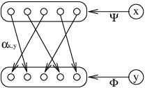
A morphism between two such objects includes morphisms of the form (32) between the objects of and ; this gives bijections between the underlying sets which must be compatible with those which are part of the objects (of the form (45)) themselves. The general result is illustrated in (46) and an example appears in figure 9.
| (46) |
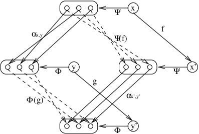
So the naturality square (44) means that the inner square of set bijections in (46) commutes: in other words, that we have given a way to identify all these underlying sets. We can see this in the figure as the fact that following strands of the set bijections (of 3-element sets) around the square reveals that there are exactly three complete squares of strands.
5.1.3. Stuff Type and Fock Space Inner Products Related
The key example of the inner product which makes clear the connection with the inner product on Fock space developed in section 3.1.2 is the inner product of stuff types and , which also happen to be structure types. The stuff type (in fact, structure type) is the type of total orders on an -element set, or “being a totally ordered -element set”. An object of the inner product groupoid is thus a pair which are - and -element totally-ordered sets respectively, equipped with an isomorphism between the underlying sets. We may think of these as the sets and , and the isomorphism is just any bijection between these. If , there are no such objects since there are no such bijections. If , then there are such bijections, given by the permutations of . The morphisms of are just the identity morphisms on these objects, since the only morphisms in the groupoid of totally ordered sets are order-preserving bijections - that is, objects have no nontrivial automorphisms. Thus, we get:
| (47) |
where is the groupoid with objects (one per permutation of ) and only identity morphisms, and is analogous to the usual Kronecker delta, being a groupoid with no objects if and with one object and one morphism if . Thus,
| (48) |
so that the inner product we found on Fock space is natural in this setting. This also illustrates the reason for the factor which shows up in the term in the expansion of a structure type, or the power series which is its generating function. This is the cardinality of the group , the group of permutations of the underlying -element set.
5.2. Stuff Operators
So far we have described stuff types, and implied that they, as extensions of structure types, are a useful way of categorifying functions - in the setting where these functions are seen as states of a certain quantum system. The inner product defined in section 5.1 gives these some of the structure of a Hilbert space, and also makes a connection to Feynman diagrams for energy quanta of a harmonic oscillator. We want to describe more of the structure of the 2-rig of stuff types - in particular its linear structure, demanding a definition for the equivalent of a linear operator. We call such a thing a stuff operator. There will be a category of these, called , with higher-dimensional algebraic structure similar to that of the algebra of linear operators on a Hilbert space, with an action on the category .
We need to describe this action: a stuff operator , given a stuff type , ought to produce another stuff type , using natural category-theoretic operations, in a way that reflects the fact that is the categorified equivalent of a linear operator on a Hilbert space of states. One way to motivate our approach to constructing this is to remember that for a Hilbert space , a linear operator can be thought of as an element of the tensor product of with its dual, and given a basis of , can be represented as a matrix (a two-index tensor). To put this into the same framework as the stuff type , recall that this can be seen as a vector in a space of states33 3 Strictly speaking, the “ground field” here is not but rather the setting for cardinalities of groupoids, , so we do not yet have a vector space. When we introduce -stuff and get cardinalities in something like , we will really have a vectorspace., and the equivalent of resolving it in a basis arises by taking the preimages of elements of as the components in the basis. In this setting, applying to a vector (using the in the description in terms of ) amounts to applying covectors in any decomposition of to , which (since ) amounts to taking the inner product of with a vector in . Since we have already seen a natural definition of inner product for stuff types, we will use a similar construction.
A stuff type can be variously seen as the projection map of a groupoid-bundle on finite sets, and also as a way of picking out an index for some component of a vector in a categorified equivalent of a Hilbert space. A stuff operator should have two such maps, since it is to correspond to a linear operator. We should think of this as “resolving in the same basis”.
The analogy with matrices suggests that acts on stuff types in the same way as the inner product, just as matrices act on vectors (resolved in a basis) by way of the inner product in each index. So indeed, is defined as a weak pullback:
Definition 18.
A stuff operator is a groupoid with two projection maps into :
| (49) |
We have seen the internal picture of objects of in figure 4, so we next look at a similar description for . An object is somewhat similar to an object of , but this object has not just one underlying set, but two possibly distinct ones, which we call and , which in general need not have the same cardinality. We can think of this as two sets sharing a common label, which we may think of as a “process” connecting with , where the label contains stuff associated to this transition, shown generally in (50) and illustrated in figure 10.
| (50) |
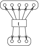
We are not yet at the point of recovering Feynman diagrams, but we can already see an object which contains some sort of label for a process connecting an -element set of “quanta” (in the convention we have already applied to the harmonic oscillator) to an -element set of “quanta”. First we should see how these act like linear operators.
We can define an algebraic structure of stuff operators, when we recall how the the categorical product and coproduct work for groupoids and in . The coproduct is just the direct sum of groupoids, whose objects and morphisms are all objects and morphisms of either or (in a way which distinguishes where they came from). Their categorical product of has objects and morphisms both consisting of ordered pairs of those from and . We have seen that these operations are compatible with groupoid cardinalities.
Definition 19.
Given two stuff operators , with projection operators , and , , respectively, the sum has groupoid whose projection functors act like or as appropriate. The product of by a groupoid , has objects is the product groupoid (with projection operators acting on the component).
These naturally have the properties that and in the sense of the sum and “scalar product” of stuff types, and thus the corresponding facts hold “on the nose” (i.e. as equations) for cardinalities. On the other hand, if we think of the stuff operators as the categorified equivalent of infinite matrices (with projection operators the equivalent of indexing), we can think of these as the sum and scalar product for matrices, defining the linear structure of the algebra of operators. We leave the proof of this to the interested reader.
More interesting is its internal multiplication, and the action on our categorified Hilbert space, the 2-category .
Definition 20.
There is also an action of on a stuff type giving a stuff type given by a weak pullback:
| (51) |
and a composite of and given similarly:
| (52) |
Here, we note that , which can be seen by considering the isomorphisms of the weak pullbacks in the diagrams for these two constructs.
Now, the groupoid resulting from the action of naturally becomes a stuff type (a groupoid over ) by composition of the projections , where is the projection onto from , which is the pullback of the functor from onto along the projection from to the same copy of . To understand this construction better, we should see what the objects and morphisms of the groupoid are like internally.
The stuff type is a weak pullback of and , over the copy of which is the target of , and also of . Its objects will be pairs of objects and together with isomorphisms . These are isomorphisms of the underlying sets, so in particular they only exist if these sets have the same cardinality. Thus, an object of looks like an object of connected by a bijection of underlying sets to an object of (using the “right-hand” underlying set of ). The general form is shown in (53) and an example is illustrated in figure 11.
| (53) |

Since this is to be an object of , we should see it as a stuff type it its own right, over the copy of mapped to under the projection from . That is, everything in this picture - the object, object, and the specific bijection between the appropriate underlying sets - can be regarded as “-stuff” attached to the underlying set .
Now as for the composite of and , similar reasoning holds except that we have another stuff operator in place of , so the general form of an object of is as shown in (54), and an example is illustrated in figure 12.
| (54) |
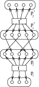
The construction we have described for stuff operators is an example of a “span”: in particular, as morphisms from to itself. The composition we have described above, as well as being analogous to matrix multiplication of linear operators, satisfies the axioms for composition of morphisms. But in fact we have seen that these operators also have an action on the category , derived from the fact that it is a category over . In fact, we can interpret stuff operators as endofunctors of , just as linear operators are endofunctions of a vector space. We describe this in more detail in appendix B.1.
5.3. Feynman Diagrams and Stuff Operators
From a quantum mechanical point of view, we are often interested in finding inner products such as , and finding these inner products can be done by means of Feynman diagrams. That is, in QM, the “transition amplitude” between states and is a sum of amplitudes associated to Feynman diagrams, each showing one possible way of getting from state to state by process . We will show how this idea can be recovered in the categorified setting, and in fact is given by exactly the algebraic ideas we have defined. In general, the groupoid has objects as shown in figure 13

We will see that we can think of these as Feynman diagrams, and finding the sum over their amplitudes is exactly the process of taking the groupoid cardinality of this inner product of stuff types - that is, a sum over Feynman diagrams of some “amplitudes”. At the moment, these amplitudes are all positive reals, rather than complex numbers as is usual in quantum mechanics. When we discuss -stuff types in section 6, and in particular the case in section 6.2, we will see how this can be resolved by introducing the quantum mechanical notion of phase.
Since we are motivated here by the use of the algebra of stuff types as a categorification of the Weyl algebra, we examine the stuff operators and , the annihilation and creation operators. The annihilation operator can be realized in this form, with with two projection functors to , one of which is the identity, the other of which is the functor whose action on objects is to take a set and produce :
| (55) |
To see that this reduces to our previous definition for (definition 7) on stuff types which happen to be structure types, first recall that it said an -structure on a set is an -structure on the set . If our stuff type happens to be a structure type whose groupoid is just a set of -structured finite sets, then we have:
| (56) |
Tracing the map in the new type from to , we note that we can pass through so that , in which case we see that since must make the lower triangle commmute so that we get that the preimage of a given finite set under must correspond to the preimage of under . So indeed, putting an -structure on amounts to putting an -structure on .
Similar reasoning shows that , the adjoint of , can be realized in the same way, with groupoid but with the projections reversed:
| (57) |
Moreover, this acts like , so that in the event that is a structure type, a -structure on a finite set amounts to choosing an element of and putting an structure on what remains.
From the parallel with Fock space, one operator we should want to define is the field operator . As a stuff operator, this behaves as one might expect: the groupoid in the stuff operator is just the groupoid sum (i.e. two copies of ), and the projections just act as the projections on and when applied to objects and morphisms from each of the two copies. So, the objects of the groupoid , following the pattern we illustrated in (50), look like either objects of or of , as shown in figure 14.

In our categorified setting, this is written nearly the same way, , but we now have an interpretation of the inner product as a groupoid over , obtained by a pullback - and indeed, of the stuff operator as a composite of stuff operators, etc. Now, this has objects which are chains of objects of the form in figure 14, composed as in figure 12. We can draw these in various ways (different drawing styles form objects in equivalent categories), but for compactness, we will draw these in a style which omits the “internal” bijections of the composite type, and also the bijections from the and objects of to . Thus, each internal finite set would have previously been drawn three times, with bijections between them. This compact style is illustrated in figure 15, which shows an object of . This one shows an object made from one annihilation and three creation operators, in that order. All other permutations of four -objects are possible also.

For the sake of further compactness (and another drawing style depicting an equivalent category), note that what we really have here is an operation in which quanta of energy either appear or disappear, and do so in a definite order. We could really draw this with just a single “interaction” vertex, incident with strands (all other strands passing straight through the diagram, matching up a quantum in the top with a quantum in the bottom). These incidences would have to be labelled with a total ordering, so that the object shown in figure 15 would be drawn as in figure 16.

There is an action of the permutation group on these objects, changing the order in which we encounter objects from and as we pass through . That is, for every object we get whose diagram has one order labelling the incidences, we will get objects with all other possible orders exactly once through the action of the permutation group , also known as . So if we want to omit this labelling for clarity in the drawings, we can do so as long as we remember that this means we are really drawing objects of the weak quotient (weak quotients are defined in definition 12). The objects of this weak quotient are isomorphism classes of diagrams under permutations of labellings. These permutations give the natural isomorphisms in the definition of weak quotient by taking any labelled diagram to the same diagram with permuted labels. In this new category, the cardinality of the groupoid is thus scaled by . We also need to keep in mind that an unlabelled diagram really stands in for possibly several different inequivalent labellings of the incidences by distinct orderings.
All this is really a notational convenience: really, to calculate transition amplitude between states and for which we have a description as stuff types and , when we put the system through some process which we describe as a stuff operator , we only need to find the groupoid cardinality . Simplifying diagrams and finding convenient conventions for labelling them is really a way for getting a calculational convenience out of diagrams like figure 17, which shows an object from the groupoid .

Now, diagrams like this give vertices with incidences. Taking polynomials in the operators which give such diagrams gives operators which can be interpreted in terms of diagrams having several such vertices. Such a diagram is shown in figure 18 - note that here we continue the practice of omitting to draw the internal finite sets in the composite stuff operator.

Given two stuff types and , we can take the inner product . This applies this operator to to give compound objects involving objects of and of . Taking the inner product with gives objects as illustrated in figure 18. The groupoid cardinality of this inner product amounts to a sum over all such diagrams, each with a weight related to the size of the symmetry group of the diagram.
Example 13.
We can use the above to show the categorical meaning of the usual calculation of the expectation value of a power of the field operator. In particular, suppose we want to calculate , the vacuum expectation value of the 6th power of the (normalized) field operator.
To do this, we want to take a sum over objects which are equivalent to ways of matching two empty sets with diagrams like figure 17, containing one vertex of valence 6. We begin with the case where incidences are labelled (as in figure 16). Since the source and target sets are empty, all edges must form loops touching the vertex at both ends. The number of such diagrams is (choosing the endpoints of three edges, without order). These give the objects of a groupoid one of which is shown in figure 19.

The isomorphisms of this groupoid are given by permutations of the labels. Since this permutation group is with elements, the groupoid cardinality should be . The automorphism group of any such diagram is of size 48: there are 6 ways to map the set of loops to themselves, each with the same orientation, or reversed orientation. Equivalently, we can think of the objects of the groupoid as diagrams like this, but without labels. In this case, there is only one such diagram, with the automorphism group as just described. So we have .
Now, the transition amplitude between two states in a quantum harmonic oscillator which undergoes an interaction described by a given operator in the Weyl algebra can be calculated, in part using a sum over Feynman diagrams. We have now seen how, in this categorified setting, we can find a direct combinatorial interpretation for this fact.
Unfortunately, some features of the diagrams used in quantum mechanics are missing from this interpretation. In particular, we do not have any way to express the notion of “phase”, or operators involving propagators without interactions. In quantum mechanics, states exist in superpositions - linear combinations - having complex coefficients. Non-interacting propagation in time involves the rotation of those coefficients by a phase - that is, a unit complex number. Thus, both and the group of phases are important. We will see in section 6 how to incorporate this into our combinatorial picture. As we shall see, this involves an explicit decomposition of complex numbers into amplitudes and phases.
6. -Stuff Types And Quantum Mechanics
We have described various entities under the heading types, namely stuff, structure, and property types, and hinted at the possibility that this sequence of classifications will continue as we move into the setting of increasingly higher-dimensional categories. For physical purposes, though, we are still missing some essential properties which we would like a categorified version of quantum mechanics to have. In particular, all of our cardinalities, and hence coefficients of our types, lie in rigs, rather than rings - they can be added and multiplied, but not subtracted and divided. It is possible to handle this in the abstract setting of structure types by defining virtual structure types as equivalence classes of formal differences of structure types (and similarly for stuff types) to make subtraction possible (see [3]). For quantum mechanics, however, the coefficients of the power series which represent states are complex numbers, and the physical significance of phase is of paramount importance, so we will still need something more. So for our purposes, it makes more sense to treat the question in a different way.
6.1. -Stuff Types
Now we will see an analog of a stuff type which can carry a phase - or more generally, a weighting of some kind. To reproduce some of the features of quantum mechanics which don’t appear in the picture of stuff types as “categorified states”, we should consider what is missing. First, states of a quantum system should form a Hilbert space, and in particular a vector space. Since we already have something like an inner product, what is missing is the ability to take linear combinations of states. For this, they need to have a notion of scalar product and of addition. If we allow the categorified states to carry a weight, this weight can play the role of a scalar multiple, but these weights need to form a monoid, which we think of as multiplicative.
This is the motivation for defining a notion of “-Stuff Types” for some monoid , and in particular , the group of phases. This is the case which is most interesting for quantum mechanics. We’ll do this in general, since the construction does not require .
6.1.1. -Sets
Before we can talk about -Stuff Types, we should start with a more basic definition:
Definition 21.
If is a monoid, is the category of “sets over ’’44 4 See appendix B for comments about such “over categories”. The usual definition applies here by treating as a set of elements, though we get some extra structure from the monoidal operation on ., or “-sets”. Its objects are pairs , for and . Morphisms between two -sets and are maps in giving commuting triangles:
| (58) |
By abuse of notation, we will sometimes call the object just or just if the meaning is clear by context. A similar definition can be made for or , where the sets lie in or .
Note that for each set of cardinality , the set of all -sets with “overlying set” is just , equivalent to . The morphisms which make this into an over category provide some extra structure, however.
We also note that this definition is similar to that for a -coloured set for a groupoid - in fact, the image one should have of an -coloured set is just the same as figure 2. One difference is that in this case, the picture we have for morphisms is different from that for -coloured sets: for -Sets, morphisms are just set maps which are compatible with the labelling. We could, of course, define a weak over category of sets “weakly over ”, as we did with groupoid-coloured sets, for which strands of morphisms are also labelled by elements of , but as we shall see, this is not what we want to do. One result of this is that we lose some of the desirable features of the category of sets, while retaining others. For example, we have the following:
Theorem 7.
is a category with all colimits (in particular, it has coproducts).
Proof.
First, consider any diagram in , and take the underlying diagram in . Since is a cocomplete category, every diagram, and in particular this one, has a colimit . The diagram in has a colimit provided we can construct a map from to which is compatible with the set-maps from the objects of the diagram in . For any given element in , every element taken to it by one of the maps in must have the same image in under the map for the corresponding object in , since if there is more than one, they must be taken to some common element by maps in the diagram. Thus, we can consistently define for any element in the colimit to be equal to the value for any preimage, and so all the maps in are compatible with the function into , and the colimit in becomes a colimit in . ∎
Coproducts in can be interpreted as direct sums of -sets - and this makes it possible to define a cardinality for -sets. We note that since has only one monoidal operation, we could consider two interesting kinds of cardinality, depending on whether we want this operation to look like addition or multiplication.
For our purposes, it is better to think of as a multiplicative monoid, since we will later want to take , thought of as a subgroup of . So we would like to have a notion of cardinality which gets along with multiplication in an analogous way. We should define a notion of cardinality which reduces to set cardinality when we think of as multiplicative. Then we will find a “tensor product” compatible with this notion of cardinality.
Definition 22.
The cardinality of an -set is an element of given by
| (59) |
where the sum is taken in .
This cardinality operator is a kind of decategorification: it takes a set labelled with values in , and gives a formal sum of values in , each taken the number of times it appears in . Note that this is again not compatible with the cartesian product in , by the same argument as for the additive cardinality. Instead, we should take the following product:
Definition 23.
The tensor product of two -sets and is an -set has underlying set (the cartesian product of underlying sets in ). The map is given by .
Theorem 8.
The tensor product of -sets satisfies . When is commutative, the tensor product is symmetric.
Proof.
| (60) | |||||
When is commutative, there is an obvious isomorphism between and taking to ; the labelling is unchanged, since . ∎
These constructions for sets can be extended to groupoids, where cardinalities start to look like complex numbers.
6.1.2. -Groupoids
We would like to extend these results about -sets to a notion of -groupoids and their cardinalities which is compatible with cardinalities of -sets and of ordinary groupoids in the suitable special cases. One way to see the correct approach to -groupoids is to take advantage our existing idea of -sets and a connection we already know between sets and groupoids. This is the concept of a groupoid-coloured set. We define groupoid-coloured -sets by analogy with these. Recall from 4.1.2 that a set can be seen as groupoid whose objects are the elements of the set, and with only identity morphisms55 5 Since we are already thinking of sets as special kinds of categories here, this raises the question of what happens if we categorify . We return to this in section 7.1.2.. Then we have:
Definition 24.
Given a groupoid , a -coloured -set is an -set equipped with a colouring map . Maps of -coloured -sets are -set bijections together with, for each ), a morphism . That is,
| (61) |
This is essentially the same definition as appeared in 4.1.2, but we note that now is a bijection of -sets - that is, it is a set bijection which is compatible with the -labelling. But notice that groupoid-coloured -sets are just sets with two maps, one into a groupoid, and one into a monoid:
| (62) |
Since the elements of this -coloured -set are just elements of labelled by both an object of and an element of , we would like to be able to think of this as a set labelled by objects of an “-groupoid”, which would look like objects of the groupoid labelled by element of . A consideration of what morphisms of -coloured -sets must be reveals how to define this:
Definition 25.
Given a monoid , an -groupoid is a groupoid with a functor from into the set regarded as a groupoid. The cardinality of an -groupoid is an element of , where and are thought of as multiplicative monoids. The cardinality of is given by the formal sum:
| (63) |
Remark 6.
Note that consists of all formal -linear sums of formal products for and , subject to the distributive law . It becomes a rig with the obvious multiplication .
Since we are thinking of as a groupoid with only identity morphisms, functoriality of means that for any and in and , we have . That is, the following diagram commutes:
| (64) |
We see also that is well defined for elements of any given isomorphism, since any two objects with an isomorphism between them will be sent under to the same element of . It should be clear that in the case where the “overlying” groupoid of an -groupoid happens to be a set (i.e. groupoid with only trivial morphisms), this reduces to the definition of an -set and its cardinality. In the case where is the trivial groupoid, this cardinality reduces to the usual groupoid cardinality.
Given two -groupoids, we define their product as with -sets:
Definition 26.
The tensor product of two -groupoids and is an -groupoid which has underlying groupoid (the cartesian product of underlying groupoids in ). The map is given by .
As with -sets, this product gets along with -groupoid cardinalities. The proof is essentially the same, except that cardinalities involve factors of . This depends on the fact that the automorphism group of an object in is just the product of the automorphism groups of and .
6.1.3. -Stuff Types and their Cardinalities
We begin with a definition:
Definition 27.
An -stuff type is an -groupoid equipped with a functor , where .
Typically, we will just think of as an object of and blur the details, but this definition is what we always mean. So as with stuff types, we may think of -stuff types as functors from -sets of “-stuffed finite sets” to their underlying finite sets. In the case where is faithful we can say it is an -structure type. Note that we are still thinking of as lying over , not - we will return to this shortly.
Since stuff types (and -stuff types) can be multiplied by groupoids, whose cardinalities lie in , this action by gives another version of multiplication. This will be particularly interesting when we consider in section 6.2, but first we should define the cardinality of an -stuff type:
Definition 28.
The cardinality of an -stuff type is
| (65) |
where is now the -groupoid cardinality of the preimage of under .
(As with a stuff type, this definition requires us to take to be skeletal to be well defined - or else to consider only the essential preimage. We will do the former.) This cardinality is an element of : a formal power series in whose coefficients are formal combinations of pairs of groupoid cardinalities and elements of .
Theorem 9.
There are natural left and right actions of the monoid on the -stuff type . If is abelian, these are the same action, which satisfies
| (66) |
Proof.
We define the map , where acts as follows. If is an object of whose weight is , then the corresponding element in has weight . Then . This is a left action on stuff types because it is a left action on -groupoids together with a compatible map to . The right action of is defined similarly.
If is abelian, a left and right action are the same, and the result follows by direct calculation. ∎
6.1.4. -Stuff Type Inner Product and -Stuff Operators
Once we defined -sets and hence -groupoids, it was possible to define -stuff types simply by substituting these for groupoids in the original definition of stuff types. The only properties of which were used in the original construction of stuff types and operators was that it should be a groupoid: groupoids with one or two functors into it were stuff types and operators respectively. Morphisms between the objects of a stuff type were morphisms in together with compatible bijections of sets (recall figure 5), but this depended only on the fact that these were isomorphisms in the groupoid . So, in the same way, a morphism in the groupoid of an -stuff type consists of a morphism in its -groupoid, together with a compatible bijection of underlying sets, as illustrated in figure 20. Notice that the objects and are labelled by the same element, , since is an isomorphism in .

Now, the inner product of stuff types and was defined to be a weak pullback, as described in (43). The same definition will apply if we let these be -stuff types, allowing and to be -groupoids.
So we have a weak pullback of along , which gives a groupoid , and can define canonical projection maps to and . The groupoid is the fibrewise product , where we must use the tensor product of -groupoids rather than the cartesian product of groupoids to assign elements of to its objects.
Definition 29.
The given two -stuff-types , and , the -groupoid is the weak pullback of and over . It has objects which are pairs equipped with an isomorphism . A morphism in is a morphism in , say , such that
| (67) |
commutes. That is, .
An object in the inner product groupoid looks like figure 21, where are elements of . This figure is analogous to the previous inner product (figure 8). Note that, in contrast to the case in figure 20, the objects and are not in the same groupoid, hence not related by any morphism, so there is no requirement that and should be equal. The object illustrated is labelled be the element (as highlighted).

Similar changes apply to the other constructions defined using the weak pullback, so that we have nearly identical categorical diagrams definining morphisms in the inner product, as well as the action of an -stuff operator on an -stuff type and the composition of two -stuff operators, as in definition 20. The sole change at this level is the replacement of groupoids with -groupoids, and thus in figures 11 and 12, we have labels in on every groupoid object, preserved under every isomorphism.
Definition 30.
An -stuff operator is an -groupoid with two functors from the underlying groupoid of into :
| (68) |
It acts on an -stuff type to give another -stuff type by weak pullback over one copy of .
Just as with the former constructions, we have:
Theorem 10.
If and are two -stuff types, then .
Proof.
At the level of the underlying sets and groupoids, every product over a finite set in the (skeletal version of) in the fibrewise product looks just the same as for regular stuff types. Each of these products is a product of -groupoids, which are compatible with cardinality. So the result holds. ∎
6.2. Quantum Mechanics:
As remarked earlier, the notion of a phase is crucial in quantum mechanics. Stuff types, and in particular stuff operators and the inner product of stuff types, proved in the last section to have a close connection to entities which resemble Feynman diagrams, but the only notion of cardinality we had for these was groupoid cardinality, which yields positive real values. We would like to be able to do more, since in quantum mechanics, these diagrams should have not a real cardinality, but a complex amplitude, which has both a magnitude and a phase. This leads us to the idea of -stuff types, since is the group of phases, corresponding to the unit circle in .
6.2.1. -Stuff Types
From here on, we take - an abelian monoid, and in fact an abelian group - we know that -stuff types exist, and that they have cardinalities in , which has the obvious homomorphism into . As we have seen, the cardinalities of -sets for an abelian monoid lie in , which we can think of ; cardinalities for -groupoids lie in ; cardinalities for -stuff types lie in . When , this gives , which has a homomorphism onto
| (69) |
We should note that this description of in terms of explicitly separates complex numbers into a magnitude and a phase, and while it has a multiplication resembling that for , but it fails to capture the addition, which is formal. However, the homomorphism just imposes the relations which define complex addition. The derived rig homomorphism behaves similarly. This homomorphism loses information, just as the process of taking cardinalities does, so in fact, when , we can define a new cardinality operator:
Definition 31.
If is a -groupoid and a -stuff type, the complex cardinality of is applied to the usual -stuff-type cardinality:
| (70) |
where is the usual -stuff cardinality, is the above homomorphism, and addition is in .
The complex cardinality is a map which takes a -stuff type and yields a power series in , namely Fock space. When dealing with -stuff types, we will write as , unless otherwise noted.
Remark 7.
Note that a type which consists of two states over -sets of the same set cardinality but opposite phase will have a cardinality in which contains a formal linear combination which is in the kernel of . This is the critical fact that when we represent states in Fock space, there can be interference between states with opposite phases. In particular, the amplitude for a (categorified) state containing only those two objects will be zero.
6.2.2. Conjugation and The Inner Product
There is a property of -stuff types which is not generally shared by -stuff types for arbitrary , resulting from the fact that it is an Abelian group. This follows from the fact that there is a nontrivial monoid isomorphism between and itself, taking each element of to its multiplicative inverse. There will be such an isomorphism whenever is an Abelian group. Viewing as the unit complex numbers, however, allows us to see this as complex conjugation, which is how we will think of it. Thus, there is an operation special to -stuff types:
Definition 32.
If is a groupoid with labelling , its conjugate groupoid is the groupoid whose groupoid is labelling is , given by . When we write for the -groupoid, we write the conjugate as . If is a -stuff type, its conjugate is the type which acts like on the objects of the underlying groupoid of .
This allows us to define a variant of the inner product which has the conjugate-linearity of the usual complex inner product on Fock space. To distinguish this from the (bilinear) inner product , and call it , also a more familiar notation to physicists:
Definition 33.
The Fock space inner product is given by
| (71) |
Theorem 11.
The Fock space inner product, for -stuff types and satisfies , giving the usual conjugate-linear inner product on .
Proof.
| (72) | |||||
∎
So for -stuff types, we might want to define a new inner product given in terms of the usual -stuff type inner product as . We will discuss briefly in section 7.1.1 how to interpret this seemingly arbitrary innovation.
It is worth noting here that the inner product between two states of a -stuff type may be zero. Of course, this can happen with stuff types in any case: for instance, if is the stuff type for which there is one object in over every even-cardinality set, with automorphism group the same as that of the set, and no others; and is similar, but has objects over odd-cardinality sets. These have cardinalities (generating functions) and respectively. They are examples of what we called “property types” in section 4.4 - namely, these types can be interpreted as the properties “being an even set” and “being an odd set”. These two stuff types are orthogonal in the sense that their inner product is zero. Here, the interpretation is that there are no sets having both properties, and so the stuff-type inner product is the empty groupoid.
However, the situation with -types is more subtle: we may have a nonempty inner product groupoid whose -groupoid cardinality happens to be zero. This arises because we may now have negative (and indeed complex) contributions to the sum giving this cardinality. This is related to the quantum mechanical phenomenon of “destructive interference” between states. In our formalism, this interference occurs when we apply the homomorphism and its derived variants.
We interpret the cardinality of the groupoid inner product as the usual inner product in quantum-mechanics. This is the amplitude for finding our system in a given state after setting it up in a state , so this says this amplitude (and hence the probability) is zero.
So the transition amplitudes between some of the “pure” (decategorified) states of which and are superpositions may be nonzero, but the phases with which they appear may allow the transition between and to have zero amplitude. Thus, introducing phases allows destructive interference which makes otherwise feasible transitions impossible. We will see in the next section that this issue of phase is closely related to the concept of time evolution in quantum mechanics, and the propagator.
In particular, in the harmonic oscillator, the phase of a state changes over time, with a frequency proportional to the energy of that state. This is the effect of the free propagator for a system, and it is an operator. So we must describe -stuff operators next, and this propagator in particular.
6.2.3. -Stuff Operators and Time
We have already noted that -stuff operators act on -stuff types just like ordinary stuff operators acting on stuff types, except that the groupoids are now replaced by -groupoids. The groupoid for an -stuff operator and type then consists of pairs of objects and together with a bijection of their underlying sets. As with the product groupoid, this object is labelled by an element in given by the product of the labels on and . This is well defined when is Abelian, as in the case when .
One class of -stuff operators which is particularly relevant to quantum mechanics is that of the time evolution operators. These are operators which, when applied to an -stuff type , produce an -stuff type for which the -labels on the elements of the underlying sets have labels multiplied by a fixed phase in . An example of an object in such an operator, designated , is shown in figure 22. Here, we are showing the operator , “time evolution by ”. We show an object which will evolve a state with three quanta of energy. Here, is the change of phase corresponding to time evolution of a one-energy-quantum state by . A state with three energy quanta changes phase by .

Any object in has two projections - each to an underlying set of the same size. This corresponds to the fact that in unperturbed time evolution no interactions are occurring which would change the energy level of the system. An object in the groupoid of , lying over sets with quanta of energy. There will be just one such object in for each finite set. It is labelled by the phase by which a state with quanta will change in time . The operator acts on any -stuff type (categorified state) to give state to which this has evolved after a time . An object of the resulting stuff type is shown in figure 23.

The object in the groupoid of is the entire ensemble associated to the finite set . It includes the object itself, as well as , their underlying sets and the bijection between them, and also their associated labels and . This is an object in a product -groupoid: is a weak 2-category with (weak) products, of which this is an example. This object in the product groupoid is labelled by the product of the labels on and , namely .
Suppose the -stuff type in question happens to just be - the categorified state with just quanta of energy and no phase angle, or the property type “being an -element finite set labelled by ”. Then we get , and the same fact holds as an equation for the complex cardinalities. So the -cardinality of a -element -set changes by in time , since each quantum picks up a phase rotation of in time . In particular, the phase of an object in a categorified state changes with a frequency proportional to its energy (the size of the underlying set).
Choosing time units so that , we get a phase change of on a state of energy . We can write this as , where is the number operator. To prove this equality at the categorified level (using a categorification of the exponential such as we have already discussed) would require a fully categorified version of the complex numbers. However, for now we can observe that this will be true at the level of cardinalities, and take it as a definition. This arises physically from the Hamiltonian formulation of quantum mechanics. We will not enter into this in detail, but note that the free Hamiltonian is just , the number operator in the exponent of the propagator, which measures the energy of a state.
Since has exactly one object for each cardinality, the product groupoid is equivalent to the groupoid whose objects are the same as those of , but whose -labellings have been multiplied by phases , for an object with underlying set . This is the groupoid of the state , time-evolved by . Note that time-evolution by will be given by a similar operator : all the object-labels are the inverses of those of . We will return to this point in section 7.1.1.
In any case, using these propagators, and the version of inner product groupoids whose objects resemble Feynman diagram for interactions, we recover a combinatorial interpretation for many of the standard features of the quantum mechanics of the harmonic oscillator.
6.2.4. Feynman Diagrams And Perturbation
Having found a categorification of the quantum harmonic oscillator, we know that transition amplitudes such as as a sum over Feynman diagrams. In physically realistic settings, this sort of amplitude often arises when we consider the time-evolution of an oscillator which is perturbed. The free oscillator evolves in time according to the operator described above. The perturbed oscillator, on the other hand, describes a situation where the energy of the oscillator is modified by another term: it only approximately matches the description of the free oscillator we have been using. Physically, this represents a potential in which the oscillator is moving. This means that the energy of the oscillator is changed by the addition of an extra term, , which is some function of position, which we think of as a potential energy, in addition to the energy in the oscillator proper.
In this case, time evolution can be calculated using the new energy, . If is a function of position, then since the position is proportional to , we have , for some function . We will consider the case where is some polynomial (though naturally any analytic function can be approximated this way to some degree, so we can obtain successive approximations by taking a sequence of converging to ). Since the energy for the free oscillator is already quadratic in position, we assume that has minimum degree at least 3. In this case, at the decategorified level, the amplitudes for time evolution by time associated to the Hamiltonian , are:
| (73) |
To avoid considering questions of convergence, we think of this purely as a statement about power series in . It would take us too far afield to derive this standard quantum-mechanical fact in full detail, though background can be found in [4], and one derivation of this equation in our setting can be found in [2]. However, we will point out here that it follows from the fact that the evolution of a state is governed by the Schrödinger equation, which amounts to:
| (74) |
Integrating this equation over time, we get
| (75) |
and by repeated substitution of this expression for into the integral, we get the sum of integrals which appear in the expression above. Taking the inner product with this operator, we finally get the whole expression.
Ideally, we would like to derive this equation entirely at the categorified level. However this would require a more complete understanding of the categorified version of the complex numbers than we have constructed here. To recover time evolution by a phase from an expression of the form , we would need to see that the result is indeed a phase in .
However, knowing that the equation holds at the decategorified level allows us to give a simple interpretation for the formula.
Theorem 12.
The transition amplitude for the perturbed harmonic oscillator with potential is given by a sum over all Feynman diagrams given as composites of those associated with , from a state with quanta to one with quanta. The sum is of an integral over all labellings of the edges of the diagrams such that the total phase along all paths is .
Proof.
This transition amplitude is the -groupoid cardinality of the inner product , and given by 73. Consider the operator in that equation,
We know that the terms are just free propagators, which contribute a phase of for each quantum of energy. We can think of these operators as having objects given by any number of “strands”, one for each quantum, and each strand labelled by a phase , the total number giving the total phase change associated to that energy.
Now consider the -stuff operators . Each of these operators has a groupoid whose objects are naturally identified with Feynman diagrams of the sort associated with . These do not affect phases.
Composing the operators together, we get all possible composites of Feynman diagrams of the type associated to , connected by diagrams whose effect is to label strands by phases associated to the time intervals between interactions. To find the total phase associated to such a composite, we multiply all phases. This is clearly equivalent to multiplying the phases on any labelled edges which are joined by the composition to get a phase on the resulting edge, then multiplying the product of all edges thus produced.
The transition amplitude we want to recover is:
The sum taken over all simply means that we are taking a groupoid containing all possible -fold composites of this form. The integral over all -part partitions of the interval means each such diagram contributes a phase found by integrating over all possible ways of dividing the interval into free and interaction parts. This contribution is weighted by the size of the symmetry group, since the inner product inside the integral is just a -groupoid cardinality.
This proves the statement. ∎
This recovers the usual Feynman rules for calculating transition amplitudes in the oscillator.
7. Conclusions
Here we summarize what we have shown, and suggest directions in which this work could be carried further.
7.1. Categorified Quantum Mechanics
We began by describing the quantum harmonic oscillator and the Weyl algebra, the algebra of linear operators on its space of states which correspond to observables and interactions of the oscillator system. We saw how this could be related - by the Fock representation of the Weyl algebra - to formal power series with complex coefficients with exponents counting quanta of energy.
Our aim at the outset was to categorify this aspect of quantum mechanics. Categorification of concepts such as “group”, “vector-space”, and indeed “category” itself have proved interesting within mathematics, and the resulting 2-groups, 2-vector-spaces, and 2-categories arise naturally in surprising ways. The idea here was that categorification could be applied in a physically relevant setting, and could reveal something useful about the mathematical structures involved. Here, we began with the Hilbert space of states of a quantum mechanical system, and the relevant algebra of operators acting on it. We have produced category-theoretic equivalents of these: the 2-categories of stuff types and of stuff operators can be seen as a categorified Hilbert space and a categorified algebra.
These are connected to the original setting by concepts of decategorification which go by the name “cardinality”. We have shown that when we take the cardinalities of all our entities involving “stuff”, we recover much of the structure of the Weyl algebra. By introducing the idea of -sets, and attendant ideas of entities labelled with “phases” from some monoid, we have improved this resemblance to quantum mechanics.
Stuff types - groupoids over - have creation and annihilation operators which give a purely combinatorial construction which categorified many features of the Weyl algebra. They also have a natural inner product which, in conjunction with these creation and annihilation operators, allows us to interpret transition amplitudes as sums over Feynman diagrams.
However, what these categorify is not Fock space, since it only has scalar multiplication over , rather than , and cardinalities in , rather than . Our -stuff types are a better categorification of Fock space, and these have cardinalities in , which we can map to . This map is not one-to-one, and this fact is responsible for the phenomenon of interference of states with different phases.
The problem of categorifying quantum mechanics is much more general than the simple case of a harmonic oscillator we have discussed. Another approach to bringing category theory to quantum mechanics is [5]. That paper provides good description of a simple “picture calculus” for quite general quantum mechanics which uses a background of category theory. This is not a categorification in our sense, but together with some of the structure described in appendix B may suggest a broader framework for dealing with the question.
Although we have confined ourselves to the harmonic oscillator in this paper, we can suggest various directions in which these ideas could be taken further. One is to look at the inner product through a more category-theoretic lens.
7.1.1. Conjugate-Linearity and the Inner Product
Recall that the inner product for -stuff types had to be modified somewhat in order to agree with the usual inner product on the Hilbert space in the case when . The nontrivial isomorphism of with itself provides a notion of complex conjugation. But how should we interpret the inner product for -stuff types?
In fact, it makes more sense when we adopt the interpretation of the inner product as pairing a state vector with a costate covector. So the (conjugate-linear) inner product gives the amplitude to find a system set up in state and evolving according to the operator to be measured in state . This suggests we should think of observing a system in a certain state as a time-reversed version of setting the system up in that state.
But if time evolution by is given by an operator , time-evolution by is described by an operator . This has groupoid and projections to the same as those for , but the groupoid has objects labels by inverses of the labels on the objects of . In , this inverse is the same as the complex conjugate, so that . This suggests an interpretation of the complex conjugate as a time-reversal of the original stuff type, consistent with our interpretation of a measurement process.
7.1.2. Categorifying
The operation takes two objects in a category and yields the set of morphisms between them. In an enriched category, this can be replaced by some other kind of collection of morphisms - a vector space, for instance. In the case that this collection is always an object of the same category as the original objects, we have a “-object”. In any case becomes a functor into the category in which -objects are found.
Moreover, the functor is a covariant functor, while is contravariant - that is, a (covariant) functor to . This seems closely analogous to the conjugate-linearity in the complex inner product on a Hilbert space. We may ask whether the inner product on a Hilbert space comes from some ? In particular, in order to make a category where morphisms are spans (see appendix B), we need to look at the opposite category of a -groupoid. A groupoid is indistinguishable from its opposite category after taking cardinality - but what about an -groupoid?
To make sense of this idea, we could replace a monoid with a monoidal category, . A groupoid with objects labelled in the monoid - that is, with a function from its set of objects to , would be replaced by a groupoid with a functor into the monoidal category - so in particular, we would have labellings of morphisms of with morphisms of . This combination of groupoid and functor can be interpreted as an object in the category of “groupoids over ”.
Given a categorification of , we could ask whether this new setting more naturally produces the inner product we want for quantum mechanics. So far, though, we have not considered how to categorify the group of phases in order to accomplish this most naturally.
7.1.3. Non-Counting Measures and -Groupoid Cardinality
We saw in equation (73) and what followed that the transition amplitudes for the perturbed harmonic oscillator are given in terms of a sum and integral over all Feynman diagrams with edges weighted by phases. To do this, we had to accept the equation at the equational level and then give it an interpretation in terms of -stuff types, since we have, to date, not given any categorified meaning for the integrals. We can observe, however, that our notion of cardinality for -groupoids, and by extension -stuff types, used only the groupoid cardinality derived from counting measure on sets, weights from the monoid .
To give a categorified interpretation of the integral directly, we might wish to use the fact that when , there is a measure other than counting measure on itself. In this case, the natural choice is the Haar measure on the Lie group - though for other choices of there may be other natural choices. Then a cardinality operator for an -groupoid would involve an integral involving both and the groupoid structure. In the case where the measure on is just set cardinality, this should reduce to the more combinatorial definition given here. We could hope that such a notion of cardinality would let us give a direct categorified interpretation of equations such as (73).
7.2. Other Generalizations
7.2.1. Higher-Valence Stuff Operators
We have described stuff types and operators in terms of quantum mechanics, but it should be clear that they also have an independent interest as algebraic objects in their own right. Stuff types form a categorified Hilbert space, but also a categorified algebra, since they have a concept of multiplication in the space.
The key fact behind our approach has been that stuff types and stuff operators form 2-categories of groupoids over either one or two copies of . Stuff operators have an action which are the equivalent of linear operators on this 2-Hilbert space. This action arises because of the fact that taking a pullback over one copy of under both a stuff type and an operator removes two of the maps to this underlying , and gives an object with one such map.
In fact, there is no reason why we must restrict ourselves to groupoids with either one or two maps to - the categorified versions of vectors or matrices. We have done so because these are the most directly relevant to quantum mechanics, but for categorified algebra, it makes sense to generalize to look at the equivalent of “-forms”, or “-index tensors” (the natural inner product obscures the difference between vectors and covectors in this setting). These would be groupoids with projections into copies of . Contraction of two tensors over some pair of indices would amount to identifying the corresponding copies of and taking a pullback of the two projections into this copy.
The categorified -forms could be seen as -sort types: types of structure (or stuff) which could be put on underlying sets of different “sorts” of objects.
The notion of a club described by Max Kelly in [8] can be seen as a significant generalization of this setup, where the categories involved need not be groupoids. There is a body of results about these which may bear on the ideas above, and turn out to be relevant to other physical situations.
7.2.2. Multisort Species and QFT
In appendix C.1 we refer to a description of generalized species as functor categories between and for groupoids and . These “species” are the “structure types” of our terminology, which correspond to the case where both groupoids are , the one-element groupoid, in which case and . These correspond to functors from finite sets to sets of structures which can be put on them. We also mentioned the 2-rig , a.k.a , the 2-rig of -sort structure types: these correspond to functors from collections finite sets of “sorts” (i.e. copies of ) to sets of structures which can be put on these.
We could reverse this point of view in the case of structure types, to view them as faithful functors from groupoids of structures into the groupoid of finite sets (giving the “underlying” set of a structure) and then weaken the requirement that the functor be faithful to get the more general “stuff types”, so too we can reverse our point of view of multisort structure types, to view them as faithful functors from a groupoid of “-sort structures” down to , giving the underlying sets of each sort. These functors will be faithful for the same reason as in the case . Weakening this requirement would give us a notion of stuff type corresponding to functions of more than one variable. Defining creation and annihilation operators on each sort of element would let us define a Weyl algebra for sorts of particles - that is, the algebra of operators for quantum harmonic oscillators. This is interesting, since a quantum field theory may be represented as a collection of harmonic oscillators.
Replacing the various sorts of finite sets with finite sets over monoids - in particular, over , as in our discussion of -stuff types - we may find an elementary categorical description of a simple QFT. Further research in this direction may prove fruitful.
7.2.3. Beyond
We have described the 2-Hilbert space of categorified states (stuff types) and 2-algebra of operators (stuff operators) for the categorified quantum harmonic oscillator in terms of some over categories. The 2-category is the slice category of over the groupoid , while the 2-category is the slice category of over .
The groupoid appears in both of these cases, in the fact that it does allows stuff operators to act on stuff types by means of pullbacks. But the 2-Hilbert space structure of does not depend on the fact that the groupoid it lies over is : the linear structure is inherited entirely from the direct sums of groupoids, and the inner product depends only on the fact that any two stuff types and are groupoids over the same groupoid , and thus that we can find a groupoid by taking a weak pullback over .
Similarly, the algebraic properties of - its linear structure, composition, and action on - derive from and the possibility of forming pullbacks. We could derive the same structures for the 2-category of groupoids over for any groupoid . What’s more, just as not all matrices need to be square, and linear transformations needn’t be endofunctions on some single vectorspace, we could take two different groupoids and , and take the 2-category of groupoids over . We could compose these in the obvious way, treating them as “spans” between and - and also as functors between categories of groupoids over and just as stuff operators are endofunctors of groupoids over .
Why did we choose the specific groupoid (or its -coloured counterpart) for the constructions we actually studied? Because its decategorification is , which is the spectrum of the number operator for the quantum harmonic oscillator. This may suggest how to find other groupoids for which these constructions have some particular physical interest. Indeed, as remarked before, Kelly’s theory of “clubs” ([8]) generalizes our framework by, among other things, allowing categories which are not groupoids. Perhaps phenomena related to groupoids can be found which can be given a treatment like the one we have given for the oscillator.
8. Acknowledgements
This work grew out of the regular Quantum Gravity seminar taught by John Baez at UCR, notes for which are available online as [2]. I would like to acknowledge his work on this subject (some published as [1]), excellent teaching, and helpful advice and discussions in preparing this paper. Other students in the seminar, especially Toby Bartels, Miguel Carrion-Alvarez, Alissa Crans, and Derek Wise also provided many useful discussions.
Appendix A A Little Higher-Dimensional Algebra
Definition 34.
A rig, or semiring, is a set with two operations, which we customarily denote by and , referred to as addition and multiplication respectively, such that is a commutative monoid with identity , is a monoid with identitiy . We also require that multiplication distributes over addition on the left and right, and is fixed under multiplication by any .
Definition 35.
A monoidal category is a category equipped with a functor , a unit object , and natural isomorphisms with components (the associator), (the left unit), and (the right unit), satisfying coherence conditions66 6 See, for instance, MacLane [13]. This definition includes slightly more than the definition of a rig because we here explain the generalization of associativity for the monoidal operation. Also, we extend the “addition” operation to general colimits - of which coproducts, the equivalent of binary sums, are an example. Otherwise, the two defenitions have the same form.. A 2-rig is a monoidal cocomplete category: a monoidal category which has all colimits, such that the functors and preserve colimits for all objects .
Theorem 13.
The category is a 2-rig whose monoidal operation is the product of structure types.
Proof.
To see that is a monoidal operation, note that the unit object is , which can only be put on the empty set, in exactly one way. Putting a -structure or -structure on a set means taking , putting an -structure on and a -structure on . This is equivalent to putting an -structure on , so we have left and right units. The associator is the natural isomorphism induced by the set isomorphism between and . Splitting into in these two ways, and putting an -structure on , -structure on and -structure on can been seen as a way of putting an -structure on and an -structure on , but also as putting an -structure on and an -structure on . In fact this is a natural isomorphism, so is indeed a monoidal operation.
To see that is cocomplete - contains all colimits - note that is cocomplete. Moreover, by taking colimits of the sets of structures on each , we can find arbitrary colimits of objects of .
To see that is monoidal cocomplete, we now only have to have that the multiplication functors and preserve colimits for all structure types (i.e. the “product” distributes over “sum”). ∎
Appendix B Slice Categories and 2-Categories
We saw that in the special case where the groupoid of colourings was a set, the category of groupoid-coloured sets had objects which were maps from sets into , and morphisms were commuting diagrams like this:
| (76) |
commutes.
This is an example of an “over category”. These are categories of objects “over” some given object. In general, an over category can be constructed from any categories and object by taking objects to be maps (for ) and morphisms to be commuting triangles. We will encounter this sort of construction again when we define -sets and -stuff types for a monoid . This sort of construction is often called a “slice category”. We will prefer the slightly more illustrative terminology “over category”. For more details, see e.g. [13] or [14].
In general, however, groupoid-coloured sets have colours taken from a groupoid, which is not an object in , so we have something somewhat weaker. One way to say it is that we only have a forgetful functor from - to where -sets are taken to the underlying set, and morphisms are taken to their underlying set bijections. It is worth pointing out the relationship between this and the change of perspective between our original way of defining structure types as functions from underlying sets to the “bundle” viewpoint, with structured sets lying “over” their underlying sets.
Another way to say what we have with - is that it is a weak over 2-category, when we think of the sets and as trivial groupoids, hence , and functors. These are defined like over categories, but instead of morphisms amounting to commuting triangles, morphisms consist of natural isomorphisms with:
| (77) |
This is exactly the definition we gave above, where the morphisms coming from give the labels on the strands of .
The formulation of over 2-categories is particularly relevant to stuff types, as we shall see. First, however, we need to fill in some more infrastructure.
B.1. 2-Categories of Stuff Types and Stuff Operators
The second - the notion of 2-categories - is just a preliminary suggestion of a still unfinished subject of higher-dimensional categories. However, it turns out to be a crucial idea when we want to describe the connection between stuff types and the quantum harmonic oscillator. Groupoids and stuff types naturally form a 2-category, and in section 5, we use the structure of this 2-category to show how the inner product on the space of categorified states of the oscillator arises naturally.
Here we want to state and prove the important result that stuff types and groupoids both naturally form a 2-category. Structure types formed a functor category whose morphisms were natural transformations. This was the “coefficient” viewpoint, but for stuff types we had to take the “bundle” viewpoint, and defined them as functors , for some groupoid . Since a groupoid is already a category, we will see that all such objects can naturally be formed into something more than a category. In particular, what we will get is a 2-category:
Definition 36.
A 2-category consists of the following: a collection of objects, and for every pair of objects and , a category whose objects are called morphisms of and whose morphisms are called 2-morphisms of . There must be functors giving composition . There are identity morphisms with unit laws which are 2-isomorphisms , from and to for . There is an associator, a 2-isomorphism . These satisfy coherence conditions.
We are omitting here any discussion the coherence conditions. Readers wanting these details can consult [13] for more details.
A terminological note: what we are calling a 2-category some authors, such as [7] call a bicategory, and what they call a 2-category we would call a strict 2-category, where the associator and unit laws are identities. We adopt this convention because the non-strict case seems to be the more generally useful one, and deserves a nomenclature which generalizes naturally.
Now, we can make the following observation:
Theorem 14.
The collection of all categories, , naturally forms a 2-category whose morphisms are functors between categories, and whose 2-morphisms are natural transformations between functors. The collection of groupoids, , is a full sub-2-category of . In fact, these are strict 2-categories.
This sets up a helpful way of looking at stuff types: we have described them as “groupoids over ” - that is, functors from groupoids to the groupoid . In particular, since groupoids from a 2-category, of which is an object, we can describe a 2-category of stuff types, namely that of groupoids over . This is a 2-categorical version of an “over category”. This sort of structure is explained in further detail in appendix B.
We have just described stuff types as functors into in , so it is natural to ask whether other functors in are also of interest as further generalizations of structure types. In section C.1, we briefly describe some work in this direction.
Definition 37.
The weak 2-category has as objects diagrams in of the form (Denoted , or just or for short whenever the meaning is clear). Given two objects and , has as morphisms functors together with a natural isomorphism such that the diagram
| (78) |
commutes up to . Given a pair and of such morphisms between and , the 2-morphisms between them are the natural transformations between the functors and for which the resulting diagram commutes.
Theorem 15.
The construction given for gives a well-defined 2-category.
Proof.
The collections involve functors from to in . These are closed under composition. A morphism in also includes a natural transformation , and these are again closed under composition. If two composable functors and between groupoids make the triangles over commute up to natural isomorphisms and , then does the same, up to . So in particular, the obvious notion of composition is well defined, and in fact the are categories.
Identity morphisms are inherited from , and obviously make the corresponding triangles commute. The unit laws and associator are just these identity 2-morphisms, so we have a strict 2-category. ∎
The construction for stuff operators is similar:
Definition 38.
The 2-category has as objects diagrams in of the form (Denoted , or just , for short). Given two objects and , has as morphisms functors making the diagram
| (79) |
commute up to two natural isomorphisms. The 2-morphisms are the natural transformations between such functors and which make the resulting diagram commute.
Where we have omitted the detailed diagram for the naturality squares. It is substantially similar to that for stuff types, in section 4.2.1. We also get a result similar to that for stuff types:
Theorem 16.
The construction given for gives a well-defined strict 2-category.
Proof.
The proof that this is a 2-category is similar to that for stuff types. ∎
The algebraic structure of is of interest. It is, in fact, the equivalent of an algebra - having addition, scalar multiplication (by groupoids) and internal multiplication in the form of composites. But since groupoids do not have cardanilities in a field, we will just point out that if we ignore 2-morphisms, it is a category, and in fact:
Theorem 17.
The category (disregarding 2-morphisms) is a 2-rig, where the monoidal operation is composition.
Proof.
First, the is cocomplete because is, and so any colimit in becomes one in . The monoidal operation given by composition gets all the required natural isomorphisms from those in the weak pullback. ∎
We have only sketched the main ideas of these proofs, of course (in particular, we have not even stated the necessary coherence conditions, let alone proved they are satisfied). We leave these details for the interested reader. However, this finally gives us a clear description of the categorified version of the algebra of operators on formal power series.
Analogous results hold for -stuff types.
Appendix C Categorical Approaches to Generalizing Species
We have chosen in this paper to generalize Joyal’s notion of structure types in a way which makes use of the classification of functors and their levels of forgetfulness. By saying that a structure type is a possibly forgetful functor which forgets at most structure, and possibly only properties, or nothing, we find that it is possible to generalize this to a stuff type, described in section 4.2.1. This also hints at further generalizations which will be possible if we allow ourselves to consider functors between higher dimensional categories, as described in section 4.4, so that there are more possible degrees of forgetfulness of functors, and therefore a hierarchy of “types” given by functors which forget “meta-stuff” of various degrees. However, this is not the only possible direction in which to take the notion of structure type. We describe here another direction.
C.1. Generalized Species
A generalization of structure types is described in Fiore, Gambino, and Hyland [7] sheds some light on the choice of categories we have made in defining structure types. In that paper, conventional structure types are referred to as species, and a generalization is developed to -species for arbitrary small groupoids and , which provides, for finite sequences of -objects, an -variable set of structures over them. Structure types are then -species, where is the groupoid with one object and identity morphism.
To explain this generalization, we need some terminology.
Definition 39.
Suppose is a small groupoid. Then , the free symmetric monoidal completion of , is the smallest symmetric monoidal groupoid containing . We define , the free cocompletion of is the smallest cocomplete category containing .
Now, we can make an analogy between the creation of a 2-rig from a category using these constructions and the creation of a rig from a set using the operation of taking a free abelian group on a set, and the operation of taking the free monoid on a set. If we start with a set of generators , and then take the free Abelian group on , , and then take the free monoid on , we get a rig, and this is isomorphic to the rig we get if we take these freely generated structures in the reverse order. In particular, if , the rig we get is , if , we get , the free rig on one generator, and so on. A similar construction is possible for groupoids (and indeed categories).
To see how this applies to species, we first note that the free symmetric monoidal completion of a groupoid consists of “families” of -objects, whose objects are tuples of objects from and whose morphisms are braids between tuples, with strands labelled by morphisms of . So in particular, if is the groupoid , with one object and only the identity morphism, we find that . Moreover, the free cocompletion of is equivalent to the functor category of presheaves on (see, for instance, MacLane & Moerdijk [14], I.5, Prop 1). So in particular, since is a groupoid, and equivalent to its opposite, we have that .
In the case where , we have . So the 2-rig of structure types can be seen as the freely generated 2-rig on one generator. We may think of this generator as being the basic “object”, or “one-element set”. The first natural extension to consider is when , the groupoid with objects having only the identity morphisms. The 2-rig is also called , and gives what are called multisort species. These can be described as 2-rigs of structures which can be put on sets of elements of different sorts. For other groupoids , we get different notions of species, many of which appear in various contexts in the literature, for instance ([3]).
The generalization of species considered by Fiore, Gambino, and Hyland [7] is the 2-rig , for and some small groupoids. The various examples of -species mentioned above are all seen as functors into , so . The 2-rig is, in particular, the category of functors from , the category of families of -objects to , the category of -variable sets - presheaves over .
Indeed, it is possible to define a 2-category of species between groupoids. In this setting, the category of functors from families of -objects into -variable sets plays the role of , and the objects in the 2-category are small groupoids.
References
- [1] J. Baez, J. Dolan. “From Finite Sets to Feynman Diagrams”. Mathematics Unlimited - 2001 And Beyond, Engquist, B., Schmid, W. (Eds.), Springer Verlag, 2001. http://arxiv.org/abs/math.QA/0004133
- [2]
J. Baez, D. Wise. “Categorification and
Quantization”. Lecture notes available at:
- •
http://math.ucr.edu/home/baez/qg-fall2003/
- •
http://math.ucr.edu/home/baez/qg-winter2004/
- •
http://math.ucr.edu/home/baez/qg-spring2004/
- •
- [3] F. Bergeron, G. Labelle, P. Leroux. Combinatorial Species and Tree-Like Structures: Encyclopedia of Mathematics and its Applications vol. 67. Cambridge University Press, 1998.
- [4] J.D. Bjorken, S.D. Drell. Relativistic Quantum Fields. McGraw-Hill, Inc., 1965.
- [5] Bob Coecke. Kindergarten Quantum Mechanics - Lecture Notes. http://arxiv.org/abs/quant-ph/0510032
- [6] M. Fiore. Isomorphisms of Generic Recursive Polynomial Types. http://www.cl.cam.ac.uk/ mpf23/papers/Types/recisos.ps.gz
- [7] M. Fiore, N. Gambino, M. Hyland. Generalised Species of Structures and Analytic Functors: Cartesian Closed Structure (Extended Abstract). (In production.)
- [8] G.M. Kelly. On clubs and doctrines in Category Seminar, Lecture Notes in Mathematics 420, Springer, 1974.
- [9] M. Guta, H.Maassen. Symmetric Hilbert Spaces Arising from Species of Structures. http://arxiv.org/abs/math-ph/0007005
- [10] Richard D. Mattuck. A Guide to Feynman Diagrams in the Many-Body Problem. Dover Publications, Inc., 1967.
- [11] A. Joyal. Foncteurs analytiques et especes de structures, in Combinatoire Enumerative, Springer Lecture Notes in Mathematics 1234, Springer, Berlin (1986), 126-159.
- [12] A. Joyal. Une théorie combinatoire des séries formelles. Advances in Mathematics, 42:1-82, 1981.
- [13] S. MacLane. Categories for the Working Mathematician: Graduate Texts in Mathematics vol. 5. Springer Verlag, 1971.
- [14] S. MacLane, I. Moerdijk. Sheaves in Geometry and Logic: A First Introduction to Topos Theory. Springer Universitext, 1992.
- [15] R. Street. Elementary Cosmoi I in Category Seminar, Lecture Notes in Mathematics 420, Springer, 1974.
- [16] H. Wilf. Generatingfunctionology. Academic Press, Boston, 1994. (Also available at http://www.cis.upenn.edu/ wilf/)