Fundamental groups of some special quadric arrangements

The aim of the present article is the computation of the fundamental groups to complements of some quadric arrangements in ${\mathbb{P}}^{2}$. Recall that given a quadric-line arrangement in ${\mathbb{P}}^{2}$, we are interested in computing the fundamental group of its complement. The present paper is devoted to the computation of the fundamental groups related to three infinite families of quadric arrangements. The three types of interesting families of quadric curves in this paper are as follows. The first arrangement is a union of $n$ quadrics, which are tangent to each other at two common points (Figure 2). The second arrangement is composed of $n$ quadrics which are tangent to each other at one common point (Figure 3). The third arrangement is composed again of $n$ quadrics, $n-1$ of them are tangent to the $n$’th one and each one of the $n-1$ quadrics is transversal to the other $n-2$ ones (Figure 4).

Some work has been done concerning line arrangements (see e.g. [7], [14], [15]), and other progress has been done also concerning quadric-line arrangements (see [1], [2], and [3]).

Let $C\subset{\mathbb{P}}^{2}$ be a plane curve and $*\in{\mathbb{P}}^{2}\backslash C$ a base point. By abuse of notation, we will call the group $\pi_{1}({{\mathbb{P}}^{2}\backslash C},*)$ the fundamental group of C, and we shall frequently omit base points and write $\pi_{1}({\mathbb{P}}^{2}\backslash C)$. One is interested in the group $\pi_{1}({\mathbb{P}}^{2}\backslash C)$ mainly for two reasons. First, when the curve appears to be a branch curve, then $\pi_{1}({\mathbb{P}}^{2}\backslash C)$ is an important invariant, concerning either the branch curve or the surface itself. Secondly, $\pi_{1}({\mathbb{P}}^{2}\backslash C)$ contributes to the study of the Galois coverings $X\to{\mathbb{P}}^{2}$ branched along $C$. Many interesting surfaces have been constructed as branched Galois coverings of the plane. One example is the arrangement ${\mathcal{A}}_{3}$ (shown in Figure 1 below), which has Galois coverings $X\to{\mathbb{P}}^{2}$ branched along it; $X\simeq{\mathbb{P}}^{1}\times{\mathbb{P}}^{1}$, or $X$ is either an abelian surface, a $K3$ surface, or a quotient of the two-ball ${\mathbb{B}}_{2}$ (see [9], [17], [19]). Moreover, some line arrangements defined by unitary reflection groups studied in [13] are related to ${\mathcal{A}}_{3}$ via orbifold coverings. For example, if ${\mathcal{L}}$ is the line arrangement given by the equation

$$xyz(x+y+z)(x+y-z)(x-y+z)(x-y-z)=0,$$

then the image of ${\mathcal{L}}$ under the branched covering map $[x:y:z]\in{\mathbb{P}}^{2}\to[x^{2}:y^{2}:z^{2}]\in{\mathbb{P}}^{2}$ is the arrangement ${\mathcal{A}}_{3}$, see [17] for details.

We use the algorithm of Moishezon-Teicher [12] in order to compute the braid monodromy of each one of the arrangements. Then we use the van Kampen Theorem [18] in order to get the presentations of the complements of the arrangements in ${\mathbb{C}}{\mathbb{P}}^{2}$.

This paper is divided into four parts. In Section 2, we quote basic definitions and an alternative way for computing quadric arrangements, by defining them as birational to line arrangements or as their coverings. In Section 3, we quote the results of this work (Theorems 5, 7, 9). In Sections 4, 5 and 6, we prove these theorems.

In this section we give in Theorems 5, 7 and 9 the presentations of the fundamental groups of the three quadric arrangements in ${\mathbb{P}}^{2}$. We prove them in the forthcoming sections. For our computations, we need the following definition.

Take the following affine quadric arrangement ${\mathcal{A}}_{n}$, which is composed of $n$ quadrics tangent to each other at two points, see Figure 2.

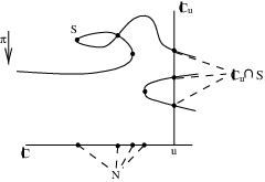
In order to find the fundamental group $\pi_{1}({\mathbb{P}}^{2}\backslash{\mathcal{A}}_{n})$, we need the algorithm of Moishezon-Teicher for the global braid monodromy. Consider the following setting (Figure 5). $S$ is an algebraic curve in ${\mathbb{C}}^{2}$, with $p=\deg(S)$. Let $\pi:{\mathbb{C}}^{2}\rightarrow{\mathbb{C}}$ be a generic projection on the first coordinate. Define the fiber $K(x)=\{y\mid(x,y)\in S\}$ in $S$ over a fixed point $x$, projected to the $y$-axis. Define $N=\{x\mid\#K(x)<p\}$ and $M^{\prime}=\{s\in S\mid\pi_{\mid s}\mbox{ is not \'{e}tale at }s\}$; note that $\pi(M^{\prime})=N$. Let $\{A_{j}\}^{q}_{j=1}$ be the set of points of $M^{\prime}$ and $N=\{x_{j}\}^{q}_{j=1}$ their projection on the $x$-axis. Recall that $\pi$ is generic, so we assume that $\#(\pi^{-1}(x)\cap M^{\prime})=1$ for every $x\in N$. Let $E$ (resp. $D$) be a closed disk on the $x$-axis (resp. the $y$-axis), such that $M^{\prime}\subset E\times D$ and $N\subset\mbox{Int}(E)$. We choose $u\in\partial E$ a real point far enough from the set $N$, $x<<u$ for every $x\in N$. Define ${\mathbb{C}}_{u}=\pi^{-1}(u)$ and number the points of $K={\mathbb{C}}_{u}\cap S$ as $\{1,\dots,p\}$.

We construct a g-base for the fundamental group $\pi_{1}(E-N,u)$. Take a set of paths $\{\gamma_{j}\}^{q}_{j=1}$ which connect $u$ with the points $\{x_{j}\}^{q}_{j=1}$ of $N$. Now encircle each $x_{j}$ with a small oriented counterclockwise circle $c_{j}$. Denote the path segment from $u$ to the boundary of this circle as $\gamma^{\prime}_{j}$. We define an element (a loop) in the g-base as $\delta_{j}={\gamma^{\prime}}_{j}c_{j}{\gamma^{\prime}}^{-1}_{j}$. Let $B_{p}[D,K]$ be the braid group, and let $H_{1},\dots,H_{p-1}$ be its frame (for complete definitions, see [11, Section III.2]). The braid monodromy of $S$ [4] is a map $\varphi:\pi_{1}(E-N,u)\rightarrow B_{p}[D,K]$ defined as follows: every loop in $E-N$ starting at $u$ has liftings to a system of $p$ paths in $(E-N)\times D$ starting at each point of $K=1,\ldots,p$. Projecting them to $D$ we get $p$ paths in $D$ defining a motion $\{1(t),\dots,p(t)\}$ (for $0\leq t\leq 1$) of $p$ points in $D$ starting and ending at $K$. This motion defines a braid in $B_{p}[D,K]$. By the Artin Theorem [12], for $j=1,\dots,q$, there exists a halftwist $Z_{j}\in B_{p}[D,K]$ and $\epsilon_{j}\in{\mathbb{Z}}$, such that $\varphi(\delta_{j})=Z_{j}^{\epsilon_{j}}$, where $Z_{j}$ is a halftwist and $\epsilon_{j}=1,2$ or $4$ (for an ordinary branch point, a node, or a tangency point respectively). We explain now how to get this $Z_{j}$.

We explain how to get the braid monodromy around each singularity in $S$. Let $A_{j}$ be a singularity in $S$ and its projection by $\pi$ to the $x$-axis is $x_{j}$. We choose a point $x^{\prime}_{j}$ next to $x_{j}$, such that $\pi^{-1}(x^{\prime}_{j})$ is a typical fiber. We encircle $A_{j}$ with a very small circle in a way that the typical fiber $\pi^{-1}(x^{\prime}_{j})$ intersects the circle in two points, say $a,b$. We fix a skeleton $\xi_{x^{\prime}_{j}}$ which connects $a$ and $b$, and denote it as $<a,b>$. The Lefschetz diffeomorphism $\Psi$ (see [11]) allows us to get a resulting skeleton $(\xi_{x^{\prime}_{j}})\Psi$ in the typical fiber ${\mathbb{C}}_{u}$. This one defines a motion of its two endpoints. This motion induces a halftwist $Z_{j}=\Delta<(\xi_{x^{\prime}_{j}})\Psi>$. As above, $\varphi(\delta_{j})=\Delta<(\xi_{x^{\prime}_{j}})\Psi>^{\epsilon_{j}}$. The braid monodromy factorization associated to $S$ is $\Delta^{2}_{p}=\prod\limits^{q}_{j=1}\varphi(\delta_{j})$.

Before proving Theorem 5, we have to study the local monodromy around a common tangency point (of $n$ quadrics) and the relation which is derived from this monodromy. This is done in the following propositions.

We want to compute the braid monodromy factorization of ${\mathcal{A}}_{2}$. Consider the above general setting (see Figure 5). Let $K=\{1,2,3,4\}$ and let $\{j\}^{3}_{j=1}$ be singular points of $\pi_{1}$ on the right side of the chosen typical fiber as follows: $1$ is a tangency point, $2$ and $3$ are branch points of the quadrics.

We are looking for $\varphi(\delta_{j})$ for $j=1,2,3$. So we choose a $g$-base $\{\delta_{j}\}^{3}_{j=1}$ of $\pi_{1}(E-N,u)$, such that each $\delta_{j}$ is constructed from a path $\gamma_{j}$ below the real line and a counterclockwise small circle around the points in $N$.

The diffeomorphisms which are induced from passing through branch points were defined in [12] as $\Delta^{\frac{1}{2}}_{I_{2}{\mathbb{R}}}<k>$ and $\Delta^{\frac{1}{2}}_{I_{4}I_{2}}<k>$. We recall the precise definition from [12]. Consider a typical fiber on the left side of a branch point (locally defined by $y^{2}-x=0$). The typical fiber intersects the quadric in two complex points. Passing through this point, the two complex points move to the k’th place and rotate in a counterclockwise $90^{o}$ twist. They become real and numbered as $k,k+1$.

Find first the skeleton $\xi_{x^{\prime}_{j}}$ related to each singular point. Then compute the local diffeomorphisms $\delta_{j}$ induced from singular points $j$. The monodromy table is:

$j$	$\xi_{x^{\prime}_{j}}$	$\epsilon_{j}$	$\delta_{j}$
1	$<3,4>$	4	$\Delta^{2}<3,4>$
2	$<2,3>$	1	$\Delta^{\frac{1}{2}}_{I_{2}{\mathbb{R}}}<2>$
3	$<1,2>$	1	$\Delta^{\frac{1}{2}}_{I_{4}I_{2}}<1>$

Using [12], we compute the skeleton $(\xi_{x^{\prime}_{j}})\Psi_{\gamma^{\prime}_{j}}$ to each $j$ by applying to the skeleton $\xi_{x^{\prime}_{j}}$ the product $\prod\limits_{i=j-1}^{1}\delta_{i}$.

• $(\xi_{x^{\prime}_{1}})\Psi_{\gamma^{\prime}_{1}}=<3,4>=z_{3\ 4}$
  $\varphi(\delta_{1})=Z^{4}_{3\ 4}$

  

• $(\xi_{x^{\prime}_{2}})\Psi_{\gamma^{\prime}_{2}}=<2,3>\Delta^{2}<3,4>=z_{2\ 3}^{Z^{2}_{3\ 4}}$
  $\varphi(\delta_{2})={Z_{2\ 3}}^{Z^{2}_{3\ 4}}$

  

• $(\xi_{x^{\prime}_{3}})\Psi_{\gamma^{\prime}_{3}}=<1,2>\Delta^{\frac{1}{2}}_{I_{2}{\mathbb{R}}}<2>\Delta^{2}<3,4>={z}_{1\ 4}$
  $\varphi(\delta_{3})={Z}_{1\ 4}$

  

On the left side of the typical fiber (Figure 8) we have three singularities and the related monodromy table is:

$j$	$\xi_{x^{\prime}_{j}}$	$\epsilon_{j}$	$\delta_{j}$
1	$<1,2>$	4	$\Delta^{2}<1,2>$
2	$<2,3>$	1	$\Delta^{\frac{1}{2}}_{I_{2}{\mathbb{R}}}<2>$
3	$<1,2>$	1	$\Delta^{\frac{1}{2}}_{I_{4}I_{2}}<1>$

And again by the Moishezon-Teicher algorithm [12] we have the following resulting braids:

• $(\xi_{x^{\prime}_{1}})\Psi_{\gamma^{\prime}_{1}}=<1,2>=z_{1\ 2}$
  $\varphi(\delta_{1})=Z^{4}_{1\ 2}$

  

• $(\xi_{x^{\prime}_{2}})\Psi_{\gamma^{\prime}_{2}}=<2,3>\Delta^{2}<1,2>=z_{2\ 3}^{Z^{2}_{1\ 2}}$
  $\varphi(\delta_{2})={Z_{2\ 3}}^{Z^{2}_{1\ 2}}$

  

• $(\xi_{x^{\prime}_{3}})\Psi_{\gamma^{\prime}_{3}}=<1,2>\Delta^{\frac{1}{2}}_{I_{2}{\mathbb{R}}}<2>\Delta^{2}<1,2>=\bar{z}_{1\ 4}$
  $\varphi(\delta_{3})=\bar{Z}_{1\ 4}$

  

According to the van Kampen Theorem [18], we get the following set of relations for $\pi_{1}({\mathbb{P}}^{2}\backslash{\mathcal{A}}_{2})$:

	$\displaystyle(34)^{2}=(43)^{2}$
	$\displaystyle 2=434^{-1}$
	$\displaystyle 1=4$
	$\displaystyle(12)^{2}=(21)^{2}$
	$\displaystyle 3=2121^{-1}2^{-1}$
	$\displaystyle 4=3212^{-1}3^{-1}$
	$\displaystyle 4321=e\ \ \mbox{(the projective relation).}$

By an easy simplification, we get $\pi_{1}({\mathbb{P}}^{2}\backslash{\mathcal{A}}_{2})\simeq\langle a_{1},a_{2}\left|(a_{1}a_{2})^{2}=e\right\rangle$.

Now we consider the arrangement ${\mathcal{A}}_{3}$. In a similar way as done for ${\mathcal{A}}_{2}$, we compute the relevant monodromy and we are able to find out that $\pi_{1}({\mathbb{P}}^{2}\backslash{\mathcal{A}}_{3})\simeq\langle a_{1},a_{2},a_{3}\left|(a_{1}a_{2}a_{3})^{2}=e\right\rangle$.

In order to compute the group $\pi_{1}({\mathbb{P}}^{2}\backslash{\mathcal{A}}_{n})$, we have to apply again the Moishezon-Teicher algorithm for the global monodromy. On each one of the sides of the typical fiber in Figure 2 we have one tangency point and $n$ branch points. The relation related to a tangency point was proved in Proposition 12. Since we have two tangency points in the arrangement, we have relations (6) and (11). The relations relating to the right branch points are (7)- -(10), and the relations relating to the left branch points are (12)- -(15):

(6)		$\displaystyle(a_{n+1}a_{n+2}\cdots a_{2n})^{2}=(a_{2n}a_{n+1}\cdots a_{2n-1})^{2}=\dots=(a_{n+2}a_{n+3}\cdots a_{2n}a_{n+1})^{2}$
(7)		$\displaystyle a_{n}=a_{2n}a_{2n-1}\cdots a_{n+2}a_{n+1}a_{n+2}^{-1}\cdots a_{2n-1}^{-1}a_{2n}^{-1}$
(8)		$\displaystyle a_{n-1}=a_{2n}a_{2n-1}\cdots a_{n+3}a_{n+2}a_{n+3}^{-1}\cdots a_{2n-1}^{-1}a_{2n}^{-1}$
(9)		$\displaystyle a_{n-2}=a_{2n}a_{2n-1}\cdots a_{n+4}a_{n+3}a_{n+4}^{-1}\cdots a_{2n-1}^{-1}a_{2n}^{-1}$
	$\displaystyle\dots\dots$
(10)		$\displaystyle a_{1}=a_{2n}$
(11)		$\displaystyle(a_{1}a_{2}\cdots a_{n})^{2}=(a_{n}a_{1}\cdots a_{n-1})^{2}=\dots=(a_{2}a_{3}\cdots a_{n}a_{1})^{2}$
(12)		$\displaystyle a_{n+1}=a_{n}a_{n-1}\cdots a_{1}a_{n}a_{1}^{-1}\cdots a_{n-1}^{-1}a_{n}^{-1}$
(13)		$\displaystyle a_{n+2}=a_{n+1}a_{n}\cdots a_{1}a_{n-1}a_{1}^{-1}\cdots a_{n}^{-1}a_{n+1}^{-1}$
(14)		$\displaystyle a_{n+3}=a_{n+2}a_{n+1}\cdots a_{1}a_{n-2}a_{1}^{-1}\cdots a_{n+1}^{-1}a_{n+2}^{-1}$
	$\displaystyle\dots\dots$
(15)		$\displaystyle a_{2n}=a_{2n-1}a_{2n-2}\cdots a_{2}a_{1}a_{2}^{-1}\cdots a_{2n-2}^{-1}a_{2n-1}^{-1}$
(16)		$\displaystyle a_{2n}a_{2n-1}a_{2n-2}\cdots a_{2}a_{1}=e\ \ \mbox{(the projective relation).}.$

We substitute relations (7)- -(10) in relations (12)- -(15) and get for each one of them one of the following equations:

$$(a_{n+1}a_{n+2}\cdots a_{2n})^{-2}=(a_{2n}a_{n+1}\cdots a_{2n-1})^{-2}=\dots=(a_{n+2}a_{n+3}\cdots a_{2n}a_{n+1})^{-2}.$$

These equations appear already in (6). Therefore relations (12)- -(15) are redundant.

Also relation (11) gets the same form of (6), again by substituting relations (7)- -(10), and therefore it is redundant too.

By the same substitution, relation (16) is rewritten as $(a_{n+1}a_{n+2}\cdots a_{2n})^{2}=~e$. Hence, we get the presentation (3), as needed. $\Box$

The arrangement ${\mathcal{B}}_{n}$ is depicted in Figure 3. We start with ${\mathcal{B}}_{1}$ (a smooth quadric), and it is easy to see that the group $\pi_{1}({\mathbb{P}}^{2}\backslash{\mathcal{B}}_{1})$ is ${\mathbb{Z}}_{2}$. Now we compute the braid monodromy factorization of the curve ${\mathcal{B}}_{2}$. We follow Figure 9.

Let $\pi_{1}:E\times D\rightarrow E$ be the projection to $E$. Take $u\in\partial E$, such that ${\mathbb{C}}_{u}$ is a typical fiber and $M\in{\mathbb{C}}_{u}$ is a real point. Let $K=K(M)=\{1,2,3,4\}$. Let $\{j\}^{3}_{j=1}$ be singular points of $\pi_{1}$ on the right side of the chosen typical fiber as follows: $1$ is a tangency point, $2$ and $3$ are branch points of the quadrics. Let $N=\{x(j)=x_{j}\mid 1\leq j\leq 3\}$, such that $N\subset E-\partial E,N\subset E$. We start with the monodromy table:

$j$	$\xi_{x^{\prime}_{j}}$	$\epsilon_{j}$	$\delta_{j}$
1	$<3,4>$	8	$\Delta^{4}<3,4>$
2	$<2,3>$	1	$\Delta^{\frac{1}{2}}_{I_{2}{\mathbb{R}}}<2>$
3	$<1,2>$	1	$\Delta^{\frac{1}{2}}_{I_{4}I_{2}}<1>$

By the algorithm from [12], we compute the monodromies:

• $(\xi_{x^{\prime}_{1}})\Psi_{\gamma^{\prime}_{1}}=<3,4>=z_{3\ 4}$
  $\varphi(\delta_{1})=Z^{8}_{3\ 4}$

  

• $(\xi_{x^{\prime}_{2}})\Psi_{\gamma^{\prime}_{2}}=<2,3>\Delta^{4}<3,4>=z_{2\ 3}^{Z^{4}_{3\ 4}}$
  $\varphi(\delta_{2})={Z_{2\ 3}}^{Z^{4}_{3\ 4}}$

  

• $(\xi_{x^{\prime}_{3}})\Psi_{\gamma^{\prime}_{3}}=<1,2>\Delta^{\frac{1}{2}}_{I_{2}{\mathbb{R}}}<2>\Delta^{4}<3,4>={z}_{1\ 4}^{Z^{2}_{3\ 4}}$
  $\varphi(\delta_{3})={{Z}_{1\ 4}}^{Z^{2}_{3\ 4}}$

  

On the left side of the typical fiber in Figure 9 we have two branch points and the related monodromy table is:

$j$	$\xi_{x^{\prime}_{j}}$	$\epsilon_{j}$	$\delta_{j}$
1	$<2,3>$	1	$\Delta^{\frac{1}{2}}_{I_{2}{\mathbb{R}}}<2>$
2	$<1,2>$	1	$\Delta^{\frac{1}{2}}_{I_{4}I_{2}}<1>$

And we have the following resulting braids:

• $(\xi_{x^{\prime}_{1}})\Psi_{\gamma^{\prime}_{1}}=<2,3>=z_{2\ 3}$
  $\varphi(\delta_{1})=Z_{2\ 3}$

  

• $(\xi_{x^{\prime}_{2}})\Psi_{\gamma^{\prime}_{2}}=<1,2>\Delta^{\frac{1}{2}}_{I_{2}{\mathbb{R}}}<2>=z_{1\ 4}^{Z^{2}_{1\ 3}}$
  $\varphi(\delta_{2})={Z_{1\ 4}}^{Z^{2}_{1\ 3}}$

  

The relations which are related to these braids are as follows:

	$\displaystyle(34)^{4}=(43)^{4}$
	$\displaystyle 2=43434^{-1}3^{-1}4^{-1}$
	$\displaystyle 1=4343^{-1}4^{-1}$
	$\displaystyle 2=3$
	$\displaystyle 1=3^{-1}43$
	$\displaystyle 4321=e\ \ \mbox{(the projective relation)}.$

By an easy simplification, we get $\pi_{1}({\mathbb{P}}^{2}\backslash{\mathcal{B}}_{2})\simeq\langle a_{1},a_{2}\left|(a_{1}a_{2})^{2}=e\right\rangle$.

References

• [1] Amram, M.: Braid group and braid monodromy, M.Sc. Thesis, Bar-Ilan University, (1995).
• [2] Amram, M., Teicher, M.: Braid monodromy of special curves, Journal of Knot Theory and its Ramifications 10 (2001), no. 2, 171-212.
• [3] Amram, M., Garber, D., Teicher, M.: Fundamental groups of tangented conic-line arrangements with singularities up to order 66, Mathematische Zeitschrift, http://dx.doi.org/10.1007/s00209-007-0109-4.
• [4] Artin, E., Theory of braids, The Annals of Mathematics 48 (1947), 101-126.
• [5] Cheniot, D.: Topologie du complémentaire d’un ensemble algébrique projectif, Enseign. Math., II. Sér. 37 (1991), no.3/4, 293-402.
• [6] Dimca, A.: Singularities and the topology of hypersurface complements, Universitext. New York etc.: Springer-Verlag (1992).
• [7] Garber, D., Teicher, M.: The fundamental group’s structure of the complement of some configurations of real line arrangements, Complex Analysis and Algebraic Geometry. A volume in memory of Michael Schneider, Berlin: Walter de Gruyter (2000), 173-223.
• [8] Hartshorne, R.: Algebraic Geometry, Graduate Texts for Mathematics, Springer (1977).
• [9] Holzapfel, R.P., Vladov. N.: Quadric-line configurations degenerating plane Picard-Einstein metrics I-II, Sitzungsberichte der Berliner Mathematischen Gesellschaft, Berliner Math. Gesellschaft, Berlin (2001), 79-141.
• [10] Lamotke, K.: The topology of complex projective varieties after S. Leftschez, Topology 20 (1979), 15-51.
• [11] Moishezon, B., Teicher, M., Braid group technique in complex geometry I, Line arrangements in ℂ​ℙ2{\mathbb{C}}{\mathbb{P}}^{2}, Contemporary Math. 78 (1988), 425-555.
• [12] Moishezon, B., Teicher, M.: Braid group techniques in complex geometry II, From arrangements of lines and conics to cuspidal curves, Algebraic Geometry, Lect. Notes in Math. 1479 (1990), 131-180.
• [13] Orlik, P., Salomon, L.: Arrangements defined by unitary reflection groups, Math. Ann. 261 (1982), 339-357.
• [14] Orlik, P., Terao, H.: Arrangements of Hyperplanes, Grundlagen der matematichen Wissenshaften 300, Berlin, Springer-Verlag (1992).
• [15] Suciu, A.: Fundamental groups of line arrangements: Enumerative aspects, Contemp. Math. 276 (2001), 43-79.
• [16] Uludağ, A.M.: On finite smooth uniformizations of the plane along line arrangements, in preparation.
• [17] Uludağ, A.M.: Covering relations between ball quotient orbifolds, Math. Ann. 328 (2004), no.3, 503-523.
• [18] van Kampen, E.R.: On the fundamental group of an algebraic curve, Amer. J. Math. 55 (1933), 255-260.
• [19] Kaneko, J., Tokunaga, S., Yoshida, M.: Complex crystallographic groups II, J. Math. Soc. Japan 34 (1982), no. 4.