The blocks of the Brauer algebra
in characteristic zero
Abstract.
We determine the blocks of the Brauer algebra in characteristic zero. We also give information on the submodule structure of standard modules for this algebra.
2000 Mathematics Subject Classification
Primary 20G051. Introduction
The Brauer algebra was introduced in [Bra37] in the study of the representation theory of orthogonal and sympletic groups. Over , and for integral values of , its action on tensor space can be identified with the centraliser algebra for the corresponding group action. This generalises the Schur-Weyl duality between symmetric and general linear groups [Wey46].
If is fixed, then for all the centraliser algebra has multimatrix structure independent of , and Brauer’s algebra unifies these algebras, having a basis independent of , and a composition which makes sense over any field and for any . The Brauer algebra is well defined in particular for positive integral , but the action on is faithful for positive integral if and only if .
In classical invariant theory one is interested in the Brauer algebra per se only in so far as it coincides with the centraliser of the classical group action on ; i.e., in the case of integral with large compared to . Here we take another view, and consider the stable properties for fixed and arbitrarily large . In such cases is not semisimple for integral. However it belongs to a remarkable family of algebras arising both in invariant theory and in statistical mechanics for which this view is very natural. (For example when considered from the point of view of transfer matrix algebras in statistical mechanics [Mar91].) Indeed much of the structure of can be recovered from a suitable global limit of by localisation (and in this sense its structure does not depend on ).
This family of algebras can be introduced as follows. Consider the diagram of commuting actions on , with :
where the actions of the algebra on the right centralise the action of the group on the left in the same row, and vice versa. The bottom row consists of the diagonal action of permuting the standard ordered basis of on the left, and the partition algebra on the right. The partition algebra (for any ) has a basis of partitions of two rows of vertices. The Brauer algebra is the subalgebra with basis the subset of pair partitions, and is the subalgebra with basis the pair partitions such that each pair contains a vertex from each row. The Brauer algebra also has a subalgebra with basis the set of pair partitions which can be represented by noncrossing lines drawn vertex-to-vertex in an interval of the plane with the rows of vertices on its boundary. This is the Temperley-Lieb algebra .
All of these algebras are rather well understood over , with the exception of . All their decomposition matrices are known, and all of their blocks can be described by an appropriate geometric linkage principle. For both data are trivial, since it is semisimple. For each standard module has either one or two composition factors and its alcove geometry is affine (affine reflections on the real line). For each standard module has either one or two composition factors and its alcove geometry is affine (although locally the block structure looks like affine ).
Over , the Brauer algebra is semisimple for sufficiently large, and is generically semisimple [Bro55]. Hanlon and Wales studied these algebras in a series of papers [HW89b, HW89a, HW90, HW94] and conjectured that is semi-simple for all non-integral choices of . This was proved by Wenzl [Wen88].
In this paper we determine the blocks of for integral. The simple modules of may be indexed by partitions of those natural numbers congruent to modulo 2 and not exceeding , and hence by Young diagrams (if then the empty partition is omitted). We will call these indexing objects weights. Given a ring we can associate a charge to each box in a Young diagram, as shown in Figure 1. We will also refer later to the usual content of boxes which, for the box in -th row and -th column is . It is easy to see that . For each pair of diagrams and we will also need to consider the skew partitions and consisting of those boxes occuring in but not and in but not .
With these notations we can now state the two main results of the paper (which are valid without restriction on ).
Corollary 6.7.
The simple modules and are in the same block if and only if
(i) The boxes in (respectively ) can be put into pairs whose charges sum to zero;
(ii) if (respectively contains with no to the right of these boxes then it contains an even number of 1/-1 pairs.
Examples illustrating this result are given in Example 4.9.
Theorem 7.3 (Summary).
For any integral and natural number a standard module can be constructed (for some ) whose socle series length is greater than . This module also has a socle layer containing at least simples.
The second result shows that the structure of standard modules can become arbitrarily complicated. This is in marked contrast to the partition and Temperley-Lieb algebra, and symmetric group, cases.
To prove these results we use the theory of towers of recollement developed in [CMPX]. This approach is already closely modelled, for , in work of Doran, Wales, and Hanlon [DWH99] (since both papers use the methods developed in [Mar96]). This key paper of Doran, Wales and Hanlon will be the starting point for our work, and we will generalise and refine several of their results.
The ‘diagram’ algebras are amenable to many powerful representation theory techniques, and yet the representation theory of the Brauer algebra is highly non-trivial in comparison to the others. We shall see that, in terms of degree of difficulty, the study of Brauer representation theory in characteristic zero is an intermediate between the study of ‘classical’ objects in characteristic zero and the grand theme of the representation theory of finite dimensional algebras, the study of in characteristic .
Another such intermediate class of objects are the Hecke algebras of type at roots of unity, which are Ringel dual to the generalised Lie objects known as quantum groups. The Brauer algebra in characteristic zero has, through its global limit, more Lie-theory-like structure than in characteristic (for which not even a good organisational scheme within which to address the problem is known, for small primes ). This is reminiscent of the virtual algebraic Lie theory discussed for the (generalised) blob algebras in [MRH04, MW03]. However in the Brauer algebra case, any candidate for an alcove geometry formulation will be considerably more complicated [Naz96, OR01]. For these reasons we consider the further study of the Brauer algebra in characteristic zero to be an important problem in representation theory.
The paper begins with a section defining the various objects of interest, and a review of their basic properties in the spirit of [CMPX]. This is followed by a brief section describing some basic results about Littlewood-Richardson coefficients which will be needed in what follows. In Section 4 we begin the analysis of blocks by giving a necessary condition for two weights to be in the same block. This is based on an analysis of the action of certain central elements in the algebra on standard modules, and inductive arguments using Frobenius reciprocity. Section 5 constructs homomorphisms between standard modules in certain special cases, generalising a result in [DWH99]. Although not necessary for the main block result, this is of independent interest.
The classification of blocks is completed in Section 6. The main idea is to show that every block contains a unique minimal weight, and that there is a homomorphism from any standard labelled by a non-minimal weight to one labelled by a smaller weight. We also describe precisely which weights are minimal in their blocks.
In Section 7 we consider certain explicit choice of weights, and show inductively, via Frobenius reciprocity arguments, that the corresponding standards can have arbitrarily complicated submodule structures. We conclude by outlining the modifications to our arguments required in the case .
The structure of the Brauer algebra becomes mouch more complicated when considered over an arbitrary field . For general and integral it is expected that this algebra still acts as a centraliser algebra, and this has been shown in a recent series of papers for the symplectic case [Dot98, Oeh01, DDH]. A necessary and sufficient condition for semisimplicity (which holds over arbitrary fields) was given recently by Rui [Rui05]. The study of Young and permutation modules for these algebras has been started in [HP].
2. Preliminaries
In this section we will consider the Brauer algebra defined over a general field of characteristic , although we will later restrict attention to the case . After reviewing the definition of the Brauer algebra, we will show that families of such algebras form towers of recollement in the sense of [CMPX] (which we will see follows from various results of Doran et. al. [DWH99]). This will be the framework in which we base our analysis of these algebras.
Given and , the Brauer algebra is a finite dimensional associative -algebra generated by certain Brauer diagrams. A general -(Brauer) diagram consists of a rectangular box (or frame) with distinguished points on the northern boundary and distinguished points on the southern boundary, which we call nodes. Each node is joined to precisely one other by a line, and there may also be one or more closed loops inside the frame. Those diagrams without closed loops are called reduced. We will label the northern nodes from left to right by and the southern nodes from left to right by . We identify diagrams if they connect the same pairs of labelled nodes, and have the same number of closed loops. Lines which connect two nodes on the northern (respectively southern) boundary will be called northern (respectively southern) arcs; those connecting a northern node to a southern node will be called propagating lines.

Given an -diagram and a -diagram , we define the product to be the -diagram obtained by concatenation of above (where we identify the southern nodes of with the northern nodes of and then ignore the section of the frame common to both diagrams). As a set, the Brauer algebra consists of linear combinations of -diagrams. This has an obvious additive structure, and multiplication is induced by concatenation. We also impose the relation that any non-reduced diagram containing closed loops equals times the same diagram with all closed loops removed. A basis is then given by the set of reduced diagrams. An example of a product of two diagrams in given in Figure 2. For convenience, we set . When no confusion is likely to arise, we denote the algebra simply by .
We will now apply as much as possible from the general setup of [CMPX] to the Brauer algebra. The labels (A1), (A2), etc., refer to the axioms in that paper. Henceforth, we assume that ; for the case see Section 8.
For consider the idempotent in defined by times the Brauer diagram where is joined to for , and is joined to and is joined to . This is illustrated in Figure 3.

Lemma 2.1 (A1).
For each , we have an algebra isomorphism
which takes a diagram in to the diagram in obtained by adding an extra northern and southern arc to the righthand end.
This allows us to define, following Green [Gre80], an exact localization functor
and a right exact globalization functor
Note that for all , and hence is a full embedding.
From this we can quickly deduce an indexing set for the isomorphism classes of simple -modules. It is easy to see that
| (1) |
the group algebra of the symmetric group on symbols. If the simple -modules are indexed by the set then by [Gre80] and Lemma 2.1, the simple -modules are indexed by the set
where or depending on the parity of . If or then the set corresponds to the set of partitions of ; we write if is such a partition.
For even we write for regarded as a subset of . (If then .) We also write for the disjoint union of all the , and call this the set of weights for the Brauer algebra. We will henceforth abuse terminology and refer to weights as being in the same block of if the corresponding simple modules are in the same block.
For and , define the idempotent to be if or times the Brauer diagram with edges between and for all and between and , and and for . (This is the image of via the isomorphisms arising in Lemma 2.1.) Set .
Lemma 2.2 (A2).
The natural multiplication map
is bijective. If and either or then is semisimple.
Proof.
The second part follows from (1) and standard
symmetric group results. For the first part, the map is clearly
surjective so we only need to show that it is also injective. It is
easy to verify that:
(i) has a basis given by all reduced
diagrams having at least propagating lines,
(ii)
has a basis given by all reduced diagrams
having exactly vertical edges, and
(iii)
.
Now suppose that and are diagrams in . Any such diagram has a southern edge where the leftmost nodes lie on propagating lines, with the remaining southern nodes paired consecutively. The northern edge has exactly northern arcs. We will label such a diagram by , where represents the configuration of northern arcs, represents the fixed southern boundary, and is the permutation obtained by setting if the th propagating northern node from the left is connected to . (For later use we will denote the set of elements arising thus by , and call such elements partial one-row diagrams.) Similarly a diagram in will be labelled by .
It will be enough to show that the multiplication map is injective on the set of tensor products of diagram elements. Given and in and , in , assume that . Then we must have , and . It now follows from the identifcation in (iii) that in . ∎
We immediately obtain
Corollary 2.3 (A2′).
If and either or then is a quasi-hereditary algebra, with heredity chain given by
The partial ordering is given as follows: for we have if and only if either or and with .
Henceforth we assume that satisfies the conditions in Corollary 2.3. It follows from the quasi-hereditary structure that for each we have a standard module having simple head and all other composition factor satisfying . Note that if then
the lift to of the Specht module for .
Note also that by [Don98, A1] and arguments as in [MRH04, Proposition 3], the quasi-hereditary structure is compatible with the globalization and localization functors. That is, for all we have
| (2) | |||
As is exact we also have that
For every partition of some we can give an explicit construction of the modules . Let be as above, so that . If we denote by the lift of the Specht module labelled by for to , then by (2) we have that
| (9) |
Using this fact, it is easy to give a basis for this module in terms of some basis of , using the notation introduced during the proof of Lemma 2.2.
Lemma 2.4.
If is a partition of then the module has a basis given by
Via this Lemma we may identify our standard modules with the modules in [DWH99] (which in turn come from [Bro55]). Note that if we define as the tensor product in (9) then we have a definition that makes sense for all values of . In the non-quasi-hereditary cases these modules still play an important role, as the algebras are cellular [GL96] with the as cell modules.
We will frequently need a second way to relate different Brauer algebras.
Lemma 2.5 (A3).
For each , the algebra can be identified as a subalgebra of via the homomorphism which takes a Brauer diagram in to the Brauer diagram in obtained by adding two vertices and with a line between them.
We can relate these functors to globalisation and localisation via
Lemma 2.6 (A4).
(i) For all we have that
as a left , right
-bimodule.
(ii) For all -modules
we have
Proof.
(i) Every Brauer diagram in has an edge between
and . Define a map from to
by sending a diagram to the diagram with
vertices obtained from by removing the line connecting
and and and the line from , and pairing
the vertex to the vertex originally paired with
in . It is easy to check that this gives an isomorphism.
(ii) Using (i) we have
∎
Let be a partition of and be a partition of . We write and if is obtained from by removing a box from its Young diagram (equivalently if is obtained from by adding a box to its Young diagram). The following result does not require any restriction on the characteristic of our field.
Proposition 2.7 (A5 and 6).
For we have short exact sequences
and
Proof.
Wenzl [Wen88] has shown that is semisimple when and . (Over an arbitrary field, a necessary and sufficient condition for semisimplicity has been given by Rui [Rui05].) For this reason we do not consider the case of non-integral . As we will regularly need to appeal to the representation theory of the symmetric group, which is not well understood in positive characteristic, we will also only consider the characteristic zero case. In summary:
Henceforth we will assume that and , unless otherwise stated.
3. Some Littlewood-Richardson coefficients
One of the key results used by [DWH99] in their analysis of the Brauer algebra is [HW90, Theorem 4.1] which decomposes standard modules with as symmetric group modules. Recall that a partition is even if every part of the partition is even, and that denotes a Littlewood-Richardson coefficient. If and then [HW90, Theorem 4.1] states that either or for some and
| (10) |
As this result is stated in terms of Littlewood-Richardson coefficients, we will find it useful to calculate these in certain special cases.
Lemma 3.1.
If are partitions such that is also a partition then
Proof.
This follows immediately from the definition of Littlewood-Richardson coefficients in terms of rectification of skew tableaux (see [Ful97, Section 5.1, Corollary 2]) ∎
For our second calculation we will need an alternative definition of
Littlewood-Richardson coefficients (which can be found in [JK81, 2.8.14
Corollary]). When considering a configuration of boxes labeled by
elements we say that the configuration is valid if:
(i) For all , if then
is in a later column than .
(ii)
For all , if then is in an earlier row than
.
For each box of consider a symbol
. Then the Littlewood-Richardson coefficient is the number of ways one can form from
by adding the boxes of to in the following manner. First
add to to form a new
partition . Continue inductively by adding
to to form a new
partition . We require that the final configuration of the
elements is valid.
Lemma 3.2.
If are partitions with for some and then there is a unique partition such that , and for this partition we have . Further, .
Proof.
Consider valid extensions of by any to form . As is a rectangle, the final row of can only be placed as illustrated in Figure 4(a). Then the penultimate row of must be placed as illustrated in Figure 4(b). Continuing in this way we see that the choice of is unique, and the number of boxes in the final row of must equal , in the penultimate row must equal , and so on. ∎
|
|
||||||||||||||||||
4. A partial block result
Doran, Wales, and Hanlon [DWH99] have given a necessary condition for the existence of a non-zero homomorphism of -modules from to . We will first elevate this condition to a partial block result, and then give a stronger necessary condition that must also hold for two weights to be in the same block. In section 6 we will see that this stronger condition is also sufficient for two weights to be in the same block.
Let be a partition. For a box in the corresponding Young diagram , we denote by the content of . Recall that if is in the -th row (counting from top to bottom) and in the -th column (counting from left to right) of , then . We denote by the multiset . If is a partition with we write , and denote the skew partition obtained by removing from by . We then denote by the multiset .
Write for the Brauer diagram in with edges between and for all and with edges between and and between and . Note that is generated by the elements together with the symmetric group (identified with the set of diagrams with propagating lines). We denote by the element in . Recall also the definition of partial one-row diagrams in the proof of Lemma 2.2.
Lemma 4.1.
Let be a partition of with . For all and we have that
where denotes the element of which transposes and . Hence for all we have
Proof.
The next result is a slight strengthening of [DWH99, Theorem 3.3] (which in turn generalises [Naz96, formula before (2.13)], which considers the case ). The original results provide a necessary condition for the existence of a homomorphism between two standard modules, but can be refined to prove
Proposition 4.2.
Suppose that . Then either or and for some . Further, we must have
Proof.
The first part of the proposition is clear from the quasi-hereditary structure of . For the second part, note that by using the exactness of the localization functor we have
and hence we may assume that is a partition of . In this case, , the lift of the Specht module for to , and so any Brauer diagram having fewer than propagating lines must act as zero on . In particular, all the ’s act as zero and hence so does .
The condition that now follows by regarding as a -module by restriction and using (10) which describes the multiplicities of composition factors of such a module.
For the final condition, we know by assumption that there must exist a -submodule of and a -homomorphism
Let be the -submodule of containing such that
As is semisimple, we can find a -submodule of such that and . By Lemma 4.1 we have for all that
But is a simple -module and is in the centre of , so it must act as a scalar on . It is well known [Dia, Chapter 1] that this scalar is given by . Hence we have
But must act as zero on and hence . ∎
By standard quasi-heredity arguments [Don98, Appendix] we deduce
Corollary 4.3.
Suppose that and with . If and are in the same block then for some and
| (11) |
When [DWH99] gave a necessary and sufficient condition for the existence of a standard module homomorphism. From their results we obtain
Theorem 4.4.
Proof.
It is enough to consider the case when , as the general case follows by globalisation. If and do not satisfy the required conditions then there is no composition factor in (and hence no homomorphism) by Corollary 4.3 and the remarks after [DWH99, Theorem 3.1]. In the remaining cases the existence of such a homomorphism was shown in [DWH99, Theorem 3.4]. By the remarks after [DWH99, Theorem 3.1] the multiplicity of the simple module in is , and the dimension result is now immediate. ∎
The next result is a strengthening of Proposition 4.2.
Proposition 4.5.
Suppose that . Then there is a pairing of the boxes in such that the sum of the content of the boxes in each pair is equal to .
Proof.
We use induction on ; the case is covered by Proposition 4.2. Thus we assume that the result holds for and will show that it holds for .
If then by Proposition 4.2 we know that and
| (12) |
where . Now suppose, for a contradiction, that there is no pairing of the boxes of satisfying the condition of the proposition. By localising we may assume that is a partition of , so that . Thus has a submodule such that .
The partition has a removable box of content say and by Proposition 2.7 we have a surjection . Hence we have
and so by Frobenius reciprocity we have
This implies that
is a composition factor of . Now using
Proposition 2.7 we see that either
(i) the weight has a removable box such that
, or
(ii) the weight has an addable box such that
.
We consider each case in turn.
In case (i), Proposition 4.2 implies that and
Hence from (12) we must have
and by induction we can find a pairing of the boxes in such that the sum of the content of the boxes in each pair is equal to . But as multisets
and hence there is such a pairing for the boxes of . This gives the desired contradiction.
Now consider case (ii). Here has an addable box such that and
Comparing with (12) we deduce that
By induction there is a pairing of the boxes of satisfying the condition of the Proposition. But as multisets
and as observed above the and can be paired in the right way. Hence the boxes of can be paired appropriately, which again gives the desired contradiction. ∎
When is even we will need a further refinement of Proposition 4.2. Given , consider the boxes with content and in . If then these must be paired by Proposition 4.5, and so must be in one of the two chain configurations illustrated in Figure 5 (for some length of chain).

Proposition 4.6.
Suppose that and is even. If the boxes of content and are configured as in Figure 5(b) then the number of columns in this configuration must be even.
Proof.
We will show by induction on that in case (b) the number of columns must be even. The case is covered by Theorem 4.4.
By repeated applications of we may assume that . Let be a removable box of . As in the proof of Proposition 4.5 we have that if
then either
for some removable box of with and , or
for some addable box of with and .
If is not equal to either or then the boxes of (respectively of ) of content and are the same as those boxes in , and so the result follows by induction. Also, by our assumption on the configuration of such boxes the partition does not have a removable box of content . Thus we may assume that has only one removable box of content (and hence that is a rectangle).

We have that and are of the form shown in Figure 6, with . So in particular
By (10) we have
and hence we must have for some even partition . As is a rectangle Lemma 3.2 implies there is only one possible , and that each row of has length for some . But was an even partition and hence these lengths are all even, which implies that the number of columns occupied by shaded boxes in Figure 6 is also even as required. ∎
Definition 4.7.
We say that and are -balanced (or just balanced when the context is clear) if: (i) there exists a pairing of the boxes in (respectively in ) such that the contents of each pair sum to , and (ii) if is even and the boxes with content and in (respectively in ) are configured as in Figure 5(b), then the number of columns in this configuration is even.
Just as for Corollary 4.3 we can immediately deduce from Propositions 4.5 and 4.6 the following block result.
Corollary 4.8.
If and are in the same block then they are balanced.

Example 4.9.
(i) Let , , , and . The diagrams , , and are illustrated (with their contents) in Figure 7. Clearly
and hence
and satisfy the conditions in Corollary
4.3. However, there is no pairing of the boxes in such
that the content of each pair sums to zero, and hence and
cannot lie in the same block.
(ii) Let ,
, , and . The
diagrams , , and are illustrated (with
their contents) in Figure 7. In this case the boxes in
can be put into pairs such that each pair sums to
, but the boxes with contents and are in
configuration (b) from Figure 5, and occupy an odd number of columns. Hence and cannot lie in the same block.

By Corollary 4.8 weights which are not balanced will lie in different blocks. Hence for a -module we will denote by the direct summand of with composition factors such that and are balanced.
Lemma 4.10.
Suppose that and .
(i) There exists a -module and a short exact sequence
Here if is a balanced pair or if no such exists. In the former case the sequence is non-split.
(ii) If
then .
Proof.
(i) The existence of such a sequence, and the form of , follows from Proposition 2.7 and Corollary 4.8. To see that the sequence is non split, we proceed by induction on , the case where being clear. By Frobenius reciprocity we have
| (13) |
By (2) and Lemma 2.6(ii) the left-hand side equals
As is simple, we have by the induction hypothesis and Theorem 4.4 that this Hom-space is one dimensional. Hence the right-hand side of (13) is also one dimensional, which by another application of Theorem 4.4 implies that the desired sequence is non-split as required.
Part (ii) is an immediate consequence of (i). ∎
5. Computing some composition multiplicities
So far we have concentrated on conditions which imply that weights lie in different blocks of the algebra. In this section we will find certain pairs of weights which do lie in the same block, which we will demonstrate by determining certain composition factors of standard modules, and homomorphisms between such modules.
We first consider the special case where the skew partition is itself a partition. For such pairs we will be able to show precisely when is a composition factor of . We first give a necessary condition, in Proposition 5.1, which is a generalisation of [DWH99, Corollary 9.1] (the latter only considers the case and homomorphisms rather than composition factors).
Proposition 5.1.
Let are partitions such that is also a partition. If
then where is even and , where is the content of the top lefthand box of . Moreover, in this case we have
Proof.
As usual, by localisation we can assume that is a partition of . First suppose that . As is simply the lift of for , we have that
By (10) we have
Hence we see that must be an even partition, and by Lemma 3.1 that .
On the other hand, using Proposition 4.5 we know that there is a pairing of the boxes of such that the sum of the content of the boxes in each pair is equal to . Clearly we have a submodule of and an embedding
If is any removable box of then we have a surjective homomorphism
Composing these maps we see that
and so by Frobenius reciprocity we have
Thus
and hence either must have a removable box such that
or must have an addable box such that
In the first case we have and hence . However, as is a partition this is impossible, as no removable box in can have the same content as some box in . Hence we must be in the second case with , so in fact must be a box in . As is a partition, there is only one such addable box and its content is given by . Thus we must have
Now, if had another removable box then it would have to have the same content. But different removable boxes have different contents. Hence can only have one removable box, i. e. it is a rectangle , where is even as must be an even partition. The content of the only removable box of inside of is given by and this must be equal to . Hence we get
as required. ∎
We will show that the condition in Proposition 5.1 is also sufficient. This generalises [DWH99, Theorem 9.2], which again only considers homomorphisms and the case . Before doing this we will review some standard symmetric groups results which we will require. Details can be found in [Ful97, Chapter 7]
We will need to consider a set of idempotents in , such that . We will choose
| (14) |
where , is the column stabiliser of and is the row stabiliser of . For example and (regarded as elements of ) are illustrated in Figure 9.

We will also need the fact that
As all these group algebras are semisimple, this implies by Frobenius reciprocity that
| (15) |
Particular values of which we will need are those where , respectively . In these cases is at most , and is non-zero precisely when consists of two boxes in different columns, respectively different rows.
Theorem 5.2.
Supppose that and . If is even and where is the content of the top left box of then
Moreover, if then
Proof.
We can assume without loss of generality that . We have seen in the proof of Proposition 5.1 that . Let , which is isomorphic to as a -module. To show this is in fact a -submodule of , it will be enough to show that for all . Indeed, it is enough to show that this holds for a single choice of and , as
for all .
So let us fix and with and use the embedding
where is the symmetric group on and the symmetric group on . By (15) and the remarks following we have
where we sum over all ’s obtained from by removing 2 boxes in different rows and over all ’s obtained from by removing two boxes in different columns.
The map is a -homomorphism. Note that we have where is the span of all elements of the form where has an arc between and and . Regarding as a -module acting on the strings excluding and it is easy to see that is isomorphic to , and the restriction of this action to is the same as restriction to the action of the first component of regarded as a subalgebra of . Also, it is clear that kills the element in Figure 9, and hence kills the simple module . Combining these observations with (10) we deduce that, as a -module, decomposes as
where
Consider the restriction . We want to show that . Look at the simple summands of . Every summand of the form is sent to zero as it does not appear in . Moreover, if is not contained in then is sent to zero as only contains simple modules with . So we only need to show that
for any with and obtained from by removing two boxes in different columns. But there is only one such , namely the partition obtained from by removing two boxes from the last row of , i.e , and by Lemma 3.1 the coefficient of in equals .
Write where . As is simple, either embeds into or . Label the boxes of the partition with the numbers starting with the first row from left to right, then the second row from left to right, etc., until the last row. Say that the last box of the partition inside of is labelled by . Up until now was arbitrary; we now fix and and we want to show that .

Fix a partial one-row diagram with arcs defined as follows: suppose the -th row of inside of is labelled by for , as illustrated in Figure 10. Then is defined to have arcs for . (Note that .) We will represent elements of by adding bars to the Young tableau joining each pair of nodes connected by an arc. Thus the element will be represented by the diagram in Figure 11. Usually we will only represent the boxes of in such a diagram.
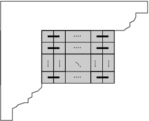
Now consider the element of given by for some . Then , so it decomposes as
where and . Note that this decomposition is independent of . As observed above, we have . Consider the coefficient of in . We will show that it is a non-zero multiple of
Hence, as is independent of we see that , but when , we have . Thus cannot embed into and so it must map to zero.
Using the labelling of the boxes of defined above, we will identify the row and column stabilisers and as subgroups of , the symmetric group on . From (14) we have
and so
We want to find the coefficient of in this sum. We consider several cases.
Case 1: Suppose that has an arc .
In this case . If we want to be in then we must have
where denotes the subgroup of (isomorphic to ) which preserves the rows of and fixes everything in and denotes the subgroup of which fixes as a diagram (i.e. fixes all but the northern arcs, which may be permuted amongst themselves and be reversed). In a similar way we define and .
Set . As the columns of are paired by the bars in , and each pair of such columns may be permuted freely by we have . Moreover as is an even permutation (as it is made up of pairs of identical permutations, corresponding to the paired ends of a bar) and so . Hence in this case we get the contribution
using for the second equality the isomorphisms and , and for the final equality the fact that for all .
Case 2: Suppose that neither nor is part of an arc in .
In this case has arcs in the top row and so .
Case 3: Suppose that in there are arcs and .
In this case, is obtained from by replacing the arcs and by the arcs and . Hence if we want to have lying in then must be an arc of and . Here we consider two subcases.
Subcase 3(a): First assume that the pair is not in the last double column. Then with and , where or such that is a box of in the same column as (possibly itself) and is the box of in the same row as and in the same column as . An example of such a situation is illustrated in Figure 12.

Thus we have choices for and choices for the position of (and hence of ), and so there are choices for . Hence there are choices for . Now where , and permutes the pairs in all double columns, except the last and the double column containing , arbitrarily. In the last double column it must send to and to , and in the double column containing , it can permute the pairs in any way (as can be any pair in this double column). So we get possibilities for . Note also that is always an even permutation and so . Thus in this subcase, we get a contribution of
where the equality follows as in Subcase 1.
Subcase 3(b): Next assume that the pair is in the last column. We must have where and . Also where and . We have choices for being a box of in the same column as . Note that in this case and so . Hence arguing as in Subcases 1 and 3(a) we get a contribution of
Case 4: Suppose that in there is a link from to , say, and is not part of an arc (or vice versa).
In this case is obtained from by replacing the arc (or ) with the arc and is not part of an arc any more. So, if we want to have in then cannot be one of the boxes of . There are various potential subcases that can arise. After action by an element of the element may be in any box in the same row of . There are three cases: (a) is now to the left of the first column of ; (b) is above but not above or ; (c) is above or .
Subcase 4(a): First, assume that the box is in a column to the left of in . In this case, where (as we have already acted by such an element to put in this case above) and , or where is any box in in the same column as and is the box of in the same row as and in the same column as . An example of such a situation is illustrated in Figure 13.
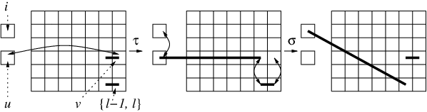
Let be the number of columns of to the left of . Then there are possible choices of . Now where (as is an arbitrary element in its column of ) and permutes the pairs in each of the first double columns of arbitrarily, and in the last double column sends to and to and then permutes the other pairs arbitrarily. Note that . Hence (arguing as in earlier cases) we get a contribution of
Subcase 4(b): Suppose that is a box of which is above some column of but to the left of . Then the only way to use row and column permutations not involving (which we have already used to position ) to connect and (or ) is by some pair and similar to that shown in Figure 14. But (as illustrated) any such pair does not preserve the remaining edges in . Hence this subcase cannot arise.

Subcase 4(c): Finally we are left with the subcase where after action by the element is in a box of which is either in the same column as or in the same column as . In this case where and . Also, where (as is an arbitrary element in its column of ) and either or . If is the number of columns above in then there are choices for the position of . Note that here and so . Hence, in this case we get a contribution of
Note that the final sets of permutations obtained in Subcases 4(a) and 4(c) are disjoint, so there is no double counting in these contributions. Now on adding up all contributions from Cases 1–4 we see that the coefficient of inside of is given by
The content of the top left box of the partition inside the partition is given by . Thus we have proved that this coefficient is a non-zero multiple of as required. ∎
6. The blocks of the Brauer algebra
In section 4 we saw that a necessary condition for two weights and to be in the same block was that the pair was balanced. We will now show that this condition is also sufficient. The key idea will be to construct from any partition in a balanced pair with some a partition and a homomorphism connecting and . This will allow us to proceed by induction.
Given a partition we denote by the set of addable boxes of (i.e. the set of boxes which may be added to such that the new shape is still a partition). Similarly we denote by the set of removable boxes of . If then we denote the set of boxes in which are also boxes of by . Distinct boxes in (respectively in ) have distinct contents, and we will identify such boxes by their contents. We will order the boxes in with a given content by saying that box is smaller than box if appears on an earlier row than .
Definition 6.1.
Suppose that is a balanced pair. For each we wish to consider , the -maximal balanced subpartition between and . This is the maximal partition such that does not contain and and form a balanced pair. We will construct by recursively defining a series of skew partitions which will eventually equal the skew partition . There is by the pairing condition a maximal box (i.e. all others smaller) with content such that . Let . Given , we set
where is the set of boxes in such that is to the right of or below a box in , and is the set of boxes in such that for some and is maximal with such content among the boxes of not already in .
This iterative process eventually stabilises, and we obtain which is a (possibly disconnected) subset of the edge of , having width one. (In particular it does not contain two boxes with the same content.) If is even and does not contain a vertical pair of boxes with content and , or is odd and does not contain a box of content then we set . Otherwise if is even we set
| (16) |
where are the maximal boxes in of content and not in , and if is odd we set
| (17) |
where is the maximal box in of content not in . This new skew partition is not necessarily stable under the addition of boxes and as above, and we repeat that process again until the skew partition eventually stabilises at some step . We then set . Thus is a removable subset of having width at most two (so at most two boxes with any given content).

Example 6.2.
We will now consider several examples of this construction. First let and ; this is a balanced pair for . If is any of the removable boxes in Figure 15(a), then is the shaded region shown. For an example where the resulting skew partition is connected, consider and . This is a balanced pair for . If is any of the removable boxes in then the skew partition is the shaded region shown in Figure 15(b). In this case there is a pair of boxes in the skew partition with contents and (i.e. and ), but we do not get a strip of width because these boxes are not vertically aligned.
For an example of the full iterative process consider and . This is a balanced pair for , and after the first part of the iterative process the skew partition stabilises into the lightly shaded region shown in Figure 16(a). However, we now have a vertical pair in the skew partition with contents and (i.e. and ). Thus we have to apply (16), and add the darkly shaded boxes with content and to this skew partition. The complement of this is no longer a partition, so we remove the remaining darkly shaded region by one further application of the iterative procedure.

Definition 6.3.
We now wish to define a maximal balanced subpartition between and , which we will denote by . Having constructed a skew partition for each removable box of , we partially order this collection by inclusion. We then take to be some minimal element of this set.
Example 6.4.
To see a non-trivial example of this choice, consider and . This is a balanced pair for , but has several different associated skew partitions. If we take to be one of the removable boxes labelled by or then equals the entire shaded region in Figure 16(b). However, if we take to be any of the other removable boxes then consists of the six darkly shaded boxes. As , we take to equal in this case, and hence . (Note that if this example had one additional box of content between the two darkly shaded regions, then we would have to apply (17) and this box would have associated skew partition all of the darkly shaded region together with itself and the diagonally adjacent box with content .)
The importance of this construction is given by
Theorem 6.5.
If is a balanced pair, then for any maximal balanced subpartition between and we have
Proof.
As usual, we may assume that is a partition of . Pick with maximal. (Note that there are at most two such boxes.) If is even and or then is one of the two cases in Figure 17(a) or (b), while if is odd and then is as in Figure 17(c). In each of these cases there is a non-zero homomorphism from to by Theorem 5.2 (or more directly by repeated applications of Frobenius reciprocity). Thus we henceforth assume we are not in any of these cases.

Suppose that is paired with a maximal of content . We will assume that is above, or to the right of, , and leave the (obvious) modifications required for the other case to the reader.
We will be able to proceed by induction using the following claim.
Claim 6.6.
(i) There is no box of content in .
(ii)There is a unique box of content
in .
(iii) If
then the pair and is balanced, and
the associated skew partition is minimal in the set of those of the
form , with in
. Equivalently, for every
in we have
Before proving this claim, we show how it can be used to complete the proof of Theorem 6.5. Note that if has a removable box with content then by minimality , and we are done by Theorem 4.4 and our assumptions on . Thus we assume that there is no such removable box. By Frobenius reciprocity, Corollary 4.8, and Lemma 4.10, we have
By the first two parts of Claim 6.6 this latter Homspace is isomorphic to
and by the final part of Claim 6.6 (and induction) this is non-zero as required.
Thus it only remains to prove Claim 6.6.
Proof of Claim 6.6: (i) First suppose that there is only one box in with content . By construction, if there are any boxes above in then the one with largest content, or its matched pair, is removable. But this contradicts the choice of . The other possibility is that there is a second box in with content , occuping the opposite corner of a two by two square. Arguing as in the previous case, if there are any boxes in above this square then this contradicts the choice of . These two cases are illustrated in Figure 18(a) and (b). In both these cases we deduce that cannot have a removable box of content , as there must be boxes to the right of any such box in .

(ii) Note that if consists of two boxes then the result is obvious, so we assume this is not the case. It is also clear that any addable box of a given content must be unique. Let be the maximal box in with content .
First suppose that has only one box with content , so that we are in the case shown in Figure 18(a). The box paired with in Figure 18(a) must be to the right or above , and hence we are in one of the two configurations shown in Figure 19.

The case in Figure 19(a) is impossible by our assumption on the size of (and minimality), as both and are removable boxes. In the remaining case it is clear that has addable box , as required.
Next suppose that has two boxes with content , so that we are in the case shown in Figure 18(b). As in the previous case, the box paired with must be to the right or above . If it is above then we have a configuration similar to that in Figure 19(a), and hence is a removable box. But this is impossible exactly as for the case in Figure 19(a). Hence must be to the right of , and we must have a configuration as in Figure 20. But this configuration clearly has an addable box, , of content .

(iii) The two partitions and are clearly balanced. For minimality we consider the various cases that can arise. If we are in the case shown in Figure 18(a), then paired boxes are as shown in Figure 19(b). Suppose for a contradiction that is not minimal, and hence contains a smaller skew partition . If does not involve and then it is also contained in , which contradicts the minimality of this original pair. If does involve and then this contradicts being minimal, as contains , which is a smaller sub-skew partition of .
Now consider the case shown in Figure 18(b), where the paired boxes are as in Figure 20. As before, suppose for a contradiction that is not minimal, and hence contains a smaller skew partition . If does not involve and then it is also contained in . If does involve and but not and , then is a removable skew inside . Finally, if involves all of , , , and , then must also involve and . Now the skew obtained from by replacing by can be removed from . In each of these three cases we have found a proper removable skew inside , which contradicts the minimality of . Thus must be minimal, which completes the proof of Claim 6.6, and hence also of Theorem 6.5. ∎
Corollary 6.7.
Two weights and are in the same block of if and only if they are balanced. Each block contains a unique minimal weight.
Proof.
In Corollary 4.8 we proved that two weights in the same block must be balanced. For the reverse implication, we will proceed by induction. By Theorem 6.5, if contains a smaller partition with which it is balanced, then there exists some with a non-zero homomorphism from to . In particular, and will lie in the same block of . Thus it is enough to show that there is a unique minimal partition in the set of partitions which are balanced with .
But if there are two such minimal partitions and , then set . Clearly is a partition, and it forms a balanced pair with both and (and hence with ). This contradicts our assumption of minimality ∎
We conclude this section with a description of the minimal partitions in each block (and hence give a parametrisation of the blocks). We begin by constructing inductively a skew partition related to . Let . Given , consider such that is maximal. Suppose that there does not exist with and . Hence either the set of rows above and including the row containing (if ) or the set of columns to the the left of and including the column containing (if ) cannot be removed. In this case set , respectively . If there exists with and then . This procedure will eventually terminate in the construction of .

Example 6.8.
As an example of this construction, consider and , as illustrated in Figure 21. At the first stage, we take to be the box labelled , and hence remove the first column. Next we take the box labelled , and remove the first two rows. This is followed by the removal of the second column, then the third row, leaving the skew partition illustrated in the figure. As the two remaining removable nodes both have a paired partner (in this case each other) no more rows or columns need be removed, and we have constructed .
Proposition 6.9.
The minimal partitions in each block are precisely those for which either or a single row or column, or is even and consists of two rows, the second of which has final box of content .
Proof.
Clearly if then is minimal in its block. In the remaining cases, removal of any part of can only involve boxes in , and hence to be balanced must involve either a single unpaired box of content or a single vertical pair in the configuration shown in Figure 5(b). But this is impossible. Hence we assume that is not of the form given in the proposition, and will show that is not minimal.
First suppose that is odd. If contains two boxes of content then we can construct a maximal balanced subpartition of , mimicking the process in Definitions 6.1 and 6.3 by starting with . Hence by Theorem 6.5 is non minimal. If only contains one box with content then, again by considering Definitions 6.1 and 6.3 and Theorem 6.5, any removable balanced skew-partition must involve . The assumption also implies that is in the first row or column of .
Suppose that is in the first row of and there is more than one row (the case where is in the first column is similar). If is minimal, then no final segment of this row has a removable paired segment in ; this can only arise if is of the form show in Figure 22 (where shaded areas indicate boxes definitely not in ), where is not paired with any box to the right of . But this means that has content which is impossible, and hence is not minimal.

Now suppose that is even. If contains either of the configurations shown in Figure 23(a) and (b) then we can again construct a maximal balanced subpartition, and by Theorem 6.5 is not minimal.

If contains only one box with content either or then this box is either at the end of the first row or bottom of the first column, which contradicts the definition of . Thus we must have one of the configurations in Figure 23(c) or (d).
In case (c) must lie at the end of the first column, and in case (d) at the end of the first row. Arguing as in the odd case, we see in case (c) that if is minimal then must consist of a single column. However, in case (d), if is minimal then we either have a single row or we are in a similar situation to that in Figure 22 and must have content . But this implies that consists of two rows with the final box having of the second having content , which contradicts our assumptions on .
Thus the only cases where is a minimal partition are those described in the theorem, and so we are done. ∎
Example 6.10.
To illustrate the last result, consider with as shown in Figure 24. The associated is also shown, and has only one row, and it is easy to see that is indeed minimal inside its block.

7. On the submodule structure of certain standard modules
In this section we will show that the structure of standard modules can become arbitrarily complicated (as measured by their Loewy length and number of simples in each Loewy layer). For this it will be sufficient to consider certain special partitions which can be more easily analysed.
Lemma 7.1.
If then
When considering a multi-skew-partition of differences these skew partitions will be listed in the order from top right to bottom left. We will extend the power notation for partitions to multipartitions, so will denote the triple of partitions , , and .
Example 7.2.
To illustrate these definitions we return to the partitions and considered in Figure 7. In this case we have and . Similarly and . The pair is not -balanced for any , and has shape .
We will be interested in -balanced pairs such that the associated skew partition consists entirely of isolated boxes. If are balanced with , denote the matched pairs of boxes in by with respective contents . Let denote the power set of , and for set
For example, .
Theorem 7.3.
Let and be a balanced pair with . Then
and
for all .
Further, denote by the induced lattice in the full submodule lattice of with vertices those simple modules of the form for some . Then is isomorphic to the superset lattice on ; i.e. every submodule of which contains contains for all .
In particular the length of the socle series of is at least and there is a socle series layer containing at least simple modules.
Remark 7.4.
(i) Note that for the induced lattice we are only considering factors of the
form . In general the module will
have many other composition factors. Thus an arrow in
our induced lattice structure is to be understood as representing some
non-trivial extension in with in the head and in
the socle.
(ii) Clearly the final part of
the theorem can be strengthened, but is already enough to show
that standard modules can have arbitrarily large socle series lengths
(and layers of arbitrary width).
Example 7.5.
If and are balanced with then the lattice is illustrated in Figure 25.
Proof.
We proceed by induction on , the result being obvious for . By Frobenius reciprocity we have
| (18) |
By Proposition 2.7 and Corollary 4.8, the only submodule of which can lie in the same block as is isomorphic to , and hence by the inductive hypothesis the right-hand side of (18) is one dimensional. Lemma 4.10 now implies that is a composition factor of . To show that it will be enough to show that there is precisely one copy of this composition factor in (which will necessarily lie in the socle).
By assumption the pair is balanced. We will define the bias of a pair with to be
Thus a balanced pair has zero bias. Consider the restriction . By Proposition 2.7 we have a short exact sequence
| (19) |
Note that has no removable boxes with content for , as this would contradict the existence of an addable node with such a content. Thus the only modules in the sequence (19) with bias are and
By Lemma 7.1 we have that
provided that . But (by the observations on bias above) can only occur in , and by the inductive hypothesis it occurs there precisely once. By varying we deduce that there is at most one copy of each in . But by induction we know that there is a homomorphism from to where , and hence by repeated applications of that there is a homomorphism from to . Hence we see that occurs exactly once in .
Now consider the summand in . This is the only summand of the restriction in which (with ) can arise, and this simple appears in an extension below for all (with ), by the inductive hypothesis. In particular the copy of appearing in appears below in an extension, and this latter simple must come from . It follows that must occur in some extension beneath . This argument works for all and , and hence verifies the claimed submodule structure except for the top two layers. However, these are forced by the structure of standard modules. ∎
8. The case
In this section we will sketch the modifications to the preceding arguments which are required when . The most obvious change is that the idempotents considered thus far no longer exist. This is easily remedied — however a more serious complication is the failure of the algebras to be quasihereditary when is even.

For let be the element illustrated in Figure 26. This is an idempotent for every value of , and satisfies (A1), i.e.
Unfortunately we can no longer prove an analogue of (A2) in general, as the algebras are not quasihereditary. If is odd then there are no problems, and the arguments in the case for (A1-6) go through unchanged. The results in Sections 4-7 also generalise, as the various results needed from [DWH99] include the case , and we thus deduce the block result in this case.
For even, we can no longer appeal directly to the general machinery in [CMPX]. However, the algebras in this case are cellular, and the modules considered by [DWH99] are precisely the cell modules for these algebras. The necessary results coming from the general theory in [CMPX] now have to be verified on an ad hoc basis, but this has been carried out in [DWH99]. Thus, again, the results in Sections 4-7 go through unchanged (noting that it is enough to analyse cell modules when determining blocks by [GL96, (3.9.8)] (see [Mat99, 2.22 Corollary])).
References
- [Bra37] R. Brauer, On algebras which are connected with the semisimple continuous groups, Ann. of Math. 38 (1937), 857–872.
- [Bro55] W. Brown, An algebra related to the orthogonal group, Michigan Math. J. 3 (1955), 1–22.
- [CMPX] A. G. Cox, P. P. Martin, A. E. Parker, and C. Xi, Representation theory of towers of recollement: theory, notes, and examples, J. Algebra, to appear.
- [DDH] R. Dipper, S. Doty, and J. Hu, Brauer’s centralizer algebras, symplectic Schur algebras and Schur-Weyl duality, preprint.
- [Dia] P. Diaconis, Group representations in probability and statistics, Institute of Mathematical Statistics Lecture Notes, Monograph Series 11.
- [Don98] S. Donkin, The -Schur algebra, LMS Lecture Notes Series, vol. 253, Cambridge University Press, 1998.
- [Dot98] S. Doty, Polynomial representations, algebraic monoids, and Schur algebras of classical type, J. Pure Appl. Algebra 123 (1998), 165–199.
- [DWH99] W. F. Doran, D. B. Wales, and P. J. Hanlon, On the semisimplicity of the Brauer centralizer algebras, J. Algebra 211 (1999), 647–685.
- [Ful97] W. Fulton, Young tableaux, LMS Student Texts, vol. 35, Cambridge, 1997.
- [GL96] J. J. Graham and G. I. Lehrer, Cellular algebras, Invent. Math. 123 (1996), 1–34.
- [Gre80] J. A. Green, Polynomial representations of GLn, Lecture Notes in Mathematics 830, Springer, 1980.
- [HP] R. Hartmann and R. Paget, Young modules and filtration multiplicities for Brauer algebras, preprint.
- [HW89a] P. J. Hanlon and D. B. Wales, Eigenvalues connected with Brauer’s centralizer algebras, J. Algebra 121 (1989), 446–476.
- [HW89b] by same author, On the decomposition of Brauer’s centralizer algebras, J. Algebra 121 (1989), 409–445.
- [HW90] by same author, Computing the discriminants of Brauer’s centralizer algebras, Math. Comp. 54 (1990), 771–796.
- [HW94] by same author, A tower construction for the radical in Brauer’s centralizer algebras, J. Algebra 164 (1994), 773–830.
- [JK81] G. D. James and A. Kerber, The representation theory of the Symmetric group, Encyclopedia of Mathematics and its Applications, vol. 16, Addison-Wesley, 1981.
- [Mar91] P. P. Martin, Potts models and related problems in statistical mechanics, World Scientific, Singapore, 1991.
- [Mar96] by same author, The structure of the Partition algebras, J. Algebra 183 (1996), 319–358.
- [Mat99] A. Mathas, Iwahori-Hecke algebras and Schur algebras of the symmetric groups, University lecture series, vol. 15, American Mathematical Society, 1999.
- [MRH04] P. P. Martin and S. Ryom-Hansen, Virtual algebraic Lie theory: Tilting modules and Ringel duals for blob algebras, Proc. LMS 89 (2004), 655–675.
- [MW03] P. P. Martin and D. Woodcock, Generalized blob algebras and alcove geometry, LMS J. of Comp. and Math. 6 (2003), 249–296.
- [Naz96] M. Nazarov, Young’s orthogonal form for Brauer’s centralizer algebra, J. Algebra 182 (1996), 664–693.
- [Oeh01] S. Oehms, Centralizer coalgebras, FRT-construction and symplectic monoids, J. Algebra 244 (2001), 19–44.
- [OR01] R. Orellana and A. Ram, Affine braids, markov traces and the category , preprint, 2001.
- [Rui05] H. Rui, A criterion on the semisimple Brauer algebras, J. Comb. Theory Ser. A 111 (2005), 78–88.
- [Wen88] H. Wenzl, On the structure of Brauer’s centralizer algebra, Ann. Math. 128 (1988), 173–193.
- [Wey46] H. Weyl, The classical groups, their invariants and representations, Priceton University Press, 1946.