Iterative algorithms to approximate canonical Gabor windows: Computational aspects
Abstract
In this paper we investigate the computational aspects of some recently proposed iterative methods for approximating the canonical tight and canonical dual window of a Gabor frame . The iterations start with the window while the iteration steps comprise the window , the iterand , the frame operators and corresponding to and , respectively, and a number of scalars. The structure of the iteration step of the method is determined by the envisaged convergence order of the method. We consider two strategies for scaling the terms in the iteration step: norm scaling, where in each step the windows are normalized, and initial scaling where we only scale in the very beginning. Norm scaling leads to fast, but conditionally convergent methods, while initial scaling leads to unconditionally convergent methods, but with possibly suboptimal convergence constants. The iterations, initially formulated for time-continuous Gabor systems, are considered and tested in a discrete setting in which one passes to the appropriately sampled-and-periodized windows and frame operators. Furthermore, they are compared with respect to accuracy and efficiency with other methods to approximate canonical windows associated with Gabor frames.
Keywords:
Gabor frame, tight window, dual window, iterative method, scaling, adjoint orbit, Zak transform. MSC: 42C15; 41A25; 47A58; 94A121 Introduction
We consider in this paper iterative schemes for the approximation of the canonical tight and canonical dual windows associated with a Gabor frame. We refer to [6, Ch. 8-10] and [11, Ch. 5-9, 11-13] for recent and comprehensive treatments of the theory of Gabor systems and frames; to fix notations and conventions we briefly give here the main features. We denote for and , by the collection of time-frequency shifted windows
| (1.1) |
where for we denote
| (1.2) |
We refer to as the window and to and as the time-shift and frequency-shift parameters, respectively, of the Gabor system . When there are , , called the lower and upper frame bound, respectively, such that for all there holds
| (1.3) |
we call a Gabor frame. When in (1.3) the second inequality holds for all , we have that
| (1.4) |
is well-defined as a bounded, positive, semi-definite linear operator of . We call the frame operator of . The frame operator commutes with all relevant shift operators, i.e., we have for all
| (1.5) |
We shall assume in the remainder of this paper that is a Gabor frame. Thus the frame operator is positive definite and therefore boundedly invertible. There are two windows canonically associated to the Gabor frame . These are the canonical tight window and the canonical dual window , defined by
| , | (1.6) |
respectively. The practical relevance of these windows is that they give rise to Gabor series representations of arbitrary according to
| (1.7) |
where both series are -convergent. Furthermore, the Gabor systems and are Gabor frames themselves with frame operators equal to the identity and , respectively.
The computation of and according to (1.6) requires taking the inverse square root and the inverse of the frame operator , respectively. In the often occurring practical case that is a rational number, the frame operator is highly structured which allows relatively efficient methods for computing , see [27]. The computation of is much more awkward, even in the case that is rational, and often requires advanced techniques from numerical linear algebra, see for instance [13].
In [20] the calculus of Gabor frame operators was combined with a use of the spectral mapping theorem and Kantorovich’s inequality to analyze an iteration scheme for the approximation of that was proposed around 1995 by Feichtinger and Strohmer (independently of one another). In this iteration scheme one sets and for
I.
| (1.8) |
where is the frame operator corresponding to . It was shown in [20] that is indeed a Gabor frame, and that converges (at least) quadratically to . From the numerical results in [20] for the case that is the standard Gaussian window and it appears that the resulting method compares favorably with other iterative techniques for computing inverse square roots, [24, 25, 29].
The investigations in [20] were followed by the introduction in [18, 19] of two families of iterative algorithms for the approximation of and , in which the iteration step involves the initial window and the frame operator as well as the current window and frame operator , but frame operator inversion as in (1.8) do not occur. The following instances of these two families were analyzed in [18, 19]. Again we set , and for
II.
| (1.9) |
III.
| (1.10) |
for the approximation of , and
IV.
| (1.11) |
V.
| (1.12) |
for the approximation of .
The algorithms II-V are, contrary to algorithm I, conditionally convergent in the sense that the frame bound ratio of the initial Gabor frame should exceed a certain lower bound. Accordingly, in algorithm II and III we have that converges to quadratically and cubically when and , respectively. In algorithm IV and V we have that converges to quadratically and cubically when and , respectively. A remarkable phenomenon that emerged from the preliminary experiments done with the algorithms around 2002, was the fact that the lower bounds for the algorithms II, III seem far too pessimistic while those for the algorithms IV and V appear to be realistic.
In the algorithms just presented, all computed windows are normalized. We shall refer to this as norm scaling. Another possibility that we will investigate, is to replace all scalars ’s, ’s, ’s and ’s that occur in (1.9-1.12) by , and then initially scale the windows by replacing
| , | (1.13) |
We shall refer to this scaling strategy as initial scaling. If is (an estimate for) the best upper frame bound then the algorithms will be unconditionally convergent, with guaranteed desired convergence order, but with convergence constants that may not be as good as the ones that can be obtained by using the norm scaling as described by (1.9-1.12).
Matrix versions of algorithms II-III without any scaling have been treated in [5]. In [14, 23] the matrix version of algorithm II is considered using norm scaling and a scaling method that approximates the optimal scaling. The matrix version of algorithm IV is known as a Schulz iteration, see [28]. The fact that , and therefore with continuous and positive on the spectrum of , commutes with all relevant shift operators, allows us to formulate the iteration steps on the level of the windows themselves.
In this paper we investigate the algorithms II-V, using both norm and initial scaling, with more emphasis on computational aspects than in [20, 18, 19]. Here it is necessary to consider sampled-and-periodized Gabor systems in the style of [16]. This allows for a formulation and analysis of the algorithms I-V in an entirely similar way as was done in [20, 18, 19]. Thanks to the fact that the involved (canonical) windows and frame operators behave so conveniently under the operations of sampling and periodization, the observations done on the sampled-and-periodized systems are directly relevant to the time-continuous systems. We must restrict here to rational values of , and this gives the frame operator additional structure which can be exploited in the computations as dictated by the recursion steps, also see [2, 27, 30] for this matter.
The notions "smart" (or, rather, "smart but risky") and "safe" (or, rather, "safe but conservative") were introduced in a casual way in [19] to distinguish between cases where the stationary point(s) of the function transforming (frame) operators according to (4.2), (4.9) has a good chance to be well-placed in the middle of and on the "safe" side of the relevant spectral set, respectively. In the present paper, we choose to refer to the strategies leading to smart and safe modes as "norm scaling" and "initial scaling", respectively, and discard the terms "smart" and "safe" altogether.
2 Paper outline and results
In Section 3 and 4 we present the basic results of [18, 19] on transforming into , where is a function positive and continuous on , so as to obtain a window whose frame operator (for approximating ) or the operator (for approximating ) is closer to (a multiple of) the identity than itself. Here we recall that has frame operator and that has frame operator . Thus we relate the operators and and their frame bounds, and we present a bound for the distance between (the normed) and in terms of the frame bounds of . Similarly, we relate the frame bounds of and the minimum and maximum of , and we present a bound for the difference between (the normed) and in terms of the latter minimum and maximum. Next, in Section 4, the choice of is specified so as to accommodate the recursions of type II, III and of type IV, V which gives us a means to monitor the frame bound ratio (for ) and of the ratio between minimum and maximum of (for ) during the iteration process.
In Section 5 we present the algorithms using only initial scaling.
In Section 6 we elaborate on the observation that all algorithms take place in the closed linear span of the adjoint orbit . Here the dual lattice representation of frame operators is relevant as well as an operator norm to measure the distance of (for ) and of (for ) from (a multiple of) the identity. The consideration of the algorithms in the space reveals a fundamental difference between the algorithms for computing and that manifests itself in the totally different after-convergence behaviour of the two families of algorithms.
In Section 7 we give some considerations in the Zak transform domain, so as to produce examples of Gabor frames for which a specific algorithm diverges.
In Section 8 we discuss the discretization and finitization aspects (through sampling and periodization) that have to be taken into account since the algorithms are to be tested numerically.
In Section 9 we show how the algorithms can be expressed for discrete, finite Gabor systems, and show that the algorithms are scalar iterations of the singular values of certain matrices. We present an efficient implementation of the iterative algorithms, and we list the window functions we have used to test the algorithms.
In Section 10 we present our experimental results, compare them with what the theory predicts and with other methods to compute tight and dual windows. We provide examples that show the quadratic and cubic convergence of the algorithms, and the exponential divergence of the dual iterations after the initial convergence. We give an example that breaks the norm scaling schemes for both the tight and dual iterations, and show how various error norms of the iteration step behave. Comparisons with other methods are made: We show that the tight iterations are competitive with respect to computing time and superior with respect to precision. Finally, we show that the number of iterations needed for full convergence of the algorithms are dependent on the frame bound ratio, but independent of the structural properties of the discretization. For initial scaling, we show that it is easy to choose a scaling parameter that gives almost optimal convergence.
3 Frame operator calculus and basic inequalities
The basic theory to analyze the recursions appears somewhat scattered in [20, 18, 19]; for the reader’s convenience, we give in Section 3 and 4 a concise yet comprehensive summary of the basic results and ideas. We let be a Gabor frame with frame operator and best frame bounds , , where is the spectrum of . In this section we present the basic inequalities expressing the approximation errors in terms of the (frame) bounds on the involved (frame) operators. These inequalities are a consequence of the calculus of Gabor frame operators, the spectral mapping theorem and Kantorovich’s inequality.
Proposition 1
Let be continuous and positive on , and set . The following holds.
- (i)
is a Gabor frame with frame operator and best frame bounds
, (3.1) Furthermore,
(3.2) and
(3.3) - (ii)
Let , and
(3.4) (3.5) Then
, (3.6) and
(3.7)
The basic result (i) gives us a clue how to produce a good approximation of : Take such that is flat on so that the number in (3.3) is close to . Similarly, by the basic result (ii), the number in (3.7) is close to when is such that is flat on , and then we obtain a good approximation of . In the next two subsections, we use this basic result repeatedly with polynomials of fixed degree so as to obtain iterative approximations of and .
4 Norm scaling
4.1 Iterations for approximating
We consider iteration schemes
| (4.1) |
for the approximation of , where is the frame operator of . We use here the basic result (i) repeatedly with
| (4.2) |
For we have that and that
| (4.3) |
where and are the best frame bounds of . The numbers , can be computed and estimated recursively according to , and
| (4.4) | |||||
| (4.5) |
for .
We should choose such that is flat on . To that end there is proposed in [19, Subsec. 5.1] for the choice
| (4.6) |
where the are defined by
| (4.7) |
The motivation for this choice is as follows. The left-hand side of (4.7) is the order Taylor approximation of around , while (when is sufficiently close to 1)
| (4.8) |
Hence should be expected to be flat on , with potentially of order .
When we get the iterations II, III in (1.9), (1.10). It is shown in [18, Sec. 4] and [19, Sec. 6] that for the quantity increases to and that quadratically when , provided that . For it is shown in [18, Sec. 8] that increases to and that cubically when , provided that . In [18, 19] it was observed for that the choice of causes to have one or more stationary points in so that the odds for flatness of on are favourable.
4.2 Iterations for approximating
We consider iteration schemes
| (4.9) |
for the approximation of , where with the frame operator of . It is seen from (4.9) by induction that for some function . Hence by the basic result (i) with , we have that
| , | (4.10) |
and, by the basic result (ii), that
| (4.11) |
where , . A further use of the calculus of frame operators as given by the basic result (i), yields
| (4.12) |
Consequently, the numbers , can be computed and estimated recursively according to , and
| (4.13) | |||||
| (4.14) |
for .
We should choose such that is flat on . To that end there is proposed in [19, Subsec. 5.2] for the choice
| (4.15) |
where the are defined by
| (4.16) |
The motivation for the proposal is similar to the one for the choice of in (4.6) in Subsec. 4.1; we now note that the left-hand side of (4.16) is the order Taylor approximation of around . The implementation of the resulting recurrence step
| (4.17) |
is made feasible by the observation that, thanks to the second item in (3.6), so that
| (4.18) |
When we get the recurrences IV, V in (1.11) and (1.12). It is shown in [18, Sec. 5] and [19, Sec. 7], that for the quantity increases to and that quadratically when , provided that . For it is shown in [18, Sec. 9] that increases to and that cubically when , provided that . In [18, 19] it was observed for that the choice of causes to have one or more stationary points in .
5 Initial scaling
The algorithms II-V are guaranteed to converge when the lower bound ratio of exceeds a certain value. The proofs, as given in [18] and [19], require a careful analysis of the extreme values of the functions on the spectra of the relevant operators and can become quite complicated, especially in the cases of algorithms III, V. However, the algorithms are efficient in the sense that the envisaged convergence order is realized with favourable convergence constants. In practice, as the experiments in Section 10 show, the algorithms II, III turn out to converge in almost all cases, even when the frame bound ratio is close to . However, divergence of the algorithms IV, V occurs much more frequently. In Section 7 we present examples, using the Zak transform, of frames such that algorithm II and IV diverges.
It would be desirable to have versions of the algorithms that are guaranteed to converge, no matter how small the frame bound ratio of the initial frame is (as long as it is positive). In the following, we present the initial scaling versions of the algorithms that converge at the envisaged convergence order , possibly with suboptimal convergence constants. Since we can freely switch scaling strategy, a possible strategy is to initially scale such that convergence is guaranteed, and to continue until one is confident that the relevant condition number exceeds the specific lower bound so that the norm scaling mode can be applied from that point onwards.
The introduction in [19] of the notion of “safe modes” was prompted by an observation by M. Hampejs who prescaled the window (and the frame operator) and deleted all normalization operations in the recursion step of algorithms II, IV. In the present paper, the prescaling is done in such a way that the scaled has its spectrum exclusively in the attraction region of the function describing the simplified recursion. More specifically, we consider the iteration steps as given in Subsections 4.1, 4.2, with all ’s and ’s equal to . The ’s thus obtained are independent of and are given by
and
| (5.4) |
respectively. The relevant spectra transform by the spectral mapping theorem according to
| (5.5) |
and
| (5.6) |
respectively.
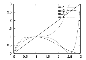
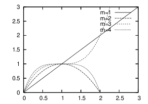
The functions and are order Taylor approximations of and around and , respectively. Hence and approximate around and , respectively. In Fig. 1 we have shown plots of the mappings
| , | (5.7) |
for , respectively. Fig. 1(a) also appears in [5]. In all cases, the point is an attractor for the region . Consequently, when , have spectrum in , the spectra , converge to as , and the convergence is of order in the sense that the ratio of minimum and maximum of the spectra converge to at order . Thus we should replace by and by where is such that to obtain iterations having order convergence to and to , respectively.
To guarantee convergence an estimate of is needed. In [2] a number of upper bounds of are developed for discrete-time, periodic Gabor systems. A convenient upper bound for our purposes follows from the dual lattice representation of the frame operator , see Section 6 for more details, as
| (5.8) |
We make some comments for scaling optimally in the first iteration step. We shall refer to this method as initial optimal scaling. Assume that consists of the entire interval . Consider the tight iterations as described in this Section, and assume that we replace by . Then
| (5.9) | |||||
| (5.10) |
The table shows the optimal scaling constant, or ,
for doing initial scaling of the five iteration types.
| Method. | or |
| I. | |
| II. | |
| III. | |
| IV. | |
| V. |
Initial optimal scaling occurs for that value of for which the ratio is maximal. The optimal value of the scaling parameter for the dual iterations is defined in a similar way. For the five iteration types, the optimal or is shown in Table 2. All these numbers are close to the center of the interval or . It is not hard to show that all optimally scaled operators and have their spectra in the attraction regions given in Figure 1 for the algorithms II-V.
If we scale optimally in each iteration step, and not just the first, we get the best possible convergence constants. However, this method is not practically feasible because of the repeated calculations of frame bounds, and we shall use it only as a reference method. We refer to it as constant optimal scaling, see Fig. 5.
6 Considerations in the adjoint orbit space
We consider the closed linear span of the adjoint orbit . According to the duality principle of Gabor analysis we have that the adjoint orbit is a Riesz basis for (for this matter we refer to [6, Secs. 3.6 and 9.2], and [11, Ch. 7]). Furthermore, when , the orthogonal projection of onto is given by
| (6.1) |
As a consequence of in all our algorithms, we see that . There is also the Wexler-Raz biorthogonality relation,
| (6.2) |
where is Kronecker’s delta. Finally, there is the following fundamental identity of Gabor analysis. Assume that and that the three Gabor systems , , have finite upper frame bounds. Then we have
| (6.3) |
with absolute convergence at either side. We can regard (6.3) as a representation result for the frame-type operator
| (6.4) |
viz. as
| (6.5) |
where is the unitary operator
| (6.6) |
This is the dual lattice representation (also known as the Janssen representation, see [6, Sec. 7.2] and [11, Corr. 9.3.7]) of the frame operator. In order for (6.5) to be well-defined, we assume that satisfies the so-called Condition A’:
- A’:
(6.7)
see [11, Def. 7.2.1]. If then this is the Condition A introduced by Tolimieri and Orr in [32]. We refer to Appendix A where an instance, relevant in the present context, of a pair satisfying condition A’ is given.
6.1 Estimate for upper frame bound
If satisfies Condition A, the frame operator of has the representation
| (6.8) |
with absolute convergence in the operator norm. Therefore, there is the upper bound
| (6.9) |
for the best upper frame bound of .
6.2 Error measure
We measure convergence of to and by inspecting -distances of the normed windows. This quantity is bounded in terms of the numbers and in (3.3) and (3.7) that measure how close the operators and are to being a multiple of the identity operator. In the converse direction, it would be useful to have a measure on the windows that translates directly to the distance of and to (a multiple of) the identity operator. Such a measure can indeed be found. As to we note that when satisfies Condition A then has the representation
| (6.10) |
whence
| (6.11) |
As to we note that and with there holds by frame operator calculus
| (6.12) |
Hence there is the representation
| (6.13) |
Therefore
| (6.14) |
Note that the quantities of the right-hand sides of (6.11) and (6.14) measure to what extent the Wexler-Raz condition (6.2) is violated. In Appendix A it is shown for , and satisfying condition A that the occurring in (6.11) and the , occurring in (6.14) satisfy condition A and A’, respectively. We shall refer to the right hand sides of (6.11) and (6.14) as the dual lattice norm.
6.3 Influence of out-of-space components
We have seen that all iterands of the algorithms are in . We briefly comment on the impact on the algorithms of having non-zero components orthogonal to (one can think here of round-off errors generating these components). To that end we consider the algorithms II and IV (assuming appropriate scaling has been carried out), and we assume that they have converged to the extent that the operators and agree within machine precision with the identity operator.
As for algorithm II we thus have that
| (6.15) |
within machine precision. Hence, possible out-of-space components in are reproduced within machine precision. As a consequence, we should expect that the error stays at its converged level when the iteration is continued beyond the point where machine precision is reached.
Next we consider algorithm IV using initial scaling so that
| (6.16) |
The term has the representation
| (6.17) |
Furthermore,
| (6.18) |
Hence, to machine precision, and, to machine precision,
| (6.19) |
On the other hand the orthogonal component is per (6.16) multiplied by , i.e., to machine precision,
| (6.20) |
As a consequence, the algorithm starts to diverge beyond the point where machine precision is reached.
The observations just made continue to hold for the more general algorithms in Subsections 4.1 and 4.2. Thus no substantial after-convergence error build-up occurs for the algorithms of Subsection 4.1. For the algorithms of Subsection 4.2, with basic recursion step
| (6.21) |
the terms with odd all lie in , and those with even are given within machine precision by . Since , the out-of-space component in gets multiplied by in each iteration step.
7 Zak domain considerations
We consider the case that with integer such that , and we define the Zak transform as (the extension to of) the mapping
| (7.1) |
We refer to [34] and to [17, Sec. 1.5], for more details on the Zak transform and its role in Gabor analysis.
For we set (when )
| (7.2) |
and
| (7.3) |
where the ∗ denotes conjugate transpose. Now is a Gabor frame, with frame bounds , if and only if we have for almost all , with and the largest and smallest positive real number for which the respective inequalities hold. The frame operator of is “represented” by through the formula
| (7.4) |
with matrix multiplication at each point on the right-hand side of (7.4). This formula extends as follows. Assume that is continuous and positive on . Then
| (7.5) |
which is the basic formula for functional calculus in the Zak transform domain.
We consider in this section the critical case (in Sections 9 and 10 more general rational will be dealt with). Then considerable simplifications occur since all the matrices , reduce to scalars. The formula (7.5) then becomes
| (7.6) |
for . In particular we have
| (7.7) | |||||
| (7.8) | |||||
To illustrate the relevance for the algorithms, we consider algorithms II and IV for all scaling strategies. As to initial scaling, we assume that and are scaled such that has best upper frame bound , which means that everywhere. We let
| , | (7.9) |
Then by functional calculus in the Zak transform domain, the algorithms II and IV (initial scaling) assume the form
| ; | (7.10) |
and
| ; | (7.11) |
respectively, where the relations in (7.10) and (7.11) are to be considered at each point . These recursions are then quite easily analyzed by elementary means. For instance, one sees that the assumption is necessary and sufficient for (7.10) to converge to everywhere, while the assumption is necessary and sufficient for (7.11) to converge to everywhere. Unbounded recursions result when we would have allowed to be larger than and , respectively.
Next we consider algorithms II, IV using norm scaling so that (7.10) and (7.11) are to be replaced by
| ; | (7.12) |
and
| ; | (7.13) |
The norms used here are -norms. We consider the case that
| , | (7.14) |
where are two measurable sets such that , . Then is a Gabor frame with best frame bounds , . Furthermore,
| ; | (7.15) |
We have for both algorithms II and IV that
| , | (7.16) |
where , follow recursions that can be made completely explicit (using that, for instance, , where ). Due to the norming operations in the recursion steps, either recursion stays bounded.
We consider the case that . Then an elementary analysis shows the following: There is a such that for recursion (7.12), (7.16) there holds
- •
,
- •
.
8 Sampling and periodization of Gabor frames
The algorithms considered in this paper and in [20, 18, 19] have been formulated for time-continuous Gabor frames while the tests we perform must take place in a finite setting. The transition from continuous to discrete/finite Gabor frames by sampling and periodization has been discussed in [16] and later in [22, 30], see also [7, Subsec. 8.4] and [6, Secs. 10.2 and 10.3]. Let , be positive integers, and assume that is a Gabor frame with frame bounds , . Furthermore, assume that satisfies the aforementioned condition A and the so-called condition R:
- R:
(8.1)
The conditions R and A are not very restrictive; they are, for instance, satisfied by all members of Feichtinger’s algebra , see [7, comment after Thm. 8.4.2]. Then the system
| (8.2) |
is a discrete Gabor frame with frame bounds , , the dual window of the frame satisfies conditions R and A, and the dual window corresponding to the discrete Gabor system in (8.2) is obtained by sampling :
| (8.3) |
The transition from discrete Gabor frames to discrete, periodic Gabor frames is just as convenient. Assume that we have a such that the discrete Gabor system is a discrete Gabor frame with frame bounds . Let for some positive integers , and define
| (8.4) |
Then the system
| (8.5) |
is a discrete, periodic Gabor system with frame bounds , , the dual window of the discrete Gabor system is in , and the dual window corresponding to the discrete periodic Gabor system in (8.5) is obtained by periodizing :
| (8.6) |
An important extension of these results is given in [7, Subsec. 8.4]. Assume that is analytic in an open neighbourhood containing , where , are frame bounds of the Gabor frame with satisfying condition R and A. Then satisfies R and A as well, and
| (8.7) |
where is the frame operator corresponding to the system in (8.2). The approach in [7, Subsec. 8.4] (which uses the Dunford representation of operators as well as theorems of the Wiener -type) can be mimicked so as to generalize the transition result from discrete Gabor systems as above with to discrete, periodic Gabor systems. Thus, with as above and a discrete Gabor system with , frame bounds , and frame operator , we have and
| (8.8) |
where is the frame operator of the system in (8.5). In particular, we see that the sampling-and-periodization approach is valid for the tight window in which case we should consider .
It follows from the above results that the algorithms can be considered for discrete and for discrete, periodic Gabor frames. The findings for these systems are of direct relevance to the algorithms we have considered for the time-continuous case.
9 Implementational aspects
All implementations are done in the finite, discrete setting of Gabor frames. We denote for and by the collection of time-frequency shifted windows
| (9.1) |
where for we denote
| (9.2) |
Note that it must hold that for some Additionally, we define by
| (9.3) |
With these numbers, the density of the Gabor system can be written as where is a irreducible fraction. It holds that .
9.1 Matrix representation and the SVD
Let be the matrix representation of the synthesis operator of a Gabor frame so that
| (9.4) |
for , . Hence has the column vectors . The matrix representation of the frame operator corresponding to is then given as . Since is a frame we have that has full rank .
Assume that is continuous an positive on . From
| (9.5) |
we have that
| (9.6) |
Furthermore, note that for the Frobenius norm we have since all columns of have norm .
The iterations can be written in terms of the synthesis operator matrices as follows. Denote the synthesis operator matrix corresponding to the Gabor frame by . Then we can write the iteration step for algorithm II with norm scaling as
| (9.7) |
We shall consider the thin SVD of the synthesis operator matrices. Thus we let , where is unitary ( has full rank), is a diagonal matrix with positive diagonal elements and has orthonormal columns. With as above, we compute the thin SVD of as
| (9.8) | |||||
Here we have used that , a basic fact in the functional calculus of matrices. The equation (9.8) shows that has the same right and left singular vectors as , and the singular values transform according to . As a consequence we have,
| , | (9.9) |
for the synthesis operators corresponding to and , respectively, for which we should take and in (9.8). We thus see that we have obtained the matrices occurring in the polar decomposition of and the Moore-Penrose pseudo-inverse of .
A further observation is that where , , are the singular values of . Letting be the singular values of and using that
we can write the iteration step in (9.7) on the level of singular values as
| (9.10) |
where and .
9.2 Factorization of finite, discrete Gabor systems
Similar to the Zibulski-Zeevi representation of the Gabor frame operator in the continuous case, see [34, 35, 17], it is possible to compute the actions of the finite, discrete Gabor frame operator (and also the analysis and synthesis operators) very efficiently. Several equivalent methods exists using almost the same number of operations, but differing in the order. In [4] a finite, discrete version of the Zibulski-Zeevi representation is developed. Another method was developed in [26] and [31]. Unfortunately, [31] contains some errors, which have been corrected in [3]. In the following we shall present the Zak-transform method from [4].
For and such that , we define the finite, discrete Zak transform by
| (9.11) |
The finite, discrete Zak transform is quasi-periodic in its first variable and periodic in the second,
| (9.12) |
see [15] for more details. The values of a finite, discrete Zak-transform on the fundamental domain , can be calculated efficiently by FFT’s of length . To obtain values outside the fundamental domain, the quasi-periodicity relation (9.12) can be used.
We define the matrices of size and the matrices by
| , | (9.13) |
where , and
| (9.14) |
With these definitions is holds that the frame operator of is “represented” by through the formula
| (9.15) |
see [4].
With this efficient representation of the frame operator of a finite, discrete Gabor system, we may express the iterations schemes in the finite, discrete Zak domain. We let
| , | (9.16) |
By functional calculus, algorithm II in the finite, discrete Zak transform takes the form
| ; | (9.17) |
The expressions for the other iterations types are similar.
9.3 Other methods
We have considered two other methods of computing the canonical tight window utilizing the factorization (9.13). To calculate the factorization of the canonical tight window ,, we use an eigenvalue decomposition of the factorization of the frame operator of : For each , compute such that where is unitary and is diagonal and set
| (9.18) |
We shall refer to this method as the EIG method. The other method uses (9.9) applied to the matrices of the factorization: For each , compute such that where is unitary, is diagonal and has orthonormal columns. Then it follows from functional calculus in the Zak transform domain (pretty much as in (9.8); also see (7.5)) that
| (9.19) |
We shall refer to this method as the SVD method.
For computing the canonical dual window we have considered simply inverting the matrices of the factorization of the frame operator:
We shall refer to this as the INV method.
9.4 Implementational costs
The computation of needs to be done before the iteration step. It can be computed using flops. This transforms the initial window into the finite, discrete Zak domain. All computations in this domain are then done by multiplication of and matrices. The transform is unitary from with Euclidean norm into , also with Euclidean norm. This gives an easy way to calculate the norms needed for the norm scaling.
We count the number of real floating point operation needed, and assume that everything is done using complex arithmetics. The flop count for a single iteration step in the transform domain for each of the 5 algorithms can be seen in Table 4.
This table shows the flop count of each of the considered methods.
The flop count does not include the cost of the pre- and post-factorization.
The application of an inverse matrix needed for the algorithms I and
INV is done using a Cholesky factorization followed by two substitutions.
An iteration step of V takes more flops to compute than an iteration
step of III, because we need to compute the two terms and
. The flop counts for EIG and SVD methods are only
approximations, because eigenvalues and singular values can be calculated
by many different methods with different flop counts, and because
the process usually involves an iterative step, see [10].
| Method: | Flop count per iteration: |
| I. | . |
| II. | . |
| III. | . |
| IV. | . |
| V. | . |
| Total flop count: | |
| INV. | . |
| EIG. | . |
| SVD. | . |
A quick comparison show that the iterative methods for computing the tight window are comparable in number of flops to the EIG and SVD methods, if the number of necessary iterations is not to big. For the inverse iterations, the situation is different: Computing the inverse of the block matrices by a direct approach requires only slightly more flops than a single iteration step of algorithm IV, so an iterative method will always use more flops than the direct approach. However, there might be situations were it is not desirable to compute the inverse. For instance, if the initial window has small support then the iteration steps can be performed by multiple passes through a filter bank.
9.5 Stopping criterion
Because of the guaranteed quadratic/cubic convergence of the algorithms, it is possible to devise a simple yet powerful stopping criterion: We consider the difference
| (9.20) |
When this difference is close to the machine precision , the algorithm considered has converged. This is a standard stopping criteria, but using it this way means that we have done exactly one iteration step too much. Therefore, we stop when (9.20) is less that and for the algorithms having quadratic and cubic convergence, respectively.
9.6 Window functions
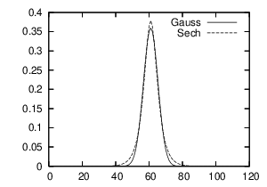
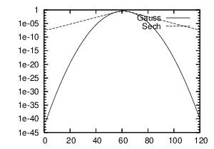
As the basic window functions we shall use the Gaussian and the hyperbolic secant given by
| (9.21) | |||||
| (9.22) |
Both functions are invariant with respect to Fourier transformation. In order to generate a range of functions, we introduce a parameter that dilates the functions by the unitary operator given by
| (9.23) |
Applying this gives
| (9.24) | |||||
| (9.25) |
It holds that the Fourier transform of is and similarly for . As window functions for the testing of the iterative algorithms we shall use finite, discrete versions of these, obtained by the sampling-and-periodization process described in Sec. 8:
| (9.26) | |||||
| (9.27) |
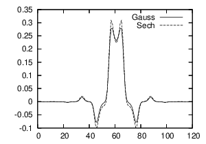
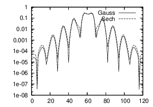
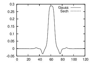
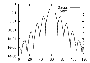
The properties from the continuous setting carry over: The functions have unit norm, and the Discrete Fourier Transform of is and similarly for . For more details on the hyperbolic secant as a Gabor window, see [21]. Figure 2 shows a Gaussian and a hyperbolic secant and their respective canonical dual and tight windows. The different decay properties of the two bell-shaped functions are visible on a logarithmic scale. However, even though the Gaussian and the hyperbolic secant have different decay properties, their canonical windows have almost the same.


To produce examples for which the norm scaling methods diverges, we have constructed a function (MONSTER) which is a Gaussian function modified in such a way that the first singular value, , of the matrix representation of the Gabor synthesis operator that corresponds to a real and symmetric singular vector, is given a large value. The function is shown on Figure 4. This function is a generalization to the case of rational oversampling of the counterexample given in Sec. 7 and exploits that the iterations can be considered as scalar iterations of the singular values of the Gabor synthesis operator, (9.10).
10 Experiments
This section contains the results from the experiments we have done in order to test the algorithms thoroughly and to demonstrate the various aspects of the algorithms that have been shown analytically. The computations have been done in Matlab and Octave, and the full source code is available for download from http://www2.mat.dtu.dk/people/P.Soendergaard/iteralg/. We will show figures demonstrating the important aspects, but since we cannot include all material, the reader is encouraged to download the software and experiment.
10.1 Convergence and divergence of norm scaling

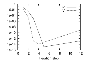
Figure 4 show the convergence behaviour for a well-conditioned problem. The figure shows that algorithm I,II and IV exhibit quadratic convergence, III and V exhibit cubic convergence as proved in Subsections 4.1 and 4.2. Furthermore, the algorithms for computing the tight window stay converged close to the machine precision, while the algorithms for computing the dual window diverge. Algorithm V also diverges faster than IV. This is as proved in Subsection 6.3; the slopes of the two line segments beyond the iteration in Fig. 4(b) corresponds to divergence factors 2 (for IV) and 4 (for V). A visible numerical aspect is that iteration V is not able to reach full precision, because the iterand is quickly affected by the buildup of numerical errors. The convergence behaviour of the algorithms for the initial window being a hyperbolic secant is almost the same.


Two examples of using different scaling strategies is show on Figure 5(a) and 5(b). The figures show that initially scaling by the best scaling constant is as good as using norm scaling and using initial scaling by an easily computable scaling constant results in only 1-2 more iterations than using norm scaling. Comparing these methods to the method using optimal scaling, we see that for a well-conditioned problem then norm-scaling and optimal initial scaling are close to the optimal convergence. For a worse conditioned problem (Fig. 5(b)), optimal scaling clearly outperforms the other methods. However, this observation has little practical relevance, because the computed canonical windows and will have a bad time-frequency localization. Higham [12] uses a scaling strategy for algorithm I that approximates the optimal scaling. This requires an estimate for the smallest eigenvalue of the matrix, but this is easy to obtain since the matrix is inverted as part of the iteration step. For algorithms II-V we cannot use inversions, and so an estimate for the smallest eigenvalue (or lower frame bound) is difficult to obtain. We have therefore not pursued such a method for algorithms II-V.

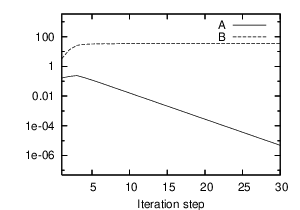
The iterations for computing the tight window are very robust when using norm scaling. It is easy to create examples of Gabor systems with frame bound ratios for which the iterations converge, by using badly dilated Gaussians or by using a constant function with a small amount of noise added. However, by using the function, it is possible to create an example for which the norm scaling iterations diverge. The behaviour of the dual lattice norm and in each iteration step for a run of algorithm II step is shown in Fig. 6(a). It can be seen that the iteration converges to the wrong tight window. Another typical behaviour is that the iteration oscillates between two different functions with the same dual lattice norm. The behaviour of algorithm IV on the same examples is shown in Fig. 6(b), the figure displays the optimal frame bounds of for each iteration step. Here we see exponential convergence of the lower frame bound of to zero.
10.2 Comparison with other methods

Figure 7 show a comparison of the numerical precision of the algorithms for computing the canonical tight window compared to the numerical precision of other standard methods. The stability of the tight iterations proved in Subsection 6.3 is clearly visible. The method based on computing eigenvalues deteriorates quickly as the frame bound ratio increases, while the SVD behaves much better. The eigenvalue method should not be used if the frame bound ratio of the problem is unknown. An explanation for this is that in the SVD method, the singular values are never considered, they are simple set to . Therefore, roundoff errors on the small singular values do not affect the computation, in contrast to the EIG method, where round-off errors on the smallest eigenvalues are magnified because of the inversion of eigenvalues. For more details on the stability of computing eigenvalues and singular values see [1].
The actual running time of the methods is determined by the flop count for each method (see the previous section for details) and of how fast the floating point operations can be executed by a computer. We will not give timings of the iterative algorithms, because we have not created optimal implementations of the algorithms, so timing them makes little sense. We note, however, that the key ingredients in the algorithms are FFTs of small length and matrix multiplications of small size matrices. Fast implementations exists for both algorithms, see [33, 9]. This makes it possible to create efficient implementations of the iterative algorithms.
10.3 Number of iterations
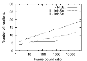
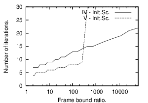
To study how the number of necessary iterations depends on the frame bound ratio of the initial Gabor frame, we have plotted the number of iterations for the algorithms to converge, as a function of the frame bound ratio of the Gabor frame. Figure 8 shows such a plot, using Gaussians to generate Gabor frames with varying frame bound ratios. The jumps in the curves occur when, according to the stopping criteria, an additional iteration step is necessary. Even though algorithm III has cubic convergence, it is almost never able to compete with I. The jump in the graph for V is due to the magnification of round-off errors dominating the convergence, and causing divergence. The same happens for algorithm IV, but for considerable worse frame bound ratios (not visible on the graph). The graphs for the hyperbolic secant look similar.
The number of necessary iterations might also depend on the size of the matrix blocks appearing in the factorization. This issue is slightly problematic to address, since creating a test problem involving bigger matrices also means altering the frame bound ratio. To minimize this effect, we have considered running through the Fibonacci numbers, , such that . This creates a series of irreducible fractions while keeping close to a certain number away from . The result of the test is that the number of necessary iterations seems to be completely independent of the size of the matrix blocks! We have omitted the graphs, as they are simply horizontal lines. For algorithm I, it is proved in [23] that this is indeed the case.
10.4 Choosing an initial scaling

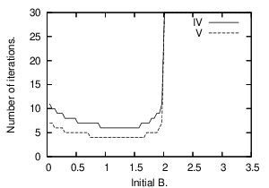
Figure 1 shows that for each iteration type there is a range of values of the upper frame bound of the scaled window, , that will guarantee convergence. Figure 9 shows an example of the effect of prescaling the input window to obtain specific values of . As shown on Fig. 1, algorithm III diverges if is larger than . The dual iterations IV and V diverge if and II has a chaotic behaviour if and diverges if (not shown on the plot).
The choice of that minimizes the number of iterations is to choose according to Table 2. An estimate for this is difficult to calculate, as it involves an estimate for the lower frame bound. Fortunately, as can be seen on Fig. 9 there is a large region around the optimal scaling point, where only 1 or 2 extra iterations are needed.
Appendix A A result on Condition A’
Proposition 2
Assume that is a Gabor frame that satisfies condition A, where . Also assume that is analytic around and positive on , where , are lower, upper frame bounds of . Finally, let where is the frame operator corresponding to . Then satisfies the Condition A’, i.e.,
| (A.1) |
[Proof] We have for that
| (A.2) | |||||
We know that is a Gabor frame. Now take such that and have finite upper frame bounds. Then by the fundamental identity of Gabor analysis, see [17, Subsecs. 1.4.1 and 1.4.2],
| (A.3) |
with absolute convergence on either side of (A.3) . Thus has the dual lattice representation
| (A.4) |
Now let . This is analytic around and positive on . By functional calculus of frame operators in the time-frequency domain, see [7, Sec. 8.3], there holds that has also the dual lattice representation
| (A.5) |
where is the analysis operator with respect to the dual lattice, defined for , by
| (A.6) |
It follows from the proof of [7, Thm. 4.3], in particular from uniform boundedness of (8.4.14) (with instead of ), that
| (A.7) |
By uniqueness of the coefficients in the dual lattice representation (just consider a well-behaved such that is a tight frame, i.e. such that , , is an orthogonal set of functions), it follows that , as required. ††: It is implicit in the statement and proof of [7, Thm 4.3] that the of the above result is such that condition A is satisfied by .
References
- [1] E. Anderson, Z. Bai, C. Bischof, L. S. Blackford, J. Demmel, J. Dongarra, J. D. Croz, A. Greenbaum, S. Hammarling, A. McKenney, and D. Sorensen. LAPACK Users’ Guide, Third Edition. SIAM, Philadelphia, 1999.
- [2] P. Balazs, , H. G. Feichtinger, and G. Kracher. Double preconditioning for Gabor frames. IEEE Trans. Signal Process., submitted for publication, 2005.
- [3] P. Balazs. Regular and Irregular Gabor Multipliers with Application to Psychoacoustic Masking. PhD thesis, Fakultät für Mathematik der Universität Wien, Vienna, june 2005.
- [4] M. J. Bastiaans and M. C. Geilen. On the discrete Gabor transform and the discrete Zak transform. Signal Process., 49(3):151–166, 1996.
- [5] A. Bjorck and C. Bowie. An iterative algorithm for computing the best estimate of an orthogonal matrix. SIAM Jour. Num. Anal., 8(2):358–364, june 1971.
- [6] O. Christensen. An Introduction to Frames and Riesz Bases. Birkhäuser, 2003.
- [7] O. Christensen and T. Strohmer. Methods for the approximation of the inverse (Gabor frame operator. In H. G. Feichtinger and T. Strohmer, editors, Advances in Gabor Analysis, chapter 8, pages 171–196. Birkhäuser, 2003.
- [8] H. G. Feichtinger and T. Strohmer, editors. Gabor Analysis and Algorithms. Birkhäuser, Boston, 1998.
- [9] M. Frigo and S. G. Johnson. The design and implementation of FFTW3. Proceedings of the IEEE, 93(2):216–231, 2005. special issue on "Program Generation, Optimization, and Platfo rm Adaptation".
- [10] G. H. Golub and C. F. van Loan. Matrix computations, third edition. John Hopkins University Press, 1996.
- [11] K. Gröchenig. Foundations of Time-Frequency Analysis. Birkhäuser, 2001.
- [12] N. J. Higham. Computing the polar decomposition—with applications. SIAM J. Sci. Statist. Comput., 7(4):1160–1174, Oct. 1986.
- [13] N. J. Higham. A new sqrtm for MATLAB. Numerical Analysis Report No. 336, Manchester Centre for Computational Mathematics, Manchester, England, Jan. 1999.
- [14] N. J. Higham and R. S. Schreiber. Fast polar decomposition of an arbitrary matrix. SIAM J. Sci. Statist. Comput., 11(4):648–655, July 1990.
- [15] A. J. E. M. Janssen. Duality and biorthogonality for discrete-time Weyl-Heisenberg frames. Unclassified report, Philips Electronics, 002/94.
- [16] A. J. E. M. Janssen. From continuous to discrete Weyl-Heisenberg frames through sampling. J. Fourier Anal. Appl., 3(5):583–596, 1997.
- [17] A. J. E. M. Janssen. The duality condition for Weyl-Heisenberg frames. In Feichtinger and Strohmer [8], chapter 1, pages 33–84.
- [18] A. J. E. M. Janssen. Analysis of some fast algorithms to compute canonical windows for Gabor frames. Unpublished, 2002.
- [19] A. J. E. M. Janssen. Some iterative algorithms to compute canonical windows for Gabor frames. In Proceedings of IMS Workshop on Time-Frequency Analysis and Applications, Singapore, September 2003.
- [20] A. J. E. M. Janssen and T. Strohmer. Characterization and computation of canonical tight windows for Gabor frames. J. Fourier Anal. Appl., 8(1):1–28, 2002.
- [21] A. J. E. M. Janssen and T. Strohmer. Hyperbolic secants yield Gabor frames. Appl. Comput. Harmon. Anal., 12(2):259–267, 2002.
- [22] N. Kaiblinger. Approximation of the Fourier transform and the dual Gabor window. J. Fourier Anal. Appl., 11(1):25–42, 2005.
- [23] C. Kenney and A. J. Laub. On scaling newton’s method for polar decomposition and the matrix sign function. SIAM J. Matrix Anal. Appl., 13(3):688–706, 1992.
- [24] Z. Kovarik. Some iterative methods for improving orthonormality. SIAM J. Num. Anal., 7(3):386–9, 1970.
- [25] S. Lakic. An iterative method for the computation of a matrix inverse square root. ZAMM Z. Angew. Math. Mech., 75(11):867–874, 1995.
- [26] P. Prinz. Calculating the dual Gabor window for general sampling sets. IEEE Trans. Signal Process., 44(8):2078–2082, 1996.
- [27] S. Qiu and H. G. Feichtinger. Discrete gabor structures and optimal representations. IEEE Trans. Signal Process., 43(10):2258 –2268, 1995.
- [28] G. Schulz. Iterative berechnung der reziproken Matrix. ZAMM Z. Angew. Math. Mech., 13:57–59, 1933.
- [29] N. Sherif. On the computation of a matrix inverse square root. Computing (Vienna/New York), 46(4):295–305, 1991.
- [30] P. Søndergaard. Gabor frames by sampling and periodization. Adv. Comput. Math., accepted for publication, 2005.
- [31] T. Strohmer. Numerical algorithms for discrete Gabor expansions. In Feichtinger and Strohmer [8], chapter 8, pages 267–294.
- [32] R. Tolimieri and R. S. Orr. Poisson summation, the ambiguity function, and the theory of Weyl-Heisenberg systems. J. Fourier Anal. Appl., 1(3):233–247, 1995.
- [33] R. C. Whaley, A. Petitet, and J. Dongarra. Automated empirical optimization of software and the ATLAS project. Technical Report UT-CS-00-448, University of Tennessee, Knoxville, TN, Sept. 2000.
- [34] M. Zibulski and Y. Y. Zeevi. Oversampling in the Gabor scheme. IEEE Trans. Signal Process., 41(8):2679–2687, 1993.
- [35] M. Zibulski and Y. Y. Zeevi. Analysis of multiwindow Gabor-type schemes by frame methods. Appl. Comput. Harmon. Anal., 4(2):188–221, 1997.