Bifurcations of stationary measures of random diffeomorphisms

Hicham Zmarrou Ale Jan Homburg Affiliation: KdV Institute for Mathematics Affiliation: University of Amsterdam Affiliation: Plantage Muidergracht 24 Affiliation: 1018 TV Amsterdam Affiliation: The Netherlands

Abstract

Random diffeomorphisms with bounded absolutely continuous noise are known to possess a finite number of stationary measures. We discuss dependence of stationary measures on an auxiliary parameter, thus describing bifurcations of families of random diffeomorphisms. A bifurcation theory is developed under mild regularity assumptions on the diffeomorphisms and the noise distribution (e.g. smooth diffeomorphisms with uniformly distributed additive noise are included). We distinguish bifurcations where the density function of a stationary measure varies discontinuously or where the support of a stationary measure varies discontinuously.

We establish that generic random diffeomorphisms are stable. Densities of stable stationary measures are shown to be smooth and to depend smoothly on an auxiliary parameter, except at bifurcation values. The bifurcation theory explains the occurrence of transients and intermittency as the main bifurcation phenomena in random diffeomorphisms. Quantitative descriptions by means of average escape times from sets as functions of the parameter are provided. Further quantitative properties are described through the speed of decay of correlations as function of the parameter.

Random endomorphisms are studied in one dimension; we show that stable one dimensional random endomorphisms occur open and dense and that in one parameter families bifurcations are typically isolated. We classify codimension one bifurcations for one dimensional random endomorphisms; we distinguish three possible kinds, the random saddle node, the random homoclinic and the random boundary bifurcation. The theory is illustrated on families of random circle diffeomorphisms and random unimodal maps.

^†^† 2000 Mathematics Subject Classification 37A50,37Hxx,37Gxx,60Gxx

1 Introduction

To fix thoughts, consider a single map with an attracting fixed point $P$ . Write $W^{s}(P)$ for its basin of attraction. Adding uniform noise of small amplitude gives a random map with a stationary density with support near $P$ . Increasing the amplitude of the noise leads to a bifurcation when orbits can escape from $W^{s}(P)$ . Two possibilities occur: escaping orbits can or cannot return near $P$ . Escaping orbits lead to transient dynamics if orbits do not return or intermittent dynamics if orbits do return. How can such transitions occur? What are the quantitative characteristics? As a second issue, take a one parameter family of maps that exhibits bifurcations and add small bounded noise to it. What happens to the bifurcation set and in what way do bifurcations in the randomly perturbed map manifest? More generally, one can consider maps and families of maps where noise is an intrinsic part of the description.

It is the purpose of this paper to work out bifurcation theory of random smooth diffeomorphisms from the perspective of stationary measures, providing answers to questions like the ones just stated. The context in which we perform this study is that of points being mapped into bounded domains according to a probability distribution, under some regularity conditions. One can think of points being mapped by a diffeomorphism, defined on some compact manifold $\mathcal{M}$ , followed by a random perturbation. This defines a discrete Markov process on $\mathcal{M}$ given by transition functions $P(x,A)$ providing the chance that a point $x\in\mathcal{M}$ ends up in a Borel set $A\subset\mathcal{M}$ . We will assume that the region where $x$ is mapped into, is a bounded domain $U_{x}$ . We argue that from a modeling point of view there are clear and good reasons to consider bounded noise: in most physical systems random perturbations are limited in their effect.

We indicate the regularity conditions assumed in this paper. A first regularity assumption is smoothness of the density of the transition functions $P(x,A)$ . It is not assumed that this density vanishes on the boundary of its support; densities that are positive on bounded domains to model uniform noise are incorporated. For $y\in\mathcal{M}$ , write $V_{y}$ for the set of points $x\in\mathcal{M}$ that are mapped to domains that include $y$ ;

V_{y}=\{x\in\mathcal{M}\;|\;y\in\text{support }P(x,\cdot)\}.

As a second regularity assumption, we suppose that the sets $V_{y}$ are domains with piecewise smooth boundary varying smooth with $y$ . This assumption is natural in the context of diffeomorphisms followed by noise, but does not hold in the context of endomorphisms (possessing critical points) followed by noise. Precise formulations follow in Section 1.1 below.

An alternative description of the setup is by starting with a collection ${\cal F}$ of maps on $\mathcal{M}$ and a measure on ${\cal F}$ . Maps are drawn randomly, and independently, from ${\cal F}$ according to the given measure. Similarly one can consider maps depending on parameters that are drawn randomly. The random parameters are drawn from a bounded domain according to a given distribution. Typical examples are given by smooth maps $f$ with additive or parametric noise. It will turn out that there is no loss of generality, as far as statistical descriptions are concerned, when considering maps with finitely many random parameters. We address an appendix to the exploration of the range and connections of these definitions.

In the following we will mostly speak of random maps; maps depending on finitely many parameters that are drawn randomly. In the part of the paper developing the general theory, Sections 2 to 7, we assume the maps to be diffeomorphisms. This guarantees the regularity assumptions formulated above in the description as discrete Markov processes to hold. Random endomorphisms are studied in one dimension in Section 8.

Under the mild regularity assumptions, random diffeomorphisms possess finitely many stationary measures, whose support is the closure of an open set and whose density functions (stationary densities) are smooth on all of $\mathcal{M}$ . The stationary densities are flat along the boundary of their support. This has immediate consequences for the statistical properties of orbits: orbits are very rarely found near the boundary of the support of the stationary densities. The main focus of this paper lies then in the description of the dependence of stationary densities on the random diffeomorphisms. This includes describing quantitative characteristics. Motivated by examples discussed below we call a random diffeomorphism stable if its stationary densities and their supports vary continuously with the random diffeomorphism (precise definitions follow shortly). Otherwise we speak of a bifurcation.

Below we introduce the precise setup and present our main results in a series of theorems. The presentation of the material is separated in a section treating random diffeomorphisms (Section 1.1) and a section treating families of random diffeomorphisms (Section 1.2). Various aspects of the bifurcation theory for random diffeomorphisms are presented in Theorems 1.3, 1.6, 1.7, 1.10, 1.13 and 1.16. Appendix A comments on the setup. The main body of the theory is developed in Sections 2 to 7. Sections 2, 3 and 4 contain respectively material on transfer operators, proofs of stability theorems, and discussions of parameter dependence. Sections 5 and 6 develop material on conditionally stationary measures and apply this to compute expected escape times. Section 7 treats the speed of decay of correlations depending on a parameter. Appendix B contains an implicit function theorem used to obtain regularity in the parameter of solutions of integral equations involving the transfer operator.

There is no easy analogous theory for random endomorphisms; stationary measures for random endomorphisms will in general be less regular resulting in different statistical properties. In Section 8 we present a satisfactory theory for one dimensional random endomorphisms, including a classification of possible bifurcations. This extends the general theory in particular by classifying codimension one bifurcations. Typically only finitely many bifurcations occur in one parameter families of random endomorphisms, in contrast to families of deterministic maps. The material on one dimensional random endomorphisms is developed and presented in Section 8.

Section 9 contains two worked out examples of random circle diffeomorphisms and random unimodal maps. In Section 9.1 we consider the standard circle diffeomorphism with small additive noise;

f_{a}(x;\omega)=x+a+\omega+\varepsilon\sin(2\pi x)

(1)

with $x$ on the circle ${\mathbb{R}}/{\mathbb{Z}}$ , for fixed $\varepsilon\in(0,1)$ and a random parameter $\omega$ taken uniformly from a small interval. Section 9.2 discusses as a prototypical example of random endomorphisms on an interval, random logistic maps

f(x;\mu)=(\mu+\omega)x(1-x)

(2)

with multiplicative noise obtained by varying $\omega$ with a uniform distribution in some interval.

There is a large body of literature on stochastic stability (e.g. [53, 37, 7, 2, 3], see also [11]), considering bounded noise as a means to treat properties of single deterministic systems. This is done by letting the noise level decrease to zero. In contrast, we consider maps and families of maps where noise is an intrinsic part of the description.

Previous attempts to study stochastic bifurcations fall into two categories. One way is to consider notions close to the traditional understanding of bifurcations for deterministic dynamics by embedding the random dynamical system into a skew product system. Another way studied frequently in the literature uses singularity theory to describe changes in the density of a stationary measure. This approach has been used to study systems with unbounded noise, often of a Gaussian nature, so that a unique smooth stationary density occurs. See [5] for further discussion. We consider the shape of the stationary densities, but the noise being bounded leaves dynamics part of the picture.

Central in control theory are control sets, that is maximal sets of approximate controllability. The shape of the control sets varies with external parameters, where discontinuous changes are possible. Interpreting the control variable as noise, a relation with the present paper becomes apparent. Discontinuous changes of the control set, interpreted this way, are among the bifurcations identified in this paper. In the context of differential equations depending on a control variable the study of control sets is taken up in [16, 27]. Bifurcation theory for such random differential equations in the spirit of this paper is considered in [34].

1.1 Random diffeomorphisms

The adjective smooth stands for $C^{\infty}$ . Let $\mathcal{M}$ be a smooth $n$ -dimensional compact Riemannian manifold with measure $m$ induced by the Riemannian structure. Let $\Delta$ be a closed domain in $n$ -dimensional Euclidean space. Smoothness of a function $g$ on $\Delta$ is to be understood in the sense that $g$ can be extended to a smooth function on a neighborhood of $\Delta$ .

Definition 1.1

A smooth random map, or random endomorphism, is a smooth map $f:\mathcal{M}\times\Delta\to\mathcal{M}$ , $x\mapsto f(x;\omega)$ , depending on a random parameter $\omega\in\Delta$ drawn from a measure on $\Delta$ with smooth density function $g:\Delta\to{\mathbb{R}}$ , $\omega\mapsto g(\omega)$ . A random diffeomorphism is a smooth random map so that $x\mapsto f(x;\omega)$ is a diffeomorphism for each $\omega$ .

Remark 1.2

Alternatively one can explicitly include the noise distribution $g$ as part of the definition of smooth random map (and speak of a pair $(f,g)$ ). For convenience we consider $g$ given. The results in this paper have direct, easily obtained, analogs if $g$ is allowed to vary.

Note that endomorphisms and diffeomorphisms are always assumed to be smooth. The basic setup we are treating is of points being mapped into bounded domains according to some probability. The following standing assumptions will be made with this setup in mind. The random parameters will be chosen from a region $\Delta$ that is a domain in ${\mathbb{R}}^{n}$ with a piecewise smooth boundary. The number of random parameters is in particular equal to the dimension of the state space $\mathcal{M}$ . The most important examples are where $\Delta$ is the unit ball $\Delta=\{x\in{\mathbb{R}}^{n}\;|\;\|x\|\leq 1\}$ or the unit box $\Delta=\{(x_{1},\ldots,x_{n})\in{\mathbb{R}}^{n}\;|\;|x_{1}|,\ldots,|x_{n}|\leq 1\}$ . Throughout this paper we assume that $\omega\mapsto f(x;\omega)$ is an injective map for each $x$ . Hence $f(x;\Delta)$ is diffeomorphic to $\Delta$ .

Write $\nu$ for the measure on $\Delta$ with density function $g$ . A smooth random map gives rise to a discrete Markov process through the transition functions

P(x,A)=\int_{\{\omega\;|\;f(x;\omega)\in A\}}d\nu(\omega)

(3)

for Borel sets $A$ . With $h_{x}(\omega)=f(x;\omega)$ , the measure $P(x,\cdot)$ equals $(h_{x})_{*}\nu$ defined by $(h_{x})_{*}\nu(A)=\nu(h_{x}^{-1}(A))$ . Vice versa, a discrete Markov process with noise from a ball or a box such that its transition functions have smooth positive densities admits a representation by smooth random maps (depending injectively on a random parameter), see Appendix A. Some cases of parametric noise, where the maps do not depend injectively on the random parameter, do not fall into this setup. We refer to Appendix A for further discussion.

The general theory will be developed for random diffeomorphisms, instead of random endomorphisms. Endomorphisms allow for pathological examples, for instance maps $f(x;\omega)$ that are constant in $x$ . We will however discuss random endomorphisms in one dimension (on a circle or a compact interval) in detail.

With a slight abuse of notation, iterates of $f(x;\omega)$ are given as

f^{k}(x;\omega_{1},\ldots,\omega_{k})=f(f^{k-1}(x;\omega_{1},\ldots,\omega_{k-1});\omega_{k}).

(4)

More generally, write $\Delta^{\mathbb{N}}$ for all infinite sequences ${\boldsymbol{\omega}}=\{\omega_{i}\}_{i\geq 1}$ with each $\omega_{i}\in\Delta$ . Denote $f^{k}(x;{\boldsymbol{\omega}})=f^{k}(x;\omega_{1},\ldots,\omega_{k})$ . Let $\vartheta:\Delta^{\mathbb{N}}\to\Delta^{\mathbb{N}}$ be the left shift operator; $\vartheta\{\omega_{i}\}_{i\geq 1}=\{\omega_{i}\}_{i\geq 2}$ . Consider the skew product system $S:\mathcal{M}\times\Delta^{\mathbb{N}}\to\mathcal{M}\times\Delta^{\mathbb{N}}$ given by

S(x,{\boldsymbol{\omega}})=(f(x;\omega_{1}),\vartheta{\boldsymbol{\omega}}).

(5)

On $\Delta^{\mathbb{N}}$ one considers a measure $\nu^{\infty}$ which is the product of the measure $\nu$ over each $\Delta$ .

With these definitions in mind, we introduce the central notions of stationary measures and ergodic measures. A stationary measure $\mu$ for the smooth random map $f$ is a probability measure on $\mathcal{M}$ with $\mu\times\nu^{\infty}$ S-invariant;

\mu\times\nu^{\infty}(S^{-1}(B))=\mu\times\nu^{\infty}(B)

for Borel sets $B\subset\mathcal{M}\times\Delta^{\mathbb{N}}$ . Equivalently, see [37, 4],

\mu(A)=\int_{\mathcal{M}}P(x,A)d\mu(x)

for Borel sets $A\subset\mathcal{M}$ . We refer to a stationary density as the density of an absolutely continuous stationary measure.

A stationary measure $\mu$ is called ergodic if $\mu\times\nu^{\infty}$ is an ergodic measure for $S$ in the usual sense that invariant subsets of $\mathcal{M}\times\Delta^{\mathbb{N}}$ for $S$ have zero or full measure. See [37] for equivalent formulations. The Birkhoff ergodic theorem tells that for an ergodic stationary measure,

\lim_{n\to\infty}\frac{1}{n}\sum_{i=0}^{n-1}\phi(f^{i}(x;{\boldsymbol{\omega}}))=\int_{\mathcal{M}}\phi(x)d\mu(x)

(6)

for all integrable functions $\phi$ on $\mathcal{M}$ and $\mu\times\nu^{\infty}$ almost every point $(x,{\boldsymbol{\omega}})$ . Taking $\phi=1_{A}$ , the characteristic function of a Borel set $A\subset\mathcal{M}$ , it shows that the relative frequency with which typical orbits visit $A$ is given by $\mu(A)$ .

Write $R^{k}(\mathcal{M})$ for the space of $C^{k}$ random diffeomorphisms $f$ on $\mathcal{M}$ (with $f(x;\omega)$ $C^{k}$ jointly in $x\in\mathcal{M}$ and $\omega\in\Delta$ ), depending on a random parameter from $\Delta$ through a distribution with a $C^{k}$ density function $g$ .

Let a random diffeomorphism $f\in R^{\infty}(\mathcal{M})$ be given. The existence of finitely many ergodic stationary measures for $f$ presented in the following theorem, can be found in [21, Chapter 5] (valid under more general conditions). Similar results are contained in [4]. We add statements on the regularity of the stationary measures valid in our context. Differentiability of stationary densities is also discussed in [49, 8].

Theorem 1.3

The random diffeomorphism $f\in R^{\infty}(\mathcal{M})$ possesses a finite number of ergodic stationary measures $\mu_{1},\ldots,\mu_{m}$ with mutually disjoint supports $E_{i},\ldots,E_{m}$ . All stationary measures are linear combinations of $\mu_{1},\ldots,\mu_{m}$ .

The support $E_{i}$ of $\mu_{i}$ consists of the closure of a finite number of connected open sets $C_{i}^{1},\ldots,C_{i}^{p}$ that are moved cyclically by $f(\cdot;\Delta)$ . The density $\phi_{i}$ of $\mu_{i}$ is a $C^{\infty}$ function on $\mathcal{M}$ .

Proof. See [21, Chapter 5] for the existence proof of cyclically permuted ergodic stationary measures.

Since a point $x$ is mapped to a set $f(x;\Delta)$ diffeomorphic to $\Delta$ , the support $E_{i}$ is the closure of finitely many connected open sets. We claim that the closures of the sets $E_{i}$ , $1\leq i\leq m$ , are mutually disjoint. Suppose on the contrary that $\partial E_{i}$ and $\partial E_{j}$ with $j\neq i$ have a point $z$ in common. Then $z$ is mapped by $f(\cdot;\Delta)$ to the injective image of $\Delta$ . By invariance of $E_{i}$ and $E_{j}$ under $f(\cdot;\Delta)$ , $f(z;\Delta)$ is contained in both $\bar{E_{i}}$ and $\bar{E_{j}}$ , which is not possible.

The regularity statements follow from Proposition 2.3 in Section 2. $\square$

Densities of stationary measures for random endomorphisms are in general not smooth functions, but are less regular (see Section 8). Random endomorphisms without critical points, such as expanding maps, do possess finitely many smooth stationary densities. The proofs for random diffeomorphisms extend to cover such random endomorphisms. The regularity of a stationary density $\phi$ implies that $\phi$ is flat along the boundary of its support $E$ . By the Birkhoff ergodic theorem (applied to the characteristic function of a neighborhood of $\partial E$ ), this means that typical orbits are very infrequently found near the boundary of $E$ .

We introduce a topology on the space $R^{k}(\mathcal{M})$ of random diffeomorphisms in order to be able to compare the dynamics of nearby random diffeomorphisms. Natural topologies on $R^{k}(\mathcal{M})$ are the uniform $C^{k}$ topologies on $C^{k}(\mathcal{M}\times\Delta,\mathcal{M})$ . See e.g. [31] for generalities on these topologies. We will assume $R^{k}(\mathcal{M})$ to be equipped with this topology. Note that the alternative approach through discrete Markov processes suggests a topology using the densities of the transition functions.

Consider $f\in R^{\infty}(\mathcal{M})$ . Write $\mu_{1},\ldots,\mu_{m}$ for the stationary measures of $f\in R^{\infty}(\mathcal{M})$ given by Theorem 1.3.

Definition 1.4

A random endomorphism $f\in R^{\infty}(\mathcal{M})$ is stable if for all $\tilde{f}$ sufficiently close to $f$ , the following two properties are satisfied.

•

For each $i,1\leq i\leq m$ , the random endomorphism $\tilde{f}$ has a stationary measure $\tilde{\mu}_{i}$ whose density is $C^{0}$ close to that of $\mu_{i}$ .
•

The supports of $\tilde{\mu}_{i}$ and $\mu_{i}$ are close in the Hausdorff metric.

We speak of a bifurcation, or a bifurcating random endomorphism, if at least one of these properties is violated.

Definition 1.5

An ergodic stationary measure of $f\in R^{\infty}(\mathcal{M})$ is called isolated or attracting, if there exists an open set $W$ (an isolating neighborhood) containing the support $E$ of $\mu$ , so that $\overline{f(W;\Delta)}\subset W$ and $\mu$ is the only ergodic stationary measure of $f$ with support in $W$ .

For each $\tilde{f}$ close to $f$ is the closure of $\tilde{f}(W;\Delta)$ contained in $W$ . The following stability result shows that nearby random diffeomorphisms have indeed a unique stationary measure with support in $W$ . For bifurcations where stationary measures vary discontinuously the condition of being isolated must therefore be violated. The proof of the following theorem is found in Section 3.

Theorem 1.6

Let $\mu$ be an isolated ergodic stationary measure of $f\in R^{\infty}(\mathcal{M})$ with density $\phi$ with isolating neighborhood $W$ . Then each $\tilde{f}\in R^{\infty}(\mathcal{M})$ sufficiently close to $f$ possesses a unique ergodic stationary measure $\tilde{\mu}$ with support in $W$ . The density $\tilde{\phi}$ of $\tilde{\mu}$ is $C^{\infty}$ close to $\phi$ .

Note though that the above theorem leaves open the possibility that the supports $\tilde{E}$ of $\tilde{\mu}$ and $E$ of $\mu$ are not close in the Hausdorff metric. An illustrative example of this phenomenon is described in Section 9.1.

The following theorem establishes that stable random diffeomorphisms are generic. Its proof is in Section 3. The argument also shows that random diffeomorphisms with a locally constant number of smoothly varying stationary densities (ignoring variations in their support) form an open and dense subset of $R^{\infty}(\mathcal{M})$ .

Theorem 1.7

The set of stable random diffeomorphisms in $R^{\infty}(\mathcal{M})$ contains a countable intersection of open and dense sets.

A thorough description of the dynamics of random circle diffeomorphisms is in Section 9.1. Random diffeomorphisms, and even random endomorphisms, on the circle are shown to form an open and dense set, see Theorem 8.3.

1.2 Families of random diffeomorphisms

Bifurcations are best studied in families depending on finitely many parameters. We will consider families of random diffeomorphisms depending on a single real parameter, where we have the goal to focus on bifurcations that typically occur varying one parameter.

Definition 1.8

A smooth family of random endomorphisms is a family of random endomorphisms $\{f_{a}\}$ depending on parameters $a$ , so that $f_{a}(x;\omega)$ depends smoothly on $(x,\omega,a)$ . A smooth family of random diffeomorphisms is a smooth family of random endomorphisms where each map $f_{a}(\cdot;\omega)$ is a diffeomorphism.

Remark 1.9

Alternatively, one can explicitly include noise densities $g_{a}$ in the definition (considering pairs $(f_{a},g_{a})$ ) with $g_{a}(\omega)$ varying smoothly with $(\omega,a)$ . Compare Remark 1.2. For convenience we consider fixed noise densities, but completely analogous results hold if the noise densities are allowed to vary with $a$ .

Consider a smooth one parameter family $\{f_{a}\}$ of random diffeomorphisms, with $a$ from an interval $I$ . Consider a parameter value $a_{0}$ and an ergodic stationary measure $\mu_{a_{0}}$ with support $E_{a_{0}}$ . The following result extends Theorem 1.6, providing an analogous statement in the context of families. If $\mu_{a_{0}}$ is an isolated ergodic stationary measure then there are ergodic invariant measures $\mu_{a}$ for $a$ near $a_{0}$ with nearby densities.

Theorem 1.10

Suppose $\mu_{a_{0}}$ is an isolated ergodic stationary measure. Then the stationary density $x\mapsto\phi_{a}(x)$ of $\mu_{a}$ depends $C^{\infty}$ on $(x,a)$ .

See Section 4 for the proof. We stress again that the support $E_{a}$ of $\mu_{a}$ can still vary discontinuously in the Hausdorff metric with $a$ . The number of components of the support of the stationary measure can also change, while the stationary density varies smoothly.

Consider a smooth function $\phi$ with support on an isolating neighborhood $W$ for $\mu_{a_{0}}$ and compute averages of $\phi$ along orbits $f^{k}_{a}(x;{\boldsymbol{\omega}})$ . By the Birkhoff ergodic theorem, for typical initial points $x\in W$ and noise sequences ${\boldsymbol{\omega}}$ , the averages lie on a smooth function of $a$ for $a$ near $a_{0}$ .

The two types of bifurcation distinguished in Definition 1.4 gives rise to a particular dynamical phenomenon associated to either intermittency or transients. Consider a family $\{f_{a}\}$ of random diffeomorphisms in $R^{\infty}(\mathcal{M})$ , with $a$ from an open interval $I$ . Suppose that $a_{0}\in I$ is a bifurcation value for $\{f_{a}\}$ involving a stationary measure $\mu$ . Write $\phi$ for the density of $\mu$ . Analogies with deterministic dynamics suggest the following two definitions. In Section 8 we will see that in typical one parameter families of random interval or circle endomorphisms bifurcations are isolated and of these two types.

Definition 1.11

The bifurcation at $a_{0}$ is called an intermittency bifurcation if there is a stationary density $\phi_{a}$ for $\{f_{a}\}$ with $\phi_{a_{0}}=\phi$ and depending continuously on $a$ , so that the support $E_{a}$ of $\phi_{a}$ varies with $a$ , for $a$ near $a_{0}$ , as follows.

•

$E_{a}$ varies continuously for $a$ from one side of $a_{0}$ . Without loss of generality, we assume this to be the case for $a<a_{0}$ .
•

$E_{a}$ is discontinuous at $a=a_{0}$ and $E_{a}$ contains an open set disjoint from $E_{a_{0}}$ for $a>a_{0}$ .

An orbit piece outside a small neighborhood $W$ of $E_{a_{0}}$ is called a burst. Out of the substantial literature on intermittency in dynamics, we point to references [46, 22, 30, 28, 32, 33].

Definition 1.12

The bifurcation at $a_{0}$ is called a transient bifurcation if there is a stationary density $\phi_{a}$ for $\{f_{a}\}$ with $\phi_{a_{0}}=\phi$ for $a$ close to $a_{0}$ from one side of $a_{0}$ (without loss of generality, we assume this to be the case for $a<a_{0}$ ), so that

•

$\phi_{a}$ and its support $E_{a}$ vary continuously with $a$ , for $a\leq a_{0}$ .
•

there is no stationary density near $\phi_{a_{0}}$ for $a$ close to $a_{0}$ and $a>a_{0}$ .

Refer to caption — Figure 1: Typical times series for intermittent dynamics on the left and transient dynamics on the right. The time series are for bifurcation values after the bifurcation took place. The intermittency bifurcation involves interval diffeomorphisms with a single stationary measure; the support consisting of two intervals for a period two cycle bifurcates to form a single interval. In the transient bifurcation one stationary measure out of two stationary measures existing previous to the bifurcation disappears.

We end this section with a quantitative description of time series near intermittent or transient random bifurcations. We do this through the estimation of the expected escape time from a small neighborhood of the support of the bifurcation stationary measure. Estimating the speed of decay of correlations as function of a parameter gives further details of changes through bifurcations.

As before, let $\{f_{a}\}$ be a family of random diffeomorphisms in $R^{\infty}(\mathcal{M})$ , with $a$ from an open interval $I$ . Let $\mu_{a_{0}}$ be a stationary measure of $f_{a_{0}}$ for some $a_{0}\in I$ and let $W$ be an open neighborhood of the support $E_{a_{0}}$ of $\mu_{a_{0}}$ such that no other stationary measure has support intersecting $\overline{W}$ . If $f_{a_{0}}$ is stable, then there is a unique stationary measure $\mu_{a}$ that is the continuation of $\mu_{a_{0}}$ . The stationary measure $\mu_{a}$ has its support in $W$ for $a$ near $a_{0}$ . If $a_{0}$ is a bifurcation value for $\{f_{a}\}$ , iterates $f^{k}_{a}(x;{\boldsymbol{\omega}})$ , for certain $x\in W$ and $a$ near $a_{0}$ , may leave $W$ .

For $x\in W$ and ${\boldsymbol{\omega}}\in\Delta^{\mathbb{N}}$ , define

\chi_{a}(x,{\boldsymbol{\omega}})=\min\{k\;|\;f^{k}_{a}(x;{\boldsymbol{\omega}})\not\in W).

(7)

The following result shows how the average escape time from a neighborhood of the support of a bifurcating stationary measure is more than polynomially large in an unfolding parameter. This makes it difficult to accurately establish the bifurcation parameter value using finite data, even in numerical simulations. It explains the occurrence of very long transients near a transient bifurcation and the very irregular occurrence of bursts in intermittent time series. The proof, in Section 6, relies on the construction of conditionally stationary measures in Section 5.

Theorem 1.13

For each $k>0$ there is a constant $C_{k}>0$ so that

\int_{W}\int_{\Delta^{\mathbb{N}}}\chi_{a}(x,{\boldsymbol{\omega}})d\nu^{\infty}({\boldsymbol{\omega}})dm(x)\geq C_{k}\left|a-a_{0}\right|^{-k}.

A single random map with an isolated measure supported on a single component has exponential decay of correlations as precised in the following proposition. The interest from our perspective in computing the speed of decay of correlations lies in the study of bifurcations where the support of a stationary measure has several components merging. This will be discussed below. Proofs of the following statements are in Section 7. The reader can consult [51, 6] for background on decay of correlations. Write

U^{n}\psi(x)=\int_{\Delta^{n}}\psi\circ f^{n}(x;\omega_{1},\ldots,\omega_{n})d\nu(\omega_{1})\cdots d\nu(\omega_{n}).

Proposition 1.14

Let $f$ be a random map with an isolated stationary measure $\mu$ with connected support. Let $W$ be an isolating neighborhood for $\mu$ . Take $\varphi,\psi\in{\cal L}^{2}(W)$ . Then

\left|\int_{\mathcal{M}}\varphi(x)U^{n}\psi(x)dm(x)-\int_{\mathcal{M}}\varphi(x)dm(x)\int_{\mathcal{M}}\psi(x)d\mu(x)\right|\leq C\eta^{n}

for some $C>0$ , $0<\eta<1$ .

Note that the exponential decay of correlations holds for observables $\varphi,\psi\in{\cal L}^{2}(W)$ , thus including characteristic functions of open sets. On the other hand, our definition involves an average over noise sequences. The following remark addresses this point.

Remark 1.15

For a fixed noise sequence ${\boldsymbol{\omega}}\in\Delta^{\mathbb{N}}$ and nonnegative observables $\varphi,\psi\in{\cal L}^{2}(W)$ , consider

\left|\int_{\mathcal{M}}\varphi(x)\psi\circ f^{n}(x;\omega_{1},\ldots,\omega_{n})(x)dm(x)-\int_{\mathcal{M}}\varphi(x)dm(x)\int_{\mathcal{M}}\psi(x)d\mu(x)\right|.

(8)

By Proposition 1.14, the integral over $\Delta^{n}$ of this expression is bounded by $C\eta^{n}$ . Necessarily, (8) is exponentially small in $n$ for $(\omega_{1},\ldots,\omega_{n})$ outside an exponentially small set. Indeed, choose $\tilde{\eta}$ slightly larger than $\eta$ . Then (8) is larger than $\tilde{\eta}^{n}$ only on a set $S_{n}\subset\Delta^{n}$ with $\nu^{n}(S_{n})<C\eta^{n}/\tilde{\eta}^{n}$ .

We return to a family $\{f_{a}\}$ , $a\in I$ , of random maps. Assume that $f_{a}$ has an isolated measure $\mu_{a}$ for all $a\in I$ with an isolating neighborhood $W$ . Suppose $a_{0}\in I$ is a bifurcation value for an intermittency bifurcation so that

•

the support of $\mu_{a}$ consists of $k$ components for $a\leq a_{0}$ ,
•

the support of $\mu_{a}$ consists of a single component for $a>a_{0}$ .

We incorporate the dependence of $U^{n}$ on $a$ into the notation by writing $U^{n}_{a}$ .

Theorem 1.16

Let $\{f_{a}\}$ be as above. Take $\varphi,\psi\in{\cal L}^{2}(W)$ . There are a constant $C>0$ and a smooth function $a\mapsto\eta_{a}$ with $\eta_{a}=1$ for $a<a_{0}$ and $\eta_{a}<1$ for $a>a_{0}$ , so that

\left|\int_{\mathcal{M}}\varphi(x)U^{n}_{a}\psi(x)dm(x)-\int_{\mathcal{M}}\varphi(x)dm(x)\int_{\mathcal{M}}\psi(x)d\mu_{a}(x)\right|\leq C\eta_{a}^{n}

for $a>a_{0}$ .

The smoothness properties of $\eta_{a}$ imply that $\eta_{a}-1$ is a flat function of $a$ at $a=a_{0}$ . As in the discussion of escape times, that shows how slowly the bifurcation manifests itself in time series when moving the parameter $a$ . Remark 1.15 also applies in the parameter dependent context.

2 Transfer operators

Let $f$ be a random diffeomorphism on the manifold $\mathcal{M}$ . Associated to $f$ is the stochastic transition function,

P(x,A)=\int_{\{\omega\;|\;f(x;\omega)\in A\}}d\nu(\omega)=\int_{\Delta}1_{A}(f(x;\omega))d\nu(\omega),

for Borel sets $A\subset\mathcal{M}$ . Write $h_{x}(\omega)=f(x;\omega)$ , note that $h$ maps $\Delta$ injectively onto $U_{x}=f(x;\Delta)$ . The density

k(x,y)=d\left(h_{x}\right)_{*}\nu/dm

(9)

of $P(x,\cdot)$ vanishes for $y$ outside $U_{x}$ and is a smooth function on its support.

Write ${\cal L}^{1}(\mathcal{M})$ for the space of integrable functions on $\mathcal{M}$ . Define the transfer operator $L$ acting on ${\cal L}^{1}(\mathcal{M})$ by

\int_{A}L\phi(x)dm(x)=\int_{\mathcal{M}}P(x,A)\phi(x)dm(x).

(10)

The transfer operator is a positive linear operator. A stationary density is a fixed point of $L$ .

Define

V_{x}=\{z\in\mathcal{M}\;|\;x\in f(z;\Delta)\},

(11)

which is the set of points in $\mathcal{M}$ that are mapped to $x$ by some random map. The assumptions on the random diffeomorphism $f$ imply that the equation $f(x;\omega)=y$ can be solved for $x$ as a diffeomorphic map of $\omega$ . Therefore $V_{x}$ is diffeomorphic to $\Delta$ and thus a domain with piecewise smooth boundary, depending smoothly on $x$ .

Write $P_{f(\cdot;\omega)}$ for the Perron-Frobenius operator, defined by

\int_{A}P_{f(\cdot;\omega)}\phi(x)dm(x)=\int_{f^{-1}(A;\omega)}\phi(x)dm(x)

(12)

for Borel sets $A$ . That is, for a measure $\mu$ with density $\phi=d\mu/dm$ , $f_{*}\mu$ has density $P_{f}\phi=df_{*}\mu/dm$ (see e.g. [39]). The following lemma gives the transfer operator as an average over the random parameters $\omega$ of the Perron-Frobenius operators for $f(\cdot;\omega)$ and gives an equivalent formulation as an integral over the state space $\mathcal{M}$ .

Lemma 2.1

The transfer operator is given by

L\phi(x)=\int_{\Delta}P_{f(\cdot;\omega)}\phi(x)d\nu(\omega),

(13)

or,

L\phi(x)=\int_{V_{x}}k(y,x)\phi(y)dm(y)

(14)

Proof. By (10), for a continuous function $\psi$ ,

\displaystyle\int_{\mathcal{M}}\psi(x)L\phi(x)dm(x)

\displaystyle=

\displaystyle\int_{\mathcal{M}}\int_{\Delta}\psi(f(x;\omega))\phi(x)d\nu(\omega)dm(x)

Calculate

	$\displaystyle\int_{\mathcal{M}}\int_{\Delta}\psi(f(x;\omega))\phi(x)d\nu(\omega)dm(x)$	$\displaystyle=$	$\displaystyle\int_{\Delta}\int_{\mathcal{M}}\psi(f(x;\omega))\phi(x)dm(x)d\nu(\omega)$
		$\displaystyle=$	$\displaystyle\int_{\Delta}\int_{\mathcal{M}}\psi(x)P_{f(\cdot;\omega)}\phi(x)dm(x)d\nu(\omega)$

This implies (13). Alternatively,

	$\displaystyle\int_{\mathcal{M}}\int_{\Delta}\psi(f(x;\omega))\phi(x)d\nu(\omega)dm(x)$	$\displaystyle=$	$\displaystyle\int_{\mathcal{M}}\int_{U_{x}}\psi(y)\phi(x)k(y,x)dm(y)dm(x)$
		$\displaystyle=$	$\displaystyle\int_{\mathcal{M}}\int_{V_{y}}\psi(y)\phi(x)k(y,x)dm(x)dm(y)$

proves (14). $\square$

Remark 2.2

The transfer operator $L$ preserves integrals, as the following computation shows.

$\displaystyle\int_{\mathcal{M}}L\phi(y)dm(y)$	$\displaystyle=$	$\displaystyle\int_{\mathcal{M}}\int_{V_{y}}k(x,y)\phi(x)dm(x)dm(y)$
	$\displaystyle=$	$\displaystyle\int_{\mathcal{M}}\int_{U_{x}}k(x,y)\phi(x)dm(y)dm(x)$
	$\displaystyle=$	$\displaystyle\int_{\mathcal{M}}\phi(x)dm(x),$

because $\int_{U_{x}}k(x,y)dm(x)=1$ .

Iterating $L$ gives

$\displaystyle L^{2}\phi(x)$	$\displaystyle=$	$\displaystyle\int_{V_{x}}k(z,x)L\phi(z)dz$
	$\displaystyle=$	$\displaystyle\int_{V_{x}}\int_{V_{z}}k(z,x)k(y,z)\phi(y)dydz$
	$\displaystyle=$	$\displaystyle\int_{f^{-1}(V_{x},\Delta)}\int_{V_{x}}k(z,x)k(y,z)dz\phi(y)dy$

which is of a similar form, namely $\int_{f^{-1}(V_{x},\Delta)}k_{2}(y,x)\phi(y)dy$ with $k_{2}(y,x)=\int_{V_{x}}k(z,x)k(y,z)dz$ , as $L\phi(x)$ . Inductively similar expressions are derived for higher iterates of $L$ .

Denote by ${\cal D}(\mathcal{M})=\{\phi\in{\cal L}^{1}(\mathcal{M})\;|\;\phi\geq 0,\int_{\mathcal{M}}\phi(x)dm(x)=1\}$ the space of densities on $\mathcal{M}$ . The above remark shows that $L$ maps ${\cal D}$ into itself. Smoothness of stationary densities is obtained by showing that $L$ maps a space of smooth densities into itself.

Proposition 2.3

The transfer operator $L$ maps $C^{k}(\mathcal{M})$ into itself and is a compact operator on $C^{k}(\mathcal{M})$ .

The number 1 is an eigenvalue of $L$ with equal algebraic and geometric multiplicity $m\geq 1$ . The densities $\phi_{1},\ldots,\phi_{m}$ provide a basis of eigenfunctions with mutually disjoint support. Each eigenfunction $\phi_{i}$ is $C^{\infty}$ and its support consists of a finite number $c_{i}$ of connected components.

Proof. Theorem 1.3 gives the $m$ invariant densities $\phi_{1},\ldots,\phi_{m}$ . The geometric multiplicity of the eigenvalues 1 is equal to $m$ . Since $L$ preserves the ${\cal L}^{1}$ norm, the algebraic and geometric multiplicity of 1 are equal. To see this, suppose on the contrary that there is a nontrivial vector in $\ker(L-I)^{2}\backslash\ker(L-I)$ . Elementary linear algebra gives the existence of a sequence of vectors $\psi_{n}$ inside $\ker(L-I)^{2}$ converging to an eigenvector $\phi$ , such that $\lim_{n\to\infty}L^{n}\psi_{n}=2\phi$ . Indeed, take $\psi\in\ker(L-I)^{2}$ with $L\psi=\phi+\psi$ and let $\psi_{n}=\frac{1}{n}\psi$ . From $L^{n}(\psi)=n\phi+\psi$ it follows that $L^{n}(\phi+\psi_{n})=2\phi+\psi_{n}$ , which converges to $2\phi$ if $n\to\infty$ . This contradicts the preservation of the ${\cal L}^{1}$ norm by $L$ .

There can be no additional eigenvectors of $L$ that do not correspond to linear combinations of densities. Namely, suppose $\phi$ is an eigenvector taking both positive and negative values. Write $\phi=\phi_{+}-\phi_{-}$ for nonnegative functions $\phi_{+}=\max\{\phi,0\}$ , $\phi_{-}=\max\{-\phi,0\}$ . If $\phi$ is not a linear combinations of densities, the supports of $\phi_{+},\phi_{-}$ cannot be invariant. Since $L$ is positive and preserves the ${\cal L}^{1}$ norm, $(L\phi)_{+}<L\phi_{+}$ so that $\phi$ cannot be an eigenvector.

We will show that $L$ maps ${\cal L}^{1}(\mathcal{M})$ into $C^{0}(\mathcal{M})$ and $C^{i}(\mathcal{M})$ into $C^{i+1}(\mathcal{M})$ . From this it follows that $\phi_{i}\in C^{\infty}(\mathcal{M})$ . Take $\psi\in{\cal L}^{1}(\mathcal{M})$ . Use a chart to identify a neighborhood of $x\in\mathcal{M}$ with an open set in ${\mathbb{R}}^{n}$ . With $h$ a small vector in ${\mathbb{R}}^{n}$ , consider

$\displaystyle L\psi(x+h)-L\psi(x)$	$\displaystyle=$	$\displaystyle\int_{V_{x+h}}k(y,x)\psi(y)dm(y)-\int_{V_{x}}k(y,x)\psi(y)dm(y)$	(15)
	$\displaystyle=$	$\displaystyle\int_{V_{x+h}\cap V_{x}}(k(y,x+h)-k(y,x))\psi(y)dm(y)$
		$\displaystyle+\int_{V_{x+h}\backslash(V_{x+h}\cap V_{x})}k(y,x+h)\psi(y)dm(y)$
		$\displaystyle-\int_{V_{x}\backslash(V_{x+h}\cap V_{x})}k(y,x)\psi(y)dm(y).$

The first term on the right hand side is small for $h$ small by continuity of $k$ and integrability of $\psi$ . The other two terms are small for $h$ small by the continuous dependence of $V_{x}$ on $x$ . Continuity of $L\psi$ follows. Suppose next that $\psi\in C^{0}(\mathcal{M})$ and consider $\frac{1}{|h|}\left(L\psi(x+h)-L\psi(x)\right)$ This equals the right hand side of (15) divided by $|h|$ . Note that

\lim_{h\to 0}\frac{1}{|h|}\int_{V_{x+h}\cap V_{x}}(k(y,x+h)-k(y,x))\psi(y)dm(y)=\int_{V_{x}}\frac{\partial}{\partial x}k(y,x)\frac{h}{|h|}\psi(y)dm(y)

is a continuous function of $x$ . To check continuity of the remaining two terms it suffices to do a local calculation by covering the boundary of $V_{x}$ by finitely many balls and using a partition of unity. Without loss of generality we may assume that near a smooth part of the boundary of $V_{x}$ , $V_{x}$ is bounded from below by the graph of a continuously differentiable function $H_{x}:[0,1]^{n-1}\to{\mathbb{R}}$ . We may also assume that $m$ equals Lebesgue measure on ${\mathbb{R}}^{n}$ . Then

	$\displaystyle\lim_{h\to 0}\frac{1}{\|h\|}\int_{V_{x}\backslash(V_{x+h}\cap V_{x})}k(y,x)\psi(y)dy$	$\displaystyle=$	$\displaystyle\lim_{h\to 0}\frac{1}{\|h\|}\int_{[0,1]^{n-1}}\int_{H_{x}(y_{1})}^{H_{x+h}(y_{1})}k(y_{1},y_{2},x)\psi(y)dy_{2}dy_{1}$
		$\displaystyle=$	$\displaystyle\int_{[0,1]^{n-1}}\frac{\partial}{\partial x}H_{x}(y_{1})\frac{h}{\|h\|}k(y_{1},H_{x}(y_{1}),x)\psi(y_{1},H_{x}(y_{1}))dy_{1}$

is a continuous function of $x$ . The contribution near the finitely many points where $V_{x}$ is not smooth vanishes in the limit $h\to 0$ . Summarizing, $D(L\psi)$ has an expression of the form

D(L\psi)(x)=\int_{V_{x}}\frac{\partial}{\partial x}k(y,x)\psi(y)dm(y)+\int_{\partial V_{x}}n(y,x)k(y,x)\psi(y)dS(y)

(16)

where $n(y,x)$ measures the change of $\partial V_{x}$ in the direction of the unit normal vector to $V_{x}$ and $dS$ is the volume on $\partial V_{x}$ . We remark that the formula is a variant of the transport theorem 7.1.12 and the Gauss theorem 7.2.9 in [1]. It follows that $L\psi$ is continuously differentiable if $\psi$ is continuous. Higher order derivatives are computed inductively. This gives that $L\psi\in C^{k+1}(\mathcal{M})$ for $\psi\in C^{k}(\mathcal{M})$ .

We prove compactness on $C^{k}(\mathcal{M})$ by modifying the argument in [41]. Let $B^{k}(\mathcal{M})$ be the unit sphere in $C^{k}(\mathcal{M})$ . Consider first $k=0$ . By the Arzela-Ascoli theorem, compactness of $L$ on $C^{0}(\mathcal{M})$ follows from the following two properties (compare [54]),

•

for all $x\in\mathcal{M}$ , $\{|L\psi(x)|\;|\;\psi\in B^{0}(\mathcal{M})\}$ is bounded,
•

$LF$ is equicontinuous.

For $\psi\in B^{0}(\mathcal{M})$ , $|L\psi(x)|\leq\int_{\mathcal{M}}k(y,x)dm(y)$ . This is a continuous function of $x$ and hence bounded. This proves the first item. The above computations showing that $L\psi$ is continuously differentiable also show that $\|D(L\psi)(x)\|$ is uniformly bounded on $B^{0}(\mathcal{M})$ . This proves that $LF$ is equicontinuous. Compactness in $C^{k}(\mathcal{M})$ follows similarly by noting that

•

for all $x\in\mathcal{M}$ , $i\leq k$ , $\{\|D^{i}(L\psi)(x)\|\;|\;\psi\in B^{k}(\mathcal{M})\}$ is bounded,
•

$\|D^{k+1}(L\psi)(x)\|$ is uniformly bounded on $B^{k}(\mathcal{M})$ .

$\square$

Remark 2.4

The transfer operator $L$ is compact on the space ${\cal L}^{2}(\mathcal{M})$ of quadratic integrable functions on $\mathcal{M}$ [52, Section X.2] and [19]. The proof of Proposition 2.3, demonstrating that the transfer operator increases regularity of functions, implies that the spectrum of $L$ on ${\cal L}^{2}(\mathcal{M})$ equals that of $L$ on $C^{k}(\mathcal{M})$ .

Remark 2.5

The spectral radius of $L$ is 1, the eigenvalue 1 occurs with multiplicity $m$ equal to the number of stationary measures. The peripheral spectrum on the unit circle consists of eigenvalues $e^{2\pi i/p}$ , $0\leq i<p$ , for each $p$ occurring as the number of connected components of a stationary measure. See [26] and [50, Theorem V.4.9] for a proof.

Proposition 2.6

The transfer operator $L$ as a linear map on $C^{k}(\mathcal{M})$ or ${\cal L}^{2}(\mathcal{M})$ depends continuously on $f\in R^{k}(\mathcal{M})$ .

Proof. Consider $\tilde{f}$ near $f$ . Write $\tilde{L}$ and $L$ for the corresponding transfer operators. We need to prove that $\tilde{L}-L$ has small norm. Consider the transfer operators operating on $C^{k}(\mathcal{M})$ (continuity on ${\cal L}^{2}(\mathcal{M})$ is treated analogously). The transfer operator $\tilde{L}$ is given as $\tilde{L}\phi(x)=\int_{\tilde{V}_{x}}\tilde{k}(y,x)\phi(y)dm(y)$ . For $\phi\in B^{k}(\mathcal{M})$ , the unit sphere in $C^{k}(\mathcal{M})$ ,

\tilde{L}\phi(x)-L\phi(x)=\int_{\tilde{V}_{x}}\tilde{k}(y,x)\phi(y)dm(y)-\int_{V_{x}}k(y,x)\phi(y)dm(y)

is small, uniformly in $x$ , since $\tilde{k}(y,x)$ is close to $k(y,x)$ on $\tilde{V}_{x}\cap V_{x}$ and $\tilde{V}_{x}$ is close to $V_{x}$ . The derivative $D(L\phi)$ is given by (16). An analogous formula holds for $D(\tilde{L}\phi)$ . Since the functions and sets involved in the two formulas for $D(\tilde{L}\phi)$ and $D(L\phi)$ are close, $D(\tilde{L}\phi)(x)$ is uniformly close to $D(L\phi)(x)$ . Closeness of higher order derivatives, up to order $k$ , is treated analogously. Continuity on ${\cal L}^{2}(\mathcal{M})$ is proved analogously. $\square$

Remark 2.7

Consider two nearby random diffeomorphisms $f$ and $\tilde{f}$ from $R^{k}(\mathcal{M})$ . Write $L$ and $\tilde{L}$ for the corresponding transfer operators on $C^{k}(\mathcal{M})$ . Let $\lambda_{1},\ldots,\lambda_{l}$ be a finite set of eigenvalues for $L$ and denote by $F$ the sum of the corresponding generalized eigenspaces. Then $\tilde{L}$ possesses a nearby set of eigenvalues $\tilde{\lambda}_{1},\ldots,\tilde{\lambda}_{l}$ . The sum $\tilde{F}$ of the corresponding generalized eigenspaces is a small perturbation of $F$ (in the sense that $F$ and $\tilde{F}$ have nearby bases). See [35, Theorem IV.3.16].

3 Stable random diffeomorphisms

This section contains the proofs of Theorem 1.6 on stability of isolated stationary measures and Theorem 1.7 establishing generic stability of random diffeomorphisms.

For the restriction of random maps to an isolating neighborhood $W$ we consider the transfer operator acting on functions vanishing outside $W$ and at the boundary of $W$ . Write

C^{k}_{0}(W)=\{f\in C^{k}(\mathcal{M})\;|\;\text{the support of }f\text{ is contained in }\bar{W}\}.

Then $L$ acting on $C^{k}_{0}(W)$ is well defined. The results in the previous section hold for $L$ acting on $C^{k}_{0}(W)$ .

Proof of Theorem 1.6. Recall that the closure of $f(W;\Delta)$ is contained in the isolating neighborhood $W$ . This property extends to random diffeomorphisms sufficiently close to $f$ . Restrict the map $x\mapsto f(x;\omega)$ to $W$ and and consider the transfer operator $L$ acting on $C^{k}_{0}(W)$ . Then $L$ has a single eigenvalue 1. Since the spectrum of the transfer operator varies continuously with the random diffeomorphism at $f$ , the transfer operator corresponding to each nearby random diffeomorphism possesses a single eigenvalue 1. The corresponding eigenvector is near $\phi$ . $\square$

Lemma 3.1

Write $L_{f}$ for the transfer operator on $C^{k}(\mathcal{M})$ for $f\in R^{\infty}(\mathcal{M})$ . Densities of stationary measures vary continuously with $f\in R^{\infty}(\mathcal{M})$ at a random diffeomorphism $\bar{f}$ precisely if the multiplicity of the eigenvalue 1 for $L_{f}$ is locally constant in $f$ for $f$ near $\bar{f}$ .

Proof. Consider $\bar{f}\in R^{\infty}(\mathcal{M})$ with an eigenvalue 1 of multiplicity $m$ . Let $\bar{\mu}_{1},\ldots,\bar{\mu}_{m}$ be the ergodic stationary measures with densities $\bar{\phi}_{1},\ldots,\bar{\phi}_{m}$ . Write $F_{\bar{f}}$ be the direct sum of the lines spanned by $\bar{\phi}_{1},\ldots,\bar{\phi}_{m}$ . By Remark 2.7, the transfer operator for any $f\in R^{\infty}(\mathcal{M})$ sufficiently close to $\bar{f}$ possesses a $m$ -dimensional invariant linear space $F_{f}$ that is the continuation of $F_{\bar{f}}$ .

The spectrum of $L_{f}$ restricted to $F_{f}$ is in general close to 1. Suppose now that all eigenvalues equal 1. Then $\phi\in F_{f}$ implies $L_{f}\phi=\phi$ . Write $\phi=\phi^{+}-\phi^{-}$ with $\phi^{+}=\max\{0,\phi\}$ and $\phi^{-}=\max\{0,-\phi\}$ the positive and negative parts of $\phi$ . Because $L_{f}\geq 0$ and $L_{f}$ preserves the ${\cal L}^{1}$ norm, $(L_{f}\phi)^{+}<L_{f}\phi^{+}$ precisely if $\phi^{-}$ and $\phi^{+}$ are not invariant. Thus $\phi^{+}$ and $\phi^{-}$ are necessarily invariant. It follows that invariant densities are obtained by taking positive parts of invariant eigenfunctions. This way $m$ invariant densities for $f$ near those of $\tilde{f}$ can be obtained, proving the lemma. $\square$

Proof of Theorem 1.7. Consider diffeomorphisms on an open neighborhood $U$ of a random diffeomorphism $\bar{f}\in R^{\infty}(\mathcal{M})$ . Write $m$ for the multiplicity of the eigenvalue 1 for the transfer operator corresponding to $\bar{f}$ . There is a neighborhood $D$ of 1 in the complex plane, so that for $U$ small enough, each $f\in U$ has $m$ eigenvalues counting multiplicity in $D$ . Let $F$ denote the $m$ dimensional invariant linear space corresponding to these eigenvalues. Consider the map that assigns to $f\in U$ the union of the support of all functions in $F$ . By the continuous dependence of $F$ on $f$ , this is a lower semicontinuous set valued mapping and therefore continuous on a set $B_{2}\subset U$ of Baire second category [24].

Consider the map that assigns to random diffeomorphisms $f\in R^{\infty}(\mathcal{M})$ the multiplicity $m(f)$ of the eigenvalue 1 for the corresponding transfer map. By the continuous dependence of eigenvalues of the transfer map on $f$ , the map $m$ is upper semicontinuous. Since $m$ takes on finitely many values, it is continuous on an open and dense subset of $R^{\infty}(\mathcal{M})$ . Indeed, consider $A_{n}=\{f\in R^{\infty}(\mathcal{M})\;|\;m(f)<n\}$ . The set of points of continuity of $m$ , in the vicinity of some map in $R^{\infty}(\mathcal{M})$ , equals the intersection of a finite collection of open and dense sets $A_{n}\cup\left(R^{\infty}(\mathcal{M})\backslash\overline{A_{n}}\right)$ , namely with $n$ ranging over a finite set of positive integers.

With reference to Lemma 3.1, the two above items combined prove the theorem. $\square$

4 Auxiliary parameters

Consider a smooth one parameter family of random diffeomorphisms $x\mapsto f_{a}(x;\omega)$ depending on $a$ from an open interval $I$ in ${\mathbb{R}}$ . The transition map $P$ and its density $k$ depend on $a$ , we write $P_{a}$ and $k_{a}$ . The support $U_{x,a}$ of $k_{a}$ is assumed to vary smoothly with $x$ and $a$ . The density $k_{a}(x,y)$ is a smooth function of $(a,x,y)\in\cup_{a,x}\{a\}\times\{x\}\times U_{x,a}$ in the sense that it can be extended to a smooth function on an open neighborhood. Let $L_{a}$ denote the transfer operator for $f_{a}$ , given by

L_{a}\phi(x)=\int_{V_{x,a}}k_{a}(y,x)\phi(y)dm(y).

(17)

The domain of integration $V_{x,a}=\{y\in\mathcal{M}\;|\;y\in f_{a}(x;\Delta)\}$ depends smoothly on $(x,a)$ .

Proposition 4.1

For $r\geq 0$ , the transfer operator $\phi\mapsto L_{a}\phi$ as a map from $C^{k+r}(\mathcal{M})$ into $C^{k}(\mathcal{M})$ is a $C^{r+1}$ map of $a$ and $\phi$ .

Proof. By Proposition 2.6, $L_{a}$ depends continuously on $a$ . For the derivative of $L_{a}\phi$ with respect to $a$ we find an expression similar to (16),

\frac{\partial}{\partial a}L_{a}\phi(x)=\int_{V_{x,a}}\frac{\partial}{\partial a}k_{a}(y,x)\phi(y)dm(y)+\int_{\partial V_{x,a}}s_{a}(y,x)k_{a}(y,x)\phi(y)dS(y)

(18)

for some smooth function $s_{a}$ . It follows that for $\phi\in C^{k}(\mathcal{M})$ , $\frac{\partial}{\partial a}L_{a}\phi\in C^{k}(\mathcal{M})$ . This implies differentiability of $(\phi,a)\mapsto L_{a}\phi$ for $\phi\in C^{k}(\mathcal{M})$ . Higher differentiability is treated similarly. $\square$

The operator $L_{a}:C^{k}(\mathcal{M})\to C^{k}(\mathcal{M})$ does not depend $C^{2}$ on $a$ , since $\frac{\partial^{2}}{\partial a^{2}}L_{a}\phi$ may not exist if $\phi\in C^{0}(\mathcal{M})$ and $\frac{\partial^{2}}{\partial a^{2}}L_{a}\phi$ is a $C^{k-1}$ function if $\phi\in C^{k}(\mathcal{M})$ . What does hold is that $(x,a)\mapsto L_{a}\phi_{a}(x)$ is $C^{k+1}$ if $(x,a)\mapsto\phi_{a}(x)$ is $C^{k}$ .

Proof of Theorem 1.10. Let $W$ be the isolating neighborhood for $\mu_{a_{0}}$ . For $a$ near $a_{0}$ , $f_{a}(W;\Delta)$ is strictly contained in $W$ and $f_{a}$ has a unique stationary measure with support in $W$ . Restrict $f_{a}$ to $W$ for such values of $a_{0}$ .

Consider the transfer operator $L_{a}$ for $f_{a}$ acting on $C^{k}_{0}(W)$ . Write $F$ for the line in $C^{k}_{0}(W)$ spanned by $\phi_{a_{0}}$ . Then $C^{k}_{0}(W)=F\oplus H^{k}_{0}(W)$ with $H^{k}_{0}(W)$ consisting of $C^{k}$ functions with vanishing integral;

H^{k}_{0}(W)=\{\phi\in C^{k}_{0}(W)\;|\;\int_{\mathcal{M}}\phi(x)dm(x)=0\}.

Write $\phi_{a}$ for the eigenvectors of $L_{a}$ continuing $\phi_{a_{0}}$ provided by Proposition 1.6. Decompose $\phi_{a}=\phi_{a_{0}}+\psi_{a}$ with $\psi_{a}\in H^{k}_{0}(W)$ . Then $\psi_{a}$ is a solution of $L_{a}\psi_{a}=\psi_{a}+\phi_{a_{0}}-L_{a}\phi_{a_{0}}$ . Note that $(x,a)\mapsto\phi_{a_{0}}(x)-L_{a}\phi_{a_{0}}(x)$ is $C^{\infty}$ . The spectrum of ${L_{a_{0}}}\raisebox{-1.72218pt}{$\left|\,{}_{H^{k}_{0}(W)}\right.$}$ is away from 1. Proposition B.3 in Appendix B implies the result. $\square$

5 Conditionally stationary measures

To study average escape times from open sets we make use of conditionally stationary measures, which are measures for which on average a fixed percentage of mass escapes under an iterate. We recall the notion of conditionally invariant measure, see [45, 44, 14, 32] for its use in deterministic dynamics. Let a map $f:\mathcal{M}\to\mathcal{M}$ be given and restrict $f$ to a domain $W\subset\mathcal{M}$ . Let $V\subset W$ be the set of points in $W$ that are mapped into $W$ , points in the complement of $V$ in $W$ are mapped outside $W$ . Consider $f:V\to W$ . A conditionally invariant measure for $f$ on $W$ is a measure $\mu$ on $\mathcal{M}$ so that $\mu(A)=\mu(f^{-1}(A))/\mu(f^{-1}(W))$ for Borel sets $A\subset W$ .

Definition 5.1

Let $f\in R^{\infty}(\mathcal{M})$ . Let $W$ be an open domain in $\mathcal{M}$ . A measure $\bar{\mu}$ on $\overline{W}$ is a conditionally stationary measure if

\bar{\mu}(A)=\left.\int_{W}P(x,A)d\bar{\mu}(x)\right/\int_{W}P(x,W)d\bar{\mu}(x)

for Borel sets $A\subset W$ .

See [23, 40] where this notion is called a quasistationary measure. Note that a conditionally stationary measure is a stationary measure if $\int_{W}P(x,W)d\bar{\mu}(x)=1$ , that is, if the support of the conditionally stationary measure lies inside $\overline{W}$ .

Lemma 5.2

A measure $\bar{\mu}$ on $\overline{W}$ is a conditionally stationary measure for $f$ if and only if $\bar{\mu}\times\nu^{\infty}$ is a conditionally invariant measure for $(f,\vartheta)$ on $\overline{W}\times\Delta^{\mathbb{N}}$ .

Proof. Write $D^{1}(x)=\{{\boldsymbol{\omega}}\in\Delta^{\mathbb{N}}\;|\;f(x;{\boldsymbol{\omega}})\in W\}$ . Consider $S:\cup_{x\in W}(\{x\}\times D^{1}(x))\to W\times\Delta^{\mathbb{N}}$ , $S(x,{\boldsymbol{\omega}})=(f(x;{\omega}),\vartheta{\boldsymbol{\omega}})$ . We must show that the following two statements are equivalent.

$(i)$

$\bar{\mu}\times\nu^{\infty}(S^{-1}(A))\left/\bar{\mu}\times\nu^{\infty}(S^{-1}(W\times\Delta^{\mathbb{N}}))\right.=\bar{\mu}\times\nu^{\infty}(A)$ for Borel sets $A\subset W\times\Delta^{\mathbb{N}}$ .
$(ii)$

$\int_{W}\int_{\Delta}1_{U}(f(x;\omega))d\bar{\mu}(x)d\nu(\omega)/\int_{W}\int_{\Delta}1_{W}(f(x;\omega))d\bar{\mu}(x)d\nu(\omega)=\int_{W}1_{U}(x)d\bar{\mu}(x)$ for Borel sets $U\subset W$ .

Take a Borel set $U\times V$ with $U\subset W$ and $V\subset\Delta^{\mathbb{N}}$ and compute

$\displaystyle\bar{\mu}\times\nu^{\infty}(S^{-1}(U\times V))$	$\displaystyle=$	$\displaystyle\bar{\mu}\times\nu^{\infty}\left(\bigcup_{\omega\in\Delta}f^{-1}(U;\omega)\times\{\omega\}\times V\right)$	(19)
	$\displaystyle=$	$\displaystyle\bar{\mu}\times\nu\left(\bigcup_{\omega\in\Delta}f^{-1}(U;\omega)\times\{\omega\}\right)\nu^{\infty}(V)$
	$\displaystyle=$	$\displaystyle\int_{W}\int_{\Delta}1_{U}(f(x;\omega))d\bar{\mu}(x)d\nu(\omega)\nu^{\infty}(V)$

Further

\displaystyle\bar{\mu}\times\nu^{\infty}(U\times V)

\displaystyle=

\displaystyle\int_{W}1_{U}(x)d\bar{\mu}(x)\nu^{\infty}(V)

(20)

Equations (19) and (20) contain the implication $(i)\Rightarrow(ii)$ when applied for $U\times\Delta^{\mathbb{N}}$ for the enumerator and for $W\times\Delta^{\mathbb{N}}$ for the denominator.

To show that $(ii)$ implies $(i)$ , note that (19) and (20) show that $(i)$ holds for Borel sets $A$ of the form $U\times V$ if $(ii)$ is assumed. Therefore it holds for all Borel sets in $W\times\Delta^{\mathbb{N}}$ . $\square$

We continue with the introduction of transfer operators whose fixed points are the densities of conditionally stationary measures. The transfer operator $\bar{L}$ , defined for functions in ${\cal L}^{1}(\overline{W})$ with integral 1, is given by

\bar{L}(\phi)=1_{\overline{W}}L\phi\left/\int_{W}L\phi(x)dm(x).\right.

(21)

Write $\tilde{L}\phi=1_{\overline{W}}L\phi.$

Proposition 5.3

$\tilde{L}$ maps $C^{0}(\overline{W})$ into itself and is a compact operator on it.

Proof. If $k(x,y)$ denotes the density of the stochastic transition function $P(x,\cdot)$ , then

\tilde{L}\phi(x)=\int_{\overline{W}\cap V_{x}}k(y,x)\phi(y)dm(y).

Note that $\overline{W}\cap V_{x}$ depends continuously on $x$ . Recall from the proof of Proposition 2.3 that we must show that

•

for all $x\in\overline{W}$ , $\{|\tilde{L}\psi(x)|\;|\;\psi\in B^{0}(\overline{W})\}$ is bounded,
•

$\tilde{L}F$ is equicontinuous.

Here $B^{0}(\overline{W})$ is the unit sphere in $C^{0}(\overline{W})$ . The first item follows as before: $|\tilde{L}\psi(x)|\leq\int_{W}k(y,x)dm(y)$ is bounded by a continuous function and thus bounded. For the second item we must show that for each $\epsilon>0$ there is $\delta>0$ so that for all $x\in\overline{W}$ , $\psi\in B^{0}(\overline{W})$ , $|\tilde{L}\psi(x+h)-\tilde{L}\psi(x)|<\epsilon$ if $|h|<\delta$ . Recall, see(15),

$\displaystyle\tilde{L}\psi(x+h)-\tilde{L}\psi(x)$	$\displaystyle=$	$\displaystyle\int_{W\cap V_{x+h}\cap V_{x}}(k(y,x+h)-k(y,x))\psi(y)dm(y)$
		$\displaystyle+\int_{W\cap V_{x+h}\backslash(W\cap V_{x+h}\cap V_{x})}k(y,x+h)\psi(y)dm(y)$
		$\displaystyle-\int_{W\cap V_{x}\backslash(W\cap V_{x+h}\cap V_{x})}k(y,x)\psi(y)dm(y).$

Now

|\int_{W\cap V_{x+h}\cap V_{x}}(k(y,x+h)-k(y,x))\psi(y)dm(y)|\leq\int_{W\cap V_{x+h}\cap V_{x}}|k(y,x+h)-k(y,x)|dm(y),

which is small for $|h|$ small by uniform continuity of $k$ . And

|\int_{W\cap V_{x+h}\backslash(W\cap V_{x+h}\cap V_{x})}k(y,x+h)\psi(y)dm(y)|\leq\int_{W\cap V_{x+h}\backslash(W\cap V_{x+h}\cap V_{x})}|k(y,x+h)|dm(y)

is small for $|h|$ small by boundedness of $k$ and uniform continuity of the volume of $V_{x}$ in $x$ . Similarly for the third term. This proves equicontinuity. $\square$

Recall from Proposition 2.6 that $L$ depends continuously on the random diffeomorphism. The same argument shows that $\tilde{L}$ depends continuously on the random diffeomorphism.

Proposition 5.4

The transfer operator $\tilde{L}$ as a linear map on $C^{0}(\mathcal{M})$ depends continuously on $f\in R^{k}(\mathcal{M})$ .

We obtain conditionally stationary measures by a perturbation argument, perturbing from an invariant measure. We do not develop general existence results for conditionally stationary measures, as such general results are not needed for our purposes. Let $\{f_{a}\}$ be a family of random diffeomorphisms depending on a real parameter $a\in I$ . Consider, for $a_{0}\in I$ , a stationary density $\phi_{a_{0}}$ with support $E_{a_{0}}$ . Let $W$ be a neighborhood of $E_{a_{0}}$ disjoint from the supports of possible other stationary densities of $f_{a_{0}}$ .

Proposition 5.5

For $a$ close to $a_{0}$ , $f_{a}$ possesses a conditionally stationary density $\bar{\phi}_{a}$ on $W$ , with $\bar{\phi}_{a_{0}}=\phi_{a_{0}}$ and $(x,a)\mapsto\bar{\phi}_{a}(x)$ continuous in $(x,a)$ . One has

\tilde{L}\bar{\phi}_{a}=\alpha(a)\bar{\phi}_{a},

where $\alpha(a)=\int_{W}L_{a}\bar{\phi}_{a}(x)dm(x)$ depends continuously on $a$ .

Proof. The operator $\tilde{L}_{a}$ varies continuously with $a$ and therefore possesses a single eigenvalue close to 1 for $a$ close to $a_{0}$ . The function $\bar{\phi}_{a}$ is the corresponding eigenfunction. $\square$

Recall the definition of the escape time $\chi_{a}(x,{\boldsymbol{\omega}})$ for $x\in W$ and ${\boldsymbol{\omega}}\in\Delta^{\mathbb{N}}$ :

\chi_{a}(x,{\boldsymbol{\omega}})=\min\{k\;|\;f^{k}_{a}(x;{\boldsymbol{\omega}})\not\in W\}.

Lemma 5.6

\int_{W}\int_{\Delta^{\mathbb{N}}}\chi_{a}(x;{\boldsymbol{\omega}})d\nu^{\infty}(\omega)\bar{\phi}_{a}(x)dm(x)=\frac{1}{1-\alpha(a)}.

Proof. Let $S_{a}(x,{\boldsymbol{\omega}})=(f_{a}(x;{\omega}),\vartheta{\boldsymbol{\omega}})$ . Write

D^{n}_{a}=\{(x,{\boldsymbol{\omega}})\;|\;f^{n}_{a}(x;\omega_{1},\ldots,\omega_{n})\in W\}

for the set of points in $W\times\Delta^{\mathbb{N}}$ that remain in $W\times\Delta^{\mathbb{N}}$ for $n$ iterates of $S_{a}$ . The exit set $E^{n}_{a}$ of points that leave $W\times\Delta^{\mathbb{N}}$ in $n$ iterates equals $D^{n-1}_{a}\backslash D^{n}_{a}$ . Thus $\chi_{a}(x,{\boldsymbol{\omega}})=n$ on $E^{n}_{a}$ . Write $\bar{\mu}_{a}$ for the conditionally stationary measure with density $\bar{\phi}_{a}$ . From (19) with $A=W\times\Delta^{\mathbb{N}}$ we get

$\displaystyle\alpha(a)$	$\displaystyle=$	$\displaystyle\int_{W}P(x,W)d\bar{\mu}_{a}(x)$
	$\displaystyle=$	$\displaystyle\int_{W}\int_{\Delta}1_{W}(f(x;\omega))d\nu(\omega)d\bar{\mu}_{a}(x)$
	$\displaystyle=$	$\displaystyle\bar{\mu}_{a}\times\nu^{\infty}(S_{a}^{-1}(W\times\Delta^{\mathbb{N}})).$

It follows that $\bar{\mu}_{a}\times\nu^{\infty}(E^{k}_{a})=\alpha^{k-1}-\alpha^{k}=\alpha^{k-1}(1-\alpha).$ Calculate

$\displaystyle\int_{W}\int_{\Delta^{\mathbb{N}}}\chi_{a}(x;{\boldsymbol{\omega}})d\nu^{\infty}(\omega)d\bar{\mu}_{a}(x)$	$\displaystyle=$	$\displaystyle\sum_{k=1}^{\infty}\bar{\mu}_{a}\times\nu^{\infty}(E^{n}_{a})$
	$\displaystyle=$	$\displaystyle\sum_{k=1}^{\infty}k\alpha^{k-1}(1-\alpha)$
	$\displaystyle=$	$\displaystyle\frac{1}{1-\alpha}.$

$\square$

As a corollary we obtain that the average escape time from $W$ goes to infinity as $a\to a_{0}$ . More precise estimates are derived in the following section.

Proposition 5.7

$\int_{W}\int_{\Delta^{\mathbb{N}}}\chi_{a}(x,{\boldsymbol{\omega}})d\nu^{\infty}({\boldsymbol{\omega}})dm(x)$ converges to $\infty$ as $a\to a_{0}$ .

Proof. Let $E_{a}$ be the interior of the support of $\bar{\phi}_{a}$ .

$\displaystyle\int_{W}\int_{\Delta^{\mathbb{N}}}\chi_{a}(x,{\boldsymbol{\omega}})d\nu^{\infty}({\boldsymbol{\omega}})dm(x)$	$\displaystyle\geq$	$\displaystyle\int_{E_{a}}\int_{\Delta^{\mathbb{N}}}\frac{\chi_{a}(x,{\boldsymbol{\omega}})}{\bar{\phi}_{a}(x)}d\nu^{\infty}({\boldsymbol{\omega}})\bar{\phi}_{a}(x)dm(x)$
	$\displaystyle\geq$	$\displaystyle C\int_{E_{a}}\int_{\Delta^{\mathbb{N}}}\chi_{a}(x,{\boldsymbol{\omega}})d\nu^{\infty}({\boldsymbol{\omega}})\bar{\phi}_{a}(x)dm(x)$
	$\displaystyle=$	$\displaystyle\frac{C}{1-\alpha(a)},$

for $C=1/\max\{x\in W\;|\;\bar{\phi}_{a}(x)\}$ . For $x$ from the support $E_{a_{0}}$ , the image $f_{a_{0}}(x;\Delta)$ is contained in $E_{a_{0}}$ by invariance of $E_{a_{0}}$ . By continuity of $f_{a}$ , $f_{a}(x;\Delta)\subset W$ for $a$ close enough to $a_{0}$ . Since $\bar{\phi}_{a}$ depends continuously on $a$ , $1-\alpha(a)\leq\int_{W\backslash E_{a_{0}}}\bar{\phi}_{a}(x)dm(x)$ converges to $0$ as $a\to a_{0}$ . The proposition follows. $\square$

6 Escape times

In this section estimates for the average escape time from small neighborhoods of the support of a stationary measure that undergoes a bifurcation are derived, as function of the unfolding parameter.

Let $\{(f_{a},g_{a})\}$ , $a\in I$ , be a smooth one parameter family of random diffeomorphisms on $\mathcal{M}$ . Suppose that $a_{0}\in I$ is a bifurcation value for $\{(f_{a},g_{a})\}$ . Let $\mu$ be a stationary measure for $f_{a_{0}}$ involoved in a bifurcation. Let $W$ be a small neighborhood of $E$ . By Proposition 5.5, for $W$ sufficiently close to $E$ and $a$ near $a_{0}$ , $\{(f_{a},g_{a})\}$ possesses a unique conditionally stationary measure $\bar{\mu}_{a}$ with support in $W$ . Write $\bar{\phi}_{a}$ for the density of $\bar{\mu}_{a}$ . The transfer operator $\bar{L}_{a}$ acting on $C^{0}(\overline{W})$ , has $\bar{\phi}_{a}$ as a unique fixed point.

Let $X^{0}$ be the set of points in $\overline{W}$ with $\partial V_{x,a}\cap\partial W\neq\emptyset$ for $x\in X^{0}$ . For $i\geq 0$ , define $X^{i+1}=f(X^{i};\partial\Delta)$ . We suppress the dependence of $X^{i}$ on $a$ from the notation.

Lemma 6.1

If $x_{i}\in X^{i}$ , then for $x_{i+1}\in f(x_{i};\partial\Delta)$ one has $x_{i}\in\partial V_{x_{i+1},a}$ .

Proof. This is clear from the definition. $\square$

At $x\in X^{0}$ , the boundary of $V_{x,a}\cap W$ varies continuously but not smoothly with $(x,a)$ . It follows that $\bar{L}_{a}(\phi)$ cannot be expected to be more than continuous on $X^{0}$ even for smooth $\phi$ .

Lemma 6.2

Suppose that $(x,a)\mapsto\phi_{a}(x)$ is $C^{k}$ outside $X^{0}\cup\cdots\cup X^{k-1}$ , such that derivatives up to order $k$ are bounded and their restrictions to a component of $W\backslash(X^{0}\cup\cdots\cup X^{k-1})$ extend continuously to the boundary of the component. Then $(x,a)\mapsto\bar{L}_{a}\phi_{a}(x)$ is $C^{k+1}$ outside $X^{0}\cup\cdots\cup X^{k}$ . Likewise, derivatives up to order $k+1$ are bounded and their restrictions to a component of $W\backslash(X^{0}\cup\cdots\cup X^{k})$ extend continuously to the boundary of the component.

Proof. For $x\not\in X^{0}$ , the derivative of $\tilde{L}_{a}\phi$ is of the form

D(\tilde{L}_{a}\phi)(x)=\int_{V_{x,a}\cap W}\frac{\partial}{\partial x}k_{a}(y,x)\phi(y)dm(y)+\int_{\partial(V_{x,a}\cap W)}n_{a}(y,x)k_{a}(y,x)\phi(y)dS(y).

(22)

for a smooth function $k_{a}$ and a piecewise smooth function $n_{a}$ (smooth outside the intersection of $\partial W$ with $\partial V_{x,a}$ ). This identity shows that $\tilde{L}_{a}\phi$ is $C^{1}$ with bounded derivatives outside $X^{0}$ , for any $\phi\in C^{0}(\overline{W})$ . The same holds for $\bar{L}_{a}(\phi)$ . Higher order derivatives are treated inductively. Similar to (22) one has

\frac{\partial}{\partial a}\tilde{L}_{a}\phi(x)=\int_{V_{x,a}\cap W}\frac{\partial}{\partial a}k_{a}(y,x)\phi(y)dm(y)+\int_{\partial(V_{x,a}\cap W)}s_{a}(y,x)k_{a}(y,x)\phi(y)dS(y)

(23)

for some piecewise smooth function $s_{a}$ . This shows that $(x,a)\mapsto\tilde{L}_{a}\phi_{a}(x)$ is $C^{1}$ outside $X^{0}$ for continuous functions $(x,a)\mapsto\phi_{a}(x)$ . The derivatives of $(x,a)\mapsto\tilde{L}_{a}\phi_{a}(x)$ on $W\backslash X^{0}$ are bounded; moreover the derivatives on a component of $W\backslash X^{0}$ extend continuously to the boundary of the component.

Higher order derivatives are treated inductively. Suppose that $(x,a)\mapsto\phi_{a}(x)$ is $C^{k}$ outside $X^{0}\cup\cdots\cup X^{k-1}$ , such that derivatives up to order $k$ are bounded and their restrictions to a component of $W\backslash(X^{0}\cup\cdots\cup X^{k-1})$ extend continuously to the boundary of the component. Then $(x,a)\mapsto\tilde{L}_{a}\phi_{a}(x)$ is $C^{k+1}$ outside $X^{0}\cup\cdots\cup X^{k}$ . Likewise, derivatives up to order $k+1$ are bounded and their restrictions to a component of $W\backslash(X^{0}\cup\cdots\cup X^{k})$ extend continuously to the boundary of the component.

The transfer operator $\bar{L}_{a}$ is the composition of the linear map $\tilde{L}_{a}$ and the projection

\Pi(\phi)=\phi/\int_{W}\phi(x)dm(x).

The projection $\Pi$ is a smooth map which is well defined near $\phi_{a_{0}}$ in $C^{0}(\overline{W})$ , a direct computation shows

D\Pi(\phi)h=\frac{1}{\int_{W}\phi(x)dm(x)}h-\frac{\phi}{(\int_{W}\phi(x)dm(x))^{2}}\int_{W}h(x)dm(x).

Also,

\frac{\partial^{i}}{\partial a^{i}}\int_{W}\phi_{a}(x)dm(x)=\int_{W}\frac{\partial^{i}}{\partial a^{i}}\phi_{a}(x)dm(x).

This implies that also $(x,a)\mapsto\bar{L}_{a}(\phi_{a})(x)$ is $C^{k+1}$ outside $X^{0}\cup\cdots\cup X^{k}$ and has bounded derivatives. $\square$

Proposition 6.3

For each $k\geq 1$ , $\bar{\phi}_{a}$ is $C^{k}$ outside $X^{0}\cup\cdots\cup X^{k-1}$ jointly in $(x,a)$ , the derivatives up to order $k$ are uniformly bounded.

Proof. Proposition 5.5 gives that $\bar{\phi}_{a}(x)$ is continuous in $(x,a)$ . Recall that the support $E$ of $\mu$ consists of finitely many, say $k$ , connected components, permuted cyclically by the random diffeomorphism. An iterate of $f_{a_{0}}$ thus maps each component into itself. The restriction of the transfer operator $L^{k}_{a_{0}}$ to a small neighborhood of $E$ has a single eigenvalue 1 and a remaining spectrum strictly inside the unit circle [26]. There is therefore no loss in generality to assume that the support of $\mu$ consists of a single connected component $E$ , which we will assume for the remainder of the proof.

Write $H^{k}(\overline{W})=\{\psi\in C^{k}(\overline{W})\;|\;\int_{W}\psi=0\}$ . Define the operator $T_{a}:H^{0}(\overline{W})\to H^{0}(\overline{W})$ by

T_{a}(\psi)=\bar{L}_{a}(\phi_{a_{0}}+\psi)-\phi_{a_{0}}.

(24)

Decompose $\bar{\phi}_{a}=\bar{\phi}_{a_{0}}+\bar{\psi}_{a}$ , so that $T_{a}(\bar{\psi}_{a})=\bar{\psi}_{a}$ . From the proof of Lemma 6.2, we get that $T_{a}$ a smooth map on $H^{0}(\overline{W})$ ;

DT_{a}(\psi)=D\Pi(\tilde{L}_{a}(\phi_{a_{0}}+\psi))\tilde{L}_{a}.

However, $\tilde{L}_{a}$ maps continuously differentiable functions to continuous functions, so that $T_{a}$ does not define a map from $H^{k}(\overline{W})$ , $k\geq 1$ , to itself. As a consequence we cannot obtain smoothness properties of $\bar{\phi}_{a}$ by applying the implicit function theorem. To get smooth dependence of $\bar{\phi}_{a}$ outside sets $X^{i}$ we reason as follows. We derive equations the derivatives of $\bar{\phi}_{a}$ must satisfy, establish that the equations can be solved, and show that the solutions are the derivatives of $\bar{\phi}_{a}$ . The reasoning follows the lines of the proof of Proposition B.3 in Appendix B.

To prove that $\bar{\psi}_{a}$ varies $C^{1}$ with $a$ in points outside $X^{0}$ , note that $\frac{\partial}{\partial a}\bar{\psi}_{a}(x)$ should be a solution $M_{a}(x)$ to

\frac{\partial}{\partial a}T_{a}(\bar{\psi}_{a})(x)+DT_{a}(\bar{\psi}_{a})M_{a}(x)=M_{a}(x)

(25)

We claim that this equation is uniquely solvable. The spectral radius of $DT_{a_{0}}(0)=L_{a_{0}}$ is smaller than 1. As a consequence of the continuous dependence of $\tilde{L}_{a}$ on $a$ (see Proposition 5.4), also $DT_{a}(\psi_{a})$ varies continuously with $a$ . For $a$ sufficiently close to $a_{0}$ , the spectral radius of $DT_{a}(\bar{\psi}_{a})$ is therefore also smaller than 1. Hence

\left(I-DT_{a}(\bar{\psi}_{a})\right)^{-1}=I+\sum_{i=1}^{\infty}(DT_{a}(\bar{\psi}_{a}))^{i},

(26)

see [35]. This formula can be applied for $DT_{a}(\bar{\psi}_{a})$ acting on ${\cal L}^{2}$ functions. Indeed, $DT_{a}$ is compact on ${\cal L}^{2}(\overline{W})\subset{\cal L}^{1}(\overline{W})$ , see Remark 2.4, and has spectrum strictly inside the unit circle in ${\mathbb{C}}$ . From

	$\displaystyle M_{a}(x)$	$\displaystyle=$	$\displaystyle\left(I-DT_{a}(\bar{\psi}_{a})\right)^{-1}\frac{\partial}{\partial a}T_{a}(\bar{\psi}_{a})(x)$		(27)
		$\displaystyle=$	$\displaystyle\left(I+DT_{a}(\bar{\psi}_{a})+(DT_{a}(\bar{\psi}_{a}))^{2}+(DT_{a}(\bar{\psi}_{a}))^{3}+\cdots\right)\frac{\partial}{\partial a}T_{a}(\bar{\psi}_{a})(x),$		(27)

we get that $M_{a}$ is continuous outside $X^{0}$ since it equals the sum of $\frac{\partial}{\partial a}T_{a}(\bar{\psi}_{a})$ and a uniform limit of continuous functions (compare Lemma 6.2). In particular $M_{a}$ is uniformly bounded and has continuous extensions to the closure of components of $W\backslash X^{0}$ . We must show that

\left|\bar{\psi}_{a+h}(x)-\bar{\psi}_{a}(x)-M_{a}(x)h\right|=o(|h|)

for $x\not\in X^{0}$ , as $h\to 0$ . Consider $\gamma_{a}(x)=\bar{\psi}_{a+h}(x)-\bar{\psi}_{a}(x)$ for $x\not\in X^{0}$ . Then

	$\displaystyle\gamma_{a}(x)$	$\displaystyle=$	$\displaystyle T_{a+h}(\bar{\psi}_{a}+\gamma_{a})(x)-T_{a}(\bar{\psi}_{a})(x)$		(28)
		$\displaystyle=$	$\displaystyle DT_{a}(\bar{\psi}_{a})\gamma_{a}(x)+\frac{\partial}{\partial a}T_{a}(\bar{\psi}_{a})(x)h+R(x),$		(28)

where

R(x)=T_{a+h}(\bar{\psi}_{a}+\gamma_{a})(x)-T_{a}(\bar{\psi}_{a})(x)-DT_{a}(\bar{\psi}_{a})\gamma_{a}(x)-\frac{\partial}{\partial a}T_{a}(\bar{\psi}_{a})(x)h.

We claim that for any $\epsilon>0$ there is $\delta>0$ so that $|R|<\epsilon(|\gamma_{a}|+|h|)$ , if $|h|$ and $|\gamma_{a}|$ are smaller than $\delta$ . Since $\gamma_{a}(x)$ is continuous in $h$ we may further restrict $\delta$ in this estimate so that $|R|<\epsilon(|\gamma_{a}|+|h|)$ holds for $|h|$ smaller than $\delta$ . Further, $\left(I-DT_{a}(\bar{\psi}_{a})\right)\gamma_{a}(x)=\frac{\partial}{\partial a}T_{a}(\bar{\psi}_{a})(x)h+R(x)$ . Using (26) and the bound on $|R|$ gives $|\gamma_{a}|\leq k|h|$ for some $k$ if $|h|<\delta$ . Therefore $|R|<\epsilon(1+k)|h|$ for some $k>0$ , if $|h|<\delta$ . Now (25) and (28) give

\gamma_{a}(x)-M_{a}(x)h=\left(I-DT_{a}(\bar{\psi}_{a})\right)^{-1}R(x).

Using (26) it follows that $\left|\gamma_{a}-M_{a}h\right|=o(|h|)$ , $h\to 0$ . This proves that $M_{a}$ equals the partial derivative $\frac{\partial}{\partial a}\bar{\psi}_{a}$ .

Higher orders of differentiability are proved by induction. Assume that $(x,a)\mapsto\bar{\psi}_{a}(x)$ has been shown to be $C^{k}$ outside $X^{0}\cup\cdots\cup X^{k-1}$ . Recall from Lemma 6.2 that for $C^{k}$ maps $(x,a)\mapsto\bar{\psi}_{a}(x)$ , $\frac{\partial}{\partial a}\bar{L}_{a}(\bar{\psi}_{a})$ is $C^{k}$ outside $X^{0}\cup\cdots\cup X^{k}$ . The right hand side of (27) is therefore $C^{k}$ outside $X^{0}\cup\cdots\cup X^{k}$ . The above reasoning shows that $M_{a}=\frac{\partial}{\partial a}\bar{\psi}_{a}$ outside $X^{0}\cup\cdots\cup X^{k}$ . Therefore $\frac{\partial}{\partial a}\bar{\psi}_{a}$ is $C^{k}$ outside $X^{0}\cup\cdots\cup X^{k}$ . Also $D\bar{\psi}_{a}=D(T_{a}(\bar{\psi}_{a}))$ is $C^{k}$ outside $X^{0}\cup\cdots\cup X^{k}$ , so that $(x,a)\mapsto\bar{\psi}_{a}(x)$ is $C^{k+1}$ outside $X^{0}\cup\cdots\cup X^{k}$ . The same clearly holds for $(x,a)\mapsto\bar{\phi}_{a}(x)$ . $\square$

Proof of Theorem 1.13. We repeat the computation in the proof of Proposition 5.7. Let $E_{a}$ be the interior of the support of $\bar{\phi}_{a}$ . Applying Lemma 5.6,

$\displaystyle\int_{W}\int_{\Delta^{\mathbb{N}}}\chi_{a}(x,{\boldsymbol{\omega}})d\nu^{\infty}({\boldsymbol{\omega}})dm(x)$	$\displaystyle\geq$	$\displaystyle\int_{E_{a}}\int_{\Delta^{\mathbb{N}}}\frac{\chi_{a}(x,{\boldsymbol{\omega}})}{\bar{\phi}_{a}(x)}d\nu^{\infty}({\boldsymbol{\omega}})\bar{\phi}_{a}(x)dm(x)$
	$\displaystyle\geq$	$\displaystyle C\int_{E_{a}}\int_{\Delta^{\mathbb{N}}}\chi_{a}(x,{\boldsymbol{\omega}})d\nu^{\infty}({\boldsymbol{\omega}})\bar{\phi}_{a}(x)dm(x)$
	$\displaystyle=$	$\displaystyle\frac{C}{1-\alpha(a)},$

for $C=1/\max\{x\in\overline{W}\;|\;\bar{\phi}_{a}(x)\}$ . By Proposition 6.3, $(x,a)\mapsto\bar{\phi}_{a}(x)$ is $C^{k}$ almost everywhere and has uniformly bounded derivatives. For each integer $k$ there is a constant $C$ with $|\bar{\phi}_{a}|\leq C|a-a_{0}|^{k}$ on $\overline{W\backslash E_{a_{0}}}$ . As in the proof of Proposition 5.7 we get that for each $k$ there is a constant $C_{k}>0$ , so that $1-\alpha(a)\leq C_{k}|a-a_{0}|^{k}$ . $\square$

7 Decay of correlations

Consider a random family $\{f_{a}\}$ restricted to an isolating neigborhood $W$ of a stationary measure $\mu_{a}$ , for all values of $a$ form an interval $I$ . The transfer operator $L_{a}$ on $C^{k}_{0}(W)$ possesses a single eigenvalue at 1. If the support of $\mu_{a}$ consists of $r$ components, $L_{a}$ has eigenvalues $e^{2\pi i/j}$ , $0\leq j<r$ , on the unit circle in the complex plane. These eigenvalues make up the peripheral spectrum of $L_{a}$ , see Remark 2.5. In this section we consider bifurcations in which the number of components of the support of $\mu_{a}$ changes. We will see how the rate of decay of correlations varies with the parameter $a$ , providing a proof of Theorem 1.16.

Proposition 7.1

Let $\{f_{a}\}$ , $a\in I$ , be a family of random diffeomorphisms with an isolating neighborhood $W$ . The eigenvalues and eigenvectors of the peripheral spectrum of $L_{a}$ on $C^{k}_{0}(W)$ vary smoothly with $a$ .

Proof. Let $\lambda_{a}$ be an eigenvalue that depends continuously on $a$ and lies on the unit circle for $a=a_{0}$ . Since $\mu_{a_{0}}$ is an isolated stationary measure, $\lambda_{a_{0}}$ is a simple eigenvalue (see Remark 2.5). Proposition B.3 in Appendix B implies the result. $\square$

Recall (12) and Lemma 2.1. Write

	$\displaystyle L^{n}_{a}\varphi(x)$	$\displaystyle=$	$\displaystyle\int_{\Delta^{n}}P_{f_{a}(x;\omega_{1},\ldots,\omega_{n})}\varphi(x)d\nu(\omega_{1})\cdots d\nu(\omega_{n}),$
	$\displaystyle U^{n}_{a}\psi(x)$	$\displaystyle=$	$\displaystyle\int_{\Delta^{n}}\psi\circ f_{a}(x;\omega_{1},\ldots,\omega_{n})d\nu(\omega_{1})\cdots d\nu(\omega_{n}).$

As in the computation for Lemma 2.1,

\int_{\mathcal{M}}L^{n}_{a}\varphi(x)\psi(x)dm(x)=\int_{\mathcal{M}}\varphi(x)U^{n}_{a}\psi(x)dm(x).

(29)

After these preparations we now prove the statements on the speed of decay of correlations. First consider a single random map $f$ .

Proof of Proposition 1.14. Let $\phi$ be the stationary density. Write $L^{n}\varphi=\left(\int_{\mathcal{M}}\varphi(y)dm(y)\right)\phi+R^{n}\varphi$ . Compute

	$\displaystyle\int_{\mathcal{M}}\varphi(x)U^{n}\psi(x)dm(x)$	$\displaystyle=$	$\displaystyle\int_{\mathcal{M}}L^{n}\varphi(x)\psi(x)dm(x)$
		$\displaystyle=$	$\displaystyle\int_{\mathcal{M}}\left[\left(\int_{\mathcal{M}}\varphi(y)dm(y)\right)\phi(x)+R^{n}\varphi(x)\right]\psi(x)dm(x),$

so that

\displaystyle\left|\int_{\mathcal{M}}\varphi(x)U^{n}\psi(x)dm(x)-\int_{\mathcal{M}}\varphi(x)dm(x)\int_{\mathcal{M}}\psi(x)\phi(x)dm(x)\right|

\displaystyle=

\displaystyle\left|\int_{\mathcal{M}}R^{n}\varphi(x)\psi(x)dm(x)\right|.

Note that the spectral radius of $R$ is smaller than 1. By continuity of $R$ , there is $N>0$ so that $\|R^{N}\|<1$ for all $a$ near $a_{0}$ . Hence for $n\in{\mathbb{N}}$ , $\|R^{n}\|<C\eta^{n}$ for some $C>0,\eta<1$ . The proposition follows from

\left|\int_{\mathcal{M}}R^{n}\varphi(x)\psi(x)dm(x)\right|\leq\|R^{n}\varphi\|_{{\cal L}^{2}(\mathcal{M})}\|\psi\|_{{\cal L}^{2}(\mathcal{M})}\leq C\eta^{n}\|\varphi\|_{{\cal L}^{2}(\mathcal{M})}\|\psi\|_{{\cal L}^{2}(\mathcal{M})}.

$\square$

Proof of Theorem 1.16. This is proved by following the computation in the proof of Proposition 1.14 above and noting that $L_{a}$ has for $a>a_{0}$ a single eigenvalue $1$ and $k-1$ eigenvalues that have moved smoothly into the unit circle. Write $\eta_{a}$ for the largest radius of the eigenvalues of $L_{a}$ that lie inside the unit circle. As a consequence of the smooth dependence of the eigenvalues near the unit circle, see Proposition 7.1, $\eta_{a}$ is a smooth function of $a$ .

We claim that there exists $C>0$ so that for all $a$ near $a_{0}$ , $\|R^{n}\|\leq C\eta_{a}^{n}$ . For $a=a_{0}$ , let $E$ be the union of the eigenspaces for the eigenvalues in the peripheral spectrum. For $a$ near $a_{0}$ , let $E_{a}$ be the continuation of $E_{a_{0}}=E$ . As $E_{a}$ is finite dimensional and has a basis depending smoothly on $a$ , it is clear that there exists $C>0$ so that for $a>a_{0}$ , $n\in{\mathbb{N}}$ ,

\|{R^{n}}\raisebox{-1.72218pt}{$\left|\,{}_{E_{a}}\right.$}\|\leq C\eta_{a}^{n}.

(30)

Let $F$ be a subspace of ${\cal L}^{2}(W)$ complementary to $E$ . Write $P_{a}$ for the projection to $E_{a}$ along $F$ . Then $R=P_{a}R+(I-P_{a})R$ . By continuity of $R$ and $P_{a}$ , there is $N>0$ so that $\|\left((I-P_{a})R\right)^{N}\|<1$ for all $a$ near $a_{0}$ . Hence for $n\in{\mathbb{N}}$ ,

\|\left((I-P_{a})R\right)^{n}\|<C\nu^{n}

(31)

for some $C>0,\nu<1$ . Now (30) and (31) prove the claim. As before, the proposition follows from

\left|\int_{\mathcal{M}}R^{n}\varphi(x)\psi(x)dm(x)\right|\leq\|R^{n}\varphi\|_{{\cal L}^{2}(\mathcal{M})}\|\psi\|_{{\cal L}^{2}(\mathcal{M})}\leq C\eta_{a}^{n}\|\varphi\|_{{\cal L}^{2}(\mathcal{M})}\|\psi\|_{{\cal L}^{2}(\mathcal{M})}.

$\square$

8 One dimensional random maps

The most complete description of bifurcations in smooth random maps is derived for random maps in one dimension. Consider a random endomorphism $f(x;\omega)$ on the circle ${\mathbb{S}}^{1}$ . The random parameter $\omega$ is drawn from $\Delta=[-1,1]$ . What is proved below for random endomorphisms on the circle holds with obvious modifications for random endomorphisms on a compact interval that is mapped inside itself by all endomorphisms.

A pathological example occurs if $f(x;\omega)$ is constant in $x$ ; the (unique) stationary measure is then a push forward of the measure on $\Delta$ . To avoid pathologies we assume the open and dense condition that the critical points of each map $x\mapsto f(x;\omega)$ have finite order. Also under this condition one finds that the regularity of stationary measures for random endomorphisms is substantially less then for random diffeomorphisms; their densities are only continuous.

Theorem 8.1

The random endomorphism $f\in R^{\infty}({\mathbb{S}}^{1})$ possesses a finite number of ergodic stationary measures $\mu_{1},\ldots,\mu_{m}$ with mutually disjoint supports $E_{i},\ldots,E_{m}$ . All stationary measures are linear combinations of $\mu_{1},\ldots,\mu_{m}$ .

Proof. The condition on the critical points of $x\mapsto f(x;\omega)$ implies that $V_{x}$ varies continuously with $x$ . The reasoning used to prove Proposition 2.3 shows that the transfer operator $L$ maps ${\cal L}^{1}({\mathbb{S}}^{1})$ into $C^{0}({\mathbb{S}}^{1})$ . This implies continuity of invariant densities. $\square$

Theorem 8.2

Let $\mu$ be an isolated ergodic stationary measure of $f\in R^{\infty}({\mathbb{S}}^{1})$ with density $\phi$ . Then each $\tilde{f}\in R^{\infty}({\mathbb{S}}^{1})$ sufficiently close to $f$ possesses a unique ergodic stationary measure $\tilde{\mu}$ with support in $V$ . The density $\tilde{\phi}$ of $\tilde{\mu}$ is $C^{0}$ close to $\phi$ .

Proof. As in the proof of Theorem 1.6. Note that $L$ is a compact operator on $C^{0}(\mathcal{M})$ , compare the proofs of Theorems 2.3 and 5.3. $\square$

Recall that iterates of a random map $f$ are defined through (4). A periodic point $\bar{x}$ of period $k$ is a point satisfying $f^{k}(\bar{x};\omega_{1},\ldots,\omega_{k})=\bar{x}$ for some $\omega_{1},\ldots,\omega_{k}\in\Delta$ . It is hyperbolic if $\frac{d}{dx}f^{k}(x;\omega_{1},\ldots,\omega_{k})$ at $x=\bar{x}$ differs from $0,1,-1$ . By the implicit function theorem, a family $\{f_{a}\}$ of random endomorphisms with $f_{a_{0}}=f$ possesses a hyperbolic periodic point $\bar{x}_{a}$ , $\bar{x}_{a_{0}}=\bar{x}$ , for $a$ near $a_{0}$ and for the same values of $\omega_{1},\ldots,\omega_{k}$ , depending smoothly on $a$ .

Theorem 8.3

The set of stable random endomorphisms in $R^{\infty}({\mathbb{S}}^{1})$ is open and dense.

Proof. Take $f\in R^{\infty}({\mathbb{S}}^{1})$ . If the entire circle is the support of a stationary measure of $f$ , then $f$ is stable by Theorem 8.2. Suppose that $\mu$ is a stationary measure whose support $E$ is a union $\cup_{i=0}^{k-1}C_{i}$ of intervals $C_{i}$ mapped cyclically by $f(\cdot;\Delta)$ : $f(C_{i};\Delta)=C_{i+1}$ (the indexes are taken modulo $k$ ). If $\mu$ is an isolated measure, $f$ restricted to an isolating neighborhood of $E$ is stable.

The measure $\mu$ is certainly isolated if for each boundary point $x\in E$ , either

f^{k}(x;\Delta^{\mathbb{N}})\subset\mbox{interior }E,

f^{k}(x;\omega_{1},\ldots,\omega_{k})=x,\;\;f^{j}(x;\omega_{1},\ldots,\omega_{j})\in\mbox{interior }E

for some $\omega_{1},\ldots,\omega_{k}\in\Delta$ , $j<k$ . Indeed, invariance of $E$ shows that in both cases $f^{k}(y;\Delta^{\mathbb{N}})\in E$ for any $y$ near $x$ .

If not all boundary points are as above, then there is a boundary point $x\in\partial E$ so that $f^{l}(x;\omega_{1},\ldots,\omega_{l})=x$ for $l=k$ or $l=2k$ ( $l$ minimal) and $f^{j}(x;\omega_{1},\ldots,\omega_{j})\in\partial E$ for $0<j<l$ . Write $x_{0}=x$ and $x_{j}=f^{j}(x;\omega_{1},\ldots,\omega_{j})$ for $j>0$ . From $x_{j}\in\partial E$ , $x_{j+1}=f(x_{j};\omega_{j+1})\in\partial E$ and $\frac{\partial}{\partial\omega}f(\cdot;\omega)\neq 0$ , we see that $\omega_{j+1}\in\partial\Delta$ . Thus $\omega_{1},\ldots,\omega_{l}$ are all contained in $\partial\Delta$ . Note that $\frac{d}{dx}f^{l}(x;\omega_{1},\ldots,\omega_{l})\geq 0$ since otherwise $x$ is an interior point of $E$ .

For $f\in R^{\infty}({\mathbb{S}}^{1})$ , there are a neighborhood $U$ of $f$ and an integer $N$ so that for each $\tilde{f}\in U$ , the support of the union of its stationary measures has at most $N$ connected components. A random periodic orbit in the boundary of the support of a stationary measure of $\tilde{f}\in U$ therefore has its period bounded by $2N$ .

By transversality techniques a number of arbitrary small perturbations of $f$ are carried through. The perturbations affect $f(\cdot;\omega)$ for $\omega\in\partial\Delta$ and can be extended to other values of $\omega$ using test functions. We will not present the detailed perturbations, but refer to [42, Section III.2] for a description of the techniques. By a small perturbation of $f$ we may assume that the graph of each map $f^{i}(\cdot;(\partial\Delta)^{i})$ , $1<i\leq 2N$ , intersects the diagonal in ${\mathbb{S}}^{1}\times{\mathbb{S}}^{1}$ transversally. That is,

(H 1)

the periodic orbits of period $i\leq 2N$ for $f(\cdot;\partial\Delta)$ are hyperbolic.

There is then a bounded number of random periodic orbits with period bounded by $2N$ . A further small perturbation ensures that

(H 2)

each periodic point $x$ of period $i\leq 2N$ is periodic for only one sequence $\omega_{1},\ldots,\omega_{i}\in\partial\Delta$ .

Write ${\cal P}$ for the points in these periodic orbits. Recall that the number of critical points of $f(\cdot;\partial\Delta)$ is finite. A final small perturbation ensures that

(H 3)

the critical values of $f(\cdot;\partial\Delta)$ are disjunct from ${\cal P}$ .

Conditions (H 1), (H 2), (H 3) are clearly open and thus describe an open and dense subset of $R^{\infty}({\mathbb{S}}^{1})$ .

Consider $f$ from this open and dense set. Let $\mu$ be a stationary measure of $f$ with support $E$ . Let $x$ be a boundary point of $E$ belonging to a periodic orbit in $\partial E$ . By (H 1), $x$ belongs to a hyperbolic periodic orbit. By (H 2), there is a unique graph $f^{l}(\cdot,\omega_{1},\ldots,\omega_{l})$ with $\omega_{1},\ldots,\omega_{l}\in\partial\Delta$ through $x$ . It is not possible that $\frac{d}{dx}f^{l}(x;\omega_{1},\ldots,\omega_{l})>1$ , since other orbits would then be repelled and $x$ would not be in the boundary of $E$ . Hence $0<\frac{d}{dx}f^{l}(x;\omega_{1},\ldots,\omega_{l})<1$ : the random periodic orbit through $x$ is an attracting periodic orbit for $f^{l}(\cdot;\omega_{1},\ldots,\omega_{l})$ . By (H 3), there are no interior points in $E$ being mapped onto $x$ under iterates of $f$ . As a consequence, $\mu$ is isolated. Therefore $f$ is stable. $\square$

As a next step we consider one parameter families of random maps and show that bifurcations typically occur at isolated parameter families. The theorem below moreover describes the possible codimension one bifurcations. The space of smooth families of smooth random maps $x\mapsto f_{a}(x;\omega)$ , $a\in I$ , will be given the uniform $C^{k}$ topology as maps $(x,\omega,a)\mapsto f_{a}(x;\omega)$ on ${\mathbb{S}}^{1}\times\Delta\times I$ .

We start with a description of three types of bifurcations caused by violation of one of the conditions (H 1), (H 2), (H 3). These are proved to be the only codimension one bifurcations.

Definition 8.4

The smooth one parameter family of random endomorphisms $f_{a}$ on the circle undergoes a random saddle node bifurcation at $a=a_{0}$ , if there exists $\bar{x}$ in the boundary of the support of a stationary measure such that

f^{k}_{a_{0}}(\bar{x};\omega_{1},\ldots,\omega_{k})=\bar{x},\qquad\frac{d}{dx}f^{k}_{a_{0}}(\bar{x};\omega_{1},\ldots,\omega_{k})=1

(32)

for some $\omega_{1},\ldots,\omega_{k}\in\partial\Delta$ . The random saddle node bifurcation is said to unfold generically, if

\left(\frac{d}{dx}\right)^{2}f^{k}_{a_{0}}(\bar{x};\omega_{1},\ldots,\omega_{k})\neq 0,\qquad\frac{\partial}{\partial a}f^{k}_{a}(\bar{x};\omega_{1},\ldots,\omega_{k})\neq 0

(33)

at $a=a_{0}$ .

Definition 8.5

The smooth one parameter family of random endomorphisms $f_{a}$ on the circle undergoes a random homoclinic bifurcation at $a=a_{0}$ , if there exists

•

a stationary measure $\mu$ with support $E$ with a hyperbolic periodic point $\bar{x}_{a}$ in the boundary of $E$ for all $a$ near $a_{0}$ , and
•

a critical point $\bar{y}_{a}$ for $f_{a}(\cdot;\omega_{1})$ , $\omega_{1}\in\partial\Delta$ , in the interior of $E$ ,

such that

f^{l}_{a_{0}}(\bar{y}_{a_{0}};\omega_{1},\ldots,\omega_{l})=\bar{x}_{a_{0}}

(34)

for some $\omega_{2},\ldots,\omega_{l}\in\partial\Delta$ . The random homoclinic bifurcation unfolds generically if

\frac{\partial}{\partial a}\left(f^{l}_{a}(\bar{y}_{a};\omega_{1},\ldots,\omega_{l})-\bar{x}_{a}\right)\neq 0

(35)

at $a=a_{0}$ .

Definition 8.6

The smooth one parameter family of random endomorphisms $f_{a}$ on the circle undergoes a random boundary bifurcation at $a=a_{0}$ , if there exists $\bar{x}$ in the boundary of the support of a stationary measure and $(\omega_{1},\ldots,\omega_{k})\neq(\tilde{\omega}_{1},\ldots,\tilde{\omega}_{k})\in(\partial\Delta)^{k}$ , such that

f^{k}_{a_{0}}(\bar{x};\omega_{1},\ldots,\omega_{k})=\bar{x},\qquad\frac{d}{dx}f^{k}_{a_{0}}(\bar{x};\omega_{1},\ldots,\omega_{k})\in(0,1)

(36)

and

f^{k}_{a_{0}}(\bar{x};\tilde{\omega}_{1},\ldots,\tilde{\omega}_{k})=\bar{x},\qquad\frac{d}{dx}f^{k}_{a_{0}}(\bar{x};\tilde{\omega}_{1},\ldots,\tilde{\omega}_{k})\in(1,\infty)

(37)

Write $\bar{x}_{a}(\omega_{1},\ldots,\omega_{k})$ and $\bar{x}_{a}(\tilde{\omega}_{1},\ldots,\tilde{\omega}_{k})$ for the continuations of the hyperbolic periodic points. The random boundary bifurcation is said to unfold generically, if

\frac{\partial}{\partial a}f^{k}_{a}(\bar{x}_{a}(\omega_{1},\ldots,\omega_{k});\omega_{1},\ldots,\omega_{k})\neq\frac{\partial}{\partial a}f^{k}_{a}(\bar{x}_{a}(\tilde{\omega}_{1},\ldots,\tilde{\omega}_{k};)\tilde{\omega}_{1},\ldots,\tilde{\omega}_{k})

(38)

at $a=a_{0}$ .

For an open interval $I$ , write $R^{k}(I,\mathcal{M})$ for the space of $C^{k}$ families of random maps in $R^{k}(\mathcal{M})$ depending on a parameter in $I$ . Equip the space $R^{k}(I,\mathcal{M})$ with the $C^{k}$ topology.

Theorem 8.7

For $\{f_{a}\}$ from an open and dense subset of $R^{\infty}(I,{\mathbb{S}}^{1})$ , $f_{a}$ has only finitely many bifurcations. A bifurcation point is a random saddle node bifurcation, a random homoclinic bifurcation, or a random boundary bifurcation and is generically unfolding. If the number of stationary measures is locally constant at a bifurcation point, the bifurcation is an intermittency bifurcation. Otherwise the bifurcation is a transient bifurcation.

Proof. For a bifurcation value for a family in $R^{\infty}(I,{\mathbb{S}}^{1})$ , either (H 1), (H 2), or (H 3) is violated.

Similar transversality arguments as in the proof of Theorem 8.3 show the following. For an open and dense subset of $R^{\infty}(I,{\mathbb{S}}^{1})$ , at most one of these conditions is violated at a bifurcation value and the resulting bifurcation unfolds generically as stated in Definition 8.4, 8.5 or 8.6. Since the random bifurcations are unfolding generically, they occur isolated. $\square$

9 Case studies

In this section we illustrate the general theory on two examples; a randomized version of standard circle diffeomorphisms and a randomized version of logistic maps on the interval. We explain how random saddle node bifurcations occur in both examples and random homoclinic bifurcations in random logistic maps. For the random circle diffeomorphisms we consider rotation numbers and study their dependence on parameters. The reader is referred to [42] for the theory of deterministic circle and interval maps.

9.1 Random circle diffeomorphisms

The standard circle map acting on $x\in{\mathbb{R}}/{\mathbb{Z}}$ and depending on parameters $a,\varepsilon$ is given by

f_{a}(x)=x+a+\frac{\varepsilon}{2\pi}\sin(2\pi x)\mod 1.

Consider $f_{a}$ for a fixed value of $\varepsilon\in(0,1)$ for which $f_{a}$ is a diffeomorphism. Introduce the lift $F_{a}:\mathbb{R}\mapsto\mathbb{R}$ ,

F_{a}(x)=x+a+\frac{\varepsilon}{2\pi}\sin(2\pi x).

It is well known that the rotation number $\rho_{a}$ of $f_{a}$ ,

\rho_{a}=\lim_{k\to\infty}\frac{F_{a}^{k}(x)-x}{k},

(39)

is well defined and independent of $x$ . The rotation number depends continuously on $a$ . The rotation number is rational precisely if $f_{a}$ possesses periodic orbits. For a fixed rational number $r$ , the rotation number of $f_{a}$ equals $r$ for an interval of $a$ values. In the interior of such an interval, $f_{a}$ has exactly one hyperbolic periodic attractor and one hyperbolic periodic repeller, see [43].

In the following we consider standard circle diffeomorphisms with a random parameter:

f_{a}(x;\omega)=x+\frac{\varepsilon}{2\pi}\sin(2\pi x)+a+\sigma\omega

(40)

for $x\in{\mathbb{R}}/{\mathbb{Z}}$ and a random parameter $\omega$ chosen from a uniform distribution on $\Delta=[-1,1]$ . The value of $\sigma$ determines the amplitude of the noise, we assume it has a fixed value. We consider fixed $\varepsilon\in(0,1)$ for which $x\mapsto f_{a}(x;\omega)$ is a diffeomorphism. Write

F_{a}(x;\omega)=x+a+\sigma\omega+\frac{\varepsilon}{2\pi}\sin(2\pi x)

(41)

for the lift of $f_{a}(x;\omega)$ . Note that $F_{a}(x;\omega)-x$ is periodic in $x$ with period one.

Proposition 9.1

For each parameter value $a$ , the random standard circle family $\{f_{a}\}$ has a unique stationary measure $\mu_{a}$ . The density $\phi_{a}$ of $\mu_{a}$ is smooth and depends smoothly on $a$ . The support of $\mu_{a}$ is either the entire circle or finitely many intervals strictly contained in the circle. The latter possibility is only possible if $\rho_{b}$ is rational for each $b\in[a-\sigma,a+\sigma]$ . Bifurcations where the support of $\mu_{a}$ changes discontinuously, are generic saddle node bifurcations. There are finitely many such bifurcations.

Remark 9.2

Observe that $f_{a}$ has a hyperbolic fixed point for $a\in(-\frac{\varepsilon}{2\pi},\frac{\varepsilon}{2\pi})$ . Hence, $f_{a}$ has a stationary measure supported on a single interval precisely if both $a-\sigma>-\frac{\varepsilon}{2\pi}$ and $a+\sigma<\frac{\varepsilon}{2\pi}$ . This occurs for a nonempty interval of $a$ values if $\sigma<\frac{\varepsilon}{2\pi}$ .

Proof. It is well known that a circle diffeomorphism with irrational rotation number has its orbits lying dense in ${\mathbb{R}}/{\mathbb{Z}}$ . It follows that if the family of circle maps $f_{a}(x;\omega)$ for varying $\omega\in\Delta$ contains a member with irrational rotation number, there is a (necessarily unique) stationary measure supported on all of ${\mathbb{R}}/{\mathbb{Z}}$ .

Suppose now that $f_{a}(x;\omega)$ for each $\omega\in\Delta$ has rational rotation number $\rho_{a+\sigma\omega}=p/q$ . Write $x_{\omega}$ for a periodic point from a periodic attractor of $x\mapsto f_{a}(x;\omega)$ depending continuously on $\omega$ . Recall that $x\mapsto f_{a}(x;\omega)$ has a unique periodic attractor. Let $V_{a}=\cup_{\omega\in\Delta}x_{\omega}=[x_{-1},x_{1}]$ . The random standard family is increasing in $x$ and in $\omega$ , so that for all $x\in V_{a}$ , and all ${\boldsymbol{\omega}}\in\Delta^{\mathbb{N}}$ we have

x_{-1}=F_{a}^{q}(x_{-1};-1)\leq F_{a}^{q}(x_{-1};{\boldsymbol{\omega}})\leq F_{a}^{q}(x;{\boldsymbol{\omega}})\leq F_{a}^{q}(x_{1};{\boldsymbol{\omega}})\leq F_{a}^{q}(x_{1};1)=x_{1}.

It follow that the orbit of $V_{a}$ is invariant. For a fixed $\omega\in\Delta$ , all points outside the unique periodic repeller of $f_{a}(\cdot;\omega)$ are attracted to its periodic attractor. This implies that there is a unique stationary measure supported on the orbit of $V_{a}$ .

Compute

\frac{\partial}{\partial a}f_{a}^{k}(x;{\boldsymbol{\omega}})=\sum_{i=0}^{k}\frac{\partial}{\partial a}f(f^{i}(x;{\boldsymbol{\omega}};{\boldsymbol{\omega}}))\frac{d}{dx}f^{i}_{a}(f^{k-i}_{a}(x;{bf\omega};{\boldsymbol{\omega}})).

As all terms in the sum are positive, a random saddle node bifurcation occurs isolated. The random family $\{f_{a}\}$ therefore has only a finite number of random saddle node bifurcations. $\square$

We define the rotation number for the random standard circle map, when its exist, by

\rho_{a}(x;{\boldsymbol{\omega}})=\lim_{k\to\infty}\frac{F_{a}^{k}(x;{\boldsymbol{\omega}})-x}{k}.

(42)

The rotation number measures the average rotation per iterate of $f_{a}$ . Note that $\rho_{a}$ is a random variable, depending also on the starting point $x$ .

A simple but usefull lemma shows that $\rho_{a}$ is independent of the initial condition $x$ .

Lemma 9.3

If $\rho_{a}(x;{\boldsymbol{\omega}})$ exists for some $x\in{\mathbb{R}}/{\mathbb{Z}},{\boldsymbol{\omega}}\in\Delta^{\mathbb{N}}$ , then $x\mapsto\rho_{a}(x;{\boldsymbol{\omega}}$ exists for all $x\in{\mathbb{R}}/{\mathbb{Z}}$ and is constant in $x$ .

Proof. Observe that $F_{a}^{k}(\cdot;\omega)$ is a lift of $f_{a}^{k}(\cdot;{\boldsymbol{\omega}})$ , so that $F_{a}^{k}(x;\omega)-x$ is periodic in $x$ with period 1. Thus

\max_{x\in\mathbb{R}}\{F_{a}^{k}(x;\omega)-x\}-\min_{x\in\mathbb{R}}\{F_{a}^{k}(x;\omega)-x\}<1.

Compute

	$\displaystyle\|F_{a}^{k}(x;{\boldsymbol{\omega}})-F_{a}^{k}(y;{\boldsymbol{\omega}})\|$	$\displaystyle\leq\|(F_{a}^{k}(x;{\boldsymbol{\omega}})-x)-(F_{a}^{k}(y;{\boldsymbol{\omega}})-y)\|+\|x-y\|$
		$\displaystyle\leq 1+\|x-y\|,$

so that

\lim_{k\to\infty}\Bigl(\frac{F_{a}^{k}(x;{\boldsymbol{\omega}})-x}{k}-\frac{F_{a}^{k}(y;{\boldsymbol{\omega}})-y}{k}\Bigr)=0.

It follows that the limit $\lim_{k\to\infty}\frac{F_{a}^{k}(x;\omega)-x}{k}$ , if it exists, is independent of $x$ . $\square$

Write

F_{a}(x;{\boldsymbol{\omega}})=x+\delta_{a}(x;{\boldsymbol{\omega}}),

where the function $\delta_{a}(x;{\boldsymbol{\omega}})$ is periodic with period one in the variable $x$ . We can consider $\delta$ as a function defined on $\mathbb{R}/\mathbb{Z}$ . A simple induction argument gives for each $k\in\mathbb{N}$ ,

f_{a}^{k}(x;{\boldsymbol{\omega}})=x+\sum_{i=0}^{k-1}\delta\circ S^{i}(x;{\boldsymbol{\omega}})

(43)

where $S$ is the skew product system (see equation (5)) on $\mathbb{R}/\mathbb{Z}\times\Delta^{\mathbb{N}}$ . Recall that $\mu_{a}\times\nu^{\infty}$ is an $S$ -invariant measure.

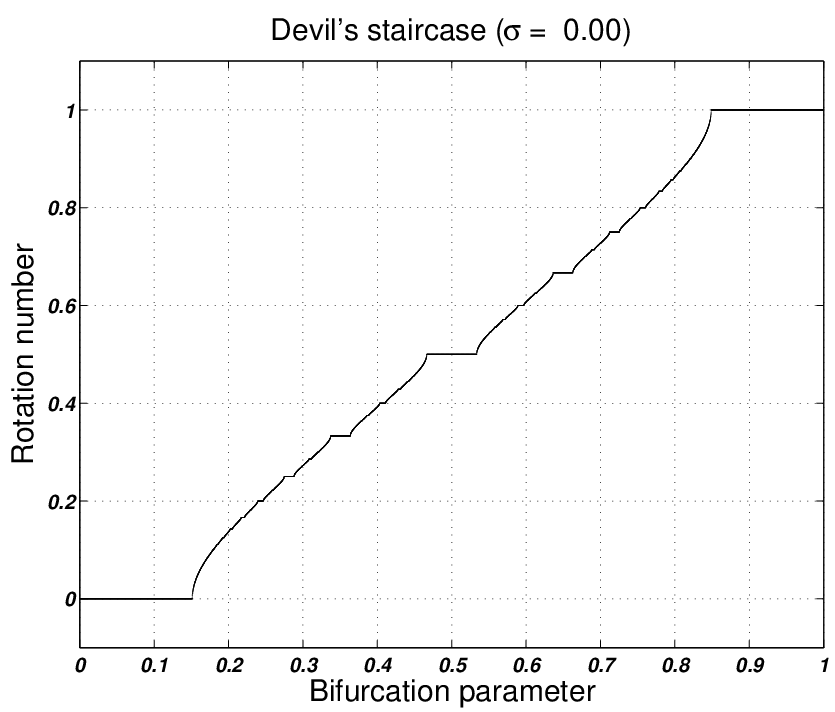
Proposition 9.4

\rho_{a}=\int_{\mathbb{R}/\mathbb{Z}}\mathbb{E}(\delta(x;\omega))d\mu_{a}(s)\qquad\nu^{\infty}-a.s.

(44)

where $\mathbb{E}$ is the expectation operator. The right hand side of (44) is independent of $x$ and is a smooth and nondecreasing function of $a$ .

Proof. Consider the Birkhoff sum in equation (43)

\frac{f_{a}^{k}(x;\omega)-x}{k}=\frac{1}{k}\sum_{i=0}^{k-1}\delta_{a}\circ S^{i}(s;\omega).

By Birkhoff’s ergodic theorem,

	$\displaystyle\lim_{k\to\infty}\frac{f_{a}^{k}(x;\omega)-x}{k}$	$\displaystyle=\int_{\mathbb{R}/\mathbb{Z}}\int_{\Omega}\beta_{a}(s;\omega)\mu_{a}(ds)\nu^{\infty}(d\omega)\qquad\mu_{a}\times\nu^{\infty}-a.s.$
		$\displaystyle=\int_{\mathbb{R}/\mathbb{Z}}\mathbb{E}(\beta_{a}(s;\omega))\mu_{a}(ds)\qquad\mu_{a}\times\nu^{\infty}-a.s.$		(45)

The fact that the rotation number when it exist is independent of the initial point, see (9.3), implies that this equality holds for all $x$ and $\nu^{\infty}-a.s.$ .

Write $a\mapsto h(a)$ for the right hand side of (44). Smoothness of $h$ follows from smoothness of the stationary density $\phi_{a}$ and (45). Write the standard family as $R_{a}\circ f(.;\omega)$ where $f(.;\omega)$ is the random map $f(x;\omega)=x+\frac{\varepsilon}{2\pi}\sin(2\pi x)+\sigma\xi(\omega)$ and $R_{a}$ is the translation with coefficient $a$ . Then for $a_{1}<a_{2}$ and $k\geq 1$ , $(R_{a_{1}}\circ f(.;\omega))^{k}<(R_{a_{2}}\circ f(.;\omega))^{k}$ and thus,

\rho_{a_{1}}=\lim_{k\to\infty}\frac{(R_{a_{1}}\circ f(.;\omega))^{k}-Id}{k}\leq\lim_{k\to\infty}\frac{(R_{a_{2}}\circ f(.;\omega))^{k}-Id}{k}=\rho_{a_{2}}.

$\square$

9.2 Random unimodal maps

This section is devoted to the investigation of the randomized version of the logistic family

f_{a}(x;\omega)=(a+\sigma\omega)x(1-x).

(46)

on $[0,1]$ . The random parameter $\omega$ be chosen from a uniform distribution on $\Delta=[-1,1]$ . Throughout this section we will assume that

a+\sigma\omega\in(1,4),

(47)

for all $\omega\in\Delta$ . As a consequence, the interval $[0,1]$ is mapped into itself by each map $x\mapsto f_{a}(x;\omega)$ and the fixed point at the origin is repelling. Any stationary measure will therefore have support contained in $(0,1)$ . We will demonstrate that there is only one stationary measure.

Proposition 9.5

The random logistic map $f_{a}$ has a unique stationary measure.

Proof. We collect some facts from unimodal dynamics needed in the sequel of the proof. The following facts hold for unimodal maps with negative Schwarzian derivative such as the logistic map $x\mapsto ax(1-x)$ . By Guckenheimer’s theorem, see [42, Theorem III.4.1], $x\mapsto ax(1-x)$ possesses a unique attractor $\Lambda_{a}$ . The attractor $\Lambda_{a}$ is either a periodic attractor, a solenoidal attractor, or a finite union of intervals on which the map acts transitively. In all cases, the omega-limit set of the critical point $c$ (with $c=\frac{1}{2}$ for the logistic map) is contained in $\Lambda_{a}$ . In fact, if $\Lambda_{a}$ is not a periodic attractor, then $c$ is contained in $\Lambda_{a}$ . It follows from a result of Misiurewicz, see [42, Theorem III.3.2], that the basin of attraction of $\Lambda_{a}$ is an open and dense subset of $(0,1)$ .

We will distinguish the following two cases.

Case (i):: There exists $\omega\in\Delta$ , so that $c\in\Lambda_{a+\sigma\omega}$ ,
Case (ii):: otherwise.

The two cases are treated separately.

Case (i): Write

W=\bigcap_{n\geq 0}\overline{\bigcup_{i\geq n}f^{i}_{a}(c;\Delta^{\mathbb{N}})}

for the omega-limit set of $c$ under all possible random iterations. Observe that $W$ is an invariant set. From the properties of the noise, $W$ consists of a finite union of intervals. Note that $c\in W$ , so that $W$ equals the closure of the positive orbit $\overline{\bigcup_{i\geq 0}f^{i}_{a}(c;\Delta^{\mathbb{N}})}$ of $c$ under all possible random iterations. We will prove that for each $x\in(0,1)$ , $y\in W$ and $\varepsilon>0$ , there exist $n>0$ and $\bar{{\boldsymbol{\omega}}}\in\Delta^{\mathbb{N}}$ with the property that

|f^{n}_{a}(x;\bar{{\boldsymbol{\omega}}})-y|<\varepsilon.

(48)

This implies the $W$ is the unique minimal invariant set, which in turn implies the theorem in the first case.

Fix $x\in(0,1)$ , $y\in W$ , $\varepsilon>0$ . From the construction of $W$ , there exist ${\boldsymbol{\omega}}_{1}\in\Delta^{\mathbb{N}}$ , $i>0$ , so that $|f^{i}_{a}(c;{\boldsymbol{\omega}}_{1})-y|<\varepsilon$ . By continuity of $x\mapsto f^{i}_{a}(x;{\boldsymbol{\omega}}_{1})$ , the same holds with $c$ replaced by a point from a $\delta$ neighborhood of $c$ for some $\delta>0$ . We need to establish the existence of $\hat{{\boldsymbol{\omega}}}\in\Delta^{\mathbb{N}}$ and $j>0$ so that $|f^{j}_{a}(x;\hat{{\boldsymbol{\omega}}})-c|<\delta$ . Let $\omega_{2}\in\Delta$ be such that $c\in\Lambda_{a+\sigma\omega_{2}}$ . Since the basin of attraction of $\Lambda_{a+\sigma\omega_{2}}$ is open and dense, there exists $\omega_{3}\in\Delta$ with $x_{1}=f_{a}(x;\omega_{3})$ contained in the basin of attraction of $\Lambda_{a+\sigma\omega_{2}}$ . For $i$ large, $x_{i}=f^{i-1}_{a}(x_{1};\omega_{2},\omega_{2},\cdots)$ is as close as desired to $\Lambda_{a+\sigma\omega_{2}}$ . If $\Lambda_{a+\sigma\omega_{2}}$ is a finite union of intervals, we get that $x_{i}$ is contained in $\Lambda_{a+\sigma\omega_{2}}$ for large enough $i$ . As inverse images of $c$ for $x\mapsto f_{a}(x;\omega_{2})$ are dense in $\Lambda_{a+\sigma\omega_{2}}$ , one deduces that there exist ${\boldsymbol{\omega}}_{4}\in\Delta^{\mathbb{N}}$ and $k>0$ so that $f^{k}_{a}(x_{i+1};{\boldsymbol{\omega}}_{4})$ lies in a $\delta$ neighborhood of $c$ . Indeed, if $\Lambda_{a+\sigma\omega_{2}}$ is a finite union of intervals, then we find $\omega_{5}$ with $x_{i+1}=f(x_{i};\omega_{5})$ equal to an inverse image of $c$ . If $\Lambda_{a+\sigma\omega_{2}}$ is a solenoidal attractor, then $x\mapsto f_{a}(x;\omega_{2})$ is infinitely renormalizable. In this case one can use ${\boldsymbol{\omega}}_{4}=(\omega_{2},\omega_{2},\cdots)$ . Also for a periodic attractor $\Lambda_{a+\sigma\omega_{2}}$ containing $c$ one uses ${\boldsymbol{\omega}}_{4}=(\omega_{2},\omega_{2},\cdots)$ .

Case (ii): By Guckenheimer’s theorem, $x\mapsto f_{a}(x;\omega)$ possesses a unique periodic attractor for each $\omega\in\Delta$ . Write $V$ for the the union of $\Lambda_{a+\sigma\omega}$ over $\omega\in\Delta$ . Define

W=\overline{\bigcup_{i\geq 0}f^{i}_{a}(V;\Delta^{\mathbb{N}})}.

This is clearly an invariant set. Note that we do not claim that $c$ is outside of $W$ . Arguments as before prove (48) with this definition of $W$ : for suitable noise one finds an orbit starting at $x$ that approaches a point in $V$ and then with further iterates approaches $y\in W$ . $\square$

Remark 9.6

The above proof applies to show that a random unimodal map $g(x;\omega)$ with negative Schwarzian derivative for each $\omega$ (the invoked theorem by Guckenheimer is true for these maps) has a unique stationary measure.

Perturbing away from the deterministic logistic family one sees that both random saddle node bifurcations and random homoclinic bifurcations occur in the random logistic family $\{f_{a}\}$ for small noise levels. Typically one can expect the following scenario. We start by recalling some facts concerning the dynamics of the deterministic map $f_{a}(\cdot;0)$ . The map $f_{a}(\cdot;0)$ is called renormalizable if there exists an interval $I$ and a positive integer $q$ , so that $f_{a}^{q}(I;0)\subset I$ . Let $[a_{-}.a_{+}]$ be a maximal interval so that $f_{a}(\cdot;0)$ is renormalizable for $a\in[a_{-},a_{+}]$ with $q$ constant. Then $f_{a}$ undergoes a saddle node bifurcation at $a=a_{-}$ involving a periodic orbit of period $q$ . At $a=a_{+}$ , $f_{a}$ undergoes a homoclinic bifurcation, where an iterate of $f_{a}$ maps the critical point onto a periodic orbit of period $q$ . For small noise levels (i.e. $\sigma$ small) one expects a random saddle node bifurcation near $a=a_{-}$ and a random homoclinic bifurcation near $a=a_{+}$ . Figure 6 illustrates this by computing Birkhoff averages for the logistic family and the random logistic family. See [32] for explanations of the computations for the logistic family.

Appendix A Representations of discrete Markov processes

In this appendix we explore the relation between random maps and discrete Markov processes given by stochastic transition functions. The random maps considered in this paper depend on random parameters, where the number of random parameters equals the dimension $n$ of the state space $\mathcal{M}$ . Proposition A.1 gives a wide class of Markov processes that can be represented by random maps by $n$ random parameters. The Markov process given by random maps depending on a larger number of random parameters (or even given by some measure on the space of maps) can be represented by random maps with $n$ random parameters.

Iterating a random map involves more random parameters obtained by independent draws at each iterate. By means of an example we explain how random maps with a smaller number of random parameters may be brought into the context of this paper. Consider the delayed logistic map $x_{n+1}=\mu x_{n}(1-x_{n-1})$ . Let $y_{n+1}=x_{n}$ . This defines a dynamical system $(x_{n+1},y_{n+1})=(\mu x_{n}(1-y_{n}),x_{n})$ . Assume now that $\mu$ is a random parameter varying in some interval with some distribution. This yields a random map

f(x,y;\mu)=(\mu x(1-y),x).

The derivative $Df$ is singular along $x=0$ . As $\mu$ is a single random parameter, this random diffeomorphism does not fit into the context considered in this paper. Considering two iterates gives two independent draws $(\mu,\nu)$ of the random parameter (that is, random parameters taken from a square) and yields the random map

f^{2}(x,y;\mu,\nu)=(\mu x(1-y),\nu\mu x(1-x)(1-y)).

If $x$ and $y$ stay away from $0$ and $1$ , the map and the dependence of $(\mu,\nu)$ are injective. The second iterate of the delayed logistic map with bounded parametric noise fulfills the assumptions in this paper.

There are other examples of maps with parametric noise that cannot be made to fulfill the assumptions used in this paper. For instance, random maps $f(x;\omega)=x+(x-\omega)^{2}$ with random $\omega$ from an interval, fail to satisfy the injectivity assumption of $\omega\mapsto f(x;\omega)$ . If $\omega$ is chosen from a uniform distribution, then the density of the transition function will not be bounded. Figure 7 indicates a random boundary bifurcation for a similar random map.

Consider discrete Markov processes given by transition functions $P(x,\cdot)$ . The following properties hold.

: For fixed $A\in{\cal B}$ , $x\mapsto P(x,A)$ is measurable.
: For fixed $x\in{\mathbb{R}}^{n}$ , $P(x,\cdot)$ is a probability measure.

Denote by $y\mapsto k(x,y)$ the density of $P(x,\cdot)$ . Write $U_{x}$ for the support of $k(x,\cdot)$ and let $U=\displaystyle{\cup_{x}}\left(\{x\}\times U_{x}\right)$ . Assume that $U_{x}$ is diffeomorphic to the closed unit ball $\Delta$ in ${\mathbb{R}}^{n}$ and varies smoothly with $x$ . We will assume that $y\mapsto k(x,y)$ depends smoothly on $(x,y)\in U$ , meaning that $k$ can be extended to a smooth function defined on an open neighborhood of $U$ . Under these conditions we will construct a representation by a finitely parameterized family of endomorphisms. That is, we will construct a family of endomorphisms $\{f_{\mu}\}$ on ${\mathbb{R}}^{n}$ , with parameters $\mu$ from an $n$ dimensional ball, and a measure $\nu$ on the parameter space so that $P(x,A)$ equals $\nu\{\mu\in\Delta\;|\;f_{\mu}(x)\in A\}$ . A corresponding result holds for discrete Markov processes with noise from an $n$ -dimensional box, see [11, Appendix D]. See [36] for a discussion of the existence of representations by sets of measurable or continuous maps. The paper [47] contains a result on representations by endomorphisms, under the assumption of unbounded noise.

Proposition A.1

There is a family of endomorphisms $f_{\mu}$ , $\mu\in\Delta$ , and a measure $\nu$ on $\Delta$ with smooth strictly positive density, so that

1.

$(x,\mu)\mapsto f_{\mu}(x)$ is smooth,
2.

for each $x\in\mathcal{M}$ , $\mu\mapsto f_{\mu}(x)$ is injective,
3.

$P(x,A)=\nu(\mu\in\Delta\;|\;f_{\mu}(x)\in A)$ .

Proof. We follow the arguments in [11], combined with the use of polar coordinates to map the unit ball $\Delta$ to $[0,1]^{n}$ . Let $\psi_{x}:V_{x}\to\Delta$ be a diffeomorphism, depending smoothly on $x$ , from the support $V_{x}$ of $y\mapsto k(x,y)$ to the unit ball. Consider polar coordinates $\chi:[0,1]^{n}\to\Delta$ on the unit ball,

\chi(\xi_{1},\ldots,\xi_{n})=\xi_{1}\left(\begin{array}[]{c}\cos(\pi\xi_{2})\\ \sin(\pi\xi_{2})\cos(\pi\xi_{3})\\ \vdots\\ \sin(\pi\xi_{2})\cdots\sin(\pi\xi_{n-1})\cos(2\pi\xi_{n})\\ \sin(\pi\xi_{2})\cdots\sin(\pi\xi_{n-1})\sin(2\pi\xi_{n})\end{array}\right).

For $\xi\in[0,1]^{n}$ , define sets $B_{i}(\xi)$ , $0\leq i\leq n$ , by

B_{i}(\xi)=\prod_{j=1}^{i}[0,\xi_{j}]\times\prod_{j=i+1}^{n}[0,1].

Write $C_{i}(\xi)=\psi_{x}^{-1}\chi^{-1}(B_{i}(\xi))$ and let $\omega=(\omega_{1},\ldots,\omega_{n})$ be given by

\omega_{i}=\int_{C_{i}(\xi)}k(x,y)dm(y)\left/\int_{C_{i-1}(\xi)}k(x,y)dm(y)\right..

Since $k>0$ , $\omega=\Theta(\xi)$ gives a 1-1 correspondence. Let $\eta_{i}=\int_{C_{i}(\xi)}dm(y)\left/\int_{C_{i-1}(\xi)}dm(y)\right.$ . Here $\eta=\Psi(\xi)$ is a 1-1 correspondence. The correspondence $\omega\to\eta$ is a smooth diffeomorphism as $k$ is smooth and strictly positive. Then

f_{\mu}(x)=\psi_{x}\chi\Psi^{-1}\Theta\chi^{-1}(\mu).

gives the required smooth random maps. $\square$

For discrete Markov processes on a circle there is an easy necessary and sufficient condition on the transition maps for a representation by random diffeomorphisms.

Proposition A.2

Let $\mathcal{M}$ be the circle endowed with Lebesgue measure. Write $V_{x}=[l_{-}(x),l_{+}(x)]$ . There is a representation by random smooth diffeomorphisms if and only if

-k(x,l_{-}(x))l_{-}^{\prime}(x)+\int_{l_{-}(x)}^{z}\frac{\partial}{\partial x}k(x,y)dy\neq 0

for $z\in V_{x}$ .

Proof. The construction of the representation by random smooth maps proceeds as follows. For $\xi\in[0,1]$ , write $C(\xi)=[l_{-}(x),l_{-}(x)+\xi(l_{+}(x)-l_{-}(x))]$ and let

\omega=\int_{C(\xi)}k(x,y)dy.

Since $k>0$ , the map $\Theta$ , $\Theta(\xi)=\omega$ , is a diffeomorphism. The representation by random diffeomorphisms is given through

f_{\omega}(x)=l_{-}(x)+\Theta^{-1}(\omega)(l_{+}(x)-l_{-}(x)).

Note that for fixed $\omega$ ,

\frac{d}{dx}\int_{[l_{-}(x),f_{\omega}(x)]}k(x,y)dy=0.

(49)

With, say, $l_{-}<f_{\omega}$ , (49) yields

-k(x,l_{-}(x))l_{-}^{\prime}(x)+k(x,f_{\omega}(x))f_{\omega}^{\prime}(x)+\int_{l_{-}(x)}^{f_{\omega}(x)}\frac{\partial}{\partial x}k(x,y)dy=0.

Hence $f_{\omega}^{\prime}(x)=0$ precisely if $-k(x,l_{-}(x))l_{-}^{\prime}(x)+\int_{l_{-}(x)}^{f_{\omega}(x)}\frac{\partial}{\partial x}k(x,y)dy=0$ . $\square$

Appendix B Regularity of solutions of integral equations

In a number of places in this paper eigenvalue equations $L_{a}\phi=\lambda\phi$ for the transfer operator $L_{a}$ arise. As $L_{a}$ depends only $C^{1}$ on $a$ , a direct application of the implicit function theorem as found e.g. in [10, 15] yields only weak regularity properties of the solutions.

The following remark is a variant of Proposition 4.1. It allows an application of [13, Proposition 3.6.1] to show that eigenvectors and eigenvalues of $L_{a}$ , in the case of simple eigenvalues, vary smoothly with $a$ .

Remark B.1

For $a\in I$ , $a\mapsto L_{a}$ is a $C^{r+1}$ map from $I$ into ${\cal L}(C^{k+r}(\mathcal{M}),C^{k}(\mathcal{M}))$ , the space of bounded linear maps from $C^{k+r}(\mathcal{M})$ into $C^{k}(\mathcal{M})$ .

We include in this appendix an alternative route to obtain such smoothness, as introduction to the more involved reasoning in Section 6.

Given is $L_{a_{0}}\phi_{a_{0}}=\lambda_{a_{0}}\phi_{a_{0}}$ with $L_{a}$ acting for $a$ near $a_{0}$ on $C^{k}(\mathcal{M})$ (here we are considering complex valued functions). Similarly we can consider $L_{a}$ acting on $C^{k}_{0}(W)$ for an isolating neighborhood $W$ . Assume that $\lambda_{a_{0}}$ is an isolated eigenvalue of $L_{a_{0}}$ . Denote by $E$ the span of $\phi_{a_{0}}$ and let $F^{k}(W)$ be a complement of $E$ in $C^{k}(\mathcal{M})$ . Consider functions $\phi_{a}=\phi_{a_{0}}+\psi_{a}$ with $\psi_{a}\in F^{k}(\mathcal{M})$ . We wish to solve $L_{a}\phi_{a}=\lambda_{a}\phi_{a}$ . Let $P$ be the projection to $E$ along $F^{k}(\mathcal{M})$ . Considering a second parameter $\lambda$ , $L_{a}\phi_{a}=\lambda\phi_{a}$ decomposes as

\left\{\begin{array}[]{lcl}(I-P)L_{a}(\phi_{a_{0}}+\psi_{a})&=&\lambda\psi_{a},\\ PL_{a}(\phi_{a_{0}}+\psi_{a})&=&\lambda\phi_{a_{0}}.\end{array}\right.

The top equation can be solved for $\psi_{a}$ as a function of $\lambda$ and $a$ for $a$ near $a_{0}$ and $\lambda$ near $\lambda_{a_{0}}$ . In fact, by the Fredholm alternative, $\psi_{a}=\left((I-P)L_{a}-\lambda I\right)^{-1}\left((I-P)L_{a}\phi_{a_{0}}\right)$ . Putting this into the bottom equation yields a single equation for $\lambda$ . Note that for stationary measures, $\lambda=1$ automatically solves this equation, compare the proof of Theorem 1.10 in Section 4.

Write the top equation as a fixed point equation $T_{\alpha}\psi_{\alpha}=\psi_{\alpha}$ with parameters $\alpha$ . The map $T_{\alpha}$ is a compact linear map mapping $F^{k}(\mathcal{M})$ into $F^{k+1}(\mathcal{M})$ , compare the proof of Proposition 2.3.

Lemma B.2

If $(x,a)\mapsto\psi_{a}(x)$ is $C^{k}$ , then $(x,a)\mapsto T_{a}\psi_{a}(x)$ is $C^{k+1}$ .

Proof. See Section 4. $\square$

Proposition B.3

Consider the integral equation $T_{\alpha}\psi_{\alpha}=\psi_{\alpha}$ with $T_{\alpha}$ as above. The fixed point $x\mapsto\psi_{\alpha}(x)$ is smooth jointly in $x,\alpha$ .

Proof. Given is a unique fixed point $\psi_{\alpha}$ depending continuously on $\alpha$ . Formally differentiating $T_{\alpha}\psi_{\alpha}=\psi_{\alpha}$ with respect to $\alpha$ gives

\frac{\partial}{\partial\alpha}\left(T_{\alpha}\psi_{\alpha}(x)\right)=\frac{\partial}{\partial\alpha}T_{\alpha}\psi_{\alpha}(x)+T_{\alpha}\frac{\partial}{\partial\alpha}\psi_{\alpha}(x)=\frac{\partial}{\partial\alpha}\psi_{\alpha}(x).

So $\frac{\partial}{\partial\alpha}\psi_{\alpha}$ should be the solution $M_{\alpha}$ of $\frac{\partial}{\partial\alpha}T_{\alpha}\psi_{\alpha}(x)+T_{\alpha}M_{\alpha}(x)=M_{\alpha}(x)$ . That is,

M_{\alpha}=(I-T_{\alpha})^{-1}\frac{\partial}{\partial\alpha}T_{\alpha}\psi_{\alpha}.

(50)

By the Fredholm alternative [38], $I-T_{\alpha}$ is invertible on $F^{k}(\mathcal{M})$ . The right hand side of (50) is therefore a continuous function. To establish that $M_{\alpha}$ is the derivative $\frac{\partial}{\partial\alpha}\psi_{\alpha}$ , we must show $|\psi_{\alpha+h}(x)-\psi_{\alpha}(x)-M_{\alpha}(x)h|=o(|h|)$ as $h\to 0$ (compare the proof of the implicit function theorem in e.g. [10] or [15]). Write $\gamma_{\alpha}(x)=\psi_{\alpha+h}(x)-\psi_{\alpha}(x)$ . Now

	$\displaystyle\gamma_{\alpha}(x)$	$\displaystyle=$	$\displaystyle T_{\alpha+h}(\psi_{\alpha}+\gamma_{\alpha})(x)-T_{\alpha}(\psi_{\alpha})(x)$		(51)
		$\displaystyle=$	$\displaystyle T_{\alpha}\gamma_{\alpha}(x)+\frac{\partial}{\partial\alpha}T_{\alpha}\psi_{\alpha}(x)h+R(x),$		(51)

where $R(x)=T_{\alpha+h}(\psi_{\alpha}+\gamma_{\alpha})(x)-T_{\alpha}(\psi_{\alpha})(x)-T_{\alpha}\gamma_{\alpha}(x)-\frac{\partial}{\partial\alpha}T_{\alpha}\psi_{\alpha}(x)h$ . Since $(\psi,\alpha)\mapsto T_{\alpha}(\psi)$ is differentiable, for any $\epsilon>0$ there is $\delta>0$ with $|R|<\epsilon(|\gamma_{\alpha}|+|h|)$ if $|\gamma_{\alpha}|,|h|<\delta$ . Since $\gamma_{\alpha}$ is continuous in $h$ , we may further restrict $\delta$ so that this estimate on $|R|$ holds for $|h|<\delta$ . From (51) we get $\gamma_{\alpha}=(I-T_{\alpha})^{-1}(\frac{\partial}{\partial\alpha}T_{\alpha}\psi_{\alpha}h+R)$ so that $|\gamma_{\alpha}|<C|h|$ for some $C$ , if $|h|<\delta$ . This implies $|R|<\epsilon(1+C)|h|$ for $|h|<\delta$ . As

(I-T_{\alpha})(\gamma_{\alpha}-M_{\alpha}h)=R

(from (50) we get $(I-T_{\alpha})M_{\alpha}=\frac{\partial}{\partial\alpha}T_{\alpha}\psi_{\alpha}$ ), we derive $|\gamma_{\alpha}(x)-M_{\alpha}(x)h|<K\epsilon|h|$ for some $K>0$ , if $|h|<\delta$ . This proves that $M_{\alpha}$ equals the partial derivative $\frac{\partial}{\partial\alpha}\psi_{\alpha}$ .

Higher order derivatives are treated by induction. Assume that $(x,\alpha)\mapsto\psi_{\alpha}(x)$ has been shown to be $C^{j}$ . By Lemma B.2, $(x,\alpha)\mapsto T_{\alpha}\psi_{\alpha}(x)$ is $C^{j+1}$ . So $D\psi_{\alpha}=D(T_{\alpha}\psi_{\alpha})$ is $C^{j}$ . As $(I-T_{\alpha})^{-1}$ maps $F^{j}(\mathcal{M})$ to $F^{j}(\mathcal{M})$ , the right hand side of (50) is a $C^{j}$ function. The above reasoning shows that $M_{\alpha}=\frac{\partial}{\partial\alpha}\psi_{\alpha}$ . Therefore $\frac{\partial}{\partial\alpha}\psi_{\alpha}$ is $C^{j}$ , so that $(x,\alpha)\mapsto\psi_{\alpha}(x)$ is $C^{j+1}$ . $\square$

References

[1] R. Abraham, J.E. Marsden, T. Ratiu, Manifolds, tensor analysis, and applications, Addison-Wesley Publishing Company, 1983.
[2] J.F. Alves, V. Araújo, Random perturbations of nonuniformly expanding maps, Astérisque 286 (2003), 25–62.
[3] J.F. Alves, V. Araújo, C.H. Vásquez, Random perturbations of diffeomorphisms with dominated splitting, preprint CMUP, 2004.
[4] V. Araújo, Attractors and time averages for random maps, Ann. Inst. H. Poincaré Anal. Non Linéaire 17 (2000), 307–369.
[5] L. Arnold, Random Dynamical Systems, Springer-Verlag, 1998.
[6] V. Baladi, Positive transfer operators and decay of correlations, World Scientific, 2000.
[7] V. Baladi, M. Viana, Strong stochastic stability and rate of mixing for unimodal maps, Annales Scientifiques de l’École Normale Supérieure Sér. 4 29 (1996), 483–517.
[8] V. Baladi, L.-S. Young, On the spectra of randomly perturbed expanding maps, Comm. Math. Phys. 156 (1993), 355–385.
[9] V. Baladi, L.-S. Young, Erratum: ”On the spectra of randomly perturbed expanding maps”, Comm. Math. Phys. 166 (1994), 219–220.
[10] M.S. Berger, Nonlinearity and functional analysis, Academic Press, 1977.
[11] C. Bonatti, L.J. Diaz, M. Viana, Dynamics beyond uniform hyperbolicity, Springer-Verlag, 2005.
[12] S. Brassesco, E. Olivieri, M.E. Vares, Couplings and asymptotic exponentiality of exit times, J. Statist. Phys. 93 (1998), 393–404.
[13] B. Buffoni, J. Toland, Analytic theory of global bifurcation, Princeton University Press, 2003.
[14] N. Chernov, R. Markarian, S. Troubetzkoy, Conditionally invariant measures for Anosov maps with small holes, Ergodic Theory Dynam. Systems 18 (1998), 1049–1073.
[15] S.-N. Chow, J.K. Hale, Methods of bifurcation theory, Springer-Verlag, 1982.
[16] F. Colonius, W. Kliemann, The dynamics of control, Birkhäuser, 2000.
[17] F. Colonius, T. Gayer, W. Kliemann, Near invariance for Markov diffusion systems, preprint.
[18] M.V. Day, On the exponential exit law in the small parameter exit problem, Stochastics 8 (1983), 297–323.
[19] M. Dellnitz, O. Junge, On the approximation of complicated dynamical behavior, SIAM J. Numer. Anal. 36 (1999), 491–515.
[20] S. Doi, J. Inoue, S. Kumagai, Spectral analysis of stochastic phase lockings and stochastic bifurcations in the sinusoidally forced van der Pol oscillator with additive noise, J. Statist. Phys. 90 (1998), 1107–1127.
[21] J.L. Doob, Stochastic Processes, John Wiley & Sons, 1953.
[22] J.-P. Eckmann, L. Thomas, P. Wittwer, Intermittency in the presence of noise, J. Phys. A 14 (1981), 3153–3168.
[23] P.A. Ferrari, H. Kesten, S. Martinez, P. Picco, Existence of quasi-stationary distributions. A renewal dynamical approach, Ann. Probab. 23 (1995), 501–521.
[24] M.K. Fort, Points of continuity of semi-continuous functions, Publ. Math. Debrecen 2 (1951), 100–102.
[25] M.I. Freidlin, A.D. Wentzell, Random perturbations of dynamical systems, Springer-Verlag, 1984.
[26] T. Gayer, On Markov chains and the spectra of the corresponding Frobenius-Perron operators, Stoch. Dyn. 1 (2001), 477–491.
[27] T. Gayer, Control sets and their boundaries under parameter variation, J. Differential Equations 201 (2004), 177–200.
[28] C. Grebogi, E. Ott, F. Romeiras, J.A. Yorke, Critical exponents for crisis-induced intermittency, Phys. Rev. A 36 (1987), 5365–5380.
[29] M.R. Herman, Sur la conjugaison différentiable des difféomorphismes du cercle à des rotations, Publications mathématique de l’I.H.É.S. 49 (1979), 5–233.
[30] J.E. Hirsch, B.A. Huberman, D.J. Scalapino, Theory of intermittency, Physical Review A 25 (1982), 519–532.
[31] M.W. Hirsch, Differential topology, Springer-Verlag, 1976.
[32] A.J. Homburg, T. Young, Intermittency in families of unimodal maps, Ergodic Theory Dynam. Systems 22 (2002), 203–225.
[33] A.J. Homburg, T. Young, Intermittency and Jakobson’s theorem near saddle-node bifurcations, preprint.
[34] A.J. Homburg, T. Young, Hard bifurcations in dynamical systems with bounded random perturbations, preprint.
[35] T. Kato, Perturbation theory for linear operators, Springer-Verlag, 1966.
[36] Y. Kifer, Ergodic theory of random transformations, Birkhäuser, 1986.
[37] Y. Kifer, Random perturbations of dynamical systems, Birkhäuser, 1988.
[38] E. Kreyszig, Introductory functional analysis with applications, John Wiley & Sons, 1978.
[39] A. Lasota, M.C. Mackey, Chaos, fractals and noise, Springer-Verlag, 1994.
[40] J.B. Lasserre, C.E.M. Pearce, On the existence of a quasistationary measure for a Markov chain, Ann. Probab. 29, 427–446.
[41] R.S. MacKay, An extension of Zeeman’s notion of structural stability to noninvertible maps, Phys. D 52 (1991), 246–253.
[42] W. de Melo, S. van Strien, One-dimensional dynamics, Springer-Verlag, 1993.
[43] J.W. Milnor, Dynamics: introductory lectures, http://www.math.sunysb.edu/~jack/DYNOTES/
[44] G. Pianigiani, Conditionally invariant measures and exponential decay, J. Math. Anal. Appl. 82 (1981), 75–88.
[45] G. Pianigiani, J.A. Yorke, Expanding maps on sets which are almost invariant. Decay and chaos, Trans. Amer. Math. Soc. 252 (1979), 351–366.
[46] Y. Pomeau, P. Manneville, Intermittent transition to turbulence in dissipative dynamical systems, Comm. Math. Phys. 74 (1980), 189–197.
[47] A.N. Quas, On representations of Markov chains by random smooth maps, Bull. London Math. Soc. 23 (1991), 487–492.
[48] D. Ruelle, Small random perturbations of dynamical systems and the definition of attractors, Comm. Math. Phys. 82 (1982), 137–151.
[49] D. Ruelle, An extension of the theory of Fredholm determinants, Inst. Hautes Études Sci. Publ.Math. 72 (1990), 175–193.
[50] H.H. Schaefer, Banach lattices and positive operators, Springer-Verlag, 1974.
[51] M. Viana, Stochastic dynamics of deterministic systems, Col. Bras. de Matemática, 1997.
[52] K. Yosida, Functional Analysis, Springer-Verlag, 1980.
[53] L.-S. Young, Stochastic stability of hyperbolic attractors, Ergodic Theory Dynam. Systems 6 (1986), 311–319.
[54] E.C. Zeeman, Stability of dynamical systems, Nonlinearity 1 (1988), 115–155.

	$\displaystyle\lim_{h\to 0}\frac{1}{\|h\|}\int_{V_{x}\backslash(V_{x+h}\cap V_{x})}k(y,x)\psi(y)dy$	$\displaystyle=$	$\displaystyle\lim_{h\to 0}\frac{1}{\|h\|}\int_{[0,1]^{n-1}}\int_{H_{x}(y_{1})}^{H_{x+h}(y_{1})}k(y_{1},y_{2},x)\psi(y)dy_{2}dy_{1}$
		$\displaystyle=$	$\displaystyle\int_{[0,1]^{n-1}}\frac{\partial}{\partial x}H_{x}(y_{1})\frac{h}{\|h\|}k(y_{1},H_{x}(y_{1}),x)\psi(y_{1},H_{x}(y_{1}))dy_{1}$