Counting Rooted Trees :
The Universal Law $t(n)\,\sim\,C\rho^{-n}n^{-3/2}$ Thanks: We are greatly indebted to the referee for bringing up important questions, especially regarding the role of ${\sf Set}$ , that led us to thoroughly rework the paper.Thanks: The second and third authors would like to thank NSERC for support of this research.

Jason P. Bell Address: Department of Mathematics, Simon Fraser University,8888 University Dr., Burnaby, BC, V5A 1S6, Canada Email address: jpb@math.sfu.ca , Stanley N. Burris Address: Department of Pure Mathematics, University of Waterloo,Waterloo, Ontario, N2L 3G1, Canada Email address: snburris@thoralf.uwaterloo.ca URL: www.thoralf.uwaterloo.ca and Karen A. Yeats Address: Department of Mathematics and Statistics, Boston University, 111 Cummington St, Boston, MA 02215, USA Email address: kayeats@math.bu.edu

Date: July 27, 2006
Mathematics Subject Classifications: Primary 05C05; Secondary 05A16, 05C3 0, 30D05

Abstract.

Combinatorial classes ${\mathcal{T}}$ that are recursively defined using combinations of the standard multiset, sequence, directed cycle and cycle constructions, and their restrictions, have generating series ${\bf T}(z)$ with a positive radius of convergence; for most of these a simple test can be used to quickly show that the form of the asymptotics is the same as that for the class of rooted trees: $C\rho^{-n}n^{-3/2}$ , where $\rho$ is the radius of convergence of ${\bf T}$ .

1. Introduction

The class of rooted trees, perhaps with additional structure as in the planar case, is unique among the well studied classes of structures. It is so easy to find endless possibilities for defining interesting subclasses as the fixpoint of a class construction, where the constructions used are combinations of a few standard constructions like sequence, multiset and add-a-root. This fortunate situation is based on a simple reconstruction property: removing the root from a tree gives a collection of trees (called a forest); and it is trivial to reconstruct the original tree from the forest (by adding a root).

Since we will be frequently referring to rooted trees, and rarely to free (i.e., unrooted) trees, from now on we will assume, unless the context says otherwise, that the word ‘tree’ means ‘rooted tree’.

1.1. Cayley’s fundamental equation for trees

Cayley [5] initiated the tree investigations¹¹ 1 This was in the context of an algorithm for expanding partial differential operators. Trees play an important role in the modern theory of differential equations and integration—see for example Butcher [3]. in 1857 when he presented the well known infinite product representation²² 2 This representation uses $t(n)$ to count the number of trees on $n$ vertices. Cayley actually used $t(n)$ to count the number of trees with $n$ edges, so his formula was ${\bf T}(z)\ =\ z\prod_{j\geq 1}\big(1-z^{j}\big)^{-t(j-1)}.$

{\bf T}(z)\ =\ z\prod_{j\geq 1}\big(1-z^{j}\big)^{-t(j)}\,.

Cayley used this to calculate $t(n)$ for $1\leq n\leq 13$ . More than a decade later ([7], [8], [10]) he used this method to give recursion procedures for finding the coefficients of generating functions for the chemical diagrams of certain families of compounds.

1.2. Pólya’s analysis of the generating series for trees

Following on Cayley’s work and further contributions by chemists, Pólya published his classic 1937 paper³³ 3 Republished in book form in [26]. that presents: (1) his group-theoretic approach to enumeration, and (2) the primary analytic technique to establish the asymptotics of recursively defined classes of trees. Let us review the latter as it has provided the paradigm for all subsequent investigations into generating series defined by recursion equations.

Let ${\bf T}(z)$ be the generating series for the class of all unlabelled trees. Pólya first converts Cayley’s equation to the form

{\bf T}(z)\ =\ z\cdot\exp\Big(\sum_{m\geq 1}{\bf T}(z^{m})/m\Big).

From this he quickly deduces that: the radius of convergence $\rho$ of ${\bf T}(z)$ is in $(0,1)$ and ${\bf T}(\rho)<\infty$ . He defines the bivariate function

{\bf E}(z,w):=ze^{w}\cdot\exp\Big(\sum_{m\geq 2}{\bf T}(z^{m})/m\Big),

giving the recursion equation ${\bf T}={\bf E}\big(z,{\bf T}\big)$ . Since ${\bf E}(z,w)$ is holomorphic in a neighborhood of ${\bf T}$ he can invoke the Implicit Function Theorem to show that a necessary condition for $z$ to be a dominant singularity, that is a singularity on the circle of convergence, of ${\bf T}$ is

{\bf E}_{w}\big(z,{\bf T}(z)\big)=1.

From this Pólya deduces that ${\bf T}$ has a unique dominant singularity, namely $z=\rho$ . Next, since ${\bf E}_{z}\big(\rho,{\bf T}(\rho)\big),\,{\bf E}_{ww}\big(\rho,{\bf T}(\rho)\big)\neq 0$ , the Weierstraß Preparation Theorem shows that $\rho$ is a square-root type singularity. Applying well known results derived from the Cauchy Integral Theorem

(1)

t(n)\ =\ \frac{1}{2\pi i}\int_{\mathcal{C}}\frac{{\bf T}(z)}{z^{n+1}}dz

one has the famous asymptotics

\begin{array}[]{l @{\quad} l}\boldsymbol{(\star)}&\qquad\qquad\qquad\qquad t(n)\ \sim\ C\rho^{-n}n^{-3/2}\end{array}

which occur so frequently in the study of recursively defined classes.

1.3. Subsequent developments

Bender ([1], 1974) proposed a general version of the Pólya result, but Canfield ([4], 1983) found a flaw in the proof, and proposed a more restricted version. Harary, Robinson and Schwenk ([17], 1975) gave a 20 step guideline on how to carry out a Pólya style analysis of a recursion equation. Meir and Moon ([21], 1989) made some further proposals on how to modify Bender’s approach; in particular it was found that the hypothesis that the coefficients of ${\bf E}$ be nonnegative was highly desirable, and covered a great number of important cases. This nonnegativity condition has continued to find favor, being used in Odlyzko’s survey paper [23] and in the forthcoming book [15] of Flajolet and Sedgewick. Odlyzko’s version seems to be a current standard—here it is (with minor corrections due to Flajolet and Sedgewick [15]).

Theorem 1 (Odlyzko [23], Theorem 10.6).

Suppose

(2)		$\displaystyle{\bf E}(z,w)$	$\displaystyle=$	$\displaystyle\sum_{i,j\geq 0}e_{ij}z^{i}w^{j}\quad\text{with }e_{00}=0,\,e_{01}<1,\,(\forall i,j)\,e_{ij}\geq 0$
(3)		$\displaystyle{\bf T}(z)$	$\displaystyle=$	$\displaystyle\sum_{i\geq 1}t_{i}z^{i}\quad\text{with }(\forall i)\,t_{i}\geq 0$

are such that

a

${\bf T}(z)$ is analytic at $x=0$
b

${\bf T}(z)={\bf E}\big(z,{\bf T}(z)\big)$
c

${\bf E}(z,w)$ is nonlinear in $w$
d

there are positive integers $i,j,k$ with $i<j<k$ such that

$\displaystyle t_{i},t_{j},t_{k}$ $\displaystyle>$ $\displaystyle 0$

$\displaystyle\gcd(j-i,k-i)$ $\displaystyle=$ $\displaystyle 1.$

Suppose furthermore that there exist $\delta,r,s>0$ such that

(e)

${\bf E}(z,w)$ is analytic in $|z|<r+\delta$ and $|w|<s+\delta$
(f)

${\bf E}(r,s)=s$
(g)

${\bf E}_{w}(r,s)=1$
(h)

${\bf E}_{z}(r,s)\neq 0$ and ${\bf E}_{ww}(r,s)\neq 0$ .

Then $r$ is the radius of convergence of ${\bf T}$ , ${\bf T}(r)=s$ , and as $n\rightarrow\infty$

t_{n}\ \sim\ \sqrt{\frac{r{\bf E}_{z}(r,s)}{2\pi{\bf E}_{ww}(r,s)}}\cdot r^{n}n^{-3/2}.

Remark 2.

As with Pólya’s original result, the asymptotics in these more general theorems follow from information gathered on the location and nature of the dominant singularities of ${\bf T}$ . It has become popular to require that the solution ${\bf T}$ have a unique dominant singularity—to guarantee this happens the above theorem has the hypothesis (d). One can achieve this with a weaker hypothesis, namely one only needs to require

\mbox{\rm(d${}^{\prime}$)}\quad\gcd\big(\{j-i:i<j\text{ and }t_{i},t_{j}>0\}\big)=1.

Actually, given the other hypotheses of Theorem 1, the condition (d^′) is necessary and sufficient that ${\bf T}$ have a unique dominant singularity.

The generalization of Pólya’s result that we find most convenient is given in Theorem 28. We will also adopt the condition that ${\bf E}$ have nonnegative coefficients, but point out that under this hypothesis the location of the dominant singularities is quite easy to determine. Consequently the unique singularity condition is not needed to determine the asymptotics.

For further remarks on previous variations and generalizations of the work of Pólya see $\lx@sectionsign\,$ 7. The condition that the ${\bf E}$ have nonnegative coefficients forces us to omit the ${\sf Set}$ operator from our list of standard combinatorial operators. There are a number of complications in trying to extend the results of this paper to recursion equations $w={\bf G}(z,w)$ where ${\bf G}$ has mixed signs appearing with its coefficients, including the problem of locating the dominant singularities of the solution. The situation with mixed signs is discussed in $\lx@sectionsign$ 6.

1.4. Goal of this paper

Aside from the proof details that show we do not need to require that the solution ${\bf T}$ have a unique dominant singularity, this paper is not about finding a better way of generalizing Pólya’s theorem on trees. Rather the paper is concerned with the ubiquity of the form $\boldsymbol{(\star)}$ of asymptotics that Pólya found for the recursively defined class of trees.⁴⁴ 4 The motivation for our work came when a colleague, upon seeing the asymptotics of Pólya for the first time, said “Surely the form $\boldsymbol{(\star)}$ hardly ever occurs! (when finding the asymptotics for the solution of an equation $w=\Theta(w)$ that recursively defines a class of trees)”. A quick examination of the literature, a few examples, and we were convinced that quite the opposite held, that almost any reasonable class of trees defined by a recursive equation that is nonlinear in $w$ would lead to an asymptotic law of Pólya’s form $\boldsymbol{(\star)}$ .

The goal of this paper is to exhibit a very large class of natural and easily recognizable operators $\Theta$ for which we can guarantee that a solution $w={\bf T}(z)$ to the recursion equation $w=\Theta(w)$ has coefficients that satisfy $\boldsymbol{(\star)}$ . By ‘easily recognizable’ we mean that you only have to look at the expression describing $\Theta$ —no further analysis is needed. This contrasts with the existing literature where one is expected to carry out some calculations to determine if the solution ${\bf T}$ will have certain properties. For example, in Odlyzko’s version, Theorem 1, there is a great deal of work to be done, starting with checking that the solution ${\bf T}$ is analytic at $z=0$ .

In the formal specification theory for combinatorial classes (see Flajolet and Sedgewick [15]) one starts with the binary operations of disjoint union and disjoint sum and adds unary constructions that transform a collection of objects (like trees) into a collection of objects (like forests). Such constructions are admissible if the generating series of the output class of the construction is completely determined by the generating series of the input class.

We want to show that a recursive specification using almost any combination of these constructions, and others that we will introduce, yield classes whose generating series have coefficients that obey the asymptotics $\boldsymbol{(\star)}$ of Pólya. It is indeed a universal law. The goal of this paper is to provide truly practical criteria (Theorem 75) to verify that many, if not most, of the common nonlinear recursion equations lead to $\boldsymbol{(\star)}$ . Here is a contrived example to which this theorem applies:

(4)

w\ =\ z\ +\ z{\sf MSet}\Big({\sf Seq}\big(\sum_{n\in{\sf Odd}}6^{n}w^{n}\big)\Big)\sum_{n\in{\sf Even}}(2^{n}+1)\big({\sf DCycle}_{{\sf Primes}}(w)\big)^{n}\,.

An easy application of Theorem 75 (see $\lx@sectionsign\,$ 4.29) tells us this particular recursion equation has a recursively defined solution ${\bf T}(z)$ with a positive radius of convergence, and the asymptotics for the coefficients $t_{n}$ have the form $\boldsymbol{(\star)}$ .

The results of this paper apply to any combinatorial situation described by a recursion equation of the type studied here. We put our focus on classes of trees because they are by far the most popular setting for such equations.

1.5. First definitions

We start with our basic notation for number systems, power series and open discs.

Definition 3.

a

${\mathbb{R}}$ is the set of reals; ${\mathbb{R}}^{\geq 0}$ is the set of nonnegative reals.
b

${\mathbb{P}}$ is the set of positive integers. ${\mathbb{N}}$ is the set of nonnegative integers.
c

${\mathbb{R}}^{\geq 0}[[z]]$ is the set of power series in $z$ with nonnegative coefficients.
d

$\rho_{\bf A}$ is the radius (of convergence) of the power series ${\bf A}$ .
e

For ${\bf A}\in{\mathbb{R}}^{\geq 0}[[z]]$ we write ${\bf A}\,=\,\sum_{n}a(n)z^{n}$ or ${\bf A}\,=\,\sum_{n}a_{n}z^{n}$ .
f

For $r>0$ and $z_{0}\in{\mathbb{C}}$ the open disc of radius $r$ about $z_{0}$ is ${\mathbb{D}}_{r}(z_{0})\,:=\,\{z:|z-z_{0}|<r\}$

1.6. Selecting the domain

We want to select a suitable collection of power series to work with when determining solutions $w={\bf T}$ of recursion equations $w=\Phi(w)$ . The intended application is that ${\bf T}$ be a generating series for some collection of combinatorial objects. Since generating series have nonnegative coefficients we naturally focus on series in ${\mathbb{R}}^{\geq 0}[[z]]$ .

There is one restriction that seems most desirable, namely to consider as generating functions only series whose constant term is 0. A generating series ${\bf T}$ has the coefficient $t(n)$ of $z^{n}$ counting (in some fashion) objects of size $n$ . It has become popular when working with combinatorial systems to admit a constant coefficient when it makes a result look simpler, for example with permutations we write ${\bf A}(z)=\exp\big({\bf Q}(z)\big)$ , where ${\bf A}(z)$ is the exponential generating series for permutations, and ${\bf Q}(z)$ the exponential generating series for cycles. ${\bf Q}(z)=\log\big(1/(1-z)\big)$ will have a constant term 0, but ${\bf A}(z)=1/(1-z)$ will have the constant term 1. Some authors like to introduce an ‘ideal’ object of size 0 to go along with this constant term.

There is a problem with this convention if one wants to look at compositions of operators. For example, suppose you wanted to look at sequences of permutations. The natural way to write the generating series would be to apply the sequence operator ${\sf Seq}$ to $1/(1-z)$ above, giving $\sum 1/(1-z)^{n}$ . Unfortunately this “series” has constant coefficient $=\infty$ , so we do not have an analytical function. The culprit is the constant 1 in ${\bf A}(z)$ . If we drop the 1, so that we are counting only ‘genuine’ permutations, the generating series for permutations is $z/(1-z)$ ; applying ${\sf Seq}$ to this gives $z/(1-2z)$ , an analytical function with radius of convergence 1/2.

Consequently in this paper we return to the older convention of having the constant term be 0, so that we are only counting ‘genuine’ objects.

Definition 4.

For ${\bf A}\in{\mathbb{R}}[[z]]$ we write ${\bf A}\unrhd 0$ to say that all coefficients $a_{i}$ of ${\bf A}$ are nonnegative. Likewise for ${\bf B}\in{\mathbb{R}}[[z,w]]$ we write ${\bf B}\unrhd 0$ to say all coefficients $b_{ij}$ are nonnegative. Let

a

${\mathbb{DOM}}[z]\,:=\,\{{\bf A}\in{\mathbb{R}}^{\geq 0}[[z]]:{\bf A}(0)=0\}$ , the set of power series ${\bf A}\unrhd 0$ with constant term $0$ ; and let
b

${\mathbb{DOM}}[z,w]\,:=\,\{{\bf E}\in{\mathbb{R}}^{\geq 0}[[z,w]]:{\bf E}(0,0)=0\},$ the set of power series ${\bf E}\unrhd 0$ with constant term $0$ . Members of this class are called elementary power series.⁵⁵ 5 We use the name elementary since a recursion equation of the form $w={\bf E}(z,w)$ is in the proper form to employ the tools of analysis that are presented in the next section.

When working with a member ${\bf E}\in{\mathbb{DOM}}[z,w]$ it will be convenient to use various series formats for writing ${\bf E}$ , namely

$\displaystyle{\bf E}(z,w)$	$\displaystyle=$	$\displaystyle\sum_{ij}e_{ij}z^{i}w^{j}$
$\displaystyle{\bf E}(z,w)$	$\displaystyle=$	$\displaystyle\sum_{j}{\bf E}_{j}(z)w^{j}$
$\displaystyle{\bf E}(z,w)$	$\displaystyle=$	$\displaystyle\sum_{j}\Big(\sum_{i}e_{ij}z^{i}\Big)w^{j}.$

This is permissible from a function-theoretic viewpoint since all coefficients $e_{ij}$ are nonnegative; for any given $z,w\geq 0$ the three formats converge to the same value (possibly infinity).

An immediate advantage of working with series having nonnegative coefficients is that the series is defined (possibly infinite) at its radius of convergence.

Lemma 5.

For ${\bf T}\,\in\,{\mathbb{DOM}}[z]$ one has ${\bf T}(\rho_{\bf T})\in[0,\infty]$ . Suppose ${\bf T}(\rho_{\bf T})\,\in\,(0,\infty)$ . Then $\rho_{\bf T}\,<\,\infty$ ; in particular ${\bf T}$ is not a polynomial. If furthermore ${\bf T}$ has integer coefficients then $\rho_{\bf T}\,<\,1$ .

2. The theoretical foundations

We want to show that the series ${\bf T}$ that are recursively defined as solutions to functional equations $w={\bf G}(z,w)$ are such that with remarkably frequency the asymptotics of the coefficients $t_{n}$ are given by $\boldsymbol{(\star)}$ . Our main results deal with the case that ${\bf G}(z,w)$ is holomorphic in a neighborhood of $(0,0)$ , and the expansion $\sum g_{ij}z^{i}w^{j}$ is such that all coefficients $g_{ij}$ are nonnegative. This covers most of the equations arising from combinations of the popular combinatorial operators like Sequence, MultiSet and Cycle.

The referee noted that we had omitted one popular construction, namely ${\sf Set}$ , and the various restrictions ${\sf Set}_{\mathbb{M}}$ of ${\sf Set}$ , and asked that we explain this omission. Although the equation $w=z+z{\sf Set}(w)$ has been successfully analyzed in [17], there are difficulties when one wishes to form composite operators involving ${\sf Set}$ . These difficulties arise from the fact that the resulting equation $w={\bf G}(z,w)$ has ${\bf G}$ with coefficients having mixed signs. A general discussion of the mixed signs case is given in $\lx@sectionsign$ 6.1 and a particular discussion of the ${\sf Set}$ operator in $\lx@sectionsign$ 6.2. Since the issue of mixed signs is so important we introduce the following abbreviations.

Definition 6.

A bivariate series ${\bf E}(z,w)$ and the associated functional equation $w={\bf E}(z,w)$ are nonnegative if the coefficients of ${\bf E}$ are nonnegative. A bivariate series ${\bf G}(z,w)$ and the associated functional equation $w={\bf G}(z,w)$ have mixed signs if some coefficients $g_{ij}$ are positive and some are negative.

To be able to locate the difficulties when working with mixed signs, and to set the stage for further research on this topic, we have put together an essentially complete outline of the steps we use to prove that a solution ${\bf T}$ to a functional equation $w={\bf E}(z,w)$ satisfies the Pólya asymptotics $\boldsymbol{(\star)}$ , starting with the bedrock results of analysis such as the Weierstraß Preparation Theorem and the Cauchy Integral Formula. Although this background material has often been cited in work on recursive equations, it has never been written down in a single unified comprehensive exposition. Our treatment of this background material goes beyond the existing literature to include a precise analysis of the nonnegative recursion equations whose solutions have multiple dominant singularities.

2.1. A method to prove $\boldsymbol{(\star)}$

Given ${\bf E}\in{\mathbb{DOM}}[z,w]$ and ${\bf T}\in{\mathbb{DOM}}[z]$ such that ${\bf T}={\bf E}(z,{\bf T})$ , we use the following steps to show that the coefficients $t_{n}$ satisfy $\boldsymbol{(\star)}$ .

a

Show: ${\bf T}$ has radius of convergence $\rho:=\rho_{\bf T}>0$ .
b

Show: ${\bf T}(\rho)<\infty$ .
c

Show: $\rho<\infty$ .
d

Let: ${\bf T}(z)=z^{d}{\bf V}(z^{q})$ where ${\bf V}(0)\neq 0$ and $\gcd\big\{n:v(n)\neq 0\big\}=1$ .
e

Let: $\omega=\exp(2\pi i/q)$ .
f

Observe: ${\bf T}(\omega z)=\omega^{d}{\bf T}(z)$ , for $|z|<\rho$ .
g

Show: The set of dominant singularities of ${\bf T}$ is $\{z:z^{q}=\rho^{q}\}$ .
h

Show: ${\bf T}$ satisfies a quadratic equation, say

${\bf Q}_{0}(z)+{\bf Q}_{1}(z){\bf T}(z)+{\bf T}(z)^{2}\ =\ 0$

for $|z|<\rho$ and sufficiently near $\rho$ , where ${\bf Q}_{0}(z),{\bf Q}_{1}(z)$ are analytic at $\rho$ .
i

Let: ${\bf D}(z)={\bf Q}_{1}(z)^{2}-4{\bf Q}_{0}(z)$ , the discriminant of the equation in (g).
j

Show: ${\bf D}^{\prime}(\rho)\neq 0$ in order to conclude that $\rho$ is a branch point of order 2, that is, for $|z|<\rho$ and sufficiently near $\rho$ one has ${\bf T}(z)\ =\ {\bf A}(\rho-z)+{\bf B}(\rho-z)\sqrt{\rho-z}$ , where ${\bf A}$ and ${\bf B}$ are analytic at $0$ , and ${\bf B}(0)<0$ .
k

Design: A contour that is invariant under multiplication by $\omega$ to be used in the Cauchy Integral Formula to calculate $t(n)$ .
l

Show: The full contour integral for $t(n)$ reduces to evaluating the portion lying between the angles $-\pi/q$ and $\pi/q$ .
m

Optional: One has a Darboux expansion for the asymptotics of $t(n)$ .

Given that ${\bf E}$ has nonnegative coefficients, items (a)–(f) can be easily established by imposing modest conditions on ${\bf E}$ (see Theorem 28). For (g) the method is to show that one has a functional equation ${\bf F}\big(z,{\bf T}(z)\big)=0$ holding for $|z|\leq\rho$ and sufficiently near $\rho$ , that ${\bf F}(z,w)$ is holomorphic in a neighborhood of $\big(\rho,{\bf T}(\rho)\big)$ , and that ${\bf F}\big(\rho,{\bf T}(\rho)\big)\,=\,{\bf F}_{w}\big(\rho,{\bf T}(\rho)\big)\,=\,0$ , but ${\bf F}_{ww}\big(\rho,{\bf T}(\rho)\big)\,\neq\,0$ . These hypotheses allow one to apply the Weierstraß Preparation Theorem to obtain a quadratic equation for ${\bf T}(z)$ .

Theorem 7 (Weierstraß Preparation Theorem).

Suppose ${\bf F}(z,w)$ is a function of two complex variables and $(z_{0},w_{0})$ is a point in ${\mathbb{C}}^{\,2}$ such that:

a

${\bf F}(z,w)$ is holomorphic in a neighborhood of $(z_{0},w_{0})$
b

$\displaystyle{\bf F}(z_{0},w_{0})\,=\,\frac{\partial{\bf F}}{\partial w}(z_{0},w_{0})\,=\,\cdots\,=\,\frac{\partial^{k-1}{\bf F}}{\partial w^{k-1}}(z_{0},w_{0})\,=\,0$
c

$\displaystyle\frac{\partial^{k}{\bf F}}{\partial w^{k}}(z_{0},w_{0})\,\neq\,0$ .

Then in a neighborhood of $(z_{0},w_{0})$ one has ${\bf F}(z,w)\,=\,{\bf P}(z,w){\bf R}(z,w)$ , a product of two holomorphic functions ${\bf P}(z,w)$ and ${\bf R}(z,w)$ where

(i)

${\bf R}(z,w)\neq 0$ in this neighborhood,
(ii)

${\bf P}(z,w)$ is a ‘monic polynomial of degree $k$ ’ in $w$ , that is ${\bf P}(z,w)\,=\,{\bf Q}_{0}(z)+{\bf Q}_{1}(z)w+\cdots+{\bf Q}_{k-1}(z)w^{k-1}+w^{k}$ , and the ${\bf Q}_{i}(z)$ are analytic in a neighborhood of $z_{0}$ .

Proof.

An excellent reference is Markushevich [19], Section 16, p. 105, where one finds a leisurely and complete proof of the Weierstraß Preparation Theorem. ∎

There are two specializations of this result that we will be particularly interested in: $k=1$ gives the Implicit Function Theorem, the best known corollary of the Weierstraß Preparation Theorem; and $k=2$ gives a quadratic equation for ${\bf T}(z)$ .

2.2. $k=1$ : The implicit function theorem

Corollary 8 (k=1: Implicit Function Theorem).

Suppose ${\bf F}(z,w)$ is a function of two complex variables and $(z_{0},w_{0})$ is a point in ${\mathbb{C}}^{\,2}$ such that:

a

${\bf F}(z,w)$ is holomorphic in a neighborhood of $(z_{0},w_{0})$
b

$\displaystyle{\bf F}(z_{0},w_{0})\,=\,0$
c

$\displaystyle\frac{\partial{\bf F}}{\partial w}(z_{0},w_{0})\,\neq\,0$ .

Then there is an $\varepsilon>0$ and a function ${\bf A}(z)$ such that for $z\,\in\,{\mathbb{D}}_{\varepsilon}(z_{0})$ ,

(i)

${\bf A}(z)$ is analytic in ${\mathbb{D}}_{\varepsilon}(z_{0})$ ,
(ii)

${\bf F}\big(z,{\bf A}(z)\big)\,=\,0$ for $z\,\in\,{\mathbb{D}}_{\varepsilon}(z_{0})$ ,
(iii)

for all $(z,w)\in{\mathbb{D}}_{\varepsilon}(z_{0})\times{\mathbb{D}}_{\varepsilon}(w_{0})$ , if ${\bf F}(z,w)\,=\,0$ then $w\,=\,{\bf A}(z)$ .

Proof.

From Theorem 7 there is an $\varepsilon>0$ and a factorization of ${\bf F}(z,w)\,=\,{\bf L}(z,w){\bf R}(z,w)$ , valid in ${\mathbb{D}}_{\varepsilon}(z_{0})\times{\mathbb{D}}_{\varepsilon}(w_{0})$ , such that ${\bf R}(z,w)\neq 0$ for $(z,w)\,\in\,{\mathbb{D}}_{\varepsilon}(z_{0})\times{\mathbb{D}}_{\varepsilon}(w_{0})$ , and ${\bf L}(z,w)\,=\,{\bf L}_{0}(z)+w$ , with ${\bf L}_{0}(z)$ analytic in ${\mathbb{D}}_{\varepsilon}(z_{0})$ .

Thus ${\bf A}(z)\,=\,-{\bf L}_{0}(z)$ is such that ${\bf L}\big(z,{\bf A}(z)\big)\,=\,0$ on ${\mathbb{D}}_{\varepsilon}(z_{0})$ ; so ${\bf F}\big(z,{\bf A}(z)\big)\,=\,0$ on ${\mathbb{D}}_{\varepsilon}(z_{0})$ . Furthermore, if ${\bf F}(z,w)\,=\,0$ with $(z,w)\in{\mathbb{D}}_{\varepsilon}(z_{0})\times{\mathbb{D}}_{\varepsilon}(w_{0})$ , then ${\bf L}(z,w)\,=\,0$ , so $w\,=\,{\bf A}(z)$ . ∎

2.3. $k=2$ : The quadratic functional equation

The fact that $\rho$ is an order 2 branch point comes out of the $k=2$ case in the Weierstraß Preparation Theorem.

Corollary 9 ( $k=2$ ).

Suppose ${\bf F}(z,w)$ is a function of two complex variables and $(z_{0},w_{0})$ is a point in ${\mathbb{C}}^{\,2}$ such that:

a

${\bf F}(z,w)$ is holomorphic in a neighborhood of $(z_{0},w_{0})$
b

$\displaystyle{\bf F}(z_{0},w_{0})\,=\,\frac{\partial{\bf F}}{\partial w}(z_{0},w_{0})\,=\,0$
c

$\displaystyle\frac{\partial^{2}{\bf F}}{\partial w^{2}}(z_{0},w_{0})\,\neq\,0$ .

Then in a neighborhood of $(z_{0},w_{0})$ one has ${\bf F}(z,w)\,=\,{\bf Q}(z,w){\bf R}(z,w)$ , a product of two holomorphic functions ${\bf Q}(z,w)$ and ${\bf R}(z,w)$ where

(i)

${\bf R}(z,w)\neq 0$ in this neighborhood,
(ii)

${\bf Q}(z,w)$ is a ‘monic quadratic polynomial’ in $w$ , that is ${\bf Q}(z,w)\,=\,{\bf Q}_{0}(z)+{\bf Q}_{1}(z)w+w^{2}$ , where ${\bf Q}_{0}$ and ${\bf Q}_{1}$ are analytic in a neighborhood of $z_{0}$ .

2.4. Analyzing the quadratic factor ${\bf Q}(z,w)$

Simple calculations are known (see [25]) for finding all the partial derivatives of ${\bf Q}$ and ${\bf R}$ at $\big(z_{0},w_{0}\big)$ in terms of the partial derivatives of ${\bf F}$ at the same point. From this we can obtain important information about the coefficients of the discriminant ${\bf D}(z)$ of ${\bf Q}(z,w)$ .

Lemma 10.

Given the hypotheses (a)-(c) of Corollary 9 let ${\bf Q}(z,w)$ and ${\bf R}(z,w)$ be as described in (i)-(ii) of that corollary. Then

(i)

${\bf Q}(z_{0},w_{0})\,=\,{\bf Q}_{w}(z_{0},w_{0})\,=\,0$
(ii)

${\bf R}(z_{0},w_{0})\,=\,{\bf F}_{ww}(z_{0},w_{0})/2$ .

Let ${\bf D}(z)\ =\ {\bf Q}_{1}(z)^{2}-4{\bf Q}_{0}(z)$ , the discriminant of ${\bf Q}(z,w)$ .
Then

(iii)

${\bf D}(z_{0})=0$
(iv)

${\bf D}^{\prime}(z_{0})\,=\,-8{\bf F}_{z}(z_{0},w_{0})\big/{\bf F}_{ww}(z_{0},w_{0})$ .

Proof.

For (i) use Corollary (9) (b), the fact that ${\bf R}(z_{0},w_{0})\neq 0$ , and

$\displaystyle{\bf F}(z_{0},w_{0})$	$\displaystyle=$	$\displaystyle{\bf Q}(z_{0},w_{0}){\bf R}(z_{0},w_{0})$
$\displaystyle{\bf F}_{w}(z_{0},w_{0})$	$\displaystyle=$	$\displaystyle{\bf Q}_{w}(z_{0},w_{0}){\bf R}(z_{0},w_{0})\ +\ {\bf Q}(z_{0},w_{0}){\bf R}_{w}(z_{0},w_{0})$
	$\displaystyle=$	$\displaystyle{\bf Q}_{w}(z_{0},w_{0}){\bf R}(z_{0},w_{0}).$

For (ii), since ${\bf Q}$ and ${\bf Q}_{w}$ vanish and ${\bf Q}_{ww}$ evaluates to $2$ at $(z_{0},w_{0})$ ,

\displaystyle{\bf F}_{ww}(z_{0},w_{0})

\displaystyle=

\displaystyle 2{\bf R}(z_{0},w_{0}).

For (iii) we have from (i)

	$\displaystyle 0$	$\displaystyle=$	$\displaystyle{\bf Q}_{0}(z_{0})+{\bf Q}_{1}(z_{0})w_{0}+{w_{0}}^{2}$
	$\displaystyle 0$	$\displaystyle=$	$\displaystyle{\bf Q}_{1}(z_{0})+2w_{0}$

and thus

(5)		$\displaystyle{\bf Q}_{1}(z_{0})$	$\displaystyle=$	$\displaystyle-2w_{0}$
(6)		$\displaystyle{\bf Q}_{0}(z_{0})$	$\displaystyle=$	$\displaystyle{w_{0}}^{2}.$

From (5) and (6) we have

\displaystyle{\bf D}(z_{0})

\displaystyle=

\displaystyle{\bf Q}_{1}(z_{0})^{2}-4{\bf Q}_{0}(z_{0})\ =\ 4{w_{0}}^{2}-4{w_{0}}^{2}\ =\ 0,

which is claim (iii).

For claim (iv) start with

	$\displaystyle{\bf F}_{z}(z_{0},w_{0})$	$\displaystyle=$	$\displaystyle{\bf Q}_{z}(z_{0},w_{0}){\bf R}(z_{0},w_{0})$
		$\displaystyle=$	$\displaystyle\big({\bf Q}_{0}^{\prime}(z_{0})+w_{0}{\bf Q}_{1}^{\prime}(z_{0})\big){\bf R}(z_{0},w_{0}).$

From the definition of ${\bf D}(z)$ and (5)

	$\displaystyle{\bf D}^{\prime}(z_{0})$	$\displaystyle=$	$\displaystyle 2{\bf Q}_{1}(z_{0}){\bf Q}_{1}^{\prime}(z_{0})-4{\bf Q}_{0}^{\prime}(z_{0})$
		$\displaystyle=$	$\displaystyle-4\big({\bf Q}_{0}^{\prime}(z_{0})+w_{0}{\bf Q}_{1}^{\prime}(z_{0})\big),$

-4{\bf F}_{z}(z_{0},w_{0})\ =\ {\bf D}^{\prime}(z_{0}){\bf R}(z_{0},w_{0}).

Now use (ii) to finish the derivation of (iv).

∎

2.5. A square-root continuation of ${\bf T}(z)$ when $z$ is near $\rho$

Let us combine the above information into a proposition about a solution to a functional equation.

Proposition 11.

Suppose ${\bf T}\in{\mathbb{DOM}}[z]$ is such that

a

$\rho:=\rho_{\bf T}\in(0,\infty)$
b

${\bf T}(\rho)<\infty$

and ${\bf F}(z,w)$ is a function of two complex variables such that:

(c)

there is an $\varepsilon>0$ such that ${\bf F}\big(z,{\bf T}(z)\big)=0$ for $|z|<\rho$ and $|z-\rho|<\varepsilon$
(d)

${\bf F}(z,w)$ is holomorphic in a neighborhood of $\big(\rho,{\bf T}(\rho)\big)$
(e)

$\displaystyle{\bf F}\big(\rho,{\bf T}(\rho)\big)\,=\,\frac{\partial{\bf F}}{\partial w}\big(\rho,{\bf T}(\rho)\big)\,=\,0$
(f)

$\displaystyle\frac{\partial{\bf F}}{\partial z}\big(\rho,{\bf T}(\rho)\big)\cdot\frac{\partial^{2}{\bf F}}{\partial w^{2}}\big(\rho,{\bf T}(\rho)\big)\,>\,0$ .

Then there are functions ${\bf A}(z),{\bf B}(z)$ analytic at $0$ such that

{\bf T}(z)\ =\ {\bf A}(\rho-z)\,+\,{\bf B}(\rho-z)\sqrt{\rho-z}

for $|z|<\rho$ and near $\rho$ (see Figure 1), and

{\bf B}(0)\ =\ -\sqrt{\frac{2{\bf F}_{z}\big(\rho,{\bf T}(\rho)\big)}{{\bf F}_{ww}\big(\rho,{\bf T}(\rho)\big)}}\ <\ 0.

Refer to caption — Figure 1. ${\bf T}(z)\ =\ {\bf A}(\rho-z)+{\bf B}(\rho-z)\sqrt{\rho-z}$ in the shaded region

Proof.

Items (d)–(f) give the the hypotheses of Corollary 9 with $(z_{0},w_{0})=\big(\rho,{\bf T}(\rho)\big)$ . Let ${\bf Q}_{0}(z)$ , ${\bf Q}_{1}(z)$ and ${\bf D}(z)={\bf Q}_{1}(z)^{2}-4{\bf Q}_{0}(z)$ be as in Corollary 9. From conclusion (iv) of Lemma 10 we have

(7)

{\bf D}^{\prime}(\rho)\ =\ -8\frac{{\bf F}_{z}\big(\rho,{\bf T}(\rho)\big)}{{\bf F}_{ww}\big(\rho,{\bf T}(\rho)\big)}\ <\ 0.

From (c) and Corollary 9(i)

{\bf Q}_{0}(z)\,+\,{\bf Q}_{1}(z){\bf T}(z)\,+\,{\bf T}(z)^{2}\ =\ 0

holds in a neighborhood of $z=\rho$ intersected with ${{\mathbb{D}}_{\rho}(0)}$ (as pictured in Figure 1), so in this region

{\bf T}(z)\ =\ -\frac{1}{2}{\bf Q}_{1}(z)\,+\,\frac{1}{2}\sqrt{{\bf D}(z)}

for a suitable branch of the square root. Expanding ${\bf D}(z)$ about $\rho$ gives

(8)

{\bf D}(z)\ =\ \sum_{k\geq 1}d_{k}(\rho-z)^{k}

since ${\bf D}(\rho)=0$ by (iii) of Lemma 10; and $d_{1}=-{\bf D}^{\prime}(\rho)>0$ by (7). Consequently

(9)

{\bf T}(z)\ =\ \underbrace{-\frac{1}{2}{\bf Q}_{1}(z)}_{\displaystyle{\bf A}(\rho-z)}\,\underbrace{-\,\frac{1}{2}\sqrt{d_{1}}\sqrt{1+\sum_{k\geq 2}\frac{d_{k}}{d_{1}}(\rho-z)^{k-1}}}_{\displaystyle{\bf B}(\rho-z)}\,\cdot\,\sqrt{\rho-z}

holds for $|z|<\rho$ and near $\rho$ . The negative sign of the second term is due to choosing the branch of the square root which is consistent with the choice of branch implicit in Lemma 13 when $\alpha=1/2$ , given that the $t(n)$ ’s are nonnegative.

Thus we have functions ${\bf A}(z),{\bf B}(z)$ analytic in a neighborhood of $0$ with ${\bf B}(0)\neq 0$ such that

{\bf T}(z)\ =\ {\bf A}(\rho-z)+{\bf B}(\rho-z)\sqrt{\rho-z}

for $|z|<\rho$ and near $\rho$ . From (7), (8) and (9)

{\bf B}(0)\ =\ -\frac{1}{2}\sqrt{d_{1}}\ =\ -\frac{1}{2}\sqrt{-{\bf D}^{\prime}(\rho)}\ =\ -\sqrt{\frac{2{\bf F}_{z}\big(\rho,{\bf T}(\rho)\big)}{{\bf F}_{ww}\big(\rho,{\bf T}(\rho)\big)}}\ <\ 0.

∎

Now we turn to recursion equations $w={\bf E}(z,w)$ . So far in our discussion of the role of the Weierstraß Preparation Theorem we have not made any reference to the signs of the coefficients in the recursion equation. The following proposition establishes a square-root singularity at $\rho$ , and the proof uses the fact that all coefficients of ${\bf E}$ are nonnegative. If we did not make this assumption then items (13) and (14) below might fail to hold. If (14) is false then ${\bf F}_{z}\big(\rho,{\bf T}(\rho)\big)$ may be $0$ , in which case $\boldsymbol{(\star)}$ fails. See section 2.9 for a further discussion of this issue.

Corollary 12.

Suppose ${\bf T}\in{\mathbb{DOM}}[z]$ and ${\bf E}\in{\mathbb{DOM}}[z,w]$ are such that

a

$\rho:=\rho_{\bf T}\in(0,\infty)$
b

${\bf T}(\rho)<\infty$
c

${\bf T}(z)={\bf E}\big(z,{\bf T}(z)\big)$ holds as an identity between formal power series,
d

${\bf E}(z,w)$ is not linear in $w$ ,
e

${\bf E}_{z}\neq 0$
f

$(\exists\varepsilon>0)\,\Big({\bf E}\big(\rho+\varepsilon,{\bf T}(\rho)+\varepsilon\big)\,<\,\infty\Big)$ .

Then there are functions ${\bf A}(z),{\bf B}(z)$ analytic at $0$ such that

{\bf T}(z)\ =\ {\bf A}(\rho-z)+{\bf B}(\rho-z)\sqrt{\rho-z}

for $|z|<\rho$ and near $\rho$ (see Figure 1), and

{\bf B}(0)\ =\ -\sqrt{\frac{2{\bf E}_{z}\big(\rho,{\bf T}(\rho)\big)}{{\bf E}_{ww}\big(\rho,{\bf T}(\rho)\big)}}\ <\ 0.

Proof.

By (f) we can choose $\varepsilon>0$ such that ${\bf E}$ is holomorphic in

{\mathbb{U}}\ =\ {\mathbb{D}}_{\rho+\varepsilon}(0)\times{\mathbb{D}}_{{\bf T}(\rho)+\varepsilon}(0),

an open polydisc neighborhood of the graph of ${\bf T}$ . Let

(10)

{\bf F}(z,w)\ :=\ w\,-\,{\bf E}(z,w).

Then ${\bf F}$ is holomorphic in ${\mathbb{U}}$ , and one readily sees that

(11)	$\displaystyle{\bf F}\big(z,{\bf T}(z)\big)$	$\displaystyle=$	$\displaystyle{\bf T}(z)\,-\,{\bf E}\big(z,{\bf T}(z)\big)\ =\ 0\quad\text{for }\|z\|\leq\rho$
(12)	$\displaystyle{\bf F}_{w}(z,w)$	$\displaystyle=$	$\displaystyle 1\,-\,{\bf E}_{w}(z,w)$
(13)	$\displaystyle{\bf F}_{ww}\big(\rho,{\bf T}(\rho)\big)$	$\displaystyle=$	$\displaystyle-{\bf E}_{ww}\big(\rho,{\bf T}(\rho)\big)\ <\ 0\quad\text{by (d) and ${\bf E}\unrhd 0$}$
(14)	$\displaystyle{\bf F}_{z}\big(\rho,{\bf T}(\rho)\big)$	$\displaystyle=$	$\displaystyle-{\bf E}_{z}\big(\rho,{\bf T}(\rho)\big)\ <\ 0\quad\text{by (e) and ${\bf E}\unrhd 0$}.$

By Pringsheim’s Theorem $\rho$ is a singularity of ${\bf T}$ . Thus ${\bf F}_{w}\big(\rho,{\bf T}(\rho)\big)=0$ since one cannot use the Implicit Function Theorem to analytically continue ${\bf T}$ at $\rho$ .

We have satisfied the hypotheses of Proposition 11—use (13) and (14) to obtain the formula for ${\bf B}(0)$ .

∎

2.6. Linear recursion equations

In a linear recursion equation

w\ =\ {\bf A}_{0}(z)+{\bf A}_{1}(z)w

one has

(15)

w\ =\ \frac{{\bf A}_{0}(z)}{1-{\bf A}_{1}(z)}.

From this we see that the collection of solutions to linear equations covers an enormous range. For example, in the case

w\ =\ {\bf A}_{0}(z)+zw,

any ${\bf T}(z)\in{\mathbb{DOM}}[z]$ with nondecreasing eventually positive coefficients is a solution to the above linear equation (which satisfies ${\bf A}_{0}(z)+zw\,\unrhd\,0$ ) if we choose ${\bf A}_{0}(z):=(1-z){\bf T}(z)$ .

When one moves to a $\Theta(w)$ that is nonlinear in $w$ , the range of solutions seems to be greatly constricted. In particular with remarkable frequency one encounters solutions ${\bf T}(z)$ whose coefficients are asymptotic to $C\rho^{-n}n^{-3/2}$ .

2.7. Binomial coefficients

The asymptotics for the coefficients in the binomial expansion of $(\rho-z)^{\alpha}$ are the ultimate basis for the universal law $\boldsymbol{(\star)}$ . Of course if $\alpha\in{\mathbb{N}}$ then $(\rho-z)^{\alpha}$ is just a polynomial and the coefficients are eventually 0.

Lemma 13 (See Wilf [29], p. 179).

For $\alpha\in{\mathbb{R}}\setminus{\mathbb{N}}$ and $\rho\in(0,\infty)$

[z^{n}]\,(\rho-z)^{\alpha}\ =\ (-1)^{n}\binom{\alpha}{n}\rho^{\alpha-n}\ \sim\ \frac{\rho^{\alpha}}{\Gamma(-\alpha)}\rho^{-n}n^{-\alpha-1}.

2.8. The Flajolet and Odlyzko singularity analysis

In [14] Flajolet and Odlyzko develop transfer theorems via singularity analysis for functions ${\bf S}(z)$ that have a unique dominant singularity. The goal is to develop a catalog of translations, or transfers, that say: if ${\bf S}(z)$ behaves like such and such near the singularity $\rho$ then the coefficients $s(n)$ have such and such asymptotic behaviour.

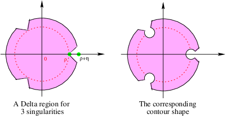
Their work is based on applying the Cauchy Integral Formula to an analytic continuation of ${\bf S}(z)$ beyond its circle of convergence. This leads to their basic notion of a Delta neighborhood $\Delta$ of $\rho$ , that is, a closed disc which is somewhat larger than the disc of radius $\rho$ , but with an open pie shaped wedge cut out at the point $z=\rho$ (see Fig. 2). We are particularly interested in their transfer theorem that directly generalizes the binomial asymptotics given in Lemma 13.

Proposition 14 ([14], Corollary 2).

Let $\rho\in(0,\infty)$ and suppose ${\bf S}$ is analytic in $\Delta\setminus\{\rho\}$ where $\Delta$ is a Delta neighborhood of $\rho$ . If $\alpha\notin{\mathbb{N}}$ and

(16)

{\bf S}(z)\ \sim\ K\big(\rho-z\big)^{\alpha}

as $z\rightarrow\rho$ in $\Delta$ , then

s(n)\ \sim[z^{n}]\,K\big(\rho-z\big)^{\alpha}\ =\ (-1)^{n}K\binom{\alpha}{n}\rho^{\alpha-n}\ \sim\ \frac{K\rho^{\alpha}}{\Gamma(-\alpha)}\cdot\rho^{-n}n^{-\alpha-1}.

Let us apply this to the square-root singularities that we are working with to see that one ends up with the asymptotics satisfying $\boldsymbol{(\star)}$ .

Corollary 15.

Suppose ${\bf S}\in{\mathbb{DOM}}[z]$ has radius of convergence $\rho\in(0,\infty)$ , and $\rho$ is the only dominant singularity of ${\bf S}$ . Furthermore suppose ${\bf A}$ and ${\bf B}$ are analytic at $0$ with ${\bf B}(0)<0$ , ${\bf A}(0)>0$ and

(17)

{\bf S}(z)\ ={\bf A}(\rho-z)+{\bf B}(\rho-z)\sqrt{\rho-z}

for $z$ in some neighborhood of $\rho$ , and $|z|<\rho$ .

Then

s(n)\ \sim\ [z^{n}]\,{\bf B}(0)\sqrt{\rho-z}\ \sim\ \frac{-{\bf B}(0)\sqrt{\rho}}{2\sqrt{\pi}}\cdot\rho^{-n}n^{-3/2}.

Proof.

One can find a Delta neighborhood $\Delta$ of $\rho$ (as in Fig. 2) such that ${\bf S}$ has an analytic continuation to $\Delta\setminus\{\rho\}$ ; and for $z\in\Delta$ and near $\rho$ one has (17) holding. Consequently

{\bf S}(z)-{\bf A}(0)\ \sim\ {\bf B}(0)\sqrt{\rho-z}

as $z\rightarrow\rho$ in $\Delta$ . This means we can apply Proposition 14 to obtain

\displaystyle s(n)

\displaystyle\sim

\displaystyle\frac{{\bf B}(0)\sqrt{\rho}}{\Gamma(-1/2)}\cdot\rho^{-n}n^{-3/2}.

∎

2.9. On the condition ${\bf B}(0)<0$

In the previous corollary suppose that ${\bf B}(0)=0$ but ${\bf B}\neq 0$ . Let $b_{k}$ be the first nonzero coefficient of ${\bf B}$ . The asymptotics for $s(n)$ are

s(n)\ \sim\ b_{k}[z^{n}]\,\big(\rho-z\big)^{k+\frac{1}{2}},

giving a law of the form $C\rho^{-n}n^{-k-\frac{3}{2}}$ . We do not know of an example of ${\bf S}$ defined by a nonlinear functional equation that gives rise to such a solution with $k>0$ , that is, with the exponent of $n$ being $-5/2$ , or $-7/2$ , etc. Meir and Moon (p. 83 of [21], 1989) give the example

w\ =\ (1/6)e^{w}\sum_{n\geq 1}z^{n}/n^{2}

where the solution $w={\bf T}$ has coefficient asymptotics given by $t_{n}\sim C/n$ .

2.10. Handling multiple dominant singularities

We want to generalize Proposition 14 to cover the case of several dominant singularities equally spaced around the circle of convergence and with the function ${\bf S}$ enjoying a certain kind of symmetry.

Proposition 16.

Given $q\in{\mathbb{P}}$ and $\rho\in(0,\infty)$ let

	$\displaystyle\omega$	$\displaystyle:=$	$\displaystyle e^{2\pi i/q}$
	$\displaystyle U_{q,\rho}$	$\displaystyle:=$	$\displaystyle\{\omega^{j}\rho:j=0,1,\ldots,q-1\}.$

Suppose $\Delta$ is a generalized Delta-neighborhood of $\rho$ with wedges removed at the points in $U_{q,\rho}$ (see Fig. 3 for $q=3$ ),

suppose ${\bf S}$ is continuous on $\Delta$ and analytic in $\Delta\setminus U_{q,\rho}$ , and suppose $d$ is a nonnegative integer such that ${\bf S}\big(\omega z\big)\ =\omega^{d}{\bf S}(z)$ for $z\in\Delta$ .

If ${\bf S}(z)\sim K(\rho-z)^{\alpha}$ as $z\rightarrow\rho$ in $\Delta$ and $\alpha\notin{\mathbb{N}}$ then

s(n)\ \sim\ \frac{qK\rho^{\alpha}}{\Gamma(-\alpha)}\cdot\rho^{-n}n^{-\alpha-1}\quad\text{if }n\equiv d\mod q,

$s(n)=0$ otherwise.

Proof.

Given $\varepsilon>0$ choose the contour ${\mathcal{C}}$ to follow the boundary of $\Delta$ except for a radius $\varepsilon$ circular detour around each singularity $\omega^{j}\rho$ (see Fig. 3). Then

s(n)\ =\ \frac{1}{2\pi i}\int_{{\mathcal{C}}}\frac{{\bf S}(z)}{z^{n+1}}dz.

Subdivide ${\mathcal{C}}$ into $q$ congruent pieces ${\mathcal{C}}_{0},\ldots,{\mathcal{C}}_{q-1}$ with ${\mathcal{C}}_{j}$ centered around $\omega^{j}\rho$ , choosing as the dividing points on ${\mathcal{C}}$ the bisecting points between successive singularities (see Fig. 4 for $q=3$ ).

Then ${\mathcal{C}}_{j}=\omega^{j}{\mathcal{C}}_{0}$ . Let $s_{j}(n)$ be the portion of the integral for $s(n)$ taken over ${\mathcal{C}}_{j}$ , that is:

s_{j}(n)\ =\ \frac{1}{2\pi i}\int_{{\mathcal{C}}_{j}}\frac{{\bf S}(z)}{z^{n+1}}dz.

Then from ${\bf S}(\omega z)=\omega^{d}{\bf S}(z)$ and ${\mathcal{C}}_{j}=\omega^{j}{\mathcal{C}}_{0}$ we have

$\displaystyle s_{j}(n)$	$\displaystyle=$	$\displaystyle\frac{1}{2\pi i}\int_{{\mathcal{C}}_{j}}\frac{{\bf S}(z)}{z^{n+1}}dz$
	$\displaystyle=$	$\displaystyle\frac{1}{2\pi i}\int_{{\mathcal{C}}_{0}}\frac{\omega^{dj}{\bf S}(z)}{(\omega^{j}z)^{n+1}}\omega^{j}dz$
	$\displaystyle=$	$\displaystyle\omega^{j(d-n)}\frac{1}{2\pi i}\int_{{\mathcal{C}}_{0}}\frac{{\bf S}(z)}{z^{n+1}}dz$
	$\displaystyle=$	$\displaystyle\omega^{j(d-n)}s_{0}(n),$

$\displaystyle s(n)$	$\displaystyle=$	$\displaystyle\sum_{j=0}^{q-1}s_{j}(n)$
	$\displaystyle=$	$\displaystyle\Big(\sum_{j=0}^{q-1}\omega^{j(d-n)}\Big)s_{0}(n)$
	$\displaystyle=$	$\displaystyle\begin{cases}qs_{0}(n)&\text{if }n\equiv d\mod q\\ 0&\text{otherwise.}\end{cases}$

We have reduced the integral calculation to the integral over ${\mathcal{C}}_{0}$ , and this proceeds exactly as in [14] in the unique singularity case described in Proposition 14. ∎

Let us apply this result to the case of ${\bf S}(z)$ having multiple dominant singularities, equally spaced on the circle of convergence, with a square-root singularity at $\rho$ .

Corollary 17.

Given $q\in{\mathbb{P}}$ and $\rho\in(0,\infty)$ let

	$\displaystyle\omega$	$\displaystyle:=$	$\displaystyle e^{2\pi i/q}$
	$\displaystyle U_{q,\rho}$	$\displaystyle:=$	$\displaystyle\{\omega^{j}\rho:j=0,1,\ldots,q-1\}.$

Suppose ${\bf S}\in{\mathbb{DOM}}[z]$ has radius of convergence $\rho\in(0,\infty)$ , $U_{q,\rho}$ is the set of dominant singularities of ${\bf S}$ , and ${\bf S}(\omega z)=\omega^{d}{\bf S}(z)$ for $|z|<\rho$ and for some $d\in{\mathbb{N}}$ .

Furthermore suppose ${\bf A}$ and ${\bf B}$ are analytic at $0$ with ${\bf B}(0)<0$ , ${\bf A}(0)>0$ and

(18)

{\bf S}(z)\ ={\bf A}(\rho-z)+{\bf B}(\rho-z)\sqrt{\rho-z}

for $z$ in some neighborhood of $\rho$ , and $|z|<\rho$ . Then

(19)

s(n)\ \sim\ \frac{q{\bf B}(0)\sqrt{\rho}}{\Gamma(-1/2)}\cdot\rho^{-n}n^{-3/2}\quad\quad\text{for }n\equiv d\mod q.

Otherwise $s(n)=0$ .

Proof.

Since the set of dominant singularities $U_{q,\rho}$ is finite one can find a generalized Delta neighborhood $\Delta$ of $\rho$ (as in Fig. 3) such that ${\bf S}$ has a continuous extension to $\Delta$ which is an analytic continuation to $\Delta\setminus U_{q,\rho}$ ; and for $z\in\Delta$ and near $\rho$ one has (18) holding. Consequently

{\bf S}(z)-{\bf A}(0)\ \sim\ {\bf B}(0)\sqrt{\rho-z}

as $z\rightarrow\rho$ in $\Delta$ . This means we can apply Proposition 16 to obtain (19). ∎

2.11. Darboux’s expansion

In 1878 Darboux [12] published a procedure for expressing the asymptotics of the coefficients $s(n)$ of a power series ${\bf S}$ with algebraic dominant singularities. Let us focus first on the case that ${\bf S}$ has a single dominant singularity, namely $z=\rho$ , and it is of square-root type, say

{\bf S}(z)\ =\ {\bf A}(\rho-z)+{\bf B}(\rho-z)\sqrt{\rho-z}

for $|z|<\rho$ and sufficiently close to $\rho$ , where ${\bf A}$ and ${\bf B}$ are analytic at 0 and ${\bf B}(0)<0$ . From Proposition 14 we know that

s(n)\ =\ \big(1+{\rm o}(1)\big)b(0)[z^{n}]\,\sqrt{\rho-z}.

Rewriting the expression for ${\bf S}(z)$ as

{\bf S}(z)\ =\ \sum_{j=0}^{\infty}\Big(a_{j}(\rho-z)^{j}\,+\,b_{j}(\rho-z)^{j+\frac{1}{2}}\Big)

we can see that the $m$ th derivative of ${\bf S}$ ‘blows up’ as $z$ approaches $\rho$ because the $m$ th derivative of the terms on the right with $j<m$ involve terms with $\rho-z$ to a negative power. However for $j\geq m$ the terms on the right have $m$ th derivatives that behave nicely near $\rho$ . By shifting the troublesome terms to the left side of the equation, giving

	$\displaystyle{\bf S}_{m}(z)$	$\displaystyle:=$	$\displaystyle{\bf S}(z)-\sum_{j<m}\Big(a_{j}(\rho-z)^{j}\,+\,b_{j}(\rho-z)^{j+\frac{1}{2}}\Big)$
		$\displaystyle=$	$\displaystyle\sum_{j\geq m}\Big(a_{j}(\rho-z)^{j}\,+\,b_{j}(\rho-z)^{j+\frac{1}{2}}\Big),$

one can see by looking at the right side that the $m$ th derivative ${\bf S}_{m}^{(m)}(z)$ of ${\bf S}_{m}(z)$ has a square-root singularity at $\rho$ provided some $b_{j}\neq 0$ for $j\geq m$ . Indeed ${\bf S}_{m}^{(m)}(z)$ is very much like ${\bf S}(z)$ , being analytic for $|z|\leq\rho$ provided $z\neq\rho$ . If $b_{m}\neq 0$ we can apply Proposition 14 to obtain (for suitable $C_{m}$ )

[z^{n}]\,{\bf S}_{m}^{(m)}(z)\ \sim\ C_{m}\rho^{-n}n^{-\frac{3}{2}}

and thus

[z^{n}]\,{\bf S}_{m}(z)\ \sim\ C_{m}\rho^{-n}n^{-m-\frac{3}{2}}.

This tells us that

s(n)\ =\ \sum_{j<m}[z^{n}]\,\Big(a_{j}(\rho-z)^{j}\,+\,b_{j}(\rho-z)^{j+\frac{1}{2}}\Big)\ +\ \big(1+{\rm o}(1)\big)C_{m}\rho^{-n}n^{-m-\frac{3}{2}}.

For $n\geq m$ the part with the $a_{j}$ drops out, so we have the Darboux expansion

s(n)\ =\ \sum_{j<m}[z^{n}]\,\Big(b_{j}(\rho-z)^{j+\frac{1}{2}}\Big)\ +\ \big(1+{\rm o}(1)\big)C_{m}\rho^{-n}n^{-m-\frac{3}{2}}.

The case of multiple dominant singularities is handled as previously. Here is the result for the general exponent $\alpha$ .

Proposition 18 (Multi Singularity Darboux Expansion).

Given $q\in{\mathbb{P}}$ let

	$\displaystyle\omega$	$\displaystyle:=$	$\displaystyle e^{2\pi i/q}$
	$\displaystyle U_{q,\rho}$	$\displaystyle:=$	$\displaystyle\{\omega^{j}\rho:j=0,1,\ldots,q-1\}.$

Suppose we have a generalized Delta-neighborhood $\Delta$ with wedges removed at the points in $U_{q,\rho}$ (see Fig. 3) and ${\bf S}$ is analytic in $\Delta\setminus U_{q,\rho}$ . Furthermore suppose $d$ is a nonnegative integer such that ${\bf S}\big(\omega z\big)\ =\omega^{d}{\bf S}(z)$ for $|z|<\rho$ .

{\bf S}(z)\ =\ {\bf A}(\rho-z)+{\bf B}(\rho-z)(\rho-z)^{\alpha}

for $|z|<\rho$ and in a neighborhood of $\rho$ , and $\alpha\notin{\mathbb{N}}$ , then given $m\in{\mathbb{N}}$ with $b_{m}\neq 0$ there is a $C_{m}\neq 0$ such that for $n\equiv d\mod q$

s(n)\ =\ q\sum_{j<m}[z^{n}]\,\Big(b_{j}(\rho-z)^{j+\frac{1}{2}}\Big)\ +\ \big(1+{\rm o}(1)\big)C_{m}\rho^{-n}n^{-\alpha-(m+1)}.

2.12. An alternative approach: reduction to the aperiodic case

In the literature one finds references to the option of using the aperiodic reduction ${\bf V}$ of ${\bf T}$ , that is, using ${\bf T}(z)=z^{d}{\bf V}(z^{q})$ where ${\bf V}(0)\neq 0$ and $\gcd\{n:v(n)\neq 0\}=1$ . ${\bf V}$ has a unique dominant singularity at $\rho_{\bf V}\,=\,{\rho_{\bf T}}^{q}$ , so the hope would be that one could use a well known result like Theorem 1 to prove that $\boldsymbol{(\star)}$ holds for $v(n)$ . Then $t(nq+d)=v(n)$ gives the asymptotics for the coefficients of ${\bf T}$ .

One can indeed make the transition from ${\bf T}={\bf E}(z,{\bf T})$ to a functional equation ${\bf V}={\bf H}(z,{\bf V})$ , but it is not clear if the property that ${\bf E}$ is holomorphic at the endpoint of the graph of ${\bf T}$ implies ${\bf H}$ is holomorphic at the endpoint of the graph of ${\bf V}$ . Instead of the property

(\exists\varepsilon>0)\,\Big({\bf E}\big(\rho+\varepsilon,{\bf T}(\rho)+\varepsilon\big)\,<\,\infty\Big)

of ${\bf E}$ used previously, a stronger version seems to be needed, namely:

(\forall y>0)\Big[{\bf E}\big(\rho,y\big)\,<\,\infty\Rightarrow\ (\exists\varepsilon>0)\,\Big({\bf E}\big(\rho+\varepsilon,y+\varepsilon\big)\,<\,\infty\Big)\Big].

We chose the singularity analysis because it sufficed to require the weaker condition that ${\bf E}$ be holomorphic at $\big(\rho,{\bf T}(\rho)\big)$ , and because the expression for the constant term in the asymptotics was far simpler that what we obtained through the use of ${\bf V}={\bf H}(z,{\bf V})$ . Furthermore, in any attempt to extend the analysis of the asymptotics to other cases of recursion of equations one would like to have the ultimate foundations of the Weierstraß Preparation Theorem and the Cauchy Integral Theorem to fall back on.

3. The Dominant Singularities of ${\bf T}(z)$

The recursion equations $w={\bf E}(z,w)$ we consider will be such that the solution $w={\bf T}$ has a radius of convergence $\rho$ in $(0,\infty)$ and finitely many dominant singularities, that is finitely many singularities on the circle of convergence. In such cases the primary technique to find the asymptotics for the coefficients $t(n)$ is to apply Cauchy’s Integral Theorem (1). Experience suggests that properly designed contours ${\mathcal{C}}$ will concentrate the value of the integral (1) on small portions of the contour near the dominant singularities of ${\bf T}$ —consequently great value is placed on locating the dominant singularities of ${\bf T}$ .

Definition 19.

For ${\bf T}\in{\mathbb{DOM}}[z]$ with radius $\rho\in(0,\infty)$ let ${\sf DomSing}({\bf T})$ be the set of dominant singularities of ${\bf T}$ , that is, the set of singularities on the circle of convergence of ${\bf T}$ .

3.1. The spectrum of a power series

Definition 20.

For ${\bf A}\in{\mathbb{DOM}}[z]$ let the spectrum ${\sf Spec}({\bf A})$ of ${\bf A}$ be the set of $n$ such that the $n$ th coefficient $a(n)$ is not zero.⁶⁶ 6 In the 1950s the logician Scholz defined the spectrum of a first-order sentence $\varphi$ to be the set of sizes of the finite models of $\varphi$ . For example if $\varphi$ is an axiom for fields, then the spectrum would be the set of powers of primes. There are many papers on this topic: a famous open problem due to Asser asks if the collection of spectra of first-order sentences is closed under complementation. This turns out to be equivalent to an open question in complexity theory. The recent paper [13] of Fischer and Makowsky has an excellent bibliography of 62 items on the subject of spectra. For our purposes, if ${\bf A}(z)$ is a generating series for a class ${\mathcal{A}}$ of combinatorial objects then the set of sizes of the objects in ${\mathcal{A}}$ is precisely ${\sf Spec}({\bf A})$ . It will be convenient to denote ${\sf Spec}({\bf A})$ simply by $A$ , so we have

A\ =\ {\sf Spec}({\bf A})\ =\ \{n:a(n)\neq 0\}.

In our analysis of the dominant singularities of ${\bf T}$ it will be most convenient to have a simple calculus to work with the spectra of power series.

3.2. An algebra of sets

The spectrum of a power series from ${\mathbb{DOM}}[z]$ is a subset of positive integers; the calculus we use has certain operations on the subsets of the nonnegative integers.

Definition 21.

For $I,J\subseteq{\mathbb{N}}$ and $j,m\in{\mathbb{N}}$ let

$\displaystyle I+J$	$\displaystyle:=$	$\displaystyle\big\{i+j:i\in I,j\in J\big\}$
$\displaystyle I-j$	$\displaystyle:=$	$\displaystyle\big\{i-j:i\in I,\big\}\quad\text{where }j\leq\min(I)$
$\displaystyle m\cdot J$	$\displaystyle:=$	$\displaystyle\{m\cdot j:j\in J\}\quad\text{for }m\geq 1$
$\displaystyle 0\odot J$	$\displaystyle:=$	$\displaystyle\{0\}$
$\displaystyle m\odot J$	$\displaystyle:=$	$\displaystyle\underbrace{J+\cdots+J}_{m-{\rm times}}\quad\text{for $m\geq 1$}$
$\displaystyle I\odot J$	$\displaystyle:=$	$\displaystyle\bigcup_{i\in I}i\odot J$
$\displaystyle m\|J$	$\displaystyle\Leftrightarrow$	$\displaystyle\big(\forall j\in J\big)\,(m\|j).$

3.3. The periodicity constants

Periodicity plays an important role in determining the dominant singularities. For example the generating series ${\bf T}(z)$ of planar (0,2)-binary trees, that is, planar trees where each node has 0 or 2 successors, is defined by

{\bf T}(z)\ =\ z+z{\bf T}(z)^{2}.

It is clear that all such trees have odd size, so one has

{\bf T}(z)\ =\ \sum_{j=0}^{\infty}t(2j+1)z^{2j+1}\ =\ z\sum_{j=0}^{\infty}t(2j+1)(z^{2})^{j}.

This says we can write ${\bf T}(z)$ in the form

{\bf T}(z)\ =\ z{\bf V}(z^{2}).

From such considerations one finds that ${\bf T}(z)$ has exactly two dominant singularities, $\rho$ and $-\rho$ . (The general result is given in Lemma 26.)

Lemma 22.

For ${\bf A}\in{\mathbb{DOM}}[z]$ let

p\ :=\ \gcd A\qquad d\ :=\ \min A\qquad q\ :=\ \gcd(A-d).

Then there are ${\bf U}(z)$ and ${\bf V}(z)$ in ${\mathbb{R}}^{\geq 0}[[z]]$ such that

a

${\bf A}(z)\ =\ {\bf U}\big(z^{p}\big)$ with $\gcd(U)=1$
b

${\bf A}(z)=z^{d}{\bf V}\big(z^{q}\big)$ with ${\bf V}(0)\neq 0$ and $\gcd(V)=1$ .

Proof.

(Straightforward.) ∎

Definition 23.

With the notation of Lemma 22, ${\bf U}(z^{p})$ is the purely periodic form of ${\bf A}(z)$ ; and $z^{d}{\bf V}\big(z^{q}\big)$ is the shift periodic form of ${\bf A}(z)$ .

The next lemma is quite important—it says that the $q$ equally spaced points on the circle of convergence are all dominant singularities of ${\bf T}$ . Our main results depend heavily on the fact that the equations we consider are such that these are the only dominant singularities of ${\bf T}$ .

Lemma 24.

Let ${\bf T}\in{\mathbb{DOM}}[z]$ have radius of convergence $\rho\in(0,\infty)$ and the shift periodic form $z^{d}{\bf V}(z^{q})$ . Then

\{z:z^{q}=\rho^{q}\}\ \subseteq\ {\sf DomSing}({\bf T}).

Proof.

Suppose ${z_{0}}^{q}=\rho^{q}$ and suppose ${\bf S}(z)$ is an analytic continuation of ${\bf T}(z)$ into a neighborhood ${\mathbb{D}}_{\varepsilon}(z_{0})$ of $z_{0}$ . Let $\omega:=z_{0}/\rho$ . Then $\omega^{q}=1$ . The function ${\bf S}_{0}(z):={\bf S}(\omega z)/\omega^{d}$ is an analytic function on ${\mathbb{D}}_{\varepsilon}(\rho)$ . For $z\in{\mathbb{D}}_{\varepsilon}(\rho)\cap{\mathbb{D}}_{\rho}(0)$ we have

\omega z\in{\mathbb{D}}_{\varepsilon}(z_{0})\cap{\mathbb{D}}_{\rho}(0),

{\bf S}_{0}(z)\ =\ {\bf S}(\omega z)/\omega^{d}\ =\ {\bf T}(\omega z)/\omega^{d}\ =\ {\bf T}(z).

This means ${\bf S}_{0}(z)$ is an analytic continuation of ${\bf T}(z)$ at $z=\rho$ , contradicting Pringsheim’s Theorem that $\rho$ is a dominant singularity. ∎

3.4. Determining the shift periodic parameters from ${\bf E}$

Lemma 25.

Suppose ${\bf T}(z)={\bf E}\big(z,{\bf T}(z)\big)$ is a formal recursion that defines ${\bf T}\in{\mathbb{DOM}}[z]$ , where ${\bf E}\in{\mathbb{DOM}}[z,w]$ . Let the shift periodic form of ${\bf T}(z)$ be $z^{d}{\bf V}(z^{q})$ . Then

	$\displaystyle d$	$\displaystyle=$	$\displaystyle\min(T)\ =\ \min(E_{0})$
	$\displaystyle q$	$\displaystyle=$	$\displaystyle\gcd(T-d)\ =\ \gcd\bigcup_{n\geq 0}\Big(E_{n}+(n-1)d\Big).$

Proof.

Since ${\bf T}$ is recursively defined by

{\bf T}(z)\ =\ \sum_{n\geq 0}{\bf E}_{n}(z){\bf T}(z)^{n}

one has the first nonzero coefficient of ${\bf T}$ being the first nonzero coefficient of ${\bf E}_{0}$ , and thus $d=\min(T)=\min(E_{0})$ . It is easy to see that we also have $q=\gcd(T-d)$ .

Next apply the spectrum operator to the above functional equation to obtain the set equation

T\ =\ \bigcup_{n\geq 0}E_{n}+n\odot T,

and thus

T-d\ =\ \bigcup_{n\geq 0}\Big(E_{n}+(n-1)d+n\odot(T-d)\Big).

Since $q=\gcd(T-d)$ it follows that $q|r:=\gcd\Big(\bigcup_{n}E_{n}+(n-1)d\Big)$ .

To show that $r|q$ , and hence that $r=q$ , note that

w=\ \bigcup_{n\geq 0}\Big(E_{n}+(n-1)d+n\odot w\Big)

is a recursion equation whose unique solution is $w=T-d$ . Furthermore we can find the solution $w$ by iteratively applying the set operator

\Theta(w)\ :=\ \bigcup_{n\geq 0}\Big(E_{n}+(n-1)d+n\odot w\Big)

to Ø, that is,

T-d\ =\ \lim_{n\rightarrow\infty}\Theta^{n}(\text{\O}).

Clearly $r\,|\,\text{\O}$ , and a simple induction shows that for every $n$ we have $r\,\big|\,\Theta^{n}(\text{\O})$ . Thus $r\,|\,(T-d)$ , so $r\,|\,q$ , giving $r=q$ . This finishes the proof that $q$ is the gcd of the set $\bigcup_{n}\Big(E_{n}+(n-1)d\Big)$ . ∎

3.5. Determination of the dominant singularities

The following lemma completely determines the dominant singularities of ${\bf T}$ .

Lemma 26.

Suppose

a

${\bf T}\in{\mathbb{DOM}}[z]$ has radius of convergence $\rho\in(0,\infty)$ with ${\bf T}(\rho)<\infty$ , and
b

${\bf T}(z)={\bf E}\big(z,{\bf T}(z)\big)$ , where ${\bf E}\in{\mathbb{DOM}}[z,w]$ is nonlinear in $w$ and holomorphic on (the graph of) ${\bf T}$ .

Let the shift periodic form of ${\bf T}(z)$ be $z^{d}{\bf V}(z^{q})$ . Then

{\sf DomSing}({\bf T})\ =\ \{z:z^{q}=\rho^{q}\}.

Proof.

By the usual application of the implicit function theorem, if $z$ is a dominant singularity of ${\bf T}$ then

(20)

{\bf E}_{w}\big(z,{\bf T}(z)\big)=1.

As $\rho$ is a dominant singularity we can replace (20) by

(21)

{\bf E}_{w}\big(z,{\bf T}(z)\big)\ =\ {\bf E}_{w}\big(\rho,{\bf T}(\rho)\big).

Let ${\bf U}(z^{p})$ be the purely periodic form of ${\bf E}_{w}\big(z,{\bf T}(z)\big)$ . As the coefficients of ${\bf E}_{w}$ are nonnegative it follows that (21) implies

{\sf DomSing}({\bf T})\ \subseteq\ \{z:z^{p}=\rho^{p}\}.

We know from Lemma 24 that

\{z:z^{q}=\rho^{q}\}\ \subseteq\ {\sf DomSing}({\bf T}),

consequently $q|p$ .

To show that $p\leq q$ first note that if $m\in{\mathbb{N}}$ then

\gcd(m+T)\,\big|\,q.

Since

{\bf U}(z^{p})\ =\ {\bf E}_{w}\big(z,{\bf T}(z)\big)\ =\ \sum_{n\geq 1}{\bf E}_{n}(z)n{\bf T}(z)^{n-1},

applying the spectrum operator gives

\displaystyle{\sf Spec}\big({\bf U}(z^{p})\big)

\displaystyle=

\displaystyle\bigcup_{n\geq 1}E_{n}+(n-1)\odot T.

Choose $n\geq 2$ such that $E_{n}\neq\text{\O}$ and choose $a\in E_{n}$ . Then

	$\displaystyle{\sf Spec}\big({\bf U}(z^{p})\big)$	$\displaystyle\supseteq$	$\displaystyle E_{n}+(n-1)\odot T$
		$\displaystyle\supseteq$	$\displaystyle\big(a+(n-2)d\big)+T,$

so taking the $\gcd$ of both sides gives

	$\displaystyle p$	$\displaystyle=$	$\displaystyle\gcd{\sf Spec}\big({\bf U}(z^{p})\big)$
		$\displaystyle\leq$	$\displaystyle\gcd\Big(\big(a+(n-2)d\big)+T\Big)\,\Big\|\,q.$

With $p=q$ it follows that we have proved the dominant singularities are as claimed. ∎

3.6. Solutions that converge at the radius of convergence

The equations $w=\Theta(w)$ that we are pursuing will have a solution ${\bf T}$ that converges at the finite and positive radius of convergence $\rho_{\bf T}$ .

Definition 27.

Let

{\mathbb{DOM}}^{\star}[z]\ :=\ \{{\bf T}\in{\mathbb{DOM}}[z]:\rho_{\bf T}\in(0,\infty),\ {\bf T}(\rho_{\bf T})<\infty\}.

3.7. A basic theorem

The next theorem summarizes what we need from the preceding discussions to show that ${\bf T}={\bf E}(z,{\bf T})$ leads to $\boldsymbol{(\star)}$ holding for the coefficients $t_{n}$ of ${\bf T}$ .

Theorem 28.

Suppose ${\bf T}\in{\mathbb{DOM}}[z]$ and ${\bf E}\in{\mathbb{DOM}}[z,w]$ are such that

a

${\bf T}(z)={\bf E}\big(z,{\bf T}(z)\big)$ holds as an identity between formal power series
b

${\bf T}\in{\mathbb{DOM}}^{\star}[z]$
c

${\bf E}(z,w)$ is nonlinear in $w$
d

${\bf E}_{z}\neq 0$
e

$(\exists\varepsilon>0)\,\Big({\bf E}\big(\rho+\varepsilon,{\bf T}(\rho)+\varepsilon\big)\,<\,\infty\Big)$ .

Then

t(n)\ \sim\ q\sqrt{\frac{\rho{\bf E}_{z}\big(\rho,{\bf T}(\rho)\big)}{2\pi{\bf E}_{ww}\big(\rho,{\bf T}(\rho)\big)}}\rho^{-n}n^{-3/2}\quad\text{for }n\equiv d\mod q.

Otherwise $t(n)=0$ . Thus $\boldsymbol{(\star)}$ holds on $\{n:t(n)>0\}$ .

Proof.

By Corollary 12, Corollary 17 and Lemma 26. ∎

4. Recursion Equations using Operators

Throughout the theoretical section, $\lx@sectionsign\,$ 2, we only considered recursive equations based on elementary operators ${\bf E}(z,w)$ . Now we want to expand beyond these to include recursions that are based on popular combinatorial constructions used with classes of unlabelled structures. As an umbrella concept to create these various recursions we introduce the notion of operators $\Theta$ .

Actually if one is only interested in working with classes of labelled structures then it seems that the recursive equations based on elementary power series are all that one needs. However, when working with classes of unlabelled structures, the natural way of writing down an equation corresponding to a recursive specification is in terms of combinatorial operators like ${\sf MSet}$ and ${\sf Seq}$ . The resulting equation $w=\Theta(w)$ , if properly designed, will have a unique solution ${\bf T}(z)$ whose coefficients are recursively defined, and this solution will likely be needed to construct the translation of $w=\Theta(w)$ to an elementary recursion $w={\bf E}(z,w)$ , a translation that is needed in order to apply the theoretical machinery of $\lx@sectionsign\,$ 2.

4.1. Operators

The mappings on generating series corresponding to combinatorial constructions are called operators. But we want to go beyond the obvious and include complex combinations of elementary and combinatorial operators. For this purpose we introduce a very general definition of an operator.

Definition 29.

An operator is a mapping $\Theta:{\mathbb{DOM}}[z]\,\rightarrow\,{\mathbb{DOM}}[z]$ .

Note that operators $\Theta$ act on ${\mathbb{DOM}}[z]$ , the set of formal power series with nonnegative coefficients and constant term 0. As mentioned before, the constraint that the constant terms of the power series be 0 makes for an elegant theory because compositions of operators are always defined.

A primary concern, as in the original work of Pólya, is to be able to handle combinatorial operators $\Theta$ that, when acting on ${\bf T}(z)$ , introduce terms like ${\bf T}(z^{2}),{\bf T}(z^{3})$ etc. For such operators it is natural to use power series ${\bf T}(z)$ with integer coefficients as one is usually working in the context of ordinary generating functions. In such cases one has $\rho\leq 1$ for the radius of convergence of ${\bf T}$ , provided ${\bf T}$ is not a polynomial.

Definition 30.

An integral operator is a mapping $\Theta:{\mathbb{IDOM}}[z]\,\rightarrow\,{\mathbb{IDOM}}[z]$ , where ${\mathbb{IDOM}}[z]\ :=\ \big\{{\bf A}\in{\mathbb{N}}[[z]]:{\bf A}(0)=0\big\}$ , the set of power series with nonnegative integer coefficients and constant term zero.

Remark 31.

Many of the lemmas, etc, that follow have both a version for general operators and a version for integral operators. We will usually just state and prove the general version, leaving the completely parallel integral version as a routine exercise.

4.2. The arithmetical operations on operators

The operations of addition, multiplication, positive scalar multiplication and composition are defined on the set of operators in the natural manner:

Definition 32.

$\displaystyle(\Theta_{1}\,+\,\Theta_{2})({\bf T})$	$\displaystyle:=$	$\displaystyle\Theta_{1}({\bf T})\,+\,\Theta_{2}({\bf T})$
$\displaystyle(\Theta_{1}\,\cdot\,\Theta_{2})({\bf T})$	$\displaystyle:=$	$\displaystyle\Theta_{1}({\bf T})\,\cdot\,\Theta_{2}({\bf T})$
$\displaystyle(c\cdot\Theta)({\bf T})$	$\displaystyle:=$	$\displaystyle c\cdot\Theta({\bf T})$
$\displaystyle(\Theta_{1}\,\circ\,\Theta_{2})({\bf T})$	$\displaystyle:=$	$\displaystyle\Theta_{1}\big(\Theta_{2}({\bf T})\big)\,,$

where the operations on the right side are the operations of formal power series. A set of operators is closed if it is closed under the four arithmetical operations.

Note that when working with integral operators the scalars should be positive integers. The operation of addition corresponds to the construction disjoint union and the operation of product to the construction disjoint sum, for both the unlabelled and the labelled case. Clearly the set of all [integral] operators is closed.

4.3. Elementary operators

In a most natural way we can think of elementary power series ${\bf E}(z,w)$ as operators.

Definition 33.

Given ${\bf E}(z,w)\in{\mathbb{DOM}}[z,w]$ let the associated elementary operator be given by

{\bf E}:{\bf T}\mapsto{\bf E}(z,{\bf T})\quad\text{for }{\bf T}\in{\mathbb{DOM}}.

Two particular kinds of elementary operators are as follows.

Definition 34.

Let ${\bf A}\in{\mathbb{DOM}}[z]$ .

a

The constant operator $\Theta_{\bf A}$ is given by $\Theta_{\bf A}:{\bf T}\mapsto{\bf A}$ for ${\bf T}\in{\mathbb{DOM}}[z]$ , and
b

the simple operator ${\bf A}(w)$ maps ${\bf T}\in{\mathbb{DOM}}[z]$ to the power series that is the formal expansion of

$\sum_{n\geq 1}a_{n}\Big(\sum_{j\geq 1}t_{j}z^{j}\Big)^{n}\,.$

4.4. Open elementary operators

Definition 35.

Given $a,b>0$ , an elementary operator ${\bf E}(z,w)$ is open at $(a,b)$ if

(\exists\varepsilon>0)\Big({\bf E}(a+\varepsilon,b+\varepsilon)<\infty\Big).

${\bf E}$ is open if it is open at any $a,b>0$ for which ${\bf E}(a,b)<\infty$ .

Eventually we will be wanting an elementary operator to be open at $\big(\rho,{\bf T}(\rho)\big)$ in order to invoke the Weierstraß Preparation Theorem.

Lemma 36.

Suppose ${\bf A}\in{\mathbb{DOM}}[z]$ and $a,b>0$ .
The constant operator $\Theta_{\bf A}$

a

is open at $(a,b)$ iff $a<\rho_{\bf A}$ ;
b

it is open iff $\rho_{\bf A}>0\ \Rightarrow\ {\bf A}(\rho_{\bf A})=\infty$ .

The simple operator $\Theta_{\bf A}$

(c)

is open at $(a,b)$ iff $b<\rho_{\bf A}$ ;
(d)

it is open iff $\rho_{\bf A}>0\ \Rightarrow\ {\bf A}(\rho_{\bf A})=\infty$ .

Proof.

$\Theta_{\bf A}$ is open at $(a,b)$ iff for some $\varepsilon>0$ we have ${\bf A}(a+\varepsilon)<\infty$ . This is clearly equivalent to $a<\rho_{\bf A}$ .

Thus $\rho_{\bf A}>0$ and ${\bf A}(\rho_{\bf A})<\infty$ imply $\Theta_{\bf A}$ is not open at $(\rho_{\bf A},b)$ for any $b>0$ , hence it is not open. Conversely if $\Theta_{\bf A}$ is not open then $\rho_{\bf A}>0$ and ${\bf A}(a)<\infty$ for some $a,b>0$ , but ${\bf A}(a+\varepsilon)=\infty$ for any $\varepsilon>0$ . This implies $a=\rho_{\bf A}$ .

The proof for the simple operator ${\bf A}(w)$ is similar. ∎

4.5. Operational closure of the set of open ${\bf E}$

Lemma 37.

Let $a,b>0$ .

a

The set of elementary operators open at $(a,b)$ is closed under the arithmetical operations of scalar multiplication, addition and multiplication. If ${\bf E}_{2}$ is open at $(a,b)$ and ${\bf E}_{1}$ is open at $\big(a,{\bf E}_{2}(a,b)\big)$ then ${\bf E}_{1}\big(z,{\bf E}_{2}(z,w)\big)$ is open at $(a,b)$ .
b

The set of open elementary operators is closed.

Proof.

Let $c>0$ and let ${\bf E},{\bf E}_{1},{\bf E}_{2}$ be elementary operators open at $(a,b)$ . Then

$\displaystyle(\exists\varepsilon>0)\,{\bf E}\big(a+\varepsilon,b+\varepsilon\big)<\infty$	$\displaystyle\Rightarrow$	$\displaystyle(\exists\varepsilon>0)\,(c{\bf E})\big(a+\varepsilon,b+\varepsilon\big)<\infty$
$\displaystyle(\exists\varepsilon_{1}>0)\,{\bf E}_{1}\big(a+\varepsilon_{1},b+\varepsilon_{1}\big)<\infty$	and	$\displaystyle(\exists\varepsilon_{2}>0)\,{\bf E}_{2}\big(a+\varepsilon_{2},b+\varepsilon_{2}\big)<\infty$
	$\displaystyle\Rightarrow$	$\displaystyle(\exists\varepsilon>0){\bf E}_{i}\big(a+\varepsilon,b+\varepsilon\big)<\infty\ \text{for}\ i=1,2$
	$\displaystyle\Rightarrow$	$\displaystyle(\exists\varepsilon>0)\,\big({\bf E}_{1}+{\bf E}_{2}\big)(a+\varepsilon,b+\varepsilon)<\infty$
$\displaystyle(\exists\varepsilon_{1}>0)\,{\bf E}_{1}\big(a+\varepsilon_{1},b+\varepsilon_{1}\big)<\infty$	and	$\displaystyle(\exists\varepsilon_{2}>0)\,{\bf E}_{2}\big(a+\varepsilon_{2},b+\varepsilon_{2}\big)<\infty$
	$\displaystyle\Rightarrow$	$\displaystyle(\exists\varepsilon>0){\bf E}_{i}\big(a+\varepsilon,b+\varepsilon\big)<\infty\ \text{for}\ i=1,2$
	$\displaystyle\Rightarrow$	$\displaystyle(\exists\varepsilon>0)\,\big({\bf E}_{1}{\bf E}_{2}\big)(a+\varepsilon,b+\varepsilon)<\infty.$

Now suppose ${\bf E}_{2}$ is open at $(a,b)$ and ${\bf E}_{1}$ is open at $\big(a,{\bf E}_{1}(a,b)\big)$ . Then

	$\displaystyle(\exists\varepsilon_{2}>0)\,{\bf E}_{2}\big(a+\varepsilon_{2},b+\varepsilon_{2}\big)<\infty$	and	$\displaystyle(\exists\varepsilon_{1}>0)\,{\bf E}_{1}\big(a+\varepsilon_{1},{\bf E}_{2}(a,b)+\varepsilon_{1}\big)<\infty$
		$\displaystyle\Rightarrow$	$\displaystyle(\exists\varepsilon>0)\,{\bf E}_{1}\big(a+\varepsilon,{\bf E}_{2}(a+\varepsilon,b+\varepsilon)+\varepsilon\big)<\infty.$

This completes the proof for (a). Part (b) is proved similarly. ∎

The base operators that we will use as a starting point are the elementary operators ${\bf E}$ and all possible restrictions $\Theta_{\mathbb{M}}$ of the standard operators $\Theta$ of combinatorics discussed below. More complex operators called composite operators will be fabricated from these base operators by using the familiar arithmetical operations of addition, multiplication, scalar multiplication and composition discussed in $\lx@sectionsign\,$ 4.2.

4.6. The standard operators on ${\mathbb{DOM}}[z]$

Following the lead of Flajolet and Sedgewick [15] we adopt as our standard operators ${\sf MSet}$ (multiset), ${\sf Cycle}$ (undirected cycle), ${\sf DCycle}$ (directed cycle) and ${\sf Seq}$ (sequence), corresponding to the constructions by the same names.⁷⁷ 7 Flajolet and Sedgewick also include ${\sf Set}$ as a standard operator, but we will not do so since, as mentioned in the second paragraph of $\lx@sectionsign$ 2, for a given ${\bf T}$ , the series ${\bf G}(z,w)$ associated with ${\sf Set}({\bf T})$ may very well not be elementary. For a discussion of mixed sign equations see $\lx@sectionsign\,$ 6. These operators have well known analytic expressions, for example,

\begin{array}[]{l l}\text{unlabelled multiset operator}&1+{\sf MSet}({\bf T})\ =\ \exp\Big(\sum_{j\geq 1}{\bf T}(z^{j})/j\Big)\\ \text{labelled multiset operator}&\widehat{\sf MSet}({\bf T})\ =\ \sum_{j\geq 1}{\bf T}(z)^{j}/j!\ =\ e^{{\bf T}(z)}-1\end{array}

4.7. Restrictions of standard operators

Let ${\mathbb{M}}\subseteq{\mathbb{P}}$ . (We will always assume ${\mathbb{M}}$ is nonempty.) The ${\mathbb{M}}$ -restriction of a standard construction $\Delta$ applied to a class of trees means that one only takes those forests in $\Delta({\mathcal{T}})$ where the number of trees is in ${\mathbb{M}}$ . Thus ${\sf MSet}_{\{2,3\}}({\mathcal{T}})$ takes all multisets of two or three trees from ${\mathcal{T}}$ .

The Pólya cycle index polynomials ${\bf Z}({\sf H},z_{1},\ldots,z_{m})$ are very convenient for expressing such operators; such a polynomial is connected with a permutation group ${\sf H}$ acting on an $m$ -element set (see Harary and Palmer [16], p. 35). For $\sigma\in{\sf H}$ let $\sigma_{j}$ be the number of $j$ -cycles in a decomposition of $\sigma$ into disjoint cycles. Then

{\bf Z}({\sf H},z_{1},\ldots,z_{m})\ :=\ \frac{1}{|H|}\sum_{\sigma\in H}\prod_{j=1}^{m}{z_{j}}^{\sigma_{j}}.

The only groups we consider are the following:

a

${\sf S}_{m}$ is the symmetric group on $m$ elements,
b

${\sf D}_{m}$ the dihedral group of order $2m$ ,
c

${\sf C}_{m}$ the cyclic group of order $m$ , and
d

${\sf Id}_{m}$ the one-element identity group on $m$ elements.

The ${\mathbb{M}}$ -restrictions of the standard operators are each of the form $\Delta_{\mathbb{M}}\,:=\,\sum_{m\in{\mathbb{M}}}\Delta_{m}$ where $\Delta\in\{{\sf MSet},{\sf DCycle},{\sf Cycle},{\sf Seq}\}$ and $\Delta_{m}$ is given by:

\begin{array}[]{l l| l l}{\sf operator}&{\sf unlabelled\ case}&{\sf operator}&{\sf labelled\ case}\\ {\sf MSet}_{m}({\bf T})&{\bf Z}\big({\sf S}_{m},{\bf T}(z),\ldots,{\bf T}(z^{m})\big)&\widehat{\sf MSet}_{m}({\bf T})&(1/m!){\bf T}(z)^{m}\\ {\sf Cycle}_{m}({\bf T})&{\bf Z}\big({\sf D}_{m},{\bf T}(z),\ldots,{\bf T}(z^{m})\big)&\widehat{\sf Cycle}_{m}({\bf T})&(1/2m){\bf T}(z)^{m}\\ {\sf DCycle}_{m}({\bf T})&{\bf Z}\big({\sf C}_{m},{\bf T}(z),\ldots,{\bf T}(z^{m})\big)&\widehat{\sf DCycle}_{m}({\bf T})&(1/m){\bf T}(z)^{m}\\ {\sf Seq}_{m}({\bf T})&{\bf Z}\big({\sf Id}_{m},{\bf T}(z),\ldots,{\bf T}(z^{m})\big)&\widehat{\sf Seq}_{m}({\bf T})&{\bf T}(z)^{m}\\ \end{array}

Note that the labelled version of $\Delta_{m}$ is just the first term of the cycle index polynomial for the unlabelled version, and the sequence operators are the same in both cases. We write simply ${\sf MSet}$ for ${\sf MSet}_{\mathbb{M}}$ if ${\mathbb{M}}$ is ${\mathbb{P}}$ , etc.

In the labelled case the standard operators (with restrictions) are simple operators, whereas in the unlabelled case only $\Delta_{\{1\}}$ and the ${\sf Seq}_{\mathbb{M}}$ are simple. The other standard operators in the unlabelled case are not elementary because of the presence of terms ${\bf T}(z^{j})$ with $j>1$ when ${\mathbb{M}}\neq\{1\}$ .

4.8. Examples of recursion equations

Table 1 gives the recursion equations for the generating series of several well-known classes of trees.

\begin{array}[]{l @{\quad} l}\text{Recursion Equation}\hfil\hskip 9.24994pt&\text{Class of Rooted Trees}\\ \hline\cr w\,=\,z\,+\,zw\hfil\hskip 9.24994pt&\text{chains}\\ w\,=\,z\,+\,z{\sf Seq}(w)\hfil\hskip 9.24994pt&\text{planar}\\ w\,=\,mz\,+\,mz{\sf Seq}(w)\hfil\hskip 9.24994pt&\text{$m$-flagged planar}\\ w\,=\,ze^{w}\hfil\hskip 9.24994pt&\text{labelled}\\ w\,=\,z\,+\,z{\sf MSet}(w)\hfil\hskip 9.24994pt&\text{unlabelled }\\ w\,=\,z\,+\,z{\sf MSet}_{\{2,3\}}(w)\hfil\hskip 9.24994pt&\text{unlabelled (0,2,3)-}\\ w\,=\,z\,+\,z{\sf Seq}_{2}(w)\hfil\hskip 9.24994pt&\text{unlabelled binary planar}\\ w\,=\,z\,+\,z{\sf MSet}_{2}(w)\hfil\hskip 9.24994pt&\text{unlabelled binary }\\ w\,=\,z\,+\,zw^{2}\hfil\hskip 9.24994pt&\text{labelled binary }\\ w\,=\,z\,+\,z\big(w\,+\,{\sf MSet}_{2}(w)\big)\hfil\hskip 9.24994pt&\text{unlabelled unary-binary }\\ w\,=\,z\,+\,z{\sf MSet}_{r}(w)\hfil\hskip 9.24994pt&\text{unlabelled $r$-regular }\\ \hline\cr\end{array}

Table 1. Familiar examples of recursion equations

4.9. Key properties of operators

Now we give a listing of the various properties of abstract operators that are needed to prove a universal law for recursion equations. The first question to be addressed is “Which properties does $\Theta$ need in order to guarantee that $w=\Theta(w)$ has a solution?”

4.10. Retro operators

There is a simple natural property of an operator $\Theta$ that guarantees an equation $w=\Theta(w)$ has a unique solution that is determined by a recursive computation of the coefficients, namely $\Theta$ calculates, given ${\bf T}$ , the $n$ th coefficient of $\Theta({\bf T})$ solely on the basis of the values of $t(1),\ldots,t(n-1)$ .

Definition 38.

An operator $\Theta$ is retro if there is a sequence $\sigma$ of functions such that for ${\bf B}\,=\,\Theta({\bf A})$ one has $b_{n}\,=\,\sigma_{n}(a_{1},\ldots,a_{n-1})$ , where $\sigma_{1}$ is a constant .

There is a strong temptation to call such $\Theta$ recursion operators since they will be used to recursively define generating series. But without the context of a recursion equation there is nothing recursive about $b_{n}$ being a function of $a_{1},\ldots,a_{n-1}$ .

Lemma 39.

A retro operator $\Theta$ has a unique fixpoint in ${\mathbb{DOM}}[z]$ , that is, there is a unique power series ${\bf T}\,\in\,{\mathbb{DOM}}[z]$ such that ${\bf T}\,=\,\Theta({\bf T})\,.$ We can obtain ${\bf T}$ by an iterative application of $\Theta$ to the constant power series $0$ :

{\bf T}\ =\ \lim_{n\rightarrow\infty}\Theta^{n}(0)\,.

If $\Theta$ is an integral retro operator then ${\bf T}\in{\mathbb{IDOM}}[z]$ .

Proof.

Let $\sigma$ be the sequence of functions that witness the fact that $\Theta$ is retro. If ${\bf T}=\Theta({\bf T})$ then

	$\displaystyle t(1)$	$\displaystyle=$	$\displaystyle\sigma_{1}$
	$\displaystyle t(n)$	$\displaystyle=$	$\displaystyle\sigma_{n}\big(t(1),\ldots,t(n-1)\big)\quad\text{for }n>1.$

Thus there is at most one possible fixpoint ${\bf T}$ of $\Theta$ ; and these two equations show how to recursively find such a ${\bf T}$ .

A simple argument shows that $\Theta^{n+k}(0)$ agrees with $\Theta^{n}(0)$ on the first $n$ coefficients, for all $k\geq 0$ . Thus $\lim_{n\rightarrow\infty}\Theta^{n}(0)$ is a fixpoint, and hence the fixpoint . If $\Theta$ is also integral then each stage $\Theta^{n}(0)\in{\mathbb{IDOM}}[z]$ , so ${\bf T}\in{\mathbb{IDOM}}[z]$ . ∎

Thus if $\Theta$ is a retro operator then the functional equation $w=\Theta(w)$ has a unique solution ${\bf T}(z)$ . Although the end goal is to have an equation $w=\Theta(w)$ with $\Theta$ a retro operator, for the intermediate stages it is often more desirable to work with weakly retro operators.

Definition 40.

An operator $\Theta$ is weakly retro if there is a sequence $\sigma$ of functions such that for ${\bf B}\,=\,\Theta({\bf A})$ one has $b_{n}\,=\,\sigma_{n}(a_{1},\ldots,a_{n})$ .

Lemma 41.

a

The set of retro operators is closed.
b

The set of weakly retro operators is closed and includes all elementary operators and all restrictions of standard operators.
c

If $\Theta$ is a weakly retro operator then $z\Theta$ and $w\Theta$ are both retro operators.

Proof.

For (a), given retro operators $\Theta,\Theta_{1},\Theta_{2}$ , a positive constant $c$ and a power series ${\bf T}\unrhd 0$ , we have

$\displaystyle{[z^{n}]\,}(c\Theta)({\bf T})$	$\displaystyle=$	$\displaystyle c\big([z^{n}]\,\Theta({\bf T})\big)$
$\displaystyle{[z^{n}]\,}(\Theta_{1}+\Theta_{2})({\bf T})$	$\displaystyle=$	$\displaystyle[z^{n}]\,\Theta_{1}({\bf T})+[z^{n}]\,\Theta_{2}({\bf T})$
$\displaystyle{[z^{n}]\,}(\Theta_{1}\Theta_{2})({\bf T})$	$\displaystyle=$	$\displaystyle\sum_{j=1}^{n-1}[z^{j}]\,\Theta_{1}({\bf T})[z^{n-j}]\Theta_{2}({\bf T})$
$\displaystyle{[z^{n}]\,}(\Theta_{1}\circ\Theta_{2})({\bf T})$	$\displaystyle=$	$\displaystyle\sigma_{n}\big([z^{1}]\Theta_{2}({\bf T}),\ldots,[z^{n}]\,\Theta_{2}({\bf T})\big),$

where $\sigma$ is the sequence of functions that witness the fact that $\Theta_{1}$ is a retro operator. In each case it is clear that the value of the right side depends only on the first $n-1$ coefficients of ${\bf T}$ . Thus the set of retro operators is closed.

For (b) use the same proof as in (a), after changing the initial operators to weakly retro operators, to show that the set of weakly retro operators is closed.

For an elementary operator ${\bf E}(z,w)$ and power series ${\bf T}\unrhd 0$ we have, after writing ${\bf E}(z,w)$ as $\sum_{i\geq 0}{\bf E}_{i}(z)w^{i}$ ,

	$\displaystyle{[z^{n}]\,}{\bf E}\big(z,{\bf T}(z)\big)$	$\displaystyle=$	$\displaystyle[z^{n}]\,\sum_{j\geq 0}{\bf E}_{j}(z){\bf T}(z)^{j}$
		$\displaystyle=$	$\displaystyle\sum_{j\geq 0}\sum_{i=0}^{n}e_{ij}\big[z^{n-i}\big]{\bf T}(z)^{j}.$

The last expression clearly depends only on the first $n$ coefficients of ${\bf T}(z)$ . Thus all elementary operators are weakly retro operators.

Let $Z({\bf H},z_{1},\ldots,z_{m})$ be a cycle index polynomial. Then for ${\bf T}\in{\mathbb{DOM}}[z]$ one has

{[z^{n}}]{\bf T}(z^{j})\ =\ \begin{cases}0&\text{if $j$ does not divide $n$}\\ t(n/j)&\text{if }j|n.\end{cases}

Thus the operator that maps ${\bf T}(z)$ to ${\bf T}(z^{j})$ is a weakly retro operator. The set of weakly retro operators is closed, so the operator mapping ${\bf T}$ to $Z\big({\bf H},{\bf T}(z),\ldots,{\bf T}(z^{m})\big)$ is weakly retro. Now every restriction $\Delta_{\mathbb{M}}$ of a standard operator is a (possibly infinite) sum of such instances of cycle index polynomials; thus they are also weakly retro.

For (c) note that

	$\displaystyle{[z^{n}]}\,\big(z\Theta({\bf T})\big)$	$\displaystyle=$	$\displaystyle[z^{n-1}]\,\Theta({\bf T})$
	$\displaystyle{[z^{n}]}\,\big({\bf T}\Theta({\bf T})\big)$	$\displaystyle=$	$\displaystyle\sum_{j=1}^{n-1}t_{j}[z^{n-j}]\,\Theta({\bf T}),$

and in both cases the right side depends only on $t_{1},\ldots,t_{n-1}$ .

∎

Lemma 42.

a

An elementary operator ${\bf E}(z,w)=\sum_{ij}e_{ij}z^{i}w^{j}$ is retro iff $e_{01}=0$ .
b

A restriction $\Delta_{\mathbb{M}}$ of a standard operator $\Delta$ is retro iff $1\notin{\mathbb{M}}$ .

Proof.

For (a) let ${\bf T}\in{\mathbb{DOM}}[z]$ . Then

[z^{n}]\,{\bf E}\big(z,{\bf T}(z)\big)\ =\ \sum_{j\geq 0}\sum_{i=0}^{n}e_{ij}\big[z^{n-i}\big]{\bf T}(z)^{j},

which does not depend on $t(n)$ iff $e_{01}=0$ .

For (b) one only has to look at the definition of the Pólya cycle index polynomials. ∎

The property of being retro for an elementary ${\bf E}(z,w)$ is very closely related to the necessary and sufficient conditions for an equation $w={\bf E}(z,w)$ to give a recursive definition of a function ${\bf T}\in{\mathbb{DOM}}[z]$ that is not 0. To see this rewrite the equation in the form

\displaystyle(1-e_{01})w

\displaystyle=

\displaystyle\big(e_{10}z+e_{20}z^{2}+\cdots\big)+\big(e_{11}z+\cdots\big)w+\cdots.

(We know that $e_{00}=0$ as ${\bf E}$ is elementary.) So the first restriction needed on ${\bf E}$ is that $e_{01}<1$ .

Suppose this condition on $e_{01}$ holds. Dividing through by $1-e_{01}$ gives an equivalent equation with no occurrence of the linear term $z^{0}w^{1}$ on the right hand side, thus leading to the use of $e_{01}=0$ rather than the apparently weaker condition $e_{01}<1$ .

To guarantee a nonzero solution we also need that ${\bf E}_{0}(z)\neq 0,$ and by the recursive construction these conditions suffice.

Now that we have a condition, being retro, to guarantee that $w=\Theta(w)$ is a recursion equation with a unique solution $w={\bf T}$ , the next goal is to find simple conditions on $\Theta$ that ensure this solution will have the desired asymptotics.

4.11. Dominance between power series

It is useful to have a notation to indicate that the coefficients of one series dominate those of another.

Definition 43.

For power series ${\bf A},{\bf B}\,\in\,{\mathbb{DOM}}[z]$ we say ${\bf B}$ dominates ${\bf A}$ , written ${\bf A}\,\unlhd\,{\bf B}$ , if $a_{j}\,\leq\,b_{j}$ for all $j$ .

Likewise for power series ${\bf G},{\bf H}\,\in\,{\mathbb{DOM}}[z,w]$ we say ${\bf H}$ dominates ${\bf G}$ , written ${\bf G}\,\unlhd\,{\bf H}$ , if $g_{ij}\,\leq\,h_{ij}$ for all $i,j$ .

Lemma 44.

The dominance relation $\unlhd$ is a partial ordering on ${\mathbb{DOM}}[z]$ preserved by the arithmetical operations: for ${\bf T}_{1},{\bf T}_{2},{\bf T}\in{\mathbb{DOM}}[z]$ and a constant $c>0$ , if ${\bf T}_{1}\unlhd{\bf T}_{2}$ then

$\displaystyle c\cdot{\bf T}_{1}$	$\displaystyle\unlhd$	$\displaystyle c\cdot{\bf T}_{2}$
$\displaystyle{\bf T}_{1}+{\bf T}$	$\displaystyle\unlhd$	$\displaystyle{\bf T}_{2}+{\bf T}$
$\displaystyle{\bf T}_{1}\cdot{\bf T}$	$\displaystyle\unlhd$	$\displaystyle{\bf T}_{2}\cdot{\bf T}$
$\displaystyle{\bf T}_{1}\circ{\bf T}$	$\displaystyle\unlhd$	$\displaystyle{\bf T}_{2}\circ{\bf T}$
$\displaystyle{\bf T}\circ{\bf T}_{1}$	$\displaystyle\unlhd$	$\displaystyle{\bf T}\circ{\bf T}_{2}.$

Proof.

Straightforward. ∎

4.12. The dominance relation on the set of operators

Definition 45.

a

For operators $\Theta_{1},\Theta_{2}$ we say $\Theta_{2}$ dominates $\Theta_{1}$ , symbolically $\Theta_{1}\,{\,\sqsubseteq\,}\,\Theta_{2}$ , if for any ${\bf T}\in{\mathbb{DOM}}[z]$ one has $\Theta_{1}({\bf T})\,\unlhd\,\Theta_{2}({\bf T})$ .
b

For integral operators $\Theta_{1},\Theta_{2}$ we say $\Theta_{2}$ dominates $\Theta_{1}$ , symbolically $\Theta_{1}\,{\,\sqsubseteq_{\mathbf{I}}\,}\,\Theta_{2}$ , if for any ${\bf T}\in{\mathbb{IDOM}}[z]$ one has $\Theta_{1}({\bf T})\,\unlhd\,\Theta_{2}({\bf T})$ .

As usual we continue our discussion mentioning only the general operators when the integral case is exactly parallel. It is straightforward to check that the dominance relation ${\,\sqsubseteq\,}$ is a partial ordering on the set of operators which is preserved by addition, multiplication and positive scalar multiplication. Composition on the right also preserves ${\,\sqsubseteq\,}$ , that is, for operators $\Theta_{1}{\,\sqsubseteq\,}\Theta_{2}$ and $\Theta$ ,

\Theta_{1}\circ\Theta\ {\,\sqsubseteq\,}\ \Theta_{2}\circ\Theta.

However composition on the left requires an additional property, monotonicity.

The bivariate ${\bf E}$ in ${\mathbb{DOM}}[z,w]$ play a dual role, on the one hand simply as power series, and on the other as operators. Each has a notion of dominance, and they are related.

Lemma 46.

For ${\bf E},{\bf F}\in{\mathbb{DOM}}[z,w]$ we have

{\bf E}\unlhd{\bf F}\ \Rightarrow\ {\bf E}{\,\sqsubseteq\,}{\bf F}.

Proof.

Suppose ${\bf E}\unlhd{\bf F}$ and let ${\bf T}\in{\mathbb{DOM}}[z]$ . Then

[z^{n}]\,{\bf E}(z,{\bf T})\ =\ \sum e_{ij}[z^{n-i}]{\bf T}(z)^{j}\ \leq\ \sum f_{ij}[z^{n-i}]{\bf T}(z)^{j}\ =\ [z^{n}]\,{\bf F}(z,{\bf T}),

so ${\bf E}(z,{\bf T})\unlhd{\bf F}(z,{\bf T})$ . As ${\bf T}$ was arbitrary, ${\bf E}{\,\sqsubseteq\,}{\bf F}$ . ∎

4.13. Monotone operators

Definition 47.

An operator $\Theta$ is monotone if it preserves $\unlhd$ , that is, ${\bf A}\,\unlhd\,{\bf B}$ implies $\Theta({\bf A})\,\unlhd\,\Theta({\bf B})$ for ${\bf A},{\bf B}\in{\mathbb{DOM}}[z]$ .

Lemma 48.

If $\Theta_{1}{\,\sqsubseteq\,}\Theta_{2}$ and $\Theta$ is monotone then

\Theta\circ\Theta_{1}\ {\,\sqsubseteq\,}\ \Theta\circ\Theta_{2}.

Proof.

Straightforward. ∎

Lemma 49.

The set of monotone operators is closed and includes all elementary operators and all restrictions of the standard operators.

Proof.

Straightforward. ∎

4.14. Bounded series

Definition 50.

For $R>0$ let ${\bf A}_{R}(z):=\sum_{n\geq 1}R^{n}\,z^{n}$ . A series ${\bf T}\in{\mathbb{DOM}}[z]$ is bounded if ${\bf T}\unlhd{\bf A}_{R}$ for some $R>0$ .

An easy application of the Cauchy-Hadamard Theorem shows that ${\bf T}$ is bounded iff it is analytic at $0$ .

The following basic facts about the series ${\bf A}_{R}(z)$ show that the collection of bounded series is closed under the arithmetical operations, a well known fact. Of more interest will be the application of this to the collection of bounded operators in Section 4.17.

Lemma 51.

For $c,R,R_{1},R_{2}>0$

$\displaystyle R_{1}\leq R_{2}$	$\displaystyle\Rightarrow$	$\displaystyle{\bf A}_{R_{1}}\unlhd{\bf A}_{R_{2}}$
$\displaystyle c{\bf A}_{R}$	$\displaystyle\unlhd$	$\displaystyle{\bf A}_{(c+1)R}$
$\displaystyle{\bf A}_{R_{1}}+{\bf A}_{R_{2}}$	$\displaystyle\unlhd$	$\displaystyle{\bf A}_{R_{1}+R_{2}}$
$\displaystyle{\bf A}_{R_{1}}{\bf A}_{R_{2}}$	$\displaystyle\unlhd$	$\displaystyle{\bf A}_{R_{1}+R_{2}}$
$\displaystyle{\bf A}_{R_{1}}\circ{\bf A}_{R_{2}}$	$\displaystyle\unlhd$	$\displaystyle{\bf A}_{2(1+R_{1}+R_{2})^{2}}.$

Proof.

The details are quite straightforward—we give the proofs for the last two items.

$\displaystyle\big({\bf A}_{R_{1}}{\bf A}_{R_{2}}\big)(z)$	$\displaystyle=$	$\displaystyle\Big(\sum_{j\geq 1}{R_{1}}^{j}z^{j}\Big)\ \cdot\ \Big(\sum_{j\geq 1}{R_{2}}^{j}z^{j}\Big)$
	$\displaystyle=$	$\displaystyle\sum_{n\geq 1}\sum_{\begin{subarray}{c}i+j=n\\ i,j\geq 1\end{subarray}}\big(R_{1}^{i}z^{i}\big)\cdot\big(R_{2}^{j}z^{j}\big)$
	$\displaystyle=$	$\displaystyle\sum_{n\geq 1}\Big(\sum_{\begin{subarray}{c}i+j=n\\ i,j\geq 1\end{subarray}}{R_{1}}^{i}{R_{2}}^{j}\Big)z^{n}$
	$\displaystyle\unlhd$	$\displaystyle\sum_{n\geq 1}(R_{1}+R_{2})^{n}z^{n}\ =\ {\bf A}_{R_{1}+R_{2}}(z).$

For composition, letting $R_{0}=1+R_{1}+R_{2}$ :

$\displaystyle\big({\bf A}_{R_{1}}\circ{\bf A}_{R_{2}}\big)(z)$	$\displaystyle\unlhd$	$\displaystyle\big({\bf A}_{{R_{0}}}\circ{\bf A}_{{R_{0}}}\big)(z)\ =\ \sum_{i\geq 1}{R_{0}}^{i}\Big(\sum_{j\geq 1}{R_{0}}^{j}z^{j}\Big)^{i}$
	$\displaystyle=$	$\displaystyle\sum_{i\geq 1}\Big(\sum_{j\geq 1}{R_{0}}^{1+j}z^{j}\Big)^{i}\ \unlhd\ \sum_{i\geq 1}\Big(\sum_{j\geq 1}({R_{0}}^{2}z)^{j}\Big)^{i}$
	$\displaystyle\unlhd$	$\displaystyle\sum_{n\geq 1}(2{R_{0}}^{2}z)^{n}\ =\ {\bf A}_{2{R_{0}}^{2}}(z).$

∎

4.15. Bounded operators

The main tool for showing that the solution $w={\bf T}$ to $w=\Theta(w)$ has a positive radius of convergence, which is essential to employing the methods of analysis, is to show that $\Theta$ is bounded.

Definition 52.

For $R>0$ define the simple operator ${\bf A}_{R}$ by

{\bf A}_{R}(w)\ =\ \sum_{j\geq 1}R^{j}\,w^{j}.

An operator $\Theta$ is bounded if $\big(\exists R>0\big)\Big(\Theta(w){\,\sqsubseteq\,}{\bf A}_{R}(z+w)\Big)$ , that is,

\big(\exists R>0\big)\,\big(\forall{\bf T}\in{\mathbb{DOM}}\big)\,\Big(\Theta({\bf T})\unlhd{\bf A}_{R}(z+{\bf T})\Big).

Of course we will want to use integer values of $R$ when working with integral operators.

4.16. When is an elementary operator bounded?

The properties weakly retro and monotone investigated earlier hold for all elementary operators. This is certainly not the case with the bounded property. In this subsection we give a simple univariate test for being bounded.

As mentioned before, any ${\bf E}\in{\mathbb{DOM}}[z,w]$ plays a dual role in this paper, one as a bivariate power series and the other as an elementary operator. Each of these roles has its own definition as to what bounded means, namely:

	$\displaystyle{\bf E}\unlhd{\bf A}_{R}(z+w)$	$\displaystyle\Leftrightarrow$	$\displaystyle\big(\forall i,j\geq 1\big)\,\Big(e_{ij}\leq[z^{i}\,w^{j}]\,{\bf A}_{R}(z+w)\Big)$
	$\displaystyle{\bf E}{\,\sqsubseteq\,}{\bf A}_{R}(z+w)$	$\displaystyle\Leftrightarrow$	$\displaystyle\big(\forall{\bf T}\in{\mathbb{DOM}}[z]\big)\,\Big({\bf E}(z,{\bf T})\,\unlhd\,{\bf A}_{R}(z+{\bf T})\Big).$

The two definitions are equivalent.

Lemma 53.

Let ${\bf E}$ be an elementary operator.

${\bf E}(z,w)$ is bounded as an operator iff ${\bf E}(z,z)$ is bounded as a power series. Indeed

	$\displaystyle{\bf E}(z,w){\,\sqsubseteq\,}{\bf A}_{R}(z+w)$	$\displaystyle\Rightarrow$	$\displaystyle{\bf E}(z,z)\unlhd{\bf A}_{2R}(z)\quad\text{for }R>0$
	$\displaystyle{\bf E}(z,z)\unlhd{\bf A}_{R}(z)$	$\displaystyle\Rightarrow$	$\displaystyle{\bf E}(z,w){\,\sqsubseteq\,}{\bf A}_{R}(z+w)\quad\text{for }R>1.$

The equivalence of bivariate bounded and operator bounded follows from

	$\displaystyle{\bf E}(z,w)\unlhd{\bf A}_{R}(z+w)$	$\displaystyle\Rightarrow$	$\displaystyle{\bf E}(z,w){\,\sqsubseteq\,}{\bf A}_{R}(z+w)\quad\text{for }R>0$
	$\displaystyle{\bf E}(z,w){\,\sqsubseteq\,}{\bf A}_{R}(z+w)$	$\displaystyle\Rightarrow$	$\displaystyle{\bf E}(z,w)\unlhd{\bf A}_{2R}(z+w)\quad\text{for }R>1.$

Proof.

For (a) suppose $R>0$ and ${\bf E}(z,w){\,\sqsubseteq\,}{\bf A}_{R}(z+w)$ . Since $z\in{\mathbb{DOM}}[z]$ , we have

{\bf E}(z,z)\ \unlhd\ \sum_{j\geq 1}R^{j}(2z)^{j}\ =\ {\bf A}_{2R}(z),

so ${\bf E}(z,z)$ is a bounded power series.

Conversely, suppose $R>1$ and ${\bf E}(z,z)\unlhd{\bf A}_{R}(z)$ . Then

{\bf E}(z,z)\ \unlhd\ \sum_{j\geq 1}R^{j}z^{j},

so for $n\geq 1$

[z^{j}]\,{\bf E}(z,z)\ \leq\ R^{j}.

Then from ${\bf E}(z,w)=\sum e_{i,j}z^{i}w^{j}$ we have $e_{i,j}\leq R^{i+j}$ , so

$\displaystyle{\bf E}(z,w)$	$\displaystyle\unlhd$	$\displaystyle\sum_{i,j\geq 1}R^{i+j}z^{i}w^{j}$
	$\displaystyle\unlhd$	$\displaystyle\sum_{i,j\geq 1}R^{i+j}\binom{i+j}{i}z^{i}w^{j}$
	$\displaystyle=$	$\displaystyle{\bf A}_{R}(z+w).$

Applying Lemma 46 gives ${\bf E}(z,w){\,\sqsubseteq\,}{\bf A}_{R}(z+w)$ .

For (b) the first claim is just Lemma 46. For the second claim suppose $R>1$ and ${\bf E}(z,w){\,\sqsubseteq\,}{\bf A}_{R}(z+w)$ . From the first part of (a) we have ${\bf E}(z,z)\unlhd{\bf A}_{2R}(z)$ and then from the second part ${\bf E}(z,w){\,\sqsubseteq\,}{\bf A}_{2R}(z+w)$ .

∎

Corollary 54.

Given ${\bf A}\in{\mathbb{DOM}}[z]$ , the constant operator $\Theta_{\bf A}$ as well as the simple operator ${\bf A}(w)$ are bounded iff $\rho_{\bf A}>0$ .

4.17. Bounded operators form a closed set

Lemma 55.

The set of bounded operators is closed.

Proof.

Let $\Theta,\Theta_{1},\Theta_{2}$ be bounded operators as witnessed by the following:
$\Theta(w){\,\sqsubseteq\,}{\bf A}_{R}(z+w)$ , $\Theta_{1}(w){\,\sqsubseteq\,}{\bf A}_{R_{1}}(z+w)$ and $\Theta_{2}(w){\,\sqsubseteq\,}{\bf A}_{R_{2}}(z+w)$ . With $c>0$ we have from Lemma 51

$\displaystyle\big(c\Theta\big)(w)$	$\displaystyle{\,\sqsubseteq\,}$	$\displaystyle c{\bf A}_{R}(z+w)\ {\,\sqsubseteq\,}\ {\bf A}_{(1+c)R}(z+w)$
$\displaystyle\big(\Theta_{1}+\Theta_{2}\big)(w)$	$\displaystyle{\,\sqsubseteq\,}$	$\displaystyle{\bf A}_{R_{1}}(z+w)+{\bf A}_{R_{2}}(z+w)\ {\,\sqsubseteq\,}\ {\bf A}_{R_{1}+R_{2}}(z+w)$
$\displaystyle\big(\Theta_{1}\Theta_{2}\big)(w)$	$\displaystyle{\,\sqsubseteq\,}$	$\displaystyle{\bf A}_{R_{1}}(z+w){\bf A}_{R_{2}}(z+w)\ {\,\sqsubseteq\,}\ {\bf A}_{R_{1}+R_{2}}(z+w)$
$\displaystyle\big(\Theta_{1}\circ\Theta_{2}\big)(w)$	$\displaystyle{\,\sqsubseteq\,}$	$\displaystyle{\bf A}_{R_{1}}(z+w)\circ{\bf A}_{R_{2}}(z+w)\ {\,\sqsubseteq\,}\ {\bf A}_{2(1+R_{1}+R_{2})^{2}}(z+w).$

∎

Lemma 56.

All restrictions of standard operators are bounded operators.

Proof.

Let $\Delta$ be a standard operator. Then for any ${\mathbb{M}}\subseteq{\mathbb{P}}$ we have $\Delta_{\mathbb{M}}{\,\sqsubseteq\,}\Delta$ , so it suffices to show the standard operators are bounded. But this is evident from the well known fact that

	$\displaystyle{\sf MSet}(w)$	$\displaystyle{\,\sqsubseteq\,}$	$\displaystyle{\sf Cycle}(w)\ {\,\sqsubseteq\,}\ {\sf DCycle}(w)$
			$\displaystyle{\,\sqsubseteq\,}\ {\sf Seq}(w)\ =\ \sum_{n\geq 1}w^{n}\ ={\bf A}_{1}(w)\ {\,\sqsubseteq\,}\ {\bf A}_{1}(z+w).$

So the choice of $R$ is $R=1$ . ∎

4.18. When dominance of operators gives dominance of fixpoints

This is part of proving that the solution $w={\bf T}$ to $w=\Theta(w)$ has a positive radius of convergence.

Lemma 57.

Let ${\bf T}_{i}$ satisfy the recursion equation ${\bf T}_{i}\,=\,\Theta_{i}({\bf T}_{i})$ for $i=1,2$ . If the $\Theta_{i}$ are retro operators, $\Theta_{1}\,{\,\sqsubseteq\,}\,\Theta_{2}$ , and $\Theta_{1}$ or $\Theta_{2}$ is monotone then ${\bf T}_{1}\,\unlhd\,{\bf T}_{2}$ .

Proof.

Since each $\Theta_{i}(w)$ is a retro operator, by Lemma 39 we have

{\bf T}_{i}\ =\ \lim_{n\rightarrow\infty}{\Theta_{i}}^{n}(0)\,.

Let us use induction to show

{\Theta_{1}}^{n}(0)\,\unlhd\,{\Theta_{2}}^{n}(0)

holds for $n\geq 1$ . For $n=1$ this follows from the assumption that $\Theta_{2}$ dominates $\Theta_{1}$ . So suppose it holds for $n$ . Then

\begin{array}[]{l}{\Theta_{1}}^{n+1}(0)\ \unlhd\ \Theta_{1}\Big({\Theta_{2}}^{n}(0)\Big)\ \unlhd\ {\Theta_{2}}^{n+1}(0)\quad\text{if $\Theta_{1}$ is monotone}\\ {\Theta_{1}}^{n+1}(0)\ \unlhd\ \Theta_{2}\Big({\Theta_{1}}^{n}(0)\Big)\ \unlhd\ {\Theta_{2}}^{n+1}(0)\quad\text{if $\Theta_{2}$ is monotone}.\end{array}

Thus ${\bf T}_{1}\,\unlhd\,{\bf T}_{2}$ . ∎

4.19. The nonzero radius lemma

To apply complex analysis methods to a solution ${\bf T}$ of a recursion equation we need ${\bf T}$ to be analytic at 0.

Lemma 58.

Let $\Theta$ be a retro operator with $\Theta(w)\sqsubseteq{\bf A}_{R}(z+w)$ . Then

\Theta(w)\ \sqsubseteq\ {\bf A}_{R}(z+w)-Rw.

Proof.

Since $\Theta$ is retro there is a sequence $\sigma_{n}$ of functions such that for ${\bf T}\in{\mathbb{DOM}}[z]$ ,

[z^{n}]\,\Theta({\bf T})\ =\ \sigma_{n}\big(t_{1},\ldots,t_{n-1}\big).

Let

\Phi(w)\ :=\ \sum_{n\geq 2}R^{n}(z+w)^{n},

which is easily seen to be a retro operator. Choose $\widehat{\sigma}_{n}$ such that for ${\bf T}\in{\mathbb{DOM}}[z]$

[z^{n}]\,\Phi({\bf T})\ =\ \widehat{\sigma}_{n}\big(t_{1},\ldots,t_{n-1}\big).

Then, since ${\bf A}_{R}(z+w)=R(z+w)+\Phi(w)$ , from the dominance of $\Theta(w)$ by ${\bf A}_{R}(z+w)$ we have, for any $t_{i}\geq 0$ and $n\geq 2$ ,

\sigma_{n}\big(t_{1},\ldots,t_{n-1}\big)\ \leq\ Rt_{n}\,+\,\widehat{\sigma}_{n}\big(t_{1},\ldots,t_{n-1}\big).

As the left side does not depend on $t_{n}$ we can put $t_{n}=0$ to deduce

\sigma_{n}\big(t_{1},\ldots,t_{n-1}\big)\ \leq\ \widehat{\sigma}_{n}\big(t_{1},\ldots,t_{n-1}\big),

which gives the desired conclusion. ∎

Lemma 59.

Let $\Theta$ be a bounded retro operator. Then $w=\Theta(w)$ has a unique solution $w={\bf T}$ , and $\rho_{\bf T}>0$ .

Proof.

By Lemma 39 we know there is a unique solution ${\bf T}$ . Choose $R>1$ such that $\Theta(w)\sqsubseteq{\bf A}_{R}(z+w)$ . From Lemma 58 we can change this to

(22)

\Theta(w)\ \sqsubseteq\ {\bf A}_{R}(z+w)-Rw.

The right side is a monotone retro operator, so Lemma 57 says that the fixpoint ${\bf S}$ of ${\bf A}_{R}(z+w)-Rw$ dominates the fixpoint ${\bf T}$ of $\Theta(w)$ . Let

{\bf S}\ =\ {\bf A}_{R}(z+{\bf S})-R{\bf S}.

To show $\rho_{\bf T}>0$ it suffices to show $\rho_{\bf S}>0$ . We would like to sum the geometric series ${\bf A}_{R}\big(z+{\bf S}(z)\big)$ ; however since we do not yet know that ${\bf S}$ is analytic at $z=0$ we perform an equivalent maneuver by multiplying both sides of equation (22) by $1-Rz-R{\bf S}$ to obtain the quadratic equation

\left(R+{R}^{2}\right){{\bf S}}^{2}+\left({R}^{2}z+Rz-1\right){\bf S}+Rz\ =\ 0.

The discriminant of this equation is

{\bf D}(z)\ =\ \left({R}^{2}z+Rz-1\right)^{2}\,-\,4\left(R+{R}^{2}\right)Rz.

Since ${\bf D}(0)=1$ is positive it follows that $\sqrt{{\bf D}(z)}$ is analytic in a neighborhood of $z=0$ . Consequently ${\bf S}(z)$ has a nonzero radius of convergence.

∎

4.20. The set of composite operators

The sets ${\mathcal{O}}_{E}$ and ${\mathcal{O}}_{I}$ of operators that we eventually will exhibit as “guaranteed to give the universal law” will be subsets of the following composite operators.

Definition 60.

The composite operators are those obtained from the base operators, namely

a

the elementary operators ${\bf E}(z,w)$ and
b

the ${\mathbb{M}}$ -restrictions of the standard operators: ${\sf MSet}_{\mathbb{M}}$ , ${\sf Cycle}_{\mathbb{M}}$ , ${\sf DCycle}_{\mathbb{M}}$ and ${\sf Seq}_{\mathbb{M}}$ ,

using the variables $z,w$ , scalar multiplication by positive reals, and the binary operations addition ( $+$ ), multiplication ( $\cdot$ ) and composition ( $\circ$ ).

Lemma 61.

The set of composite operators is closed under the arithmetical operations and all composite operators $\Theta$ are monotone and weakly retro.

Proof.

The closure property is immediate from the definition of the set of composite operators, the monotone property is from Lemma 49, and the weakly retro property is from Lemma 41 (b). ∎

An expression like $z\,+\,z{\sf Seq}(w)$ that describes how a composite operator is constructed is called a term. Terms can be visualized as trees, for example the term just described and the term in (4) have the trees shown in Figure 5. (A small empty box in the figure shows where the argument below the box is to be inserted.)

Composite operators are, like their counterparts called term functions in universal algebra and logic, valued for the fact that one has the possibility to (1) define functions on the class by induction on terms, and (2) one can prove facts about the class by induction on terms.

Perhaps the simplest explanation of why we like the composite operators $\Theta$ so much is: we have a routine procedure to convert the equation $w=\Theta(w)$ into an equation $w={\bf E}(z,w)$ where ${\bf E}$ is elementary. This is the next topic.

4.21. Representing a composite operator $\Theta$ at ${\bf T}$

In order to apply analysis to the solution $w={\bf T}$ of a recursion equation $w=\Theta(w)$ we want to put the equation into the form $w={\bf E}(z,w)$ with ${\bf E}$ analytic on ${\bf T}$ . The next definition describes a natural candidate for ${\bf E}$ in the case that $\Theta$ is composite.

Definition 62.

Given a base operator $\Theta$ and a ${\bf T}\in{\mathbb{DOM}}[z]$ define an elementary operator ${\bf E}^{\Theta,{\bf T}}$ as follows:

a

${\bf E}^{{\bf E},{\bf T}}\,=\,{\bf E}$ for ${\bf E}$ an elementary operator.
b

For $\Theta={\sf MSet}_{\mathbb{M}}$ let ${\bf E}^{\Theta,{\bf T}}\,=\,\sum_{m\in{\mathbb{M}}}{\bf Z}\big({\sf S}_{m},w,{\bf T}(z^{2}),\ldots,{\bf T}(z^{m})\big)$ .
c

For $\Theta={\sf DCycle}_{\mathbb{M}}$ let ${\bf E}^{\Theta,{\bf T}}\,=\,\sum_{m\in{\mathbb{M}}}{\bf Z}\big({\sf C}_{m},w,{\bf T}(z^{2}),\ldots,{\bf T}(z^{m})\big)$ .
d

For $\Theta={\sf Cycle}_{\mathbb{M}}$ let ${\bf E}^{\Theta,{\bf T}}\,=\,\sum_{m\in{\mathbb{M}}}{\bf Z}\big({\sf D}_{m},w,{\bf T}(z^{2}),\ldots,{\bf T}(z^{m})\big)$ .
e

For $\Theta={\sf Seq}_{\mathbb{M}}$ let ${\bf E}^{\Theta,{\bf T}}\,=\,\sum_{m\in{\mathbb{M}}}w^{m}$ .

Extend this to all composite operators using the obvious inductive definition:

$\displaystyle{\bf E}^{c\Theta,{\bf T}}$	$\displaystyle:=$	$\displaystyle c{\bf E}^{\Theta,{\bf T}}$
$\displaystyle{\bf E}^{\Theta_{1}+\Theta_{2},{\bf T}}$	$\displaystyle:=$	$\displaystyle{\bf E}^{\Theta_{1},{\bf T}}+{\bf E}^{\Theta_{2},{\bf T}}$
$\displaystyle{\bf E}^{\Theta_{1}\Theta_{2},{\bf T}}$	$\displaystyle:=$	$\displaystyle{\bf E}^{\Theta_{1},{\bf T}}{\bf E}^{\Theta_{2},{\bf T}}$
$\displaystyle{\bf E}^{\Theta_{1}\,\circ\,\Theta_{2},{\bf T}}$	$\displaystyle:=$	$\displaystyle{\bf E}^{\Theta_{1},\Theta_{2}({\bf T})}\big(z,{\bf E}^{\Theta_{2},{\bf T}}\big).$

The definition is somewhat redundant as the ${\sf Seq}_{\mathbb{M}}$ operators are included in the elementary operators.

Lemma 63.

For $\Theta$ a composite operator and ${\bf T}\in{\mathbb{DOM}}[z]$ we have

\Theta({\bf T})\ =\ {\bf E}^{\Theta,{\bf T}}(z,{\bf T}).

We will simply say that ${\bf E}^{\Theta,{\bf T}}$ represents $\Theta$ at ${\bf T}$ .

Proof.

By induction on terms. ∎

4.22. Defining linearity for composite operators

Definition 64.

Let $\Theta$ be a composite operator. We say $\Theta$ is linear (in $w$ ) if the elementary operator ${\bf E}^{\Theta,z}$ representing $\Theta$ at $z$ is linear in $w$ . Otherwise we say $\Theta$ is nonlinear (in $w$ ).

Lemma 65.

Let $\Theta$ be a composite operator. Then the elementary operator ${\bf E}^{\Theta,{\bf T}}(z,w)$ representing $\Theta$ at ${\bf T}$ is either linear in $w$ for all ${\bf T}\in{\mathbb{DOM}}[z]$ , or it is nonlinear in $w$ for all ${\bf T}\in{\mathbb{DOM}}[z]$ .

Proof.

Use induction on terms. ∎

4.23. When ${\bf T}$ belongs to ${\mathbb{DOM}}^{\star}[z]$

Proposition 66.

Let $\Theta$ be a bounded nonlinear retro composite operator. Then there is a unique solution $w={\bf T}$ to $w=\Theta(w)$ , and ${\bf T}\in{\mathbb{DOM}}^{\star}[z]$ , that is, $\rho_{\bf T}\in(0,\infty)$ and ${\bf T}(\rho_{\bf T})<\infty$ .

Proof.

From Lemma 59 we know that $w=\Theta(w)$ has a unique solution ${\bf T}\in{\mathbb{DOM}}[z]$ , and $\rho:=\rho_{\bf T}>0$ . Let ${\bf E}(z,w)$ be the elementary operator representing $\Theta$ at ${\bf T}$ . Then ${\bf T}={\bf E}(z,{\bf T})$ . As $\Theta$ is nonlinear there is a positive coefficient $e_{ij}$ of ${\bf E}$ with $j\geq 2$ . Clearly

{\bf T}(x)\ \geq\ e_{ij}x^{i}{\bf T}(x)^{j}\quad\text{for }x\geq 0.

Divide through by ${\bf T}(x)^{2}$ and take the limsup of both sides as $x$ approaches $\rho^{-}$ to see that ${\bf T}(\rho)<\infty$ , and thus $\rho<\infty$ . This shows ${\bf T}\in{\mathbb{DOM}}^{\star}[z]$ . ∎

4.24. Composite operators that are open for ${\bf T}$

Many examples of elementary operators enjoy the open property, but (restrictions of) the standard operators rarely do: only the various ${\sf Seq}_{\mathbb{M}}$ and $\Delta_{\{1\}}$ for $\Delta$ any of the standard operators.

For the standard operators other than ${\sf Seq}$ , and hence for most of the composite operators, it is very important that we use the concept of ‘open at ${\bf T}$ ’ when setting up for the Weierstraß Preparation Theorem.

Definition 67.

Let ${\bf T}\in{\mathbb{DOM}}^{\star}[z]$ . A composite operator $\Theta$ is open for ${\bf T}$ iff ${\bf E}^{\Theta,{\bf T}}$ is open at $\big(\rho,{\bf T}(\rho)\big)$ .

The next lemma determines when the base operators are open for a given ${\bf T}\in{\mathbb{DOM}}^{\star}[z]$ .

Lemma 68.

Suppose ${\bf T}\in{\mathbb{DOM}}^{\star}[z]$ and let $\rho\in(0,\infty)$ be its radius of convergence. Then the following hold:

a

An elementary operator ${\bf E}$ is open for ${\bf T}$ iff it is open at $\big(\rho,{\bf T}(\rho)\big)$ .
b

A constant operator $\Theta_{\bf A}(w)$ is open for ${\bf T}$ iff $\rho<\rho_{\bf A}$ .
c

A simple operator ${\bf A}(w)$ is open for ${\bf T}$ iff ${\bf T}(\rho)<\rho_{\bf A}$ .
d

${\sf Seq}_{\mathbb{M}}$ is open for ${\bf T}$ iff ${\mathbb{M}}$ is finite or ${\bf T}(\rho)<1$ .
e

${\sf MSet}_{\mathbb{M}}$ is open for ${\bf T}$ iff ${\mathbb{M}}=\{1\}$ or $\rho<1$ .
f

${\sf DCycle}_{\mathbb{M}}$ , or ${\sf Cycle}_{\mathbb{M}}$ , is open for ${\bf T}$ iff ${\mathbb{M}}=\{1\}$ or $({\mathbb{M}}$ is finite and $\rho<1)$ or $({\mathbb{M}}$ is infinite and $\rho,{\bf T}(\rho)<1)$ .

Proof.

For (a) note that an open operator represents itself at ${\bf T}$ . For (b) and (c) use Lemma 36. For (d) note that ${\sf Seq}_{\mathbb{M}}(w)$ is the simple operator ${\bf A}(w):=\sum_{m\in{\mathbb{M}}}w^{m}$ , so (c) applies.

For (e) let ${\bf E}:={\bf E}^{\Theta,{\bf T}}$ where $\Theta:={\sf MSet}_{\mathbb{M}}$ . Then

{\bf E}(z,w)\ :=\ \sum_{m\in{\mathbb{M}}}{\bf Z}\big({\sf S}_{m},w,{\bf T}(z^{2}),\ldots,{\bf T}(z^{m})\big).

If ${\mathbb{M}}=\{1\}$ then ${\bf E}(z,w)=w$ and (c) applies. So suppose ${\mathbb{M}}\neq\{1\}$ . The term ${\bf T}(z^{2})$ appears in ${\bf E}(z,w)$ , and this diverges at $\rho+\varepsilon$ if $\rho\geq 1$ . Thus $\rho<1$ is a necessary condition for ${\bf E}$ to be open for ${\bf T}$ .

So suppose $\rho<1$ . The representative for ${\sf MSet}$ dominates the representative of any ${\sf MSet}_{\mathbb{M}}$ . Thus for any $x\in(0,\sqrt{\rho})$ and $y>0$ :

{\bf E}(x,y)\ \leq\ e^{y}\exp\Big(\sum_{m\geq 2}{\bf T}\big(x^{m}\big)\big/m\Big)\ <\ \infty.

Since one can find $\varepsilon>0$ such that the right hand side is finite at $\big(\rho+\varepsilon,{\bf T}(\rho)+\varepsilon\big)$ , it follows that ${\sf MSet}_{\mathbb{M}}$ is open for ${\bf T}$ when $\rho<1$ .

For (f) let ${\bf E}:={\bf E}^{\Theta,{\bf T}}$ where $\Theta:={\sf DCycle}_{\mathbb{M}}$ . Then

	$\displaystyle{\bf E}(z,w)$	$\displaystyle:=$	$\displaystyle\sum_{m\in{\mathbb{M}}}{\bf Z}\big({\sf C}_{m},w,{\bf T}(z^{2}),\ldots,{\bf T}(z^{m})\big)$
		$\displaystyle=$	$\displaystyle\underbrace{\sum_{m\in{\mathbb{M}}}\frac{1}{m}w^{m}}_{{\bf A}(w)}\ +\ \underbrace{\sum_{k\geq 2}\frac{\varphi(k)}{k}\sum_{jk\in{\mathbb{M}}}\frac{1}{j}{\bf T}(z^{k})^{j}}_{{\bf B}(z)}.$

If ${\mathbb{M}}=\{1\}$ then, as before, there are no further restrictions needed as ${\bf E}(z,w):=w$ . So now suppose ${\mathbb{M}}\neq\{1\}$ . The presence of some ${\bf T}(z^{k})$ with $k\geq 2$ in the expression for ${\bf E}(z,w)$ shows, as in (e), that a necessary condition is $\rho<1$ . This condition implies $\rho_{\bf B}\geq\sqrt{\rho}$ .

If ${\mathbb{M}}$ is finite then $\rho_{\bf A}=\infty$ , and $\rho_{\bf B}\geq\sqrt{\rho}$ , consequently ${\bf E}$ is open at $\big(\rho,{\bf T}(\rho)\big)$ .

If ${\mathbb{M}}$ is infinite then $\rho_{\bf A}=1$ . Suppose ${\bf E}$ is open at $\big(\rho,{\bf T}(\rho)\big)$ . Then ${\bf A}\big({\bf T}(\rho)+\varepsilon\big)$ converges for some $\varepsilon>0$ , so ${\bf T}(\rho)<1$ . The conditions $\rho,{\bf T}(\rho)<1$ are easily seen to be sufficient in this case.

For the ${\sf Cycle}_{\mathbb{M}}$ case let ${\bf E}:={\bf E}^{\Theta,{\bf T}}$ where $\Theta:={\sf Cycle}_{\mathbb{M}}$ .

	$\displaystyle{\sf Cycle}_{\mathbb{M}}\big({\bf T}(z)\big)$	$\displaystyle=$	$\displaystyle\frac{1}{2}\,{\sf DCycle}_{\mathbb{M}}\big({\bf T}(z)\big)$
			$\displaystyle+\ \frac{1}{4}\sum_{m\in{\mathbb{M}}}\begin{cases}2{\bf T}(z){\bf T}(z^{2})^{(m-1)/2}&\text{if $m$ is odd}\\ {\bf T}(z)^{2}{\bf T}(z^{2})^{(m-2)/2}\ +\ {\bf T}(z^{2})^{m/2}&\text{if $m$ is even}.\end{cases}$

Thus

$\displaystyle{\bf E}(z,w)$	$\displaystyle:=$	$\displaystyle\sum_{m\in{\mathbb{M}}}{\bf Z}\big({\sf D}_{m},w,{\bf T}(z^{2}),\ldots,{\bf T}(z^{m})\big)$
	$\displaystyle=$	$\displaystyle\frac{1}{2}\sum_{m\in{\mathbb{M}}}\frac{1}{m}w^{m}\ +\ \frac{1}{2}\sum_{k\geq 2}\frac{\varphi(k)}{k}\sum_{jk\in{\mathbb{M}}}\frac{1}{j}{\bf T}(z^{k})^{j}$
		$\displaystyle+\ \frac{1}{4}\sum_{m\in{\mathbb{M}}}\begin{cases}2w{\bf T}(z^{2})^{(m-2)/2}&\text{if $m$ is odd}\\ w^{2}{\bf T}(z^{2})^{(m-1)/2}\ +\ {\bf T}(z^{2})^{m/2}&\text{if $m$ is even}\end{cases}$

and we can use the same arguments as for ${\sf DCycle}$ . ∎

4.25. Closure of the composite operators that are open for ${\bf T}\in{\mathbb{DOM}}^{\star}[z]$

Lemma 69.

Suppose ${\bf T}\in{\mathbb{DOM}}^{\star}[z]$ . Then the following hold:

a

The set of composite operators that are open for ${\bf T}$ is closed under addition, scalar multiplication and multiplication.
b

Given composite operators $\Theta_{1},\Theta_{2}$ with $\Theta_{2}$ open for ${\bf T}$ and $\Theta_{1}$ open for ${\bf T}_{1}:=\Theta_{2}({\bf T})$ , the composition $\Theta_{1}\circ\Theta_{2}$ is open for ${\bf T}$ .

Proof.

Just apply Lemma 37. ∎

4.26. Closure of the composite integral operators that are open for ${\bf T}\in{\mathbb{IDOM}}^{\star}[z]$

Definition 70.

${\mathbb{IDOM}}^{\star}[z]={\mathbb{IDOM}}[z]\cap{\mathbb{DOM}}^{\star}[z]$ .

Lemma 71.

Suppose ${\bf T}\in{\mathbb{IDOM}}^{\star}[z]$ . Then the following hold:

a

The set of integral composite operators that are open for ${\bf T}$ is closed under addition, positive integer scalar multiplication and multiplication.
b

Given integral composite operators $\Theta_{1},\Theta_{2}$ with $\Theta_{2}$ open for ${\bf T}$ and $\Theta_{1}$ open for ${\bf T}_{1}:=\Theta_{2}({\bf T})$ , the composition $\Theta_{1}\circ\Theta_{2}$ is integral and open for ${\bf T}$ .

Proof.

This is just a repeat of the previous proof, noting that at each stage we are dealing with integral operators acting on ${\mathbb{IDOM}}[z]$ . ∎

4.27. A special set of operators called ${\mathcal{O}}$

This is the penultimate step in describing the promised collection of recursion equations.

Definition 72.

Let ${\mathcal{O}}$ be the set of operators that can be constructed from

a

the bounded and open elementary operators ${\bf E}(z,w)$ and
b

the ${\mathbb{M}}$ -restrictions of the standard operators: ${\sf MSet}_{\mathbb{M}}$ , ${\sf Cycle}_{\mathbb{M}}$ , ${\sf DCycle}_{\mathbb{M}}$ and ${\sf Seq}_{\mathbb{M}}$ , where in the case of the cycle constructions we require the set ${\mathbb{M}}$ to be either finite or to satisfy $\sum_{m\in{\mathbb{M}}}1/m\,=\,\infty$ ,

using the variables $z,w$ , scalar multiplication by positive reals, and the binary operations addition ( $+$ ), multiplication ( $\cdot$ ) and composition ( $\circ$ ).

Within ${\mathcal{O}}$ let ${\mathcal{O}}_{E}$ be the set of bounded and open elementary operators; and let ${\mathcal{O}}_{I}$ be the closure under the arithmetical operations of the bounded and open integral elementary operators along with the standard operators listed in (b).

Clearly ${\mathcal{O}}$ is a subset of the composite operators.

Lemma 73.

a

Every $\Theta\in{\mathcal{O}}$ is a bounded monotone and weakly retro operator.
b

Each of the sets ${\mathcal{O}},{\mathcal{O}}_{E},{\mathcal{O}}_{I}$ is closed under the arithmetical operations.

Proof.

For (a) we know from our assumption on the elementary operators in ${\mathcal{O}}$ and Lemma 56 that the base operators in ${\mathcal{O}}$ are bounded—then Lemma 55 shows that all members of ${\mathcal{O}}$ are bounded. All members of ${\mathcal{O}}$ are monotone and weakly retro by Lemma 61. Regarding (b), use Lemma 37 (b) for ${\mathcal{O}}_{E}$ , and Definition 72 for the other two sets. ∎

Lemma 74.

Let $\Theta\in{\mathcal{O}}_{I}$ . If $\,{\bf T}\in{\mathbb{IDOM}}^{*}[z]$ and $\Theta({\bf T})(\rho_{\bf T})<\infty$ then $\Theta$ is open for ${\bf T}$ .

Proof.

Since ${\bf T}\in{\mathbb{IDOM}}^{\star}$ we must have $\rho:=\rho_{\bf T}<1$ . Let

{\mathcal{O}}^{\star}\ :=\ \{\Theta\in{\mathcal{O}}_{I}:\Theta({\bf T})(\rho)<\infty\}.

An induction proof will show that for $\Theta\in{\mathcal{O}}^{\star}$ we have $\Theta$ open for ${\bf T}$ . The elementary base operators of ${\mathcal{O}}^{\star}$ are given to be open, hence they are open for ${\bf T}$ . The restrictions of the standard operators in ${\mathcal{O}}^{\star}$ are covered by parts (d)–(f) of Lemma 68, with one exception. We need to verify in certain ${\sf DCycle}$ and ${\sf Cycle}$ cases that ${\bf T}(\rho)<1$ . In these cases one has ${\mathbb{M}}$ infinite, and then we must have ${\bf T}(\rho)<1$ in order for $\Theta({\bf T})$ to converge at $z=\rho$ since $\sum_{m\in{\mathbb{M}}}1/m\,=\,\infty$ .

For the induction step simply apply Lemma 71. ∎

4.28. The Main Theorem

The following is our main theorem, exhibiting many $\Theta$ for which $w=\Theta(w)$ is a recursion equation whose solution satisfies the universal law. Several examples follow the proof.

Theorem 75.

Let $\Theta_{1}$ be a nonlinear retro member of ${\mathcal{O}}_{E}$ , respectively ${\mathcal{O}}_{I}$ , and let ${\bf A}(z)\in{\mathbb{DOM}}[z]$ , respectively ${\bf A}(z)\in{\mathbb{IDOM}}[z]$ , be such that ${\bf A}(\rho_{\bf A})=\infty$ . Then there is a unique ${\bf T}\in{\mathbb{DOM}}[z]$ , respectively ${\bf T}\in{\mathbb{IDOM}}[z]$ , such that ${\bf T}={\bf A}(z)+\Theta_{1}({\bf T})$ . The coefficients of ${\bf T}$ satisfy the universal law $\boldsymbol{(\star)}$ in the form

t(n)\ \sim\ q\sqrt{\frac{\rho{\bf E}_{z}\big(\rho,{\bf T}(\rho)\big)}{2\pi{\bf E}_{ww}\big(\rho,{\bf T}(\rho)\big)}}\cdot\rho^{-n}n^{-3/2}\quad\text{for }n\equiv d\mod q.

Otherwise $t(n)=0$ . Thus $\boldsymbol{(\star)}$ holds on $\{n:t(n)>0\}$ . The constants $d,q$ are from the shift periodic form ${\bf T}(z)=z^{d}{\bf V}(z^{q})$ .

Proof.

Let $\Theta(w)={\bf A}(z)+\Theta_{1}(w)$ , by Lemma 73 a member of ${\mathcal{O}}_{E}$ , respectively ${\mathcal{O}}_{I}$ . By Proposition 66 there is a unique solution $w={\bf T}$ to $w={\bf A}(z)+\Theta(w)$ and ${\bf T}\in{\mathbb{DOM}}^{\star}[z]$ . Let ${\bf E}_{1}(z,w)={\bf E}^{\Theta,{\bf T}}$ . Then the elementary representative ${\bf E}$ of ${\bf A}(z)+\Theta(w)$ is given by

{\bf E}(z,w)\ :=\ {\bf A}(z)+{\bf E}_{1}(z,w).

We will verify the hypotheses (a)–(e) of Theorem 28.

${\bf T}={\bf E}(z,{\bf T})$ by Lemma 63; this is 28 (a). The fact that ${\bf T}\in{\mathbb{DOM}}^{\star}[z]$ is 28 (b). By Lemma 65 we get 28 (c). Since ${\bf A}(0)=0$ and ${\bf A}\neq 0$ it follows that ${\bf A}_{z}\neq 0$ . As ${\bf E}(z,0)={\bf A}(z)$ it follows that ${\bf E}_{z}\neq 0$ . This is 28 (d).

To show $\Theta$ is open for ${\bf T}$ we note that in the case of the operators coming from ${\mathcal{O}}_{E}$ they are given to be open elementary operators; and for the case they are coming from ${\mathcal{O}}_{I}$ use Lemma 74. This gives 28 (e). ∎

4.29. Applications of the main theorem

One readily checks that all the recursion equations given in Table 1 satisfy the hypotheses of Theorem 75. One can easily produce more complicated examples such as

w\ =\ 3z^{3}\,+\,z^{4}{\sf Cycle}(w)\,+\,w^{2}{\sf DCycle}(w)\,+\,{\sf MSet}_{2}(w).

Such simple cases barely scratch the surface of the possible applications of Theorem 75. Let us turn to the more dramatic example given early in (4), namely:

w\ =\ z\ +\ z{\sf MSet}\Big({\sf Seq}\big(\sum_{n\in{\sf Odd}}6^{n}w^{n}\big)\Big)\sum_{n\in{\sf Even}}(2^{n}+1)\big({\sf DCycle}_{{\sf Primes}}(w)\big)^{n}\,.

We will analyze this from ‘the inside out’, naming the operators encountered as we work up the term tree. First we give names to the nodes of the term tree:

\begin{array}[]{l @{\quad}l@{\quad} l@{\quad} l }\Phi_{1}\ :=\ \sum_{n\in{\sf Odd}}6^{n}w^{n}&\Phi_{2}\ :=\ {\sf DCycle}_{{\sf Primes}}(w)&\Phi_{3}\ :=\ {\sf Seq}\big(\Phi_{1}\big)\\ \Phi_{4}\ :=\ {\sf MSet}\big(\Phi_{3}\big)&\Phi_{5}\ :=\ \sum_{n\in{\sf Even}}(2^{n}+1)w^{n}&\Phi_{6}\ :=\ \Phi_{5}(\Phi_{4})\\ {\bf A}(z)\ :=\ z&\Theta_{1}\ :=\ z\Phi_{4}\Phi_{6}&&.\end{array}

Now we argue that each of these operators is in ${\mathcal{O}}_{I}$ :

a

$\Phi_{1}$ is an elementary (actually simple) integral operator with radius of convergence $1/6$ . Thus it is bounded. Since it diverges at its radius of convergence, it is open. Thus $\Phi_{1}\in{\mathcal{O}}_{I}$ .
b

$\Phi_{2}$ is a restriction of ${\sf DCycle}$ to the set of prime numbers; since $\sum_{m\in{\sf Primes}}1/m=\infty$ we have $\Phi_{2}\in{\mathcal{O}}_{I}$ .
c

$\Phi_{3}$ is in ${\mathcal{O}}_{I}$ as it is a composition of two operators in ${\mathcal{O}}_{I}$ .
d

$\Phi_{4}$ is in ${\mathcal{O}}_{I}$ as it is a composition of two operators in ${\mathcal{O}}_{I}$ .
e

$\Phi_{5}$ is an elementary (actually simple) integral operator with radius of convergence $1/2$ . Thus it is bounded. Since it diverges at its radius of convergence, it is open. Thus $\Phi_{5}\in{\mathcal{O}}_{I}$ .
f

$\Phi_{6}$ is in ${\mathcal{O}}_{I}$ as it is a composition of two operators in ${\mathcal{O}}_{I}$ .
g

$\Theta_{1}$ is in ${\mathcal{O}}_{I}$ as it is a product of two operators in ${\mathcal{O}}_{I}$ .
h

$\Theta_{1}$ is a nonlinear retro operator in ${\mathcal{O}}_{I}$ .

Thus we have an equation $w\ =\ {\bf A}(z)+\Theta_{1}(w)$ that satisfies the hypotheses of Theorem 75; consequently the solution $w={\bf T}(z)$ has coefficients satisfying the universal law.

4.30. Recursion specifications for planar trees

When working with either labelled trees or planar trees the recursion equations are elementary. Here is a popular example that we will examine in detail.

Example 76 (Planar Binary Trees).

The defining equation is

w\ =\ z\,+\,zw^{2}.

This simple equation can be handled directly since it is a quadratic, giving the solution

{\bf T}(z)\ =\ \frac{1-\sqrt{1-4z^{2}}}{2z}.

Clearly $\rho=1/2$ and for $n\geq 1$ we have $t(2n)=0$ , and Lemma 13 gives

\displaystyle t(2n-1)

\displaystyle=

\displaystyle(-1)^{n}\frac{4^{n}}{2}\binom{1/2}{n}\sim\ \frac{4^{n}}{2}\cdot\frac{n^{-3/2}}{2\sqrt{\pi}}\ =\ \frac{1}{\sqrt{\pi}}4^{n-1}n^{-3/2}.

For illustrative purposes let us examine this in light of the results in this paper. Note that

{\bf E}(z,w)\ :=\ z+zw^{2}

is in the desired form ${\bf A}(z)+\Theta_{1}(w)$ with ${\bf A}(\rho_{\bf A})=\infty$ and $\Theta_{1}$ a bounded retro nonlinear (elementary) operator.

The constants $d,q$ of the shift periodic form are given by:

a

$d=1$ as ${\bf E}_{0}(z)=z$ implies $E_{0}=\{1\}$ .
b

$q=2$ as $E_{0}=\{1\}$ , $E_{2}=\{1\}$ , and otherwise $E_{j}=\text{\O}$ ; thus $\bigcup E_{n}+(n-1)d=(E_{0}-1)\cup(E_{2}+1)=\{0,2\}$ , so $q=\gcd\{0,2\}=2$ .

Thus $t(n)>0$ implies $n\equiv 1\mod 2$ , that is, $n$ is an odd number. For the constant in the asymptotics we have

	$\displaystyle{\bf E}_{z}(z,w)$	$\displaystyle=$	$\displaystyle 1+w^{2}$
	$\displaystyle{\bf E}_{ww}(z,w)$	$\displaystyle=$	$\displaystyle 2z.$

In this case we know $\rho=1/2$ and ${\bf T}(\rho)=1$ (from solving the quadratic equation), so

	$\displaystyle{\bf E}_{z}\big(\rho,{\bf T}(\rho)\big)$	$\displaystyle=$	$\displaystyle 2$
	$\displaystyle{\bf E}_{ww}\big(\rho,{\bf T}(\rho)\big)$	$\displaystyle=$	$\displaystyle 1.$

Thus

$\displaystyle t(n)$	$\displaystyle\sim$	$\displaystyle q\sqrt{\frac{\rho{\bf E}_{z}\big(\rho,{\bf T}(\rho)\big)}{2\pi{\bf E}_{ww}\big(\rho,{\bf T}(\rho)\big)}}\cdot\rho^{-n}n^{-3/2}$
	$\displaystyle=$	$\displaystyle 2\sqrt{\frac{1}{2\pi}}\cdot 2^{n}n^{-3/2}$
	$\displaystyle=$	$\displaystyle\sqrt{\frac{2}{\pi}}\cdot 2^{n}n^{-3/2}\quad\text{for }n\equiv 1\mod 2.$

4.31. On the need for integral operators

Since the standard operators, and their restrictions, are defined on ${\mathbb{DOM}}[z]$ it would be most welcome if one could unify the treatment so that the main theorem was simply a theorem about operators on ${\mathbb{DOM}}[z]$ instead of having one part for elementary operators on ${\mathbb{DOM}}[z]$ , and another part for integral operators acting on ${\mathbb{IDOM}}[z]$ . However the following example indicates that one has to exercise some caution when working with standard operators that mention ${\bf T}(x^{j})$ for some $j\geq 2$ .

Let

\Theta(w)\ :=\ \frac{z}{2}\big(1+{\sf MSet}_{2}(w)\big).

This is 1/2 the operator one uses to define (0,2)-trees. This operator is clearly in ${\mathcal{O}}$ and of the form ${\bf A}(z)+\Theta_{1}(w)$ ; however it is not in either ${\mathcal{O}}_{E}$ or ${\mathcal{O}}_{I}$ , as required by the main theorem.

$\Theta$ is clearly retro and monotone. Usual arguments show that $w=\Theta(w)$ has a unique solution $w={\bf T}$ which is in ${\mathbb{DOM}}^{\star}$ , and we have

(23)

{\bf T}(\rho)\ =\ \frac{1}{2}\rho+\frac{1}{4}\rho{\bf T}(\rho)^{2}+\frac{1}{4}\rho{\bf T}(\rho^{2}).

Since $\Theta({\bf T})$ involves ${\bf T}(z^{2})$ it follows that $\rho\leq 1$ (for otherwise ${\bf T}(\rho^{2})$ diverges).

Suppose $\rho<1$ . Following Pólya let us write the equation for ${\bf T}$ as $w={\bf E}(z,w)$ where

{\bf E}(z,w)\ :=\ \frac{1}{2}z+\frac{1}{4}zw^{2}+\frac{1}{4}z{\bf T}(z^{2}).

Then the usual condition for the singularity $\rho$ is $1={\bf E}_{w}(\rho,{\bf T}(\rho))$ , that is

(24)

1\ =\ \frac{1}{4}(\rho 2{\bf T}(\rho))\ =\ \frac{\rho{\bf T}(\rho)}{2},

so $\rho{\bf T}(\rho)=2$ .

Putting ${\bf T}(\rho)=2/\rho$ into equation (23) gives

\frac{2}{\rho}\ =\ \frac{1}{2}\rho+\frac{1}{\rho}+\frac{1}{4}\rho{\bf T}(\rho^{2}),

4\ =\ 2\rho^{2}+\rho^{2}{\bf T}(\rho^{2}).

Since ${\bf T}(\rho^{2})<{\bf T}(\rho)=2/\rho$ we have

4\ <\ 2\rho^{2}+2\rho,

a contradiction as $\rho<1$ .

Thus $\rho=1$ , and we cannot apply the method of Pólya since ${\bf E}(z,w)$ is not holomorphic at $\big(1,{\bf T}(1)\big)$ .

5. Algorithmic Aspects

5.1. An algorithm for nonlinear

Given a term $\Phi(z,w)$ that describes a composite operator $\Theta$ there is a simple algorithm to determine if $\Theta$ is nonlinear. Let us use the abbreviation $\Delta$ for the various standard unary operators and their restrictions as well as the elementary operators ${\bf E}(z,w)$ . We can assume that any occurrence of a ${\mathbb{M}}$ -restriction of a standard operator $\Delta$ in $\Phi$ is such that ${\mathbb{M}}\,\neq\,\{1\}$ since if ${\mathbb{M}}\,=\,\{1\}$ then $\Delta_{\mathbb{M}}$ is just the identity operator. Given an occurrence of a $\Delta$ in $\Phi$ let $T_{\Delta}$ be the full subtree of $\Phi$ rooted at the occurrence of $\Delta$ .

An algorithm to determine if a composite $\Theta$ is nonlinear

•

First we can assume that constant operators $\Theta_{\bf A}$ are only located at the leaves of the tree.
•

If there exists a $\Delta$ in the tree of $\Phi$ such that a leaf $w$ is below $\Delta$ , where $\Delta$ is either a restriction of a standard operator or a nonlinear elementary ${\bf B}$ , then $\Theta$ is nonlinear.
•

If there exists a node labelled with multiplication in the tree such that each of the two branching nodes have a $w$ on or below them then $\Theta$ is nonlinear.
•

Otherwise $\Theta$ is linear in $w$ .

Proof of the correctness of the Algorithm.

(A routine induction argument on terms.) ∎

6. Equations $w={\bf G}\big(z,w\big)$ with mixed sign coefficients

6.1. Problems with mixed sign coefficients

We would like to include the possibility of mixed sign coefficients in a recursion equation $w={\bf G}(z,w)$ . The following table shows the key steps we used to prove $\boldsymbol{(\star)}$ holds in the nonnegative case, and the situation if we try the same steps in the mixed sign case.

	${\bf G}\in{\bf R}^{\geq 0}[[z,w]]$	${\bf G}\in{\bf R}[[z,w]]$
	Nonnegative ${\bf G}$	Mixed Signs ${\bf G}$
Property	Reason	Reason
$(\exists!{\bf T})\,({\bf T}={\bf G}(z,{\bf T})$	$g_{01}=0$	$g_{01}=0$
$\rho>0$	${\bf G}$ is bounded	${\bf G}$ is abs. bounded
$\rho<\infty$	${\bf G}$ is nonlinear in $w$	(?)
${\bf T}(\rho)<\infty$	${\bf G}$ is nonlinear in $w$	(?)
${\bf G}$ holomorphic in nbhd of ${\bf T}$	${\bf G}(\rho+\varepsilon,{\bf T}(\rho)+\varepsilon)<\infty$	(?)
${\bf G}_{ww}\big(\rho,{\bf T}(\rho)\big)\neq 0$	${\bf G}$ is nonlinear in $w$	(?)
${\bf G}_{z}\big(\rho,{\bf T}(\rho)\big)\neq 0$	${\bf G}_{0}(z)\neq 0$	(?)
${\sf DomSing}=\{z:z^{q}=\rho^{q}\}$	${\sf Spec}\,{\bf G}_{w}\big(z,{\bf T}(z)\big)$ is nice	(?)

As indicated in this table, many of the techniques that we used for the case of a nonnegative equation do not carry over to the mixed case.

a

To show that a unique solution $w={\bf T}$ exists in the mixed sign case we can use the retro property, precisely as with the nonnegative case. The condition for ${\bf G}\in{\mathbb{R}}[[z,w]]$ to be retro is that $g_{01}=0$ .
b

To show $\rho>0$ in the nonnegative case we used the existence of an $R>0$ such that ${\bf E}(z,{\bf T})\unlhd{\bf A}_{R}\big(z+{\bf T}\big)$ . In the mixed sign case we could require that ${\bf G}(z,{\bf T})$ be absolutely dominated by ${\bf A}_{R}\big(z+{\bf T}\big)$ .
c

To show $\rho<\infty$ and ${\bf T}(\rho)<\infty$ we used the nonlinearity of ${\bf E}(z,w)$ in $w$ . Then ${\bf T}={\bf E}(z,{\bf T})$ implies ${\bf T}(x)\geq e_{ij}x^{i}{\bf T}(x)^{j}$ for some $e_{ij}>0$ with $j\geq 2$ . This conclusion does not follow in the mixed sign case.
d

After proving that ${\bf T}\in{\mathbb{DOM}}^{\star}[z]$ , to be able to invoke the theoretical machinery of $\lx@sectionsign$ 2 we required that ${\bf E}$ be open at $\big(\rho,{\bf T}(\rho)\big)$ , that is,

$\big(\exists\varepsilon>0\big)\,\Big({\bf E}\big(\rho+\varepsilon,{\bf T}(\rho)+\varepsilon\big)\,<\,\infty\Big).$

This shows ${\bf E}$ is holomorphic on a neighborhood of ${\bf T}$ . In the mixed sign case there seems to be no such easy condition unless we know that $\sum_{ij}|g_{ij}|\rho^{i}{\bf T}(\rho)^{j}<\infty$ .
e

In the nonnegative case, if ${\bf E}$ is nonlinear in $w$ then ${\bf E}_{ww}$ does not vanish, and hence it cannot be 0 when evaluated at $\big(\rho,{\bf T}(\rho)\big)$ . With the mixed signs case, proving ${\bf G}_{ww}\big(\rho,{\bf T}(\rho)\big)\neq 0$ requires a fresh analysis.
f

A similar discussion applies to showing ${\bf G}_{z}\big(\rho,{\bf T}(\rho)\big)\neq 0$ .
g

Finally there is the issue of locating the dominant singularities. The one condition we have to work with is that the dominant singularities must satisfy ${\bf G}_{w}\big(z,{\bf T}(z)\big)=1$ . In the nonnegative case we were able to use the analysis of the spectrum of ${\bf E}_{w}$ :

${\sf Spec}\Big({\bf E}_{w}\big(z,{\bf T}(z)\big)\Big)\ =\ \bigcup_{n}E_{n}+(n-1)\odot T.$

This tied in with an expression for the spectrum of ${\bf E}\big(z,{\bf T}(z)\big)$ . However for the mixed case we only have

${\sf Spec}\Big({\bf E}_{w}\big(z,{\bf T}(z)\big)\Big)\ \subseteq\ \bigcup_{n}E_{n}+(n-1)\odot T.$

In certain mixed sign equations one has a promising property, namely

${\bf G}_{w}\big(z,{\bf T}(z)\big)\in{\mathbb{DOM}}[z].$

This happens with the equation for identity trees. In such a case put ${\bf G}_{w}\big(z,{\bf T}(z)\big)$ in its pure periodic form ${\bf U}(z^{p})$ . Then the necessary condition on the dominant singularities $z$ becomes simply

$z^{p}\ =\ \rho^{p}.$

If one can prove $p=q$ , as we did with elementary recursions, then the dominant singularities are as simple as one could hope for.

There is clearly considerable work to be done to develop a theory of solutions to mixed sign recursion equations.

6.2. The operator ${\sf Set}$

The above considerations led us to omit the popular ${\sf Set}$ operator from our list of standard combinatorial operators. In the equation $w=z+z{\sf Set}(w)$ for the class of identity trees (that is, trees with only one automorphism), one can readily show that the only dominant singularity of the solution ${\bf T}$ is $\rho$ . But if we look at more complex equations, like

w=z+z^{3}+z^{5}+z{\sf Set}\big({\sf Set}(w){\sf MSet}(w)\big),

the difficulties of determining the locations of the dominant singularities appear substantial.

Example 77.

Consider the restrictions of the ${\sf Set}$ operator

	$\displaystyle{\sf Set}_{\mathbb{M}}({\bf T})$	$\displaystyle=$	$\displaystyle\sum_{m\in{\mathbb{M}}}{\sf Set}_{m}({\bf T}),\quad\text{where}$
	$\displaystyle{\sf Set}_{m}({\bf T})$	$\displaystyle=$	$\displaystyle{\bf Z}\big({\sf S}_{m},{\bf T}(z),-{\bf T}(z^{2}),\ldots,(-1)^{m+1}{\bf T}(z^{m})\big).$

Thus in particular

{\sf Set}_{2}({\bf T})\ =\ \frac{1}{2}\big({\bf T}(z)^{2}-{\bf T}(z^{2})\big).

The recursion equation

w\ =\ z\,+\,{\sf Set}_{2}(w)

exhibits different behavior than what has been seen so far since the solution is ${\bf T}(z)\,=\,z,$ which is not a proper infinite series. The solution certainly does not have coefficients satisfying the universal law, nor does it have a finite radius of convergence that played such an important role.

We can modify this equation slightly to obtain a more interesting solution, namely let

\Theta(w)\ =\ z\,+\,z^{2}\,+\,{\sf Set}_{2}(w).

Then $\Theta$ is integral retro, and the unique solution $w={\bf T}$ to $w=\Theta(w)$ is

{\bf T}(z)\ =\ z\,+\,z^{2}\,+\,z^{3}\,+\,z^{4}\,+\,2z^{5}\,+\,3z^{6}\,+\,6z^{7}\,+\,11z^{8}\,+\,\cdots

with $t(n)\geq 1$ for $n\geq 1$ . Consequently we have the radius of convergence

(25)

\rho:=\rho_{\bf T}\in[0,1].

We will give a detailed proof that ${\bf T}$ has coefficients satisfying the universal law, to hint at the added difficulties that might occur in trying to add ${\sf Set}$ to our standard operators.

Let

\Theta_{1}(w)\ =\ z+z^{2}+\frac{1}{2}w^{2}

a bounded open nonlinear retro elementary operator, hence an operator in ${\mathcal{O}}_{E}$ to which the Main Theorem applies. For ${\bf A}\in{\mathbb{IDOM}}$ note that $\Theta({\bf A})\,\unlhd\,\Theta_{1}({\bf A})$ , so we can use the monotonicity of $\Theta_{1}$ to argue that $\Theta^{n}(0)\,\unlhd\,{\Theta_{1}}^{n}(0)$ for all $n\geq 1$ . Thus ${\bf T}$ is dominated by the solution ${\bf S}$ to $w=\Theta_{1}(w)$ . At this point we know that $\rho_{\bf T}\geq\rho_{\bf S}>0$ .

Since $\rho\in(0,1]$ we have ${\bf T}(x^{2})<{\bf T}(x)$ for $x\in(0,\rho)$ . Thus for $x\in(0,\rho)$

{\bf T}(x)\ >\ x+x^{2}+\frac{1}{2}\big({\bf T}(x)^{2}-{\bf T}(x)\big),

\frac{3}{2}{\bf T}(x)\ >\ x+x^{2}+\frac{1}{2}{\bf T}(x)^{2}.

Thus ${\bf T}(x)$ cannot approach $\infty$ as $x\rightarrow\rho^{-}$ . Consequently ${\bf T}(\rho)<\infty$ , and then we must also have $\rho<1$ . By defining

	$\displaystyle{\bf G}(z,w)$	$\displaystyle:=$	$\displaystyle z\,+\,z^{2}+\,\frac{1}{2}\big(w^{2}-{\bf T}(z^{2})\big)$
		$\displaystyle=$	$\displaystyle\frac{1}{2}w^{2}\,+\,z\,+\,\frac{1}{2}z^{2}\,-\,\frac{1}{2}z^{4}\,-\,\frac{1}{2}z^{6}\,-\,\cdots,$

we have the recursion equation $w={\bf G}(z,w)$ satisfied by $w={\bf T}$ , and ${\bf G}(z,w)$ has mixed signs of coefficients.

As $\rho<1$ we know that ${\bf G}(z,w)$ is holomorphic in a neighborhood of the graph of ${\bf T}$ , so a necessary condition for $z$ to be a dominant singularity is that ${\bf G}_{w}\big(z,{\bf T}(z)\big)=1$ , that is ${\bf T}(z)\ =\ 1$ . Since ${\bf T}$ is aperiodic, this tells us we have a unique dominant singularity, namely $z=\rho$ , and we have ${\bf T}(\rho)\ =\ 1$ .

Differentiating the equation

{\bf T}(z)\ =\ z+z^{2}+\frac{1}{2}{\bf T}(z)^{2}-\frac{1}{2}{\bf T}(z^{2})

gives

{\bf T}^{\prime}(z)\ =\ 1+2z+{\bf T}(z){\bf T}^{\prime}(z)-z{\bf T}^{\prime}(z^{2})

or equivalently

\big(1-{\bf T}(z)\big){\bf T}^{\prime}(z)\ =\ (1+2z)\,-\,z{\bf T}^{\prime}(z^{2})\quad\text{for }|z|<\rho.

Since $\rho<1$ we know that

\lim_{\begin{subarray}{c}z\rightarrow\rho\\ |z|<\rho\end{subarray}}\Big((1+2z)-z{\bf T}^{\prime}(z^{2})\Big)\ =\ (1+2\rho)-\rho{\bf T}^{\prime}(\rho^{2}).

Let $\lambda$ be this limiting value. Consequently

(26)

\lim_{\begin{subarray}{c}z\rightarrow\rho\\ |z|<\rho\end{subarray}}\big(1-{\bf T}(z)\big){\bf T}^{\prime}(z)\ =\ \lambda.

By considering the limit along the real axis, as $x\rightarrow\rho^{-}$ , we see that $\lambda\geq 0$ , so

(1+2\rho)-\rho{\bf T}^{\prime}(\rho^{2})\ =\ \lambda\ \geq\ 0.

Let

{\bf F}(z,w)\ :=\ w\,-\,\Big(z+z^{2}+\frac{1}{2}w^{2}-\frac{1}{2}{\bf T}(z^{2})\Big).

Then

{\bf F}_{z}(z,w)\ =\ -\Big(1+2z-z{\bf T}^{\prime}(z^{2})\Big)\ =\ z{\bf T}^{\prime}(z^{2})-(1+2z),

{\bf F}_{z}\big(\rho,{\bf T}(\rho)\big)\ =\ \rho{\bf T}^{\prime}(\rho^{2})-(1+2\rho)\ =\ -\lambda.

If $\lambda>0$ then ${\bf F}_{z}\big(\rho,{\bf T}(\rho)\big)\,<\,0$ ; and since ${\bf F}_{ww}=-2$ we have

{\bf F}_{z}\big(\rho,{\bf T}(\rho)\big){\bf F}_{ww}\big(\rho,{\bf T}(\rho)\big)\ >\ 0.

This means we have all the hypotheses needed to apply Proposition 11 to get the square root asymptotics which lead to the universal law for ${\bf T}$ .

To conclude that we indeed have the universal law we will show that $\lambda>0$ . Let $\alpha\in[\rho,1]$ . Then for $x\in(0,\rho)$ we have ${\bf T}(x^{2})\leq\alpha{\bf T}(x)$ , and thus for $x\in(0,\rho)$

{\bf T}(x)\ >\ x+x^{2}+\frac{1}{2}\Big({\bf T}(x)^{2}-\alpha{\bf T}(x)\Big).

Let

{\bf U}(x)\ =\ x+x^{2}+\frac{1}{2}\Big({\bf U}(x)^{2}-\alpha{\bf U}(x)\Big).

Then

	$\displaystyle{\bf U}(x)$	$\displaystyle=$	$\displaystyle\frac{1}{2}\Big((2+\alpha)-\sqrt{(2+\alpha)^{2}-8(x+x^{2})}\Big)$
	$\displaystyle\rho_{\bf U}$	$\displaystyle=$	$\displaystyle-\frac{1}{2}+\frac{1}{4}\sqrt{4+2(2+\alpha)^{2}}.$

Now for $x\in I:=(0,\min(\rho,\rho_{\bf U}))$

(2+\alpha){\bf T}(x)-{\bf T}(x)^{2}\ >\ (2+\alpha){\bf U}(x)-{\bf U}(x)^{2}

{\bf U}(x)^{2}-{\bf T}(x)^{2}\ >\ (2+\alpha)\big({\bf U}(x)-{\bf T}(x)\big).

Thus ${\bf U}(x)\neq{\bf T}(x)$ for $x\in I$ . If ${\bf U}(x)>{\bf T}(x)$ on $I$ then

{\bf U}(x)+{\bf T}(x)\ >\ 2+\alpha\quad\text{for }x\in I.

But this is impossible since on $I$ we have

	$\displaystyle{\bf U}(x)$	$\displaystyle<$	$\displaystyle{\bf U}(\rho_{\bf U})=1+\alpha/2$
	$\displaystyle{\bf T}(x)$	$\displaystyle<$	$\displaystyle{\bf T}(\rho)\ =\ 1.$

Thus we have

{\bf U}(x)\ <\ {\bf T}(x)\quad\text{on }I.

If $\rho_{\bf U}\leq\rho$ then ${\bf U}(\rho_{U})\leq{\bf T}(\rho_{U})$ , which is also impossible. Thus

\rho<\rho_{\bf U}.

Now define a function $f$ on $[\rho,1]$ that maps $\alpha\in[\rho,1]$ to $\rho_{\bf U}$ as given in the preceding lines, that is:

f(\alpha)\ =\ (-1/2)+(1/4)\sqrt{4+2(2+\alpha)^{2}}.

Then $\alpha\in[\rho,1]$ implies $f(\alpha)\in(\rho,1]$ . Calculation gives $f^{3}(1)=0.536\ldots$ , so

\rho\ <\ 0.54

Since $\rho_{\bf S}=\big(\sqrt{3}-1\big)/2=0.366\ldots$ we have $\rho^{2}<\rho_{\bf S}$ , and then

{\bf T}^{\prime}(\rho^{2})\ <\ {\bf S}^{\prime}(\rho^{2}),

-\lambda\ =\ \rho{\bf T}^{\prime}(\rho^{2})-(1+2\rho)\ <\ \rho{\bf S}^{\prime}(\rho^{2})-(1+2\rho)\ <\ 0

since $x{\bf S}^{\prime}(x^{2})-(1+2x)\ <\ 0$ for $x\in(0,0.55)$ . This proves $\lambda>0$ , and hence the universal law holds for the coefficients of ${\bf T}$ .

This example shows that the generating function ${\bf T}^{*}$ for the class of identity (0,1,2)-trees satisfies the universal law. We have ${\bf T}^{*}$ defined by the equation $w=z+z*{\sf Set}_{\{1,2\}}(w)$ , and it turns out that $t_{n}^{*}=t_{n+1}$ . (We discovered this connection with ${\bf T}^{*}$ when looking for the first few coefficients of ${\bf T}$ in the On-Line Encyclopedia of Integer Sequences.)

Example 78.

In the 20 Steps paper of Harary, Robinson and Schwenk [17] the asymptotics for the class of identity trees (those with no nontrivial automorphism) was successfully analyzed by first showing that the associated recursion equation

w\ =\ z\,+\,z{\sf Set}(w)

has a unique solution $w={\bf T}\in{\mathbb{DOM}}^{\star}[z]$ . Then

{\bf G}(z,w)\ :=\ z\,+\,ze^{w}\cdot\exp\Big(\sum_{m\geq 2}(-1)^{m+1}{\bf T}(z^{m})/m\Big)

is holomorphic in a neighborhood of the graph of ${\bf T}$ . One has

z+{\bf G}_{w}(z,w)\ =\ {\bf G}(z,w),

so the necessary condition ${\bf G}_{w}\big(z,{\bf T}(z)\big)=1$ for a dominant singularity is just the condition ${\bf T}(z)=1+z$ . $\rho$ is the only solution of this equation on the circle of convergence as ${\bf T}-z\,\unrhd\,0$ and is aperiodic. Consequently the only dominant singularity is $z=\rho$ .

The equation for identity trees is of mixed signs. From

(27)

{\bf T}(z)\ =\ z\prod_{j\geq 1}\big(1+z^{j}\big)^{t_{j}}

we can calculate the first few values of $t(n)$ for identity trees:⁹⁹ 9 One can also look up sequence number A004111 in the On-Line Encyclopedia of Integer Sequences.

\begin{array}[]{| c | c | c | c | c | c | c | c | c | c |}t(1)&t(2)&t(3)&t(4)&t(5)&t(6)&t(7)&t(8)&t(9)&t(10)\\ \hline\cr 1&1&1&2&3&6&12&25&52&113\end{array}

Returning to the definition of ${\bf G}$ we have

$\displaystyle{\bf G}(z,w)$	$\displaystyle=$	$\displaystyle z+ze^{w}\sum_{n\geq 0}\Big(\sum_{m\geq 2}(-1)^{m+1}\big(t(1)z^{m}+t(2)z^{2m}+\cdots)\big/m\Big)^{n}\Big/n!$
	$\displaystyle=$	$\displaystyle z+ze^{w}\sum_{n\geq 0}\Big(-\big(z^{2}+z^{4}+\cdots)\big/2\ +\ \big(z^{3}+z^{6}+\cdots)\big/3$
		$\displaystyle\qquad\ -\ \big(z^{4}+z^{8}+\cdots)\big/4\Big)^{n}\Big/n!$
	$\displaystyle=$	$\displaystyle z+ze^{w}\sum_{n\geq 0}\Big(-z^{2}/2+z^{3}/3-3z^{4}/4+\cdots\Big)^{n}\Big/n!$
	$\displaystyle=$	$\displaystyle z+ze^{w}\Big(1-z^{2}/2+z^{3}/3-5z^{4}/8+\cdots\Big).$

Thus for some of the $z^{i}w^{j}$ the coefficients are positive, and some are negative; ${\bf G}(z,w)$ is a mixed sign operator.

If one were to form more complex operators $\Theta$ by adding the operator ${\sf Set}$ and its restrictions ${\sf Set}_{\mathbb{M}}$ to our set of Standard Operators, then there is some hope for proving that one always has the universal law holding for the solution to $w=\Theta(w)$ , provided one has a solution that is not a polynomial.

The hope stems from the fact that although the ${\bf G}(z,w)$ associated with $\Theta$ may have mixed sign coefficients, when it comes to the condition ${\bf G}_{w}\big(z,{\bf T}(z)\big)=1$ on the dominant singularities we have the good fortune that ${\bf G}_{w}\big(z,{\bf T}(z)\big)\unrhd 0$ , that is, it expands into a series with nonnegative coefficients. The reason is quite simple, namely using the bivariate generating function we have

{\sf Set}_{m}({\bf T})\ =\ [u^{m}]\,\exp\Big(\sum_{n\geq 1}(-1)^{n-1}u^{n}{\bf T}(x^{n})/n\Big).

Letting ${\bf G}_{m}(z,w)$ be ${\bf Z}_{m}\big({\sf S}_{m},w,-{\bf T}(z^{2}),\ldots,(-1)^{m+1}{\bf T}(z^{m})\big)$ we have

{\bf G}_{m}(z,w)\ =\ [u^{m}]\,e^{uw}\cdot\exp\Big(\sum_{n\geq 2}(-1)^{n-1}u^{n}{\bf T}(x^{n})/n\Big),

thus

$\displaystyle\frac{\partial{\bf G}_{m}}{\partial w}$	$\displaystyle=$	$\displaystyle\frac{\partial}{\partial w}[u^{m}]\,e^{uw}\cdot\exp\Big(\sum_{n\geq 2}(-1)^{n-1}u^{n}{\bf T}(x^{n})/n\Big)$
	$\displaystyle=$	$\displaystyle[u^{m}]\,ue^{uw}\cdot\exp\Big(\sum_{n\geq 2}(-1)^{n-1}u^{n}{\bf T}(x^{n})/n\Big)$
	$\displaystyle=$	$\displaystyle[u^{m-1}]\,e^{uw}\cdot\exp\Big(\sum_{n\geq 2}(-1)^{n-1}u^{n}{\bf T}(x^{n})/n\Big)$
	$\displaystyle=$	$\displaystyle{\bf G}_{m-1}(z,w).$

Consequently if we put ${\bf G}_{w}\big(z,{\bf T}(z)\big)$ into its pure periodic form ${\bf U}(z^{p})$ then we have the necessary condition $z^{p}=\rho^{p}$ on the dominant singularities $z$ . Letting $z^{d}{\bf V}(z^{q})$ be the shift periodic form of ${\bf T}(z)$ it follows that $q\big|p$ . If we can show that $p=q$ then ${\sf DomSing}=\{z:z^{q}=\rho^{q}\}$ , which is as simple as possible. Indeed this has been the case with the few examples we have worked out by hand.

7. Comments on Background Literature

Two important sources offer global views on finding asymptotics.

7.1. The “20 Step algorithm” of [17]

This 1975 paper by Harary, Robinson and Schwenk is in good part a heuristic for how to apply Pólya’s method¹⁰¹⁰ 10 The paper also has a proof that the generating function for the class of identity trees (defined by $w=z+z{\sf Set}(w)$ ) satisfies the universal law., and in places the explanations show an affinity for operators close to the original ones studied by Pólya. For example it says that ${\bf G}(z,w)$ should be analytic for $|z|\,<\,\sqrt{\rho_{\bf T}}$ and $|w|\,<\,\infty$ . This strong condition on $w$ fails for most of the simple classes studied by Meir and Moon, and hence for the setting of this paper.

The algorithm of 20 Steps also discusses how to find asymptotics for the class of free trees obtained from a rooted class defined by recursion. Given a class ${\mathcal{T}}$ of rooted trees let ${\mathcal{U}}$ be the associated class of free (unrooted) trees, that is, the members of ${\mathcal{U}}$ are the same as the members of ${\mathcal{T}}$ except that the designation of an element as the root has been removed. Let the corresponding generating series¹¹¹¹ 11 20 Steps uses $t(n)$ to denote the number of rooted trees in ${\mathcal{T}}$ on $n+1$ points, whereas $u(n)$ denotes the number of free trees in ${\mathcal{U}}$ on $n$ points. We will let $t(n)$ denote the number of free trees in ${\mathcal{T}}$ on $n$ points, as we have done before, since this will have no material effect on the efficacy of the 20 Steps. be ${\bf T}(z)$ and ${\bf U}(z)$ .

The initial assumptions are only two: that ${\bf T}$ is not a polynomial and it is aperiodic. Step 2 of the 20 steps is: express ${\bf U}(z)$ in terms of ${\bf T}(z)$ and ${\bf T}(z^{2})$ . 20 Steps says that Otter’s dissimilarity characteristic can usually be applied to achieve this. Step 20 is to deduce that $u(n)\sim C\rho^{-n}n^{-5/2}$ .

This outline suggests that it is widely possible to find the asymptotics of the coefficients $u(n)$ , and evidently this gives a second universal law involving the exponent $-5/2$ instead of the $-3/2$ . Our investigations suggest that determining the growth rate of the associated classes of free trees will be quite challenging.

Suppose ${\mathcal{T}}$ is a class of rooted trees for which the Pólya style analysis has been successful, that we have found the radius of convergence $\rho\in(0,1)$ , that ${\bf T}(\rho)<\infty$ , and that $t(n)\sim C\rho^{-n}n^{-3/2}$ . What can we say about the generating function ${\bf U}(z)$ for the corresponding class of free trees?

Since we have the inequality $t(n)/n\leq u(n)\leq t(n)$ (note that one has only $n$ ways to choose the root in a free tree of size $n$ ), it follows by the Cauchy-Hadamard Theorem that ${\bf U}(z)$ has the same radius of convergence $\rho$ as ${\bf T}(z)$ . From this and the asymptotics for $t(n)$ it also follows that one can find $C_{1},C_{2}>0$ such that for $n\geq 1$

C_{1}\rho^{-n}n^{-5/2}\ \leq\ u(n)\ \leq\ C_{2}\rho^{-n}n^{-3/2}.

Thus $u(n)$ is sandwiched between a $-5/2$ expression and a $-3/2$ expression. In the case that ${\mathcal{T}}$ is the class of all rooted trees, Otter [24] showed that

{\bf U}(z)\ =\ z\Big({\bf T}(z)-{\sf Set}_{2}({\bf T})\Big)\ =\ z\Big({\bf T}(z)-\frac{1}{2}\big({\bf T}(z)^{2}-{\bf T}(z^{2})\big)\Big),

and from this he was able to find the asymptotics for $u(n)$ with a $-5/2$ exponent.

However let ${\mathcal{T}}$ be the class of rooted trees such that every node has either 2 or 5 descending branches. The recursion equation for ${\bf T}(z)$ is

{\bf T}(z)\ =\ z\,+\,z\Big({\sf MSet}_{2}({\bf T})\,+\,{\sf MSet}_{5}({\bf T})\Big),

and ${\bf T}(z)$ is aperiodic. By Theorem 75 we know that the coefficients of ${\bf T}(z)$ satisfy the universal law

t(n)\ \sim\ C\rho^{-n}n^{-3/2}.

Let ${\mathcal{U}}$ be the corresponding set of free trees. Note that when one converts a rooted tree $T$ in ${\mathcal{T}}$ to a free tree $F$ , a root with 2 descending branches will give a node of degree 2 in $F$ , and a root with 5 descending branches will give a node of degree 5 in $F$ . Any non root node with 2 descending branches will give a node of degree 3 in $F$ ; and any non root node with 5 descending branches will give a node of degree 6 in $F$ . Thus $F$ will have exactly one node of degree 2 or degree 3, and not both, so one can identify the node that corresponds to the root of $T$ . This means that there is a bijection between the rooted trees on $n$ vertices in ${\mathcal{T}}$ and the free trees on $n$ vertices in ${\mathcal{U}}$ . Consequently $t(n)=u(n)$ , and thus

u(n)\ \sim\ C\rho^{-n}n^{-3/2}.

Clearly $u(n)$ cannot also satisfy a $-5/2$ law. Such examples are easy to produce.

Thus it is not clear to what extent the program of 20 Steps can be carried through for free trees. It seems that free trees are rarely defined by a single recursion equation, and it is doubtful if there is always a recursive relationship between ${\bf U}(z)$ and ${\bf T}(z),{\bf T}(z^{2}),\ldots$ . Furthermore it is not clear what the possible asymptotics for the $u(n)$ could look like—is it possible that one will always have either a $-3/2$ or a $-5/2$ law? Since a class ${\mathcal{U}}$ derived from a ${\mathcal{T}}$ which has a nice recursive specification can be defined by a monadic second order sentence, there is hope that the $u(n)$ will obey a reasonable asymptotic law. (See Q5 in $\lx@sectionsign\,$ 8.)

In 20 Steps consideration is also given to techniques for calculating the radius of convergence $\rho$ of ${\bf T}$ and the constant $C$ that appears in the asymptotic formula for the $t(n)$ . In this regard the reader should consult the paper of Plotkin and Rosenthal [25] as there are evidently some numerical errors in the constants calculated in 20 Steps.

7.2. Meir and Moon’s global approach

In 1978 Meir and Moon [20] considered classes ${\mathcal{T}}$ of trees with generating functions ${\bf T}(z)\,=\,\sum_{n\geq 1}t(n)z^{n}$ such that

(1)

$t(1)\,=\,1$ ;

(2)

${\mathcal{T}}$ can be obtained by taking certain forests of trees from ${\mathcal{T}}$ and adding a root to each one (this choice of certain forests is evidently a ‘construction’);

(3)

this ‘construction’ and ‘conditions implicit in the definition’ of ${\mathcal{T}}$ give rise to a ‘recurrence relation’ for the $t(n)$ , evidently a sequence $\sigma$ of functions $\sigma_{n}$ such that $t(n)\,=\,\sigma_{n}\big(t(1),\ldots,t(n-1)\big)$ ;

(4)

there is an ‘operator’ $\Gamma$ , acting on (possibly infinite) sequences of power series, such that the recurrence relation for the $t(n)$ ‘can be expressed in terms of generating series’, for example ${\bf T}(z)\,=\,\Gamma\big({\bf T}(z),{\bf T}(z^{2}),\ldots\big)$ , which is abbreviated to ${\bf T}(z)\,=\,\Gamma\{{\bf T}(z)\}$ .

This is the most penetrating presentation we have seen of a foundation for recursively defined classes of trees, a goal that we find most fascinating since to prove global results one needs a global setting. However their conditions have limitations that we want to point out.

(1) requires $t(1)=1$ , so there is only one object of size 1; this means multicolored trees are ruled out. (2) indicates that one is using a specification¹²¹² 12 We have not needed a specification language so far in this paper—for this comment it is useful. Let $\bullet$ denote the tree with one node, and $\bullet\big/\Box$ says to add a root to any forest in $\Box$ . like ${\mathcal{T}}\,=\,\{\bullet\}\,\cup\,\bullet\big/{\sf Seq}_{\mathbb{M}}({\mathcal{T}})$ . The recurrence relation in (3) is the one item that seems to be appropriately general. It corresponds to what we call ‘retro’. (4) is too vague; after all, a function of $\big({\bf T}(z),{\bf T}(z^{2}),\ldots\big)$ is really just a function of ${\bf T}(z)$ since ${\bf T}(z)$ completely determines all the ${\bf T}(z^{k})$ . This formulation is surely motivated by the desire to include the ${\sf MSet}$ construction; perhaps the authors were thinking of ‘natural’ functions of these arguments like $\sum_{n\geq 1}{\bf T}(z^{n})/n$ ; or perhaps something of an effective nature, an algorithm.

After this general discussion, without any attempt to prove theorems in this context, they turn the focus to simple classes ${\mathcal{T}}$ of rooted trees, namely simple classes are those for which

(M1)

the generating series ${\bf T}(z)$ is defined by a ‘simple’ recursion equation

$w\ =\ z{\bf A}(w)\,,$

where ${\bf A}\,\in\,{\mathbb{R}}^{\geq 0}[[z]]$ with ${\bf A}(0)\,=\,1$ .

Additional conditions¹³¹³ 13 Their original 1978 conditions had a minor restriction, that $a(1)>0$ . That was soon replaced by the condition (M3)—see for example [22]. are needed to prove their theorems, namely

(M2)

${\bf A}(w)$ is analytic at 0,

(M3)

$\gcd\{n\in{\mathbb{P}}:a(n)>0\}\,=\,1$ ,

(M4)

${\bf A}(w)$ is not a linear polynomial $aw+b$ , and

(M5)

${\bf A}(w)\,=\,w{\bf A}^{\prime}(w)$ has a positive solution $y\,<\,\rho_{\bf A}$

to guarantee that the methods of Pólya apply to give the asymptotic form $\boldsymbol{(\star)}$ . (M2) makes ${\bf T}(z)$ analytic at 0, (M3) ensures that ${\bf T}(z)$ is aperiodic, (M4) leads to $\rho_{\bf T}\,<\,\infty$ and ${\bf T}(\rho_{\bf T})\,<\,\infty$ , and (M5) shows ${\bf F}(z,w)\,:=\,w\,-\,z{\bf A}(w)\,=\,0$ is holomorphic in a neighborhood of $\big(\rho_{\bf T},{\bf T}(\rho_{\bf T})\big)$ .

Thanks to the restriction to recursion identities based on simple operators they are able to employ the more powerful condition (M5) instead of our condition ${\bf A}(\rho_{\bf A})\,=\,\infty$ . Our condition is easier to use in practice, and it covers the two examples frequently cited by Meir and Moon, namely planar trees with ${\bf A}(w)\,=\,\sum_{n\geq 0}w^{n}$ and planar binary trees with ${\bf A}(w)\,=\,1+w^{2}$ . For the simple recursion equations one can replace our ${\bf A}(\rho_{\bf A})\,=\,\infty$ by the condition ${\bf A}^{\prime}(\rho_{\bf A})\,=\,\infty$ .

8. Open Problems

(Q1)

If ${\bf T}={\bf E}(z,{\bf T})$ with ${\bf E}\in{\mathbb{DOM}}[z,w]$ and ${\bf T}(z)$ has the shift periodic form $z^{d}{\bf V}(z^{q})$ then one can use the spectrum calculus to show there is an ${\bf H}\in{\mathbb{DOM}}[z,w]$ such that ${\bf V}(z)={\bf H}\big(z,{\bf V}(z)\big)$ . If ${\bf E}$ is open at $\big(\rho_{\bf T},{\bf T}(\rho_{\bf T})\big)$ does it follow that ${\bf H}$ is open at $\big(\rho_{\bf V},{\bf V}(\rho_{\bf V})\big)$ ?

If so one would have an easy way of reducing the multi-singularity case of ${\bf T}$ to the unique singularity case of ${\bf V}$ . As mentioned in $\lx@sectionsign\,$ 2.12, we were not able to prove this, but instead needed an additional hypothesis on ${\bf E}$ . Partly in order to avoid this extra hypothesis we used a detailed singularity analysis approach.
(Q2)

Determine whether or not the ${\sf Set}_{\mathbb{M}}$ operators can be adjoined to the standard operators used in this paper and still have the universal law hold. (See $\lx@sectionsign$ 6.2.)

A simple and interesting case to consider is that of identity (0,1,…,m)-trees with generating function ${\bf T}$ defined by $w=z+z{\sf Set}_{\{1,...,m\}}(w)$ . Does ${\bf T}$ satisfy the universal law? Example 78 shows the answer is yes for $m=2$ , but it seems the question is open for any $m\geq 3$ .
(Q3)

Expand the theory to handle recursion equations $w={\bf G}(z,w)$ with ${\bf G}$ having mixed sign coefficients.

(Q4)

Find large collections of classes satisfying the universal law (or any other law) that are recursively defined by systems of equations

(**)\quad\begin{array}[]{l l l}w_{1}&=&\Theta_{1}\big(w_{1},\ldots,w_{k}\big)\\ &\vdots&\\ w_{k}&=&\Theta_{k}\big(w_{1},\ldots,w_{k}\big),\end{array}

where the $\Theta_{i}$ are multivariate operators.

Classes defined by specifications using the standard operators that correspond to such a system of equations are called constructible classes by Flajolet and Sedgewick; the asymptotics of the case that the operators are polynomial has been studied in [15], Chapter VII, provided the dependency digraph has a single strong component, and shown to satisfy the universal law $\boldsymbol{(\star)}$ .

(Q5)

The study of systems (**) is of particular interest to those investigating the behavior of monadic second order definable classes ${\mathcal{T}}$ since every such class is a finite disjoint union of some of the ${\mathcal{T}}_{i}$ defined by such a system (see Woods [30]). In brief, Woods proved: every MSO class of trees with the same radius as the whole class of trees satisfies the universal law. However his results seem to give very little for the MSO classes of smaller radius beyond the fact that they have smaller radius. Here is a plausible direction:

If ${\mathcal{T}}$ is a class of trees defined by a MSO sentence, does it follow that ${\mathcal{T}}$ decomposes into finitely many ${\mathcal{T}}_{i}$ such that each satisfies a nice law on its support?
(Q6)

Among the MSO classes of trees perhaps the best known are the exclusion classes ${\mathcal{T}}\,=\,{\sf Excl}(T_{1},\ldots,T_{n})$ , defined by saying that certain trees $T_{1},\ldots,T_{n}$ are not to appear as induced subtrees. The $T_{i}$ are called forbidden trees . A good example is ‘trees of height $n$ ’, defined by excluding a chain of height $n+1$ ; or unary-binary trees defined by excluding the four-element tree of height 1.

Even restricting one’s attention to the collection of classes ${\mathcal{T}}\,=\,{\sf Excl}(T)$ defined by excluding a single tree offers considerable challenges to the development of a global theory of enumeration.

Which of these classes are defined by recursion? Which of these obey the universal law? Given two trees $T_{1},T_{2}$ , which of ${\sf Excl}(T_{1}),{\sf Excl}(T_{2})$ has the greater radius (for its generating series)?

From Schwenk [27] (1973) we know that if one excludes any limb from the class of trees then the radius of the resulting class is larger than what one started with. Much later, in 1997, Woods [30] rediscovered a part of Schwenk’s result in the context of logical limit laws; this can be used to quickly show that the class of free trees has a monadic second order 0–1 law. Aaron Tikuisis, an undergraduate at the University of Waterloo, has determined which ${\sf Excl}(T)$ have radius $<1$ .
(Q7)

Find a method to determine the asymptotics of a class ${\mathcal{U}}$ of free trees obtained from a recursively defined class ${\mathcal{T}}$ of rooted trees. (See $\lx@sectionsign\,$ 7.1.)

References

[1] Edward A. Bender, Asymptotic methods in enumeration. SIAM Rev. 16 (1974), 485–515. Errata: SIAM Rev. 18 (1976), no. 2, 292.
[2] Stanley N. Burris, Number Theoretic Density and Logical Limit Laws. Mathematical Surveys and Monographs, Vol. 86, Amer. Math. Soc., 2001.
[3] J.C. Butcher, An algebraic theory of integration methods. Mathematics of Computation 26 No. 117 (1972), 79-106.
[4] E. Rodney Canfield, Remarks on an asymptotic method in combinatorics. J. Combin. Theory Ser. A 37 (1984), no. 3, 348–352.
[5] A. Cayley, On the theory of the analytical forms called trees. Phil. Magazine 13 (1857), 172–176.
[6] ——, On the analytical forms called trees. Second Part. Phil. Magazine 18 (1859), 374–378.
[7] ——, On the mathematical theory of isomers. Phil. Magazine 47 (1874), 444–467.
[8] ——, On the analytical forms called Trees, with application to the theory of chemical combinations. Brit. Assoc. Report (1875), 257–305.
[9] ——, On the analytical forms called Trees. American Journal of Mathematics 4 (1881), 266–268.
[10] ——, On the number of the univalent radicals $C_{n}H_{2n+1}$ . Phil. Magazine, Ser. 5, 3 (1877), 34–35.
[11] ——, On the analytical forms called Trees. Quarterly Mathematics Journal 23 (1889), 376–378.
[12] G. Darboux, Mémoire sur l’approximation des fonctions de trés-grands nombres, et sur une classe étendue de développements en série. Liouville J. (3) 4 (1878), 5-56; 377-416.
[13] E. Fischer and J.A. Makowsky, On spectra of sentences of monadic second order logic with counting. J. Symbolic Logic 69 (2004), no. 3, 617–640.
[14] Philippe Flajolet, Andrew Odlyzko Singularity analysis of generating functions. SIAM J. Discrete Math. 3 (1990), no. 2, 216–240.
[15] Philippe Flajolet and Robert Sedgewick, Analytic Combinatorics. (Online Draft: Available from http://algo.inria.fr/flajolet/Publications/books.html. The authors are planning to publish this in the next year or so, at which time the free drafts will presumably disappear.)
[16] Frank Harary and Edgar M. Palmer, Graphical Enumeration. Academic Press, 1973.
[17] F. Harary, Robert W. Robinson and Allen J. Schwenk, Twenty-step algorithm for determining the asymptotic number of trees on various species. J. Austral. Math. Soc. (Ser. A) 20 no. 4 (1975), 483–503. Corrigendum: J. Austral. Math. Soc. (Ser. A) 41 no. 3 (1986), p. 325.
[18] Einar Hille, Analytic Function Theory. Vol. 1. Introduction to Higher Mathematics, Ginn and Company, Boston 1959 xi+308 pp.
[19] A.I. Markushevich, Theory of Functions of a Complex Variable. Vol. II. Revised English edition translated and edited by Richard A. Silverman. Prentice-Hall, Inc., Englewood Cliffs, N.J. 1965 xii+333 pp.
[20] A. Meir and J.W. Moon, On the altitude of nodes in random trees. Canadian Journal of Mathematics 30 (1978), 997–1015.
[21] A. Meir and J.W. Moon, On an asymptotic method in enumeration. J. Combin. Theory Ser. A 51 (1989), no. 1, 77–89. Erratum: J. Combin. Theory Ser. A 52 (1989), no. 1, 163.
[22] A. Meir and J.W. Moon, On centroid branches of trees from certain families. Discrete Mathematics 250 (2002), 153–170.
[23] A.M. Odlyzko, Asymptotic enumeration methods. Handbook of combinatorics, Vol. 1, 2, 1063–1229, Elsevier, Amsterdam, 1995.
[24] R. Otter, The number of trees. Annals of Mathematics 49 (1948), 583–599.
[25] J.M. Plotkin and John W. Rosenthal, How to obtain an asymptotic expansion of a sequence from an analytic identity satisfied by its generating function. J. Austral. Math. Soc. Ser. A 56 (1994), no. 1, 131–143.
[26] G. Pólya and R.C. Read, Combinatorial enumeration of groups, graphs and chemical compounds. Springer Verlag, New York, 1987.
[27] Allen J. Schwenk, Almost all trees are cospectral. in New Directions in the Theory of Graphs (Frank Harary, ed.), Academic Press, New York, 1973, pp. 275-307.
[28] E.C. Titchmarsh, The Theory of Functions. Oxford University Press, 1939. 2nd Ed.
[29] Herbert S. Wilf, Generatingfunctionology. 2nd ed., Academic Press, Inc., 1994.
[30] Alan R. Woods, Coloring rules for finite trees, probabilities of monadic second order sentences. Random Structures Algorithms 10 (1997), 453–485.

	$\displaystyle t_{i},t_{j},t_{k}$	$\displaystyle>$	$\displaystyle 0$
	$\displaystyle\gcd(j-i,k-i)$	$\displaystyle=$	$\displaystyle 1.$

Abstract.

1. Introduction

1.1. Cayley’s fundamental equation for trees

1.2. Pólya’s analysis of the generating series for trees

1.3. Subsequent developments

Theorem 1 (Odlyzko [23], Theorem 10.6).

Remark 2.

1.4. Goal of this paper

1.5. First definitions

Definition 3.

1.6. Selecting the domain

Definition 4.

Lemma 5.

2. The theoretical foundations

Definition 6.

2.1. A method to prove (⋆)\boldsymbol{(\star)}

Theorem 7 (Weierstraß Preparation Theorem).

Proof.

2.2. k=1k=1: The implicit function theorem

Corollary 8 (k=1: Implicit Function Theorem).

Proof.

2.3. k=2k=2: The quadratic functional equation

Corollary 9 (k=2k=2).

2.4. Analyzing the quadratic factor 𝐐⁡(z,w){\bf Q}(z,w)

Lemma 10.

Proof.

2.5. A square-root continuation of 𝐓⁡(z){\bf T}(z) when zz is near ρ\rho

Proposition 11.

Proof.

Corollary 12.

Proof.

2.6. Linear recursion equations

2.7. Binomial coefficients

Lemma 13 (See Wilf [29], p. 179).

2.8. The Flajolet and Odlyzko singularity analysis

Proposition 14 ([14], Corollary 2).

Corollary 15.

Proof.

2.9. On the condition 𝐁⁡(0)<0{\bf B}(0)<0

2.10. Handling multiple dominant singularities

Proposition 16.

Proof.

Corollary 17.

Proof.

2.11. Darboux’s expansion

Proposition 18 (Multi Singularity Darboux Expansion).

2.12. An alternative approach: reduction to the aperiodic case

3. The Dominant Singularities of 𝐓⁡(z){\bf T}(z)

Definition 19.

3.1. The spectrum of a power series

Definition 20.

3.2. An algebra of sets

Definition 21.

3.3. The periodicity constants

Lemma 22.

Proof.

Definition 23.

Lemma 24.

Proof.

3.4. Determining the shift periodic parameters from 𝐄{\bf E}

Lemma 25.

Proof.

3.5. Determination of the dominant singularities

Lemma 26.

Proof.

3.6. Solutions that converge at the radius of convergence

Definition 27.

3.7. A basic theorem

Theorem 28.

Proof.

4. Recursion Equations using Operators

4.1. Operators

Definition 29.

Definition 30.

Remark 31.

4.2. The arithmetical operations on operators

Definition 32.

4.3. Elementary operators

Definition 33.

Definition 34.

2.1. A method to prove $\boldsymbol{(\star)}$

2.2. $k=1$ : The implicit function theorem

2.3. $k=2$ : The quadratic functional equation

Corollary 9 ( $k=2$ ).

2.4. Analyzing the quadratic factor ${\bf Q}(z,w)$

2.5. A square-root continuation of ${\bf T}(z)$ when $z$ is near $\rho$

2.9. On the condition ${\bf B}(0)<0$

3. The Dominant Singularities of ${\bf T}(z)$

3.4. Determining the shift periodic parameters from ${\bf E}$

4.5. Operational closure of the set of open ${\bf E}$

4.6. The standard operators on ${\mathbb{DOM}}[z]$

4.21. Representing a composite operator $\Theta$ at ${\bf T}$