Holomorphic disks, link invariants, and the multi-variable Alexander polynomialThanks: PSO was supported by NSF grant number DMS 0234311Thanks: ZSz was supported by NSF grant number DMS 0406155
Abstract.
We define a Floer-homology invariant for links in , and study its properties.
1. Introduction
The knot Floer homology of [20] and [24] is an invariant for knots in whose Euler characteristic is the Alexander polynomial of the knot. Our aim here is to give a suitable generalization of this invariant to links in , giving rise to an invariant whose Euler characteristic is the multi-variable Alexander polynomial.
Specifically, let be a link with components. Let . Let denote the group-ring of , written as sums
where is zero for all but finitely many . Note that is generated by the meridians for the components of . Thus, an orientation for , denoted by , induces an identification between and the ring of Laurent polynomials in variables (corresponding to the components of ). Consider now the affine lattice over , given by elements
where satisfies the property that is an even integer, where here denotes linking number.
We define a link invariant , which has the structure of a vector space over the field equipped with a splitting into direct summands indexed by pairs consisting of an integer (the “homological grading”) and an element of
A few remarks are in order about these gradings. First of all, the ranks of the groups are independent of the orientation of , but their homological gradings depend on this data. Its graded Euler characteristic is the Alexander polynomial in the following sense.
Recall that an -component link has a symmetric multi-variable Alexander polynomial . The link invariant is related to the multi-variable Alexander polynomial by the relation
| (1) |
The symmetry of the Alexander polynomial has the following manifestation in link Floer homology: there is an identification
where here
This invariant should be compared with the link invariant described in [20]. Specifically, that paper gives an invariant for oriented links
using the observation that an oriented -component link in naturally gives rise to a null-homologous knot in , to which one can in turn apply the knot Floer homology functor, obtaining a bigraded theory associated to this link. One of the factors of the bigrading comes from the -grading by as above, and the second comes from the internal homological grading of the Heegaard Floer homology of (whose grading takes values in ). Taking the Euler characteristic of this knot Floer homology in a suitable sense gives a normalized version of the Alexander-Conway polynomial of the oriented link. An orientation of a link gives rise to a homomorphism , which extends to a map of to the integers. Under the map , the multi-variable Alexander polynomial is carried to the Alexander-Conway polynomial. This fact admits the following generalization on the homological level:
Theorem 1.1.
Let be a link endowed with an orientation, denoted . Then, we have an identification
where is the natural homomorphism induced by the orientation.
Knot Floer homology can be viewed as the homology of the graded object associated to a filtered chain complex whose total homology is ; and indeed, the filtered chain homotopy type of this complex is a knot invariant, cf. [19], [24] (see also [12], [25], and [5] for corresponding results in Khovanov’s homology [8], [9]). Thus, there is a spectral sequence starting with knot Floer homology, and converging to an term which has rank one. We have the following generalization of this fact to link Floer homology:
Theorem 1.2.
There is a spectral sequence whose term is , and whose term is isomorphic to the exterior algebra , where is a vector space of rank . In fact, the spectral sequence is an invariant of the link .
The proof is given in Section 6, but we pause here for a few remarks on the construction of this spectral sequence and its meaning.
An orientation for gives a basis for (given by the oriented meridians of the various components of ), and hence a partial ordering on , defined by if
where all the are non-negative integers. The above theorem is proved by constructing a chain complex (cf. Definition 4.9) which admits both a -grading and an -filtration, i.e. the group underlying this chain complex splits as a group
and its differential carries into
Moreover, there is an induced differential
obtained by post-composing the differential with the projection map
The homology of this graded object is identified with . Moreover, the filtered chain homotopy type of is a link invariant, and its the total homology is identified with .
Succinctly, this equips with an additional differential mapping into , in such a way that the total homology is . Moreover, the absolute gradings on are fixed so that the top-dimensional class in is supported in degree zero.
In [18], it was shown that the knot Floer homology of an alternating knot is determined explicitly in terms of the Alexander polynomial and signature of the knot. Using this result, together with Equation (1) and Theorem 1.1, we obtain the following:
Theorem 1.3.
Let be an -component oriented link with connected, alternating projection. Letting denote the multi-variable Alexander polynomial of , write
Then,
where here denotes the signature of the oriented link , and denotes the -dimensional graded -vector space supported entirely in grading .
Link Floer homology satisfies a Künneth principle for connected sums. Specifically, let and be a pair of oriented links, and distinguish components and . Let denote the link obtained from the disjoint union of and , via a connected sum joining and . There is a natural map
written . This is the map which sends both the meridian for and the meridian for (in and ) to the meridian for the connected sum .
Theorem 1.4.
There is an isomorphism
The above theorem is proved in Section 11, along with some of its natural generalizations.
1.1. A further variant
There are several variations of link Floer homology. In Section 4, we construct a chain complex , which is a -graded and -filtered chain complex of free modules over the ring . Multiplication by lowers homological degree by two and it lowers the filtration level by the basis element . As shown in Theorem 4.4, the filtered chain homotopy type of this complex is an invariant of the link. The relationship between this and the earlier construction is encoded in the fact that is gotten from by setting each .
The homology of the associated graded object is an oriented link invariant which is a module over the ring , endowed with a -grading (inherited from a -grading on ) and an additional grading by elements of (induced from the filtration). We denote this multi-grading
Calculating is more challenging than calculating , as its differential counts more holomorphic disks.
The Euler characteristic in this case is given by the formula:
| (2) |
where here means that two polynomials differ by multiplication by units. More succinctly, Equation (2) says that the Euler characteristic of is the Milnor torsion of [16].
The fact that as chain complexes has the following manifestation on the level of homology, proved in Section 7:
Theorem 1.5.
For each fixed and , the -module is the homology of a filtered chain complex whose term in dimension is given by
Theorem 1.6.
There is a spectral sequence, which is a link invariant, whose term is , and whose term is isomorphic to the -module , where each acts as multiplication by .
1.2. About the construction
Link Floer homology is constructed using suitable multiply-pointed Heegaard diagrams for links. More precisely, if is a link with components, we consider a Heegaard decomposition of as , with the property that and consists of unknotted arcs. The link can now be encoded in a genus Heegaard diagram for , with attaching circles for the index one handles, and attaching circles for the index two attaching circles, and also points where the link crosses the mid-level. is a variant of Lagrangian Floer homology in the -fold symmetric product of punctured in the basepoints and . These topological considerations lead naturally to the notion of balanced Heegaard diagrams, which are Heegaard diagrams for a (closed, oriented) three-manifold with zero- and three-handles. Theorems 1.2 and 1.6 are obtained from extending Heegaard Floer homology to the case of such balanced Heegaard diagrams.
This paper is organized as follows. In Section 2, we review some of the algebraic terms used throughout this paper. In Section 3, we discuss balanced Heegaard diagrams associated to links, and also the topological data which can be extracted from them. We also address admissibility issues which will be required to define the Heegaard Floer complexes. In Section 4, we describe the Heegaard Floer homology complexes associated to balanced Heegaard diagrams. In this case, the proof that is slightly more subtle than the usual case considered in [21]: specifically, it is now no longer true that the total count of boundary degenerations, disks with boundary lying entirely in (or ), is zero. These issues are addressed in Section 5, where the analytical preliminaries are set up. For certain technical reasons, we find it also convenient to adopt the “cylindrical” approach to Heegaard Floer homology developed by Lipshitz [14], where one considers pseudo-holomorphic multi-section of the trivial -bundle over a disk, rather than disks in the symmetric product of .
With the help of this, in Section 6, it is established that , and indeed, the Heegaard Floer homology for balanced Heegaard diagrams is identified with the usual Heegaard Floer homology.
With this background in place, the invariants for links are easy to construct, and their invariance properties are readily verified in Section 7. In particular, Theorems 1.2, 1.5, and 1.6 are quick consequences of the constructions.
With the link invariants in hand, we turn to some of their basic properties. In Section 8 we establish certain symmetry properties, which parallel the usual symmetry of the Alexander polynomial.
In Section 10 we relate the present form of link homology with the earlier form derived from knot Floer homology in [20], establishing Theorem 1.1.
The Künneth principle for connected sums (Theorem 1.4 above, and also some more general statements for ) is established in Section 11.
In Section 12, we establish Theorem 1.3. We give also some principles which help computing the spectral sequence from Theorem 1.2. These principles allow one to determine the spectral sequence for all two-bridge links from the signature and the multi-variable Alexander polynomial.
We illustrate these principles in some particular examples, giving also some calculations for the two non-alternating, seven-crossing links, as well.
Further remarks. We have set up here link Floer homology as the homology of a graded object associated to a filtration of a chain complex for . As such, it gets the extra differentials promised in Theorem 1.2. If one is not interested in this extra structure, but only as a graded group, then its construction is somewhat more elementary than the constructions described here. Properties of this invariant, and further computations, are given in [22].
To some degree, link Floer homology can be viewed as a categorification of the multi-variable Alexander polynomial. It is interesting to compare this with the recent categorification of the HOMFLY polynomial [10], see also [8], [9], [17].
Acknowledgements. We would like to thank Robert Lipshitz, Jacob Rasmussen, and András Stipsicz for useful conversations during the course of this work. We would also like to thank Jiajun Wang for his input on an early version of this manuscript.
2. Algebraic preliminaries
We begin by fixing some terminology from homological algebra which will be used throughout this paper. We give the set the partial ordering if each . Let be an affine space for . Natural examples include the affine space introduced in the introduction, where we think of as identified with the first homology of a link complement (where the identification induced by orientations on the link). Another is the set of relative structures over the link complement, c.f. Section 3.2 below. The ordering on induces an ordering on . An -filtered module over is an -module equipped with an exhausting family of sub-modules indexed by , with the containment relation if . A module homomorphism with the property that for all , is called a morphism of -filtered modules. A filtered -complex is a chain complex for which the differential is a morphism of -filtered modules. The homology of an -filtered chain complex inherits a natural filtration.
Two -filtered chain maps between -filtered chain complexes and are said to be filtered chain homotopic if there is a morphism of -filtered modules with . Two -filtered chain complexes and are -filtered chain homotopy equivalent if there are filtered chain maps and with the property that both and are filtered chain homotopic to the the corresponding identity maps. If and are filtered chain homotopy equivalent, we write . Clearly, this forms an equivalence relation on the set of filtered chain complexes, and the induced equivalence class of a given -filtered chain complex is called its -filtered chain homotopy type.
Given a -filtered complex, we can form the associated graded object
where
Clearly the homology of the associated graded object of a -filtered chain complex depends on only the filtered chain homotopy type of .
Given any set with the property that for all if , then , we can form the subcomplex .
We will consider modules over the ring . An filtered -module is an -module whose underlying -module (gotten by forgetting the action of ) is -filtered, and has the additional property that
where . The notions of morphisms, chain complexes, homotopies, and homotopy type extend in a straightforward manner: we consider maps which are simultaneously filtered and which are also -modules. If is a chain -filtered chain complex of -modules, the chain complex gotten by setting each is also a -filtered chain complex (whose filtered chain homotopy type depends on only up to its filtered chain homotopy type).
A free -filtered chain complex of -modules is one which admits a homogeneous generating which freely generates the underlying complex over . In particular, as a -module, splits as a direct sum
2.1. Operations on -filtered chain complexes.
If is a -filtered chain complex, and , then we can form the filtered complex whose underlying chain complex agrees with , but whose -filtration is shifted by ; i.e. the filtration .
If is free -filtered complex, and , we can split the differential into components with ; we can form a filtered chain complex by “taking homology in the first component”. Specifically, write , where consists of all the components where and agree on all but the first place. It is easy to see that is a differential, and hence we can form the -filtered chain complex
endowed with the differential induced from . Note that there remains an extra action of on this chain complex (which does not change the filtration level).
Of course, this notion admits a straightforward adaptation to taking the homology in the components for any .
3. Heegaard diagrams
We discuss here basic topological aspects of multiply-pointed Heegaard diagrams, which are relevant for the study of links in three-manifolds. The material here is mostly a straightforward generalization of the singly-pointed case, which was studied in [21], and the doubly-pointed case from [20].
3.1. Heegaard diagrams for three-manifolds
Definition 3.1.
A balanced -pointed Heegaard diagram is a quadruple of data
where is some positive integer, is an oriented surface of genus , is a -tuple of disjoint, simple closed curves which span a -dimensional sublattice of (and hence they specify a handlebody which is bounded by ), is a -tuple of disjoint, simple closed curves which span another -dimensional sublattice of (specifying another handlebody ), and is a collection of points in chosen as follows. Let denote the connected components of ; let denote the connected components of . The points are constrained so that .
A balanced -pointed Heegaard diagram specifies a closed, oriented three-manifold , endowing it with a cellular decomposition whose zero-cells correspond to the components , its one-cells correspond to the circles , its two-cells correspond to , and its three-cells correspond to the .
Definition 3.2.
A balanced -pointed Heegaard diagram is called generic if the circles and meet transversally, for all .
Fix a connected, oriented three-manifold , and a generic self-indexing Morse function on which has the same number of index zero and three critical points. Fix also generic metric , together with a choice of gradient flowlines connecting each of the index zero and three critical points. Then, there is an associated generic balanced -pointed Heegaard diagram for whose surface is the mid-level of the Morse function; is the locus of points on where the gradient flowlines leaving the index one critical point meets ; similarly, is the locus of points on which flow into the index two critical point. Finally, for , is the point on which lies on the distinguished gradient flow-line connecting the index zero and index three critical point. If is obtained in this manner from a Morse function , we call a Morse function compatible with the balanced Heegaard diagram for .
Given a generic -pointed balanced Heegaard diagram for , it is easy to construct a compatible Morse function .
Proposition 3.3.
Any two generic balanced -pointed Heegaard diagrams for can be connected by a sequence of the following moves:
- (1)
isotopies and handleslides of the supported in the complement of
- (2)
isotopies and handleslides of the supported in the complement of
- (3)
index one/two stabilizations (and their inverses): forming the connected sum of with a torus equipped with a new pair of curves and which meet transversally in a single point
- (4)
index zero/three stabilizations (and their inverses): introducing a new pair of homotopic curves (disjoint from the for ) and (disjoint from the other ) and a new basepoint in such a manner that and are homotopic in , and each component of and contains some .
Proof. It follows from standard Morse theory that any two (unpointed) Heegaard diagrams can be connected by moves of Types (1)-(3). The fact that this can be done in the complement of a single basepoint (the case ) can be established by trading an isotopy across the basepoint for a sequence of handleslides in the opposite direction, cf. [21, Proposition ].
The proof in general is established by showing that we can use the above moves to reduce the number of basepoints, and hence reducing to the case of a singly-pointed Heegaard diagram. This is done as follows. Let be the two-chain with boundary a combination of which has and for all . After a sequence of handleslides among the , we can arrange for to have only one boundary component, which we label . Indeed, another sequence of handleslides can be done to arrange furthermore for the genus of to be zero. Let be the corresponding two-chain with boundary amongst the , with and for all . Performing a sequence of handleslides among the , we can reduce to the case where is a disk bounded by . We can now form an index zero/three de-stabilization to delete , and . The proof then follows by induction.
3.2. Relative structures
We pause our discussion on Heegaard diagrams to recall Turaev’s interpretation of structures on three-manifolds, see [28], compare also [11].
Let be a closed, oriented three-manifold. We say that two nowhere vanishing vector fields and are homologous if there is a ball with the property that and are homotopic (through nowhere vanishing vector fields) on the complement of . The set of equivalence classes of such vector fields can be naturally identified with the space of structures over . In particular it is an affine space for .
This notion has a straightforward generalization to the case of three-manifolds with toroidal bounday. Specifically, let be a three-manifold with boundary consisting of a disjoint union of tori . The tangent bundle to the two-torus has a canonical nowhere vanishing vector field, which is unique up to homotopy (through nowhere vanishing vector fields). Consider now nowhere vector fields on whose restriction to are identified with the canonical nowhere vanishing vector field on the boundary tori (in particular, the vector field has no normal component at the boundary). Two such vector fields and are declared homologous if there is a ball with the property that the restrictions of and to are homotopic. The set of homology classes of such vector fields is called the set of relative structures, and it is an affine space for . We denote this set by .
Multiplying vector fields by induces an involution on the space of relative structures
If is a vector field on a three-manifold with toroidal boundaries, whose restriction to each bounding torus gives the canonical trivialization of the torus’ tangent bundle, then we can consider the oriented two-plane field of vectors orthogonal to . Along , this two-plane field has a canonical trivialization, by outward pointing vectors. Hence, there is a well-defined notion of a relative Chern class of this line field relative to its trivialization, thought of as an element of . This descends to a well-defined assignment
Clearly,
The reader familiar with [20] should be warned that in that case, we were considering null-homologous knots, rather than links, and hence there is a well-defined notion of a zero-surgery. In [20], relative structures were thought of as absolute structures on this zero-surgery. This is a slightly different point of view than the one taken here (where we no longer have the luxury of referring to a zero-surgery).
3.3. Intersection points and structures
Fix a generic -pointed balanced Heegaard diagram for , and let be a compatible Morse function.
Consider the -fold symmetric product of , , and let
| and |
Clearly, an intersection point corresponds to a -tuple of gradient flow-lines which connect all the index one and two critical points.
Let be the union of gradient flowlines passing through each , and be the union of gradient flowlines passing through each . The closure of is a collection of arcs whose boundaries consist of all the critical points of . Moreover, each component contains a pair of critical points whose indices have opposite parities. Thus, we can modify the gradient vector field in an arbitrarily small neighborhood of to obtain a new vector field which vanishes nowhere in . Taking the homology class of this vector field in the sense of Turaev [28], we obtain a map from intersection points to structures over
It is easy to see that this is well-defined, i.e. independent of the choice of compatible Morse function and modification of the vector field (compare Subsection of [21]).
3.4. Whitney disks and admissibility
Fix a generic -pointed Heegaard diagram for , . Given , we can consider Whitney disks from to relative to and . Each such Whitney disk gives rise to a two-chain on ; specifically,
consists of a collection of regions . Fix a reference point , and let denote the two-chain
where here denotes the algebraic intersection number of with the subvariety . The element specifies the relative homology class induced from the Whitney disk .
Let denote the space of homology classes of Whitney disks. Let be the map which sends to
Let denote the space of homology classes of disks with boundary in . Clearly, we have isomorphisms
| (3) | and |
There is an exact sequence
| (4) |
Moreover, we have an exact sequence
| (5) |
Definition 3.4.
The group is called the group of periodic domains.
In the case where , we have that .
As in Subsection 3.4 of [21], we need further restrictions on the Heegaard diagram to obtain a reasonable chain complex (whose homology is the Heegaard Floer homology). defined.
Definition 3.5.
A generic, balanced -pointed Heegaard diagram is called weakly admissible if for any non-trivial homology class with (meaning that for each ), the domain has both positive and negative local multiplicities.
Proposition 3.6.
Let be a three-manifold with . Any balanced -pointed Heegaard diagram for is isotopic to a weakly admissible balanced -pointed Heegaard diagram.
Proof. We embed in a tree whose vertices are the points . We claim that admissibility can be achieved by isotoping some of the -curves in a regular neighborhood of . Specifically, if is an arc connecting to in , then perform an isotopy of the circles in a regular neighborhood of in such a manner that there is a pair of arcs and so that is isotopic to as an arc from to , but is disjoint from the circles while is disjoint from the circles. Moreover, we find another pair of arcs and so that is isotopic to , only now is disjoint from the circles while is disjoint from the circles (see Figure 1 for an illustration). Isotoping the circles in a regular neighborhood of all the edges in as above, we obtain a Heegaard diagram that we claim is weakly admissible.

According to Equation (4), any can be decomposed as , with and . The condition that is a periodic domain ensures that . According to Equation (3), is uniquely determined by , modulo addition of .
Suppose now that has the property that the oriented intersection number of with is non-zero. Then, at the intermediate endpoint of , we see that has local multiplicity given by , while at the intermediate endpoint of , has local multiplicity given by . Thus, if for some edge in , , then has both positive and negative coefficients. However, if , where and , and has algebraic intersection number equal to zero with each edge in , then, after subtracting off some number () of copies of , we can write , where , and . According to Equation (3), then , and hence .
3.5. Heegaard diagrams and links
Fix an -pointed Heegaard diagram for a three-manifold , and choose also an additional -tuple of basepoints , with the property that for each , both and are contained in the same component
and
This data gives rise to an oriented, -component link in .
Definition 3.7.
The diagram as above is said to be a -pointed Heegaard diagram for the oriented link in .
Conversely, given an oriented, -component link, one can find a self-indexing Morse function with index zero and three critical points, and index one and two critical points, with the additional property that there are two -tuples of flowlines and connecting all the index three and index zero critical points, so that our oriented link can be realized as the difference . Such a Morse function gives rise to a -pointed Heegaard diagram for in .
Definition 3.8.
A -pointed Heegaard diagram for a link is weakly admissible if the underlying -pointed Heegaard diagram for (gotten by disregarding the ) is weakly admissible.
Proposition 3.9.
If is an oriented -component link in , then there is a corresponding (weakly admissible) -pointed Heegaard diagram. Any two (weakly admissible) -pointed Heegaard diagrams for the same oriented link can be connected by a sequence of moves of the following types:
- •
isotopies and handleslides of the supported in the complement of and
- •
isotopies and handleslides of the supported in the complement of and
- •
index one/two stabilizations (and their inverses): forming the connected sum of with a torus equipped with a new pair of curves and which meet transversally in a single point.
Moreover, if we start and end with weakly admissible Heegaard diagrams, then we can assume that all the intermediate Heegaard diagrams are also weakly admissible.
Proof. Without the admissibility hypothesis, the above result follows from Morse theory in the usual manner. Admissibility can be achieved as in the proof of Proposition 3.6.
3.6. Intersection points and link diagrams
Given a -pointed Heegaard diagram for a link, consider the tori
| and |
Given a pair of intersection points, we can find paths
| and |
with . Viewing these paths as one-chains in , supported away from the reference points and , we obtain a one-cycle in the complement . This assignment clearly descends to give a well-defined map
Lemma 3.10.
An oriented link in gives rise to a map
(where is the linking number of with the component ), which is an isomorphism in the case where . Given an oriented link, and , and is any homology class, then
Proof. The homology class gives rise to a null-homology of inside . This null-homology meets the component of the oriented link with intersection number . The lemma follows at once.
We can lift to a map from intersection points to relative structures, generalizing the map from Subsection 3.3.
Let be a pointed Heegaard diagram for an oriented link . We define the map
| (6) |
as follows. (Note that we write for the space of relative structures on , cf. Subsection 3.2.)
For this map, we fix a choice as follows. Let be a gradient flowline connecting an index zero and index three critical point, and let denote a neighborhood of this flowline. One can construct a nowhere vanishing vector field over , which has an integral flowline which enters from its boundary, contains as a subset, and then exits .
Let be an orientation-preserving involution of . We can arrange for to agree with . Indeed, we can construct in such a manner that the difference is the Poincaré dual of a meridian for , thought of as an element of .
This vector field is illustrated in Figure 2.
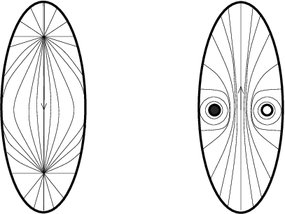
Armed with this vector field, we define the map promised in Equation (6). Fix a Morse function compatible with the Heegaard diagram . Given , consider the flowlines , , and . We replace the gradient vector field in a neighborhood of so as not to vanish there. Similarly, we replace the gradient vector field in a neighborhood of using so that it does not vanish there. In fact, arranging for to consist of arcs on , we obtain in this manner a vector field on which contains as a closed orbit. It is easy to see that this is equivalent to a vector field on which is a standard non-vanishing vector field on the boundary tori.
Lemma 3.11.
We have that
where here denotes the Poincaré duality map
Indeed, given , we have that
| (7) |
where here is the meridian for the component of , with its induced orientation from the orientation of .
Proof. The vector fields and differ in a neighborhood of . It is now a local calculation to see that (compare [21, Lemma ] for the corresponding statement for structures). It is easy to see that is homologous to .
The second remark follows immediately from Lemma 3.10.
The following fact will be useful in studying the symmetry properties of link Floer homology.
Lemma 3.12.
Let be a multiply pointed Heegaard diagram representing an oriented link , and let denote the induced map to relative structures. Then, specifies the same link, endowed with the opposite orientation. Let denote its induced map. Then, we have that
| (8) |
Also, is another diagram representing the link with the opposite orientation; let denote its corresponding map. Then,
| (9) |
Proof. For the first remark, note that if is a Morse function compatible with , then is a Morse function compatible with . It is now a straightforward consequence of its definition that if is represented by , then represents . Thus, Equation (8) follows.
For the second observation, note that the vector fields and representing and respectively differ only in a collar neighborhood of the boundary. In fact, one can see that in this neighborhood, and can be made isotopic away from a neighborhood of the meridian, where they point in opposite directions. In this way, Equation (9) follows.
3.7. Filling relative structures
Let be an oriented link. Fix a component of the underlying link. We have a natural “filling map”
This is gotten by simply viewing the relative structure on relative to as one over relative to . More specifically, if we think of as generated by vector fields which have a closed orbits consisting of the components of (traversed with their given orientations), then we can view these also as relative structures which have a closed orbits consisting of the components of (traversed with their given orientations).
Lemma 3.13.
We have the following
Proof. To verify this, let be an oriented surface in with boundary on , representing some relative homology class . We can assume that meets transversally. We can consider the surface in with boundary on gotten by deleting from . The homology class of represents the natural map .
If denotes the algebraic intersection number of with (endowed with the orientation it inherits from ) we have that
which is equivalent to the claim in the lemma.
4. Definition of Heegaard Floer homology for multi-pointed Heegaard diagrams
4.1. Heegaard diagrams for three-manifolds
For convenience, we work always with Floer homology with coefficients in . We also consider the case where the ambient manifold is a rational homology three-sphere, and hence Proposition 3.6 applies.
Let be an -pointed balanced weakly admissible Heegaard diagram for a rational homology three-sphere . We define to be the free module over the polynomial algebra generated by the intersection points inside . There is a module homomorphism
defined by
| (10) |
Here, as usual, denotes the moduli space of pseudo-holomorphic representatives of the given homology class of Whitney disks, and denotes the quotient of this moduli space by the action of . Also, denotes the expected dimension of (i.e. the Maslov index of ). (Indeed, we will find it useful later to use Lipshitz’s cylindrical formulation [14] instead; we return to this point in Section 5.)
We will establish the following in Subsection 5.3:
Proposition 4.1.
For an -pointed, balanced, Heegaard diagram for a rational homology three-sphere , for any , we have that
| (11) |
Lemma 4.2.
For an -pointed balanced weakly-admissible Heegaard diagram for a three-manifold and any , the right-hand-side of Equation (10) consists of only finitely many different non-zero terms.
Proof. First, we prove that the coefficient of in is finite, for any given . But this follows readily from the fact that for any two homology classes with , is a periodic domain, which hence must have both positive and negative coefficients. It follows from this that there are at most finitely many homology classes with and , and hence which can support holomorphic representatives.
If admits a holomorphic representative, then for all ; from Proposition 4.1, it follows at once that for with , the quantity depends only on and . Thus, given and it follows that there are only finitely many different possibilities for with non-zero coefficient on the right-hand-side of Equation (10).
Lemma 4.3.
The map is a differential on .
The above lemma is proved in Section 6, where we also prove that the homology groups are identified with the usual Heegaard Floer homology of [21]:
Theorem 4.4.
The chain homotopy type of the complex over the polynomial ring is a three-manifold invariant; indeed, its homology coincides with the Heegaard Floer homology group .
A more precise version of the above theorem can be stated, which respects the splitting of according to its various structures. We do not belabour this point now, as the primary example we have in mind here is the case where (which has a unique structure).
There is a simpler variant of the above construction, where we set , formally – i.e. we consider the free module over the polynomial algebra generated by , endowed with the differential:
It is easy to see that the arguments from Theorem 4.4 also show that the homology of this chain complex calculates .
The simplest variant counts holomorphic disks which are disjoint from all the , to obtain a complex i.e. specializing to the case where for all . Explicitly, this is the chain complex of -vector spaces spanned by the intersection points of , and equipped with the differential
For this complex, we have the following:
Theorem 4.5.
The complex calculates .
4.2. Links and multi-filtrations of
The multi-pointed Heegaard diagram for an oriented link endows the chain complex with a relative -filtration, as follows.
Let be the Heegaard diagram for an oriented link in a three-manifold with . In Subsection 3.6, we defined a map
We extend the above-defined function to generators of the chain complex of the form , using the formula
| (12) |
where here are meridians for the link (compatible with its given orientation).
Lemma 4.6.
Let be an oriented link in a three-manifold with , and consider the corresponding identification , given by , making into an affine space for . Then, the function (as defined in Subsection 3.2, and extended in Equation (12) above) induces a -filtration on the chain complex (endowed with the differential from Equation (10)).
Proof. Suppose appears in with non-zero coefficient. We must prove that then . But in this case, there is a with a holomorphic representative, and hence . On the other hand, , and hence
in view of Equation (7).
The following will be verified in Section 7:
Theorem 4.7.
The -filtered chain homotopy type of the chain complex of -modules is an invariant of the underlying oriented link.
Definition 4.8.
The -filtered chain homotopy type of the chain complex associated to a link will be denoted . The homology of the associated graded object is denoted
Explicitly, the associated graded object is generated as a -module by intersection points , endowed with a differential differential akin to Equation (10), only now we sum over those with and also . Indeed, the summand in grading is generated by symbols , where are non-negative integers and , satisfying the constraint that
The homology of this complex is the group
.
We can also set , to obtain a filtration of a chain complex which, according to Theorem 4.5, calculates of . More concretely, we consider the chain complex generated over by intersection points , endowed with the module homomorphism
| (13) |
As in the case of , the function endows with a filtration.
Definition 4.9.
The -filtered chain homotopy type of the chain complex associated to a link will be denoted . The homology of the associated graded complex is the link invariant .
More precisely, for , is the homology of the chain complex generated by with , endowed with the differential
| (14) |
In the introduction, no mention was made of relative structures; rather, link Floer homology was described as a group graded by elements of . For the case of links in , the equivalence of these two points of view is given as follows. Given an element , there is a unique relative structure with the property that
The group from the introduction, then, is the group . This convention is quite natural, as we shall see in Section 8.1 below.
In practice, it can be taxing to calculate relative structures. It is much simpler, rather, to define the link filtration on relative terms, declaring that
| (15) | if and only if |
where here is any element in , for example in the case where . (The equivalence of this with our earlier point of view is a direct consequence of Equation (7).) This determines the filtration only up to an overall shift (by an element of ), but this indeterminacy can be removed using the symmetry properties of the link invariant, cf. Section 8 below.
5. Analytic input
We will be concerned in this section with gluing results for pseudo-holomorphic disks. Consider an -pointed Heegaard diagram , and let . Given and a homology class of Whitney disk , we can form the moduli space .
Recall that these moduli spaces have Gromov compactifications, cf. [6], [15], [3], [4]. For a given moduli space of pseudo-holomorphic Whitney disks, these Gromov compactifications include possibly moduli spaces of pseudo-holomorphic Whitney disks connecting other intersection points, moduli spaces of pseudo-holomorphic spheres, and finally also moduli spaces of further degenerate disks called boundary degenerations. More formally, given a point , we let denote the space of homology classes of maps
Such a map is called a -boundary degeneration. We let denote the set of -boundary degenerations, defined analogously.
Loosely speaking, Gromov’s compactness theorem states that a sequence of pseudo-holomorphic curves representing , has a subsequence which converges locally to a “broken flow-line”, consisting of collection of pseudo-holomorphic flow-lines , a collection of - and -boundary degenerations , and finally a collection of pseudo-holomorphic spheres with
We will also find it necessary at several future points to study ends of moduli spaces as the Heegaard surface is degenerated. We turn to this more formally as follows.
5.1. Gluing moduli spaces
Let and be a pair of Heegaard diagrams, where here and are -tuples of attaching circles in . We can form their connected sum at and to obtain a new surface , endowed with sets of attaching circles and . We will assume that , and write and .
We will need here descriptions of the moduli spaces of flowlines in the connected sum diagram, in terms of moduli spaces for the two pieces.
Fix points , which in turn give rise to points , in . Fix a pair of homology classes of Whitney disks with . These can be combined naturally to form a homology class . Specifically, the local multiplicities of at each domain is the local multiplicity of at the corresponding or .
Conversely, each homology class can be uniquely decomposed as for some pair of with .
Moreover, given complex structures and on and , we can form a complex structure with neck-length as follows: find conformal disks and about and , and form the connected sum
under identifications and . As , the conformal structure on converges to the nodal curve .
Theorem 5.1.
Fix diagrams for as above, where here and are -tuples of attaching circles. Given a homology class for the connected sum of the two diagrams, we have that
where . Suppose that for a sequence of almost-complex structures with . Then, the moduli spaces of broken pseudo-holomorphic flowlines representing and (i.e. the Gromov compactifications of these two moduli spaces) are non-empty. Finally, suppose that , , and also that ; and consider the maps
| and |
where here
If the fibered product of and
is a smooth manifold, then there is an identification of this moduli space with the moduli space , for sufficiently long connected sum length.
There are three assertions in the above theorem: one concerns the Maslov index, one the existence of weak limits, and the third is a gluing result. They are arranged in order of difficulty; the third requires the most work. One could approach this problem from the point of view of degenerating as the connected sum degenerates into , following the approach to stabilization invariance from [21]. In this case, the limiting symplectic space is , which has a fairly complicated singular set (consisting of those -tuples where one element is the singular point ). In particular, the singular set is, in itself, not a symplectic manifold but rather a singular space whose singularities consist of those -tuples where at least two elements are the point . Under the present circumstances, holomorphic disks we wish to resolve – whose boundary lies from in the the top stratum – meet the singular stata (consisting of those tuples where at least one point is the singular point ) in a complex codimension one subset, i.e. where at least two coordinates agree with this singular point.
A much simpler approach can be given using Lipshitz’s cylindrical reformulation of Heegaard Floer homology, cf. [14]. With this reformulation, then, the gluing problem takes place in a four-manifold, along a singular set which is a manifold, (placing it on roughly an equal footing with the proof of stabilization invariance for cylindrical reformulation, cf. [14]). This kind of degeneration has been extensively studied in the literature, cf. [7], [13], [2], [1], and of course [14]. We turn to this approach, first recalling the basic set-up of Lipshitz’s picture.
5.2. Lipshitz’s cylindrical formulation of Heegaard Floer homology
The starting point of Lipshitz’s formulation is that a holomorphic disk corresponds to a holomorphic curve in , which, for any , meets the fiber in the set of points . Thus, one could reformulate the chain complex defining Heegaard Floer homology as counting certain pseudo-holomorphic surfaces in .
This can be made more precisely as follows. Consider the four-manifold
equipped with two projection maps
| and |
(As usual, we think of the unit disk in the complex plane as the conformal compactification of the infinite strip , obtained by adding points at infinity.) Endow with an almost-complex structure tamed by a natural split symplectic form on , which is translation invariant in the -factor, and for which the projection is a pseudo-holomorphic map. For example, the product complex structure – which will be called a split complex structure – satisfies these conditions, but it is often useful to perturb this. However, to ensure positivity, it is convenient to choose points , and require that is split in a neighborhood of (in ) times . Such an almost-complex structure is called split near .
Consider next a Riemann surface with boundary, “positive” punctures and “negative” punctures on its boudnary.
Lipshitz considers pseudo-holomorphic maps
satisfying the following conditions:
- •
is smooth.
- •
.
- •
No component in the image of is contained in a fiber of .
- •
For each , and consist of exactly one component of
- •
The energy of is finite.
- •
is an embedding.
- •
Any sequence of points in converging to resp. is mapped under to a sequence of points whose second coordinate converges to resp .
We call holomorphic curves of this type cylindrical flow-lines. Thinking of the complex disk as a compactification of , a map as above can be extended continuously to a map of the closure of into . We say that connects to if the image of this extension meets in the points and it meets in the points .
Projecting such a map onto , we obtain a relative two-chain in relative to , whose local multiplicity at some point is given by the intersection number
Conversely, given , let denote the moduli space of cylindrical flow-lines which induce the same two-chain as .
It is sometimes also useful to consider the analogue of boundary degenerations in this cylindrical context.
Definition 5.2.
Consider a Riemann surface with boundary and punctu res on its boundary. Consider now pseudo-holomorphic maps which are finite energy, smooth embeddings, sending the boundary of into , containing no component in the fiber of the projection to , so that each component of consists of exactly one component of . Such a map is called a cylindrical boundary degeneration. For such a map, the point at infinity is mapped into a fixed . These maps can be organized into moduli spaces of indexed by homology classes . A corresponding definition can also be made with playing the role of .
In [14], Lipshitz sets up a theory analogous to Heegaard Floer homology (in the case where ), counting elements of . In setting up this theory, he establishes the necessary transversality properties: for a generic choice of almost-complex structure over as above, all the moduli spaces with are empty; non-empty moduli spaces with consist of constant flowlines, and moduli spaces with are smooth one-manifolds. He also shows that these moduli spaces have the necessary Gromov compactifications analogous to those for the moduli spaces of holomorphic disks in a more traditional Lagrangian set-up. Indeed, in [14] Appendix A, Lipshitz establishes identifications for suitably generic choices of almost-complex structures, in cases where . In particular, if we consider the map defined as in Equation (10), only using moduli spaces in place of , then the two maps actually agree. Although Lipshitz considers the case where , the logic here applies immediately to prove the corresponding result in the case where , as well.
With this cylindrical formulation, now the denegeration considered in Theorem 5.1 becomes more transparent. Specifically, the degeneration of to corresponds to a generation of into and , two symplectic manifolds which meet along the hypersurface , joined along and . (Compare also [7], [13], [2], [1]. Finally, observe that this is precisely the set-up which Lipshitz uses in his proof of stabilization invariance for the cylindrical theory, see [14]).
More precisely, we start with almost-complex structures and on and and neighborhoods and of and . We assume that and which are split on and respectively. From this, we construct a complex structure on
which agrees with near , and near , and which is split over .
Definition 5.3.
A pre-glued flowline representing the homology class is a pair of cylindrical flow-lines and satisfying the matching condition
Similarly, a pre-glued -boundary degeneration is a pair of -boundary degenerations and satisfying the analogous matching condition . A similar definition can also be made for -boundary degenerations.
The curves divide into regions . Choose reference points , one in each .
It will be useful to have the following:
Lemma 5.4.
Given , we have that .
Proof. This follows readily from the excision principle for the the linearized operator, to reduce to the case of a disk. (See the proof of Theorem 5.5 for a more detailed discussion of a related problem.)
We interrupt now our path to Theorem 5.1, paying off an earlier debt, supplying the following quick consequence of the above lemma:
Proof of Proposition 4.1 According to Equation (5), the homology classes of and differ by the juxtaposition of a boundary degeneration with , whose index, according to Lemma 5.4, is given by . The result now follows from the additivity of the index under juxtaposition. ∎
We give another consequence of Lemma 5.4. By arranging for the almost-complex structure on to be split near neighborhoods of all the , one can arrange for the usual positivity principle to hold: if a moduli space is non-empty, then all the . It follows from this, together with Lemma 5.4, that if is a homology class of boundary degenerations which contains a non-constant pseudo-holomorphic representative, then . This principle is used in the following:
Proof of the cylindrical analogue of Theorem 5.1. We turn to Theorem 5.1, using moduli spaces of cylindrical flowlines in place of pseudo-holomorphic Whitney disks. In this context, the restriction maps are to be replaced by maps
given by
The formula for the Maslov index follows readily from the excision principle for the linearized operator, using the cylindrical formulation. Consider a sequence of pseudo-holomorphic curves , where here the subscript denotes the almost-complex structure induced on with neck-length as described earlier. Using Gromov’s compactness theorem, after passing to a subsequence, converges locally to a pseudo-holomorphic curve in the symplectic manifold
which in turn can be completed to a pseudo-holomorphic curve in and one in . More precisely, we obtain a broken flow-line whose components consist of pre-glued flowlines and boundary degenerations, finally also nodal curves supported entirely inside fibers . The representatives in the moduli spaces for and respectively are gotten by ignoring the matching conditions.
In the case where , the limiting process generically gives rise rise to an unbroken, preglued flowline, according to the following dimension counts. Specifically, taking a Gromov compactification, we obtain a pseudo-holomorphic representative of , and also a possibly broken flow-line representing .
Assuming that this broken flow-line contains no components which are closed curves, there is some component of it with the property that and represents a pre-glued flowline in the sense of Definition 5.3. We claim that in fact represents . If did not represent , then it represents a homology class which is a component in the Gromov compactification of . If this compactification contains additional boundary degenerations, the Maslov index of is at least smaller than the Maslov index of (in view of Lemma 5.4). Moreover, if the compactification contains other flows, those will serve only to further decrease the Maslov index of relative to that of . In sum, in the case where does not agree with , its Maslov index . But given , the moduli space
has expected dimension . Thus, for a generic choice of (gotten by ), this space is empty.
It is easy to rule out also the case that the Gromov limiting representing representing cannot have any closed components. To this end, suppose it has some components which represent the homology class for some . After deleting these components, we are left with a homology class with (c.f. Lemma 5.4). Some component of this Gromov compactification has , where is obtained from by deleting points. But the moduli space of such points has expected dimension given by
| (16) |
and hence it is empty (here, of course, is where we used our assumption that ).
Thus, we have established that a sequence of holomorphic representatives for has a Gromov limit (as we stretch the neck) to a pre-glued flowline representing and . Conversely, given a pre-glued flowline, one can obtain a pseudo-holomorphic curve in by gluing (cf. [14] for further details on this gluing problem, and [1] for a discussion of gluing in a very general context). ∎
5.3. Counting boundary degenerations
We let denote the moduli space of pseudo-holomorphic boundary degenerations in the homology class of . Note that acts on the this moduli space, and we let denote the quotient by this action. The principles used in proving Theorem 5.1 can also be used to count boundary degenerations.
Theorem 5.5.
Consider , a surface of genus , equipped with a set of attaching circles for a handlebody. If and , then for some ; and indeed in this case
| (17) |
Proof. It follows readily from Lemma 5.4 that if is a non-zero homology class of boundary degenerations with , then , with equality iff . In the case where , it remains to verify Equation (17). The case where has already been established in [21, Proposition ] for the usual Heegaard-Floer moduli spaces and [14] for the cylindrical version. Consider some region , which we re-name simply . Recall that this is a Riemann surface with boundary, equipped with curves , of which the first comprise its boundary, and the rest are pairwise disjoint, embedded circles in the interior. We have fixed also . We reduce to the case where , by de-stabilizing. Next, we reduce to the case where the number of boundary circles is one. To this end, we can write , where here is a disk with boundary , and is a planar surface-with-boundary . Denote the connected sum point in by and the one in by . Degenerating the connected sum tube, we obtain a fibered product description , where the fibered product is taken over the maps
| and |
defined as before. It is easy to see, though that is smooth, and the map is in fact a diffeomorphism. Thus, it follows that . In this manner, we have reduced to the case where and , which is, once again, the case where . Now, since the map is -equivariant, we see that is precisely the degree of the map , which is one.
5.4. Notational remark
The notation of Theorem 5.1 suggests using moduli spaces of pseudo-holomorphic Whitney disks, while its proof uses cylindrical flow-lines. One could close the gap by either appealing to an identification between the two kinds of moduli spaces, cf. [14], or simply adopting the cylindrical point of view instead; either approach has the same final outcome. In view of this remark, we henceforth drop the notational distinction between cylindrical and more traditional moduli spaces.
6. Heegaard Floer homology for multi-pointed Heegaard diagrams revisited
Having set up the analytical preliminaries, we now prove the invariance properties promised in Section 4.
Proof of Lemma 4.3. In the usual proof that from Floer homology (cf. Theorem for a proof in the original case, and [14] for the cylindrical formulation), this is observed by counting ends of two-dimensional moduli spaces.
Specifically, fix intersection points and , and a vector . We consider the ends of
In the case where , these ends cannot contain any boundary degenerations, since according to Lemma 5.4, these all carry Maslov index at least (and hence if they appear in the boundary, the remaining configuration has Maslov index , and hence, if it is non-empty, it must consist of the constant flowline alone). Thus, the ends in this case are modeled on
And the total count of these ends are given by
| (18) |
which on the one hand must be even, on the other hand, it is easily seen to be the -component of . In the case where , there are additional terms, which count boundary degenerations meeting constant flowlines, whose total signed count is
According to Theorem 5.5, this quantity vanishes. More precisely, except in the case where and is one of the components of , so that has the form that for all but one value of , where the component . In this case , but there is also a unique cancelling with and . Thus, we are left once again with a sum as in Equation (18) which can be interpreted as the -component of . ∎
6.1. Simple stabilization invariance
The aim of this subsection is to prove that the homology of the chain complex is invariant under a particularly simple index zero/three stabilizations (c.f. Proposition 3.3).
Specifically, recall that if we have a balanced Heegaard diagram with , , , we can construct a new balanced Heegaard diagram by introducing a new pair of separating curves and and a new basepoint , so that is isotopic to in . Let , , where for , resp. is obtained from resp. by a small isotopic translate. As in Section 3, we say that this new diagram is obtained from by an index zero/three stabilization.
We call the stabilization simple if bounds a disk in whose closure is disjoint from the other .
Let be the two-sphere, and be an embedded curve which divides into two regions, each of which contains a basepoint or . Let be a small Hamiltonian isotopic translate of (in the complement of and ), meeting in two points and , cf. Figure 3. Of course, represents a balanced diagram for .

Lemma 6.1.
If or with , then
| (19) |
Moreover, the chain complex is given by
For the claim about the chain complex, it is easy to see that boundary maps from to come in cancelling pairs, whereas there are two holomorphic disks from to with Maslov index one, and they are bigons, one of which contains the other .
Definition 6.2.
Let and be a pair of balanced multi-pointed Heegaard diagrams, and choose basepoints , . We can form their connected sum , a balanced -pointed Heegaard diagram whose underlying surface is obtained from and by forming the connected sum at the points and . We let , , only now thought of as curves in , and , where is some reference point on the connected sum neck. We denote this connected sum by .
In particular, given an arbitrary multi-pointed the Heegaard diagram , a simple index zero/three stabilization can be thought of as the connected sum with as considered in Lemma 6.1.
Fix a Heegaard multi-diagram , choose , and . Correspondingly, let , where , denote the map which assigns to the Whitney disk the divisor or, in the cylindrical formulation, . Given and , we let denote the moduli space of pseudo-holomorphic maps representing with the additional constraint that .
Lemma 6.3.
Let be a homotopy class of Whitney disks for a balanced Heegaard diagram . If , then is generically a zero-dimension moduli space. Moreover, there is a number with the property that for all , the only possible non-empty moduli spaces with consist of moduli spaces for with , and indeed is obtained by splicing a boundary degeneration to the constant flowline. Indeed, for this moduli space,
Proof. The dimension statement is clear. Note that the admissibility hypothesis ensures that there are at most finitely many consisting of moduli spaces for with and , and hence only finitely many homotopy classes for which could possibly be non-empty for some . Consider one such homotopy class, and suppose that is non-empty for a sequence of . Let be a corresponding sequence of pseudo-holomorphic curves. Taking their Gromov limit, we obtain a broken flow-line representing the homology class . Since contains points arbitrarily close to the line but does not lie in any of the , we can conclude that the Gromov limit must contain a component which is a non-trivial boundary-degeneration . According to Lemma 5.4, we can conclude that . Thus, the remaining configuration has non-positive Maslov index, and it also has a pseudo-holomorphic representative. This forces it to be a constant flowline.
We have thus established that there is a real number such that if is non-empty for any , then is obtained by splicing a boundary degeneration to a constant flowline. The result now follows by gluing to the constant flow-line, and applying Theorem 5.5.
We will also need a result about a suitable generalization of , but only for the Heegaard diagram introduced above.
Given a divisor , let
Lemma 6.4.
Consider the Heegaard diagram as above, with the two intersection points . Fix also a generic for some positive integer . Then,
for or .
Proof. Consider the case where . Let . We claim first that depends on only through its total weight . Specifically, if are two generic points in , then . This follows from the following Gromov compactness argument. Let be a path in connecting and . Consider the one-dimensional moduli space
This has four types of ends. The first type appear in the expression
The total number of such ends is zero, since is a cycle (in the chain complex for ). The second type of ends appear in
The total number of such ends is zero, since is a cycle. Note that or for any such degeneration, since otherwise our divisor family remains in a compact portion of the interior of the disk for all .
The third and fourth types of ends appear in
and the related expression
Thus, taken together, the total number of ends is given by , which must therefore vanish.
Now let consists of points each of which have horizontal component (chosen as in Lemma 6.3), and with vertical spacing of at least between them. Taking a limit as , we see that the ends of the parameterized moduli space
consist of (the end where ), and a product , in the notation of Lemma 6.3. Combining this observation with the result of that lemma, we see that .
The case where follows similarly.
Proposition 6.5.
Suppose that is obtained from by a simple index zero/three stabilization. Then, there is an identification of -modules
Indeed, multiplication by is identified with multiplication by .
Proof. We show that for suitable choices of almost-complex structures, is identified with the mapping cone of a map
| (20) |
where here denotes the chain complex
We degenerate the Heegaard surface, to realize it as a connected sum
(with sufficiently large connected sum neck) where now is identified with ; or more precisely, and are the corresponding connected sum points, and we choose a new distinguished point to lie in this connected sum region. Note that here is given by . We will use a complex structure on the connected sum surface with a very long connected sum length (and in fact, we will move the connected sum point close to the circle in , as explained below).
Clearly, ; i.e. intersection points come in two types (containing and ), and differentials can be of four types. Write resp as the submodule generated by intersection points containing resp ; i.e. we have a module splitting .
We begin by considering the -component of the differential of a generator in . Apply Theorem 5.1 to some homotopy class , in the case where . Writing , we have that
If , then (since has a pseudo-holomorphic representative). As an easy consequence of Lemma 5.4, it follows that , with equality iff . In the case where, we force , and hence it is generically empty. Thus, we are left with the case of , and . In this case, Theorem 5.1 shows that the -component of is given by
In this expression, we consider as an actual map (rather than only one modulo re-parameterization) by taking the representatives with the property that the projection of onto the factor contains , and no positive real number. According to Lemma 6.4, then, for each ,
Thus, the component of is identified with the component of for the original Heegaard diagram.
Thus we have identified the component of the differential of an element in with the differential coming from the obvious identification of with the chain complex for the original diagram . In the same manner, the differential within is identified with the differential of the original diagram.
We consider now the -component of the differential of a generator in . Again, we expresss as a fibered product over with . Now, an application of Lemma 5.4 shows that if , then , with equality iff . In the case of equality, we have that , and hence it must be constant. This forces to be one of the two flows from to with and . Each of these homotopy classes admits a unique holomorphic representative, and hence the differential cancels: the component of the boundary of something in is trivial.
Finally, we consider the component of the differential of a generator in . Splitting a homotopy class in the fibered sum description, we once again have
and hence the condition that (which is needed for its corresponding moduli space to be non-empty) translates into the condition that . Moreover, for with , we have that . Parity considerations exclude the possibility that the quantity equals .
In the case where , we conclude that , and hence it must be constant, forcing . Thus, must be the unique homotopy class with , , , and . Thus, the corresponding component of is (note that in the connected sum diagram, the reference point corresponds to the new variable ).
In the remaining cases, and . Since , we conclude that , while the condition that and readily forces .
Suppose that . In this case, is constrained to be a homotopy class with a unique holomorphic representative up to translation. Let be a holomorphic representative of , and . Note that this consists of a single point up to translation in ; after suitable translation, we arrange for . We wish now to apply Theorem 5.1, with now playing the role of in the statement of that theorem. For this, we need to assume that , the number of marked points , is greater than one (so that we are taking more than the symmetric product of , as required in the hypothesis of the last part of Theorem 5.1). We return to the case where at the end of this proof.
Completion of the proof of the proposition when . According to Theorem 5.1, count of points in all Maslov index one moduli spaces , where has is given by the map
defined by
in the notation of Lemma 6.3. By choosing sufficiently close to , we can arrange for to be arbitrarily close to . According to Lemma 6.3 for suitable choice of , this count is given by
| (21) |
There are in principle other terms which count homotopy classes with (and corresponding to factorizations of as and with , ). Our claim is that for a sufficiently large parameter , these homotopy classes have trivial contribution. Here, parameterizes the choice of connected sum point in , with the limit given by a point on the curve . Note that we have already taken large to apply Lemma 6.3 in establishing Equation (21).
Suppose now that for a sequence of going to infinity, the moduli spaces are non-empty for all choice of connected sum neck length. Then, for all sufficiently large , the fibered product is non-empty, where here .
Thus, we obtain a sequence of pseudo-holomorphic representatives of the fibered product. Clearly, there are Gromov limits and as of the curves and . By dimension counts, since , there are only three possible types of limit for : either it is a strong limit to a pseudo-holomorphic disk, or it is a weak limit to a singly-broken flowline, or it contains a boundary degeneration, in which case the remaining component must be a constant flowline. In this latter case, , and hence it has been covered earlier.
Suppose that the limit is not a broken flowline, and let denote the matching component of (i.e. could a priori be a broken flow-line, but it has some component with the property that . However, since limits to , we see that contains some points on the -boundary. To achieve this, we must have a sequence with arbitrarily large , with containing points arbitrarily close to the line . According to Lemma 6.3, this forces , a case considered earlier.
In the remaining case, the Gromov limit is given as a broken flow-line . Again, by simple dimension counts, we see that . There is also a corresponding . Since is odd, we can conclude that so is either or . Suppose it is which is odd. It is easy to see that for contains points on the boundary . Moreover, the same reasoning as before, with and playing the roles of and respectively, shows that is supported in a homotopy class which admits holomorphic representatives with containing points arbitrarily close to . But this is impossible, as is disjoint from , and has to be one of finitely many holomorphic disks up to translation. The case where is odd follows mutas mutandis.
Putting the above facts together, we obtain the desired identification of with the mapping cone of Equation (20), giving an expression
at least in the case where .
Proof of the proposition when . In this case, Theorem 5.1 cannot be applied directly to identify the component of .
Specifically, consider a homology class of , with , , and . Take a Gromov limits of elements of , as the connected sum is degenerated. Again, this limits to the unique (up to translation) holomorphic representative of , but now we cannot assume that the Gromov limit from the other side is a flow-line. More specifically, the dimension counts (cf. Equation (16)) which ruled out the possibility of a closed component in the Gromov compactification no longer apply. Indeed, by pushing the connected sum point sufficiently close to , we can use Lemma 6.3 to rule out the case where the component of in the Gromov compactification which matches with is an actual cylindrical flow-line. Rather, it must be a closed holomorphic curve representing the homology class (with multiplicity one). The argument from stabilization invariance as in [14] applies now to show that . More precisely, the Gromov limit equals a constant flow-line meeting a copy of , with . In this case, gluing can be used to show that , where here is the count of representatives with a marked point to in the homology class which maps to . The fact that , in the case where is calculated in the proof of stabilization invariance of cylindrical Heegaard Floer homology (cf. Appendix B of [14]). One can show that for arbitrary follows from this case by, for example, by realizing as a connected sum of copies of a genus one surface, and degenerating along all the necks. Now, follows from the elementary calculation that .
Thus, we have computed that the counts of all Maslov index one moduli spaces of the form , where is the flowline with is given by the same map as in Equation (21). We can rule out the case where and much as before. Specifically, by pushing the connected sum point close to , Lemma 6.3 shows that the corresponding Gromov limit must contain at least one closed curve component. Removing this component, we are left with a broken flow-line with Maslov index zero, and hence, a constant flowline, hence showing that we needed to be in the case where . The argument is now completed as before.
6.2. Model calculations
The aim of the present subsection is to continue with the methods from the previous subsection to perform some model calculations which will be useful for establishing handleslide invariance.
Definition 6.6.
Let be a chain complex over the polynomial algebra . We say that it is of -type if for , there are chain homotopies (thought of as endomorphisms of ).
Of course, if a chain complex is of -type, then its homology is a module over the polynomial algebra , where acts by multiplication by any of the .
Let be a Heegaard diagram, and fix two preferred basepoints . Let be a surface obtained by attaching a one-handle in the neighborhood of and , and fix a pair of circles and which are supported inside the handle, each a small isotopic translate of one another, separating and . Equivalently, we form a double-connected sum of along and with the sphere as in Figure 3.
Proposition 6.7.
Let be a Heegaard diagram, and let be the Heegaard diagram obtained by attaching a one-handle in the above sense, so that if the original describes a three-manifold , then the second diagram describes . Suppose that of -type, then the same is true of ; and indeed .
Proof. We analyze as in Proposition 6.5, only this time stretching near both and . In this case, homotopy classes break as fibered products of homotopy classes for , and for . Now we have
The same dimension counts as in the proof of Proposition 6.5 express as a mapping cone of a map
| (22) |
As in the proof of that proposition, the first chain complex is identified with and the second with . The map counts those disks which have . By moving the connected sum points as in Proposition 6.5, we can arrange that these terms contribute trivially.
Thus, since , the chain map from Equation (22) is null-homotopic, and it follows at once that is chain homotopic to the direct sum of two copies of .
Let be an oriented two-manifold, and be a collection of attaching circles, and let be a collection of basepoints, one in each component of . Let be a set of attaching circles obtained as small exact Hamiltonian translates of . Specifically is obtained as an exact Hamiltonian translate of , so that unless , in which case the intersection consists of two points of transverse intersection. Moreover, the Hamiltonian isotopy never crosses any of the . Clearly, represents , where is the genus of .
Proposition 6.8.
is of -type, and its homology is isomorphic to , where is a -dimensional vector space.
Proof. We can reduce to the case where by repeatedly applying Proposition 6.7. In the case where , the proposition is proved after repeated applications of Proposition 6.5.
As an example, suppose that is an admissible multi-pointed Heegaard diagram, and suppose that is obtained from by a small perturbation as in Proposition 6.8. According to Proposition 6.8, there is an element of maximal degree.
We can define a corresponding map
by
This map is a chain map (compare [21, Section ]). (In this notation, we implicitly assume that is represented by a single intersection point ; more generally, our map is gotten by summing triangle maps over the various intersection points whose sum represents the homology class.)
Proposition 6.9.
If the curves in are sufficiently close to those in , chosen so that each meets in precisely two intersection points, then the map defined above induces an isomorphism in homology.
Proof. This follows as in [21, Proposition ]. The point is that for each , there is a corresponding nearest point , and also a corresponding small triangle . Thus, the map obtained by counting only these smallest triangles induces an isomorphism of chain groups. Using the energy filtration, it follows that is an isomorphism of chain complexes.
6.3. Handleslide invariance
We can now adapt the proof of handleslide invariance of Heegaard Floer homology as in [21, Section ] to establish handleslide invariance of in the present context.
Specifically, start with a Heegaard diagram . Let be obtained from by a single handleslide.
Proposition 6.10.
There is an identification .
Proof. As a first step, we claim that , where is a -dimensional -vector space. To see this, de-stabilize using Propositions 6.5 and 6.7 to the case where there are exactly two curves and two curves. There are three cases, according to whether is , , or . The case where is established in [21]; the other two cases are easily established by the same calculation.
With this said, there is a canonical top-dimensional generator of . The handleslide map
is defined by counting pseudo-holomorphic triangles: ; i.e. here
Now, according to associativity of the triangle maps, we see that the composite
Next, we verify that is the canonical top-dimensional generator of , which is calculated in Proposition 6.8; i.e. we obtain the map studied in Proposition 6.9. The map is an isomorphism now according to that proposition.
6.4. Invariance
We prove the invariance of as introduced in Section 4.
Proof of Theorem 4.4. We show that is invariant under the four Heegaard moves from Proposition 3.3, or, more specifically, their admissible versions as in Proposition 3.6.
Isotopy invariance follows exactly as in [21, Section ].
Handleslide invariance was established in Proposition 6.10.
Invariance under index one and two stabilizations follows from exactly as in [21, Section ].
Finally, it remains to consider invariance index zero/three stabilizations. In this case, we introduce a new pair of (isotopic) curves and , each of which separates in two. In the case where the stabilization is simple in the sense of Subsection 6.1, i.e. bounds a disk containing and none of the other (or ), invariance is established in Proposition 6.5. It is easy to see that general index zero/three stabilizations can be achieved by simple index zero/three stabilizations, followed by a sequence of handleslides. ∎
The case of can be handled more quickly:
Proof of Theorem 4.5. Let be the multi-pointed Heegaard diagram, with . Let be a planar suface with boundary components. Form the surface . Consider , where here is chosen in the region . It is easy to see that is a pointed Heegaard diagram for . Admissibility of the original diagram corresponds precisely to admissibility for this new diagram. Moreover, the intersection points of in are identical with those in . Finally, holomorphic curves in which are disjoint from all the are identical with those in which are disjoint from . The result now follows. ∎
7. Invariance of link invariants
Invariance of the filtered chain homotopy type of the link filtration is an easy consequence of the methods from Section 6.
Proof of Theorem 4.7. We must verify that is invariant under isotopies and handleslides supported in the complement of and , and also index one/two stabilizations.
If is obtained from an index one/two stabilization, then the methods from Section of [21] actually give an isomorphism of chain complexes . Performing the stabilization away from and , we see that the assignment to relative structures is unaffected.
Handleslides amongst the are understood as follows. As before, if is obtained from by a handleslide, then there is a chain map (c.f. Proposition 6.10)
defined by counting holomorphic triangles. Since all triply-periodic domains are disjoint from and , it follows easily that if , then . We thus consider the induced map on the associated graded object, i.e. the map induced by counting pseudo-holomorphic triangles which are disjoint from and alike. Note that
where here is the map associated to the Heegaard diagram , since the triangles used in the definition of this count are disjoint from and . Now, adapting the argument from Proposition 6.10, we have that the map
is an isomorphism. Specifically, here
The fact that this is an isomorphism follows readily as in Proposition 6.9, with the observation that the small triangles considered there do not contain any of the the basepoints . Since induces an isomorphism of -graded complexes, it follows formally that induces an isomorphism of -filtered complexes. ∎
7.1. Link homology as an associated graded object
We consider now the link filtration.
Proof of Theorem 1.2. From its construction, we see that is the homology of the graded object associated to a -filtration of , which, according to Theorem 4.5, calculates . But is identified with the exterior algebra of (cf. for example [21, Lemma ]). Invariance of the spectral sequence is a consequence of Theorem 4.7. ∎
Proof of Theorem 1.5. Fix . Recall that the chain complex computing consists of symbols , where are non-negative integers and , satisfying the constraint that
This set is endowed with the differential as in Definition 10, except that now we sum over only those with . The further filtration on is given by the map . Its associated graded object is clearly the one stated in the theorem. ∎
7.2. Forgetful functors
Let be an -component oriented link, which we assume to be in for simplicity. Distinguish a component , and consider the filling map
studied in Subsection 3.7. Under this map, a -filtered chain complex can be viewed as a -filtered chain complex.
Let be the rank two graded vector space with one generator in grading and another in grading .
Proposition 7.1.
Let be an oriented, -component link in , and distinguish the first component . Consider the filtration , viewed as a -filtered chain complex, via the filling map using the distinguished component of . The filtered chain homotopy type of this complex is identified with .
In more elementary terms, a -filtered chain complex can be viewed as a -filtered one, by forgetting the first term in the relative filtration. The above proposition says that for the relatively -filtered chain complex , if we forget the first term in the relative filtration, we obtain the relatively -filtered complex .
In particular, if we consider the higher differentials inducing a chain complex on (from Theorem 1.2) and take their homology in the first component (in the sense of Subsection 2.1), we obtain (up to some overall translation of the grading by relative structures).
Proof of Proposition 7.1. We begin with the relative -filtered statement.
In view of Propositions 6.5 and 6.7, and keeping track of filtrations, we see that the -filtered chain complex obtained from obtained by forgetting about the first factor is identified with the mapping cone of
where and is some integer . This identification is gotten by reducing to the case of simple stabilizations (in the sense of Subsection 6.1), after handlesliding across the basepoint .
Specializing to for all , we obtain two copies of , verifying the simplified statement of Proposition 7.1, using only the relative -filtered statement.
To obtain the version stated here, we must add the following observations. If is a multiply-pointed Heegaard diagram for , and , then the map obtained by handlesliding across still preserves . Moreover, in the identification of Proposition 6.5 between the complex obtained from applying the forgetful map to and the complex , we have an identification between the induced relative structures. ∎
8. Symmetry
We consider the symmetry properties of . The properties we give here are formally analogous to corresponding properties of knot Floer homology, cf. [20], [24] (compare also [21]).
Proposition 8.1.
Let be an oriented link. Then, we have an identification
Proof. Suppose is a pointed Heegaard diagram representing . Then, is also a pointed Heegaard diagram for the link , only now it represents the opposite orientation . The two Heegaard diagrams give assignments
| and |
respectively. Let denote the chain complex whose homology is , i.e. this is the associated graded object for the link filtration of . Explicitly, its generators are , and it is endowed with the differential from Equation (14).
Of course, the generators for and coincide. Indeed, by pre-composing with a reflection on the disk, we see that the differentials for the two chain complexes coincide.
However, , as in Lemma 3.12. The result follows.
Proposition 8.2.
Let be an oriented link in . Let be the map defined as follows. Writing
we have that . Then, we have an identification
Proof. Write . As in Lemma 3.12, we see that and are Heegaard diagrams for and respectively. The generators of and the differentials coincide, but the two maps to relative structures differ, with . Thus, we see that there is a function with the property that
Suppose that , then there is a flowline with and , , . Now, in , it follows that , whereas for , (where here we use to denote the grading induced on the second diagram). It follows at once that there is some constant (depending on the oriented link) with the property that for all , .
Combining the above remarks with Proposition 8.1, we have that
| (23) |
There is a natural map
since the notion of equivalence classes of nowhere vanishing vector fields does not refer to the orientation of the ambient manifold. Note, however, that , since the induced two-plane field on gets opposite orientations depending on the orientation of .
Proposition 8.3.
Let be an oriented link, and let denote its mirror. Then,
Proof. If represents , we can think of as representing its mirror. It is easy to see that this latter chain complex is the dual complex for the former, i.e.
so that the assignment from the intersection points to relative structures is intertwined with the natural map referred to above. The shift in grading follows from the fact that both total complexes for have homology isomorphic to , graded so that its top-most term has grading (cf. Theorem 1.2).
8.1. Notational remarks
Relative structures are not very concrete objects, and hence it is sometimes awkward to describe link Floer homology as filtered by them. We could alternatively use relative two-dimensional homology, and indeed the above results suggest the following convention.
For , we could define to be , where here is the relative structure determined by the formula
Given , write
We let be the quantity
With these conventions, then, Proposition 8.2 reads
It is simpler yet to consider as graded by elements of ; i.e. given , write , where is chosen so that
| (24) |
Now, Proposition 8.2 reads
| (25) |
Note that we could have had the grading set be inside , rather than , by dropping the factor of in Equation (24). However, we have chosen the present formula so that , in the case where is a (one-component) knot.
9. Euler characteristics
The aim of this section is to calculate the Euler characteristic of link homology, establishing Equations (1) and (2).
9.1. The case of
Let be a connected, -dimensional CW complex, and let . The Reidemeister-Franz torsion of is defined as follows (see for example [16], [28]). Let denote the field of fractions of the group-ring . Let denote the covering space determined by the natural homomorphism of . The action by gives the CW complex of , a complex of free -modules. In particular, its differentials
are all -equivariant. A fundamental family of cells for is a a collection of cells for , each of which projects to exactly one cell of . The Reidemeister-Franz torsion is defined to vanish if . Otherwise, we proceed as follows. Suppose that and are two ordered bases for some vector space. Then, their top exterior products differ by an element which we denote by (i.e. ). Let be a sequence of vectors in whose image under forms a basis for this image. By our assumption, is a basis for ; let be a basis for coming from a fundamental family of cells for . Then, the Reidemeister-Franz torsion is defined to be
In the case where is the complement of an -component link , , and . Indeed, in this case the Reidemeister-Franz torsion, which we now denote by , is related to the (multi-variable) Alexander polynomial by the formula
Although this defines only up to an overall sign and translation by elements of , the latter indeterminacy can be resolved by taking the representative of which satisfies the symmetry , where here is the map induced by taking to . (The existence of such a symmetric representative is standard in the theory of torsion, cf. [16], [28].)
Proposition 9.1.
Given a link , we have an identification
| (26) |
(Here, we think of , where are meridians for .)
Proof. Let be a -pointed Heegaard diagram for subordinate to .
By stabilizing if necessary, we can arrange for the following conditions to hold:
- •
the genus of is , with forming meridians for the various components of ,
- •
there are circles , with the property that for and is empty unless , in which case and meet in a single point.
- •
and can be connected by an arc which is disjoint from all the with , and it is also disjoint from all the with , meeting transversally in a single point.
Let be the one-handle in corresponding to the circle , and be the two-handle corresponding to the attaching circle . The zero-handles , the one-handles , and the two-handles together form a handle decomposition for . Let , , and (with , , ) denote a collection of lifts to the cover . Note that we can label so that
| (27) |
for all .
Observe next that for any , we have that
This establishes Equation Equation (26), up to an overall translation by units in the Laurent polynomials in . The indeterminacy in translation by the various is resolved by observing that both sides of the equation are symmetric under the involution of the ring of Laurent polynomials induced by (for all ): the left-hand-side is invariant according to Proposition 8.2, while the right-hand-side is symmetric by basic properties of torsion, cf. [16].
9.2. The case of
Proposition 9.2.
We have an identification
Proof. Each generator gives rise to infinitely many generators
for all , with . Thus, it follows that
Since
the proposition now follows from Proposition 9.1.
10. Relationship with knot Floer homology
Our aim here is to show that certain aspects of the link Floer homology considered here can be extracted from the knot Floer homology of links considered in [20]. Specifically, we prove Theorem 1.1, which shows in particular that the total rank of agrees with the total rank of the knot Floer homology for an oriented link. From this, we quickly deduce the link Floer homology of alternating links, in Subsection 10.1.
First, we briefly recall the construction from [20]. Suppose that is an -component oriented link in . Then, we can construct an oriented knot in as follows. Fix points in which are paired off in such a manner that if we formally identify each with in , we obtain a connected graph. We view and as the feet of a one-handle to attach to . Attaching all of these one-handles, we obtain a three-manifold which is diffeomorphic to . Inside each one-handle, we can find a band along which to perform a connected sum of the component of containing with the component containing . We choose the band so that the induced orientation of its boundary is compatible with the orientation of the link (moreover the band is chosen to be always transverse to the foliation of the one-handle by two-spheres). Our hypotheses on the number and distribution of the distinguished points ensures that the newly-constructed link gotten by performing all of the connected sums is in fact a single-component knot. We denote this link by inside . It is not difficult to see that the diffeomorphism type of the pair depends on only the underlying oriented link (cf. [20, Proposition ]); hence we denote this object simply by the knot .
With these preliminaries, the knot Floer homology groups
of an oriented link are defined to be the knot Floer homology groups of :
In our proof of Theorem 1.1, it will be useful to pass from a Heegaard diagram for a link to a corresponding Heegaard diagram for . This is done as follows. Fix a Heegaard diagram for an oriented, -component link . Write , . We attach one-handles to to obtain a new surface as follows. The feet of the one-handle is attached along a neighborhood of and . Letting and , we get a two-pointed Heegaard diagram for (compare the proof of Theorem 4.5). Admissibility for translates into admissibility for .
Proof of Theorem 1.1. There is a one-to-one correspondence between generators for and .
Collapse the relative filtration on to a relative -filtration by
where here is any Whitney disk in . Recall also that the -filtration on is given by
where here is any Whitney disk in .
Clearly, any Whitney disk in gives rise naturally to a Whitney disk in , having the property that for . From these conditions, it is immediate to see that
identifying one of the factors in the bigrading for both theories.
Moreover, it is also straightforward to see that , and hence the relative homological gradings of both theories are identified. A shift in the absolute homological bigradings by can be identified in a model calculation, according to which the top-dimensional generator generates in the corresponding multiply-pointed Heegaard diagram. We can also remove the indeterminacy in the relative -filtration, using the fact that both theories are enjoy the symmetry property (Proposition 8.2).
Having established that both complexes have the same generators with the same bigradings, it remains to show that the differentials are identified; i.e. for suitable choices of complex structure on , the holomorphic disks correspond, as well.
By stabilizing and renumbering curves if necessary, we can arrange for the diagram to have the following properties:
- •
for positive, odd less than or equal to , an are connected by an arc which meets in a single point but which is disjoint from all the other and ,
- •
for positive, even less than or equal to , an are connected by an arc which meets in a single point but which is disjoint from all the other and ,
Our aim is to exhibit a complex structure on with the property that for all and all with and (i.e. these are the disks which contribute in the differential for ), if is non-empty, then we must have for all , as well.
The complex structure is obtained by thinking of as obtained from by adding one-handles with a long connected sum length attached connecting to (for ). We choose the feet of these handles and in a family and starting out at and our original and respectively, , for odd less than ,
while for even ,
This can be achieved by constraining and to be subarcs of .
We have a two-parameter family of complex structures on , , where denotes the conformal structure on the annulus in the connected sum region, and parameterizes the placement of the feet of the one-handles and .
Starting with our homotopy class , thought of representing a cylindrical flow-line in , let be the corresponding Whitney disk in . If for all , we can find sufficiently large for which is non-empty, then we can take a Gromov limit (as ) for any choice of . This gives a possibly broken pseudo-holomorphic cylindrical flow-line representing .
Observe that since , it is clear that contains no components which contain all of . Moreover, it can contain no boundary degenerations. Specifically, each boundary degeneration satisfies for all , while a boundary degeneration arising in this manner must also satisfy the additional conditions that (as ), forcing all . This forces .
Thus, represents a juxtaposition of cylindrical flow-lines in . Moreover, each component in the Gromov compactification must satisfy the conditions that
for , while . Indeed, the same remarks apply taking , as well: we obtain a possibly broken flowline , each of whose components onsist of cylindrical flowlines satisfying
| (28) |
Choose minimal with the property that . If there is no such , of course, then represents a flowline with all as desired. Otherwise, we assume that (returning to the other case later). Then, some component of has . In fact, if is odd, then is contained in . However, since is not on one of the -circles, is disjoint from , contradicting Equation (28). A symmetrical argument applies when is even. In the other case, where , we can instead find the minimal for which , and then apply similar reasoning to derive a contradiction. ∎
10.1. Alternating links
11. The Künneth formula for connected sums
In this section, we study the behaviour of the link invariant under connected sums, generalizing corresponding results for knot Floer homology (cf. [20], [24]). We give a variant for the filtration of , and use it to conclude a corresponding result for (Theorem 1.4).
Let be a filtered chain complex over the ring and be a -filtered chain complex over , we can form their tensor product , thought of as a chain complex over the polynomial ring . This complex is naturally -filtered, by the rule that the part of in filtration level , , is generated by the sum over all of the subcomplexes
Consider two links and , and fix components , . There is a natural map
defined as follows. Represent relative structures and as nowhere vanishing vector fields and which are tangent to and respectively. Deleting a sufficiently small ball around , the vector field points normal to the boundary at exactly two points, where the corresponding component of meets . Find a corresponding ball around . We can then identify with , and hence extend the vector field over , to obtain a nowhere vanishing vector field containing as a closed orbit. This determines the stated map. It is easy to see that
where here
are the natural maps.
We can refine the above tensor product as follows. If is a -filtered complex over and is a -filtered one over , we can form the chain complex complex
equipped with the -filtration, where
is generated by the sum of over all pairs and with .
Theorem 11.1.
Let and be oriented links with and components respectively. Fix also a point and , and form the connected sum (near the two distinguished points). Then, the chain complex is isomorphic (as a -filtered chain complex over ) to the tensor product , where here and are variables corresponding to the components of and distinguished by the points and respectively.
Proposition 11.2.
Let and are links with multi-pointed Heegaard diagrams . The connected sum , where we connect the first component of with the first component of , can be given a Heegaard diagram
whose underlying surface is formed by the connected sum of and along the point and . In this new diagram, the pair of reference points and represent the connected sum of the first component of with the first component of .
Proof. Straightforward.
Proof of Theorem 11.1. Let , , and be small perturbations of the sets of curves , , and respectively. Correspondingly, there are canonical top-dimensional intersection points and .
We have a map
Combining Propositions 6.5 and 6.7, we see that this is a chain map. There is a similar map
defined by
Finally, we have a chain map
defined by counting pseudo-holomorphic triangles.
Putting these together, we obtain a composite chain map
There is also a “closest point map” inducing an isomorphism of modules over the polynomial algebra ()
with . Here is the point nearest to , while is the point closest to . The closest point map can alternatively be thought of as counting holomorphic triangles with minimal area. Thus, is a map of the form plus lower order terms (provided that the curves resp. are sufficiently to resp. ). In particular, induces an isomorphism of chain complexes over .
It is easy to see that
Thusm the map induces an isomorphism on the associated -graded complex. The other terms in have lower order than , and hence induces a -filtered isomorphism, as claimed. ∎
12. Examples
We turn to some sample calculations. Specifically, we will be concerned here with calculation the filtered chain homotopy type of for various oriented links. In Subsection 12.1, we give a theorem which can be used to compute this data explicitly for a two-bridge link. In Subsection 12.2, we give some calculations of this data for the first two non-alternating links.
12.1. Two-component alternating links
Although Theorem 1.3 concerns only the homology of the associated graded object , in many cases, one can also use it to deduce information about the filtered homotopy type of the full chain complex.
We study here the filtered chain homotopy type of alternating links. For simplicity, we consider here the case of two-component links.
Theorem 12.1.
Let be an oriented, two-component link which admits a connected, alternating projection. The filtered chain homotopy type of is determined by the following data:
- •
the multi-variable Alexander polynomial of
- •
the signature of
- •
the linking number of and
- •
the filtered chain homotopy type and of the two components and of .
In the course of the proof, we show explicitly how is determined by the data. First, we must set up some notions.
We say that a -filtered chain complex is -collapsed if it has a splitting so that its differential is written has the form , where here
| and |
For example, suppose that is a filtered chain complex which also has an internal grading (which the differential drops by one). Suppose moreover that the filtration and the grading are related by for some constant . Then, is collapsed. Theorem 1.3 ensures that the link Floer homology of an alternating link is -collapsed.
We give some examples of -collapsed chain complexes. Let denote the chain complex with
and the property that and and and are field isomorphisms.
Fix an integer , and let be the chain complex with
where is a sum of maps, where are field isomorphisms for all , is an isomorphism for all .
Similarly, let be the chain complex with
where is a sum of maps, where is an isomorphism for all , while is an isomorphism for all .
Note that .
There are two basic types of -collapsed chain complexes with non-trivial homology Let be the complex given by
where is a sum of maps, where and are isomorphisms when and , and zero otherwise.
Also, let be the complex determined by
where is a sum of maps, where is an isomorphism when , , and , while is an isomorphism when , , and , and all other maps are zero.
For these latter two complexes, we see that .
It is straightforward to see that for each -collapsed chain complex is filtered chain homotopy equivalent to a filtered chain complex which splits as a direct sum of copies of chain complexes of the type , , , and , allowing , , and to vary. (Here, as in Section 2, given a -filtered chain complex, we let denote the filtered chain complex obtained from by shifting the filtration, so that .).
Proof of Theorem 12.1. In view of Theorem 1.3, is an -collapsed chain complex, and as such decomposes into summands of the above five types. Thus, the filtered chain homotopy type is determined by the number of summands of each type, and their various parameters (, , , and in four cases, ). Our goal is to show how the data assumed in the statement of Theorem 12.1 can be used to extract all of the needed information.
Let denote the -filtered chain complex
endowed with a differential which is an isomorphism from to . It is easy to see that each -filtered chain complex splits as a sum of complexes of the form , and also homologically non-trivial complexes of the form supported in some fixed degree and filtration level.
Observe that taking the homology in the vertical direction (i.e. taking the homology with respect to to obtain a -filtered chain complex, endowed with the differential induced from ) has the property that it annihilates , . Moreover, taking the vertical homology of , we obtain . The vertical homology of is a copy of in filtration level , while the horizontal homology gives in filtration level ; the horizontal homology of is a copy of in filtration level while its vertical homology gives in filtration level .
On the other hand, according to Proposition 7.1, if we take the vertical homology of , we obtain the knot filtration on coming from , tensored with (supported in two consecutive dimensions) and shifted over (in its filtration) by , and taking the horizontal homology, we obtain the knot filtration of again shifted by and tensored with . Specifically, these two projections are -filtered chain complexes, and as such can be decomposed into one-step complexes (supported in some filtration level), and two-step complexes , consisting of in filtration level and (trivial otherwise), endowed with a differential which induces an isomorphism from the part in filtration level to the one in filtration level .
It follows from the above remarks that the summands in of the form are in two-to-one correspondence with the summands of type in : more precisely, if appears in , there are two summands, , and also . Similarly, the summands in of the form are in two-to-one correspondence with the summands of type in : more precisely, if appears in , there are two summands, , and also .
Moreover, since , there can be at most two summands of type or . We claim that there are in fact only two possible cases: either the two summands are and or and . This follows from the constraints that are supported in two consecutive degrees ( and ), together with the constraint that if we take the horizontal resp. vertical homologies, we are to get a filtered chain complex whose homology is supported in two consecutive gradings and the same filtration level. In fact, taking the vertical resp. horizontal homology gives the knot Floer homology of resp. , tensored with , supported in two consecutive dimesions and filtration level resp. .
More specifically, writing , , and for the linking number of with , we have two cases, according to the sign of
If , has summands
If , then has summands
The remaining summands of type (and their precise placement) are determined by the Alexander polynomial of . ∎
For example, if is a two-component, two-bridge link, Theorem 12.1 applies immediately to express the knot filtration in terms of the Alexander polynomial and signatures of . Note in particular, that in this case, the two components and are individually unknotted; it follows in particular that there are no summands of type or . (Any two-bridge link can be represented by a four-pointed Heegaard diagram with genus zero, and hence the holomorphic curve counts defining the differential take place in the Riemann sphere. Thus, these counts are purely combinatorial, compare [23] and also [20, Section ].)
Consider the Hopf link . There are two orientations for , distinguished by the signature. We denote the two cases by , with the convention that . Note also that , and hence consists of four generators. It follows at once from the above considerations that
while
More generally, consider the link consisting of two unknotted circles which link each other both algebraically and geometrically times – i.e. this is the torus link with the specified orientation (c.f. Figure 4).

It is easy to see that
and .
It follows at once that
Similarly, if we reverse the orientation of one of the components, we get a link denoted , and we see that
The complexes for and , along with their mirrors, are illustrated in the case where in Figure 5.

One can alternatively calculate this directly by by looking at a genus zero Heegaard diagram, as illustrated in Figure 6.

12.2. Two non-alternating examples
We calculate for the first two two-component, non-alternating links and . These are both seven-crossing links, both obtained as a union of a trefoil and an unknot, denoted and respectively in Roflsen’s table [26], and and respectively in Thistlethwaite’s link table [27]. They are distinguishable immediately by the linking number of the two components. For , the two components have linking number zero, while for they have linking number . Both links are illustrated in Figures 7 and 8 respectively.


12.2.1. The link (a.k.a. , )
We claim that the link Floer homology groups of the link illustrated in Figure 7) have the form
| (29) |
In particular, this link, too, is -collapsed. Note that is not necessary to separate two possible orientations: rotation through a vertical axis gives an identification between two possible orientations for .
Equation (29) can be seen by considering the (admissible) Heegaard diagram pictured in Figure 9, which takes place in a genus one surface, with attaching circles and .

We label
Any two intersection points between and can be connected by a sequence of consecutive embedded Whitney disks. Using these disks (each of which has , depending on its orientation), it is straightforward to calculate the relative gradings and filtrations of any two intersection points of the form (or any two intersection points of the form ). Finally, there is a square at the center of the diagram which represents a Whitney disk connecting to , which allows one to complete the calculations all relative gradings and filtration levels of generators.
Indeed, one readily sees that in all but four filtration levels (which in the normalization of Equation (29), are ) the generators have the same relative gradings, and hence the ranks and degrees of the homology (up to an overall translation) are as given in Equation (29).
We consider the four remaining filtration levels , , , , represented by intersection points
respectively. We need to show that the homology groups have ranks , , and respectively.
To handle the filtration level , one inspects the Heegaard diagram in Figure 9, to find a rectangle connecting to . It is easy to see that there are no other non-negative domains connecting these two disks, hence the differential annihilates this pair of generators. (For this, it is useful to observe that all other possible homology classes of disks which could contribute to the differential are obtained from this given square by the addition of a periodic domain. But any non-trivial periodic domain has both positive and negative local multiplicities in one of the regions adjoining , which is disjoint from our given square. Thus, there are no other non-negative homotopy classes.)
In the same manner, one can find a rectangle to show that the homology in the filtration level is trivial. Indeed, one can find also rectangles connecting generators to and to , showing that the differentials in filtrations levels and are non-trivial. It is straightforward then to conclude that the groups with their relative gradings are as given in Equation (29).
To verify the absolute gradings, recall that we need to orient the knot (and an orientation is implicit in the Heegaard diagram, via the choices of and ). If we allow isotopies to cross and , it is easy to shrink in Figure 9 (canceling out intersection points , , , , , ) and then perform a finger move on to cancel point and , to obtain an admissible doubly-pointed Heegaard diagram for with exactly two generators, and . It is easy to see that represents a generator for , and hence it is supported in degree zero. This completes the verification of Equation (29).
As in the alternating case, the higher differentials on can be determined by the knot Floer homologies of the two components (the trefoil and the unknot). We illustrate the resulting complex in Figure 10.

12.2.2. The link (a.k.a. , )
The Floer homology of the link is not -collapsed. In fact, we have:
| (30) |
To perform the calculation, we draw the Heegaard diagram in Figure 11.

This once again is a genus one Heegaard diagram with two pairs of attaching circles and . Now we label
Proceeding as before, it is easy to calculate filtration levels and gradings (up to an overall shift) of generators. There are three filtration levels, , , and , where there are exactly two generators, one, , where there are three, and finally one, where there are four. In all the rest, there are one or zero generators, so in these other filtration levels, Equation (30) is immediately verified.
For , there are two generators , and a rectangle can be immediately found to show that the homology in this filtration level is trivial. The same remarks apply for and . Also, rectangles can be found connecting to (and also to ), forcing the differential to be non-trivial and hence the homology to be one-dimensional.
The remaining case of can be either analyzed carefully in this way, or alternatively, one can argue that taking the horizontal homologies should give the knot Floer homology of the trefoil (as in Proposition 7.1) tensored with a two-dimensional vector space. In particular, the horizontal homology through the line must be two-dimensional. But since the homology is trivial for all and , it follows that this horizontal homology is identified with the homology in the filtration level .
Absolute degrees are now computed by considering isotopies which cross and . It is easy to find an isotopy of crossing which cancels , and then an isotopy of which crosses cancelling and . This leaves a diagram with exactly two generators and . In fact, is the generator which survives in , and hence it must have absolute grading equal to zero.
This completes the verification of Equation (30).
To compute higher differentials, we can no longer argue that the link complex must be -collapsed. However, we still have a number of constraints: the two homological projections give the homology of the trefoil and the unknot respectively, and the total homology must have rank two (in dimensions and ). These constraints suffice to determine the higher differentials uniquely. We have illustrated these in Figure 12.

Reverse the orientation of one of the two components. Again, we obtain a chain complex which is uniquely determined by these constraints. We have illustrated the unique solution in Figure 13.

References
- [1] F. Bourgeois, Y. Eliashberg, H. Hofer, K. Wysocki, and E. Zehnder. Compactness results in symplectic field theory. Geom. Topol., 7:799–888 (electronic), 2003.
- [2] Y. Eliashberg, A. Givental, and H. Hofer. Introduction to symplectic field theory. Geom. Funct. Anal., (Special Volume, Part II):560–673, 2000. GAFA 2000 (Tel Aviv, 1999).
- [3] A. Floer. Morse theory for Lagrangian intersections. J. Differential Geometry, 28:513–547, 1988.
- [4] K. Fukaya, Y-G. Oh, K. Ono, and H. Ohta. Lagrangian intersection Floer theory—anomaly and obstruction. Kyoto University, 2000.
- [5] B. Gornik. Note on Khovanov link cohomology. math.QA/0402266, 2004.
- [6] M. Gromov. Pseudo holomorphic curves in symplectic manifolds. Inventiones mathematicae, 82:307–347, 1985.
- [7] E-N. Ionel and T. H. Parker. Relative Gromov-Witten invariants. Ann. of Math. (2), 157(1):45–96, 2003.
- [8] M. Khovanov. A categorification of the Jones polynomial. Duke Math. J., 101(3):359–426, 2000.
- [9] M. Khovanov and L. Rozansky. Matrix factorizations and link homology. math.QA/0401268.
- [10] M. Khovanov and L. Rozansky. Matrix factorizations and link homology II. math.QA/0505056.
- [11] P. B. Kronheimer and T. S. Mrowka. Monopoles and contact structures. Invent. Math., 130(2):209–255, 1997.
- [12] E. S. Lee. The support of the Khovanov’s invariants for alternating knots. math.GT/0201105, 2002.
- [13] A-M. Li and Y. Ruan. Symplectic surgery and Gromov-Witten invariants of Calabi-Yau 3-folds. Invent. Math., 145(1):151–218, 2001.
- [14] R. Lipshitz. A cylindrical reformulation of Heegaard Floer homology. math.SG/0502404, 2005.
- [15] D. McDuff and D. Salamon. -holomorphic curves and quantum cohomology. Number 6 in University Lecture Series. American Mathematical Society, 1994.
- [16] J. Milnor. Whitehead torsion. Bull. Amer. Math. Soc., 72:358–426, 1966.
- [17] J. Rasmussen N. M. Dunfield, S. Gukov. The Superpolynomial for Knot Homologies. math.GT/0505662.
- [18] P. S. Ozsváth and Z. Szabó. Heegaard Floer homology and alternating knots. Geom. Topol., 7:225–254, 2003.
- [19] P. S. Ozsváth and Z. Szabó. Knot Floer homology and the four-ball genus. Geom. Topol., 7:615–639, 2003.
- [20] P. S. Ozsváth and Z. Szabó. Holomorphic disks and knot invariants. Adv. Math., 186(1):58–116, 2004.
- [21] P. S. Ozsváth and Z. Szabó. Holomorphic disks and topological invariants for closed three-manifolds. Ann. of Math. (2), 159(3):1027–1158, 2004.
- [22] P. S. Ozsváth and Z. Szabó. Link Floer homology and the Thurston norm. math.GT/0601618, 2006.
- [23] J. A. Rasmussen. Floer homologies of surgeries on two-bridge knots. Algebr. Geom. Topol., 2:757–789, 2002.
- [24] J. A. Rasmussen. Floer homology and knot complements. PhD thesis, Harvard University, 2003.
- [25] J. A. Rasmussen. Khovanov homology and the slice genus. math.GT/0402131, 2004.
- [26] D. Rolfsen. Knots and links, volume 7 of Mathematics Lecture Series. Publish or Perish Inc., Houston, TX, 1990. Corrected reprint of the 1976 original.
- [27] M. Thistlethwaite. Link table. http://katlas.math.toronto.edu/wiki/The_Thistlethwaite_Link_Table.
- [28] V. Turaev. Torsions of 3-manifolds, volume 4 of Geom. Topol. Monogr. Geom. Topol. Publ., Coventry, 2002.