跳到论文正文
W Papers独立论文阅读器 arXiv:math/0512119 论文正文 计算阅读时间 · 0%
引用这篇论文根据当前论文元数据生成,正式投稿前建议核对。


License: Assumed arXiv.org perpetual non-exclusive license
arXiv:math/0512119v2 [math.PR] 31 Jul 2006

Quasi-product forms for Lévy-driven fluid networks

K. Dȩbicki     A. B. Dieker     T. Rolski
Abstract

We study stochastic tree fluid networks driven by a multidimensional Lévy process. We are interested in (the joint distribution of) the steady-state content in each of the buffers, the busy periods, and the idle periods. To investigate these fluid networks, we relate the above three quantities to fluctuations of the input Lévy process by solving a multidimensional Skorokhod reflection problem. This leads to the analysis of the distribution of the componentwise maximums, the corresponding epochs at which they are attained, and the beginning of the first last-passage excursion. Using the notion of splitting times, we are able to find their Laplace transforms. It turns out that, if the components of the Lévy process are ‘ordered’, the Laplace transform has a so-called quasi-product form.

The theory is illustrated by working out special cases, such as tandem networks and priority queues.

Keywords: nn-dimensional Lévy process, splitting time, quasi-product form, multidimensional Skorokhod problem, Lévy-driven fluid network, tree fluid network, buffer content, busy period, idle period.

AMS 2000 Subject Classification: Primary: 60K25; Secondary: 90B05, 60G51.

11footnotetext: Mathematical Institute, University of Wrocław, pl. Grunwaldzki 2/4, 50-384 Wrocław, Poland22footnotetext: CWI, P.O. Box 94079, 1090 GB Amsterdam, the Netherlands33footnotetext: University of Twente, P.O. Box 217, 7500 AE Enschede, the Netherlands

1 Introduction.

Prompted by a series of papers by Kella and Whitt [20, 22, 25, 26], there has been a considerable interest in multidimensional generalizations of the classical storage model with nondecreasing Lévy input and constant release rate [34, Ch. 4]. In the resulting networks, often called stochastic fluid networks, the input into the buffers is governed by a multidimensional Lévy process. Recently, motivated by work of Harrison and Williams on diffusion approximations [16, 17], the presence of product forms has been investigated [21, 23, 28, 33]. Recall that the stationary buffer-content vector has a product form if it has independent components, meaning that the distribution of this vector is a product of the marginal distributions.

The results in these papers show that, apart from trivial cases, the stationary buffer-content vector of stochastic fluid networks never has a product form. Despite this ‘negative’ result, we show that it may still be possible to express the joint distribution of the buffer content in terms of the marginal distributions. This fact is best visible in the Laplace domain. For certain tandem queues, for instance, the Laplace transform is a product that cannot be ‘separated’; we then say that the buffer-content vector has a quasi-product form.

In the literature on stochastic fluid networks, there has been a focus on the stationary buffer-content vector WW or one of its components. Here, we are also interested in the stationary distribution of vector of ages of the busy periods BB and idle periods II. The age of a busy (or idle) period is the amount of time that the buffer content has been positive (or zero) without being zero (positive). Knowing these, it is also possible to find the distribution of the remaining length of the busy (or idle) period and the total length of these periods.

We are interested in WW, BB, and II for a class of Lévy-driven fluid networks with a tree structure, which we therefore call tree fluid networks. Our analysis of these networks relies on a detailed study of a related multidimensional Skorokhod reflection problem (see, e.g., Robert [35]). Using its explicit solution, we relate the triplet of vectors (W,B,I)(W,B,I) to the fluctuations of a multidimensional Lévy process XX. We also prove that the stationary distribution of the buffer-content vector is unique.

Since our analysis of fluid tree networks is based on fluctuations of the process XX, this paper also contributes to fluctuation theory for multidimensional Lévy processes. Supposing that each of the components of XX drifts to −∞-\infty, we write X¯{\overline{X}} for the (vector of) componentwise maximums of XX, GG for the corresponding epochs at which they are attained, and HH for the beginning of the first last-passage excursion. Under a certain independence assumption, if the components of GG are ‘ordered’, we express the Laplace transform of (X¯,G)({\overline{X}},G) in terms of the transforms of the marginals (X¯j,Gj)({\overline{X}}_{j},G_{j}). Since XjX_{j} is a real-valued Lévy process, the Laplace transform of (X¯j,Gj)({\overline{X}}_{j},G_{j}) is known if XjX_{j} has one-sided jumps; see for instance Bertoin [4, Thm. VII.4].

We also examine the distribution of HH under the measure ℙk↓\mathbb{P}^{\downarrow}_{k}, which is the law of XX given that the process XkX_{k} stays nonpositive. There exists a vast body of literature on (one-dimensional) Lévy processes conditioned to stay nonpositive (or nonnegative), see the recent paper by Chaumont and Doney [5] for references. Under the measure ℙk↓\mathbb{P}^{\downarrow}_{k}, we also find the transform of (X¯,G)({\overline{X}},G). As a special case, we establish the Laplace transform of the maximum of a Lévy process conditioned to stay below a subordinator, such as a (deterministic) positive-drift process.

By exploiting the solution of the aforementioned Skorokhod problem, the results that we obtain for the process XX can be cast immediately into the fluid-network setting. For instance, the knowledge of (X¯,G)(\overline{X},G) allows us to derive the Laplace transform of the stationary distribution of (W,B)(W,B) in a tandem network and a priority system if there are only positive jumps, allowing Brownian input at the ‘root’ station. That is, we characterize the joint law of the buffer-content vector and the busy-period vector. With the ℙk↓\mathbb{P}^{\downarrow}_{k}-distribution of HH, we establish the transform of the idle-period vector II for a special tandem network. Our formulas generalize all explicit results for tandem fluid networks that are known to date (in the Laplace domain), such as those obtained by Kella [20] and more recently by Dȩbicki, Mandjes and van Uitert [6]. Most notably, quasi-products appear in our formulas, even for idle periods.

To derive our results, we make use of the notion of splitting times. These essentially allow us to reduce the problem to the one-dimensional case. For real-valued Markov processes, splitting times have been introduced by Jacobsen [18]. Splitting times decompose (‘split’) a sample path of a Markov process into two independent pieces. A full description of the process before and after the splitting time can be given. However, since the splitting time is not necessarily a stopping time, the law of the second piece may differ from the original law of the Markov process. We refer to Millar [31, 32] for further details, and to Kersting and Memişoǧlu [27] for a recent contribution.

The idea to use splitting times in the context of stochastic networks is novel. The known results to date are obtained with Itô’s formula [28], a closely related martingale [26], or differential equations [33]. Intuitively, these approaches all exploit a certain harmonicity. However, the results of Kyprianou and Palmowski [29] already indicate that there is a relation between these approaches and splitting. Splitting has the advantage that it is insightful and that proofs are short. Moreover, it can also be used for studying more complicated systems [8].

This paper is essentially divided into two parts. In the first part, consisting of Sections 2–4, we analyze the fluctuations of an nn-dimensional Lévy processes XX. The notion of splitting times is formalized in Section 2. These splitting times are first used to study the distribution of (X¯,G)({\overline{X}},G) in Section 3, and then to analyze the distribution of HH under ℙk↓\mathbb{P}^{\downarrow}_{k} in Section 4. The second part of this paper deals with fluid networks. Section 5 ties these networks to fluctuations of XX, so that the theory of the first part can be applied in Section 6. Finally, in Appendix A, we derive some results for compound Poisson processes with negative drift. They are used in Section 4.

2 Splitting times.

This paper relies on the application of splitting times to a multidimensional Lévy process. After splitting times have been introduced, we study splitting at the maximum (Section 2.1) and splitting at a last-passage excursion (Section 2.2).

Throughout, let X=(X1,…,Xn)′X=(X_{1},\ldots,X_{n})^{{}^{\prime}} be an nn-dimensional Lévy process, that is, a càdlàg process with stationary, independent increments such that X⁡(0)=0∈ℝnX(0)=0\in{\mathbb{R}}^{n}. Without loss of generality, as in Bertoin [4], we work with the canonical measurable space (Ω,ℱ)=(D([0,∞),ℝd∪{∂}),ℬ)(\Omega,\mathcal{F})=(D([0,\infty),{\mathbb{R}}^{d}\cup\{\partial\}),\mathcal{B}), where ℬ\mathcal{B} is the Borel σ\sigma-field generated by the Skorokhod topology, and ∂\partial is an isolated point that serves as a cemetery state. In particular, XX is the coordinate process. Unless otherwise stated, ‘almost surely’ refers to ℙ\mathbb{P}. All vectors are column vectors.

The following assumption is used extensively throughout this paper:

D

Xk​(t)→−∞X_{k}(t)\to-\infty almost surely, for every kk.

We emphasize that a dependence between components is allowed. In the sequel, X¯k​(t)\overline{X}_{k}(t) (or X¯k​(t)\underline{X}_{k}(t)) is shorthand for sups≤tXk​(s)\sup_{s\leq t}X_{k}(s) (or infs≤tXk​(s)\inf_{s\leq t}X_{k}(s)). Due to D, X¯k:=X¯k​(∞)\overline{X}_{k}:=\overline{X}_{k}(\infty) is well-defined and almost surely finite for every kk. Furthermore, we write X¯=(X¯1,…,X¯n)′\overline{X}=(\overline{X}_{1},\ldots,\overline{X}_{n})^{{}^{\prime}}.

The following two definitions are key to further analysis. The second definition is closely related to the first, but somewhat more care is needed on a technical level. Intuitively, for the purposes of this paper, there is no need to distinguish the two definitions.

Definition 2.1

We say that a random time TT is a splitting time for XX under ℙ\mathbb{P} if the two processes {X⁡(t):0≤t≤T}\{X(t):0\leq t\leq T\} and {X⁡(T+t)−X⁡(T):t≥0}\{X(T+t)-X(T):t\geq 0\} are independent under ℙ\mathbb{P}. We say that TT is a splitting time from the left for XX under ℙ\mathbb{P} if the two processes {X⁡(t):0≤t<T}\{X(t):0\leq t<T\} and {X⁡(T+t)−X⁡(T−):t≥0}\{X(T+t)-X(T-):t\geq 0\} are independent under ℙ\mathbb{P}.

Note that if XX is a Lévy process under ℙ\mathbb{P} with respect to some filtration ℱ\mathcal{F} which includes the natural filtration, any ℱ\mathcal{F}-stopping time τ\tau is a splitting time for XX under ℙ\mathbb{P}. In fact, the Lévy assumption implies that {X⁡(τ+t)−X⁡(τ):t≥0}\{X(\tau+t)-X(\tau):t\geq 0\} is not only independent of {X⁡(t):0≤t≤τ}\{X(t):0\leq t\leq\tau\}, but that it also has the same distribution as {X⁡(t):t≥0}\{X(t):t\geq 0\}.

We need some notions related to the initial behavior of XX. For k=1,…,nk=1,\ldots,n, set R¯k=inf{t>0:Xk​(t)=X¯k​(t)}\overline{R}_{k}=\inf\{t>0:X_{k}(t)=\overline{X}_{k}(t)\}. Since {X¯k​(t)−Xk​(t):t≥0}\{\overline{X}_{k}(t)-X_{k}(t):t\geq 0\} is a Markov process under ℙ\mathbb{P} with respect to the filtration generated by XX (see Proposition VI.1 of [4]), the Blumenthal zero-one law shows that either R¯k>0\overline{R}_{k}>0 almost surely (0 is then called irregular for {X¯k​(t)−Xk​(t):t≥0}\{\overline{X}_{k}(t)-X_{k}(t):t\geq 0\}) or R¯k=0\overline{R}_{k}=0 almost surely (0 is then called regular for {X¯k​(t)−Xk​(t):t≥0}\{\overline{X}_{k}(t)-X_{k}(t):t\geq 0\}). We also set R¯k=inf{t>0:Xk​(t)=X¯k​(t)}\underline{R}_{k}=\inf\{t>0:X_{k}(t)=\underline{X}_{k}(t)\}, and define regularity of 0 for {Xk​(t)−X¯k​(t):t≥0}\{X_{k}(t)-\underline{X}_{k}(t):t\geq 0\} similarly as for {X¯k​(t)−Xk​(t):t≥0}\{\overline{X}_{k}(t)-X_{k}(t):t\geq 0\}. If R¯k=0\overline{R}_{k}=0 almost surely, we introduce

S¯k=S¯kX:=inf{t>0:Xk​(t)≠X¯k​(t)}.\overline{S}_{k}=\overline{S}_{k}^{X}:=\inf\{t>0:X_{k}(t)\neq\overline{X}_{k}(t)\}.

Again, either S¯k=0\overline{S}_{k}=0 almost surely (0 is then called an instantaneous point for {X¯k​(t)−Xk​(t):t≥0}\{\overline{X}_{k}(t)-X_{k}(t):t\geq 0\}) or S¯k>0\overline{S}_{k}>0 almost surely (0 is then called a holding point for {X¯k​(t)−Xk​(t):t≥0}\{\overline{X}_{k}(t)-X_{k}(t):t\geq 0\}). One defines S¯k\underline{S}_{k}, instantaneous points, and holding points for {Xk​(t)−X¯k​(t):t≥0}\{X_{k}(t)-\underline{X}_{k}(t):t\geq 0\} similarly if R¯k=0\underline{R}_{k}=0.

2.1 Splitting at the maximum under ℙ\mathbb{P}.

Let Gk=GkX:=inf{t≥0:Xk​(t)=X¯k​or​Xk​(t−)=X¯k}G_{k}=G_{k}^{X}:=\inf\{t\geq 0:X_{k}(t)=\overline{X}_{k}{\rm\,\,or\,\,}X_{k}(t-)=\overline{X}_{k}\} be the (first) epoch that XkX_{k} ‘attains’ its maximum, and write G=(G1,…,Gn)′G=(G_{1},\ldots,G_{n})^{{}^{\prime}}. Observe that GkG_{k} is well-defined and almost surely finite for every kk by D.

Lemma 2.1

Consider a Lévy process XX that satisfies D.

  1. (i)

    If R¯k>0\overline{R}_{k}>0 ℙ\mathbb{P}-almost surely or XkX_{k} is a compound Poisson process, then GkG_{k} is a splitting time for XX under ℙ\mathbb{P}.

  2. (ii)

    If R¯k=0\overline{R}_{k}=0 ℙ\mathbb{P}-almost surely but XkX_{k} is not a compound Poisson process, then GkG_{k} is a splitting time from the left for XX under ℙ\mathbb{P}.

Proof. We use ideas of Lemma VI.6 of Bertoin [4], who proves the one-dimensional case under exponential killing.

We start with the first case, in which the ascending ladder set is discrete. Set τ0=0\tau_{0}=0 and define the stopping times τn+1=inf{t>τn:X¯k​(t)>X¯k​(t−)}\tau_{n+1}=\inf\{t>\tau_{n}:\overline{X}_{k}(t)>\overline{X}_{k}(t-)\} for n>0n>0. Write N=sup{n:τn<∞}N=\sup\{n:\tau_{n}<\infty\}. Note that D implies that N<∞N<\infty almost surely.

Let FF and KK be bounded functionals, and apply the Markov property to see that for n∈ℤ+n\in{\mathbb{Z}}_{+},

𝔼[F(X(t),0≤t≤Gk)K(X(Gk+t)−X(Gk),t≥0);N=n]\displaystyle{\mathbb{E}}\left[F(X(t),0\leq t\leq G_{k})K(X(G_{k}+t)-X(G_{k}),t\geq 0);N=n\right]
=\displaystyle= 𝔼[F(X(t),0≤t≤τn)1{N≥n}K(X(τn+t)−X(τn),t≥0)1{supt≥τnXk(t)=Xk(τn)}]\displaystyle{\mathbb{E}}\left[F(X(t),0\leq t\leq\tau_{n})1_{\{N\geq n\}}K(X(\tau_{n}+t)-X(\tau_{n}),t\geq 0)1_{\{\sup_{t\geq\tau_{n}}X_{k}(t)=X_{k}(\tau_{n})\}}\right]
=\displaystyle= 𝔼[F(X(t),0≤t≤τn)1{N≥n}]𝔼[K(X(τn+t)−X(τn),t≥0)1{supt≥τnXk(t)=Xk(τn)}]\displaystyle{\mathbb{E}}\left[F(X(t),0\leq t\leq\tau_{n})1_{\{N\geq n\}}\right]{\mathbb{E}}\left[K(X(\tau_{n}+t)-X(\tau_{n}),t\geq 0)1_{\{\sup_{t\geq\tau_{n}}X_{k}(t)=X_{k}(\tau_{n})\}}\right]
=\displaystyle= 𝔼[F(X(t),0≤t≤τn)1{N≥n}]𝔼[K(X(t),t≥0)1{supt≥0Xk(t)=0}].\displaystyle{\mathbb{E}}\left[F(X(t),0\leq t\leq\tau_{n})1_{\{N\geq n\}}\right]{\mathbb{E}}\left[K(X(t),t\geq 0)1_{\{\sup_{t\geq 0}X_{k}(t)=0\}}\right].

Summing over nn shows that the processes {X⁡(t):0≤t≤Gk}\{X(t):0\leq t\leq G_{k}\} and {X⁡(Gk+t)−X⁡(Gk):t≥0}\{X(G_{k}+t)-X(G_{k}):t\geq 0\} are independent.

The argument in the case R¯k=0\overline{R}_{k}=0 is more technical, but essentially the same. The idea is to discretize the ladder height structure, for which we use the local time ℓ¯k\overline{\ell}_{k} at zero of the process {X¯k​(t)−Xk​(t):t≥0}\{\overline{X}_{k}(t)-X_{k}(t):t\geq 0\}; see Bertoin [4, Ch. IV] for definitions. Note that ℓ¯k​(∞)<∞\overline{\ell}_{k}(\infty)<\infty almost surely by Assumption D.

Therefore, we fix some ϵ>0\epsilon>0, and denote the integer part of ϵ−1​ℓ¯k​(∞)\epsilon^{-1}\overline{\ell}_{k}(\infty) by n=⌊ϵ−1​ℓ¯k​(∞)⌋n=\lfloor\epsilon^{-1}\overline{\ell}_{k}(\infty)\rfloor. A variation of the argument for R¯k>0\overline{R}_{k}>0 (using the additivity of the local time) shows that {X⁡(t):0≤t≤ℓ¯k−1​(n​ϵ)}\{X(t):0\leq t\leq\overline{\ell}_{k}^{\,-1}(n\epsilon)\} and {X⁡(ℓ¯k−1​(n​ϵ)+t)−X⁡(ℓ¯k−1​(n​ϵ)):t≥0}\{X(\overline{\ell}_{k}^{\,-1}(n\epsilon)+t)-X(\overline{\ell}_{k}^{\,-1}(n\epsilon)):t\geq 0\} are independent. According to [4, Prop. IV.7(iii)], ℓ¯k−1​(n​ϵ)↑Gk\overline{\ell}_{k}^{\,-1}(n\epsilon)\uparrow G_{k} as ϵ↓0\epsilon\downarrow 0, which proves the lemma. □\Box

2.2 Splitting at a last-passage excursion under ℙk↓\mathbb{P}^{\downarrow}_{k}.

Let Hk=HkX:=inf{t≥0:sups≥tXk​(s)≠Xk​(t)}H_{k}=H_{k}^{X}:=\inf\{t\geq 0:\sup_{s\geq t}X_{k}(s)\neq X_{k}(t)\} be the beginning of the first last-passage excursion, and write H=(H1,…,Hn)′H=(H_{1},\ldots,H_{n})^{\prime}.

In this subsection, we study the splitting properties of HkH_{k} for some fixed k=1,…,nk=1,\ldots,n. We suppose that 0 is a holding point for {Xk​(t)−X¯k​(t):t≥0}\{X_{k}(t)-\underline{X}_{k}(t):t\geq 0\}, i.e., that R¯k=0\underline{R}_{k}=0 and S¯k>0\underline{S}_{k}>0 ℙ\mathbb{P}-almost surely. Under this condition, the event {X¯k=0}\{\overline{X}_{k}=0\} has strictly positive probability. Therefore, one can straightforwardly define the conditional law ℙk↓\mathbb{P}^{\downarrow}_{k} of XX given X¯k=0\overline{X}_{k}=0.

It is our aim to investigate splitting of HkH_{k} under ℙk↓\mathbb{P}^{\downarrow}_{k}, but we only have knowledge of XX under ℙ\mathbb{P}. As a first step, it is therefore useful to give a sample path construction of the law ℙk↓\mathbb{P}^{\downarrow}_{k} on the canonical measurable space (Ω,ℱ)(\Omega,\mathcal{F}). For this, we define a process Xk↓X^{k\downarrow} by

Xk↓​(t)={X⁡(t)if​t∈[R¯k(j),S¯k(j));X⁡(R¯k(j))−X⁡((R¯k(j)+S¯k(j)−t)−)if​t∈[S¯k(j),R¯k(j)),X^{k\downarrow}(t)=\left\{\begin{array}[]{cl}X(t)&{\rm if}\>\>t\in\left[\underline{R}^{(j)}_{k},\underline{S}^{(j)}_{k}\right);\\ X(\underline{R}^{(j)}_{k})-X((\underline{R}^{(j)}_{k}+\underline{S}^{(j)}_{k}-t)-)&{\rm if}\>\>t\in\left[\underline{S}^{(j)}_{k},\underline{R}^{(j)}_{k}\right),\end{array}\right. (1)

where R¯k(0)=0\underline{R}_{k}^{(0)}=0, and for j≥1j\geq 1,

S¯k(j):=inf{t>R¯k(j−1):X¯k​(t)≠Xk​(t)},R¯k(j):=inf{t>S¯k(j):X¯k​(t)=Xk​(t)}.\underline{S}^{(j)}_{k}:=\inf\left\{t>\underline{R}^{(j-1)}_{k}:\underline{X}_{k}(t)\neq X_{k}(t)\right\},\hskip 10.00002pt\underline{R}^{(j)}_{k}:=\inf\left\{t>\underline{S}^{(j)}_{k}:\underline{X}_{k}(t)=X_{k}(t)\right\}.

In other words, Xk↓X^{k\downarrow} is constructed from the coordinate process XX by ‘reverting’ the excursions of {Xk​(t)−X¯k​(t):t≥0}\{X_{k}(t)-\underline{X}_{k}(t):t\geq 0\}.

We have the following interesting lemma, which is the key to all results related to ℙk↓\mathbb{P}^{\downarrow}_{k}. For the random-walk analogue, refer to Doney [9].

Lemma 2.2

Consider a Lévy process XX that satisfies D. If R¯k=0\underline{R}_{k}=0 and S¯k>0\underline{S}_{k}>0 ℙ\mathbb{P}-almost surely, then Xk↓X^{k\downarrow} has law ℙk↓\mathbb{P}^{\downarrow}_{k} under ℙ\mathbb{P}.

Proof. Observe that R¯k>0\overline{R}_{k}>0, and that the post-maximum process {X⁡(Gk+t)−X⁡(Gk):t≥0}\{X(G_{k}+t)-X(G_{k}):t\geq 0\} has distribution ℙk↓\mathbb{P}^{\downarrow}_{k} (a proof of this uses similar arguments as in the proof of Lemma 2.1; see Millar [31, 32] for more details).

Fix some q>0q>0, and let eqe_{q} be an exponentially distributed random variable, independent of XX (obviously, one must then enlarge the probability space). The first step is to construct the law of {X⁡(Gkq+t)−X⁡(Gkq):0≤t<eq−Gkq}\{X(G^{q}_{k}+t)-X(G^{q}_{k}):0\leq t<e_{q}-G^{q}_{k}\}, where Gkq:=inf{t<eq:Xk​(t)=X¯k​(eq)​or​Xk​(t−)=X¯k​(eq)}G_{k}^{q}:=\inf\{t<e_{q}:X_{k}(t)=\overline{X}_{k}(e_{q}){\rm\,\,or\,\,}X_{k}(t-)=\overline{X}_{k}(e_{q})\}. By the time-reversibility of XX [4, Lem. II.2], it is equivalent to construct the law of {X⁡(Fkq)−X⁡((Fkq−t)−):0≤t<Fkq}\{X(F^{q}_{k})-X((F^{q}_{k}-t)-):0\leq t<F^{q}_{k}\}, where Fkq:=sup{t<eq:Xk​(t)=X¯k​(eq)​or​Xk​(t−)=X¯k​(eq)}F_{k}^{q}:=\sup\{t<e_{q}:X_{k}(t)=\underline{X}_{k}(e_{q}){\rm\,\,or\,\,}X_{k}(t-)=\underline{X}_{k}(e_{q})\}.

To do so, we use ideas from Greenwood and Pitman [13]. Let ℓ¯k\underline{\ell}_{k} be the local time of {Xk​(t)−X¯k​(t):t≥0}\{X_{k}(t)-\underline{X}_{k}(t):t\geq 0\} at zero (since R¯k=0\underline{R}_{k}=0, S¯k>0\overline{S}_{k}>0, we refer to Bertoin [4, Sec. IV.5] for its construction). Its right-continuous inverse is denoted by ℓ¯k−1\underline{\ell}_{k}^{-1}. The XX-excursion at local time ss, denoted by XsX^{s}, is the càdlàg process defined by

Xs​(u):=X⁡((ℓ¯k−1​(s−)+u)∧ℓ¯k−1​(s))−X⁡(ℓ¯k−1​(s−)−),u≥0.X^{s}(u):=X\left(\left(\underline{\ell}_{k}^{-1}(s-)+u\right)\wedge\underline{\ell}_{k}^{-1}(s)\right)-X\left(\underline{\ell}_{k}^{-1}(s-)-\right),\hskip 10.00002ptu\geq 0.

If ℓ¯k−1​(s−)=ℓ¯k−1​(s)\underline{\ell}_{k}^{-1}(s-)=\underline{\ell}_{k}^{-1}(s), then we let XsX^{s} be ∂\partial, the zero function that serves as a cemetery. Since {Xs:s>0}\{X^{s}:s>0\} is a càdlàg-valued Poisson point process as a result of D, one can derive (e.g., with the arguments of Lemma II.2 and Lemma VI.2 of [4]) that the process

W:={W⁡(s)=(D⁡(s),Xs):s>0}W:=\left\{W(s)=\left(D(s),X^{s}\right):s>0\right\}

is time-reversible, where D⁡(s):=X⁡(ℓ¯k−1​(s))D(s):=X\left(\underline{\ell}_{k}^{-1}(s)\right). After setting σq:=ℓ¯k−1​(eq)\sigma_{q}:=\underline{\ell}_{k}^{-1}(e_{q}), it can be seen that this implies that {(D⁡(s),Xs):0<s<σq}\{(D(s),X^{s}):0<s<\sigma_{q}\} and {(D⁡(σq−)−D⁡((σq−s)−),Xσq−s):0<s<σq}\{(D(\sigma_{q}-)-D((\sigma_{q}-s)-),X^{\sigma_{q}-s}):0<s<\sigma_{q}\} have the same distribution. In other words, one can construct the law of {X⁡(Fkq)−X⁡((Fkq−t)−):0≤t<Fkq}\{X(F^{q}_{k})-X((F^{q}_{k}-t)-):0\leq t<F^{q}_{k}\} from the law of {X⁡(t):0≤t<Fkq}\{X(t):0\leq t<F^{q}_{k}\} by ‘reverting’ excursions as in (1).

It remains to show that this construction is ‘consistent’ in the sense of Kolmogorov, so that one can let q→0q\to 0 to obtain the claim. For this, note that the family {σq}\{\sigma_{q}\} can be coupled with a single random variable through σq=ℓ¯k−1​(e1/q)\sigma_{q}=\underline{\ell}_{k}^{-1}(e_{1}/q). □\Box

We now study the splitting properties of HkH_{k} using the alternative construction of ℙk↓\mathbb{P}^{\downarrow}_{k} given in Lemma 2.2. Since S¯k(1)\underline{S}_{k}^{(1)} is a ℙ\mathbb{P}-stopping time with respect to the (completed) natural filtration of XX, the Markov property of XX under ℙ\mathbb{P} with respect to this filtration [4, Prop. I.6] immediately yields the following analogue of Lemma 2.1.

Lemma 2.3

Consider a Lévy process XX that satisfies D. If R¯k=0\underline{R}_{k}=0 and S¯k>0\underline{S}_{k}>0 ℙ\mathbb{P}-almost surely, then HkH_{k} is a splitting time for XX under ℙk↓\mathbb{P}^{\downarrow}_{k}. Moreover, it has an exponential distribution under ℙk↓\mathbb{P}^{\downarrow}_{k}.

We remark that the construction and analysis of ℙk↓\mathbb{P}^{\downarrow}_{k} is the easiest under the assumption that R¯k=0\underline{R}_{k}=0 and S¯k>0\underline{S}_{k}>0 ℙ\mathbb{P}-almost surely, which is exactly what we need in the remainder. A vast body of literature is devoted to the case n=1n=1, and the measure ℙ1↓\mathbb{P}^{\downarrow}_{1} is then studied under the assumption that R¯1=0\overline{R}_{1}=0. This is challenging from a theoretical point of view, since the condition that the process stays negative has ℙ\mathbb{P}-probability zero. Therefore, much more technicalities are needed to treat this case. We refer to Bertoin [3] and Doney [9] for more details. See also Chaumont and Doney [5].

3 The ℙ\mathbb{P}-distribution of (X¯,G)(\overline{X},G).

The aim of this section is to find the Laplace transform of the distribution of (X¯,G)(\overline{X},G), assuming some additional structure on the process XX. Thus, in the sequel we write Xk≺XjX_{k}\prec X_{j} if there exists some Kk​j>0K_{kj}>0 such that Xj−Kk​j​XkX_{j}-K_{kj}X_{k} is nondecreasing almost surely.

Lemma 3.1

Suppose the Lévy process XX satisfies D. If Xk≺XjX_{k}\prec X_{j}, then Gk≤GjG_{k}\leq G_{j}.

Proof. First note that Gk,Gj<∞G_{k},G_{j}<\infty as a consequence of D. To prove the claim, let us assume instead that Gj<GkG_{j}<G_{k} while X^​(t):=Xj​(t)−C​Xk​(t)\hat{X}(t):=X_{j}(t)-CX_{k}(t) is nondecreasing for some arbitrary C>0C>0. Suppose that Xk​(Gk)=X¯kX_{k}(G_{k})={\overline{X}}_{k} and Xj​(Gj)=X¯jX_{j}(G_{j})={\overline{X}}_{j}; the argument can be repeated if, for instance, Xk​(Gk−)=X¯kX_{k}(G_{k}-)={\overline{X}}_{k}. The assumption Gj<GkG_{j}<G_{k} implies that

0≤X^​(Gk)−X^​(Gj)=Xj​(Gk)−X¯j−C⁡[X¯k−Xk​(Gj)]≤0,0\leq\hat{X}(G_{k})-\hat{X}(G_{j})=X_{j}(G_{k})-{\overline{X}}_{j}-C\left[{\overline{X}}_{k}-X_{k}(G_{j})\right]\leq 0,

meaning that X¯k=Xk​(Gj){\overline{X}}_{k}=X_{k}(G_{j}). This contradicts Gj<GkG_{j}<G_{k} in view of the definition of GkG_{k}. □\Box

The following proposition expresses the distribution of (X¯,G)(\overline{X},G) in terms of those of (X⁡(Gk),Gk)(X(G_{k}),G_{k}) and (X⁡(Gk−),Gk)(X(G_{k}-),G_{k}). We denote the scalar product of xx and yy in ℝn{\mathbb{R}}^{n} by ⟨x,y⟩\langle x,y\rangle, and we write ‘cpd Ps’ for ‘compound Poisson’. Throughout this paper, the expression ∏jαj×∏jβj×γ\prod_{j}\alpha_{j}\times\prod_{j}\beta_{j}\times\gamma should be read as (∏jαj)×(∏jβj)×γ\left(\prod_{j}\alpha_{j}\right)\times\left(\prod_{j}\beta_{j}\right)\times\gamma.

Proposition 3.1

Suppose that XX is an nn-dimensional Lévy process satisfying D and that X1≺X2≺…≺XnX_{1}\prec X_{2}\prec\ldots\prec X_{n}. Then for any α,β∈ℝ+n\alpha,\beta\in{\mathbb{R}}_{+}^{n},

𝔼​e−⟨α,G⟩−⟨β,X¯⟩\displaystyle{\mathbb{E}}{\rm e}^{{-\langle\alpha,G\rangle-\langle\beta,{\overline{X}}\rangle}} =\displaystyle= ∏j=1n−1R¯j>0​ or Xj cpd Ps𝔼​e−[∑ℓ=jnαℓ]​Gj−∑ℓ=jnβℓ​Xℓ​(Gj)𝔼​e−[∑ℓ=j+1nαℓ]​Gj−∑ℓ=j+1nβℓ​Xℓ​(Gj)\displaystyle\mathop{\prod_{j=1}^{n-1}}_{\overline{R}_{j}>0\hbox{\rm\scriptsize\, or $X_{j}$ cpd Ps}}\frac{{\mathbb{E}}{\rm e}^{{-\left[\sum_{\ell=j}^{n}\alpha_{\ell}\right]G_{j}-\sum_{\ell=j}^{n}\beta_{\ell}X_{\ell}(G_{j})}}}{{\mathbb{E}}{\rm e}^{{-\left[\sum_{\ell=j+1}^{n}\alpha_{\ell}\right]G_{j}-\sum_{\ell=j+1}^{n}\beta_{\ell}X_{\ell}(G_{j})}}}
×∏j=1n−1R¯j=0, Xj not cpd Ps𝔼​e−[∑ℓ=jnαℓ]​Gj−∑ℓ=jnβℓ​Xℓ​(Gj−)𝔼​e−[∑ℓ=j+1nαℓ]​Gj−∑ℓ=j+1nβℓ​Xℓ​(Gj−)×𝔼​e−αn​Gn−βn​X¯n.\displaystyle\mbox{}\times\mathop{\prod_{j=1}^{n-1}}_{\overline{R}_{j}=0,\hbox{\rm\scriptsize\, $X_{j}$ not cpd Ps}}\frac{{\mathbb{E}}{\rm e}^{{-\left[\sum_{\ell=j}^{n}\alpha_{\ell}\right]G_{j}-\sum_{\ell=j}^{n}\beta_{\ell}X_{\ell}(G_{j}-)}}}{{\mathbb{E}}{\rm e}^{{-\left[\sum_{\ell=j+1}^{n}\alpha_{\ell}\right]G_{j}-\sum_{\ell=j+1}^{n}\beta_{\ell}X_{\ell}(G_{j}-)}}}\times{\mathbb{E}}{\rm e}^{{-\alpha_{n}G_{n}-\beta_{n}\overline{X}_{n}}}.

Proof. First observe that the assumptions imply that the terms Xℓ​(Gj)X_{\ell}(G_{j}) and Xℓ​(Gj−)X_{\ell}(G_{j}-) in the formula are nonnegative for ℓ≥j\ell\geq j, which legitimates the use of the Laplace transforms. Remark also that R¯i=0\overline{R}_{i}=0 for i>ji>j whenever R¯j=0\overline{R}_{j}=0, i.e., for some deterministic i0i_{0} we have R¯i>0\overline{R}_{i}>0 for i≤i0i\leq i_{0} and R¯i=0\overline{R}_{i}=0 for i>i0i>i_{0}.

Let us first suppose that R¯j>0\overline{R}_{j}>0 or that XjX_{j} is a compound Poisson process. We prove that for j=1,…,n−1j=1,\ldots,n-1,

𝔼e−∑ℓ=jnαℓGℓ−∑ℓ=jnβℓX¯ℓ=𝔼​e−[∑ℓ=jnαℓ]​Gj−∑ℓ=jnβℓ​Xℓ​(Gj)𝔼​e−[∑ℓ=j+1nαℓ]​Gj−∑ℓ=j+1nβℓ​Xℓ​(Gj)𝔼e−∑ℓ=j+1nαℓGℓ−∑ℓ=j+1nβℓX¯ℓ.{\mathbb{E}}{\rm e}^{{-\sum_{\ell=j}^{n}\alpha_{\ell}G_{\ell}-\sum_{\ell=j}^{n}\beta_{\ell}{\overline{X}}_{\ell}}}=\frac{{\mathbb{E}}{\rm e}^{{-\left[\sum_{\ell=j}^{n}\alpha_{\ell}\right]G_{j}-\sum_{\ell=j}^{n}\beta_{\ell}X_{\ell}(G_{j})}}}{{\mathbb{E}}{\rm e}^{{-\left[\sum_{\ell=j+1}^{n}\alpha_{\ell}\right]G_{j}-\sum_{\ell=j+1}^{n}\beta_{\ell}X_{\ell}(G_{j})}}}{\mathbb{E}}{\rm e}^{{-\sum_{\ell=j+1}^{n}\alpha_{\ell}G_{\ell}-\sum_{\ell=j+1}^{n}\beta_{\ell}{\overline{X}}_{\ell}}}.

The key observations are that X¯j=Xj​(Gj){\overline{X}}_{j}=X_{j}(G_{j}) and that Gℓ≥GjG_{{\ell}}\geq G_{j} almost surely for ℓ=j,…,n\ell=j,\ldots,n by Lemma 3.1. The fact that GjG_{j} is a splitting time by Lemma 2.1(i) then yields

𝔼e−∑ℓ=jnαℓGℓ−∑ℓ=jnβℓX¯ℓ\displaystyle{\mathbb{E}}{\rm e}^{{-\sum_{\ell=j}^{n}\alpha_{\ell}G_{\ell}-\sum_{\ell=j}^{n}\beta_{\ell}{\overline{X}}_{\ell}}} (2)
=\displaystyle= 𝔼e−[∑ℓ=jnαℓ]​Gj−∑ℓ=jnβℓ​Xℓ​(Gj)e−∑ℓ=j+1nαℓ[Gℓ−Gj]−∑ℓ=j+1nβℓ[X¯ℓ−Xℓ(Gj)]\displaystyle{\mathbb{E}}{\rm e}^{{-\left[\sum_{\ell=j}^{n}\alpha_{\ell}\right]G_{j}-\sum_{\ell=j}^{n}\beta_{\ell}X_{\ell}(G_{j})}}{\rm e}^{{-\sum_{\ell=j+1}^{n}\alpha_{\ell}\left[G_{\ell}-G_{j}\right]-\sum_{\ell=j+1}^{n}\beta_{\ell}\left[{\overline{X}}_{\ell}-X_{\ell}(G_{j})\right]}}
=\displaystyle= 𝔼e−[∑ℓ=jnαℓ]​Gj−∑ℓ=jnβℓ​Xℓ​(Gj)𝔼e−∑ℓ=j+1nαℓ[Gℓ−Gj]−∑ℓ=j+1nβℓ[X¯ℓ−Xℓ(Gj)].\displaystyle{\mathbb{E}}{\rm e}^{{-\left[\sum_{\ell=j}^{n}\alpha_{\ell}\right]G_{j}-\sum_{\ell=j}^{n}\beta_{\ell}X_{\ell}(G_{j})}}{\mathbb{E}}{\rm e}^{{-\sum_{\ell=j+1}^{n}\alpha_{\ell}\left[G_{\ell}-G_{j}\right]-\sum_{\ell=j+1}^{n}\beta_{\ell}\left[{\overline{X}}_{\ell}-X_{\ell}(G_{j})\right]}}.

The latter factor, which is rather complex to analyze directly, can be computed upon choosing αj=βj=0\alpha_{j}=\beta_{j}=0 in the above display.

Repeating this argument for the case R¯j=0\overline{R}_{j}=0 yields with Lemma 2.1(i), provided that XjX_{j} is not a compound Poisson process,

𝔼e−∑ℓ=jnαℓGℓ−∑ℓ=jnβℓX¯ℓ=𝔼​e−[∑ℓ=jnαℓ]​Gj−βj​X¯j−∑ℓ=j+1nβℓ​Xℓ​(Gj−)𝔼​e−[∑ℓ=j+1nαℓ]​Gj−∑ℓ=j+1nβℓ​Xℓ​(Gj−)𝔼e−∑ℓ=j+1nαℓGℓ−∑ℓ=j+1nβℓX¯ℓ.{\mathbb{E}}{\rm e}^{{-\sum_{\ell=j}^{n}\alpha_{\ell}G_{\ell}-\sum_{\ell=j}^{n}\beta_{\ell}{\overline{X}}_{\ell}}}=\frac{{\mathbb{E}}{\rm e}^{{-\left[\sum_{\ell=j}^{n}\alpha_{\ell}\right]G_{j}-\beta_{j}{\overline{X}}_{j}-\sum_{\ell=j+1}^{n}\beta_{\ell}X_{\ell}(G_{j}-)}}}{{\mathbb{E}}{\rm e}^{{-\left[\sum_{\ell=j+1}^{n}\alpha_{\ell}\right]G_{j}-\sum_{\ell=j+1}^{n}\beta_{\ell}X_{\ell}(G_{j}-)}}}{\mathbb{E}}{\rm e}^{{-\sum_{\ell=j+1}^{n}\alpha_{\ell}G_{\ell}-\sum_{\ell=j+1}^{n}\beta_{\ell}{\overline{X}}_{\ell}}}.

It is shown in the proof of Theorem VI.5(i) of [4] that X¯j=Xj​(Gj−){\overline{X}}_{j}=X_{j}(G_{j}-) almost surely, and this proves the claim. □\Box

In the rest of this section, the following assumption is imposed.

G

For j=1,…,n−1j=1,\ldots,n-1, we have

Xj+1​(t)=Kj+1​Xj​(t)+Υj+1​(t),X_{j+1}(t)=K_{j+1}X_{j}(t)+\Upsilon_{j+1}(t), (3)

where (Υ2,…,Υn)(\Upsilon_{2},\ldots,\Upsilon_{n}) are mutually independent nonnegative subordinators and K2,…,KnK_{2},\ldots,K_{n} are strictly positive.

Note that Assumption G implies X1≺X2≺…≺XnX_{1}\prec X_{2}\prec\ldots\prec X_{n}. Moreover, it entails that for j=1,…,n−1j=1,\ldots,n-1 and ℓ≥j\ell\geq j, we have

Xℓ​(t)=Kjℓ​Xj​(t)+∑i=j+1ℓKiℓ​Υi​(t),X_{\ell}(t)=K_{j}^{\ell}X_{j}(t)+\sum_{i=j+1}^{\ell}K_{i}^{\ell}\Upsilon_{i}(t),

where we have set Kjℓ=∏i=j+1ℓKiK_{j}^{\ell}=\prod_{i=j+1}^{\ell}K_{i} and Kjj=1K_{j}^{j}=1. In other words, XℓX_{\ell} can be written as the sum of XjX_{j} and ℓ−j\ell-j independent processes, which are all mutually independent and independent of XjX_{j}.

The following reformulation of (3) in terms of matrices is useful in Section 6. Let KK be the upper triangular matrix with element (i,i+1)(i,i+1) equal to Ki+1K_{i+1} for i=1,…,n−1i=1,\ldots,n-1, and zero elsewhere. Also write Υ⁡(t):=(Υ1​(t),…,Υn​(t))′\Upsilon(t):=(\Upsilon_{1}(t),\ldots,\Upsilon_{n}(t))^{\prime}, where Υ1​(t)=X1​(t)\Upsilon_{1}(t)=X_{1}(t). Equation (3) is then nothing else than the identity X⁡(t)=(I−K′)−1​Υ​(t)X(t)=(I-K^{\prime})^{-1}\Upsilon(t). The matrix (I−K′)−1(I-K^{\prime})^{-1} is lower triangular, and element (i,j)(i,j) equals KjiK_{j}^{i} for j≥ij\geq i.

The cumulant of the subordinator Υj​(t)\Upsilon_{j}(t) is defined as

θjΥ​(β):=−log⁡𝔼​e−β​Υj​(1)\theta^{\Upsilon}_{j}(\beta):=-\log{\mathbb{E}}{\rm e}^{{-\beta\Upsilon_{j}(1)}}

for β≥0\beta\geq 0 and j=2,…,nj=2,\ldots,n.

The following theorem expresses the joint Laplace transform of (X¯,G)({\overline{X}},G) in terms of its marginal distributions and the cumulants θΥ\theta^{\Upsilon}. However, except for trivial cases, the Laplace transform is not the product of marginal Laplace transforms. Still, it can be expressed in terms of these marginal transforms in a product-type manner. We call this a quasi-product form.

Theorem 3.1

Suppose that XX is an nn-dimensional Lévy process satisfying D and G. Then for any α,β∈ℝ+n\alpha,\beta\in{\mathbb{R}}_{+}^{n}, the transform 𝔼​e−⟨α,G⟩−⟨β,X¯⟩{\mathbb{E}}{\rm e}^{{-\langle\alpha,G\rangle-\langle\beta,{\overline{X}}\rangle}} equals

∏j=1n−1𝔼​e−[∑ℓ=jnαℓ+∑ℓ=j+1nθℓΥ​(∑k=ℓnKℓk​βk)]​Gj−[∑ℓ=jnKjℓ​βℓ]​X¯j𝔼​e−[∑ℓ=j+1nαℓ+∑ℓ=j+1nθℓΥ​(∑k=ℓnKℓk​βk)]​Gj−[∑ℓ=j+1nKjℓ​βℓ]​X¯j×𝔼​e−αn​Gn−βn​X¯n.\prod_{j=1}^{n-1}\frac{{\mathbb{E}}{\rm e}^{{-\left[\sum_{\ell=j}^{n}\alpha_{\ell}+\sum_{\ell=j+1}^{n}\theta^{\Upsilon}_{\ell}\left(\sum_{k=\ell}^{n}K_{\ell}^{k}\beta_{k}\right)\right]G_{j}-\left[\sum_{\ell=j}^{n}K_{j}^{\ell}\beta_{\ell}\right]\overline{X}_{j}}}}{{\mathbb{E}}{\rm e}^{{-\left[\sum_{\ell=j+1}^{n}\alpha_{\ell}+\sum_{\ell=j+1}^{n}\theta^{\Upsilon}_{\ell}\left(\sum_{k=\ell}^{n}K_{\ell}^{k}\beta_{k}\right)\right]G_{j}-\left[\sum_{\ell=j+1}^{n}K_{j}^{\ell}\beta_{\ell}\right]\overline{X}_{j}}}}\times{\mathbb{E}}{\rm e}^{{-\alpha_{n}G_{n}-\beta_{n}\overline{X}_{n}}}.

Proof. Let jj be such that R¯j>0\overline{R}_{j}>0 or XjX_{j} is compound Poisson. By Assumption G, we then have for a∈ℝ+a\in{\mathbb{R}}_{+},

𝔼​e−a​Gj−∑ℓ=jnβℓ​Xℓ​(Gj)\displaystyle{\mathbb{E}}{\rm e}^{{-aG_{j}-\sum_{\ell=j}^{n}\beta_{\ell}X_{\ell}(G_{j})}} =\displaystyle= 𝔼​e−a​Gj−[∑ℓ=jnKjℓ​βℓ]​Xj​(Gj)−∑ℓ=j+1n[∑k=ℓnKℓk​βk]​Υℓ​(Gj)\displaystyle{\mathbb{E}}{\rm e}^{{-aG_{j}-\left[\sum_{\ell=j}^{n}K_{j}^{\ell}\beta_{\ell}\right]X_{j}(G_{j})-\sum_{\ell=j+1}^{n}\left[\sum_{k=\ell}^{n}K_{\ell}^{k}\beta_{k}\right]\Upsilon_{\ell}(G_{j})}}
=\displaystyle= 𝔼(e−a​Gj−[∑ℓ=jnKjℓ​βℓ]​Xj​(Gj)𝔼[e−∑ℓ=j+1n[∑k=ℓnKℓkβk]Υℓ(Gj)|Gj])\displaystyle{\mathbb{E}}\left({\rm e}^{{-aG_{j}-\left[\sum_{\ell=j}^{n}K_{j}^{\ell}\beta_{\ell}\right]X_{j}(G_{j})}}{\mathbb{E}}\left[\left.{\rm e}^{{-\sum_{\ell=j+1}^{n}\left[\sum_{k=\ell}^{n}K_{\ell}^{k}\beta_{k}\right]\Upsilon_{\ell}(G_{j})}}\right|G_{j}\right]\right)
=\displaystyle= 𝔼​e−[a+∑ℓ=j+1nθℓΥ​(∑k=ℓnKℓk​βk)]​Gj−[∑ℓ=jnKjℓ​βℓ]​Xj​(Gj).\displaystyle{\mathbb{E}}{\rm e}^{{-\left[a+\sum_{\ell=j+1}^{n}\theta^{\Upsilon}_{\ell}\left(\sum_{k=\ell}^{n}K_{\ell}^{k}\beta_{k}\right)\right]G_{j}-\left[\sum_{\ell=j}^{n}K_{j}^{\ell}\beta_{\ell}\right]X_{j}(G_{j})}}.

The claim now follows from Proposition 3.1 and the fact that Xj​(Gj)=X¯jX_{j}(G_{j})=\overline{X}_{j} almost surely.

If R¯j=0\overline{R}_{j}=0 but not a compound Poisson process, the same argument gives the joint transform of {Xℓ(Gj−):ℓ=j,…,n}\{X_{\ell}(G_{j}-):\ell=j,\ldots,n\} and GjG_{j}. In the resulting formula, Xj​(Gj−)X_{j}(G_{j}-) can be replaced by Xj​(Gj)X_{j}(G_{j}) as outlined in the proof of Theorem VI.5(i) in Bertoin [4]. □\Box

The following corollary shows that Theorem 3.1 not only completely characterizes the law of (X¯,G)({\overline{X}},G) under ℙ\mathbb{P}, but also its law conditioned on one component to stay nonpositive. Indeed, let ℙk↓\mathbb{P}^{\downarrow}_{k} be the law of {X⁡(Gk+t)−X⁡(Gk):t≥0}\{X(G_{k}+t)-X(G_{k}):t\geq 0\} for k=1,…,nk=1,\ldots,n; it can be checked that this measure equals ℙk↓\mathbb{P}^{\downarrow}_{k} as defined in Section 2.2 in case R¯k=0\underline{R}_{k}=0 and S¯k>0\underline{S}_{k}>0 ℙ\mathbb{P}-almost surely. Note that ℙk↓\mathbb{P}^{\downarrow}_{k} can be regarded as the law of XX given that XkX_{k} stays nonpositive.

Corollary 3.1

For α,β∈ℝ+n\alpha,\beta\in{\mathbb{R}}_{+}^{n}, we have

𝔼k↓​e−⟨α,X¯⟩−⟨β,G⟩=∏j=kn−1𝔼​e−[∑ℓ=j+1nαℓ+∑ℓ=j+2nθℓΥ​(∑i=ℓnKℓi​βi)]​Gj+1−[∑ℓ=j+1nKj+1ℓ​βℓ]​X¯j+1𝔼​e−[∑ℓ=j+1nαℓ+∑ℓ=j+1nθℓΥ​(∑i=ℓnKℓi​βi)]​Gj−[∑ℓ=j+1nKjℓ​βℓ]​X¯j.{\mathbb{E}}^{\downarrow}_{k}{\rm e}^{{-\langle\alpha,{\overline{X}}\rangle-\langle\beta,G\rangle}}=\prod_{j=k}^{n-1}\frac{{\mathbb{E}}{\rm e}^{{-\left[\sum_{\ell=j+1}^{n}\alpha_{\ell}+\sum_{\ell=j+2}^{n}\theta^{\Upsilon}_{\ell}\left(\sum_{i=\ell}^{n}K_{\ell}^{i}\beta_{i}\right)\right]G_{j+1}-\left[\sum_{\ell=j+1}^{n}K_{j+1}^{\ell}\beta_{\ell}\right]\overline{X}_{j+1}}}}{{\mathbb{E}}{\rm e}^{{-\left[\sum_{\ell=j+1}^{n}\alpha_{\ell}+\sum_{\ell=j+1}^{n}\theta^{\Upsilon}_{\ell}\left(\sum_{i=\ell}^{n}K_{\ell}^{i}\beta_{i}\right)\right]G_{j}-\left[\sum_{\ell=j+1}^{n}K_{j}^{\ell}\beta_{\ell}\right]\overline{X}_{j}}}}.

Proof. Directly from Theorem 3.1 and (2). □\Box

In particular, this corollary characterizes the law of the maximum of a Lévy process given that it stays below a subordinator. It provides further motivation for studying the law of the vector HH under ℙk↓\mathbb{P}^{\downarrow}_{k}.

4 The ℙk↓\mathbb{P}^{\downarrow}_{k}-distribution of HH.

The aim of this section is to find the Laplace transform of the distribution of HH under ℙk↓\mathbb{P}^{\downarrow}_{k} under the assumption that 0 is a holding point for {Xk​(t)−X¯k​(t):t≥0}\{X_{k}(t)-\underline{X}_{k}(t):t\geq 0\} under ℙ\mathbb{P}.

We try to follow the same train of thoughts that led us to the results in Section 3. This analogy leads to Proposition 4.1, which does not yet give the Laplace transform of the distribution of HH under ℙk↓\mathbb{P}^{\downarrow}_{k}. Therefore, we need an auxiliary result, formulated as Lemma 4.1, which relies on Appendix A. Finally, Proposition 4.2 enables us to find the Laplace transform of the distribution of HH under ℙk↓\mathbb{P}^{\downarrow}_{k}.

As in the previous section, additional assumptions are imposed on the Lévy process XX. Here, they are significantly more restrictive. The following Assumption H plays a similar role in the present section as Assumption G in Section 3. Note that it implies X1≺X2≺…≺XnX_{1}\prec X_{2}\prec\ldots\prec X_{n}.

H

Let Π={Π⁡(t):t≥0}\Pi=\{\Pi(t):t\geq 0\} be a compound Poisson process with positive jumps only. For each j=1,…,nj=1,\ldots,n, we have

Xj​(t)=Π⁡(t)−cj​t,X_{j}(t)=\Pi(t)-c_{j}t,

where cjc_{j} decreases strictly in jj.

In the remainder of this section, we write λ∈(0,∞)\lambda\in(0,\infty) for the intensity of jumps of Π\Pi. We also set ρk(n):=sup{R¯k(j):R¯k(j)≤R¯n(1)}\rho^{(n)}_{k}:=\sup\{\underline{R}^{(j)}_{k}:\underline{R}^{(j)}_{k}\leq\underline{R}_{n}^{(1)}\} and σk(n):=sup{S¯k(j):S¯k(j)≤R¯n(1)}\sigma^{(n)}_{k}:=\sup\{\underline{S}^{(j)}_{k}:\underline{S}^{(j)}_{k}\leq\underline{R}_{n}^{(1)}\}. In particular, ρn(n)=R¯n(1)\rho_{n}^{(n)}=\underline{R}_{n}^{(1)} and σn(n)=S¯n(1)\sigma_{n}^{(n)}=\underline{S}_{n}^{(1)}. Also, we write for β≥0\beta\geq 0 and i=1,…,ni=1,\ldots,n,

ψi​(β):=log⁡𝔼​e−β​Xi​(1)\psi_{i}(\beta):=\log{\mathbb{E}}{\rm e}^{{-\beta X_{i}(1)}}

for the Laplace exponent of −Xi-X_{i}. Since we assume D, ψi\psi_{i} is strictly increasing on ℝ+{\mathbb{R}}_{+}, see the proof of Corollary VII.2 of Bertoin [4]. Therefore, we can define Φi\Phi_{i} as the inverse of ψi\psi_{i}. The function Φi\Phi_{i} plays an important role in this section.

Recall that we used nn splitting times to arrive at Proposition 3.1. Here, we only know that HkH_{k} is a splitting time for XX under ℙk↓\mathbb{P}^{\downarrow}_{k} (see Lemma 2.3). In general, however, HiH_{i} (i<ki<k) is not a splitting time under ℙk↓\mathbb{P}^{\downarrow}_{k}, and the similarity with Proposition 3.1 is lost.

Proposition 4.1

Suppose the Lévy process XX satisfies D. For γ∈ℝ+k\gamma\in{\mathbb{R}}_{+}^{k}, we have

𝔼↓ke−∑j=1kγjHj\displaystyle{\mathbb{E}}^{\downarrow}_{k}{\rm e}^{{-\sum_{j=1}^{k}\gamma_{j}H_{j}}} =\displaystyle= λλ+∑j=1kγj𝔼e−∑j=1k−1γj(ρk(k)−ρ(k)j).\displaystyle\frac{\lambda}{\lambda+\sum_{j=1}^{k}\gamma_{j}}{\mathbb{E}}{\rm e}^{{-\sum_{j=1}^{k-1}\gamma_{j}\left(\rho_{k}^{(k)}-\rho^{(k)}_{j}\right)}}.

Proof. Lemma 2.3 yields

𝔼↓ke−∑j=1kγjHj\displaystyle{\mathbb{E}}^{\downarrow}_{k}{\rm e}^{{-\sum_{j=1}^{k}\gamma_{j}H_{j}}} =\displaystyle= 𝔼↓ke−(∑j=1kγj)​Hk𝔼↓ke−∑j=1k−1γj(Hj−Hk).\displaystyle{\mathbb{E}}^{\downarrow}_{k}{\rm e}^{{-\left(\sum_{j=1}^{k}\gamma_{j}\right)H_{k}}}{\mathbb{E}}^{\downarrow}_{k}{\rm e}^{{-\sum_{j=1}^{k-1}\gamma_{j}(H_{j}-H_{k})}}.

In the discussion following (1), we have seen that there is a simple sample-path correspondence between the laws ℙk↓\mathbb{P}^{\downarrow}_{k} and ℙ\mathbb{P}. This yields immediately that HkH_{k} is exponentially distributed under ℙk↓\mathbb{P}^{\downarrow}_{k} with parameter λ\lambda. It also gives that the ℙk↓\mathbb{P}^{\downarrow}_{k}-distribution of {Hj−Hk:j=1,…,k−1}\{H_{j}-H_{k}:j=1,\ldots,k-1\} is the same as the ℙ\mathbb{P}-distribution {ρk(k)−ρj(k):j=1,…,k−1}\{\rho_{k}^{(k)}-\rho^{(k)}_{j}:j=1,\ldots,k-1\}. □\Box

Motivated by the preceding proposition, we now focus on the calculation of the distribution of the ρk(k)−ρj(k)\rho_{k}^{(k)}-\rho^{(k)}_{j} (that is, their joint Laplace transform). For this, we apply results from Appendix A.

The following lemma is of crucial importance, as it provides a recursion for the transform of {ρj+1(i)−ρj(i):j=1,…,i−1}\{\rho^{(i)}_{j+1}-\rho^{(i)}_{j}:j=1,\ldots,i-1\} and {ρj(i)−σj(i):j=1,…,i}\{\rho^{(i)}_{j}-\sigma^{(i)}_{j}:j=1,\ldots,i\} in terms of the transform of the same family with superscript (i−1)(i-1). The transforms of the marginals ρi(i)−σi(i)\rho^{(i)}_{i}-\sigma^{(i)}_{i} and ρi−1(i−1)−σi−1(i−1)\rho^{(i-1)}_{i-1}-\sigma^{(i-1)}_{i-1} also appear in the expression, but these transforms are known: for γ≥0\gamma\geq 0, i=1,…,ni=1,\ldots,n (cf. the proof of Proposition A.1),

λ​𝔼​e−γ⁡(ρi(i)−σi(i))=λ+γ−ci​Φi​(γ).\lambda{\mathbb{E}}{\rm e}^{{-\gamma\left(\rho^{(i)}_{i}-\sigma^{(i)}_{i}\right)}}=\lambda+\gamma-c_{i}\Phi_{i}(\gamma). (4)
Lemma 4.1

Suppose that XX is an nn-dimensional Lévy process satisfying D and H. Then for any i=2,…,ni=2,\ldots,n, β∈ℝ+i−1,γ∈ℝ+i\beta\in{\mathbb{R}}_{+}^{i-1},\gamma\in{\mathbb{R}}_{+}^{i}, we have the following recursion:

𝔼e−∑j=1i−1βj(ρ(i)j+1−ρ(i)j)−∑j=1iγj(ρ(i)j−σ(i)j)\displaystyle{\mathbb{E}}{\rm e}^{{-\sum_{j=1}^{i-1}\beta_{j}\left(\rho^{(i)}_{j+1}-\rho^{(i)}_{j}\right)-\sum_{j=1}^{i}\gamma_{j}\left(\rho^{(i)}_{j}-\sigma^{(i)}_{j}\right)}}
=\displaystyle= βi−1+λ​𝔼​e−γi​(ρi(i)−σi(i))βi−1+λ​𝔼​e−[(ci−1ci−1)​(λ+βi−1)+ci−1ci​γi]​(ρi−1(i−1)−σi−1(i−1))\displaystyle\frac{\beta_{i-1}+\lambda{\mathbb{E}}{\rm e}^{{-\gamma_{i}\left(\rho^{(i)}_{i}-\sigma^{(i)}_{i}\right)}}}{\beta_{i-1}+\lambda{\mathbb{E}}{\rm e}^{{-\left[\left(\frac{c_{i-1}}{c_{i}}-1\right)(\lambda+\beta_{i-1})+\frac{c_{i-1}}{c_{i}}\gamma_{i}\right]\left(\rho^{(i-1)}_{i-1}-\sigma^{(i-1)}_{i-1}\right)}}}
×𝔼e−∑j=1i−2βj(ρ(i−1)j+1−ρ(i−1)j)−∑j=1i−2γj(ρ(i−1)j−σ(i−1)j)−[(ci−1ci−1)(λ+βi−1)+ci−1ciγi+γi−1](ρ(i−1)i−1−σ(i−1)i−1).\displaystyle\mbox{}\times{\mathbb{E}}{\rm e}^{{-\sum_{j=1}^{i-2}\beta_{j}\left(\rho^{(i-1)}_{j+1}-\rho^{(i-1)}_{j}\right)-\sum_{j=1}^{i-2}\gamma_{j}\left(\rho^{(i-1)}_{j}-\sigma^{(i-1)}_{j}\right)-\left[\left(\frac{c_{i-1}}{c_{i}}-1\right)(\lambda+\beta_{i-1})+\frac{c_{i-1}}{c_{i}}\gamma_{i}+\gamma_{i-1}\right]\left(\rho^{(i-1)}_{i-1}-\sigma^{(i-1)}_{i-1}\right)}}.

Proof. Fix some i=2,…,ni=2,\ldots,n, and consider the process Xi−1X_{i-1} between σi(i)\sigma^{(i)}_{i} and ρi(i)\rho_{i}^{(i)}. There are several excursions (at least one) of the process {Xi−1​(t)−X¯i−1​(t):t≥0}\{X_{i-1}(t)-\underline{X}_{i-1}(t):t\geq 0\} away from 0 between σi(i)\sigma^{(i)}_{i} and ρi(i)\rho_{i}^{(i)}, and we call these excursions the (i−1)(i-1)-subexcursions. Each (i−1)(i-1)-subexcursion contains excursions of the processes {Xℓ​(t)−X¯ℓ​(t):t≥0}\{X_{\ell}(t)-\underline{X}_{\ell}(t):t\geq 0\} for ℓ<i−1\ell<i-1; we call these the ℓ\ell-subexcursions. To each (i−1)(i-1)-subexcursion, we assign 2​i−42i-4 marks, namely two for each of the i−2i-2 types of further subexcursions. The first mark corresponds to the length of the last ℓ\ell-subexcursion in the (i−1)(i-1)-subexcursion, and the second to the difference between the end of the last ℓ\ell-subexcursion and the end of the (ℓ+1)(\ell+1)-subexcursion. Observe that these marks are independent for every (i−1)(i-1)-subexcursion between σi(i)\sigma^{(i)}_{i} and ρi(i)\rho_{i}^{(i)}, and that their distributions are equal to those of {ρℓ(i−1)−σℓ(i−1):ℓ=1,…,i−2}\{\rho^{(i-1)}_{\ell}-\sigma^{(i-1)}_{\ell}:\ell=1,\ldots,i-2\} (the first marks) and {ρℓ+1(i−1)−ρℓ(i−1):ℓ=1,…,i−2}\{\rho^{(i-1)}_{\ell+1}-\rho^{(i-1)}_{\ell}:\ell=1,\ldots,i-2\} (the second marks).

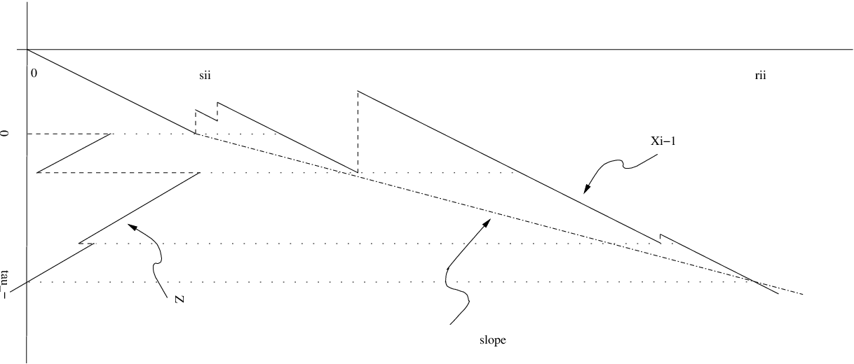
The idea is to apply Proposition A.1 to the process

Z⁡(x):=inf{t≥0:Xi−1​(σi(i))−Xi−1​(σi(i)+t)=x}−xci−1−ci,Z(x):=\inf\left\{t\geq 0:X_{i-1}\left(\sigma^{(i)}_{i}\right)-X_{i-1}\left(\sigma^{(i)}_{i}+t\right)=x\right\}-\frac{x}{c_{i-1}-c_{i}},

see Figure 1.

Refer to caption
Figure 1: Excursions of {Xi−1​(t)−X¯i−1​(t):t≥0}\{X_{i-1}(t)-\underline{X}_{i-1}(t):t\geq 0\} correspond to jumps of ZZ.

In this diagram, excursions of {Xi−1​(t)−X¯i−1​(t):t≥0}\{X_{i-1}(t)-\underline{X}_{i-1}(t):t\geq 0\} correspond to jumps of ZZ. The relevant information on the subexcursions is incorporated into ZZ as jump marks.

Observe that ZZ is a compound Poisson process with negative drift 1/ci−1−1/(ci−1−ci)1/c_{i-1}-1/(c_{i-1}-c_{i}) and intensity λ/ci−1\lambda/c_{i-1}, starting with a (marked) jump at zero. The jumps of ZZ correspond to (i−1)(i-1)-excursions, and the above marks are assigned to the each of the jumps. In terms of Proposition A.1, it remains to observe that ρi(i)−ρi−1(i)\rho^{(i)}_{i}-\rho^{(i)}_{i-1} and ρi(i)−σi(i)\rho^{(i)}_{i}-\sigma^{(i)}_{i} correspond to (τ−−TN−)/ci−1(\tau_{-}-T_{N_{-}})/c_{i-1} and τ−/(ci−1−ci)\tau_{-}/(c_{i-1}-c_{i}) respectively. □\Box

With the recursion of Lemma 4.1, we can find the joint transform of ρk(k)−ρj(k)\rho^{(k)}_{k}-\rho^{(k)}_{j} for j=1,…,k−1j=1,\ldots,k-1, which is required to work out Proposition 4.1. This is done in (14) below. It is equivalent to find the transform of ρj+1(k)−ρj(k)\rho^{(k)}_{j+1}-\rho^{(k)}_{j} for j=1,…,k−1j=1,\ldots,k-1, which is the content of the next proposition. We have also added ρk(k)−σk(k)\rho^{(k)}_{k}-\sigma^{(k)}_{k} for convenience. The resulting formula has some remarkable features similar to the formula in Theorem 3.1. Most interestingly, a quasi-product form appears here as well.

For β∈ℝ+k−1≥0\beta\in{\mathbb{R}}_{+}^{k-1}\geq 0, and j=1,…,k−1j=1,\ldots,k-1, we define

𝒞jk​(β):=cj​∑ℓ=jk−1(1cℓ+1−1cℓ)​(λ+βℓ).{\mathcal{C}}_{j}^{k}(\beta):=c_{j}\sum_{\ell=j}^{k-1}\left(\frac{1}{c_{\ell+1}}-\frac{1}{c_{\ell}}\right)(\lambda+\beta_{\ell}).
Proposition 4.2

Suppose that XX is an nn-dimensional Lévy process satisfying D and H. Then for any k=2,…,nk=2,\ldots,n, β∈ℝ+k−1\beta\in{\mathbb{R}}_{+}^{k-1}, γ≥0\gamma\geq 0, we have

𝔼e−∑j=1k−1βj(ρj+1(k)−ρ(k)j)−γ(ρk(k)−σk(k))\displaystyle{\mathbb{E}}{\rm e}^{{-\sum_{j=1}^{k-1}\beta_{j}\left(\rho_{j+1}^{(k)}-\rho^{(k)}_{j}\right)-\gamma\left(\rho_{k}^{(k)}-\sigma_{k}^{(k)}\right)}} =\displaystyle= ∏j=1k−1βj+λ​𝔼​e−[𝒞j+1k​(β)+cj+1ck​γ]​(ρj+1(j+1)−σj+1(j+1))βj+λ​𝔼​e−[𝒞jk​(β)+cjck​γ]​(ρj(j)−σj(j))\displaystyle\prod_{j=1}^{k-1}\frac{\beta_{j}+\lambda{\mathbb{E}}{\rm e}^{{-\left[{\mathcal{C}}_{j+1}^{k}(\beta)+\frac{c_{j+1}}{c_{k}}\gamma\right]\left(\rho_{j+1}^{(j+1)}-\sigma^{(j+1)}_{j+1}\right)}}}{\beta_{j}+\lambda{\mathbb{E}}{\rm e}^{{-\left[{\mathcal{C}}_{j}^{k}(\beta)+\frac{c_{j}}{c_{k}}\gamma\right]\left(\rho_{j}^{(j)}-\sigma^{(j)}_{j}\right)}}}
×𝔼​e−[𝒞1k​(β)+c1ck​γ]​(ρ1(1)−σ1(1)).\displaystyle\mbox{}\times{\mathbb{E}}{\rm e}^{{-\left[{\mathcal{C}}_{1}^{k}(\beta)+\frac{c_{1}}{c_{k}}\gamma\right]\left(\rho_{1}^{(1)}-\sigma^{(1)}_{1}\right)}}.

Proof. Since for ℓ=2,…,i\ell=2,\ldots,i, by definition of 𝒞ℓk​(β){\mathcal{C}}_{\ell}^{k}(\beta),

(cℓ−1cℓ−1)​(λ+βℓ−1)+cℓ−1cℓ​𝒞ℓk​(β)=𝒞ℓ−1k​(β),\left(\frac{c_{\ell-1}}{c_{\ell}}-1\right)(\lambda+\beta_{\ell-1})+\frac{c_{\ell-1}}{c_{\ell}}{\mathcal{C}}_{\ell}^{k}(\beta)={\mathcal{C}}_{\ell-1}^{k}(\beta),

it follows from Lemma 4.1 that

𝔼e−∑j=1ℓ−1βj(ρ(ℓ)j+1−ρ(ℓ)j)−[𝒞ℓk(β)+cℓckγ](ρ(ℓ)ℓ−σ(ℓ)ℓ)𝔼e−∑j=1ℓ−2βj(ρ(ℓ−1)j+1−ρ(ℓ−1)j)−[𝒞ℓ−1k(β)+cℓ−1ckγ](ρ(ℓ−1)ℓ−1−σ(ℓ−1)ℓ−1)\displaystyle\frac{{\mathbb{E}}{\rm e}^{{-\sum_{j=1}^{\ell-1}\beta_{j}\left(\rho^{(\ell)}_{j+1}-\rho^{(\ell)}_{j}\right)-\left[{\mathcal{C}}_{\ell}^{k}(\beta)+\frac{c_{\ell}}{c_{k}}\gamma\right]\left(\rho^{(\ell)}_{\ell}-\sigma^{(\ell)}_{\ell}\right)}}}{{\mathbb{E}}{\rm e}^{{-\sum_{j=1}^{\ell-2}\beta_{j}\left(\rho^{(\ell-1)}_{j+1}-\rho^{(\ell-1)}_{j}\right)-\left[{\mathcal{C}}_{\ell-1}^{k}(\beta)+\frac{c_{\ell-1}}{c_{k}}\gamma\right]\left(\rho^{(\ell-1)}_{\ell-1}-\sigma^{(\ell-1)}_{\ell-1}\right)}}} =\displaystyle= βℓ−1+λ​𝔼​e−𝒞ℓk​(β,γ)​(ρℓ(ℓ)−σℓ(ℓ))βℓ−1+λ​𝔼​e−𝒞ℓ−1k​(β,γ)​(ρℓ−1(ℓ−1)−σℓ−1(ℓ−1)).\displaystyle\frac{\beta_{\ell-1}+\lambda{\mathbb{E}}{\rm e}^{{-{\mathcal{C}}_{\ell}^{k}(\beta,\gamma)\left(\rho^{(\ell)}_{\ell}-\sigma^{(\ell)}_{\ell}\right)}}}{\beta_{\ell-1}+\lambda{\mathbb{E}}{\rm e}^{{-{\mathcal{C}}_{\ell-1}^{k}(\beta,\gamma)\left(\rho^{(\ell-1)}_{\ell-1}-\sigma^{(\ell-1)}_{\ell-1}\right)}}}.

The claim follows from this recursion (start with ℓ=k\ell=k and note that 𝒞kk​(β)=0{\mathcal{C}}^{k}_{k}(\beta)=0). □\Box

5 Multidimensional Skorokhod problems.

In the next sections, we apply results of the previous sections to the analysis of fluid networks. Such networks are closely related to (multidimensional) Skorokhod reflection problems, which we describe first. Subject to certain assumptions, we explicitly solve such a reflection problem in Section 5.1. Section 5.2 describes the fluid networks associated to these special Skorokhod problems.

Let PP be a nonnegative matrix with spectral radius strictly smaller than one. To a given càdlàg function YY with values in ℝn{\mathbb{R}}^{n} such that Y⁡(0)=0Y(0)=0, one can associate a càdlàg pair (W,L)(W,L) with the following properties (w∈ℝ+nw\in{\mathbb{R}}^{n}_{+}):

S1 W⁡(t)=w+Y⁡(t)+(I−P′)​L​(t),t≥0W(t)=w+Y(t)+(I-P^{\prime})L(t),t\geq 0,

S2 W⁡(t)≥0,t≥0W(t)\geq 0,t\geq 0 and W⁡(0)=wW(0)=w,

S3 L⁡(0)=0L(0)=0 and LL is nondecreasing, and

S4 ∑j=1n∫0∞Wj​(t)​d​Lj​(t)=0\sum_{j=1}^{n}\int_{0}^{\infty}W_{j}(t)\,dL_{j}(t)=0.

It is known that such a pair exists and that it is unique; see Harrison and Reiman [15] for the continuous case, Robert [35] or Whitt [37, Thm. 14.2.3] for the càdlàg case, and Kella [24] for a more general result.

It is said that (W,L)(W,L) is the solution to the Skorokhod problem of YY in ℝ+n{\mathbb{R}}^{n}_{+} with reflection matrix I−P′I-P^{\prime} and initial condition ww.

In general, the pair (W,L)(W,L) cannot be expressed explicitly in terms of the driving process YY, with the notable exception of the one-dimensional case. However, if the Skorokhod problem has a special structure, this property carries over to a multidimensional setting.

5.1 A special Skorokhod problem.

It is the aim of this subsection to solve the Skorokhod problem for the pair (W,L)(W,L) under the following assumptions:

N1 PP is strictly upper triangular,

N2 the jj-th column of PP contains exactly one strictly positive element for j=2,…,nj=2,\ldots,n, and

N3 YjY_{j} is nondecreasing for j=2,…,nj=2,\ldots,n.

In Section 5.2, we show that these assumptions impose a ‘tree’ structure on fluid networks.

Theorem 5.1

Under N1–N3, the solution to the Skorokhod problem of YY in ℝ+n{\mathbb{R}}_{+}^{n} is given by

L⁡(t)\displaystyle L(t) =\displaystyle= 0∨sup0≤s≤t[−(I−P′)−1​Y​(s)−(I−P′)−1​w],\displaystyle 0\vee\sup_{0\leq s\leq t}\left[-(I-P^{\prime})^{-1}Y(s)-(I-P^{\prime})^{-1}w\right],
W⁡(t)\displaystyle W(t) =\displaystyle= w+Y⁡(t)+(I−P′)​L​(t),\displaystyle w+Y(t)+(I-P^{\prime})L(t),

where the supremum should be interpreted componentwise.

Proof. As WW is determined by LL and S1, we only have to prove the expression for LL. By Theorem D.3 of Robert [35], we know that LiL_{i} satisfies the fixed-point equation

Li​(t)=0∨sup0≤s≤t[(P′​L)i​(s)−wi−Yi​(s)]L_{i}(t)=0\vee\sup_{0\leq s\leq t}\left[(P^{\prime}L)_{i}(s)-w_{i}-Y_{i}(s)\right] (5)

for i=1,…,ni=1,\ldots,n and t≥0t\geq 0.

As a consequence of N1, we have (I−P′)−1=I+P′+…+P′n−1(I-P^{\prime})^{-1}=I+P^{\prime}+\ldots+P^{\prime n-1}, and the jj-th row of (I−P′)−1(I-P^{\prime})^{-1} is the jj-th row of I+P′+P′2+…+P′j−1I+P^{\prime}+P^{\prime 2}+\ldots+P^{\prime j-1}. Therefore, the theorem asserts that

Li(t)=0∨sup0≤s≤t[−∑k=0i−1[P′kY(s)+P′kw)]i].L_{i}(t)=0\vee\sup_{0\leq s\leq t}\left[-\sum_{k=0}^{i-1}\left[P^{\prime k}Y(s)+P^{\prime k}w)\right]_{i}\right]. (6)

The proof goes by induction. For i=1i=1, (6) is the same equation as (5). Let us now suppose that we know that (6) holds for i=1,…,j−1i=1,\ldots,j-1, where j=2,…,nj=2,\ldots,n. Furthermore, let j∗<jj^{*}<j be such that pj∗​j>0p_{j^{*}j}>0; it is unique by N2. Equation (5) shows that

Lj​(t)\displaystyle L_{j}(t) =\displaystyle= 0∨sup0≤s≤t[pj∗​j​Lj∗​(s)−wj−Yj​(s)]\displaystyle 0\vee\sup_{0\leq s\leq t}\left[p_{j^{*}j}L_{j^{*}}(s)-w_{j}-Y_{j}(s)\right] (7)
=\displaystyle= 0∨sup0≤s≤t[(0∨sup0≤u≤s−∑k=0j∗−1pj∗​j[P′kY(u)+P′kw]j∗)−wj−Yj(s)]\displaystyle 0\vee\sup_{0\leq s\leq t}\left[\left(0\vee\sup_{0\leq u\leq s}-\sum_{k=0}^{j^{*}-1}p_{j^{*}j}\left[P^{\prime k}Y(u)+P^{\prime k}w\right]_{j^{*}}\right)-w_{j}-Y_{j}(s)\right]
=\displaystyle= 0∨sup0≤s≤t[sup0≤u≤s−∑k=0j∗−1pj∗​j[P′kY(u)+P′kw]j∗−wj−Yj(s)]\displaystyle 0\vee\sup_{0\leq s\leq t}\left[\sup_{0\leq u\leq s}-\sum_{k=0}^{j^{*}-1}p_{j^{*}j}\left[P^{\prime k}Y(u)+P^{\prime k}w\right]_{j^{*}}-w_{j}-Y_{j}(s)\right]
=\displaystyle= 0∨sup0≤u≤tsupu≤s≤t[−∑k=0j∗−1[P′k+1Y(u)+P′k+1w]j−wj−Yj(s)]\displaystyle 0\vee\sup_{0\leq u\leq t}\sup_{u\leq s\leq t}\left[-\sum_{k=0}^{j^{*}-1}\left[P^{\prime k+1}Y(u)+P^{\prime k+1}w\right]_{j}-w_{j}-Y_{j}(s)\right]
=\displaystyle= 0∨sup0≤u≤t[−∑k=0j∗[P′kY(u)+P′kw]j],\displaystyle 0\vee\sup_{0\leq u\leq t}\left[-\sum_{k=0}^{j^{*}}\left[P^{\prime k}Y(u)+P^{\prime k}w\right]_{j}\right], (8)

where we have used N3 for the equalities (7) and (8).

The proof is completed after noting that the jj-th row of P′kP^{\prime k} only contains zeroes for k=j∗+1,…,j−1k=j^{*}+1,\ldots,j-1. □\Box

Instead of working directly with WW, it is often convenient to work with a transformed version, W~:=(I−P′)−1​W\widetilde{W}:=(I-P^{\prime})^{-1}W. The process W~\widetilde{W} lies in a cone 𝒞{\cal C}, which is a polyhedron and a proper subset of the orthant ℝ+n{\mathbb{R}}^{n}_{+}. Under the present assumptions, at least one edge of 𝒞{\cal C} is in the interior of ℝ+n{\mathbb{R}}_{+}^{n} and at least one is an axis. Below we give an interpretation of W~\widetilde{W}.

We next establish a correspondence between the event that Wj​(t)=0W_{j}(t)=0 and W~j​(t)=0\widetilde{W}_{j}(t)=0 under an additional condition.

Proposition 5.1

Suppose that N1–N3 hold, but with ‘nondecreasing’ replaced by ‘strictly increasing’ in N3. Then we have Wj​(t)=0W_{j}(t)=0 if and only if W~j​(t)=0\widetilde{W}_{j}(t)=0, for any j=1,…,nj=1,\ldots,n and t≥0t\geq 0.

Proof. For j=1j=1 we have Wj​(t)=W~j​(t)W_{j}(t)=\widetilde{W}_{j}(t), so the stated is satisfied; suppose therefore that j>1j>1. Since the matrix (I−P′)−1(I-P^{\prime})^{-1} is lower triangular and nonnegative, we straightforwardly get that W~j​(t)=0\widetilde{W}_{j}(t)=0 implies Wj​(t)=0{W}_{j}(t)=0.

For the converse, observe that under N1–N2 (see the proof of Theorem 5.1; we use the same notation)

W~j​(t)=∑k=0j−1[P′k​W]j​(t)=∑k=0j∗[P′k​W]j​(t).\widetilde{W}_{j}(t)=\sum_{k=0}^{j-1}\left[P^{\prime k}W\right]_{j}(t)=\sum_{k=0}^{j^{*}}\left[P^{\prime k}W\right]_{j}(t).

An induction argument shows that it suffices to prove that Wj​(t)=0W_{j}(t)=0 implies Wj∗​(t)=0W_{j^{*}}(t)=0. To see that this holds, we observe that by S1 and (5), Wj​(t)=0W_{j}(t)=0 is equivalent to

pj∗​j​Lj∗​(t)−wj−Yj​(t)=0∨sup0≤s≤t[pj∗​j​Lj∗​(s)−wj−Yj​(s)].p_{j^{*}j}L_{j^{*}}(t)-w_{j}-Y_{j}(t)=0\vee\sup_{0\leq s\leq t}\left[p_{j^{*}j}L_{j^{*}}(s)-w_{j}-Y_{j}(s)\right].

The right-hand side of this equality is clearly nondecreasing. Therefore, since YjY_{j} is strictly increasing by assumption, we conclude that d​Lj∗​(t)>0dL_{j^{*}}(t)>0, which immediately yields Wj∗​(t)=0W_{j^{*}}(t)=0 by S4. This completes the proof. □\Box

5.2 Lévy-driven tree fluid networks.

In this subsection, we define a class of Lévy-driven fluid networks, which we call tree fluid networks. We are interested in the steady-state behavior of such networks.

Consider nn (infinite-buffer) fluid queues, with external input to queue jj in the time interval [0,t][0,t] given by Jj​(t)J_{j}(t). We assume that J={J(t):t≥0}={(J1(t),…,Jn(t))′:t≥0}J=\{J(t):t\geq 0\}=\{(J_{1}(t),\ldots,J_{n}(t))^{{}^{\prime}}:t\geq 0\} is a càdlàg Lévy process starting in J⁡(0)=0∈ℝ+nJ(0)=0\in{\mathbb{R}}^{n}_{+}. The buffers are continuously drained at a constant rate as long as there is content in the buffer. These drain rates are given by a vector rr; for buffer jj, the rate is rj>0r_{j}>0.

The interaction between the queues is modeled as follows. A fraction pi​jp_{ij} of the output of station ii is immediately transferred to station jj, while a fraction 1−∑j≠ipi​j1-\sum_{j\neq i}p_{ij} leaves the system. We set pi​i=0p_{ii}=0 for all ii, and suppose that ∑jpi​j≤1\sum_{j}p_{ij}\leq 1. The matrix P={pi​j:i,j=1,…,n}P=\{p_{ij}:i,j=1,\ldots,n\} is called the routing matrix. We assume that for any station ii, there is at most one station feeding buffer ii, and that pi​j=0p_{ij}=0 for j<ij<i. The resulting network can be represented by a (directed) tree. Indeed, the stations then correspond to nodes, and there is a vertex from station ii and jj if pi​j>0p_{ij}>0. This motivates the name ‘tree fluid networks’. We represent such a fluid network by the triplet (J,r,P)(J,r,P). Note that PP satisfies N1–N2 by definition of a tree fluid network.

The buffer content process WW and regulator LL associated to the fluid network (J,r,P)(J,r,P) are defined as the solution of the Skorokhod problem of

Y⁡(t):=J⁡(t)−(I−P′)​r​tY(t):=J(t)-(I-P^{\prime})rt

with reflection matrix I−P′I-P^{\prime}. The buffer content is sometimes called the workload, explaining the notation WW. Importantly, the dynamics of the network are given by S1–S4, as the reader may verify. The process LjL_{j} can be interpreted as the cumulative unused capacity in station jj.

Associated to the processes WW and LL, one can also define the process of the age of the busy period: for j=1,…,nj=1,\ldots,n, we set

Bj​(t):=t−sup{s≤t:Wj​(s)=0},B_{j}(t):=t-\sup\{s\leq t:W_{j}(s)=0\}, (9)

and let B⁡(t)=(B1​(t),…,Bn​(t))′B(t)=(B_{1}(t),\ldots,B_{n}(t))^{\prime}. Hence, if there is work in queue jj at time tt (that is, Wj​(t)>0W_{j}(t)>0), Bj​(t)B_{j}(t) is the time that elapsed after the last time that the jj-th queue was empty. If there is no work in queue ii at time tt, then Bi​(t)=0B_{i}(t)=0. Similarly, one can also define the age of the idle period for j=1,…,nj=1,\ldots,n:

Ij​(t):=t−sup{s≤t:Wj​(s)≠0},I_{j}(t):=t-\sup\{s\leq t:W_{j}(s)\neq 0\},

and the corresponding vector I⁡(t)I(t). As a result of these definitions, Ij​(t)>0I_{j}(t)>0 implies Bj​(t)=0B_{j}(t)=0 and Bj​(t)>0B_{j}(t)>0 implies Ij​(t)=0I_{j}(t)=0 for j=1,…,nj=1,\ldots,n. The quantities B~j​(t)\widetilde{B}_{j}(t) and I~j​(t)\widetilde{I}_{j}(t) are defined similarly, but with WjW_{j} replaced by the jj-th element of W~=(I−P′)−1​W\widetilde{W}=(I-P^{\prime})^{-1}W.

The random variables W~j\widetilde{W}_{j}, B~j\widetilde{B}_{j}, and I~j\widetilde{I}_{j} have a natural interpretation. Indeed, let us consider all stations on a path from the root of the tree to station jj. The total content of the buffers along this path is then given by W~j\widetilde{W}_{j}. Consequently, B~j\widetilde{B}_{j} and I~j\widetilde{I}_{j} correspond to the ages of the busy and idle periods of this aggregate buffer.

In the rest of the paper, we assume that the tree fluid network has the following additional properties:

T1

If pi​j>0p_{ij}>0, then pi​j>rj/rip_{ij}>r_{j}/r_{i},

T2

Jj​(t)J_{j}(t) are nondecreasing for j=2,…,nj=2,\ldots,n,

T3

JJ is an nn-dimensional Lévy process, and

T4

JJ is integrable and (I−P′)−1​𝔼​J​(1)<r(I-P^{\prime})^{-1}{\mathbb{E}}J(1)<r.

An important consequence of T1 and T2 is that YY is componentwise nondecreasing, except for Y1Y_{1}. Consequently, if T1 and T2 hold for a tree fluid network, then N1–N3 are automatically satisfied for the associated Skorokhod problem. Hence, Theorem 5.1 gives an explicit description of the buffer contents in the network. Note that T4 ensures stability of the network.

Let us now define the process

X⁡(t):=(I−P′)−1​Y​(t)=(I−P′)−1​J​(t)−r​t.X(t):=(I-P^{\prime})^{-1}Y(t)=(I-P^{\prime})^{-1}J(t)-rt.

In view of assumption T1, the down-stream buffer contents always grow when one of the up-stream buffers is nonempty. Moreover, under T1, W~\widetilde{W} is itself a reflected process, that is (W~,L~)(\widetilde{W},\widetilde{L}) is the solution to the Skorokhod problem for XX with reflection matrix II and initial condition (I−P′)−1​w(I-P^{\prime})^{-1}w. Therefore, each coordinate of W~\tilde{W} is a one-dimensional reflected process. A similar assumption facilitates the analysis in [20], [22, Thm. 4.1 and Lem. 4.2], and [25].

In the next proposition, we find the steady-state behavior of the buffer content and the age of the busy (and idle) period for the Lévy-driven tree fluid network (J,r,P)(J,r,P). We also consider the case where the inequality pi​j>rj/rip_{ij}>r_{j}/r_{i} in T1 holds only weakly (i.e. pi​j≥rj/rip_{ij}\geq r_{j}/r_{i}), as this plays a role in priority fluid systems (see Section 6.3 below).

Recall the definitions of G=GXG=G^{X} and H=HXH=H^{X} in Sections 2.1 and 2.2 respectively.

Proposition 5.2

Suppose that T1–T4 hold for the tree fluid network (J,r,P)(J,r,P).

  • (i)

    For any initial condition W⁡(0)=wW(0)=w, the triplet of vectors (W⁡(t),B⁡(t),I⁡(t))(W(t),B(t),I(t)) converges in distribution to ((I−P′)​X¯,GX,HX)((I-P^{\prime})\overline{X},G^{X},H^{X}) as t→∞t\to\infty.

  • (ii)

    If the second inequality in T1 holds only weakly, then for any initial condition W⁡(0)=wW(0)=w, the triplet of vectors (W​(t),B~​(t),I~​(t))(W(t),\widetilde{B}(t),\widetilde{I}(t)) converges in distribution to ((I−P′)​X¯,GX,HX)((I-P^{\prime})\overline{X},G^{X},H^{X}) as t→∞t\to\infty.

Proof. Throughout this proof, a system of equations like (9) is abbreviated by B⁡(t)=t−sup{s≤t:W⁡(s)=0}B(t)=t-\sup\{s\leq t:W(s)=0\}.

We start with the proof of (ii). By Theorem 5.1, we have for any t>0t>0

W~​(t)=[x+X⁡(t)]∨sup0≤s≤t[X⁡(t)−X⁡(s)],\widetilde{W}(t)=[x+X(t)]\vee\sup_{0\leq s\leq t}[X(t)-X(s)],

where x=(I−P′)−1​wx=(I-P^{\prime})^{-1}w. Moreover, as a consequence of Proposition 5.1, we have

B~​(t)\displaystyle\widetilde{B}(t) =\displaystyle= t−sup{s≤t:W~​(s)=0}\displaystyle t-\sup\{s\leq t:\widetilde{W}(s)=0\}
=\displaystyle= t−sup{s≤t:x+X⁡(s)=0∧inf0≤u≤s[x+X⁡(u)]}\displaystyle t-\sup\left\{s\leq t:x+X(s)=0\wedge\inf_{0\leq u\leq s}[x+X(u)]\right\}
=\displaystyle= t−sup{s≤t:x+X⁡(s)=0∧inf0≤u≤t[x+X⁡(u)]},\displaystyle t-\sup\left\{s\leq t:x+X(s)=0\wedge\inf_{0\leq u\leq t}[x+X(u)]\right\},

where the last equality is best understood by sketching a sample path of XX. The supremum over an empty set should be interpreted as zero.

This reasoning carries over to idle periods:

I~​(t)=t−sup{s≤t:x+X⁡(s)≠0∧inf0≤u≤s[x+X⁡(u)]}.\widetilde{I}(t)=t-\sup\left\{s\leq t:x+X(s)\neq 0\wedge\inf_{0\leq u\leq s}[x+X(u)]\right\}.

Due to the stationarity of the increments of {X⁡(t),t≥0}\{X(t),\ t\geq 0\} (T3), we may extend XX to the two-sided process {X⁡(t),t∈ℝ}\{X(t),\ t\in{\mathbb{R}}\}. This leads to

(W~​(t)B~​(t)I~​(t))=d([x−X⁡(−t)]∨sup−t≤s≤0[−X⁡(s)]−sup{s:−t≤s≤0,−X(s)=[x−X(−t)]∨sup−t≤u≤0[−X(u)]}−sup{s:−t≤s≤0,−X(s)≠[x−X(−t)]∨sup−t≤u≤s[−X(u)]}).\left(\begin{array}[]{c}\widetilde{W}(t)\\ \widetilde{B}(t)\\ \widetilde{I}(t)\end{array}\right)=_{\rm d}\left(\begin{array}[]{c}[x-X(-t)]\vee\sup_{-t\leq s\leq 0}[-X(s)]\\ -\sup\left\{s:-t\leq s\leq 0,-X(s)=[x-X(-t)]\vee\sup_{-t\leq u\leq 0}[-X(u)]\right\}\\ -\sup\left\{s:-t\leq s\leq 0,-X(s)\neq[x-X(-t)]\vee\sup_{-t\leq u\leq s}[-X(u)]\right\}\end{array}\right).

Since x−X⁡(−t)→−∞x-X(-t)\to-\infty almost surely by T4, this tends to

(sups≤0[−X⁡(s)]−sup{s≤0:−X(s)=supu≤0[−X(u)]}−sup{s≤0:−X(s)≠supu≤s[−X(u)]}),\left(\begin{array}[]{c}\sup_{s\leq 0}[-X(s)]\\ -\sup\left\{s\leq 0:-X(s)=\sup_{u\leq 0}[-X(u)]\right\}\\ -\sup\left\{s\leq 0:-X(s)\neq\sup_{u\leq s}[-X(u)]\right\}\end{array}\right),

a vector that is almost surely finite, again by T4. By time-reversibility (see Lemma II.2 of Bertoin [4]), the latter vector is equal in distribution to (X¯,GX,HX)(\overline{X},G^{X},H^{X}).

The first claim follows from (ii) after noting that B​(t)=B~​(t)B(t)=\widetilde{B}(t) and I​(t)=I~​(t)I(t)=\widetilde{I}(t) by Proposition 5.1. □\Box

We remark that the above proof does not use T3 to the fullest. Indeed, for the proposition to hold, it suffices that JJ has stationary increments and that it is time-reversible.

Let us now suppose that the initial buffer content ww is random. Proposition 5.2 shows, after a standard argument, that {W⁡(t)}\{W(t)\} is a stationary process if W⁡(0)=wW(0)=w is distributed as μ∗\mu^{*}, where μ∗\mu^{*} is the distribution of (I−P′)​X¯(I-P^{\prime})\overline{X}. We now show that this stationary distribution is unique.

Corollary 5.1

Suppose that T1–T4 hold for the tree fluid network (J,r,P)(J,r,P). Then μ∗\mu^{*} is the only stationary distribution.

Proof. Suppose there exists another stationary distribution μ0∗≠μ∗\mu^{*}_{0}\neq\mu^{*}. Let W0∗W^{*}_{0} be the corresponding stationary process. For any Borel set BB in ℝ+n{\mathbb{R}}_{+}^{n} and any t≥0t\geq 0, we then have ℙ⁡(W0∗​(0)∈B)=ℙ⁡(W0∗​(t)∈B)\mathbb{P}(W^{*}_{0}(0)\in B)=\mathbb{P}(W^{*}_{0}(t)\in B). Therefore,

ℙ⁡(W0∗​(0)∈B)\displaystyle\mathbb{P}(W^{*}_{0}(0)\in B) =\displaystyle= limt→∞ℙ⁡(W0∗​(t)∈B)\displaystyle\lim_{t\to\infty}\mathbb{P}(W^{*}_{0}(t)\in B)
=\displaystyle= limt→∞∫0∞ℙ⁡(W0∗​(t)∈B|W0∗​(0)=w)​ℙ​(W0∗​(0)∈𝑑w)\displaystyle\lim_{t\to\infty}\int_{0}^{\infty}\mathbb{P}(W^{*}_{0}(t)\in B|W^{*}_{0}(0)=w)\mathbb{P}(W^{*}_{0}(0)\in dw)
=\displaystyle= ∫0∞limt→∞ℙ⁡(W0∗​(t)∈B|W0∗​(0)=w)​ℙ​(W0∗​(0)∈𝑑w)\displaystyle\int_{0}^{\infty}\lim_{t\to\infty}\mathbb{P}(W^{*}_{0}(t)\in B|W^{*}_{0}(0)=w)\mathbb{P}(W^{*}_{0}(0)\in dw)
=\displaystyle= ∫0∞ℙ⁡((I−P′)​X¯∈B)​ℙ​(W0∗​(0)∈𝑑w)=ℙ⁡((I−P′)​X¯∈B),\displaystyle\int_{0}^{\infty}\mathbb{P}((I-P^{\prime})\overline{X}\in B)\mathbb{P}(W^{*}_{0}(0)\in dw)=\mathbb{P}((I-P^{\prime})\overline{X}\in B),

where the second last equation is due to Proposition 5.2. This is clearly a contradiction. □\Box

Corollary 5.1 answers, for the special case of tree fluid networks, a question from the paper of Konstantopolous, Last and Lin [28] on the uniqueness of the stationary distribution. Note that for the queueing problem related to (J,r,P)(J,r,P), the uniqueness of the stationary distribution was discussed in Kella [22]. In contrast to the setting in [22], we allow for the first component of J⁡(t)J(t) to be a general Lévy process.

In the next section, we combine Proposition 5.2 with the results given in Sections 3 and 4 to study particular networks.

6 Tandem networks and priority systems.

In this section, we analyze nn fluid queues in tandem, which is a tree fluid network with a special structure. We also analyze a closely related priority system.

The tandem structure is specified by the form of the routing matrix: we suppose that PP is such that pi,i+1>0p_{i,i+1}>0 for i=1,…,n−1i=1,\ldots,n-1, and pi​j=0p_{ij}=0 otherwise. Observe that we allow pi,i+1>1p_{i,i+1}>1, and that it is not really a restriction to exclude pi,i+1=0p_{i,i+1}=0; otherwise the queueing system splits into independent tandem networks.

In all of our results, we suppose that the tandem system (J,r,P)(J,r,P) satisfies T1–T4. We rule out the degenerate case where the first j≥1j\geq 1 components of JJ are deterministic drifts, since an equivalent problem can then be studied with the first jj stations removed. We also impose the following assumptions on the input Lévy process JJ:

T5 JJ has mutually independent components, and

T6 The Lévy measure of J1J_{1} is supported on ℝ+{\mathbb{R}}_{+}.

Observe that under T2–T3, T5 implies that J2,…,JnJ_{2},\ldots,J_{n} are independent nonnegative subordinators.

This section consists of three parts. In Section 6.1, we are interested in the joint (steady-state) distribution of the buffer contents and the ages of the busy periods for fluid tandem networks, i.e., in the distribution of (W⁡(∞),B⁡(∞))(W(\infty),B(\infty)). Section 6.2 considers the situation of a single compound Poisson input to the system. For that system, we are also interested in the ages of the idle periods, i.e., in the vector I⁡(∞)I(\infty). In Section 6.3, we analyze buffer contents and busy periods in a priority system.

6.1 Generalities.

To find the joint distribution of W⁡(∞)W(\infty) and B⁡(∞)B(\infty), throughout this section denoted by WW and BB respectively, we rely on Proposition 5.2. This motivates the analysis of X⁡(t)=(I−P′)−1​J​(t)−r​tX(t)=(I-P^{\prime})^{-1}J(t)-rt. For i=2,…,ni=2,\ldots,n, we define the cumulant of Ji​(t)J_{i}(t) by θiJ​(β):=−log⁡𝔼​e−β​Ji​(1)\theta_{i}^{J}(\beta):=-\log{\mathbb{E}}{\rm e}^{{-\beta J_{i}(1)}}, β≥0\beta\geq 0. As in Section 4, we write ψi\psi_{i} (defined by ψi​(β)=log⁡𝔼​e−β​Xi​(1)\psi_{i}(\beta)=\log{\mathbb{E}}{\rm e}^{{-\beta X_{i}(1)}}) for the Laplace exponent of −Xi-X_{i}. Its inverse is again denoted by Φi\Phi_{i}.

Under T2 and T6, the Lévy measure of XX is supported on ℝ+n{\mathbb{R}}_{+}^{n}. Moreover, as we ruled out trivial queues in the network, each of the components of X¯\overline{X} has a nondegenerate distribution. Therefore, let us recall that the following holds (see, e.g., Theorem VII.4 in [4]): for α,β≥0\alpha,\beta\geq 0, (α,β)≠(0,0)(\alpha,\beta)\neq(0,0), β≠Φi​(α)\beta\neq\Phi_{i}(\alpha), i=1,…,ni=1,\ldots,n, we have

𝔼​e−α​Gi−β​X¯i=−𝔼​Xi​(1)​Φi​(α)−βα−ψi​(β).{\mathbb{E}}{\rm e}^{{-\alpha G_{i}-\beta\overline{X}_{i}}}=-{\mathbb{E}}X_{i}(1)\frac{\Phi_{i}\left(\alpha\right)-\beta}{\alpha-\psi_{i}(\beta)}. (10)

This identity plays a crucial role in the results of this section. For notational convenience, we shall write that (10) holds for any α,β≥0\alpha,\beta\geq 0, without the requirements (α,β)≠(0,0)(\alpha,\beta)\neq(0,0) and β≠Φi​(α)\beta\neq\Phi_{i}(\alpha).

Now we can formulate the main result of this subsection. We remark that the first formula also holds if J1J_{1} is not necessarily spectrally positive. For instance, it allows for phase-type downward jumps; see [7] for the joint transform of X¯j{\overline{X}}_{j} and GjG_{j} in that case.

Theorem 6.1

Consider a tandem fluid network (J,r,P)(J,r,P) for which T1–T6 holds. Then for ω,β∈ℝ+n\omega,\beta\in{\mathbb{R}}_{+}^{n}, the transform 𝔼​e−⟨ω,W⟩−⟨β,B⟩{\mathbb{E}}{\rm e}^{{-\langle\omega,W\rangle-\langle\beta,B\rangle}} equals

∏j=1n−1𝔼​e−[∑ℓ=j+1nθℓJ​(ωℓ)+∑ℓ=j+1n(pℓ−1​ℓ​rℓ−1−rℓ)​ωℓ+∑ℓ=jnβℓ]​Gj−ωj​X¯j𝔼​e−[∑ℓ=j+1nθℓJ​(ωℓ)+∑ℓ=j+1n(pℓ−1​ℓ​rℓ−1−rℓ)​ωℓ+∑ℓ=j+1nβℓ]​Gj−pj,j+1​ωj+1​X¯j×𝔼​e−βn​Gn−ωn​X¯n.\prod_{j=1}^{n-1}\frac{{\mathbb{E}}{\rm e}^{{-\left[\sum_{\ell=j+1}^{n}\theta^{J}_{\ell}\left(\omega_{\ell}\right)+\sum_{\ell=j+1}^{n}(p_{\ell-1\ell}r_{\ell-1}-r_{\ell})\omega_{\ell}+\sum_{\ell=j}^{n}\beta_{\ell}\right]G_{j}-\omega_{j}\overline{X}_{j}}}}{{\mathbb{E}}{\rm e}^{{-\left[\sum_{\ell=j+1}^{n}\theta^{J}_{\ell}\left(\omega_{\ell}\right)+\sum_{\ell=j+1}^{n}(p_{\ell-1\ell}r_{\ell-1}-r_{\ell})\omega_{\ell}+\sum_{\ell=j+1}^{n}\beta_{\ell}\right]G_{j}-p_{j,j+1}\omega_{j+1}\overline{X}_{j}}}}\times{\mathbb{E}}{\rm e}^{{-\beta_{n}G_{n}-\omega_{n}\overline{X}_{n}}}.

Consequently, we have for ω,β∈ℝ+n\omega,\beta\in{\mathbb{R}}_{+}^{n},

𝔼​e−⟨ω,W⟩−⟨β,B⟩=−𝔼​Xn​(1)​Φn​(βn)−ωnβn−ψn​(ωn)\displaystyle{\mathbb{E}}{\rm e}^{{-\langle\omega,W\rangle-\langle\beta,B\rangle}}=-{\mathbb{E}}X_{n}(1)\frac{\Phi_{n}\left(\beta_{n}\right)-\omega_{n}}{\beta_{n}-\psi_{n}(\omega_{n})}
×\displaystyle\times ∏j=1n−1Φj​(∑ℓ=j+1nθℓJ​(ωℓ)+∑ℓ=j+1n(pℓ−1,ℓ​rℓ−1−rℓ)​ωℓ+∑ℓ=jnβℓ)−ωjΦj​(∑ℓ=j+1nθℓJ​(ωℓ)+∑ℓ=j+1n(pℓ−1,ℓ​rℓ−1−rℓ)​ωℓ+∑ℓ=j+1nβℓ)−pj,j+1​ωj+1\displaystyle\prod_{j=1}^{n-1}\frac{\Phi_{j}\left(\sum_{\ell=j+1}^{n}\theta^{J}_{\ell}\left(\omega_{\ell}\right)+\sum_{\ell=j+1}^{n}(p_{\ell-1,\ell}r_{\ell-1}-r_{\ell})\omega_{\ell}+\sum_{\ell=j}^{n}\beta_{\ell}\right)-\omega_{j}}{\Phi_{j}\left(\sum_{\ell=j+1}^{n}\theta^{J}_{\ell}\left(\omega_{\ell}\right)+\sum_{\ell=j+1}^{n}(p_{\ell-1,\ell}r_{\ell-1}-r_{\ell})\omega_{\ell}+\sum_{\ell=j+1}^{n}\beta_{\ell}\right)-p_{j,j+1}\omega_{j+1}}
×\displaystyle\times ∏j=1n−1∑ℓ=j+1nθℓJ​(ωℓ)+∑ℓ=j+1n(pℓ−1,ℓ​rℓ−1−rℓ)​ωℓ+∑ℓ=j+1nβℓ−ψj​(pj,j+1​ωj+1)∑ℓ=j+1nθℓJ​(ωℓ)+∑ℓ=j+1n(pℓ−1,ℓ​rℓ−1−rℓ)​ωℓ+∑ℓ=jnβℓ−ψj​(ωj).\displaystyle\prod_{j=1}^{n-1}\frac{\sum_{\ell=j+1}^{n}\theta^{J}_{\ell}\left(\omega_{\ell}\right)+\sum_{\ell=j+1}^{n}(p_{\ell-1,\ell}r_{\ell-1}-r_{\ell})\omega_{\ell}+\sum_{\ell=j+1}^{n}\beta_{\ell}-\psi_{j}(p_{j,j+1}\omega_{j+1})}{\sum_{\ell=j+1}^{n}\theta^{J}_{\ell}\left(\omega_{\ell}\right)+\sum_{\ell=j+1}^{n}(p_{\ell-1,\ell}r_{\ell-1}-r_{\ell})\omega_{\ell}+\sum_{\ell=j}^{n}\beta_{\ell}-\psi_{j}(\omega_{j})}.

Proof. By Proposition 5.2(i), (W,B)=d((I−P′)X¯,GX)(W,B)=_{\rm d}((I-P^{\prime})\overline{X},G^{X}). Hence we have

𝔼​e−⟨ω,W⟩−⟨β,B⟩=𝔼​e−⟨(I−P)​ω,(I−P′)−1​W⟩−⟨β,B⟩=𝔼​e−⟨β,G⟩−⟨(I−P)​ω,X¯⟩.{\mathbb{E}}{\rm e}^{{-\langle\omega,W\rangle-\langle\beta,B\rangle}}={\mathbb{E}}{\rm e}^{{-\langle(I-P)\omega,(I-P^{\prime})^{-1}W\rangle-\langle\beta,B\rangle}}={\mathbb{E}}{\rm e}^{{-\langle\beta,G\rangle-\langle(I-P)\omega,\overline{X}\rangle}}. (11)

Now note that the stability condition T4 for (J,r,P)(J,r,P) implies D for XX by the law of large numbers. Thus, in order to apply Theorem 3.1 for (11), it is enough to check that G holds. Standard algebraic manipulations give

X1​(t)=J1​(t)−r1​tX_{1}(t)=J_{1}(t)-r_{1}t

and

Xi+1​(t)=pi,i+1​Xi​(t)+Ji+1​(t)+(pi,i+1​ri−ri+1)​tX_{i+1}(t)=p_{i,i+1}X_{i}(t)+J_{i+1}(t)+(p_{i,i+1}r_{i}-r_{i+1})t

for i=1,…,n−1i=1,\ldots,n-1. Hence, G holds with Ki=pi−1,iK_{i}=p_{i-1,i} and Υi​(t)=Ji​(t)+(pi−1,i​ri−1−ri)​t\Upsilon_{i}(t)=J_{i}(t)+(p_{i-1,i}r_{i-1}-r_{i})t.

As a result, we know that from Theorem 3.1,

𝔼​e−⟨β,G⟩−⟨(I−P)​ω,X¯⟩=𝔼​e−⟨β,G⟩−⟨ω~,X¯⟩\displaystyle{\mathbb{E}}{\rm e}^{{-\langle\beta,G\rangle-\langle(I-P)\omega,\overline{X}\rangle}}={\mathbb{E}}{\rm e}^{{-\langle\beta,G\rangle-\langle\widetilde{\omega},\overline{X}\rangle}}
=\displaystyle= ∏j=1n−1𝔼​e−[∑ℓ=j+1nθℓΥ​(∑k=ℓnKℓk​ω~k)+∑ℓ=jnβℓ]​Gj−(∑k=jnKjk​ω~k)​X¯j𝔼​e−[∑ℓ=j+1nθℓΥ​(∑k=ℓnKℓk​ω~k)+∑ℓ=j+1nβℓ]​Gj−(∑k=j+1nKjk​ω~k)​X¯j×𝔼​e−βn​Gn−ω~n​X¯n,\displaystyle\prod_{j=1}^{n-1}\frac{{\mathbb{E}}{\rm e}^{{-\left[\sum_{\ell=j+1}^{n}\theta^{\Upsilon}_{\ell}\left(\sum_{k=\ell}^{n}K_{\ell}^{k}\widetilde{\omega}_{k}\right)+\sum_{\ell=j}^{n}\beta_{\ell}\right]G_{j}-\left(\sum_{k=j}^{n}K_{j}^{k}\widetilde{\omega}_{k}\right)\overline{X}_{j}}}}{{\mathbb{E}}{\rm e}^{{-\left[\sum_{\ell=j+1}^{n}\theta^{\Upsilon}_{\ell}\left(\sum_{k=\ell}^{n}K_{\ell}^{k}\widetilde{\omega}_{k}\right)+\sum_{\ell=j+1}^{n}\beta_{\ell}\right]G_{j}-\left(\sum_{k=j+1}^{n}K_{j}^{k}\widetilde{\omega}_{k}\right)\overline{X}_{j}}}}\times{\mathbb{E}}{\rm e}^{{-\beta_{n}G_{n}-\widetilde{\omega}_{n}\overline{X}_{n}}},

where we have set ω~=(I−P)​ω\widetilde{\omega}=(I-P)\omega for notational convenience.

The reader may check that ∑k=jnKjk​ω~k=ωj\sum_{k=j}^{n}K_{j}^{k}\widetilde{\omega}_{k}=\omega_{j} and ∑k=j+1nKjk​ω~k=pj,j+1​ωj+1\sum_{k=j+1}^{n}K_{j}^{k}\widetilde{\omega}_{k}=p_{j,j+1}\omega_{j+1}, leading to the first claim. The second assertion is a consequence of the first and (10). □\Box

Theorem 6.1 extends several results from the literature on the steady-state distribution of the buffer content for tandem Lévy networks. In particular, if J⁡(t)=(J1​(t),0)′J(t)=(J_{1}(t),0)^{\prime}, P=(pi​j)P=(p_{ij}), with p12=1p_{12}=1 and zeroes elsewhere, if one chooses β1=β2=0\beta_{1}=\beta_{2}=0 and ω1=0\omega_{1}=0 in Theorem 6.1, then one obtains Theorem 3.2 of Dȩbicki, Mandjes and van Uitert [6]. Additionally, if one chooses β1=β2=0\beta_{1}=\beta_{2}=0 and supposes that J1J_{1} is a subordinator, we recover the results of Kella [20].

Even if the Laplace transform of (Gj,X¯j)(G_{j},\overline{X}_{j}) can be inverted, it is generally not straightforward to invert the Laplace transform of (W,B)(W,B) given in Theorem 6.1. Some progress has been recently made in case n=2n=2; for a Brownian fluid system, Lieshout and Mandjes [30] calculate the distribution of WW. Avram, Palmowski, and Pistorius [2] study a compound Poisson setting with exponential jumps. A different type of explicit solution can be found in the work of Harrison [14]; he gives an example closely related to the framework of the present paper.

For use in Section 6.3, we point out that the expression in Theorem 6.1 is 𝔼​e−⟨ω,W⟩−⟨β,B~⟩{\mathbb{E}}{\rm e}^{{-\langle\omega,W\rangle-\langle\beta,\widetilde{B}\rangle}} if the second inequality in T1 is weak, cf. Proposition 5.2(ii).

The lengths of the busy periods.

Besides the Laplace transforms of the ages BB of the busy periods, Theorem 6.1 also enables us to find the Laplace transforms of the length VV of the steady-state running busy periods. Indeed, let DiD_{i}, i=1,…,ni=1,\ldots,n denote the steady-state remaining lengths of the running busy period, so that Vi=Bi+DiV_{i}=B_{i}+D_{i}. We know that DiD_{i} and BiB_{i} are equal in distribution. In fact, following for instance [1, Sec. V.3], we have

(Bi,Di)=d(UiVi,(1−Ui)Vi),\displaystyle(B_{i},D_{i})=_{\rm d}(U_{i}V_{i},(1-U_{i})V_{i}), (12)

where UiU_{i} are i.i.d. and uniform on [0,1][0,1].

For the Brownian (single-station) fluid queue, the following result is Corollary 3.8 of Salminen and Norros [36].

Corollary 6.1

Consider a tandem fluid network (J,r,P)(J,r,P) for which T1–T6 holds. Then for α,β≥0\alpha,\beta\geq 0, α≠β\alpha\neq\beta,

𝔼​e−α​Bi−β​Di=−𝔼​Xi​(1)​Φi​(α)−Φi​(β)α−β.{\mathbb{E}}{\rm e}^{{-\alpha B_{i}-\beta D_{i}}}=-{\mathbb{E}}X_{i}(1)\frac{\Phi_{i}(\alpha)-\Phi_{i}(\beta)}{\alpha-\beta}.

Moreover, we have for α≥0\alpha\geq 0,

𝔼​e−α​Vi=−𝔼​Xi​(1)​d​Φi​(α)d​α.{\mathbb{E}}{\rm e}^{{-\alpha V_{i}}}=-{\mathbb{E}}X_{i}(1)\frac{d\Phi_{i}(\alpha)}{d\alpha}.

Proof. Since the second claim follows straightforwardly from the first, we only prove the first expression. Following (12), we have for α≠β\alpha\neq\beta,

(α−β)​𝔼​e−α​Bi−β​Di\displaystyle(\alpha-\beta){\mathbb{E}}{\rm e}^{{-\alpha B_{i}-\beta D_{i}}} =\displaystyle= (α−β)​𝔼​e−(α−β)​Ui​Vi−β​Vi=(α−β)​𝔼​∫01e−(α−β)​u​Vi−β​Vi​𝑑u\displaystyle(\alpha-\beta){\mathbb{E}}{\rm e}^{{-(\alpha-\beta)U_{i}V_{i}-\beta V_{i}}}=(\alpha-\beta){\mathbb{E}}\int_{0}^{1}{\rm e}^{{-(\alpha-\beta)uV_{i}-\beta V_{i}}}du
=\displaystyle= 𝔼​∫βαe−u​Vi​𝑑u=𝔼​∫0αe−u​Vi​𝑑u−𝔼​∫0βe−u​Vi​𝑑u.\displaystyle{\mathbb{E}}\int_{\beta}^{\alpha}{\rm e}^{{-uV_{i}}}du={\mathbb{E}}\int_{0}^{\alpha}{\rm e}^{{-uV_{i}}}du-{\mathbb{E}}\int_{0}^{\beta}{\rm e}^{{-uV_{i}}}du.

The two identities that result upon setting β=0\beta=0 and α=0\alpha=0 can be used to express the first and second expectation in terms of the Laplace transform of BiB_{i} and DiD_{i} respectively; this yields for α≠β\alpha\neq\beta

𝔼​e−α​Bi−β​Di=1α−β​[α​𝔼​e−α​Bi−β​𝔼​e−β​Bi],{\mathbb{E}}{\rm e}^{{-\alpha B_{i}-\beta D_{i}}}=\frac{1}{\alpha-\beta}\left[\alpha{\mathbb{E}}{\rm e}^{{-\alpha B_{i}}}-\beta{\mathbb{E}}{\rm e}^{{-\beta B_{i}}}\right],

where we have used the equality in distribution of BiB_{i} and DiD_{i}. Application of (10) completes the proof. □\Box

6.2 A single compound Poisson input.

In this subsection, we examine a tandem fluid network with a single compound Poisson input [25]. The following assumption formalizes our framework.

T7

pi,i+1=1p_{i,i+1}=1 for i=1,…,n−1i=1,\ldots,n-1, while pi​j=0p_{ij}=0 otherwise, and

T8

J1J_{1} is a compound Poisson process with positive drift 𝚍\mathtt{d} and intensity λ\lambda, and Jj≡0J_{j}\equiv 0 for j=2,…,nj=2,\ldots,n. Moreover, rjr_{j} decreases strictly in jj and 𝔼​J​(1)<rn{\mathbb{E}}J(1)<r_{n}.

An important consequence of T7 and T8 is that

(rj−rk)​ω=ψj​(ω)−ψk​(ω),(r_{j}-r_{k})\omega=\psi_{j}(\omega)-\psi_{k}(\omega), (13)

which simplifies the resulting expressions in view of fact that we often deal with ratios of the fluctuation identity (10). Interestingly, it is also possible to study (joint distributions of) idle periods under these assumptions.

The following corollary collects some results that follow from T7 and T8 and Theorem 6.1. Many interesting formulas can be derived, but we have selected two examples for which the formulas are especially appealing.

Corollary 6.2

Consider a tandem fluid network (J,r,P)(J,r,P) for which T7–T8 holds.

  1. (i)

    For i=1,…,ni=1,\ldots,n, and ω,β≥0\omega,\beta\geq 0, we have

    𝔼e−ω​Wi−β​Bi=−𝔼Xi(1)Φi​(β)−ωβ+(ri−1−ri)​ω×Φi−1​((ri−1−ri)​ω+β)Φi−1​((ri−1−ri)​ω+β)−ω.{\mathbb{E}}{\rm e}^{{-\omega W_{i}-\beta B_{i}}}=-{\mathbb{E}}X_{i}(1)\frac{\Phi_{i}(\beta)-\omega}{\beta+(r_{i-1}-r_{i})\omega}\times\frac{\Phi_{i-1}((r_{i-1}-r_{i})\omega+\beta)}{\Phi_{i-1}((r_{i-1}-r_{i})\omega+\beta)-\omega}.

    Moreover, ℙ⁡(Wi=0)=ℙ⁡(Bi=0)=𝔼​Xi​(1)𝚍−ri\mathbb{P}(W_{i}=0)=\mathbb{P}(B_{i}=0)=\frac{{\mathbb{E}}X_{i}(1)}{\mathtt{d}-r_{i}}.

  2. (ii)

    For i=2,…,ni=2,\ldots,n, ω,β≥0\omega,\beta\geq 0, we have

    𝔼⁡[e−ω​Wi−β​Bi;Wi−1=0]=−𝔼​Xi​(1)𝚍−ri−1​Φi​(β)−ωΦi−1​((ri−1−ri)​ω+β)−ω.{\mathbb{E}}\left[{\rm e}^{{-\omega W_{i}-\beta B_{i}}};W_{i-1}=0\right]=-\frac{{\mathbb{E}}X_{i}(1)}{\mathtt{d}-r_{i-1}}\frac{\Phi_{i}(\beta)-\omega}{\Phi_{i-1}((r_{i-1}-r_{i})\omega+\beta)-\omega}.

Proof. To prove (i), apply Theorem 6.1 to obtain for i=1,…,ni=1,\ldots,n,

𝔼​e−ω​Wi−β​Bi=𝔼​e−[(ri−1−ri)​ω+β]​Gi−1𝔼​e−[(ri−1−ri)​ω+β]​Gi−1−ω​X¯i−1​𝔼​e−β​Gi−ω​X¯i.{\mathbb{E}}{\rm e}^{{-\omega W_{i}-\beta B_{i}}}=\frac{{\mathbb{E}}{\rm e}^{{-\left[(r_{i-1}-r_{i})\omega+\beta\right]G_{i-1}}}}{{\mathbb{E}}{\rm e}^{{-\left[(r_{i-1}-r_{i})\omega+\beta\right]G_{i-1}-\omega{\overline{X}}_{i-1}}}}{\mathbb{E}}{\rm e}^{{-\beta G_{i}-\omega{\overline{X}}_{i}}}.

With (10), this leads immediately to the given formula after invoking (13).

We find ℙ⁡(Wi=0)\mathbb{P}(W_{i}=0) upon choosing ω=0\omega=0 and noting that

ℙ(Wi=0)=ℙ(Bi=0)=limβ→∞𝔼e−β​Gi=−𝔼Xi(1)limβ→∞Φi​(β)β=𝔼​Xi​(1)𝚍−ri,\mathbb{P}(W_{i}=0)=\mathbb{P}(B_{i}=0)=\lim_{\beta\to\infty}{\mathbb{E}}{\rm e}^{{-\beta G_{i}}}=-{\mathbb{E}}X_{i}(1)\lim_{\beta\to\infty}\frac{\Phi_{i}(\beta)}{\beta}=\frac{{\mathbb{E}}X_{i}(1)}{\mathtt{d}-r_{i}},

where the last equality follows from Proposition I.2 in [4].

The second claim uses a similar argument; it follows from Theorem 6.1 that for i=2,…,ni=2,\ldots,n

𝔼​e−ωi​Wi−βi−1​Bi−1−βi​Bi=𝔼​e−[(ri−1−ri)​ωi+βi−1+βi]​Gi−1𝔼​e−[(ri−1−ri)​ωi+βi]​Gi−1−ωi​X¯i−1​𝔼​e−βi​Gi−ωi​X¯i,{\mathbb{E}}{\rm e}^{{-\omega_{i}W_{i}-\beta_{i-1}B_{i-1}-\beta_{i}B_{i}}}=\frac{{\mathbb{E}}{\rm e}^{{-[(r_{i-1}-r_{i})\omega_{i}+\beta_{i-1}+\beta_{i}]G_{i-1}}}}{{\mathbb{E}}{\rm e}^{{-[(r_{i-1}-r_{i})\omega_{i}+\beta_{i}]G_{i-1}-\omega_{i}{\overline{X}}_{i-1}}}}{\mathbb{E}}{\rm e}^{{-\beta_{i}G_{i}-\omega_{i}{\overline{X}}_{i}}},

and the numerator of the fraction tends to ℙ⁡(Wi−1=0)\mathbb{P}(W_{i-1}=0) as βi−1→∞\beta_{i-1}\to\infty. Now apply (10) and (13). □\Box

We end this subsection with an application of the theory in Section 4, which enables us to study the idle periods in a tandem fluid network satisfying T7–T8. For γ∈ℝ+k−1\gamma\in{\mathbb{R}}^{k-1}_{+}, we set

𝒟jk​(γ):=cj​∑ℓ=jk−1(1cℓ+1−1cℓ)​(λ+∑p=1ℓγp),{\mathcal{D}}_{j}^{k}(\gamma):=c_{j}\sum_{\ell=j}^{k-1}\left(\frac{1}{c_{\ell+1}}-\frac{1}{c_{\ell}}\right)\left(\lambda+\sum_{p=1}^{\ell}\gamma_{p}\right),

which is similar to the definition of 𝒞jk\mathcal{C}_{j}^{k} in Section 4.

Proposition 6.1

Consider a tandem fluid network (J,r,P)(J,r,P) for which T7–T8 holds. For γ∈ℝ+n\gamma\in{\mathbb{R}}^{n}_{+}, we have

𝔼e−⟨γ,I⟩=1−∑k=1nℙ(Wk=0)𝔼k↓[e−∑ℓ=1k−1γℓHℓ(1−e−γk​Hk)],{\mathbb{E}}{\rm e}^{{-\langle\gamma,I\rangle}}=1-\sum_{k=1}^{n}\mathbb{P}(W_{k}=0){\mathbb{E}}^{\downarrow}_{k}\left[{\rm e}^{{-\sum_{\ell=1}^{k-1}\gamma_{\ell}H_{\ell}}}\left(1-{\rm e}^{{-\gamma_{k}H_{k}}}\right)\right],

where ℙ⁡(Wj=0)\mathbb{P}(W_{j}=0) is given in Corollary 6.2(i), and

𝔼↓ke−∑ℓ=1kγℓHℓ\displaystyle{\mathbb{E}}^{\downarrow}_{k}{\rm e}^{{-\sum_{\ell=1}^{k}\gamma_{\ell}H_{\ell}}} =\displaystyle= λ+∑ℓ=1k−1γℓ​(1−ckcℓ)−ck​Φ1​(𝒟1k​(γ))λ+∑ℓ=1kγℓ\displaystyle\frac{\lambda+\sum_{\ell=1}^{k-1}\gamma_{\ell}\left(1-\frac{c_{k}}{c_{\ell}}\right)-c_{k}\Phi_{1}({\mathcal{D}}_{1}^{k}(\gamma))}{\lambda+\sum_{\ell=1}^{k}\gamma_{\ell}} (14)
×∏j=1k−1λ+∑ℓ=1k−1γℓ−∑ℓ=j+1k−1ckcℓ​γℓ−ck​Φj+1​(𝒟j+1k​(γ))λ+∑ℓ=1k−1γℓ−∑ℓ=j+1kckcℓ​γℓ−ck​Φj​(𝒟jk​(γ)).\displaystyle\mbox{}\times\prod_{j=1}^{k-1}\frac{\lambda+\sum_{\ell=1}^{k-1}\gamma_{\ell}-\sum_{\ell=j+1}^{k-1}\frac{c_{k}}{c_{\ell}}\gamma_{\ell}-c_{k}\Phi_{j+1}({\mathcal{D}}^{k}_{j+1}(\gamma))}{\lambda+\sum_{\ell=1}^{k-1}\gamma_{\ell}-\sum_{\ell=j+1}^{k}\frac{c_{k}}{c_{\ell}}\gamma_{\ell}-c_{k}\Phi_{j}({\mathcal{D}}^{k}_{j}(\gamma))}.

Proof. Note that T7 and T8 imply H. The first claim follows from Proposition 5.2 and the facts that for k=2,…,nk=2,\ldots,n,

𝔼e−∑ℓ=1kγℓHℓ=𝔼e−∑ℓ=1k−1γℓHℓ+𝔼k↓[e−∑ℓ=1k−1γℓHℓ(1−γkHk)]ℙ(X¯k=0),{\mathbb{E}}{\rm e}^{{-\sum_{\ell=1}^{k}\gamma_{\ell}H_{\ell}}}={\mathbb{E}}{\rm e}^{{-\sum_{\ell=1}^{k-1}\gamma_{\ell}H_{\ell}}}+{\mathbb{E}}^{\downarrow}_{k}\left[{\rm e}^{{-\sum_{\ell=1}^{k-1}\gamma_{\ell}H_{\ell}}}\left(1-\gamma_{k}H_{k}\right)\right]\mathbb{P}({\overline{X}}_{k}=0),

and 𝔼​eγ1​H1=1−𝔼1↓​[1−e−γ1​H1]​ℙ​(X¯1=0){\mathbb{E}}{\rm e}^{{\gamma_{1}H_{1}}}=1-{\mathbb{E}}^{\downarrow}_{1}\left[1-{\rm e}^{{-\gamma_{1}H_{1}}}\right]\mathbb{P}({\overline{X}}_{1}=0). These identities follow after observing that HkH_{k} vanishes on the event {X¯k=0}\{{\overline{X}}_{k}=0\}, and that {X¯k=0}\{{\overline{X}}_{k}=0\} is the complement of {X¯k>0}\{{\overline{X}}_{k}>0\}.

Let us now prove the expression for the ℙk↓\mathbb{P}^{\downarrow}_{k}-distribution of (H1,…,Hk)′(H_{1},\ldots,H_{k})^{\prime}. From Proposition 4.1 and Proposition 4.2, we know that

𝔼↓ke−∑ℓ=1kγℓHℓ=λ​𝔼​e−𝒟1k​(γ)​(ρ1(1)−σ1(1))λ+∑ℓ=1kγℓ∏j=1k−1∑ℓ=1jγℓ+λ​𝔼​e−𝒟j+1k​(γ)​(ρj+1(j+1)−σj+1(j+1))∑ℓ=1jγℓ+λ​𝔼​e−𝒟jk​(γ)​(ρj(j)−σj(j)).{\mathbb{E}}^{\downarrow}_{k}{\rm e}^{{-\sum_{\ell=1}^{k}\gamma_{\ell}H_{\ell}}}=\frac{\lambda{\mathbb{E}}{\rm e}^{{-{\mathcal{D}}_{1}^{k}(\gamma)\left(\rho_{1}^{(1)}-\sigma^{(1)}_{1}\right)}}}{\lambda+\sum_{\ell=1}^{k}\gamma_{\ell}}\prod_{j=1}^{k-1}\frac{\sum_{\ell=1}^{j}\gamma_{\ell}+\lambda{\mathbb{E}}{\rm e}^{{-{\mathcal{D}}_{j+1}^{k}(\gamma)\left(\rho_{j+1}^{(j+1)}-\sigma^{(j+1)}_{j+1}\right)}}}{\sum_{\ell=1}^{j}\gamma_{\ell}+\lambda{\mathbb{E}}{\rm e}^{{-{\mathcal{D}}_{j}^{k}(\gamma)\left(\rho_{j}^{(j)}-\sigma^{(j)}_{j}\right)}}}.

The proof is finished after invoking (4) and noting that for j=1,…,k−1j=1,\ldots,k-1,

ckcj​[λ+∑ℓ=1jγℓ+𝒟jk​(γ)]=ckcj+1​[λ+∑ℓ=1jγℓ+𝒟j+1k​(γ)]=λ+∑ℓ=1k−1γℓ−∑ℓ=j+1k−1ckcℓ​γℓ,\frac{c_{k}}{c_{j}}\left[\lambda+\sum_{\ell=1}^{j}\gamma_{\ell}+{\mathcal{D}}_{j}^{k}(\gamma)\right]=\frac{c_{k}}{c_{j+1}}\left[\lambda+\sum_{\ell=1}^{j}\gamma_{\ell}+{\mathcal{D}}_{j+1}^{k}(\gamma)\right]=\lambda+\sum_{\ell=1}^{k-1}\gamma_{\ell}-\sum_{\ell=j+1}^{k-1}\frac{c_{k}}{c_{\ell}}\gamma_{\ell},

and

ckc1​[λ+𝒟1k​(γ)]=λ+∑ℓ=1k−1γℓ−∑ℓ=1k−1ckcℓ​γℓ,\frac{c_{k}}{c_{1}}\left[\lambda+{\mathcal{D}}_{1}^{k}(\gamma)\right]=\lambda+\sum_{\ell=1}^{k-1}\gamma_{\ell}-\sum_{\ell=1}^{k-1}\frac{c_{k}}{c_{\ell}}\gamma_{\ell},

as the reader readily verifies. □\Box

6.3 A priority fluid system.

In this subsection, we analyze a single station which is drained at a constant rate 𝚛>0\mathtt{r}>0. It is fed by nn external inputs (‘traffic classes’) J1​(t),…,Jn​(t)J_{1}(t),\ldots,J_{n}(t), each equipped with its own (infinite-capacity) buffer. The queue discipline is (preemptive resume) priority, meaning that for each i=1,…,ni=1,\ldots,n, the ii-th buffer is continuously drained only if first i−1i-1 buffers do not require the full capacity 𝚛\mathtt{r}. We call such a system a priority fluid system.

The aim of this section is to find the Laplace transform of (W,E)(W,E), where Wj=Wj​(∞)W_{j}=W_{j}(\infty) is the stationary buffer content of class-jj input traffic, and Ej=Ej​(∞)E_{j}=E_{j}(\infty) is the stationary age of the busy period for class jj. We impose the following assumptions.

P1

JJ is an nn-dimensional Lévy process with mutually independent components, and its Lévy measure is supported on ℝ+n{\mathbb{R}}_{+}^{n}, J⁡(0)=0J(0)=0,

P2

Jj​(t)J_{j}(t) are nondecreasing for j=2,…,nj=2,\ldots,n, and

P3

JJ is integrable and ∑i=1n𝔼​Ji​(1)<𝚛\sum_{i=1}^{n}{\mathbb{E}}J_{i}(1)<\mathtt{r}.

The central idea is that WW evolves in the same manner as the solution to the Skorokhod problem that corresponds to a tandem fluid network (J,r,P)(J,r,P), with r=(𝚛,…,𝚛)′r=(\mathtt{r},\ldots,\mathtt{r})^{\prime} and P=(pi​j)P=(p_{ij}) such that pi,i+1=1p_{i,i+1}=1 for i=1,…,n−1i=1,\ldots,n-1 and pi​j=0p_{ij}=0 otherwise. This equivalence has been noticed, for instance, by Elwalid and Mitra [12]. It allows us to use the notation of Section 6.1.

It is important to observe that P1–P3 for the priority system implies T1–T6 for the corresponding tandem fluid network, except that the second inequality in T1 only holds as a weak inequality. However, as remarked in Section 6.1, the Laplace transform of the distribution of (W,B~)(W,\widetilde{B}) is then still given in Theorem 6.1.

The steady-state ages of the busy periods EE can also be expressed in terms of the solution (W,L)(W,L) to this Skorokhod problem, but it does not always equal B~\widetilde{B} as in Section 6.1. To see this, notice that if class-11 traffic (highest priority) arrives to an empty system at time tt, we have W2​(t)=0W_{2}(t)=0, while W~2​(t)>0\widetilde{W}_{2}(t)>0 so that B~2​(t)>0\widetilde{B}_{2}(t)>0. However, it must hold that E2​(t)=0E_{2}(t)=0.

Still, the following theorem shows that it is possible to express the distribution of (W,E)(W,E) in terms of (W,B~)(W,\widetilde{B}).

Theorem 6.2

Consider a priority fluid network for which P1–P3 holds. Then for ω,β∈ℝ+n\omega,\beta\in{\mathbb{R}}_{+}^{n}, the transform 𝔼​e−⟨ω,W⟩−⟨β,E⟩{\mathbb{E}}{\rm e}^{{-\langle\omega,W\rangle-\langle\beta,E\rangle}} equals

𝔼e−⟨ω,W⟩−⟨β,B~⟩+∑j=2n𝔼[e−∑ℓ=1j−1ωℓWℓ−∑ℓ=1j−1βℓB~ℓ(1−e−βj​B~j);Wj=…=Wn=0].{\mathbb{E}}{\rm e}^{{-\langle\omega,W\rangle-\langle\beta,\widetilde{B}\rangle}}+\sum_{j=2}^{n}{\mathbb{E}}\left[{\rm e}^{{-\sum_{\ell=1}^{j-1}\omega_{\ell}W_{\ell}-\sum_{\ell=1}^{j-1}\beta_{\ell}\widetilde{B}_{\ell}}}\left(1-{\rm e}^{{-\beta_{j}\widetilde{B}_{j}}}\right);W_{j}=\ldots=W_{n}=0\right].

Proof. In principle, EjE_{j} equals B~j\widetilde{B}_{j}, except when Wj=0W_{j}=0. In fact, it follows from the above reasoning that

𝔼​e−⟨ω,W⟩−⟨β,E⟩\displaystyle{\mathbb{E}}{\rm e}^{{-\langle\omega,W\rangle-\langle\beta,E\rangle}} =\displaystyle= 𝔼[e−ω1​W1−β1​B~1;W2=…=Wn=0]\displaystyle{\mathbb{E}}\left[{\rm e}^{{-\omega_{1}W_{1}-\beta_{1}\widetilde{B}_{1}}};W_{2}=\ldots=W_{n}=0\right]
+∑j=2n𝔼[e−∑ℓ=1jωℓWℓ−∑ℓ=1jβℓB~ℓ;Wj>0,Wj+1=…=Wn=0].\displaystyle\mbox{}+\sum_{j=2}^{n}{\mathbb{E}}\left[{\rm e}^{{-\sum_{\ell=1}^{j}\omega_{\ell}W_{\ell}-\sum_{\ell=1}^{j}\beta_{\ell}\widetilde{B}_{\ell}}};W_{j}>0,W_{j+1}=\ldots=W_{n}=0\right].

Now use the fact that {Wj>0}\{W_{j}>0\} is the complement of {Wj=0}\{W_{j}=0\} and rearrange terms. □\Box

If the J2,…,JnJ_{2},\ldots,J_{n} are strictly increasing, it can be seen (for instance with Theorem 6.1) that

𝔼[e−∑ℓ=1j−1ωℓWℓ−∑ℓ=1j−1βℓB~ℓ(1−e−βj​B~j);Wj=…=Wn=0]=0.{\mathbb{E}}\left[{\rm e}^{{-\sum_{\ell=1}^{j-1}\omega_{\ell}W_{\ell}-\sum_{\ell=1}^{j-1}\beta_{\ell}\widetilde{B}_{\ell}}}\left(1-{\rm e}^{{-\beta_{j}\widetilde{B}_{j}}}\right);W_{j}=\ldots=W_{n}=0\right]=0.

Therefore, in that case, we have the equality in distribution (W,E)=d(W,B~)(W,E)=_{\rm d}(W,\widetilde{B}).

Another important special case is when J1,…,JnJ_{1},\ldots,J_{n} are compound Poisson processes, say with intensities λ1,…,λn\lambda_{1},\ldots,\lambda_{n} respectively. Much is known about the resulting priority system, see for instance Jaiswal [19] for this and related models. To our knowledge, the distribution of (W,E)(W,E) has not been investigated. However, it is given by Theorem 6.2 and Theorem 6.1 upon noting that θℓJ​(ω)→λℓ\theta^{J}_{\ell}(\omega)\to\lambda_{\ell} as ω→∞\omega\to\infty. Since it is not so instructive to write out the resulting formulas, we leave this to the reader.

Acknowledgments

The authors are grateful to Michel Mandjes, whose question prompted us to write this paper, for his interest in this project. KD, ABD and TR are partially supported by KBN Grant No 1 P03A 031 28 (2005–2007), NWO Grant 631.000.002, and KBN Grant No 2 P03A 020 23 (2002–2004) respectively. Part of this work was done while ABD was with University College Cork, Ireland.

Appendix A Appendix: some calculations for a compound Poisson process with negative drift

In this appendix, we study a compound Poisson process ZZ with negative drift, and derive some results on the excursions of Z−Z¯Z-\underline{Z} from 0, just before its entrance to 0. These results are applied in Section 4.

Let us first fix the notation. Throughout this appendix, ZZ is a Lévy process on (Ω,ℱ,ℙ)(\Omega,\mathcal{F},\mathbb{P}) with Laplace exponent

ψ−Z​(β):=log⁡𝔼​e−β​Z​(1)=c​β−λ​∫ℝ+(1−e−β​z)​F​(𝑑z),\psi_{-Z}(\beta):=\log{\mathbb{E}}{\rm e}^{{-\beta Z(1)}}=c\beta-\lambda\int_{{\mathbb{R}}_{+}}\left(1-{\rm e}^{{-\beta z}}\right)F(dz),

where c>0c>0, λ∈(0,∞)\lambda\in(0,\infty), and FF is a probability distribution on (0,∞)(0,\infty). That is, ZZ is a compound Poisson process under ℙ\mathbb{P} with rate λ\lambda and negative drift −c-c, and its (positive) jumps are governed by FF. We suppose that 𝔼​Z​(1)<0{\mathbb{E}}Z(1)<0, so that ZZ drifts to −∞-\infty. In analogy to Section 4, the inverse of ψ−Z\psi_{-Z} is denoted by Φ−Z\Phi_{-Z}; it is uniquely defined since ψ−Z\psi_{-Z} is increasing. Observe that Φ−Z​(0)=0\Phi_{-Z}(0)=0.

Set T0=0T_{0}=0, and let TiT_{i} denote the epoch of the ii-th jump of ZZ. To the ii-th jump of ZZ, we associate a vector of marks, denoted by Mi∈ℝ+mM_{i}\in{\mathbb{R}}^{m}_{+} (for some m∈ℤ+m\in{\mathbb{Z}}_{+}). We suppose that MiM_{i} is independent of the process T≡{Tn:n≥1}T\equiv\{T_{n}:n\geq 1\}, and that it is also independent of (Z⁡(Tj)−Z⁡(Tj−),Mj)(Z(T_{j})-Z(T_{j}-),M_{j}) for j≠ij\neq i. However, we allow for a dependency between MiM_{i} and Z⁡(Ti)−Z⁡(Ti−)Z(T_{i})-Z(T_{i}-). In fact, an interesting choice for MiM_{i} is Mi=Z⁡(Ti)−Z⁡(Ti−)M_{i}=Z(T_{i})-Z(T_{i}-) (so that m=1m=1).

Define τ−\tau_{-} as the first hitting time of zero, and N−N_{-} as the index of the last jump before τ−\tau_{-}, i.e.,

τ−:=inf{t≥0:Z⁡(t)=0},N−=inf{n≥0:Z⁡(Tn+1−)≤0}.\tau_{-}:=\inf\{t\geq 0:Z(t)=0\},\hskip 10.00002ptN_{-}=\inf\{n\geq 0:Z({T_{n+1}-})\leq 0\}.

Write ℙξ\mathbb{P}_{\xi} for the law of Z+ξZ+\xi under ℙ\mathbb{P} with initial mark M0=MM_{0}=M. We suppose that the initial condition (ξ,M)(\xi,M) is independent of ZZ, and has the same distribution as (Z⁡(T1)−Z⁡(T1−),M1)(Z(T_{1})-Z(T_{1}-),M_{1}). Observe that both τ−\tau_{-} and N−{N_{-}} are ℙξ\mathbb{P}_{\xi}-almost surely finite, and that (by the Markov property) the ‘overshoot of the first excursion’ TN−+1−τ−T_{{N_{-}}+1}-\tau_{-} has an exponential distribution with parameter λ\lambda.

In this appendix, it is our aim to characterize the ℙξ\mathbb{P}_{\xi}-distribution of τ−\tau_{-} (excursion length), τ−−TN−\tau_{-}-T_{N_{-}} (excursion ‘undershoot’), and MN−M_{N-} (mark of the last jump). Overshoots and undershoots have been studied extensively in the literature. However, as opposed to what we have here, these results are all related to the situation that a Lévy process can cross a boundary by jumping over it (strictly speaking, this is the only case where the terms ‘overshoot’ and ‘undershoot’ seem to be appropriate). See Doney and Kyprianou [10] for a recent contribution and for references.

In view of the results of Dufresne and Gerber [11], it is tempting to believe that τ−−TN−\tau_{-}-T_{N_{-}} has an exponential distribution. However, it turns out that this ‘undershoot’ has a completely different distribution.

Proposition A.1

We have for β,γ≥0\beta,\gamma\geq 0 and κ∈ℝ+m\kappa\in{\mathbb{R}}^{m}_{+},

𝔼ξ​e−β⁡(τ−−TN−)−γ​τ−−⟨κ,MN−⟩\displaystyle{\mathbb{E}}_{\xi}{\rm e}^{{-\beta(\tau_{-}-T_{N_{-}})-\gamma\tau_{-}-\langle\kappa,M_{N_{-}}\rangle}} =\displaystyle= [β+γ−cΦ−Z(γ)+λ]𝔼e−(β+γ+λ)ξ/c−⟨κ,M⟩β+λ𝔼e−(β+γ+λ)ξ/c\displaystyle\frac{\left[\beta+\gamma-c\Phi_{-Z}(\gamma)+\lambda\right]{\mathbb{E}}{\rm e}^{{-(\beta+\gamma+\lambda)\xi/c-\langle\kappa,M\rangle}}}{\beta+\lambda{\mathbb{E}}{\rm e}^{{-(\beta+\gamma+\lambda)\xi/c}}}
=\displaystyle= [β+λ𝔼ξe−γ​τ−]𝔼e−(β+γ+λ)ξ/c−⟨κ,M⟩β+λ𝔼e−(β+γ+λ)ξ/c.\displaystyle\frac{\left[\beta+\lambda{\mathbb{E}}_{\xi}{\rm e}^{{-\gamma\tau_{-}}}\right]{\mathbb{E}}{\rm e}^{{-(\beta+\gamma+\lambda)\xi/c-\langle\kappa,M\rangle}}}{\beta+\lambda{\mathbb{E}}{\rm e}^{{-(\beta+\gamma+\lambda)\xi/c}}}.

To prove this proposition, we need an auxiliary result on Poisson processes. Consider a Poisson point process N⁡(t)N(t) with parameter μ\mu, and let ζ\zeta be a positive random variable, independent of NN. Let A⁡(t)A(t) be the backward recurrence time process defined by NN, that is the time from ζ\zeta to the nearest point to the left. The following lemma characterizes the joint distribution of N⁡(ζ)N(\zeta), A⁡(ζ)A(\zeta), and ζ\zeta.

Lemma A.1

We have for β,γ≥0\beta,\gamma\geq 0 and 0≤s≤10\leq s\leq 1,

𝔼​sN⁡(ζ)​e−β​A​(ζ)−γ​ζ=ββ+s​μ​𝔼​e−(β+γ+μ)​ζ+s​μβ+s​μ​𝔼​e−[γ+(1−s)​μ]​ζ.{\mathbb{E}}s^{N(\zeta)}{\rm e}^{{-\beta A(\zeta)-\gamma\zeta}}=\frac{\beta}{\beta+s\mu}{\mathbb{E}}{\rm e}^{{-(\beta+\gamma+\mu)\zeta}}+\frac{s\mu}{\beta+s\mu}{\mathbb{E}}{\rm e}^{{-[\gamma+(1-s)\mu]\zeta}}.

Proof. We only prove the claim for γ=0\gamma=0; the general case follows by replacing the distribution of ζ\zeta by the (defective) distribution of ζ~\tilde{\zeta} given by 𝔼​e−β​ζ~=𝔼​e−(β+γ)​ζ{\mathbb{E}}{\rm e}^{{-\beta\tilde{\zeta}}}={\mathbb{E}}{\rm e}^{{-(\beta+\gamma)\zeta}}. Let U0=0U_{0}=0 and U1,U2,…U_{1},U_{2},\ldots be the location of consecutive points of NN. Observe that

𝔼​sN⁡(ζ)​e−β​A​(ζ)\displaystyle{\mathbb{E}}s^{N(\zeta)}{\rm e}^{{-\beta A(\zeta)}} =\displaystyle= ∑n=0∞sn𝔼[e−β⁡(ζ−Un);0≤ζ−Un≤Un+1−Un]\displaystyle\sum_{n=0}^{\infty}s^{n}{\mathbb{E}}\left[{\rm e}^{{-\beta(\zeta-U_{n})}};0\leq\zeta-U_{n}\leq U_{n+1}-U_{n}\right] (15)
=\displaystyle= ∑n=0∞sn​∫0∞∫0te−(β+μ)​(t−x)​ℙUn​(𝑑x)​ℙζ​(𝑑t)=∑n=0∞sn​ϕn​(μ+β),\displaystyle\sum_{n=0}^{\infty}s^{n}\int_{0}^{\infty}\int_{0}^{t}{\rm e}^{{-(\beta+\mu)(t-x)}}\mathbb{P}_{U_{n}}(dx)\mathbb{P}_{\zeta}(dt)=\sum_{n=0}^{\infty}s^{n}\phi_{n}(\mu+\beta),

where

ϕn​(β):=𝔼⁡[e−β⁡(ζ−Un);ζ≥Un].\phi_{n}(\beta):={\mathbb{E}}\left[{\rm e}^{{-\beta\left(\zeta-U_{n}\right)}};\zeta\geq U_{n}\right].

Clearly, ϕ0​(β)=𝔼​e−β​ζ\phi_{0}(\beta)={\mathbb{E}}{\rm e}^{{-\beta\zeta}}. If we let BB be the forward recurrence time process, we have for n≥1n\geq 1,

ϕn​(β)\displaystyle\phi_{n}(\beta) =\displaystyle= 𝔼[e−β⁡(ζ−Un);ζ≥Un−1]−𝔼[e−β⁡(ζ−Un);Un−1≤ζ<Un]\displaystyle{\mathbb{E}}\left[{\rm e}^{{-\beta(\zeta-U_{n})}};\zeta\geq U_{n-1}\right]-{\mathbb{E}}\left[{\rm e}^{{-\beta(\zeta-U_{n})}};U_{n-1}\leq\zeta<U_{n}\right]
=\displaystyle= 𝔼[e−β⁡(ζ−Un−1)+β⁡(Un−Un−1);ζ≥Un−1]−𝔼[e−β⁡(ζ−Un);Un−1≤ζ<Un]\displaystyle{\mathbb{E}}\left[{\rm e}^{{-\beta(\zeta-U_{n-1})+\beta(U_{n}-U_{n-1})}};\zeta\geq U_{n-1}\right]-{\mathbb{E}}\left[{\rm e}^{{-\beta\left(\zeta-U_{n}\right)}};U_{n-1}\leq\zeta<U_{n}\right]
=\displaystyle= 𝔼⁡[eβ⁡(Un−Un−1)]​𝔼​[e−β⁡(ζ−Un−1);ζ≥Un−1]\displaystyle{\mathbb{E}}\left[{\rm e}^{{\beta(U_{n}-U_{n-1})}}\right]{\mathbb{E}}\left[{\rm e}^{{-\beta(\zeta-U_{n-1})}};\zeta\geq U_{n-1}\right]
−𝔼[eβ​B​(ζ)|N(ζ)=n−1]ℙ(N(ζ)=n−1)\displaystyle\mbox{}-{\mathbb{E}}\left[\left.{\rm e}^{{\beta B(\zeta)}}\right|N(\zeta)=n-1\right]\mathbb{P}(N(\zeta)=n-1)
=\displaystyle= μμ−β​[ϕn−1​(β)−ℙ⁡(N⁡(ζ)=n−1)],\displaystyle\frac{\mu}{\mu-\beta}\left[\phi_{n-1}(\beta)-\mathbb{P}(N(\zeta)=n-1)\right],

where we used the lack-of-memory property of the exponential distribution for the last equality. After iteration, we obtain

ϕn​(β)=(μμ−β)n​𝔼​e−β​ζ−∑i=0n−1(μμ−β)n−i​ℙ​(N⁡(ζ)=i).\phi_{n}(\beta)=\left(\frac{\mu}{\mu-\beta}\right)^{n}{\mathbb{E}}{\rm e}^{{-\beta\zeta}}-\sum_{i=0}^{n-1}\left(\frac{\mu}{\mu-\beta}\right)^{n-i}\mathbb{P}(N(\zeta)=i).

Therefore, taking 0<s<β/μ0<s<\beta/\mu (later we may use an analytic-continuation argument), we deduce from (15) that

𝔼⁡[sN⁡(ζ)​e−β​A​(ζ)]=𝔼​e−(β+μ)​ζ​∑n=0∞(−s​μβ)n−∑n=1∞sn​∑i=0n−1(−μβ)n−i​ℙ​(N⁡(ζ)=i).{\mathbb{E}}\left[s^{N(\zeta)}{\rm e}^{{-\beta A(\zeta)}}\right]={\mathbb{E}}{\rm e}^{{-(\beta+\mu)\zeta}}\sum_{n=0}^{\infty}\left(-\frac{s\mu}{\beta}\right)^{n}-\sum_{n=1}^{\infty}s^{n}\sum_{i=0}^{n-1}\left(-\frac{\mu}{\beta}\right)^{n-i}\mathbb{P}(N(\zeta)=i).

The double sum in this expression can be rewritten as

−s​μβ+s​μ∑i=0∞siℙ(N(ζ)=i)=−s​μβ+s​μ𝔼e−(1−s)​μ​ζ,-\frac{s\mu}{\beta+s\mu}\sum_{i=0}^{\infty}s^{i}\mathbb{P}(N(\zeta)=i)\\ =-\frac{s\mu}{\beta+s\mu}{\mathbb{E}}{\rm e}^{{-(1-s)\mu\zeta}},

and the claim follows. □\Box

Lemma A.1 is the main ingredient to prove Proposition A.1.

Proof of Proposition A.1. The crucial yet simple observation is that

𝔼ξ​e−β⁡(τ−−TN−)−γ​τ−−⟨κ,MN−⟩\displaystyle{\mathbb{E}}_{\xi}{\rm e}^{{-\beta(\tau_{-}-T_{N_{-}})-\gamma\tau_{-}-\langle\kappa,M_{N_{-}}\rangle}} (16)
=\displaystyle= 𝔼ξ​[e−β⁡(τ−−TN−)−γ​τ−−⟨κ,MN−⟩;N−=0]+𝔼ξ​[e−β⁡(τ−−TN−)−γ​τ−−⟨κ,MN−⟩;N−≥1]\displaystyle{\mathbb{E}}_{\xi}\left[{\rm e}^{{-\beta(\tau_{-}-T_{N_{-}})-\gamma\tau_{-}-\langle\kappa,M_{N_{-}}\rangle}};{N_{-}}=0\right]+{\mathbb{E}}_{\xi}\left[{\rm e}^{{-\beta(\tau_{-}-T_{N_{-}})-\gamma\tau_{-}-\langle\kappa,M_{N_{-}}\rangle}};{N_{-}}\geq 1\right]
=\displaystyle= 𝔼e−(λ+β+γ)ξ/c−⟨κ,M⟩+𝔼ξ[e−β⁡(τ−−TN−)−γ​τ−−⟨κ,MN−⟩;N−≥1].\displaystyle{\mathbb{E}}{\rm e}^{{-(\lambda+\beta+\gamma)\xi/c-\langle\kappa,M\rangle}}+{\mathbb{E}}_{\xi}\left[{\rm e}^{{-\beta(\tau_{-}-T_{N_{-}})-\gamma\tau_{-}-\langle\kappa,M_{N_{-}}\rangle}};{N_{-}}\geq 1\right].

To analyze the second term, we exploit the fact that there are several excursions of Z−Z¯Z-\underline{Z} from 0. Therefore, we set

C⁡(t):=inf{s≥0:Z⁡(s)−Z⁡(0)=−t},C(t):=\inf\{s\geq 0:Z(s)-Z(0)=-t\},

where an infimum over an empty set should be interpreted as infinity.

It is obvious that CC is a subordinator with drift 1/c1/c, and that it jumps at rate λ/c\lambda/c with jumps distributed as τ−\tau_{-} under ℙξ\mathbb{P}_{\xi}. This observation implies with Theorem VII.1 of Bertoin [4] that

Φ−Z​(γ)=γc+λc​(1−𝔼ξ​e−γ​τ−).\Phi_{-Z}(\gamma)=\frac{\gamma}{c}+\frac{\lambda}{c}\left(1-{\mathbb{E}}_{\xi}{\rm e}^{{-\gamma\tau_{-}}}\right). (17)

Lemma A.1 can be applied to the Poisson process NN constituted by the jump epochs of CC, μ=λ/c\mu=\lambda/c, and ζ=ξ\zeta=\xi. Each jump of CC corresponds to an excursion of Z−Z¯Z-\underline{Z} from 0, for which the ‘excursion overshoot’, the excursion length, and the marks of the last jump are of interest. Observe that these quantities have the same distribution as τ−−TN−\tau_{-}-T_{N_{-}}, τ−\tau_{-}, and MN−M_{N_{-}} respectively. Using the notation of Lemma A.1, this yields

𝔼ξ​[e−β⁡(τ−−TN−)−γ​τ−−⟨κ,MN−⟩;N−≥1]\displaystyle{\mathbb{E}}_{\xi}\left[{\rm e}^{{-\beta(\tau_{-}-T_{N_{-}})-\gamma\tau_{-}-\langle\kappa,M_{N_{-}}\rangle}};{N_{-}}\geq 1\right] (18)
=\displaystyle= 𝔼[(𝔼ξe−γ​τ−)N⁡(ξ)−1e−βA(ξ)/c−γξ/c;N(ξ)≥1]𝔼ξe−β⁡(τ−−TN−)−γ​τ−−⟨κ,MN−⟩.\displaystyle{\mathbb{E}}\left[\left({\mathbb{E}}_{\xi}{\rm e}^{{-\gamma\tau_{-}}}\right)^{N(\xi)-1}{\rm e}^{{-\beta A(\xi)/c-\gamma\xi/c}};N(\xi)\geq 1\right]{\mathbb{E}}_{\xi}{\rm e}^{{-\beta(\tau_{-}-T_{N_{-}})-\gamma\tau_{-}-\langle\kappa,M_{N_{-}}\rangle}}.

Therefore, Lemma A.1 yields

𝔼[sN⁡(ξ)−1e−βA(ξ)/c−γξ/c;N(ξ)≥1]\displaystyle{\mathbb{E}}\left[s^{N(\xi)-1}{\rm e}^{{-\beta A(\xi)/c-\gamma\xi/c}};N(\xi)\geq 1\right] =\displaystyle= 𝔼[sN⁡(ξ)e−βA(ξ)/c−γξ/c]−𝔼e−(λ+β+γ)ξ/cs\displaystyle\frac{{\mathbb{E}}\left[s^{N(\xi)}{\rm e}^{{-\beta A(\xi)/c-\gamma\xi/c}}\right]-{\mathbb{E}}{\rm e}^{{-(\lambda+\beta+\gamma)\xi/c}}}{s}
=\displaystyle= λλ​s+β[𝔼e−((1−s)λ+γ)ξ/c−𝔼e−(λ+β+γ)ξ/c].\displaystyle\frac{\lambda}{\lambda s+\beta}\left[{\mathbb{E}}{\rm e}^{{-((1-s)\lambda+\gamma)\xi/c}}-{\mathbb{E}}{\rm e}^{{-(\lambda+\beta+\gamma)\xi/c}}\right].

Upon combining this with (16) and (18), we arrive at

𝔼ξ​e−β⁡(τ−−TN−)−γ​τ−−⟨κ,MN−⟩=[β+λ𝔼ξe−γ​τ−]𝔼e−(λ+β+γ)ξ/c−⟨κ,M⟩λ𝔼ξe−γ​τ−+β−λ𝔼e−(λ(1−𝔼ξe−γ​τ−)+γ)ξ/c+λ𝔼e−(λ+β+γ)ξ/c,{\mathbb{E}}_{\xi}{\rm e}^{{-\beta(\tau_{-}-T_{N_{-}})-\gamma\tau_{-}-\langle\kappa,M_{N_{-}}\rangle}}=\frac{\left[\beta+\lambda{\mathbb{E}}_{\xi}{\rm e}^{{-\gamma\tau_{-}}}\right]{\mathbb{E}}{\rm e}^{{-(\lambda+\beta+\gamma)\xi/c-\langle\kappa,M\rangle}}}{\lambda{\mathbb{E}}_{\xi}{\rm e}^{{-\gamma\tau_{-}}}+\beta-\lambda{\mathbb{E}}{\rm e}^{{-(\lambda(1-{\mathbb{E}}_{\xi}{\rm e}^{{-\gamma\tau_{-}}})+\gamma)\xi/c}}+\lambda{\mathbb{E}}{\rm e}^{{-(\lambda+\beta+\gamma)\xi/c}}},

which, with the help of (17), reduces to

[β+γ−cΦ−Z(γ)+λ]𝔼e−(β+γ+λ)ξ/c−⟨κ,M⟩β+γ−cΦ−Z(γ)−λ(𝔼e−Φ−Z​(γ)​ξ−1)+λ𝔼e−(β+γ+λ)ξ/c.\frac{\left[\beta+\gamma-c\Phi_{-Z}(\gamma)+\lambda\right]{\mathbb{E}}{\rm e}^{{-(\beta+\gamma+\lambda)\xi/c-\langle\kappa,M\rangle}}}{\beta+\gamma-c\Phi_{-Z}(\gamma)-\lambda\left({\mathbb{E}}{\rm e}^{{-\Phi_{-Z}(\gamma)\xi}}-1\right)+\lambda{\mathbb{E}}{\rm e}^{{-(\beta+\gamma+\lambda)\xi/c}}}.

By definition of Φ−Z\Phi_{-Z}, we have

γ=ψ−Z​(Φ−Z​(γ))=c​Φ−Z​(γ)+λ⁡(𝔼​e−Φ−Z​(γ)​ξ−1),\gamma=\psi_{-Z}(\Phi_{-Z}(\gamma))=c\Phi_{-Z}(\gamma)+\lambda\left({\mathbb{E}}{\rm e}^{{-\Phi_{-Z}(\gamma)\xi}}-1\right),

and the claim follows. □\Box

References

  • [1] S. Asmussen, Applied probability and queues, second ed., Springer, New York, 2003.
  • [2] F. Avram, Z. Palmowski, and M. Pistorius, A two-dimensional ruin problem on the positive quadrant, preprint, 2006.
  • [3] J. Bertoin, Sur la décomposition de la trajectoire d’un processus de Lévy spectralement positif en son infimum, Ann. Inst. H. Poincaré Probab. Statist. 27 (1991), 537–547.
  • [4]   , Lévy processes, Cambridge University Press, Cambridge, 1996.
  • [5] L. Chaumont and R. A. Doney, On Lévy processes conditioned to stay positive, Electron. J. Probab. 10 (2005), 948–961.
  • [6] K. Dȩbicki, M. Mandjes, and M. van Uitert, A tandem queue with Lévy input: a new representation of the downstream queue length, to appear in Probab. Engrg. Inform. Sci., 2006.
  • [7] A. B. Dieker, Applications of factorization embeddings for Lévy processes, to appear in Adv. in Appl. Probab., 2006.
  • [8] A. B. Dieker and M. Mandjes, Extremes of Markov-additive processes with one-sided jumps, with queueing applications, preprint, 2006.
  • [9] R. A. Doney, Tanaka’s construction for random walks and Lévy processes, Séminaire de Probabilités XXXVIII, Springer, Berlin, 2005, pp. 1–4.
  • [10] R. A. Doney and A. E. Kyprianou, Overshoots and undershoots of Lévy processes, Ann. Appl. Probab. 16 (2006), 91–106.
  • [11] F. Dufresne and H. Gerber, The surpluses immediately before and at ruin, and the amount of the claim causing ruin, Insurance Math. Econom. 7 (1988), 193–199.
  • [12] A. Elwalid and D. Mitra, Analysis, approximations and admission control of a multi-service multiplexing system with priorities, Proc. of IEEE INFOCOM, 1995, pp. 463–472.
  • [13] P. Greenwood and J. Pitman, Fluctuation identities for Lévy processes and splitting at the maximum, Adv. in Appl. Probab. 12 (1980), 893–902.
  • [14] J. M. Harrison, The diffusion approximation for tandem queues in heavy traffic, Adv. in Appl. Probab. 10 (1978), 886–905.
  • [15] J. M. Harrison and M. I. Reiman, Reflected Brownian motion on an orthant, Ann. Probab. 9 (1981), 302–308.
  • [16] J. M. Harrison and R. J. Williams, Brownian models of open queueing networks with homogeneous customer populations, Stochastics 22 (1987), 77–115.
  • [17]   , Brownian models of feedforward queueing networks: quasireversibility and product form solutions, Ann. Appl. Probab. 2 (1992), 263–293.
  • [18] M. Jacobsen, Splitting times for Markov processes and a generalised Markov property for diffusions, Z. Wahrsch. Verw. Gebiete 30 (1974), 27–43.
  • [19] N. K. Jaiswal, Priority queues, Academic Press, New York, 1968.
  • [20] O. Kella, Parallel and tandem fluid networks with dependent Lévy inputs, Ann. Appl. Probab. 3 (1993), 682–695.
  • [21]   , Stability and nonproduct form of stochastic fluid networks with Lévy inputs, Ann. Appl. Probab. 6 (1996), 186–199.
  • [22]   , Stochastic storage networks: stationarity and the feedforward case, J. Appl. Probab. 34 (1997), 498–507.
  • [23]   , Non-product form of two-dimensional fluid networks with dependent Lévy inputs, J. Appl. Probab. 37 (2000), 1117–1122.
  • [24]   , Reflecting thoughts, to appear in Statist. Probab. Lett., 2006.
  • [25] O. Kella and W. Whitt, A tandem fluid network with Lévy input, Queueing and related models, Oxford Univ. Press, New York, 1992, pp. 112–128.
  • [26]   , Useful martingales for stochastic storage processes with Lévy input, J. Appl. Probab. 29 (1992), 396–403.
  • [27] G. Kersting and K. Memişoǧlu, Path decompositions for Markov chains, Ann. Probab. 32 (2004), 1370–1390.
  • [28] T. Konstantopoulos, G. Last, and S.-J. Lin, On a class of Lévy stochastic networks, Queueing Syst. 46 (2004), 409–437.
  • [29] A. E. Kyprianou and Z. Palmowski, A martingale review of some fluctuation theory for spectrally negative Lévy processes, Séminaire de Probabilités XXXVIII, Springer, Berlin, 2005, pp. 16–29.
  • [30] P. Lieshout and M. Mandjes, Tandem Brownian queues, Tech. Report PNA-R0604, CWI, the Netherlands, 2006.
  • [31] P. W. Millar, Zero-one laws and the minimum of a Markov process, Trans. Amer. Math. Soc. 226 (1977), 365–391.
  • [32]   , A path decomposition for Markov processes, Ann. Probab. 6 (1978), 345–348.
  • [33] F. J. Piera, R. R. Mazumdar, and F. M. Guillemin, On product-form stationary distributions for reflected diffusions with jumps in the positive orthant, Adv. in Appl. Probab. 37 (2005), 212–228.
  • [34] N. U. Prabhu, Stochastic storage processes, Springer, New York, 1998.
  • [35] Ph. Robert, Stochastic networks and queues, Springer, Berlin, 2003.
  • [36] P. Salminen and I. Norros, On busy periods of the unbounded Brownian storage, Queueing Syst. 39 (2001), 317–333.
  • [37] W. Whitt, Stochastic-process limits, Springer, New York, 2002.