Tropical Plane Geometric Constructions: a Transfer Technique in Tropical Geometry

Luis Felipe Tabera Note: The author has been supported by the project MTM2005-08690-C02-02 and a FPU research grant from the Spanish Ministerio de Educación y Ciencia.

Abstract

The notion of geometric construction is introduced. This notion allows to compare incidence configurations in the algebraic and tropical plane. We provide an algorithm such that, given a tropical instance of a geometric construction, it computes sufficient conditions to have an algebraic counterpart related by tropicalization. We also provide sufficient conditions in a geometric construction to ensure that the algebraic counterpart always exists. Geometric constructions are applied to transfer classical theorems to the tropical framework, we provide a notion of incidence theorems and prove several tropical versions of classical theorems like converse Pascal, Fano plane or Cayley-Bacharach.

keywords: Tropical geometry, geometric constructions, incidence configurations, classical incidence theorems.

1 Introduction

Let $\mathbb{K}$ be an algebraically closed field provided with a non trivial rank one valuation $v:\mathbb{K}^{*}\longrightarrow\mathbb{T}\subseteq\mathbb{R}$ , where $v$ is onto $\mathbb{T}$ . We have naturally the following map in the algebraic torus:

\begin{matrix}T:&(\mathbb{K}^{*})^{n}&\longrightarrow&\mathbb{T}^{n}\\ &(x_{1},\ldots,x_{n})&\mapsto&(-v(x_{1}),\ldots,-v(x_{n}))\end{matrix}

This map is the tropicalization or projection map. Tropical varieties are then defined as the image of an algebraic variety $V\subseteq(\mathbb{K}^{*})^{n}$ under the tropicalization map $T$ . Tropical varieties are polyhedral complexes which are the basic objects of study of tropical geometry. One of the most interesting aspects of tropical varieties is that they inherit relevant geometric properties from their algebraic counterparts. In the present work we try to measure the differences in the behavior of the tropical varieties with respect to the algebraic ones. In particular, we check if incidence theorems of classical projective geometry hold in the tropical context. The origin of this work is the Pappus theorem counterexample showed in [15]. In that paper, it is showed a tropical configuration of points and lines in the shape of Pappus theorem hypothesis such that it does not verify Pappus thesis. In particular, it implies that this configuration is not the projection of a similar configuration of points and lines in the algebraic plane. The authors provide then another alternative version of the same theorem and claimed that this new version would hold in the tropical context. The key of this new version of Pappus theorem is that the hypothesis is given as the result of a geometric construction dealing with points and lines. The correctness of this theorem was showed in [19] using some precursor techniques on geometric constructions. Many incidence theorems can be given as a construction of a configuration of curves and points (hypothesis) and then some information is derived (the thesis of the theorem). So we will focus on geometric constructions in the plane and how they behave with respect to tropicalization.

Intuitively, a geometric construction is a procedure that starts with a set of input curves and points and then define other curves and points by either intersecting two available curves or computing a curve defined by a polynomial of fixed support passing through a set of points (a conic through five points, for example). The main algorithm we present consists in: taking a tropical instance of a geometric construction, computing a constructible set $\mathfrak{S}$ over the residual field of the valuation that encodes sufficient conditions for the compatibility of an algebraic geometric construction. We will also show some certificates during the computation to detect if a tropical realization of a geometric constructions is not the projection of any algebraic realization.

Then, we present the notion of admissible geometric construction. This is a combinatorial notion defined on an associated graph of a geometric construction that ensure that for all tropical realization, the computed set $\mathfrak{S}$ is non empty and dense. That is, we will always be able to compute an algebraic preimage under the tropicalization $T$ . This notion can be applied to prove that some incidence theorems hold in the tropical context if we are able to describe their hypothesis as the output of an admissible geometric construction. We provide a notion of constructible incidence theorem that is compatible with tropicalization. In particular, we will show some theorems of this kind.

The notation and basic results are the following: $k$ denotes the residual field of $\mathbb{K}$ by the valuation. After possibly rescaling the valuation, we suppose that $\mathbb{Q}\subseteq\mathbb{T}\subseteq\mathbb{R}$ . We will also suppose that we have fixed a multiplicative subgroup $G\subseteq\mathbb{K}^{*}$ such that $v:G\rightarrow\mathbb{T}$ is an isomorphism. $t^{\gamma}$ denotes the unique element of $G$ such that $v(t^{\gamma})=\gamma$ . By the isomorphism, we have that $t^{u}t^{v}=t^{u+v}$ , $t^{0}=1$ , $t^{-u}=(t^{u})^{-1}$ . $\pi$ denotes the projection from the valuation ring of $\mathbb{K}$ onto $k$ . Let $x\in\mathbb{K}^{*}$ , $u=v(x)$ , then $xt^{-u}$ is an element of valuation $0$ , so it has a non zero image in the residual field $k$ . We write $Pc(x)=\pi(xt^{-u})=y\in k^{*}$ the principal coefficient of $x$ to this residual image. Note that the principal coefficient depends on the group $G$ chosen. The principal term of $x$ is denoted by $Pt(x)=yt^{u}$ . This principal term is only a notation, it is not an element of $\mathbb{K}$ nor $k$ and it cannot be, for example, if the valuation is a $p$ -adic one. It happens that $v(z)=v(x)<v(x-z)$ if and only if $Pt(z)=Pt(x)$ . Usually we will write $x=yt^{u}+\ldots\quad\textrm{or}\quad yt^{u}+o(t^{u})$ in order to emphasize the principal term of an element $x$ .

The valuation group $\mathbb{T}$ is given a structure of idempotent semifield with the tropical operations $``a+b"=\max\{a,b\}$ , $``ab"=a+b$ . A tropical polynomial is just a formal sum of monomials $f=``\sum_{i\in I}a_{i}x^{i}"=\max\{a_{i}+ix:i\in I\}$ where $x=(x_{1},\ldots,x_{n})$ , $i=(i_{1},\ldots,i_{n})$ , $ix=i_{1}x_{1}+\ldots,i_{n}x_{n}$ . The tropical hypersurface defined by a polynomial is defined as:

Definition 1.

Let $f=``\sum_{i\in I}a_{i}x^{i}"\in\mathbb{T}[x_{1},\ldots,x_{n}]$ be a tropical polynomial. Then the hypersurface defined by $f$ is the set of points $p\in\mathbb{T}^{n}$ such that the value $f(p)=\max\{a_{i}+ip:i\in I\}$ is attained for at least two different indices $i,j\in I$ .

\mathcal{T}(f)=\{p:\exists i\neq j\in I\ \forall k\in I\ a_{i}+ip=a_{j}+jp\geq a_{k}+kp\}

Hypersurfaces defined like this coincide with the projection of algebraic hypersurfaces by $T$ [6]. If $\widetilde{f}=\sum_{i\in I}\widetilde{a}_{i}x^{i}\in\mathbb{K}[x]$ and $f=``\sum_{i\in I}T(a_{i})x^{i}\in\mathbb{T}[x]"$ , then $T(\{\widetilde{f}=0\})=\mathcal{T}(f)$ . This result can be refined by using residual polynomials.

Definition 2.

Let $\widetilde{f}=\sum_{i\in I}\widetilde{a}_{i}x^{i}\in\mathbb{K}[x]$ be a polynomial in $n$ variables $x=x_{1},\ldots,x_{n}$ ; $i=i_{1},\ldots,i_{n}$ , $Pc(\widetilde{a}_{i})=\alpha_{i}$ , $T(\widetilde{a}_{i})=a_{i}$ , $f(x)=``\sum_{i\in I}a_{i}x^{i}"$ . Let $b=(b_{1},\ldots,b_{n})\in\mathbb{T}^{n}$ be a tropical point. Let

\widetilde{f}_{b}(x_{1},\ldots,x_{n})=\sum_{\begin{subarray}{c}i\in I\\ a_{i}+i_{1}b_{1}+\cdots+i_{n}b_{n}=f(b_{1},\ldots,b_{n})\end{subarray}}\alpha_{i}x^{i}=Pc(\widetilde{f}(x_{1}t^{-b_{1}},\ldots,x_{n}t^{-b_{n}}))

be the residual polynomial over $b$ . This is a non zero polynomial in $k[x_{1},\ldots,x_{n}]$ .

Given a tropical object $x$ (a point, a curve, a configuration,…), a lift or preimage of $x$ is an algebraic element $\widetilde{x}$ over $\mathbb{K}$ such that $T(\widetilde{x})=x$ . In particular, the notion of residual polynomial allows us to compute the lift of a point $x$ belonging to a tropical hypersurface $H$ to an algebraic point $\widetilde{x}$ belonging to a lift $\widetilde{H}$ of $H$ . For a constructive proof of this theorem we refer to [20] or [10].

Theorem 3.

Let $\widetilde{f}\in\mathbb{K}[x_{1},\ldots,x_{n}]$ and $(\widetilde{b}_{1},\ldots,\widetilde{b}_{n})\in(\mathbb{K}^{*})^{n}$ be any point, then there is a root $(\widetilde{c}_{1},\ldots,\widetilde{c}_{n})$ of $\widetilde{f}$ such that $Pt(\widetilde{c}_{i})=Pt(\widetilde{b}_{i})$ , $1\leq i\leq n$ , if and only if $b=T(\widetilde{b})$ is a zero of the tropical polynomial $f$ and $(Pc(\widetilde{b}_{1}),\ldots,Pc(\widetilde{b}_{n}))$ is a root of $\widetilde{f}_{b}$ in $(k^{*})^{n}$ .

Given a tropical point $q=(q_{1},\ldots,q_{n})\in\mathbb{T}^{n}$ , it can be written in projective coordinates $q=[q_{1}:\ldots:q_{n}:0$ . Two tuples $[a_{1}:\ldots:a_{n+1}]$ , $[b_{1}:\ldots:b_{n+1}]\in\mathbb{T}^{n+1}$ are identified if and only if there is a $c\in\mathbb{T}$ such that $a_{i}=``cb_{i}"=c+b_{i}$ , $1\leq i\leq n+1$ . Given a tropical polynomial $f=``\sum_{i\in I}a_{i}x^{i}"$ , it defines a regular subdivision on its Newton Polygon that is combinatorially dual to the hypersurface $\mathcal{T}(f)$ . Let $\Delta^{\prime}$ be the convex hull of the set $\{(i,t)|i\in I,t\leq a_{i}\}\subseteq\mathbb{R}^{n+1}$ . The upper convex hull of $\Delta^{\prime}$ , that is, the set of boundary maximal cells whose outgoing normal vector has its last coordinate positive, projects onto $\Delta$ by deleting the last coordinate. This projection defines the regular subdivision on $\Delta$ . It is called the subdivision of $\Delta$ associated to $f$ (See [14] for the details).

Proposition 4.

The subdivision of $\Delta$ associated to $f$ is dual to the set of zeros of $f$ . There is a bijection between the cells of $Subdiv(\Delta)$ and the cells of $\mathcal{T}(f)$ such that:

•

Every $k$ -dimensional cell $\Lambda$ of $\Delta$ corresponds to a cell $V^{\Lambda}$ of $\mathcal{T}(f)$ of dimension $n-k$ such that the affine linear space generated by $V^{\Lambda}$ is orthogonal to $\Lambda$ . (In the case where $k=0$ , the corresponding dual cell is a connected component of $\mathbb{R}^{n}\setminus\overline{\mathcal{T}(f)}$ )
•

If $\Lambda_{1}\neq\Lambda_{2}$ , then $V^{\Lambda_{1}}\cap V^{\Lambda_{2}}=\emptyset$
•

If $\Lambda_{1}\subset\overline{\Lambda}_{2}$ , then $V^{\Lambda_{2}}\subset\overline{V^{\Lambda_{1}}}$
•

$\displaystyle{\mathcal{T}(f)=\bigcup_{0\neq\dim(\Lambda)}V^{\Lambda}}$ where the union is disjoint.
•

$V^{\Lambda}$ is not bounded if and only if $\Lambda\subseteq\partial\Delta$ .

In our results, we have to specify families of curves (lines, conics …). A first approach could be fixing the Newton polygon of the curves. This has a good geometric meaning. However, without further effort in the proofs, we can fix the support of the curves. This has no geometric advantages but is a refinement from an algebraic point of view.

Definition 5.

A support is a finite subset of $\mathbb{Z}^{n}$ modulo a translation by an integer vector in $\mathbb{Z}^{n}$ . That is, let $\mathcal{P}^{f}(\mathbb{Z}^{n})$ be the set of finite subsets of $\mathbb{Z}^{n}$ and let $\sim$ be the relation $A\sim B$ if and only if there is an integer vector $v\in\mathbb{Z}^{n}$ such that $A=v+B$ . Then, the set of supports $S(\mathbb{Z}^{n})$ of $\mathbb{Z}^{n}$ is the set of equivalence classes ${}^{\mathcal{P}^{f}(\mathbb{Z}^{n})}\!\diagup\!\sim$ . Given a support $I\subseteq\mathbb{Z}^{n}$ , $\delta=\delta(I)$ denotes the number of elements of $I$ . $\Delta=cv(I)$ , the convex hull of $I$ in $\mathbb{R}^{n}$ , is the Newton polytope of $I$ . Note that $\delta$ is invariant by translations, so it is well defined and $\Delta$ is well defined up to integer translations. If $H$ is a hypersurface defined by a polynomial $f=\sum_{i\in I}a_{i}x^{i}$ , the support of $H$ is the set of tuples $i\in\mathbb{Z}^{n}$ such that $a_{i}$ effectively appear in $f$ modulo integer translations.

It is known that in the tropical context, polynomials of different support may define the same hypersurface. So, we will always fix a priori the support of a defining polynomial. Sometimes this is not even enough. Contrary to the algebraic torus, there may be polynomials $f$ , $g$ defining the same tropical curve $C$ but such that one is not a multiple of the other. That is, there is no monomial $a$ such that $f=ag$ . However, for some proofs, it is convenient to have a tropical polynomial of fixed support defining a curve that is canonical in a sense. We use the notion of concave polynomial from [14].

Definition 6.

To a given tropical polynomial $f=``\sum_{i\in I}a_{i}x^{i}"$ , we may associate the function $\varphi:I\subseteq\mathbb{Z}^{n}\rightarrow\mathbb{T}$ , given by $\varphi(i)=a_{i}$ . We say that $\varphi$ is concave if for any (possibly non distinct) $i_{0},\ldots,i_{n}\in I\subseteq\mathbb{Z}^{n}$ and any $t_{0},\ldots,t_{n}\geq 0$ with $\sum_{k=0}^{n}t_{k}=1$ and $\sum_{k=0}^{n}t_{k}i_{k}\in I$ we have that $\varphi\Big(\sum_{k=0}^{n}t_{k}i_{k}\Big)\geq\sum_{k=0}^{n}t_{k}\varphi(i_{k})$ . If this is the case, we say that $f$ is a concave polynomial.

Fixed the support $I$ and a tropical hypersurface $\mathcal{V}$ defined by a polynomial $g$ of support $I$ , there is (up to a multiplication by a Laurent monomial) a unique concave tropical polynomial $f$ of support $I$ such that $\mathcal{T}(f)=\mathcal{V}$ .

Finally, we need a notion that is essential in the geometric construction definition, the notion of stability. Given two tropical curves $C_{1}$ , $C_{2}$ defined by polynomials $f_{1}$ , $f_{2}$ , it may happen that the intersection of the curves is infinite even when they share no common component. However, there is always a finite set of points, called the stable intersection of $C_{1}$ and $C_{2}$ such that it varies continuously as we deform the coefficients of $f_{1}$ , $f_{2}$ . This intersection set verifies Bernstein-Kushnirenko theorem, [15]. Namely, let $C_{1},C_{2}$ be two tropical curves defined by polynomials $f_{1}$ , $f_{2}$ . Let $\Delta_{1}$ , $\Delta_{2}$ be the Newton polygons of the respective polynomials. Denote by $\mathcal{M}(\Delta_{1},\Delta_{2})$ the mixed volume of $\Delta_{1}$ and $\Delta_{2}$ , then the number of stable intersection points of $C_{1},C_{2}$ , counted with multiplicities equals $\mathcal{M}(\Delta_{1},\Delta_{2})$ .

Analogously, given a support $I$ and a set $P$ of $\delta(I)-1$ tropical points, it may happen that there are infinitely many curves of support $I$ passing through $P$ . However, there is always a unique well defined curve of support $I$ that passes through $P$ and such that it varies continuously as the configuration $P$ is perturbed. This curve can be computed using tropical linear algebra, see 2.1 and it is called the stable curve of support $I$ passing through $P$ .

The paper is structured as follows: in Section 2 we present the notion of geometric construction and show how to deal with the steps of a construction. We provide also a notion of points in general position inside a tropical curve that will be useful to generalize some results. In Section 3 we provide the main algorithm of the paper that computes a set of residual sufficient conditions to ensure a correspondence between algebraic and tropical instances of a geometric construction. Then, it is shown the limits of the geometric constructions method by a series of examples, we provide some slight generalizations of the notion of admissibility and we provide some certificates for the incompatibility with tropicalization. As well as an example of a construction such that our method cannot derive neither the compatibility nor the incompatibility because the residual information is not enough in this case. Finally, in Section 4 we use the results obtained so far to provide a notion of incidence theorem that is compatible with tropicalization and to show some instances of theorems of this kind.

2 The Notion of Geometric Construction

We take the notion of incidence structure from the classical context in the study of finite geometries [4]. Intuitively, an incidence structure is a set of points, a set of lines and a set of incidence relations of type point $p$ belongs to line $L$ . In our context, we are not only dealing with lines, but with arbitrary curves in the plane. Still we will control which curves are accepted in an incidence structure by specifying their support.

Definition 7.

A finite incidence structure is a tuple $G=(\mathfrak{p},\mathfrak{B},\mathfrak{I},Sup)$ , where

\mathfrak{p}\cap\mathfrak{B}=\emptyset,\quad\ \mathfrak{I}\subseteq\mathfrak{p}\times\mathfrak{B}

Sup:\mathfrak{B}\rightarrow S(\mathbb{Z}^{2})

The elements of $\mathfrak{p}$ are called points, the elements of $\mathfrak{B}$ are blocks or curves and the elements of $\mathfrak{I}$ are flags or incidence relations. If $x\in\mathfrak{B}$ , $Sup(x)\in S(\mathbb{Z}^{n})$ is the support of $x$ .

Every incidence structure $G=(\mathfrak{p},\mathfrak{B},\mathfrak{I},Sup)$ is naturally identifiable with a labeled graph, the Levi graph of the incidence structure. This is the bipartite graph whose vertices are the elements of $\mathfrak{p}\cup\mathfrak{B}$ and its edges are the elements of $\mathfrak{I}$ . Each element $x\in\mathfrak{B}$ has as label $Sup(x)$ . These two notions of incidence structures will be used indistinctly.

Example 8.

Desargues Theorem states that two triangles are in perspective with respect to a point if and only if they are perspective with respect to a line. Desargues configuration consists in ten points and ten lines. Its incidence structure is:

\mathfrak{p}=\{A,B,C,A^{\prime},B^{\prime},C^{\prime},P,Q,R,O\},

\mathfrak{B}=\{AA^{\prime}O,BB^{\prime}O,CC^{\prime}O,ABP,A^{\prime}B^{\prime}P,ACQ,A^{\prime}C^{\prime}Q,BCR,B^{\prime}C^{\prime}R,PQR\},

\mathfrak{I}=\{(X_{1},X_{1}X_{2}X_{3}),(X_{2},X_{1}X_{2}X_{3}),(X_{3},X_{1}X_{2}X_{3})\ |\ X_{1}X_{2}X_{3}\in\mathfrak{B}\}.

As every curve in the structure is a line, the support map is constant $Sup(\mathfrak{B})=\{(0,0),(1,0),(0,1)\}$ . Figure 1 represents the incidence graph $G$ of Desargues configuration.

Refer to caption — Figure 1: The graph of Desargues configuration

Definition 9.

Let $G=(\mathfrak{p},\mathfrak{B},\mathfrak{I},Sup)$ be an incidence structure. Denote by $n_{\mathfrak{p}}$ , $n_{\mathfrak{B}}$ the cardinality of $\mathfrak{p}$ , $\mathfrak{B}$ respectively. For each $y\in\mathfrak{B}$ , let $\delta_{y}=\delta(Sup(y))$ be the cardinal of the associated support. The algebraic support of $G$ is the space

S_{G}=\prod_{x\in\mathfrak{p}}(\mathbb{K}^{*})^{2}\times\prod_{y\in\mathfrak{B}}(\mathbb{K}^{*})^{\delta_{y}-1}.

The tropical support of $G$ is the space

S^{t}_{G}=\prod_{x\in\mathfrak{p}}\mathbb{T}^{2}\times\prod_{y\in\mathfrak{B}}\mathbb{T}^{\delta_{y}-1}.

We identify the space $(\mathbb{K}^{*})^{\delta_{y}-1}$ (resp. $\mathbb{T}^{\delta_{y}-1}$ ) with the space of algebraic curves (resp. tropical curves) of support $Sup(y)$ (dehomogenizing the equation of the curve by a monomial). The dimension of $S_{G}$ is $2n_{\mathfrak{p}}+\sum_{y\in\mathfrak{B}}(\delta_{y}-1)$ .

An algebraic realization (resp. tropical realization) of $G$ is a point

(x_{1},\ldots,x_{n_{p}};y_{1},\ldots,y_{n_{\mathfrak{B}}})\in S_{G}\ (S_{G}^{t})

such that, for every edge $(x_{i},y_{j})\in\mathfrak{I}$ we have that $x_{i}\in y_{j}$ , identifying $y_{j}$ with the plane curve (resp. tropical curve) it represents. The set of algebraic realizations of $G$ is an algebraic set $R_{G}$ of $S_{G}$ (resp. $R_{G}^{t}\subseteq S_{G}^{t}$ ).

A first problem we face at this level is that, in general, $T(R_{G})\neq R_{G}^{t}$ . This yields the following questions.

•

When does $T(R_{G})$ equal $R_{G}^{t}$ ?
•

Given, $x\in R_{G}^{t}$ , determine if $x$ belongs to $T(R_{G})$ . In the affirmative case, compute a preimage $\widetilde{x}$ in $R_{G}$ .

In particular, we try to answer these questions using the graph structure of $G$ . This question could be approached using the notion of tropical basis. It would consist in taking the equations defining the variety $R_{G}$ . A tropical basis can be computed from these defining equations (cf. [2]), the projection of this basis is a set defining $T(R_{G})$ , so it would only rest to check if this basis defines $R_{G}^{t}$ or not. This approach together with the algorithms in [10] would answer the questions. The main disadvantage is that they are unfeasible if the graph becomes larger. Here we will use the strength of the geometric information that the graph contains.

An alternative is to use the graph structure of $G$ and, sometimes, we will not work with the hole variety $R^{t}_{G}$ , but with a meaningful subset of it. This restriction in the set $R^{t}_{G}$ is meaningful in the context of geometric constructions. For the moment, we can derive few information from the graph structure alone.

Theorem 10.

Let $G$ be an incidence structure such that its associated graph is acyclic. Then, $T(R_{G})=R_{G}^{t}$ . That is, for every tropical realization $x$ of $G$ , we can compute an algebraic realization $\widetilde{x}$ of $G$ that projects correctly $T(\widetilde{x})=x$ .

Proof.

Let $G$ be the acyclic incidence graph. Reasoning on each connected component of $G$ , we suppose, without loss of generality, that $G$ is a tree. Let $x_{0}$ be any node of $G$ and let $\widetilde{x}_{0}$ be any lift of $x$ to the algebraic context. The rest of the nodes can be inductively lifted from this one. Let $y$ be an adjacent node to a node $x$ that has already been lifted to $\widetilde{x}$ . We distinguish two cases:

•

$x\in\mathfrak{B}$ and $y\in\mathfrak{p}$ . In this case $x$ is a tropical curve, $\widetilde{x}$ is an algebraic curve projecting onto $x$ and $y$ is a point in $x$ . These are the conditions of Theorem 3. Thus, starting from $y$ we can compute a point $\widetilde{y}$ belonging to $\widetilde{x}$ and projecting onto $y$ .
•

$x$ is a point and $y$ is a curve of support $I=Sup(y)$ . $y$ is a tropical curve of equation $``\sum_{i\in I}a_{i}z^{i}"$ , with variables $z=(z_{1},z_{2})$ . The point $\widetilde{x}$ defines, in the configuration space of $\widetilde{y}$ , the hypersurface $H_{x}$ of curves of support $I$ containing $\widetilde{x}$ . Its equation is $\sum_{i\in I}a_{i}\widetilde{x}^{i}$ , where the unknowns are the variables $a_{i}$ . Moreover $y$ belongs to the tropicalization of $H_{x}$ . Thus, again by Theorem 3, it can be computed a lift $\widetilde{y}$ of $y$ passing through $\widetilde{x}$ .

∎

With this Theorem we present a partial answer to the question proposed. However, acyclic graphs are rather unattractive, because they cannot model many common situations. Even they cannot deal with the intersection of two conics, because there will be four intersection points (counted with multiplicities) connected to both curves and, hence, a cycle in $G$ .

If $q$ is a point in a configuration $G$ that belongs to two different curves $C_{1}$ , $C_{2}$ , it is natural to define $q$ as an intersection point of $C_{1}$ and $C_{2}$ . This approach leads to the notion of geometric construction. A geometric construction is an abstract procedure that produces realizations (either tropical or algebraic) of an incidence configuration together with an orientation on the associated graph. Hence, we recall some notation for oriented (directed) graphs.

A directed graph is a graph such that each edge $\{x_{1},x_{2}\}$ has a defined orientation $(x_{1},x_{2})=x_{1}\rightarrow x_{2}$ . Double orientations in the edges $x_{1}\rightarrow x_{2}$ and $x_{2}\rightarrow x_{1}$ are not allowed. For an oriented edge $x_{1}\rightarrow x_{2}$ , we say that $x_{1}$ is a direct predecessor of $x_{2}$ and that $x_{2}$ is a direct successor of $x_{1}$ . An oriented path is a chain of oriented edges $x_{1}\rightarrow x_{2}\rightarrow\ldots\rightarrow x_{n}$ . If there is an oriented path from $x_{1}$ to $x_{n}$ , we say that $x_{1}$ is a predecessor of $x_{n}$ and that $x_{n}$ is a successor of $x_{1}$ . An oriented cycle is an oriented path such that its starting node equals its ending node, $x_{1}=x_{n}$ . A directed graph without oriented cycles is called a directed acyclic graph (DAG). If $G$ is a DAG, the nodes $x$ of $G$ that are not the successor of any other node are called sources. Any node $x$ of a DAG $G$ has associated a depth. If $x$ is a source then its depth is $0$ . If $x$ is not a source, let $y_{1},\ldots,y_{n}$ be the direct predecessors of $x$ . The depth of $x$ is defined as: $\textrm{depth}(x)=1+\max\{\textrm{depth}(y_{1}),\ldots,\textrm{depth}(y_{n})\}.$ The depth of a DAG $G$ is the maximal depth of its nodes.

Definition 11.

A geometric construction is an abstract procedure consisting in:

•

Input elements: two finite subsets $\mathfrak{p}_{0}$ , $\mathfrak{B}_{0}$ such that $\mathfrak{p}_{0}\cap\mathfrak{B}_{0}=\emptyset$ and a support map $Sup:\mathfrak{B}_{0}\rightarrow S(\mathbb{Z}^{2})$ . Initially, the set of incidence relations is the empty set $\mathfrak{I}=\emptyset$ .
•
Steps of the construction, a finite sequence of different steps:
- –
  
  Given a support $I$ with $\delta(I)=n\geq 2$ and $n-1$ points $\{q_{1},\ldots,q_{n-1}\}$ we add a new curve $C$ of support $I$ to $\mathfrak{B}$ , we also add new oriented incidence conditions $q_{i}\rightarrow C$ , $1\leq i\leq n-1$ .
- –
  
  Given two curves $C_{1}$ , $C_{2}$ of support $I_{1}$ , $I_{2}$ and Newton Polygons $\Delta_{1}$ , $\Delta_{2}$ respectively, we add $M=\mathcal{M}(\Delta(I_{1}),\Delta(I_{2}))$ new source points $q_{1},\ldots,q_{M}$ . We add the oriented incidence conditions $C_{1}\rightarrow q_{i}$ , $C_{2}\rightarrow q_{i}$ , $1\leq i\leq M$ .
•

Output: an incidence graph $G$ provided with an orientation.

A tropical realization of a geometric construction $\mathfrak{C}$ is a tropical realization of its associated graph $G$ such that:

•

If $x\in\mathfrak{B}$ is a curve and it is not an input element, let $I$ be its support and let $\{y_{1},\ldots,y_{\delta(I)-1}\}$ be the direct predecessors of $x$ . Then $x$ is exactly the stable curve of support $I$ passing through the set of points $\{y_{1},\ldots,y_{\delta(I)-1}\}$ .
•

If $x\in\mathfrak{p}$ and it is not an input point, let $y_{1}$ , $y_{2}$ be the direct predecessors of $x$ and let $\{x_{1},\ldots,x_{n}\}$ be the common direct successors of $y_{1}$ and $y_{2}$ . Then, $\{x_{1},\ldots,x_{n}\}$ are exactly the stable intersection of $y_{1}$ and $y_{2}$ , counted with multiplicities.

An algebraic realization of a geometric construction $\mathfrak{C}$ is an algebraic realization of its associated graph $G$ such that:

•

If $x\in\mathfrak{B}\setminus\mathfrak{B}_{0}$ , let $I$ be its support and let $\{y_{1},\ldots,y_{\delta(I)-1}\}$ be the direct predecessors of $x$ . Then, $x$ is the unique algebraic curve of support $I$ that passes through the points $\{y_{1},\ldots,y_{\delta(I)-1}\}.$
•

If $x\in\mathfrak{p}$ and it is not an input point, let $y_{1}$ , $y_{2}$ be the direct predecessors of $x$ and let $\{x_{1},\ldots,x_{n}\}$ , $n=\mathcal{M}(\Delta_{1},\Delta_{2})$ be the common direct successor of $y_{1}$ and $y_{2}$ . Then, the curves $y_{1}$ , $y_{2}$ intersect exactly in the finite set of points $\{x_{1},\ldots,x_{n}\}$ where the points are counted with multiplicities.

Given an algebraic (resp. tropical) realization of the input elements of a geometric construction $\mathfrak{C}$ , there can only be finitely many realizations of $\mathfrak{C}$ with these input elements, because the realizations of the rest of the elements are fixed by the input elements and the steps of the construction. The only possibility to have different realizations of $\mathfrak{C}$ with the same input elements is a permutation of the labels of the intersection (resp. stable intersection) of two curves $y_{1}$ , $y_{2}$ and the consequent changes in the successor elements of $y_{1},y_{2}$ in the construction.

It is clear that, in the tropical plane, every step of a construction can be performed. That is, given two curves $C_{1}$ , $C_{2}$ , we can always define the set of $\mathcal{M}(\Delta_{1},\Delta_{2})$ intersection points (counted with multiplicities). Analogously, the stable curve through a set of points is always well defined. Thus, in the tropical context, given a tropical realization of the input elements of $\mathfrak{C}$ , there is always a realization of $\mathfrak{C}$ with these input elements. However, this is not the case in the algebraic context. Two different curves $C_{1}$ , $C_{2}$ may share a common component. Here, we cannot define a finite intersection set with the nice properties the tropical stable intersection has. Even if the intersection set of the curves is finite, there may not be enough intersection points in the torus. For example, the lines $3x+2y+4$ , $5x+y+2$ do not have any intersection point in the torus. These degenerate cases should be avoided. So, we need a notion of a well defined construction. A geometric construction is well defined if it is well defined for a generic realization of the input elements. That is, let $R_{0}$ be the space of algebraic realizations of the input elements $\mathfrak{p}_{0}\cup\mathfrak{B}_{0}$ . In this case, as the set of incidence conditions is empty, the realization space equals the support space, $R_{0}=S_{0}$ . Let $L$ be the set of configurations such that every step of the construction $\mathfrak{C}$ is well defined (that is, the projection into $R_{0}$ of the algebraic realizations of $\mathfrak{C}$ ). The construction $G$ is well defined if $L$ is dense in $R_{0}$ .

It is clear that the oriented graph $G$ of a geometric construction $\mathfrak{C}$ never has an oriented cycle, so $G$ is always a directed acyclic graph (DAG). The input elements are exactly the sources and every node of $G$ has defined a depth. Usually, proofs are made by induction on the depth of $G$ .

In practice, many interesting incidence configurations can be defined as a subgraph of the graph of a geometric construction. Sometimes we will have to add additional elements to fit the incidence configuration into the definition of geometric construction. Hence, we present a characterization of the incidence graphs $G$ that appear as a subgraph of a geometric construction.

Proposition 12.

Let $G$ be an incidence graph provided with an orientation. Then it is the subgraph of the graph of a geometric construction if and only if

•

$G$ is a directed acyclic graph, (DAG).
•

If $x$ is a vertex of type $\mathfrak{p}$ , then it has at most two direct predecessor.
•

If $x$ is a curve of support $I$ , then $x$ has at most $\delta(I)-1$ direct predecessors.
•

If $x,y$ are two different curves with a common direct successor, then they have at most $\mathcal{M}(\Delta_{x},\Delta_{y})$ common direct successors.
•

If $x$ and $y$ are two curves with the same support $I$ and both curves have exactly $\delta(I)$ direct predecessor, then the sets of direct predecessors are different.

Moreover, $G$ is exactly the graph of a geometric construction if and only if the previous inequalities are equalities for every node different from a source.

Proof.

Let $G$ be a graph satisfying all these conditions, a construction $\mathfrak{C}$ can be defined such that it contains $G$ as a subgraph. Every source of $G$ is defined as an input element. Suppose defined the construction of every element of depth up to $i$ , the definition of the depth $i+1$ elements is as follows. Let $x$ be a point ( $x\in\mathfrak{p}$ ) of depth $i+1$ , if it has two predecessors $y,z$ , then they have at most $\mathcal{M}(\Delta_{y},\Delta_{z})$ common direct successors. If there are not enough intersection points, we add points of depth $i+1$ up to $\mathcal{M}(\Delta_{x},\Delta_{y})$ and define all of them (in particular $x$ ) as the intersection of $y$ and $z$ . If $x$ is a point of depth $i+1$ that has only one direct predecessor $y$ , we add a line $z$ as an input curve (a curve of support $\{(0,0),(1,0),(0,1)\}$ ), define it as a direct predecessor of $x$ and proceed as in the previous case. In the case where $x$ is a curve of support $I$ and depth $i+1$ , there are at most $\delta(I)-1$ predecessors of $x$ . Add to the construction $\mathfrak{C}$ as many input points as necessary up to $\delta(I)-1$ and define $x$ as the curve passing through these points. Note that the last condition of the hypothesis disallow the construction to have repeated steps. If two curves $x$ and $y$ of the same support $I$ have both $\delta(I)$ direct predecessors, then the set of direct predecessors is different, so $x$ and $y$ are curves obtained by different steps.

This method defines a construction $\mathfrak{C}$ that contains $G$ as a subgraph. It is clear that $G$ is exactly the graph of $\mathfrak{C}$ if and only if the equalities in the hypothesis hold. ∎

One might be tempted to add additional allowed steps to a construction besides the two steps of the definition. In particular, a common step in Classical Geometry is to choose a point in a curve. Proposition 12 proves that this step does not increase the expressivity of the constructions. If $\mathfrak{C}$ is a geometric construction such that the additional step of taking a curve through a point or taking a point inside a curve is allowed, then the graph of $\mathfrak{C}$ is the subgraph of another construction $\mathfrak{C}_{1}$ without these additional steps. So, in practice, we may work with this additional step with the agreement that “choosing a point in a curve is essentially equivalent to add an input line (curve of support $\{(0,0),(1,0),(0,1)\}$ ) to our construction, intersect the line with the curve and choose one intersection point.” See for example Theorem 47 for an example of this technique of adding additional elements to a familiar incidence configuration in order to obtain a geometric construction.

The advantage of the construction method over a direct approach to the study of incidence configurations is that the problem is almost reduced to lifting the steps of the construction.

2.1 The Stable Curve Through a Set of Points

Consider now the problem of lifting the curve of support $I$ passing through a set of points. Either in the algebraic or tropical context, this curve can be computed solving a linear system of equations. Let $q_{1},\ldots,q_{\delta-1}$ be the set of points we want the curve to pass through. Let $f=``\sum_{i\in I}a_{i}x^{i_{1}}y^{i_{2}}"$ be a polynomial defining the curve of support $I$ passing through the set of points. The coordinates $a_{i}$ of $f$ belong to the hyperplanes defined by $``\sum_{i\in I}z_{i}q_{j1}^{i_{1}}q_{j2}^{i_{2}}"$ , $1\leq j\leq\delta-1$ . Thus, the coordinates $a_{i}$ form a solution of a homogeneous tropical linear system of equations. The stable intersection of the hyperplanes can be computed using tropical Cramer’s rule [15]. This stable intersection of hyperplanes is exactly the coordinates of the stable curve $f$ . In order to lift these linear systems of equations, we recall the following basic facts of tropical linear algebra:

A tropical matrix of dimension $n\times m$ is a matrix with coefficients in $\mathbb{T}$ . The tropical determinant of a square matrix is defined as:

\begin{vmatrix}x_{11}&\ldots&x_{1n}\\ \vdots&&\vdots\\ x_{n1}&\ldots&x_{nn}\end{vmatrix}_{t}=``\sum_{\sigma\in\Sigma_{n}}x_{1\sigma(1)}\cdots x_{n\sigma(n)}"=\mathop{max}_{\sigma\in\Sigma_{n}}\{x_{1\sigma(1)}+\cdots+x_{n\sigma(n)}\}

where $\Sigma_{n}$ is the permutation group of $n$ elements. A square tropical matrix is called singular if the value of its tropical determinant is attained for at least two different permutations $\sigma$ and $\tau$ . In other case it is called regular.

Tropical and algebraic determinants can be related by the notion of pseudodeterminant. Let $A=(a_{ij})$ be a $n\times n$ tropical matrix. Let $B=(b_{ij})$ be a $n\times n$ matrix with coefficients over any ring $R$ . Let $|A|_{t}$ be the tropical determinant of $A$ . We define:

\Delta_{A}(B)=\sum_{\begin{subarray}{c}\sigma\in\Sigma_{n}\\ ``a_{1\sigma(1)}\ldots a_{n,\sigma(n)}"=|A|_{t}\end{subarray}}(-1)^{i(\sigma)}b_{1\sigma(1)}\cdots b_{n\sigma(n)}

the pseudodeterminant of $B$ with respect to weight $A$ . With this notion we can derive sufficient conditions for the compatibility of the algebraic and tropical determinant.

Definition 13.

Let $A=(a_{ij})$ be a $n\times(n\!+\!1)$ tropical matrix. Let $B=(b_{ij})$ be a matrix with coefficients in a ring $R$ with the same dimension as $A$ . We denote

\textrm{Cram}_{A}(B)=(S_{1},\ldots,S_{n+1})

where $S_{i}=\Delta_{A^{i}}(B^{i})$ and $A^{i}$ (respectively, $B^{i}$ ) denotes the corresponding submatrix obtained by deleting the $i$ -th column in $A$ (respectively, $B$ ).

Lemma 14.

Suppose we are given a system of $n$ linear homogeneous equations in $n\!+\!1$ variables in $\mathbb{T}$ . Let $A$ be the coefficient matrix of the system. Let $\widetilde{A}$ be any matrix with coefficients in $\mathbb{K}$ such that $T(\widetilde{A})=A$ . Let $B=Pc(\widetilde{A})$ be the matrix of principal coefficients of $\widetilde{A}$ . If no element of $\textrm{Cram}_{A}(B)$ vanishes, then the linear system defined by $\widetilde{A}$ has only one projective solution and its tropicalization equals the stable tropical solution $[|A^{1}|_{t}:\ldots:|A^{n\!+1\!}|_{t}]$ .

Proof.

See [19] ∎

If one pseudodeterminant $\Delta_{A^{i}}(B^{i})=0$ , there is a lack of information of what the principal coefficient of the determinant $|A^{i}|$ is and, more serious, the control on the tropicalization $T(|A^{i}|)$ is lost. A careful look at these badly behaved systems yields the following:

Proposition 15.

Let $A$ be a $n\times n+1$ tropical matrix. Let $x=[\ |A^{1}|_{t}:|A^{2}|_{t}:\ldots:|A^{n+1}|_{t}\ ]$ be the stable solution of the linear system of equations defined by $A$ . Let $\widetilde{A}$ be any matrix in $\mathbb{K^{*}}$ projecting onto $A$ and $B=Pc(A)$ . Let $\textrm{Cram}_{A}(B)=(S_{1},\ldots,S_{n+1})$ . Then:

•

If every tropical determinant $|A^{i}|_{t}$ is regular, then $S_{i}\neq 0$ , the homogeneous linear system defined by $\widetilde{A}$ has only one solution $\widetilde{x}$ and it projects onto $x$ , $T(\widetilde{x})=x$ .
•

If $S_{j}=0$ and there is an index $i$ such that $S_{i}\neq 0$ , then the homogeneous linear system $\widetilde{A}$ has only one projective solution $\widetilde{x}$ , that never tropicalizes correctly: $T(\widetilde{x})\neq x$ .
•

If $S_{i}=0$ for all $i$ , we do not have any information. The linear system defined by $\widetilde{A}$ may be either determined or undetermined. If $\widetilde{x}$ is a solution of the system, both possibilities $T(\widetilde{x})=x$ and $T(\widetilde{x})\neq x$ can occur, even if the solution $\widetilde{x}$ is unique.

Proof.

If $A^{i}$ is regular, then $|A^{i}|_{t}=``a_{1,j_{1}}\cdots a_{n,j_{n}}"$ is attained for only one permutation. It follows that $\Delta_{A}(B)=b_{1,j_{1}}\cdots b_{n,j_{n}}\neq 0$ for any matrix $B$ with entries in $k^{*}$ . Hence, the algebraic system is determined, because at least the $i$ -th projective coefficient $|\widetilde{A}^{i}|$ is not zero. Moreover, in this case it will always happen that $T(|\widetilde{A}^{i}|)=|A^{i}|_{t}$ . If every tropical matrix $A^{i}$ is regular, then we have the first item.

For the second item, if $S_{j}=0$ , then $T(|\widetilde{A}^{j}|)<|A^{j}|_{t}$ . It is even possible that $|\widetilde{A}^{j}|=0$ . But, as $S_{i}\neq 0$ , then $T(|\widetilde{A}^{i}|)=|A^{i}|_{t}$ , so the coefficient $i$ can be used to dehomogenize. If follows that $\widetilde{x}$ is well defined (because $|\widetilde{A}^{i}|\neq 0$ ), but it cannot projects into $x$ because they will always differ in the term $j$ .

Finally, in the case where $S_{i}=0$ for every $S$ we cannot decide if the system is determined without further information. This depends on the terms of higher order of the elements of $\widetilde{A}$ . For an illustrative example, let $\mathbb{K}$ be the field of Puiseux series, let

$A=$	$\begin{pmatrix}0&0&0\\ 0&0&0\end{pmatrix}$	$\widetilde{A}_{1}=$	$\begin{pmatrix}1&1&1\\ 1&1&1\end{pmatrix}$
$\widetilde{A}_{2}=$	$\begin{pmatrix}1+t&1+t^{2}&1+t^{3}\\ 1&1&1\end{pmatrix}$	$\widetilde{A}_{3}=$	$\begin{pmatrix}1+t&1+2t&1+3t\\ 1&1&1\end{pmatrix}$

The three matrices $\widetilde{A}_{1}$ , $\widetilde{A}_{2}$ , $\widetilde{A}_{3}$ projects into $A$ . All of them satisfy that

\textrm{Cram}_{A}(Pc(\widetilde{A}))=(0,0,0).

The tropical stable solution of the tropical system is the point $[0:0:0]$ . The first algebraic system $\widetilde{A}_{1}$ is undetermined and it contains points such that $\widetilde{x}=[1:1:-2]$ that projects correctly onto $[0:0:0]$ and other points such that $\widetilde{x}=[1:t:-1-t]$ that does not. The second system $\widetilde{A}_{2}$ is a determined system such that its unique solution $\widetilde{x}=[t^{2}-t^{3}:-t+t^{3}:t-t^{2}]$ does not project into $x$ . The last system $\widetilde{A}_{3}$ is a determined one. Its solution is $[-1:2:-1]$ and projects correctly. ∎

Before establishing the relationship of the algebraic and tropical curve, let us check some properties of the pseudodeterminants. From Lemma 14, it follows that if the entries of the matrix $B$ are indeterminates, then no pseudodeterminant $\Delta_{A}(B)$ vanishes and the algebraic determinant projects correctly. However, it may happen that the entries of the matrix $B$ are algebraically dependent elements. For example, suppose we are computing the conic $a_{xx}x^{2}+a_{yy}y^{2}+a_{xy}xy+a_{x}x+a_{y}y+a_{1}$ passing through a set of points $\{p_{1},\ldots,p_{5}\}$ , $p_{1}=(b_{1},b_{2})$ . This conic can be computed using linear algebra. In the matrix $B$ that describes the linear system to solve, the terms $b_{1}^{2}$ , $b_{2}^{2}$ , $b_{1}b_{2}$ will appear in the system of equations. These monomials are not algebraically independent. Nevertheless, in order to apply Lemma 14, it is only needed that the involved pseudodeterminants do not vanish. Now it is proved that, if the residual coefficients $(\gamma_{1},\gamma_{2})$ of the points $p_{1}$ are indeterminates (or generic elements), then, the pseudodeterminants are never zero. The next is a rather technical Lemma that proves a stronger property.

Lemma 16.

Let $C_{i}=\{c_{i}^{1},\ldots,c_{i}^{j_{i}}\}$ , $1\leq i\leq r$ be disjoint sets of variables. Suppose that we have $F_{u}=\{f_{u}^{1},\ldots,f_{u}^{n+1}\}\subseteq k[\bigcup_{i=1}^{r}C_{i}]$ , $1\leq u\leq n$ sets of polynomials in the variables $c_{i}^{j}$ . Suppose also that the following properties hold:

•

For a fixed set $F_{u}$ , $f_{u}^{l}$ , with $1\leq l\leq n+1$ are multihomogeneous polynomials in the sets of variables $C_{u^{1}},\ldots,C_{u^{s_{u}}}$ with the same multidegree.
•

If $u\neq v$ then $F_{u}$ , $F_{v}$ involve different sets of variables $C_{i}$ .
•

In a family $F_{u}$ , if $l\neq m$ then the monomials of $f_{u}^{l}$ are all different from the monomials of $f_{u}^{m}$ .

Let us construct the $n\times(n\!+\!1)$ matrix

B=(f_{u}^{l})_{\begin{subarray}{c}1\leq u\leq n,\\ 1\leq l\leq n+1\end{subarray}}

Let $A$ be any $n\times(n\!+\!1)$ tropical matrix. Write

S=\textrm{Cram}_{A}(B)=(S_{1},\ldots,S_{n+1}).

Then

1.

$S_{1},\ldots,S_{n+1}$ are non identically zero multihomogeneous polynomials in the sets of variables $C_{1},\ldots,C_{r}$ with the same multidegree.
2.

If $\sigma,\tau$ are different permutations in $\Sigma_{n+1}$ which appear in the expansion of $S_{l}$ (and, therefore $\sigma(n+1)=\tau(n+1)=l$ ), then all resulting monomials in $\prod_{u=1}^{n}(A^{l})_{u}^{\sigma(u)}$ are different from the monomials in $\prod_{u=1}^{n}(A^{l})_{u}^{\tau(u)}$
3.

If $l\neq m$ , then $S_{l}$ , $S_{m}$ have no common monomials.

Proof.

See [19] ∎

In the case of computing the algebraic curve $\widetilde{C}$ through a set of points $\widetilde{P}$ , suppose for simplicity that the points $\widetilde{q}_{i}$ are given in homogeneous coordinates with generic principal coefficients and tropicalization $[q_{i}^{1}:q_{i}^{2}:q_{i}^{3}]$ .

\widetilde{q_{i}}=[\gamma_{i}^{1}t^{-q_{i}^{1}}+\cdots:\gamma_{i}^{2}t^{-q_{i}^{2}}+\cdots:\gamma_{i}^{3}t^{-q_{i}^{3}}+\cdots].

Suppose also that the defining equation of $\widetilde{C}$ is homogenized adding a new variable $z$ ,

\widetilde{C}\equiv\sum_{i\in I}\widetilde{a}_{i}x^{i^{1}}y^{i^{2}}z^{r-i^{1}-i^{2}}.

Let $\widetilde{A}$ be the matrix of this homogenized linear systems and $B=Pc(\widetilde{A})$ . We claim that the matrix $B$ is in the conditions of Lemma 16. The $j$ -th row of $B$ is

B_{j}=\big((\gamma_{j}^{1})^{i_{1}^{1}}(\gamma_{j}^{2})^{i_{1}^{2}}(\gamma_{j}^{3})^{r-i_{1}^{1}-i_{1}^{2}},\ldots,(\gamma_{j}^{1})^{i_{\delta}^{1}}(\gamma_{j}^{2})^{i_{\delta}^{2}}(\gamma_{j}^{3})^{r-i_{\delta}^{1}-i_{\delta}^{2}}\big)

Hence, in the hypothesis of Lemma 16, $C_{i}=\{\gamma_{j}^{1},\gamma_{j}^{2},\gamma_{j}^{3}\}$ , each polynomial $f_{u}^{l}$ is a different homogeneous monomial. So, the hypothesis holds. Thus, we conclude that for this homogenized system, the vector $\textrm{Cram}_{A}(B)$ , that contains a representative of the residues of the vector of coefficients of $\widetilde{C}$ , belongs to the torus, $\textrm{Cram}_{A}(B)\in(k^{*})^{n}$ . It follows that the algebraic solution $[\widetilde{a}_{i_{1}}:\ldots:\widetilde{a}_{i_{\delta}}]\in\mathbb{K}^{*}$ . Finally, as every coefficient of every point $\widetilde{q}_{j}$ and $[\widetilde{a}_{i_{1}}:\ldots:\widetilde{a}_{i_{\delta}}]$ is nonzero, we can dehomogenize everything. The pseudodeterminants $\Delta_{A^{i}}(Pc(\widetilde{A}^{i}))$ are nonzero provided that $Pc(\widetilde{q}_{i})=(\gamma_{i}^{1},\gamma_{i}^{2})$ are generic. To sum up, we have the following:

Theorem 17.

Let $I$ be a support, $\delta=\delta(I)$ , $P=\{q_{1},\ldots,q_{\delta-1}\}$ , $q_{j}=(q_{j}^{1},q_{j}^{2})$ a set of tropical points, $\widetilde{P}=\{\widetilde{q}_{1},\ldots,\widetilde{q}_{\delta-1}\}$ a set of algebraic points such that $\widetilde{q}_{j}=(\widetilde{q}_{j}^{1},\widetilde{q}_{j}^{2})=(\gamma_{j}^{1}t^{-q_{j}^{1}}+\ldots,\gamma_{j}^{2}t^{-q_{j}^{2}}+\ldots)$ . Let $C$ be the stable tropical curve of support $I$ passing through $P$ computed using Cramer’s rule. Let

A=((q_{j}^{1})^{i^{1}}(q_{j}^{2})^{i^{2}})\quad\quad\widetilde{A}=((\widetilde{q}_{j}^{1})^{i^{1}}(\widetilde{q}_{j}^{2})^{i^{2}})

be the matrices of the linear system defining $C$ and $\widetilde{C}$ . For simplicity, it is assumed that the columns of $A$ are indexed by the set $I$ . Then, the pseudodeterminants are non identically zero polynomials in the set $\{\gamma_{j}^{i},1\leq j\leq\delta-1,1\leq i\leq 2\}$ . If the pseudodeterminants verify that

\Delta_{A^{i}}(Pc(\widetilde{A}^{i}))\neq 0,\quad i\in I.

then, there is only one curve $\widetilde{C}$ passing through $\widetilde{P}$ and $T(\widetilde{C})=C$ . That is, the pseudodeterminants provide residual sufficient conditions for the equality $T(\widetilde{C})=C$ .

In this case, let $\widetilde{f}=\sum_{i\in I}\widetilde{a}_{i}x^{i^{1}}y^{i^{2}}$ be the polynomial of support $I$ defining $\widetilde{C}$ computed by Cramer’s rule, suppose that this polynomial is dehomogenized with respect to the index $i_{0}$ ( $\widetilde{a}_{i_{0}}=1$ ), then, the principal coefficients of $\widetilde{a}_{i}$ are

(Pc(\widetilde{a}_{1}),\ldots,Pc(\widetilde{a}_{\delta}))=\Big(\frac{\Delta_{A^{i_{1}}}(Pc(\widetilde{A}^{i_{1}}))}{\Delta_{A^{i_{0}}}(Pc(\widetilde{A}^{i_{0}}))},\ldots,\frac{\Delta_{A^{i_{\delta}}}(Pc(\widetilde{A}^{i_{\delta}}))}{\Delta_{A^{i_{0}}}(Pc(\widetilde{A}^{i_{0}}))}\Big)

Proof.

If no pseudodeterminant $\Delta_{A^{i}}(Pc(\widetilde{A}^{i}))$ vanishes, then $T(|\widetilde{A}^{i}|)=|A^{i}|_{t}$ . In particular, no determinant $|\widetilde{A}^{i}|$ is zero. Let

\widetilde{C}\equiv\{\sum_{i\in I}|\widetilde{A}^{i}|x^{i_{1}}y^{i_{2}}=0\}

be the unique algebraic curve of support $I$ passing through $\widetilde{P}$ and projecting onto $C$ , the curve defined by $``\sum_{i\in I}|A^{i}|_{t}x^{i_{1}}y^{i_{2}}"$ , i.e. the stable tropical curve through $P$ .

Note that if no pseudodeterminant vanishes, the coordinates of $\widetilde{C}$ belongs to the algebraic torus in homogeneous coordinates $(\mathbb{PK}^{*})^{\delta}$ . Thus, if one wants an affine representation of the coordinates of the curve, it can be dehomogenized with respect to any index $i_{0}\in I$ and still the result will project correctly into the (dehomogenized) equation of the tropical curve $C$ . Furthermore, taking principal coefficients commutes with dehomogenization in $(\mathbb{PK}^{*})^{\delta}$ , so the last claim holds. ∎

We have shown sufficient conditions for the compatibility of the algebraic and tropical curve through a set of corresponding points. If the lifts of points $\widetilde{P}$ are residually generic, the algebraic curve $\widetilde{C}$ passing through them is unique. We know that this curve projects onto the stable curve through the tropical points, but it is not clear what is the residual relationship of its coefficients.

This is important in the context of incidence configurations. Proofs such as the one in Theorem 10 are done recursively in the graph of the configuration. So, if using residually generic coefficients is an argument to Theorems such as 17 and we want to use this Theorem in an induction scheme, we should establish the residual genericity of the coefficients of the curve $\widetilde{C}$ . Next, we prove that if the points $\widetilde{q}_{i}$ are residually generic, then the coefficients of $\widetilde{C}$ are also residually generic.

Theorem 18.

Let $I=\{l_{1},\ldots,l_{\delta}\}$ , $l_{k}=(i_{k},j_{k})$ be a support. Let $P=\{q_{1},\ldots,q_{\delta-1}\}$ be a set of tropical points. Let $C$ be the stable tropical curve of support $I$ passing through $P$ . Let $\widetilde{P}=\{\widetilde{q}_{1},\ldots,\widetilde{q}_{\delta-1}\}$ , $Pc(\widetilde{q}_{i})=(\gamma_{i}^{1},\gamma_{i}^{2})$ and $\widetilde{C}$ the algebraic curve of support $I$ passing through $\widetilde{P}$ . Let $\widetilde{f}=\sum_{(i,j)\in I}\widetilde{a}_{i,j}x^{i}y^{j}$ be the algebraic curve representing $\widetilde{C}$ dehomogenized with respect to the index $l_{0}=(i_{0},j_{0})$ . Let $\gamma_{1}=\{\gamma_{1}^{1},\ldots,\gamma_{\delta-1}^{1}\}$ , $\gamma_{2}=\{\gamma_{1}^{2},\ldots,\gamma_{\delta-1}^{2}\}$ Consider the map

\begin{matrix}k^{2\delta-2}&\longrightarrow&k^{\delta-1}&\\ (\gamma_{1},\gamma_{2})&\mapsto&\textrm{Cramer}(\gamma_{1},\gamma_{2})=&\Big(\frac{\Delta_{A^{l_{1}}}(Pc(\widetilde{A}^{l_{1}}))}{\Delta_{A^{l_{0}}}(Pc(\widetilde{A}^{l_{0}}))},\ldots,\frac{\Delta_{A^{l_{\delta}}}(Pc(\widetilde{A}^{l_{\delta}}))}{\Delta_{A^{l_{0}}}(Pc(\widetilde{A}^{l_{0}}))}\Big)\end{matrix}

that represents the principal coefficients of $\widetilde{f}$ in terms of the principal coefficients of $\widetilde{P}$ (provided that the pseudodeterminants of Theorem 17 do not vanish). Then, the map Cramer is dominant, that is, if the principal coefficients of $\widetilde{P}$ are generic, then the polynomial $\widetilde{f}$ is generic among the polynomials of support $I$ dehomogenized with respect to $l_{0}$ .

Proof.

Write $q_{l}=(q_{l}^{1},q_{l}^{2})$ , $C=\mathcal{T}(``\sum_{ij}a_{ij}x^{i}y^{j}")$ . Then, $C$ is the curve defined by the stable solution of:

``\sum_{(i,j)\in I}a_{ij}(q_{l}^{1})^{i}(q^{2}_{l})^{j}",1\leq l\leq\delta-1

and the lifts of $C$ verify the relations

\sum_{(i,j)\in I}\widetilde{a}_{ij}(\widetilde{q}_{l}^{1})^{i}(\widetilde{q}_{l}^{2})^{j}=0,1\leq l\leq\delta-1

Take the equations

\widetilde{f}_{l}=\sum_{(i,j)\in I}\widetilde{a}_{ij}x^{i}y^{j}t^{-a_{ij}-iq^{1}_{l}-jq^{2}_{l}},1\leq l\leq\delta-1,

which correspond to a (tropical) translation of the problem to the point $0$ . We dehomogenize the tropical equation of $C$ $(a_{i_{0}j_{0}}=0)$ , and the algebraic equation of $\widetilde{C}$ ( $\widetilde{a}_{i_{0}j_{0}}=1$ ) with respect to a term $(i_{0},j_{0})\in I$ . The residual conditions on the principal coefficients $\alpha_{ij}$ of $\widetilde{a}_{ij}$ are:

f_{l}=\sum_{J_{l}}\alpha_{ij}(\gamma_{l}^{1})^{i}(\gamma_{l}^{2})^{j},1\leq l\leq\delta-1,

where $J_{l}\subseteq I$ are the monomials such that $-a_{ij}-iq^{1}_{l}-jq^{2}_{l}$ is minimized. Notice that, by construction, each $J_{l}$ has at least two terms. Write $\alpha=\{\alpha_{ij}|(i,j)\neq(i_{0},j_{0})\}$ , $\gamma_{1}=\{\gamma_{1}^{1},\ldots,\gamma_{\delta-1}^{1}\}$ , $\gamma_{2}=\{\gamma_{1}^{2},\ldots,\gamma_{\delta-1}^{2}\}$ . Each residual equation $f_{l}$ is affine in the set of variables $\alpha$ , and the coefficients of this affine equations are monomials in $\{\gamma_{l}^{1},\gamma_{l}^{2}\}$ . Moreover, we know that there are nonzero solutions to this system. Without loss of generality, every polynomial $f_{l}$ can be saturated with respect to the coordinate hyperplanes (that is, we eliminate redundant $\gamma$ ). These polynomials are still denoted by $f_{l}$ . Thus, we have a system of equations in $3\delta-3$ unknowns.

Let $\mathcal{V}$ be the Zariski closure of the image of the map:

\begin{matrix}k^{2\delta-2}&\longrightarrow&k^{3\delta-3}\\ (\gamma_{1},\gamma_{2})&\mapsto&(\gamma_{1},\gamma_{2},\textrm{Cramer}(\gamma_{1},\gamma_{2}))\end{matrix}

It is clear that this is a birational map between the space $k^{2\delta-2}$ and $\mathcal{V}$ . Let $\mathcal{I}$ be the ideal of $\mathcal{V}$ . $\mathcal{I}$ is a prime ideal that contains the polynomials $(f_{1},\ldots,f_{\delta-1})$ in $k[\alpha,\gamma_{1},\gamma_{2}]$ . By construction, the field of rational functions of $\mathcal{V}$ is the field of fractions of the integer domain

\mathbb{L}=\textrm{Frac}\left(\frac{k[\gamma_{1},\gamma_{2},\alpha]}{\mathcal{I}}\right)=k(\gamma_{1},\gamma_{2})

In particular, $\gamma_{1},\gamma_{2}$ is a transcendence basis of $k\subseteq\mathbb{L}$ and the dimension of $\mathbb{L}$ is $2\delta-2$ . For each $f_{l}$ , if the variable $\gamma_{l}^{1}$ does not appear in $f_{l}$ , then $\gamma_{l}^{2}$ is an element of $\mathbb{L}$ which is algebraic over $k(\alpha,\gamma_{l}^{1})$ . Analogously, if $\gamma_{l}^{2}$ does not appear in $f_{l}$ , then $\gamma_{l}^{1}$ is algebraic over $k(\alpha,\gamma_{l}^{2})$ . If both variables appear in $f_{l}$ , then just choose $\gamma^{j}_{l}$ algebraic over $k(\alpha,\gamma^{3-j}_{l})$ . In this way, the set $g=\alpha\cup\{\gamma^{3-j}_{l}$ , $1\leq l\leq\delta-1\}$ is such that $\mathbb{L}$ is algebraic over $k(g)$ . As $\#g=2\delta-2$ , we conclude that $g$ is a transcendence basis of $k\subseteq\mathbb{L}$ . In particular, the set $\alpha$ is algebraically independent over $k$ . This means that:

\mathcal{I}\cap k[\alpha]=\mathcal{I}\cap k[\gamma_{1},\gamma_{2}]=0

(1)

Hence, the projection of $\mathcal{V}$ over the space of coordinates $\alpha$ is dense in $k^{\delta-1}$ . But the image of the projection is the image of $k^{2\delta-2}$ by the map Cramer, so Cramer is dominant. ∎

2.2 Points in Generic Position in a Curve

Before dealing with the problem of the intersection of two curves, let us explore the notion of points in general position inside a curve. This notion will be helpful for subsequent results and is directly related with the notion of stable curve through a set of points. First, an adequate notion of tropical points in general position must be provided. There are slightly different approaches to this definition in the literature. All of them share the same idea, but apply to different problems, see for example [14], [13], or [8]. These notions are adequate for enumerative problems, but not for the incidence structures we study. Moreover, we want to provide a notion of generic points in a fixed curve $C$ . Informally, a set of points $P$ is in general position inside a curve $C$ if $C$ is the unique curve of its type that contains $P$ . Again, to formalize this we use the notion of stability:

Definition 19.

Let $C$ be a tropical curve of support $I$ . A set of points $q_{1},\ldots,q_{n}$ , $n\leq\delta(I)-1$ is in generic position with respect to $C$ if there are tropical points $q_{n+1},\ldots,q_{\delta-1}$ such that $C$ is the stable curve of support $I$ passing through $q_{1},\ldots,q_{\delta-1}$ .

One would like to characterize the points in general position in a curve $C$ because, in general, it is not easy to check the Definition. A first result is the following:

Lemma 20.

Let $C$ be a curve of support $I=\mathbb{Z}^{2}\cap\Delta$ , where $\Delta$ is a convex polygon. Suppose that the dual subdivision induced by $C$ in $\Delta$ is a triangulation that has all points in $\Delta\cap I$ as vertices. Let $q_{1},\ldots,q_{\delta-1}$ be different points in $C$ such that every point $q_{i}$ lies in the relative interior of an edge of $C$ and two different points do not lie in the same edge. Let $\Gamma$ be the graph contained in the subdivision of $\Delta$ consisting of those edges such that their dual contains a point $q_{i}$ . If $\Gamma$ is a maximal tree contained in $Subdiv(\Delta)$ , then the vertices of $\Gamma$ are exactly the points of $I$ and $C$ is the unique curve of support $I$ passing through $q_{1},\ldots,q_{\delta-1}$ . In particular, $q_{1},\ldots,q_{\delta-1}$ are points in general position in $C$

Proof.

We refer to [14]. ∎

This Lemma only works for very special curves, because of the restriction on the support of the curve and the induced subdivision (triangulation) in $\Delta$ .

Definition 21.

Let $C$ be a tropical curve of support $I$ and Newton Polygon $\Delta$ . Let $\Gamma_{0}$ be the skeleton of $Subdiv(\Delta)$ associated to $C$ (the set of cells of dimension $0$ and $1$ . This is always a connected graph). We modify $\Gamma_{0}$ adding to $\Gamma_{0}$ every point in $I\setminus\Gamma_{0}$ as follows.

If $x_{1},\ldots,x_{r}\in I$ are the points of $I$ lying in the interior of an edge $e$ of $\Gamma_{0}$ , then we add these points as $2$ -valent vertices of $\Gamma_{0}$ splitting the edge $e$ into $r+1$ edges. If $x\in I$ lies in the relative interior of a polygon $\Delta_{v}$ of the subdivision, then $x$ is added to $\Gamma_{0}$ as an isolated point. In this case, the resulting graph, denoted by $\Gamma$ , is no longer connected.

Let $q$ be a point in $C$ . If $q$ lies in an edge of $C$ , let $\Delta_{q}$ be the dual edge in $\Gamma_{0}$ , then $\Delta_{q}=e_{1}\cup\ldots\cup e_{d}$ is refined as a union of edges in $\Gamma$ . An assignment of $q$ is a choice of one of the edges $e_{1},\ldots,e_{d}$ . In the case where $q$ is a vertex of $C$ , the dual cell $\Delta_{q}$ of this vertex is a polygon. Let $S$ be the set of isolated points of $I$ in the interior of $\Delta_{q}$ and $e_{1},\ldots,e_{d}$ be the set of refined edges in the boundary $\Gamma\cap\partial\Delta_{q}$ . An assignment of $q$ is a choice of an element in $S\cup\{e_{1},\ldots,e_{d}\}$ .

If $q_{1},\ldots,q_{n}$ are points (possibly repeated) in $C$ , an assignment of the points is an assignment of each point $q_{i}$ such that:

•

Let $q_{i_{1}},\ldots q_{i_{r}}$ be the points lying in the same edge of $C$ , let $\Delta_{q}=e_{1}\cup\ldots\cup e_{d}$ be the refined dual edge in $\Gamma$ . It is required that the assignment of $q_{i_{j}}$ is different from the assignment of $q_{i_{k}}$ whenever $j\neq k$ (even in the case that $q_{i_{j}}=q_{i_{k}}$ is a repeated point).
•

Let $q_{i_{1}},\ldots,q_{i_{r}}$ be points identified with a vertex (that is, a vertex with multiplicity $r$ ). Let $\Delta_{q}$ be the polygon dual to the vertex. Let $l=\#\{\Delta_{q}\cap I\}$ . It is required that at most $l$ points are assigned to different points in $S$ and that the $r-l$ other points are mapped to different refined edges of the boundary of $\Delta_{q}$ that has not been previously assigned.
•

The set of refined edges of $\Gamma$ such that have assigned a point $q_{i}$ form an acyclic subgraph $\Lambda$ of $\Gamma$ .

Lemma 22.

Let $C$ be a curve of support $I$ . Let $q_{1},\ldots,q_{\delta-1}$ be a list of points such that there exists an assignment in $\Gamma$ . Then

•

Every point of $I$ that lies in the relative interior of a polygon $\Delta_{v}$ of $Subdiv(\Delta)$ is assigned to a point $q_{i}$ .
•

The set of assigned edges $\Lambda$ is a maximal tree in $\Gamma$ that contains as vertices every non isolated vertex of $\Gamma$ .

Proof.

The proof is based on the properties of lattice subdivisions of tropical curves presented in [14]. Let $S$ be the set of points of $I$ lying in the relative interior of a polygon in $Subdiv(\Delta)$ and let $l$ be the number of these points. Let $r=\delta-l$ be the number of non isolated vertices of $\Gamma$ . Then, at most $l$ points $q_{i}$ are assigned to a point in $S$ and at least $\delta-1-l=r-1$ points are assigned to an edge on $\Gamma$ . Then, from the property that the set of assigned edges of $\Gamma$ is an acyclic graph. It follows that the number of assigned edges must be smaller than the number of vertices. That is, the number of assigned edges must be exactly $r-1$ . It follows that the graph of assigned edges is connected, i.e. a tree. Moreover, this tree is maximal, because it attains every non isolated vertex of $\Gamma$ . Finally, the number of isolated points of $\Gamma$ assigned to a point is $l$ (every isolated point has been assigned). ∎

Lemma 23.

Let $C$ be a tropical curve of support $I$ and Newton polygon $\Delta$ . Let $\Gamma$ be the refinement of $\Gamma_{0}$ . Let $q_{1},\ldots,q_{\delta-1}$ be points in the curve. Suppose that if a vertex $v$ of $C$ coincides with $r$ points $q_{i}$ , then the dual polygon $\Delta_{v}$ contains exactly $r$ point of $I$ in its interior. Suppose that there is an assignment of the points. Then, $C$ is the stable curve passing through $q_{1},\ldots,q_{\delta-1}$ .

Proof.

Let $\widetilde{q}_{i}$ be lifts of the points $q_{i}$ with generic residual coefficients $\gamma_{j}=(\gamma_{j}^{1},\gamma_{j}^{2})$ . In order to define a curve $\widetilde{C}$ , we have to compute lifts of the coefficients $\widetilde{a}_{i}$ of a polynomial defining $C$ . Let $f$ be the concave polynomial of support $I$ defining $C$ , $f=``\sum_{i\in I}a_{i}x^{i^{1}}y^{i^{2}}"$ dehomogenized with respect to a vertex $i_{0}$ of the polygon $\Delta$ ( $a_{i_{0}}=0$ ). Notice that, if $g=``\sum_{i\in I}b_{i}x^{i^{1}}y^{i^{2}}"$ is any tropical polynomial of support $I$ such that if $i$ is a vertex of $Subdiv(C)$ then $b_{i}=a_{i}$ and $b_{i}\leq a_{i}$ in any other case, then $f$ and $g$ represents the same piecewise affine function and $\mathcal{T}(g)=C$ . We will compute a polynomial $g$ with this characteristic.

Given an edge $e$ of $Subdiv(\Delta)$ , let $e=e_{1}\cup\ldots\cup e_{d-1}$ be the refinement in $\Gamma$ , $e_{k}=[i_{k},i_{k+1}]$ . If there were two different edges $e_{k},e_{l}$ , $k<l$ that are not assigned to any point $q_{j}$ , then, if $k+1=l$ then the vertex $i_{k+1}$ would be a vertex of $\Gamma$ that is not attained by $\Lambda$ , if $k+1<l$ then either $\Lambda$ does not attain a vertex of $\Gamma$ (if $e_{k+1},\ldots,e_{l}$ are not assigned) or $\Lambda$ is not connected (if at least one $e_{j}$ is assigned with $k<j<l$ ), contrary to the results in Lemma 22. Hence, for the case of an edge $\Delta_{q}=e_{1}\cup\ldots\cup e_{d}$ , at most one of the refined edges $e_{k}$ is not assigned to any point. The residual values $\alpha_{i}$ for a point $i$ of $I$ contained in an edge of $Subdiv(\Delta)$ are computed recursively, starting from $\alpha_{i_{0}}=1$ . By the maximal tree structure of $\Lambda$ as a subgraph of $\Gamma$ , we can always suppose that we are in one of the following two cases:

1)The edge is $e=[{i_{1}},\ldots{i_{d}}]$ , we only know the value of $\alpha_{i_{1}}$ and there are exactly $d-1$ points $q_{j_{1}},\ldots q_{j_{d-1}}$ in the dual edge $V^{e}\subseteq C$ . The non homogeneous residual system of equations associated to the points is:

\left\{\begin{matrix}\alpha_{i_{1}}\gamma_{j_{1}}^{i_{1}}&+&\cdots&+&\alpha_{i_{d}}\gamma_{j_{1}}^{i_{d}}&=0\\ \alpha_{i_{1}}\gamma_{j_{2}}^{i_{1}}&+&\cdots&+&\alpha_{i_{d}}\gamma_{j_{2}}^{i_{d}}&=0\\ &\lx@intercol\hfil\cdots\cdots\hfil\lx@intercol\\ \alpha_{i_{1}}\gamma_{j_{d-1}}^{i_{1}}&+&\cdots&+&\alpha_{i_{d}}\gamma_{j_{d-1}}^{i_{d}}&=0\end{matrix}\right.

in the unknowns $\{\alpha_{i_{2}},\ldots,\alpha_{i_{d}}\}$ and $\gamma_{j_{l}}^{i_{l}}=(\gamma_{j_{l}}^{1})^{i_{l}^{1}}(\gamma_{j_{l}}^{2})^{i_{l}^{2}}$ . This system is determined. To show this, we may homogenize each row of the monomial matrix $(\gamma)$ by a new variable $\gamma_{l_{i}}^{3}$ , hence, we obtain a matrix that is in the hypothesis of Lemma 16. By this Lemma, we conclude that its minors are non identically zero multihomogeneous polynomials that will remain non identically zero after dehomogenizing each variable $\gamma_{l_{i}}^{3}=1$ . The determination of $\alpha_{i_{1}}$ is just a dehomogenization of the solution. Hence, we conclude that there is only one solution $\{\alpha_{i_{2}},\ldots,\alpha_{i_{d}}\}$ of this linear system in the algebraic torus over the residual field $(k^{*})^{d-1}.$ Notice that, using induction, each $\alpha_{i_{j}}$ is a non zero rational function in $\alpha_{i_{0}}$ and $\gamma$ . Applying this steps recursively we can compute the values of every edge of integer length $d-1$ and $d-1$ assigned points. Notice that, in particular, we can compute the values of every $\alpha_{i}$ associated to a vertex of $Subdiv(\Delta)$ and that they are non zero.

2) The edge is $e=[a_{i_{1}},\ldots,a_{i_{d}}]$ and the values of $\alpha_{i_{1}}$ and $\alpha_{i_{d}}$ have been already computed. Necessarily, there are exactly $d-2$ points $q_{j_{1}},\ldots,q_{j_{d-2}}$ in the dual edge of $e$ , because if there where more points, there would be a cycle in the graph $\Lambda$ , contrary to the hypothesis, and if there where less points, $\Lambda$ would not be a maximal tree. The residual conditions on the unknowns $\{\alpha_{2},\ldots,\alpha_{d-1}\}$ form a non homogeneous system of $d-2$ linear equations in $d-2$ unknowns with a similar structure to the previous case. So, if the coefficients of $\gamma_{i}$ are generic, there is only one solution (this time in $k^{d-2}$ because the determination of the values of $\alpha_{i_{1}}$ and $\alpha_{i_{d}}$ do not correspond to just a dehomogenization). Again, applying induction, each $\alpha_{i}$ is a rational function of $\alpha_{i_{0}}$ and $\gamma$ .

Thus, if the coefficients $\gamma$ are generic, all the values $\alpha_{i}$ corresponding to an index $i$ that is not an isolated vertex of $\Gamma$ can be computed from $\gamma$ and $\alpha_{i_{0}}$ and its value is unique. It only rest to compute the values $\alpha_{i}$ corresponding to indices in $I$ belonging to the relative interior of a polygon in $Subdiv(\Delta)$ . In this case, the corresponding point $q_{i}$ lie in a vertex $v\in C$ . Let $\Delta_{v}$ be its dual polygon in $Subdiv(\Delta)$ . Every coefficient corresponding to $\partial\Delta_{v}\cap I$ has been already computed. Let $\{{j_{1}},\ldots,{j_{r}}\}=\partial\Delta_{v}\cap I$ and $\{{k_{1}},\ldots,{k_{s}}\}=int(\Delta_{v})\cap I$ . There are $s$ points $q_{i}$ identified to $v$ . The residual system of equations corresponding to these points is:

\left\{\begin{matrix}\alpha_{{k_{1}}}\gamma_{l_{1}}^{{k_{1}}}&+\cdots+&\alpha_{{k_{s}}}\gamma_{l_{1}}^{{k_{s}}}&=-\alpha_{{j_{1}}}\gamma_{l_{1}}^{{j_{1}}}&-\cdots-&\alpha_{{j_{r}}}\gamma_{l_{1}}^{{j_{r}}}\\ \alpha_{{k_{1}}}\gamma_{l_{2}}^{{k_{1}}}&+\cdots+&\alpha_{{k_{s}}}\gamma_{l_{2}}^{{k_{s}}}&=-\alpha_{{j_{1}}}\gamma_{l_{2}}^{{j_{1}}}&-\cdots-&\alpha_{{j_{r}}}\gamma_{l_{2}}^{{j_{r}}}\\ &\lx@intercol\hfil\cdots\cdots\hfil\lx@intercol\\ \alpha_{{k_{1}}}\gamma_{l_{s}}^{{k_{1}}}&+\cdots+&\alpha_{{k_{s}}}\gamma_{l_{s}}^{{k_{s}}}&=-\alpha_{{j_{1}}}\gamma_{l_{s}}^{{j_{1}}}&-\cdots-&\alpha_{{j_{r}}}\gamma_{l_{s}}^{{j_{r}}}\\ \end{matrix}\right.

in the unknowns $\{\alpha_{{k_{1}}},\ldots,\alpha_{{k_{s}}}\}$ . Again, if the values of $\gamma$ are generic, there is only one solution in $k^{s}$ .

So, starting from the value $\alpha_{i_{0}}=1$ the rest of the values are determined from $\gamma$ . Let $\widetilde{a}_{i}$ be any element of $\mathbb{K}^{*}$ such that if $\alpha_{i}\neq 0$ then $Pt(\widetilde{a}_{i})=\alpha_{i}t^{-a_{i}}$ , and, if $\alpha_{i}=0$ , then $Pt(\widetilde{a}_{i})=t^{-a_{i}+1}$ (“a posteriori” one could show that this later case does not happen). Let $\widetilde{g}=\sum_{i\in I}\widetilde{a}_{i}x^{i^{1}}y^{i^{2}}$ . Let $\widetilde{C}$ the algebraic curve defined by $\widetilde{g}$ , its projection $T(\widetilde{C})$ is the curve $C$ . But it may happen that $\widetilde{C}$ does not contain the points $\widetilde{q}_{i}$ , because the computations have been done just in the residual field. Anyway, by construction, the principal terms of $\widetilde{q}_{i}$ are in the hypothesis of Theorem 3, we can compute points $\widetilde{q}_{i}^{\prime}$ lying in $\widetilde{C}$ such that $Pt(\widetilde{q}_{i}^{\prime})=Pt(\widetilde{q}_{i})$ . That is, there is a curve $\widetilde{C}$ passing through a set of lifts $\widetilde{q}^{\prime}_{i}$ of $q_{i}$ with generic residual coefficients in the sense of Theorem 17. Hence, $C=T(\widetilde{C})$ is the stable curve passing through $q_{1},\ldots,q_{\delta-1}$ . ∎

Theorem 24.

Let $C$ be a curve of support $I$ and Newton polygon $\Delta$ , let $\Gamma$ be the refinement of the subdivision $\Delta$ . Let $q_{1},\ldots,q_{\delta-1}$ be points in the curve. If there is an assignment of $q_{1},\ldots,q_{\delta-1}$ , then $C$ is the stable curve of support $I$ passing through the points.

Proof.

For each vertex $v$ of $C$ containing points $q_{j_{1}},\ldots,q_{j_{r}}$ , let $q_{j_{s+1}},\ldots q_{j_{r}}$ be the points identified with $v$ but that are assigned to an edge of $\Gamma$ and let $e_{1},\ldots e_{r}$ be those edges. Perturb the point $q_{j_{i}}$ in $C$ translating it along the dual edge of $e_{i}$ . Denote this point by $q_{j_{i}}^{\prime}$ . For the rest of points, take $q_{j_{i}}^{\prime}=q_{j_{i}}$ . The points $q^{\prime}_{1},\ldots q^{\prime}_{\delta-1}$ are points in $C$ in the conditions of Lemma 23. Hence, $C$ is the stable curve through $\{q_{1}^{\prime},\ldots,q^{\prime}_{\delta-1}\}$ . Making a limit process on each perturbed point $q_{j_{i}}^{\prime}\rightarrow q_{j_{i}}$ along the edge that contains the point, the stable curve $C$ trough the points $\{q_{1}^{\prime},\ldots,q^{\prime}_{\delta-1}\}$ stays invariant along the whole process. By the continuity of the stable curve through perturbations of a set of points, we conclude that $C$ is the stable curve through $q_{1},\ldots,q_{\delta-1}$ . ∎

It is conjectured that the conditions imposed in the preceding Theorem are also necessary in order to have the genericity of the points inside the curve. That is, we claim that given $C$ a tropical curve and $q_{1},\ldots,q_{\delta-1}\in C$ , $C$ is the stable curve through the points if and only if there is an assignment of the points. In many concrete examples it can be easily shown that this condition is a complete characterization of a set of points in general position in a curve. But the problem is still open for an arbitrary curve.

2.3 Stable Intersection of Curves

Let us face the second kind of steps in a geometric construction, namely the intersection of two curves given by two polynomials $f$ , $g$ . In this case we find a similar result as in the case of the curve passing through a set of points. Given two lifts $\widetilde{f}$ , $\widetilde{g}$ , some polynomials in the residual coefficients of $f$ and $g$ can be computed such that, if none of them vanish, then the intersection of $\widetilde{f}$ and $\widetilde{g}$ is a finite set of points projecting onto the stable intersection of $f$ and $g$ . To obtain this result and compute the stable intersection itself we use the notion of tropical resultant [21].

The tropical resultant of two univariate polynomials with fixed support is defined as the tropicalization of the algebraic resultant of two generic polynomials of the same support.

Definition 25.

Let $I$ , $J$ be two finite subsets of $\mathbb{N}$ of cardinality at least 2 such that $0\in I\cap J$ . That is, the support of two polynomials that do not have zero as a root. Let $R(I,J,\mathbb{K})$ be the resultant of two polynomials with indeterminate coefficients, $\widetilde{f}=\sum_{i\in I}a_{i}x^{i}$ , $\widetilde{g}=\sum_{j\in J}b_{j}x^{j}$ over the field $\mathbb{K}$ .

R(I,J,\mathbb{K})\in\mathbb{Z}/(p\mathbb{Z})[a,b],

(where $p$ is the characteristic of the field $\mathbb{K})$ . Let $R_{t}(I,J,\mathbb{K})$ be the tropicalization of $R(I,J,\mathbb{K})$ . This is a polynomial in $\mathbb{T}[a,b]$ , which is called the tropical resultant of supports $I$ and $J$ over $\mathbb{K}$ .

For the bivariate case, the tropical resultant is defined as the specialization of the adequate univariate resultant substituting the variables by univariate polynomials:

Definition 26.

Let $\widetilde{f}$ and $\widetilde{g}$ be two bivariate polynomials. In order to compute the algebraic resultant with respect to $x$ , we can rewrite them as polynomials in $x$ .

\widetilde{f}=\sum_{i\in I}\widetilde{f}_{i}(y)x^{i},\quad\widetilde{g}=\sum_{j\in J}\widetilde{g}_{j}(y)x^{j},

where

\widetilde{f}_{i}=\sum_{k=o_{i}}^{n_{i}}A_{ik}t^{-\nu_{ik}}y^{k},\ \widetilde{g}_{j}=\sum_{q=r_{j}}^{m_{j}}B_{jq}t^{-\eta_{jq}}y^{q}

and $A_{ik}$ , $B_{jq}$ are residually generic elements of valuation zero (indeterminates). Let $P(a_{i},b_{j},\mathbb{K})=R(I,J,\mathbb{K})\in\mathbb{Z}/(p\mathbb{Z})[a_{i},b_{j}]$ be the algebraic univariate resultant of supports $I$ , $J$ . The algebraic resultant of $\widetilde{f}$ and $\widetilde{g}$ is the polynomial $P(\widetilde{f}_{i},\widetilde{g}_{j},\mathbb{K})\in\mathbb{K}[y]$ . Analogously, let $f=T(\widetilde{f})$ , $g=T(\widetilde{g})$ , $f=``\sum_{i\in I}f_{i}(y)x^{i}"$ , $g=``\sum_{j\in J}g_{j}(y)x^{j}"$ , where

f_{i}=``\sum_{k=o_{i}}^{n_{i}}\nu_{ik}y^{k}",\ g_{j}=``\sum_{q=r_{j}}^{m_{j}}\eta_{jq}y^{q}".

Let $P_{t}(a_{i},b_{j},\mathbb{K})=R_{t}(I,J,\mathbb{K})\in\mathbb{T}[a_{i},b_{j}]$ be the tropical resultant of supports $I$ and $J$ . Then, the polynomial $P_{t}(f_{i},g_{j},\mathbb{K})\in\mathbb{T}[y]$ is the tropical resultant of $f$ and $g$ .

The tropical resultant polynomials $R_{t}(I,J,\mathbb{K})$ and $P_{t}(f_{i},g_{j},\mathbb{K})$ depend on the characteristics of the fields $\mathbb{K}$ and $k$ . However, the hypersurfaces they define do not depend on the characteristics of the fields. Moreover, they provide a method to relate the stable intersection of two curves. We refer to [21] for the details.

Suppose that we are given two bivariate tropical polynomials $f,g\in\mathbb{T}[x,y]$ of support $I,J$ respectively. Let $R_{x}(x)$ be the resultant of $f$ and $g$ with respect to $y$ . Then, the tropical roots of $R_{x}(x)$ are exactly the $x$ coordinates of the stable intersection of $C_{1}=\mathcal{T}(f)$ and $C_{2}=\mathcal{T}(g)$ . If we compute also $R_{y}(y)$ the tropical resultant of $f$ and $g$ with respect to $x$ , we have that $P=\mathcal{T}(R_{x}(x))\cap\mathcal{T}(R_{y}(y))$ is always a finite set containing the stable intersection of $C_{1},C_{2}$ . Let $a$ be a natural number such that $x-ay$ is injective in $P$ . Let $R_{z}(z)$ be the resultant of the polynomials $f(zy^{a},y),g(zy^{a},y)$ with respect to $y$ . Then, we have that $C_{1}\cap C_{2}\cap\mathcal{T}(R_{x}(x))\cap\mathcal{T}(R_{y}(y))\cap\mathcal{T}(R_{z}(xy^{-a}))$ is exactly the stable intersection of $C_{1}$ and $C_{2}$ . In order to ensure the compatibility of the stable intersection with the algebraic intersection, we just compute residually sufficient conditions for the compatibility of the resultants. Let $\widetilde{f}$ , $\widetilde{g}$ be two lifts of $f$ and $g$ with residually generic coefficients. Let $\widetilde{R}_{x}(x)=Res(\widetilde{f},\widetilde{g},y)$ , $\widetilde{R}_{y}(y)=Res(\widetilde{f},\widetilde{g},x)$ , $\widetilde{R}_{z}(z)=Res(\widetilde{f}(zy^{a},y),\widetilde{g}(zy^{a},y),y)$ . Then $\widetilde{R}_{x}(x)=\sum_{i\in K_{1}}\widetilde{a}_{i}x^{i}$ , $R_{x}(x)=\sum_{i\in K_{1}}a_{i}x^{i}$ and $T(\widetilde{a}_{i})\leq a_{i}$ . The tropical polynomial $R_{x}$ induces a subdivision in the convex hull of $K_{1}$ , which is an interval in $\mathbb{R}$ with integer endpoints. We have that $T(V(\widetilde{R}_{x}(x)))=\mathcal{T}(R_{x}(x))$ if, for every index $j$ corresponding to a vertex of the subdivision induced by $R_{x}(x)$ , $T(\widetilde{a}_{j})=a_{j}$ , which is equivalent to say that the principal coefficient of $\widetilde{a}_{j}$ is $\alpha_{j}t^{-a_{j}}$ . But $\alpha_{j}$ is a polynomial in the residual coefficients of $\widetilde{f},\widetilde{g}$ . Let $\{\alpha_{j}\}\cup\{\beta_{j}\}\cup\{\gamma_{j}\}$ be the polynomials in the residual coefficients of $\widetilde{R}_{x}(x)$ , $\widetilde{R}_{y}(y)$ , $\widetilde{R}_{z}(z)$ corresponding to vertices of the subdivision of their Newton polytopes. If none of them vanish, there will be a correspondence between the algebraic and tropical resultant. Moreover, this provides a relation between the algebraic intersection and the tropical stable intersection. In particular:

Theorem 27.

Let $\widetilde{f}$ , $\widetilde{g}\in\mathbb{K}[x,y]$ . Then, it can be computed a finite set of polynomials in the residual coefficients of $\widetilde{f}$ , $\widetilde{g}$ depending only on their tropicalization $f$ , $g$ such that, if no one of them vanish, the tropicalization of the intersection of $\widetilde{f}$ , $\widetilde{g}$ is exactly the stable intersection of $f$ and $g$ . Moreover, the multiplicities are conserved.

\sum_{\begin{subarray}{c}\widetilde{q}\in\widetilde{f}\cap\widetilde{g}\\ T(\widetilde{q})=q\end{subarray}}\textrm{mult}(\widetilde{q})=\textrm{mult}_{t}(q)

So the step of intersecting two curves is also compatible with tropicalization in the residually generic case. The problem we face now in order to use this result in a nontrivial geometric construction is to determine the residual genericity of the intersection points of the two curves. Of course, it is not true in general that the intersection points of two curves are points in general position. A classical example is the intersection set $P$ of two generic cubics in the plane. In this case, $P$ has $9$ points and all of them lie on two different cubics. As there is only one cubic passing through $9$ points in general position, it follows that $P$ cannot be a set of points in general position. Actually eight of the points determine the ninth, [7]. However, taking strict subsets of $P$ , it is expected that these sets of points are in general position. This is the aspect we want to explore. The election of adequate subsets of the intersection points is done by geometric properties of the corresponding tropical intersection points.

Theorem 28.

Let $C_{1}$ , $C_{2}$ be two curves of support $I_{1}$ , $I_{2}$ and Newton polytopes $\Delta_{1}$ , $\Delta_{2}$ respectively. Let $q=\{q_{1},\ldots,q_{n}\}$ be a set of points contained in the stable intersection of $C_{1}$ and $C_{2}$ such that $q$ is in general position (Definition 19) with respect to both curves. Let $\widetilde{C}_{1}$ , (respectively $\widetilde{C}_{2}$ ) be a lift of $C_{1}$ (resp. $C_{2}$ ), expressed by a polynomial $\widetilde{f}$ , (resp. $\widetilde{g}$ ) of support $I_{1}$ , (resp. $I_{2}$ ) and dehomogenized with respect to an index $i_{0}$ , (resp. $j_{0}$ ) that is a vertex of the Newton Polygon $\Delta_{1}$ , (resp. $\Delta_{2}$ ). Suppose that the residual coefficients of the polynomials $\widetilde{f}$ , $\widetilde{g}$ range over a dense Zariski open subset of $k^{\delta_{1}+\delta_{2}-2}$ and let $\widetilde{q}_{i}$ be lifts of the points $q_{i}$ to the intersection of the algebraic curves. Then, the tuple of possible values of $(Pc(\widetilde{q}_{1}),\ldots,Pc(\widetilde{q}_{n}))$ contains an open dense subset of $k^{2n-2}$ . That is, if the residual coefficients of $\widetilde{f}$ and $\widetilde{g}$ are generic, so they are the tuple of coefficients of $\widetilde{q}_{i}$ .

Proof.

Let

f_{1}=``\sum_{(i_{1},i_{2})\in I_{1}}a_{i}x^{i_{1}}y^{i_{2}}"\hskip 28.45274ptf_{2}=``\sum_{(j_{1},j_{2})\in I_{2}}b_{j}x^{j_{1}}y^{j_{2}}"

be two tropical polynomials defining $C_{1}$ and $C_{2}$ and let

\widetilde{f}_{1}=\sum_{(i_{1},i_{2})\in I_{1}}\widetilde{a}_{i}x^{i_{1}}y^{i_{2}}\hskip 42.67912pt\widetilde{f}_{2}=\sum_{(j_{1},j_{2})\in I_{2}}\widetilde{b}_{j}x^{j_{1}}y^{j_{2}}

be the lifts of the curves. Without loss of generality, it is supposed that both polynomials are dehomogenized with respect to two monomials that are vertices of $\Delta_{1}$ and $\Delta_{2}$ respectively. Let $\alpha_{i}=Pc(\widetilde{a}_{i})$ , $\beta_{j}=Pc(\widetilde{b}_{j})$ , $(\gamma_{1l},\gamma_{2l})=Pc(\widetilde{q}_{l})$ , $\alpha=\{\alpha_{i}\}$ , $\beta=\{\beta_{j}\}$ , $\gamma=\{\gamma_{kl}\}$ . As the points are in general position, it must be the case $n\leq\min\{\delta_{1},\delta_{2}\}-1$ . The proof mimics the reasoning of Theorem 18. So, a parametrization of the residual coefficients of the curves and the points $\widetilde{q}_{i}$ is needed. The local equations $(\widetilde{f}_{1})_{q_{i}}$ , $(\widetilde{f}_{2})_{q_{i}}$ form a linear system of equations in the residual coefficients of the points $\gamma_{il}$ where the unknowns are the residual coefficients of the curves $\alpha_{i}$ , $\beta_{j}$ . This is a linear system of $2n$ equations in at most $\delta_{1}+\delta_{2}-2$ unknowns of full rank. It follows that we may take $\alpha_{0}=\{\alpha_{i_{1}},\ldots,\alpha_{i_{\delta_{1}-n-1}}\}$ residual coefficients of $\widetilde{f}_{1}$ as parameters such that the remaining system is determined. Analogously, we may take $\beta_{0}=\{\beta_{i_{1}},\ldots,\beta_{i_{\delta_{2}-n-1}}\}$ residual coefficients such that the remaining system of equations in determined. It follows that the remaining variables $\alpha_{i}$ , $\beta_{j}$ are rational functions of $\alpha_{0}$ , $\beta_{0}$ and $\gamma$ . These rational functions define the parametrization

\begin{matrix}k^{\delta_{1}+\delta_{2}-2}&\rightarrow&k^{\delta_{1}+\delta_{2}+2n-2}\\ (\alpha_{0},\beta_{0},\gamma)&\mapsto&(\alpha,\beta,\gamma)\end{matrix}

of a variety $\mathcal{V}$ that can be identified with the vectors of principal coefficients $(C_{1},C_{2},q)$ . Let $\mathbb{L}$ be the field of fractions of $\mathcal{V}$ . It is clear that every class $\gamma_{ki}$ is algebraic over $k(\alpha,\beta)\subseteq\mathbb{L}$ and that $\mathbb{L}=k(\alpha_{0},\beta_{0},\gamma)$ by the parametrization. Thus, $\{\alpha_{0},\beta_{0},\gamma\}$ and $\{\alpha,\beta\}$ are transcendence bases of the field of rational functions of $\mathcal{V}$ . It follows that $\mathcal{I}(V)\cap k[\gamma]=0$ , that is, the set of possible tuples of residual coefficients of the points $\widetilde{q}_{i}$ contains a dense Zariski open set. ∎

Example 29.

Consider the case of two conics $C_{1}=``(-11)+2x+2y+2xy+0x^{2}+0y^{2}"$ , $C_{2}=``0+8x+14y+20xy+12x^{2}+14y^{2}"$ , their stable intersection is the set of points $\{(2,-6),(-4,2),(-13,-14),(-6,-6)\}$ . These four points are in general position with respect to $C_{1}$ and $C_{2}$ so, for any generic lifts of $C_{1}$ , $C_{2}$ , the residual coefficients of their intersection points are generic. However, consider now the case of two conics $C_{1}=``0+(-10)x+(-10)y+(-10)xy+0x^{2}+0y^{2}"$ and $C_{2}=``0+(-10)x+(-10)y+(-10)xy+1x^{2}+2y^{2}"$ . They have only one intersection point of multiplicity $4$ , $\{(0,\frac{1}{2})\}$ . Taking the point three or four times yields to a set which is not in general position in none of the curves. Hence, the maximal number of intersection points that are in general position in both curves is 2. So, the drawback of this theorem is that the number $n$ of points in general position in both curves is not uniform with respect to the supports. The following is a uniform result that holds for every pair of curves with prescribed support.

Theorem 30.

Suppose given two tropical curves $C_{1}$ , $C_{2}$ with support $I_{1}$ and $I_{2}$ respectively. Let $\widetilde{C}_{1}$ , $\widetilde{C}_{2}$ be two lifts of the curves whose principal coefficients are generic and let $q$ be one stable intersection point. Then, the principal residual coefficients of $\widetilde{q}$ are generic. That is, if we impose polynomial conditions $F\neq 0$ to the coefficients of $\widetilde{C}_{i}$ then the possible residual coefficients of the point $\widetilde{q}$ contains a dense constructible set of $k^{2}$ .

Proof.

One point $q$ is always in general position with respect to any curve, so we are in the hypothesis of Theorem 28 ∎

3 Lift of a Construction

Let $\mathfrak{C}$ be a geometric construction of graph $G$ . This Section deals with the problem of lifting a tropical instance of $G$ obtained by the construction to an algebraic instance. Let $H_{0}$ be the set of input elements of $\mathfrak{C}$ and $h$ a tropical realization of $H_{0}$ . The steps of the construction define a tropical realization $p$ of $G$ . On the other hand, let $\widetilde{h}=T^{-1}(h)$ be any algebraic realization of $H_{0}$ that projects onto $h$ (recall that this lift is not unique). Then, there are two potential problems. First, it is possible that $\mathfrak{C}$ is not well defined in $\widetilde{h}$ . Second, if the construction is well defined and $\widetilde{p}$ is the algebraic realization of $G$ obtained from $\widetilde{h}$ , it is possible that $T(\widetilde{p})\neq p$ . We study conditions for the lift $T^{-1}(h)$ such that the following Diagram commutes:

\begin{matrix}(\mathbb{K}^{*})^{2}&&\mathbb{T}^{2}\\ \text{ Input}\ \widetilde{h}&\stackrel{{\scriptstyle T^{-1}}}{{\longleftarrow}}&\text{Input}\ h\\ \mathfrak{C}\downarrow&&\downarrow\mathfrak{C}\\ \text{ Output}\ \widetilde{p}&\stackrel{{\scriptstyle T}}{{\longrightarrow}}&\text{ Output}\ p\end{matrix}

(2)

Given an instance of a geometric construction, we define sufficient residual conditions on the lifts $\widetilde{h}$ of the input $h$ for the compatibility $T(\widetilde{p})=p$ . In order to do this, let $\{C_{1},\ldots,C_{n},q_{1},\ldots,q_{m}\}$ be the input elements of a geometric construction $\mathfrak{C}$ , curve $C_{i}$ of support $I_{i}$ , point $q_{j}\in(\mathbb{T}^{*})^{2}$ . Take $N=2m+\sum_{i=1}^{n}(\delta(I_{i})-1)$ and let $\{\widetilde{f}_{1},\ldots,\widetilde{f}_{n},\widetilde{q}_{1},\ldots,\widetilde{q}_{m}\}$ be a set of lifts of a concrete tropical instance of the input, $f_{i}=\sum_{(k,l)\in I_{i}}\widetilde{a}_{(k,l)}^{i}x^{k}y^{l}$ , $\widetilde{q}_{j}=(\widetilde{q}_{j}^{1},\widetilde{q}_{j}^{2})$ . We are going to compute a constructible set $\mathfrak{S}\subseteq(k^{*})^{N}$ , not always empty, that encodes the residual conditions for the compatibility of the algebraic and tropical construction. We are going to define two auxiliary sets $T$ and $V$ first. The set $T$ is defined adding the residual restrictions obtained by Theorems 17 and 27 that ensure that each step of the construction is compatible with tropicalization. Let

f_{i}=``\sum_{(k,l)\in I_{i}}a^{i}_{(k,l)}x^{k}y^{l}",1\leq i\leq n,

q_{j}=(q_{j}^{1},q_{j}^{2}),1\leq j\leq m

be the tropical input elements. Take a generic lift of the input

\widetilde{f}_{i}^{\prime}=\sum_{(k,l)\in I_{i}}\widetilde{a}^{i}_{(k,l)}x^{k}y^{l},1\leq i\leq n,

\widetilde{q}_{j}^{\prime}=(\widetilde{q}_{j}^{1},\widetilde{q}_{j}^{2}),1\leq j\leq m

and $V_{0}=\{\alpha^{i}_{(k,l)},\gamma^{r}_{j}\}$ is a set of indeterminates where $Pc(\widetilde{a}^{i}_{(k,l)})=\alpha^{i}_{(k,l)}$ , $Pc(\widetilde{q}^{i}_{j})=\gamma_{j}^{i}$ . These indeterminates will describe $\mathfrak{S}$ . Perform the construction with this data as follows.

Start defining the constructible set $T=(k^{*})^{N}=\{x\in k^{N}|\alpha^{i}_{(k,l)}\neq 0,\gamma^{r}_{j}\neq 0,1\leq i\leq n,1\leq j\leq m\}$ and $V=V_{0}$ . We are going to redefine $T$ and $V$ inductively at each step of the construction. Suppose that we have defined $V$ and the constructible set $T\subseteq(k^{*})^{V}$ for the construction up to a construction step. We redefine $T$ after the step as follows: For the case of the computation of the curve $C$ of support $I$ passing through $\delta(I)-1$ points, we have to solve a system of linear equations. The coefficients of $\widetilde{C}$ are rational functions of the variables $V$ . Theorem 17 provides sufficient conditions in the variables $V$ for the system being compatible with tropicalization. These conditions are of the form $\Delta_{A^{i}}(Pc(\widetilde{A}^{i}))\neq 0$ where $A$ is the tropical matrix of the system of linear equations. We add to $V$ $(\delta(I)-1)$ new variables $s_{1},\ldots,s_{\delta-1}$ and we consider $T\subseteq(k^{*})^{K+\delta-1}$ . We add the conditions $\Delta_{A^{i}}(Pc(\widetilde{A}^{i}))\neq 0$ to the definition of $T$ and the equations $\Delta_{A^{i}}(Pc(\widetilde{A}^{i}))-s_{i}\Delta_{A^{i_{0}}}(Pc(\widetilde{A}^{i_{0}}))=0$ , where $i_{0}$ is a dehomogenization variable of $C$ . We follow the construction with $\widetilde{C}$ among our available objects.

Suppose now that our construction step consists in the intersection of two curves $\widetilde{f}$ , $\widetilde{g}$ of support $I_{f}$ , $I_{g}$ respectively. Its stable intersection can be determined using the technique of resultants. That is, consider first the resultant polynomials $\widetilde{R}_{x}(x)=\text{Res}(\widetilde{f},\widetilde{g},y)$ , $\widetilde{R}_{y}(y)=\text{Res}(\widetilde{f},\widetilde{g},x)$ . Let $a$ be a natural number such that $x-ay$ is injective in the finite set $\mathcal{T}(f)\cap\mathcal{T}(g)\cap\mathcal{T}(R(x))\cap\mathcal{T}(R(y))$ . Let $\widetilde{R}_{z}(z)=\text{Res}(\widetilde{f}(zy^{a},y),\widetilde{g}(zy^{a},y),y)$ . If $t_{r}$ are the variables of $V$ corresponding with the principal coefficients of $\widetilde{f}$ , $\widetilde{g}$ , Theorem 27 provides sufficient conditions of the form $\widetilde{u}(t_{r})\neq 0$ that ensures that the algebraic and tropical intersection are compatible. We add these polynomials $\widetilde{u}(t_{r})\neq 0$ to the definition of $T$ . In the tropical context, there are $M=\mathcal{M}(\Delta_{f},\Delta_{g})$ stable intersection points $b_{j}=(b_{j}^{1},b_{j}^{2})$ . We add $2M$ new variables $s_{j}^{1}$ , $s_{j}^{2}$ , $1\leq j\leq M$ to $V$ . Consider $T$ contained in $(k^{*})^{K+2M}$ . For each tropical point $b_{j}$ , let $s_{j_{1}},\ldots,s_{j_{n}}$ be the algebraic points projecting into $b_{j}$ . We take the following equations:

(\widetilde{R}_{x})_{b_{j}^{1}}=\prod_{r=1}^{n}(x-s_{j_{r}}^{1}),\qquad(\widetilde{R}_{y})_{b_{j}^{2}}=\prod_{r=1}^{n}(y-s_{j_{r}}^{2}),

(\widetilde{R}_{z})_{``b_{j}^{1}(b_{j}^{2})^{-a}"}=\prod_{r=1}^{n}(z-s_{j_{r}}^{1}(s_{j_{r}}^{2})^{-a}).

In this way, the coefficients of $(\widetilde{R}_{x})_{b_{j}^{1}},(\widetilde{R}_{y})_{b_{j}^{2}}$ and $(\widetilde{R}_{z})_{``b_{j}^{1}(b_{j}^{2})^{-a}"}$ are identified with symmetric functions in $s_{j_{r}}^{1}$ , $s_{j_{r}}^{2}$ and $s_{j_{r}}^{1}(s_{j_{r}}^{2})^{-a}$ respectively. We add these identifications to the definition of $T$ . In this way, we ensure that there is a bijection between the roots of the resultants and the variables $s_{j}$ . We also add the residual conditions of the curves over the intersection points $\widetilde{f}_{b_{j}}(s_{j}^{1},s_{j}^{2})=0$ , $\widetilde{g}_{b_{j}}(s_{j}^{1},s_{j}^{2})=0$ , and the conditions of the points being in the torus $s^{1}_{j}s^{2}_{j}\neq 0$ . We continue the construction with the points $(s_{i}^{1}t^{-b^{1}_{i}},s_{i}^{2}t^{-b_{i}^{2}})$ . Notice that we are only defining the principal terms of the elements, because this is all the information needed for the Theorem. After the whole construction, we have defined a constructible set $T$ that characterizes the possible principal term of every element in the construction. Finally, $\mathfrak{S}$ is defined as the projection of the set defined by $T$ into the space of variables $V_{0}.$

Definition 31.

The set $\mathfrak{S}$ previously defined is called the set of valid principal coefficients of the input elements.

Theorem 32.

Let $\{C_{1},\ldots,C_{n},q_{1},\ldots,q_{m}\}$ be the input elements of a geometric construction $\mathfrak{C}$ , curve $C_{i}$ of support $I_{i}$ , point $q_{j}\in(\mathbb{T}^{*})^{2}$ . Take $N=2m+\sum_{i=1}^{n}(\delta(I_{i})-1)$ and let $\{\widetilde{f}_{1},\ldots,\widetilde{f}_{n},\widetilde{q}_{1},\ldots,\widetilde{q}_{m}\}$ be a set of lifts of a concrete tropical instance of the input, $\widetilde{f}_{i}=\sum_{(k,l)\in I_{i}}\widetilde{a}_{(k,l)}^{i}x^{k}y^{l}$ , $\widetilde{q}_{j}=(\widetilde{q}_{j}^{1},\widetilde{q}_{j}^{2})$ , $Pt(\widetilde{a}^{i}_{(k,l)})=\alpha^{i}_{(k,l)}t^{-a^{i}_{k,l}}$ , $Pt(\widetilde{q}_{j}^{i})=\gamma_{j}^{i}t^{-q_{j}^{i}}$ . Let $\mathfrak{S}\subseteq(k^{*})^{N}$ be the set of valid principal coefficients of the input. Then, if the vector

\big(\alpha^{1}_{(k,l)},\ldots,\alpha^{n}_{(k,l)},\gamma^{1}_{1},\ldots,\gamma_{m}^{2}\big)\in(k^{*})^{N}

of principal coefficients lies in $\mathfrak{S}$ , the algebraic construction is well defined and the result projects onto the tropical construction.

Proof.

Suppose that the vector $(\alpha^{1}_{(k,l)},\ldots,\alpha^{n}_{(k,l)},\gamma^{1}_{1},\ldots,\gamma_{m}^{2})$ belongs to $\mathfrak{S}$ . We are going to construct suitable algebraic data. Perform the steps of the construction. For the curve passing through a number of points, the set $\mathfrak{S}$ imposes that there is only one solution of the linear system we have to solve and that this solution projects correctly. For the case of the intersection of two curves, the resultants $\widetilde{R}_{x}$ , $\widetilde{R}_{y}$ , $\widetilde{R}_{z}$ are compatible with projection. So, the curves intersects in finitely many points in the torus and these points projects correctly onto the tropical points. So this step is also compatible with the tropicalization. ∎

In this theorem, it is not claimed that there is always a possible lift, as Theorem 10 does. It is possible that the set $\mathfrak{S}$ is empty. In this case, the theorem do not yield to any conclusion. In Subsection 3.1 we will discuss what can be said if $\mathfrak{S}$ is empty.

Now, we search sufficient conditions for a construction $\mathfrak{C}$ that assert that the set $\mathfrak{S}$ is non empty for every realization $h$ of the input. For example, let $\mathfrak{C}$ be a depth 1 construction. There are only two kind of elements, input elements and depth 1 elements. If the realization $\widetilde{h}$ of the input elements is generic, by Theorems 17 and 27, every depth 1 element is well defined and projects correctly. Thus, every depth 1 tropical construction can be lifted to the algebraic plane. Furthermore, if the vector of coefficients of the depth 1 elements is generic, we would be able to construct some other depth 2 elements from them. By Theorems 18 and 30, we already know that every single depth 1 element is generic. However, it may happen that there are algebraic relations among the set of depth 1 elements that do not allow to apply induction in further steps. So, in order to use an induction scheme over the construction, we need to ensure that in future steps of the construction we will only use elements that are generic. Next Definition describes constructions such that this genericity of the elements always holds, whatever the input elements are.

Definition 33.

Let $\mathfrak{C}$ be a geometric construction. Let $G$ be the incidence graph with the orientation induced by the construction. The construction $\mathfrak{C}$ is admissible if, for every two nodes $A$ , $B$ of $G$ , there is at most one oriented path from $A$ to $B$ . In the case where the construction is not admissible, let $A$ , $B$ two elements such that there is at least two paths from $A$ to $B$ . This is denoted by $A\rightrightarrows B$ .

The main Theorem of the Section proves that if $\mathfrak{C}$ is an admissible geometric construction, then every tropical realization of $\mathfrak{C}$ can be lifted to a compatible algebraic realization.

Theorem 34.

Let $\mathfrak{C}$ be an admissible geometric construction. Then, for every tropical instance of the construction, the set $\mathfrak{S}$ defined in Theorem 32 is nonempty and dense in $(k^{*})^{N}$ . Moreover, for every element $X$ of the construction, its possible values, as the input elements range over $\mathfrak{S}$ , contains a dense open subset of its support space. In particular, every tropical instance of the construction $\mathfrak{C}$ can be lifted to the algebraic plane $(\mathbb{K}^{*})^{2}$ .

Proof.

We prove the Theorem by induction in the depth of the construction. If the construction is of depth 0, then there is nothing to prove, because the set of steps is empty and $\mathfrak{S}=(k^{*})^{N}$ which is dense and the values of each element are dense in their respective space of configurations. Suppose the Theorem proved for admissible constructions of depth smaller or equal to $i$ . Let $\mathfrak{C}$ be any admissible construction of depth $i+1$ . For each element $X$ of depth $i+1$ , let $Y_{1},\ldots,Y_{n}$ be the direct predecessors of $X$ . By induction hypothesis, the set of possible values of $Y_{i}$ contains a dense open set in its space of configurations. As the construction is admissible, the set of predecessors of $Y_{i}$ is disjoint from the set of predecessors of $Y_{j}$ , if $i\neq j$ . Because if both elements had a common predecessor $A$ , there would be a double path $A\rightrightarrows X$ , contrary to the hypothesis. Hence, the coefficients $Y_{1},\ldots,Y_{n}$ are completely independent and the possible tuples ( $Y_{1}$ , …, $Y_{n}$ ) are just the concatenation of possible values of coefficients of each element $Y_{i}$ . By the results in the Theorems 18 and 30, as the elements $Y_{j}$ are generic, so is $X$ . That is, the possible values of $X$ contains a dense open set of its support space. The conditions imposed by the definition of $X$ to the auxiliary set $T$ in Theorem 32 are a set of inequalities in the tuples $(Y_{1},\ldots,Y_{n})$ that are verified on an open set. Likewise, the restrictions in the elements $Y_{j}$ impose other restrictions to their predecessors. Again, this restrictions are verified in an open set, we are explaining this with more detail:

If $Y_{j}$ is constructed from elements $Z_{ji}$ , there is a set of restrictions $f_{s}(Z_{ji})\neq 0,s\in S$ that ensure that $Y_{j}$ is well defined and it is compatible with tropicalization. Let $g_{l}(Y_{1},\ldots,Y_{n})\neq 0$ , $l\in L$ be the polynomials imposed by $X$ to be well defined and compatible with tropicalization. In addition to this, if $Y_{j}=(Y_{j}^{1},\ldots,Y_{j}^{n_{j}}),$ each variable $Y_{j}^{r}$ is algebraic over the field $p(k)(Z_{ji})$ , where $p(k)$ is the prime field of $k$ . If we multiply each polynomial $g_{l}(Y_{1},\ldots,Y_{n})$ by its conjugates in the normal closure of $p(k)(Z_{ji})\subseteq p(k)(Z_{ji},Y_{i})$ , we obtain some polynomials $G_{l}(Z_{j1},\ldots,Z_{jn})$ . If neither $G_{l}(Z_{ij})$ nor $f_{s}(Z_{ij})$ are zero, then the elements $Y_{i}$ and $X$ are well defined and are compatible with projection. These polynomials define possible valid principal coefficients for the subconstruction $Z_{ji}\rightarrow Y_{i}\rightarrow X$ . Applying this method recursively, we obtain a set of conditions in the input elements. Let $\mathfrak{S}_{i}$ the set of good input elements for every subconstruction of $\mathfrak{C}$ consisting on the elements of depth up to $i$ . By induction hypothesis, $\mathfrak{S}_{i}$ is non empty and contains an open Zariski set. Intersecting this set with the open sets induced by each element $X$ of depth $i+1$ to be compatible with tropicalization, we obtain that the required set $\mathfrak{S}_{i+1}$ contains a dense open Zariski set. ∎

Tropical geometric constructions are a useful tool when dealing with non-trivial incidence relations between varieties. It agrees naturally with the stable intersection of the curves taken in consideration. Moreover, it permits to arrange the computations focusing on the smaller set of input objects. Now, we quantify how well a realization of a construction behave with respect to tropicalization. In order to determine the potentially good situations, we focus on the following concepts:

•

An abstract geometric construction. That is, we do not specify the coordinates of the points, neither the concrete curves, only their support and the steps of the construction. Moreover, we ask it to be well defined in both fields $\mathbb{K}$ and $k$ .
•

The specialization of the input elements of the abstract construction to concrete tropical elements.
•

A concrete algebraic lift of the given set of input elements.

These concepts are manipulated by adding quantifiers relating them in order to obtain a statement like:
“ $K_{1}$ tropical construction $K_{2}$ specialization of the input data $K_{3}$ lift of these input data, diagram 2 commutes”.
Where $K_{1}$ , $K_{2}$ , $K_{3}\in\{\forall,\ \exists\}$ . We arrive naturally to the following problems:

Questions 35.

1.

For all constructions, for all input tropical data and for all lifts of these tropical data, diagram 2 commutes.
2.

For all constructions and for all input tropical data there exists a lift of these tropical data such that diagram 2 commutes.
3.

For all construction, there is a choice of the input tropical data such that for all lift of these tropical data, diagram 2 commutes.
4.

There exists a construction such that for all input tropical data and for all lifts of these tropical data, diagram 2 commutes.
5.

For all constructions, there is a choice of input tropical data and there is a lift of these tropical data such that diagram 2 commutes.
6.

There exists a construction such that for all input tropical data there is a lift of these tropical data such that diagram 2 commutes.
7.

There exists a construction and there is suitable input tropical data such that for all lifts of these tropical data, diagram 2 commutes.
8.

There exists a construction, particular input tropical data and a suitable lift of these tropical data such that diagram 2 commutes.

Clearly, these relations are not independent, ranking (non linearly) from item 1, which is the strongest, to item 8, the weakest one. Checking this problems gives an overview of the typical problems we find when dealing with incidence conditions in Tropical Geometry. The only statements that hold are items 5, 6, 7 and 8. For the sake of brevity, we will consider mostly the case where our curves are lines on the plane.

Proposition 36.

The only items of problem 35 that hold are 5, 6, 7 and 8.

Proof.

$\bullet$ Take two tropical lines in the plane that intersects in only one point. Then, for all lifts of this two lines, the intersection point always tropicalizes to the tropical intersection. So statement 35.7 holds and, from this, we derive that 35.8 also does.

$\bullet$ Choose two curves that intersect in an infinite number of points. In Theorem 10, we are given a way to compute lifts that intersects in non stable points. So the property of agreement with tropicalization is not universal for the non transversal cases. This simple example shows that statement 35.1 does not hold. Using duality, we observe also that the concept of stable curve through a set of points does not work for every input data and every lift (ie. there will always be exceptional cases). Thus, since every tropical geometric construction consists of a sequence of these two steps (computing the stable curve through a set of points, or computing the stable intersection of two curves), we deduce that statement 35.4 neither holds. In particular, if we are able to find a construction such that for all input data we arrive to these exceptional cases, we will find a counterexample to question 35.3. An example of such a construction is as follows:
Input: points $a$ , $b$ , $c$ , $d$ , $e$ . Depth 1: lines $l_{1}:=\overline{ab}$ , $l_{2}:=\overline{ac}$ , $l_{3}:=\overline{ad}$ , $l_{4}:=\overline{ae}$ . Depth 2: points $p_{12}=l_{1}\cap l_{2}$ , $p_{13}=l_{1}\cap l_{3}$ , $p_{14}=l_{1}\cap l_{4}$ , $p_{23}=l_{2}\cap l_{3}$ , $p_{24}=l_{2}\cap l_{4}$ , $p_{34}=l_{3}\cap l_{4}$ .

First, we compute four tropical lines through one fixed point $a$ . If point $a$ is exactly the vertex of one of the lines, then two of the input points are the same and there is an infinite number of lines passing through these two points. On the other hand, if $a$ is never the center of the lines, it must be in one of the three rays. There are only three possibilities for the rays, the directions $(-1,0)$ $(0,-1)$ and $(1,1)$ . As there are four lines involved, two of the branches must have the same directions, so these two lines intersect in an infinite number of points and we are done.

$\bullet$ To go further in the analysis, it is necessary to have more tools that takes care of more complicated constructions. Theorem 34 establishes that for an admissible construction and for all realization of the input elements, there always exists a lift of these elements such that all the steps of both constructions are coherent with the tropicalization. In particular, we have the validity of question 35.6 for every admissible construction.

$\bullet$ Also, a counterexample to 35.2 is the following. Take three points $a$ , $b$ , $c$ . Construct the lines $l_{1}=\overline{ab}$ , $l_{2}=\overline{ac}$ and the point $p=l_{1}\cap l_{2}$ . If we perform this construction in the projective plane with three points not in the same line, we will always find that $p=a$ . But in the tropical case, taking $a=(0,0)$ , $b=(-2,1)$ , $c=(-1,3)$ , we arrive to $p=(0,1)\neq a$ . This simple example shows a concrete construction and input data such that for all lifts of the input elements, diagram 2 does not commute. Note that in this case there are double paths in the construction graph. If we follow the method exposed in Theorem 32, then, for all lifts, we arrive that the constructible set $\mathfrak{S}$ is contained in $0\neq 0$ . That is, the set of valid principal coefficients is empty.

$\bullet$ Finally, let us prove 35.5. This case of course cannot be restricted to the linear case. Suppose given a geometric construction, we choose as input data the most degenerate case possible: if we have a point, we choose the point to be $p_{0}:=(0,0)$ and if we have a curve with prescribed support, we take all its coefficients equal to zero. As a set, it consists in some rays emerging from the origin $(0,0)$ in perpendicular directions to the edges of the Newton polygon of the curve. The stable intersection of any two such curves is always the isolated point $p_{0}$ with the convenient multiplicity. The stable curve with prescribed support taking all elements equal to the origin is the one with all coefficient equal to zero. It only rests to check that there is a lift compatible with this tropical construction. As the construction is well defined, it is realizable for the generic input in $(k^{*})^{2}$ . This construction can be embedded in $(\mathbb{K}^{*})^{2}$ with all the elements of order 0. ∎

As an application of the construction method and Theorem 34, we are able to extend Theorem 10 to a wider set of incidence configurations.

Theorem 37.

Let $G$ be an incidence structure, suppose that we have a tropical realization $p$ of $G$ such that, for every curve $C$ , the set of points incident to $C$ are in generic position with respect to $C$ . Then, the tropical realization can be lifted to an algebraic realization.

Proof.

For each curve $C$ of support $I$ , let $q_{1},\ldots,q_{n}$ be the set of points incident to $C$ . By definition of points in general position, we can extend this set to a set of points $q_{1},\ldots,q_{\delta(I)-1}$ such that $C$ is the stable curve through these points. Add to the configuration $G$ these additional points for every curve $C$ . We obtain in this way an incidence configuration $G_{1}$ that contains $G$ as a substructure and such that every curve $C$ of support $I$ is exactly the stable curve passing through the points $q_{1},\ldots,q_{\delta(I)-1}$ . Hence, by Proposition 12, $G_{1}$ is the graph of a geometric construction $\mathfrak{C}$ . The input elements are the set of points $q_{i}$ and every curve is the stable curve through $\{q_{1},\ldots,q_{\delta(I)-1}\}$ . This construction is admissible, because it is of depth 1. By Theorem 34, every tropical instance $p_{1}$ of $\mathfrak{C}$ can be lifted to an algebraic instance $\widetilde{p}_{1}$ of $\mathfrak{C}$ . In particular, the instance $p$ of $G$ we started from can be lifted to the algebraic plane. ∎

This Theorem shows how the notion of points in general position helps to the problem of lifting an incidence configuration. Our next goal is to apply this notion to more complex configurations coming from geometric constructions. The key idea for this application is that points in general position with respect to a curve $C$ behave like generic points for the purposes of Theorem 34.

Theorem 38.

Suppose that we are given a non admissible geometric construction $\mathfrak{C}$ but such that the only obstacle to be an admissible construction is that we have two curves $C_{1}$ , $C_{2}$ with intersection $Q=\{q_{1},\ldots,q_{n}\}$ such that $Q$ is used twice to define some successor element $x$ . That is, every double path $A\rightrightarrows B$ in $\mathfrak{C}$ can be restricted to a double path from both curves passing through $Q$ ,

C_{1}\rightrightarrows Q\rightrightarrows B\ \textrm{and\,}\ C_{2}\rightrightarrows Q\rightrightarrows B.

Suppose we have an instance $p$ of this construction. If, for every element $x$ which is the end of a double path, the set $Q_{x}=\{q_{i}\in Q\ |\ \exists q_{i}\rightarrow x\}$ is in general position in $C_{1}$ and $C_{2}$ , then the tropical instance can be lifted to an algebraic realization $\widetilde{p}$ of the construction. More concretely, the set $\mathfrak{S}$ of Theorem 32 associated to $p$ contains an open dense subset of $(k^{*})^{N}$ .

Proof.

First, we are proving that, for any single node $x$ of $\mathfrak{C}$ , its construction can be lifted. Let $x$ be a node of $\mathfrak{C}$ . Let $\mathfrak{C}_{x}$ be the minimal subconstruction of $\mathfrak{C}$ such that it contains every input element of $\mathfrak{C}$ and the element $x$ . This minimal subconstruction can be defined as follows. First, we consider as nodes of $\mathfrak{C}_{x}$ the input elements of $\mathfrak{C}$ , the node $x$ and every predecessor of $x$ . The incidence conditions will be those induced by $\mathfrak{C}$ . Second, we complete it with the necessary nodes of $\mathfrak{C}$ as in the proof of Proposition 12. Actually, the only nodes we have to add are the intersection points of two curves $y_{1}$ , $y_{2}$ that have to be intersected (necessarily, these curves will be predecessors of $x$ ). Let $\mathfrak{S}_{x}$ be the set of valid input elements of the construction $\mathfrak{C}_{x}$ . By the construction of $\mathfrak{S}$ ,

\mathfrak{S}=\bigcap_{x\in\mathfrak{p}\cup\mathfrak{B}}\mathfrak{S}_{x}

So, if every $\mathfrak{S}_{x}$ contains a non empty open Zariski set of $(k^{*})^{N}$ , the same occurs for $\mathfrak{S}$ .

If $\mathfrak{C}_{x}$ is admissible, then $\mathfrak{S}_{x}$ contains a non empty Zariski set by Theorem 34. If $\mathfrak{C}_{x}$ is not admissible, the set $Q_{x}$ contains at least two elements. Moreover, for every node $y$ in $\mathfrak{C}_{x}$ it happens that $Q_{y}\subseteq Q_{x}$ .

Consider now the minimal subconstruction $\mathfrak{C}_{x}^{1}$ containing every input element and the set $Q_{x}$ . This construction is admissible, so $\mathfrak{S}_{x}^{1}$ is dense. On the other hand, the possible principal coefficients of the set $Q_{x}$ form a dense set of its space of configurations by Theorem 28. Let $\mathfrak{C}_{x}^{2}$ the subconstruction obtained from $\mathfrak{C}_{x}$ by deleting every predecessor of the points in $Q_{x}$ and the intersection of $C_{1}$ and $C_{2}$ not in $Q_{x}$ . This construction is also admissible, because the curves $C_{1}$ , $C_{2}$ have been deleted among other objects. Hence $\mathfrak{S}_{x}^{2}$ is also dense. The projections of the set $\mathfrak{S}_{x}^{1}$ and $\mathfrak{S}_{x}^{2}$ into the support space of $Q_{x}$ contains an open dense subset, their intersection also contains a non empty dense subset. This means that there are values of the principal coefficients of $Q_{x}$ that are generic and compatible either with $\mathfrak{C}_{x}^{1}$ and $\mathfrak{C}_{x}^{2}$ . It follows that for a residually generic lift of the input elements of $\mathfrak{C}_{x}$ , every step will be well defined and compatible with tropicalization. Thus, $\mathfrak{S}_{x}$ is contains a dense subset of $(k^{*})^{N}$ . ∎

In contrast to Theorem 34, this Theorem does not work for every tropical realization of a particular construction $\mathfrak{C}$ , because it is stated in terms of the realization. It needs some additional hypothesis in the construction (some points are in general position) that depend on the concrete realization. It still has its applications, such as Theorem 50.

3.1 Impossibility for the Existence of a Lift

Now we work with non admissible constructions, suppose that we have a non admissible geometric construction $\mathfrak{C}$ and a tropical instance of it such that the constructible set $\mathfrak{S}$ is empty. Then, we would still like to know if it is possible to lift the construction. The only result that affirms that it is impossible to have a lift is Proposition 15. We can provide a similar notion for the stable intersection of curves. Theorem 27 provides compatibility restrictions in the residual coefficients of $\widetilde{f}$ and $\widetilde{g}$ in terms of resultants $R(x)$ . Next proposition states some certificates of compatibility and incompatibility between the algebraic and the tropical resultant.

Proposition 39.

Let $f,g$ be two tropical curves, let $\{\gamma_{1},\ldots,\gamma_{r}\}$ be the residual conditions for the compatibility of the algebraic and tropical resultant $R(x)$ provided by Theorem 27. These are the residual coefficients $\gamma_{i}\neq 0$ corresponding to the indices $i$ that are vertices of the subdivision induced in the Newton polygon of $R(x)$ . With these conditions:

•

If every polynomial $\gamma_{i}$ is a monomial, then, the algebraic resultant is always compatible with tropicalization $T(\widetilde{R}(x))=\mathcal{T}(R(x))$ .
•

If one polynomial $\gamma_{i}$ is a monomial, then the algebraic resultant $\widetilde{R}(x)$ is compatible with tropicalization if and only if the rest of the polynomials $\gamma_{j}$ are non zero.
•

If every polynomial $\gamma_{i}$ is zero, we cannot derive any information about the compatibility.

Proof.

Let $\widetilde{R}(x)=\sum_{i=0}^{r}\widetilde{h}_{i}x^{i}$ , $R(x)=\sum_{i=0}^{r},h_{i}x^{i}$ be the algebraic and tropical resultant. If $\gamma_{i}\neq 0$ then the principal term of $\widetilde{h}_{i}$ is exactly $\gamma_{i}t^{-h_{i}}$ . The conditions searched for the compatibility of the resultants is that the elements $\gamma_{i}$ associated to an index $i$ such that it is a vertex of the subdivision induced in the Newton polytope of $R(x)$ do not vanish. If one $\gamma_{i}$ is a monomial, then it will never evaluate to zero. So the Newton diagram will not change if and only if the rest of the $\gamma_{j}$ do not evaluate to zero. Hence we have the first two items. On the other hand, if every $\gamma_{i}$ evaluates to zero, we cannot know how the Newton diagram of $\widetilde{R}(x)$ is with respect to the Newton diagram of $R(x)$ , it may change or not. ∎

Definition 40.

Let $\mathfrak{C}$ be a construction and $p$ a tropical realization of it. Let $x$ be a node of $\mathfrak{C}$ . We say that $x$ is a fixed element of $\mathfrak{C}$ if:

•

$x$ is an input element of $\mathfrak{C}$ .
•

$x$ is the curve of support $I$ passing through $\{y_{1},\ldots,y_{\delta(I)-1}\}$ and at least one of the tropical minors of the linear system defining $x$ is regular (See Proposition 15).
•

$x$ is an intersection point of $y_{1}$ and $y_{2}$ and, if $C_{1}$ , $C_{2}$ are the tropical realization of curves $y_{1}$ , $y_{2}$ , then, at least one the residual conditions $\gamma_{i_{1}}(x)$ , $\gamma_{i_{2}}(y)$ and $\gamma_{i_{3}}(xy^{-a})$ of each resultant $R(x)$ , $R(y)$ , $R(xy^{-a})$ defined in Theorem 27 is a monomial.

Let $\mathfrak{C}$ be a geometric construction and $p$ a tropical realization of $\mathfrak{C}$ . Suppose that the set $\mathfrak{S}$ associated to the tropical realization is empty. Then, during the definition of the auxiliary set $T$ in Theorem 32, there will be a step such that $T$ was not empty before the step, but the restrictions added in this step forces $T$ to be empty. This step consists in defining an element $x$ . Let $h_{1},\ldots,h_{r}$ be the residual polynomials codifying the compatibility of this algebraic step with tropicalization defined using Theorem 17 and 27. Suppose that at least one of the polynomials $h_{i}$ does not evaluate to zero. Then:

•

If every predecessor of $x$ is fixed, by Propositions 15 and 39, there cannot be any lift of the tropical realization of $\mathfrak{C}$ . Because for every lift of the input elements, either one of the predecessors of $x$ does not tropicalize correctly or, if every lift of the predecessors of $x$ tropicalize correctly, then the element $x$ either is not well defined, or it will never tropicalizes correctly.
•

If at least one predecessor of $x$ is not fixed, then, there might be a lift of the tropical realization of $\mathfrak{C}$ or not. But at least, there cannot be any lift with residually generic input elements. There must be some algebraic relations among the residual coefficients of the algebraic input elements of $\mathfrak{C}$ .

On the other hand, if every residual polynomial $h_{i}$ evaluates to zero. We cannot conclude anything, there might be a lift of the realization or not. And this lift may work for the generic input or not. In this case the residual coefficient approach is not enough to answer the question.

For most geometric constructions the remarks above are enough. That is, if for one tropical realization its associated set $\mathfrak{S}$ is empty, then either we can deduce that for the generic lift of the input elements the algebraic construction will not project correctly. Or even that there will be no lift at all. In fact, for every geometric construction that we have faced during the development of this theory, every instance of every construction fell in these two cases. It is difficult to find a construction and an instance of the construction such that the construction method and the set $\mathfrak{S}$ does not provide any information. The following example is basically the only one with this behavior that we are aware of.

Example 41.

In this example, for convenience with the geometric language, we will think that the algebraic torus $(\mathbb{K}^{*})^{2}$ is contained in the affine plane and this one contained in the projective plane. With this in mind, we can talk about concepts such at horizontal line (curve of support $\{(0,0),(0,1)\}$ ) vertical line (curve of support $\{(0,0),(1,0)\}$ ) or the line at the infinity. This is intended only to simplify notations and use a more natural language, but it does not interfere with the result itself.

First, we need a specific construction. Given a point $a$ and a line $l$ . We look for a geometric construction such that, in the algebraic plane, it defines the parallel of $l$ passing through $a$ . The difficulty is to define it with the restricted allowed steps of Definition 11.

$l^{\prime}$ =Parallel( $a$ , $l$ , $q$ ):
Input:	points $a$ , $q$ , line $l$ .
Depth 1:	vertical line $v_{1}$ passing through $a$ .
	vertical line curve $v_{2}$ passing through $q$ .
	horizontal line $h_{1}$ passing through $q$ .
	line $r_{1}$ passing through $\{a,q\}$ .
Depth 2:	point $p_{1}=l\cap r_{1}$ and point $p_{2}=l\cap v_{2}$ .
Depth 3:	horizontal line $h_{2}$ passing through $p_{1}$ .
Depth 4:	point $p_{3}=h_{2}\cap v_{1}$ .
Depth 5:	line $r_{2}$ passing through $\{p_{2},p_{3}\}$ .
Depth 6:	point $p_{4}=r_{2}\cap h_{1}$ .
Depth 7:	line $l^{\prime}$ passing through $\{a,p_{4}\}$ .

In the algebraic case, if the input elements $a,l,q$ are generic, then the construction yields a realization of the hypothesis of Pappus Theorem with one of the lines being the line at infinity and two of the points are the points at infinity with projective coordinates $[0:1:0]$ and $[1:0:0]$ , see Figure 2. Pappus theorem implies that the lines $l$ , $l^{\prime}$ intersects at the line at infinity. Thus, $l^{\prime}$ is the parallel to $l$ passing through $a$ . The same approach work if we replace $l$ (a generic line) by a line passing through the affine origin of coordinates (curve of support $\{(1,0),(0,1)\}$ ) and $a$ . We will use this construction as an auxiliary for the following:

Take as input points $a,b,c,q$ , let $o=(0,0)$ be the origin of coordinates in the affine plane $\mathbb{K}^{2}$ , a line through a point $p$ and $o$ is just the curve through $p$ of support $\{(1,0),(0,1)\}$ . Consider the following construction:
Depth 1: $l_{1}=\overline{oa}$ , $l_{2}=\overline{ob}$ , $l_{3}=\overline{oc}$ Depth 2-8: $l_{4}=Parallel(a,l_{2},q)$ , $l_{5}=Parallel(b,l_{1},q)$ Depth 9: $d=l_{4}\cap l_{5}$ Depth 10: $l_{6}=\overline{od}$ Depth 11-17: $l_{7}=Parallel(d,l_{3},q)$ , $l_{8}=Parallel(c,l_{6},q)$ Depth 18: $z=l_{7}\cap l_{8}$ Depth 19: $l_{9}=\overline{az}$

In the affine plane, we have constructed the parallelograms $oadb$ and $odzc$ . Hence, if $a=(a_{1},a_{2})$ , $b=(b_{1},b_{2})$ and $c=(c_{1},c_{2})$ , then $d=(a_{1}+b_{1},a_{2}+b_{2})$ and $z=(a_{1}+b_{1}+c_{1},a_{2}+b_{2}+c_{2})$ . Notice that this construction if far from being an admissible one.

Take the following tropical input elements of this construction, $a=(0,0)$ , $b=(-1,-1)$ , $c=(-2,-2)$ and $q=(2,-1)$ . For this input, we have that $z=(0,0)$ and $l_{9}=``0x+0y+0"$ . The constructible set $\mathfrak{S}$ associated to this input is the empty set. Lifts of the input elements are

\widetilde{a}=(\alpha_{1}+\ldots,\alpha_{2}+\ldots),\widetilde{b}=(\beta_{1}t+\ldots,\beta_{2}t+\ldots),

\widetilde{c}=(\gamma_{1}t^{2}+\ldots,\gamma_{2}t^{2}+\ldots),\widetilde{q}=(\eta_{1}t^{-2}+\ldots,\eta_{2}t+\ldots)

The algebraic computations of $\widetilde{z}$ leads to the point

\widetilde{z}=(\alpha_{1}+\ldots,\alpha_{2}+\ldots).

That is, the principal term of $\widetilde{a}$ and $\widetilde{z}$ are the same. So, we cannot compute the algebraic line $\widetilde{l}_{9}$ neither we cannot deduce if the generic lift of the input will work or if there will be a lift at all. However, it can be checked that the set $\mathfrak{S}_{z}$ associated to the subconstruction that defines $z$ is nonempty and dense $\{\beta_{2}-\eta_{2}\neq 0,\alpha_{2}\beta_{1}-\alpha_{1}\beta_{2}\neq 0,-\alpha_{1}\gamma_{2}+\gamma_{1}\alpha_{2}\neq 0\}\cap(k^{*})^{8}$ .

In fact, for this construction and this tropical realization, the generic lift works and it is compatible with tropicalization. To explain this, we know that $\widetilde{z}=\widetilde{a}+\widetilde{b}+\widetilde{c}$ . If $\widetilde{a}=(\widetilde{a}^{\prime}_{1},\widetilde{a}^{\prime}_{2}),\widetilde{b}=(\widetilde{b}^{\prime}_{1}t,\widetilde{b}_{2}^{\prime}t),\widetilde{c}=(\widetilde{c}^{\prime}_{1}t^{2},\widetilde{c}_{2}^{\prime}t^{2}),\widetilde{q}=(\widetilde{q}^{\prime}_{1}t^{-2},\widetilde{q}^{\prime}_{2}t)$ , where $\widetilde{a}_{i}^{\prime},\widetilde{b}_{i}^{\prime},\widetilde{c}_{i}^{\prime},\widetilde{q}_{i}^{\prime}$ are elements of valuation zero. Then $\widetilde{z}=(\widetilde{a}^{\prime}_{1}+\widetilde{b}^{\prime}_{1}t+\widetilde{c}^{\prime}_{1}t^{2},\widetilde{a}^{\prime}_{2}+\widetilde{b}^{\prime}_{2}t+\widetilde{c}^{\prime}_{2}t^{2})$ and $\widetilde{l}_{9}=(\widetilde{b}^{\prime}_{2}t+\widetilde{c}^{\prime}_{2}t^{2})x+(-\widetilde{b}^{\prime}_{1}t-\widetilde{c}_{1}t^{2})y+(\widetilde{a}^{\prime}_{2}\widetilde{b}^{\prime}_{1}-\widetilde{a}^{\prime}_{1}\widetilde{b}^{\prime}_{2})t+(\widetilde{a}^{\prime}_{2}\widetilde{c}^{\prime}_{1}-\widetilde{a}^{\prime}_{1}\widetilde{c}^{\prime}_{2})t^{2}=0$ . If $\alpha_{2}\beta_{1}-\alpha_{1}\beta_{2}\neq 0$ then $T(\widetilde{l}_{9})=``(-1)x+(-1)y+(-1)"=``0x+0y+0"=l_{9}$ .

As a negative example, take the same construction but we take as input element $b=(-1,-2)$ , then we will arrive to the same situation of undecidability as above, the set $\mathfrak{S}$ is again empty. If we take as before generic lifts of the input elements, but this time $\widetilde{b}=(\widetilde{b}^{\prime}_{1}t,\widetilde{b}^{\prime}_{2}t^{2})$ . Now, $\widetilde{z}=(\widetilde{a}^{\prime}_{1}+\widetilde{b}^{\prime}_{1}t+\widetilde{c}^{\prime}_{1}t^{2},\widetilde{a}^{\prime}_{2}+(\widetilde{b}^{\prime}_{2}+\widetilde{c}^{\prime}_{2})t^{2})$ and $\widetilde{l}_{9}=(\widetilde{b}^{\prime}_{2}+\widetilde{c}^{\prime}_{2})tx+(-\widetilde{b}^{\prime}_{1}-\widetilde{c}^{\prime}_{1}t)y+\widetilde{a}^{\prime}_{2}\widetilde{b}^{\prime}_{1}+(\widetilde{a}^{\prime}_{2}\widetilde{c}^{\prime}_{1}-\widetilde{a}^{\prime}_{1}\widetilde{b}^{\prime}_{2}-\widetilde{a}^{\prime}_{1}\widetilde{c}^{\prime}_{2})t$ . Then $T(\widetilde{l}_{9})=``(-1)x+0y+r"$ , where $r\geq 0$ . So it never tropicalizes correctly.

4 Notion of Constructible Theorem

Many classical theorems in Projective Geometry deal with properties of configurations of points and curves. Thus, we can use the relationship between the algebraic and tropical configurations in order to transfer a Theorem from Classical Geometry to Tropical Geometry. So, we need a notion of “Theorem” is terms of configurations. We propose the following notion.

Definition 42.

A constructible incidence statement is a triple $(G,H,x)$ such that $G$ is an incidence structure, $H$ is a geometric construction, called the hypothesis, such that, considered as an incidence configuration, $H$ is a full substructure of $G$ , $H\subseteq G$ . Moreover,

\{\mathfrak{p}_{G}\cup\mathfrak{B}_{G}\}\setminus\{\mathfrak{p}_{H}\cup\mathfrak{B}_{H}\}=\{x\},

there is only one vertex $x$ of $G$ which is not a vertex of $H$ , this is called the thesis node.

Let $H_{0}$ be the set of input elements of $H$ as a construction. Let $\mathbb{K}$ be an algebraically closed field. The incidence statement holds in $\mathbb{K}$ or it is a constructible incidence theorem over $\mathbb{K}$ if it holds for the generic realization of $H_{0}$ . That is, if there is a non empty open set $L$ defined in the support space of $H_{0}$ , $L\subseteq S_{H_{0}}$ such that:

•

For every $\widetilde{h}\in L$ , the construction $H$ is well defined.
•

If $\widetilde{p}\in R_{H}$ is the realization of $H$ constructed from $\widetilde{h}$ , then there is an element $\widetilde{x}$ such that $(\widetilde{p},\widetilde{x})$ is a realization of $G$ .

In the tropical context, the construction $H$ is always well defined. Every realization $h$ of the input of $H$ defines a realization $p$ of $H$ by the construction. So, a constructible statement holds in the tropical plane or it is a tropical constructible incidence theorem if, for each realization $p$ of $H$ obtained by the construction, there is a tropical element $x$ such that $(p,x)$ is a tropical realization of $G$ .

Example 43.

There are many straightforward theorems that fit in this definition. For example, let $H_{0}=\{p_{1},p_{2},l_{1}\}$ , where $p_{1},p_{2}$ are points and $l_{1}$ is a line. Let $\mathfrak{C}$ be the construction consisting in computing the line $l_{2}$ through $p_{1}$ and $p_{2}$ . Let $x$ be the thesis node representing a point and impose the conditions that $x$ belongs to both lines $l_{1}$ and $l_{2}$ . The vertices of $G$ are $\{p_{1},p_{2},l_{1},l_{2}\}$ . The edges (incidence conditions) of $G$ are those of $H$ , $\{(p_{1},l_{2}),(p_{2},l_{2})\}$ plus the edges connecting the thesis node $\{(x,l_{1}),(x,l_{2})\}$ . This statement only asserts that $l_{1}$ , $l_{2}$ have a common point. So it holds in every field $\mathbb{K}$ and also in the tropical plane $\mathbb{T}^{2}$ .

Of course, this notion is interesting if the thesis node $x$ and the elements linked to it $h_{1},\ldots,h_{n}$ form an incidence structure $G_{0}$ that is not realizable whenever the elements $h_{1},\ldots,h_{n}$ are generic. For instance, the case where $x$ is a line containing three points $h_{1}$ , $h_{2}$ and $h_{3}$ . Now we prove a transfer result for constructible incidence theorems.

Theorem 44.

Let $\mathcal{Z}=(G,H,x)$ be a constructible incidence statement. Suppose that the construction $H$ is admissible. If $\mathcal{Z}$ holds in a concrete algebraically closed field $\mathbb{K}$ , then it holds for every tropical plane $\mathbb{T}^{2}$ .

Proof.

First, suppose that $\mathbb{T}$ is the value group of the algebraically closed field $\mathbb{K}$ such that $\mathcal{Z}$ holds. Let $h$ be a tropical realization of the input elements of the hypothesis $H$ . Let $p$ be the tropical realization of $H$ constructed from $h$ . As $H$ is an admissible construction, by Theorem 34, the set $\mathfrak{S}$ defined in $(k^{*})^{N}$ associated to $h$ contains a non empty open set. It follows that there is always a lift $\widetilde{h}$ of $h$ belonging to $L$ and such that its principal coefficients belong to the set $\mathfrak{S}$ . Then, we can lift $p$ to an algebraic realization $\widetilde{p}$ of $H$ constructed from $\widetilde{h}$ . As $\mathcal{Z}$ holds in $\mathbb{K}$ , there is an element $\widetilde{x}$ such that $(\widetilde{p},\widetilde{x})$ is a realization of $G$ . It follows that its projection $(p,x)$ is a tropical realization of $G$ and $\mathcal{Z}$ holds in $\mathbb{T}$ .

For the general case, the set $L$ of good input elements of $H$ is definable in the first order language of the prime field of $\mathbb{K}$ . So, if the theorem holds in an algebraically closed field, it holds over any algebraically closed field of the same characteristic [16]. In particular, fixed a tropical semifield $\mathbb{T}$ , there is an algebraically closed valued field $\mathbb{L}$ of the same characteristic as $\mathbb{K}$ and whose valuation group is $\mathbb{T}$ . Thus, if $\mathcal{Z}$ holds in $\mathbb{K}$ , then it also holds in $\mathbb{L}$ and hence, it holds in $\mathbb{T}$ . ∎

4.1 Examples of Theorems

Some examples of constructible incidence theorems are shown. They are all classic, but they are rewritten as constructible incidence theorems. There is an additional problem when expressing the theorems this way. Usually, it is not enough to provide a naive construction of the hypothesis, because it is very likely that the resulting construction is not admissible and Theorem 44 does not apply. So, the presentation of the theorems might seem strange at first sight.

4.1.1 Fano Plane Configuration Theorem

This first example shows the dependence of the characteristic of the field $\mathbb{K}$ in order to derive the validity of a constructible incidence theorem in the tropical context. The classical Theorem deals with the configuration of points and lines in Fano plane, the projective plane over the field $\mathbb{F}_{2}$ .

The configuration of Fano plane consists in 7 lines and 7 points as represented in Figure 3. This configuration cannot be realized over a plane of characteristic zero. In a field of characteristic $2$ , if seven points $1,2,3,4,5,6,7$ verifies that the triples $(1,2,3)$ , $(1,4,7)$ , $(3,6,7)$ , $(1,5,6)$ , $(2,5,7)$ , $(1,4,7)$ are collinear, then the points $(2,4,6)$ are also collinear. This Theorem holds in a field $\mathbb{K}$ if and only if the field is of characteristic $2$ . About the tropicalization of this Theorem, it was proved to hold in $\mathbb{T}^{2}$ by M. Vigeland using specific techniques [23]. See also [5] for an application of this configuration to the comparison of different notions of the tropical rank of a tropical matrix.

Theorem 45 (Fano plane configuration Theorem).

Construction of the hypothesis $H$ :
Input: points $1,2,3,4,5$ . Depth 1: lines $a=\overline{13}$ , $b=\overline{15}$ , $c=\overline{17}$ , $d=\overline{35}$ , $e=\overline{37}$ , $f=\overline{57}$ . Depth 2: points $2=a\cap f$ , $4=c\cap d$ , $6=b\cap e$ . Thesis node: $l$
Thesis: points $2,4,6$ belong to $l$ .
The construction of the hypothesis is admissible, so we can derive that the theorem holds in the tropical plane. In brief, this Theorem proves that, if we start with any set of points $1$ , $3$ , $5$ , $7$ in which even we may allow repetitions and we perform the construction steps above, then three new points $2,4,6$ will be obtained, and these three new points will necessarily lie on a common tropical line $l$ .

4.1.2 Pappus Theorem

This classical theorem was studied from a tropical perspective in [15]. There, the authors showed that a direct translation of the usual hypothesis of the theorem does not imply the thesis in the tropical context. On the other hand, they proposed a constructive version of this Theorem. We proved this constructive version of this Theorem in [19] using a precursor technique of our construction method.

Theorem 46 (Pappus Theorem).

Construction of the hypothesis $H$ :
Input: points $1,2,3,4,5$ . Depth 1: lines $a=\overline{14}$ , $b=\overline{24}$ , $c=\overline{34}$ , $a^{\prime}=\overline{15}$ , $b^{\prime}=\overline{25}$ , $c^{\prime}=\overline{35}$ . Depth 2: points $6=b\cap c^{\prime}$ , $7=a^{\prime}\cap c$ , $8=a\cap b^{\prime}$ . Depth 3: lines $a^{\prime\prime}=\overline{16}$ , $b^{\prime\prime}=\overline{27}$ , $c^{\prime\prime}=\overline{38}$ . Thesis node: point $p$
Thesis: lines $a^{\prime\prime}$ , $b^{\prime\prime}$ , $c^{\prime\prime}$ pass through $p$ .

4.1.3 Converse Pascal Theorem

Let $A$ , $B$ , $C$ , $A^{\prime}$ , $B^{\prime}$ , $C^{\prime}$ be six points in the plane, let $P=\overline{AB^{\prime}}\cap\overline{A^{\prime}B}$ , $Q=\overline{BC^{\prime}}\cap\overline{B^{\prime}C}$ , $R=\overline{AC^{\prime}}\cap\overline{A^{\prime}C}$ . Converse Pascal Theorem proves that if $P,Q$ and $R$ are collinear, then $A,B,C,A^{\prime},B^{\prime},C^{\prime}$ belong to a conic. The dimension of the space of realizations of a Pascal configuration is 11: 5 degrees of freedom comes from the conic and the points $A,B,C,A^{\prime},B^{\prime},C^{\prime}$ belonging to the conic adds one degree of freedom each. If we want to define a constructible theorem such that the thesis node is the conic, then the algebraic elements of the construction of the hypothesis can only be points and lines. By the nature of the steps of a construction, any construction that only uses points and lines will provide configurations whose realization space has even dimension (as it equals the dimension of the support space of the input elements). It follows that the dimension of the support space of any potential construction of a Pascal configuration $H$ is even. So, we cannot obtain such a construction for this theorem. However, we can define a bigger construction such that it contains Pascal configuration as a substructure. Namely, we can add three arbitrary points points $X_{1}$ , $X_{2}$ , $X_{3}$ belonging to $\overline{AB^{\prime}}$ , $\overline{BC^{\prime}}$ , $\overline{CA^{\prime}}$ respectively, see Figure 4. Hence our configuration $G$ is Pascal configuration with three additional marked points $X_{1}$ , $X_{2}$ , $X_{3}$ . Its dimension is now $14$ . This is a example of how an additional step “choose a line through $A$ ” in a construction can be modeled by adding the additional free point $X_{1}$ and then defining the line $\overline{AX_{1}}$ .

Theorem 47 (Converse Pascal Theorem).

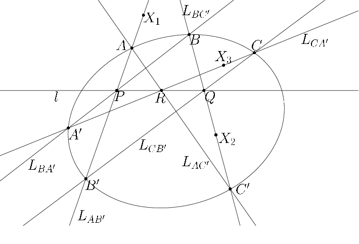
Construction of the hypothesis $H$ :
Input: points $A,B,C,X_{1},X_{2},X_{3}$ , line $l$ . Depth 1: lines $L_{AB^{\prime}}=\overline{AX_{1}}$ , $L_{BC^{\prime}}=\overline{BX_{2}}$ , $L_{CA^{\prime}}=\overline{CX_{3}}$ . Depth 2: points $P=L_{AB^{\prime}}\cap l$ , $Q=L_{BC^{\prime}}\cap l$ , $R=L_{CA^{\prime}}\cap l$ . Depth 3: lines $L_{AC^{\prime}}=\overline{AR}$ , $L_{BA^{\prime}}=\overline{BP}$ , $L_{CB^{\prime}}=\overline{CQ}$ . Depth 4: points $A^{\prime}=L_{CA^{\prime}}\cap L_{BA^{\prime}},B^{\prime}=L_{AB^{\prime}}\cap L_{CB^{\prime}},$ $C^{\prime}=L_{AC^{\prime}}\cap L_{BC^{\prime}}$ . Thesis node: conic $R$ .
Thesis: points $A,B,C,A^{\prime},B^{\prime},C^{\prime}$ belong to conic $R$ .

4.1.4 Chasles Theorem

Chasles Theorem [7] states that if $\{q_{1},\ldots,q_{9}\}$ are the intersection points of two cubics, then any cubic passing through $\{q_{1},\ldots,q_{8}\}$ also passes through $q_{9}$ . This implies that given another free point $q_{0}$ , there is always a cubic through $\{q_{0},q_{1},\ldots,q_{9}\}$ . This version can be easily translated to the tropical context.

Theorem 48 (Chasles Theorem).

Construction of the hypothesis $H$ :
Input: cubics $C_{1}$ , $C_{2}$ , point $q_{0}$ . Depth 1: points $\{q_{1},\ldots,q_{9}\}=C_{1}\cap C_{2}$ . Thesis node: cubic $R$ .
Thesis: points $\{q_{0},q_{1},\ldots,q_{9}\}$ belong to cubic $R$ .

It is not true that every cubic passing through eight of the intersection points passes through the ninth. See Figure 5. Let $f=``0+1x+1y+1x^{2}+3xy+1y^{2}+0x^{3}+1x^{2}y+1xy^{2}+0y^{3}$ , $g=19+14x+20xy+24y+7x^{2}+12x^{2}y+23xy^{2}+28y^{2}+0x^{3}+31y^{3}"$ ,

\begin{matrix}f\cap_{st}g=&\{(-1,-3),&(0,-3),&(1,-3),\phantom{\}}\\ &\phantom{\{}(-1,-4),&(0,-4),&(1,-4),\phantom{\}}\\ &\phantom{\{}(-1,-5),&(0,-5),&(1,-5)\phantom{,}\}\end{matrix}

Take $h=``0+1x+5y+\frac{11}{2}xy+1x^{2}+9y^{2}+5x^{2}y+9xy^{2}+0x^{3}+12y^{3}"$ . This is a cubic passing through $8$ of the stable intersection points of $f$ and $g$ but not through the ninth.

An alternative to the Chasles Theorem that also holds in the tropical plane is the following. Take as $8+n$ points $\{q_{1},\ldots,q_{8}\}$ , $\{x_{1},\ldots,x_{n}\}$ , $n\geq 3$ . All the steps are computing the cubic $C_{i}$ passing through $\{q_{1},\ldots,q_{8},x_{i}\}$ , $1\leq i\leq n$ . The thesis node is a point $x$ and the thesis is that $x$ belongs to $C_{i}$ , $1\leq i\leq n$ . The difference with the previous version of Chasles theorem is that, by construction, the eight points $\{q_{1},\ldots,q_{8}\}$ are always in general position in every cubic $C_{i}$ . In our example, the points are not in general position neither in $\mathcal{T}(f)$ nor $\mathcal{T}(g)$ .

An immediate generalization of Chasles Theorem is the following.

4.1.5 Cayley-Bacharach Theorem

The generalization of Chasles Theorem (cf [7]) we discuss here is the following: let $C_{1}$ , $C_{2}$ be plane curves of degrees d and e respectively, intersecting in $de$ distinct points $Q=\{p_{1},\ldots,p_{de}\}$ . If $C$ is any plane curve of degree $d+e-3$ containing all but one point of $Q$ , then $C$ contains every point of $Q$ . The second version of Chasles Theorem given does not fit well to this theorem, but the generalization of the first version of Chasles Theorem is immediate, note that a curve of $d+e-3$ is determined by $\frac{d^{2}+e^{2}-3e-3d}{2}$ points:

Let $d,e\geq 3$ natural numbers, $l=1+\frac{d^{2}+e^{2}-3e-3d}{2}$

Theorem 49 (Cayley-Bacharach Theorem).

Construction of the hypothesis $H$ :
Input: degree $d$ curve $C_{1}$ , degree $e$ curve $C_{2}$ , points $p_{1},\ldots,p_{l}$ . Depth 1: points $\{q_{1},\ldots,q_{de}\}=C_{1}\cap C_{2}$ . Thesis node: curve $R$ of degree $d+e-3$ .
Thesis: points $\{q_{1},\ldots,q_{de}\}\cup\{p_{1},\ldots,p_{l}\}$ belong to curve $R$ .

4.1.6 Weak Pascal Theorem

This Theorem is not in the context of Theorem 44 because the construction involved is not admissible. Nevertheless, for some tropical realization of the hypothesis, we will be in the context of Theorem 38. So this Theorem does not hold for every tropical input, we have to add conditions in the tropical realization.

Theorem 50 (Weak Pascal Theorem).

Consider the following construction:
Input: conic $Z$ , lines $L_{1}$ , $L_{2}$ , $L_{3}$ . Depth 1: points $\{A,B^{\prime}\}=R\cap L_{1}$ , $\{B,C^{\prime}\}=R\cap L_{2}$ , $\{C,A^{\prime}\}=R\cap L_{3}$ . Depth 2: lines $L_{4}=\overline{AC^{\prime}}$ , $L_{5}=\overline{BA^{\prime}}$ , $L_{6}=\overline{CB^{\prime}}$ . Depth 3: points $P=L_{1}\cap L_{5}$ , $Q=L_{2}\cap L_{6}$ , $R=L_{3}\cap L_{4}$ .
If a tropical instance of this construction is such that each set of points $\{A,C^{\prime}\}$ , $\{B,A^{\prime}\}$ and $\{C,B^{\prime}\}$ is in generic position with respect to $Z$ , then there is a line $L$ (thesis node) that contains the points $P$ , $Q$ and $R$ .

Proof.

This construction, in the algebraic context, provides instances of Pascal theorem. Hence, if the input is generic, then points $\widetilde{P}$ , $\widetilde{Q}$ , $\widetilde{R}$ are collinear. But this construction is not admissible, so Theorem 44 does not apply. Nevertheless, this construction is in the context of Theorem 38. The minimal multiples paths are $Z\rightrightarrows L_{4}$ , $Z\rightrightarrows L_{5}$ and $Z\rightrightarrows L_{6}$ . By Theorem 38, if each one of these three sets is in general position with respect to $R$ , then this tropical instance can be lifted to the a generic instance in the algebraic framework. As Pascal Theorem holds in $\mathbb{K}$ . $\widetilde{P}$ , $\widetilde{Q}$ and $\widetilde{R}$ are collinear. So $P$ , $Q$ and $R$ will be collinear. ∎

Example 51.

Let $Z=``3y+5+3y^{2}+0x^{2}+4x+0xy"$ $L_{1}=``1y+0x+0"$ $L_{2}=``0y+0x+2"$ $L_{3}=``(9/2)y+0x+3"$ , then $A=(3,2)$ , $B^{\prime}=(1,0)$ , $B=C^{\prime}=(2,3/2)$ , $C=(1,-3/2)$ , $A^{\prime}=(4,-1/2)$ , $L_{4}=``3y+2x+(9/2)"$ , $L_{5}=(3/2)x+4y+(11/2)$ , $L_{6}=0x+1y+1$ , $P=(5/2,3/2)$ , $Q=(2,1)$ , $R=(5/2,-3/2)$ . The points $P$ , $Q$ and $R$ are not collinear, in this example, the set $\{C,B^{\prime}\}$ is not in generic position in $Z$ .

However, for these input elements, the election of the points in the depth 1 steps is arbitrary. If we now take $A=(1,0)$ , $B^{\prime}=(3,2)$ , $B=C^{\prime}=(2,3/2)$ , $C=(4,-1/2)$ and $A^{\prime}=(1,-3/2)$ , now $L_{4}=``2y+(3/2)x+(5/2)"$ , $L_{5}=``2y+(3/2)x+(5/2)"$ , $L_{6}=``4y+2x+6"$ , $P=(1,0)$ , $Q=(2,2)$ , $R=(1,-3/2)$ . In this case, the three sets of points are in generic position in $Z$ , it can be checked that the three points belong to the tropical line of equation $L=``2x+2y+3"$ .

References

[1] Bernstein, D. N., 1975. The number of roots of a system of equations. Akademija Nauk SSSR. Funkcional^′ nyi Analiz i ego Priloženija 9 (3), 1–4.
[2] Bogart, T., Jensen, A. N., Speyer, D., Sturmfels, B., Thomas, R. R., 2007. Computing tropical varieties. J. Symbolic Comput. 42 (1-2), 54–73.
[3] Chou, S.-C., 1988. Mechanical geometry theorem proving. Vol. 41 of Mathematics and its Applications. D. Reidel Publishing Co., Dordrecht, with a foreword by Larry Wos.
[4] Dembowski, P., 1968. Finite geometries. Ergebnisse der Mathematik und ihrer Grenzgebiete, Band 44. Springer-Verlag, Berlin.
[5] Develin, M., Santos, F., Sturmfels, B., 2005. On the rank of a tropical matrix. In: Combinatorial and computational geometry. Vol. 52 of Math. Sci. Res. Inst. Publ. Cambridge Univ. Press, Cambridge, pp. 213–242.
[6] Einsiedler, M., Kapranov, M., Lind, D., 2006. Non-Archimedean amoebas and tropical varieties. J. Reine Angew. Math. 601, 139–157.
[7] Eisenbud, D., Green, M., Harris, J., 1996. Cayley-Bacharach theorems and conjectures. American Mathematical Society. Bulletin. New Series 33 (3), 295–324.
[8] Gathmann, A., Markwig, H., 2007. The numbers of tropical plane curves through points in general position. J. Reine Angew. Math. 602, 155–177.
[9] Gel^′fand, I. M., Kapranov, M. M., Zelevinsky, A. V., 1990. Newton polytopes of the classical resultant and discriminant. Advances in Mathematics 84 (2), 237–254.
[10] Jensen, A. N., Markwig, H., Markwig, T., 2007. An algorithm for lifting points in a tropical variety. Preprint.
[11] Kuhlmann, F.-V., Lombardi, H., Perdry, H., 2003. Dynamic computations inside the algebraic closure of a valued field. In: Valuation theory and its applications, Vol. II (Saskatoon, SK, 1999). Vol. 33 of Fields Inst. Commun. Amer. Math. Soc., Providence, RI, pp. 133–156.
[12] Kushnirenko, A., 1976. Newton polytopes and the bezout theorem. Functional Analysis and Its Applications 10 (3), 233–235.
[13] Markwig, H., July 2006. The enumeration of plane tropical curves. Ph.D. thesis, Technische Universität Kaiserslautern.
[14] Mikhalkin, G., 2005. Enumerative tropical algebraic geometry in $\mathbb{R}^{2}$ . Journal of the American Mathematical Society 18 (2), 313–377 (electronic).
[15] Richter-Gebert, J., Sturmfels, B., Theobald, T., 2005. First steps in tropical geometry. In: Idempotent mathematics and mathematical physics. Vol. 377 of Contemp. Math. Amer. Math. Soc., Providence, RI, pp. 289–317.
[16] Robinson, A., 1956. Complete theories. North-Holland Publishing Co., Amsterdam.
[17] Rojas, J. M., 1999. Toric intersection theory for affine root counting. Journal of Pure and Applied Algebra 136 (1), 67–100.
[18] Sturmfels, B., 1994. On the Newton polytope of the resultant. Journal of Algebraic Combinatorics. An International Journal 3 (2), 207–236.
[19] Tabera, L. F., 2005. Tropical constructive Pappus’ theorem. International Mathematics Research Notices 2005 (39), 2373–2389.
[20] Tabera, L. F., 2006. Constructive proof of extended kapranov theorem. In: Actas del X Encuentro de Álgebra Computacional y Aplicaciones, EACA 2006. pp. 178–181.
[21] Tabera, L. F., 2007. Tropical resultants for curves and stable intersection. Manuscript.
[22] Thaler, A. I., 1964. On the Newton polytope. Proceedings of the American Mathematical Society 15, 944–950.
[23] Vigeland, M. D., 2006. Tropical fano theorem. Personal communication.

Luis Felipe Tabera Alonso
Dept. Àlgebra i Geometria, Facultat de Matemàtiques, Universitat de Barcelona
Barcelona, Spain
e-mail: tabera@ub.edu