Quasi-isometries and rigidity of solvable groupsThanks: First author partially supported by NSF grant DMS-0244542. Second author partially supported by NSF grants DMS-0226121 and DMS-0541917. Third author partially supported by NSF grant DMS-0349290 and a Sloan Foundation Fellowship.
Abstract.
In this note, we announce the first results on quasi-isometric rigidity of non-nilpotent polycyclic groups. In particular, we prove that any group quasi-isometric to the three dimenionsional solvable Lie group is virtually a lattice in . We prove analogous results for groups quasi-isometric to where the semidirect product is defined by a diagonalizable matrix of determinant one with no eigenvalues on the unit circle. Our approach to these problems is to first classify all self quasi-isometries of the solvable Lie group. Our classification of self quasi-isometries for proves a conjecture made by Farb and Mosher in [FM3].
Our techniques for studying quasi-isometries extend to some other classes of groups and spaces. In particular, we characterize groups quasi-isometric to any lamplighter group, answering a question of de la Harpe [dlH]. Also, we prove that certain Diestel-Leader graphs are not quasi-isometric to any finitely generated group, verifying a conjecture of Diestel and Leader from [DL] and answering a question of Woess from [SW, Wo1]. We also prove that certain non-unimodular, non-hyperbolic solvable Lie groups are not quasi-isometric to finitely generated groups.
The results in this paper are contributions to Gromov’s program
for classifying finitely generated groups up to quasi-isometry
[Gr2]. We introduce a new technique for studying
quasi-isometries, which we refer to as coarse
differentiation.
Dedicated to Gregory Margulis on the occasion of his th birthday.
1. Introduction and statements of rigidity results
For any group generated by a subset one has the associated Cayley graph, . This is the graph with vertex set and edges connecting any pair of elements which differ by right multiplication by a generator. There is a natural action on by left translation. By giving every edge length one, the Cayley graph can be made into a (geodesic) metric space. The distance on viewed as the vertices of the Cayley graph is the word metric, defined via the norm:
Different sets of generators give rise to different metrics and Cayley graphs for a group but one wants these to be equivalent. The natural notion of equivalence in this category is quasi-isometry:
Definition 1.1.
Let and be metric spaces. Given real numbers and ,a map is called a -quasi-isometry if
- (1)
for all and in , and,
- (2)
the neighborhood of is all of .
If is a finitely generated group, is canonically quasi-isometric to any finite index subgroup in and to any quotient for any finite normal subgroup . The equivalence relation generated by these (trivial) quasi-isometries is called weak commensurability. A group is said to virtually have a property if some weakly commensurable group does.
In his ICM address in 1983, Gromov proposed a broad program for studying finitely generated groups as geometric objects, [Gr2]. Though there are many aspects to this program (see [Gr3] for a discussion), the principal question is the classification of finitely generated groups up to quasi-isometry. By construction, any finitely generated group is quasi-isometric to any space on which acts properly discontinuously and cocompactly by isometries. For example, the fundamental group of a compact manifold is quasi-isometric to the universal cover of the manifold (this is called the Milnor-Svarc lemma). In particular, any two cocompact lattices in the same Lie group are quasi-isometric. One important aspect of Gromov’s program is that it allows one to generalize many invariants, techniques, and questions from the study of lattices to all finitely generated groups.
Given the motivations coming from the study of lattices, one of the first questions in the field is whether a group quasi-isometric to a lattice is itself a lattice, at least virtually. This question has been studied extensively. For lattices in semisimple groups this has been proven, see particularly [P1, S1, FS, S2, KL, EF, E] and also the survey [F] for further references. For lattices in other Lie groups the situation is less clear. It follows from Gromov’s polynomial growth theorem [Gr1] that any group quasi-isometric to a nilpotent group is virtually nilpotent, and hence essentially a lattice in some nilpotent Lie group. However, the quasi-isometry classification of lattices in nilpotent Lie groups remains an open problem.
In the case of solvable groups, even less is known. The main motivating question is the following:
Conjecture 1.2.
Let be a solvable Lie group, and let be a lattice in . Any finitely generated group quasi-isometric to is virtually a lattice in a (possibly different) solvable Lie group .
Remarks:
- (1)
As solvable Lie groups have only cocompact lattices, studying groups quasi-isometric to lattices in is equivalent to studying groups quasi-isometric to .
- (2)
- (3)
Conjecture 1.2 can be rephrased to make no reference to connected Lie groups. In particular, by a theorem of Mostow, any polycyclic group is virtually a lattice in a solvable Lie group, and conversely any lattice in a solvable Lie group is virtually polycyclic [Mo2]. The conjecture is equivalent to saying that any finitely generated group quasi-isometric to a polycyclic group is virtually polycyclic. This means that being polycyclic is a geometric property.
- (4)
Erschler has shown that a group quasi-isometric to a solvable group is not necessarily virtually solvable [D]. Thus, the class of virtually solvable groups is not closed under the equivalence relation of quasi-isometry. In other words, solvability is not a geometric property.
- (5)
Some classes of solvable groups which are not polycyclic are known to be quasi-isometrically rigid. See particularly the work of Farb and Mosher on the solvable Baumslag-Solitar groups [FM1, FM2] as well as later work of Farb-Mosher, Mosher-Sageev-Whyte and Wortman [FM3, MSW, W]. The methods used in all of these works depend essentially on topological arguments based on the explicit structure of singularities of the spaces studied and cannot apply to polycyclic groups.
- (6)
Our main results establish Conjecture 1.2 in many cases. We believe our techniques provide a method to attack the conjecture. This is work in progress, some of it joint with Irine Peng.
From an algebraic point of view, solvable groups are generally easier to study than semisimple ones, as the algebraic structure is more easily manipulated. In the present context it is extremely difficult to see that any algebraic structure is preserved and so we are forced to work geometrically. For nilpotent groups the only geometric fact needed is polynomial volume growth. For semisimple groups, the key fact for all approaches is nonpositive curvature. The geometry of solvable groups is quite difficult to manage, since it involves a mixture of positive and negative curvature as well as exponential volume growth.
The simplest non-trivial example for Conjecture 1.2 is the -dimensional solvable Lie group . This example has received a great deal of attention. The group with acting on via the diagonal matrix with entries and . As matrices, can be written as :
The metric is a left invariant metric on . Any group of the form for with is a cocompact lattice in .
The following theorem proves a conjecture of Farb and Mosher and is one of our main results:
Theorem 1.3.
Let be a finitely generated group quasi-isometric to . Then is virtually a lattice in .
More generally, we can describe the quasi-isometry types of lattices in many solvable groups. Here we restrict our attention to groups of the form where the action of on is given by powers of an by matrix . The following theorem proves another conjecture of Farb and Mosher.
Theorem 1.4.
Suppose is a positive definite symmetric matrix with no eigenvalues equal to one, and . If is a finitely generated group quasi-isometric to , then is virtually a lattice in for some .
Remarks:
- (1)
This theorem is deduced from Theorem 2.2 below and a theorem from the Ph.d. thesis of T. Dymarz.
- (2)
This result is best possible. All the Lie groups for in are quasi-isometric.
The following is a basic question:
Question 1.5.
Given a Lie group , is there a finitely generated group quasi-isometric to ?
It is clear that the answer is yes whenever has a cocompact lattice. However, many solvable locally compact groups, and in particular, many solvable Lie groups do not have any lattices. The simplest examples are groups which are not unimodular. However, it is possible for Question 1.5 to have an affirmative answer even if is not unimodular. For instance, the non-unimodular group solvable group acts simply transitively by isometries on the hyperbolic plane, and thus is quasi-isometric to the fundamental group of any closed surface of genus at least . Thus the answer to Question 1.5 can be subtle. Our methods give:
Theorem 1.6.
Let be a solvable Lie group where the action on is defined by for , . Then there is no finitely generated group quasi-isometric to .
If and , then admits a left invariant metric of negative curvature. The fact that there is no finitely generated group quasi-isometric to in this case is a result of Kleiner [K], see also [P2]. Both our methods and Kleiner’s prove similar results for groups of the form . Nilpotent Lie groups not quasi-isometric to any finitely generated group where constructed in [ET].
In addition our methods yield quasi-isometric rigidity results for a variety of solvable groups which are not polycyclic, in particular the so-called lamplighter groups. These are the wreath products where is a finite group. The name lamplighter comes from the description where the action is by a shift. The subgroup is thought of as the states of a line of lamps, each of which has states. The ”lamplighter” moves along this line of lamps (the action) and can change the state of the lamp at her current position. The Cayley graphs for the generating sets depend only on , not the structure of . Furthermore, and are quasi-isometric whenever there is a so that and for some in . The problem of classifying these groups up to quasi-isometry, and in particular, the question of whether the and state lamplighter groups are quasi-isometric, were well known open problems in the field, see [dlH].
Theorem 1.7.
The lamplighter groups and are quasi-isometric if and only if there exist positive integers such that and .
For a rigidity theorem for lamplighter groups, see Theorem 1.8 below.
To state Theorem 1.8 as well as an analogue of Theorem 1.6 for groups which are not Lie groups, we need to describe a class of graphs. These are the Diestel-Leader graphs, , which can be defined as follows: let and be regular trees of valence and . Choose orientations on the edges of and so each vertex has (resp. ) edges pointing away from it. This is equivalent to choosing ends on these trees. We can view these orientations at defining height functions and on the trees (the Busemann functions for the chosen ends). If one places the point at infinity determining at the top of the page and the point at infinity determining at the bottom of the page, then the trees can be drawn as:

The graph is the subset of the product defined by . The analogy with the geometry of is made clear in section 3. For the Diestel-Leader graphs arise as Cayley graphs of lamplighter groups for . This observation was apparently first made by R.Moeller and P.Neumann [MN] and is described explicitly, from two slightly different points of view, in [Wo2] and [W]. We prove the following:
Theorem 1.8.
Let be a finitely generated group quasi-isometric to the lamplighter group . Then there exists positive integers such that and an isometric, proper, cocompact action of a finite index subgroup of on the Diestel-Leader graph .
Remark: The theorem can be reinterpreted as saying that any group quasi-isometric to is virtually a cocompact lattice in the isometry group of where is as above.
In [SW, Wo1], Soardi and Woess ask whether every homogeneous graph is quasi-isometric to a finitely generated group. The graph is easily seen to be homogeneous (i.e. it has a transitive isometry group). For its isometry group is not unimodular, and hence has no lattices. Thus there are no obvious groups quasi-isometric to in this case. In fact, we have:
Theorem 1.9.
There is no finitely generated group quasi-isometric to the graph for .
This theorem was conjectured by Diestel and Leader in [DL], where the Diestel-Leader graphs were introduced for this purpose. Note that Theorem 1.9 can be reinterpreted as the statement that for , there is no finitely generated group quasi-isometric to the isometry group of .
All our theorems stated above are proved using a new technique, which we call coarse differentiation. Even though quasi-isometries have no local structure and conventional derivatives do not make sense, we essentially construct a “coarse derivative” that models the large scale behavior of the quasi-isometry. This construction is quite different from the conventional method of passing to the asymptotic cone, see §4.4 for more discussion.
We now state a theorem that is a well-known consequence of Theorem 1.3, Thurston’s Geometrization Conjecture and results in [CC, Gr1, KaL1, KaL2, PW, S1, Ri]. We state it assuming that the Geometrization Conjecture is known.
Theorem 1.10.
Let be a compact three manifold without boundary and a finitely generated group. If is quasi-isometric to the universal cover of , then is virtually the fundamental group of , also a compact three manifold without boundary.
2. Quasi-isometries are height respecting
A typical step in the study of quasi-isometric rigidity of groups is the identification of all quasi-isometries of some space quasi-isometric to the group, see §4.6 for a brief explanation. For us, the space is either a solvable Lie group or . In all of these examples there is a special function which we call the height function and a foliation of by level sets of the height function. We will call a quasi-isometry of any of these spaces height respecting if it permutes the height level sets to within bounded distance (In [FM4], the term used is horizontal respecting).
For , the height function is .
Theorem 2.1.
Any -quasi-isometry of is within bounded distance of a height respecting quasi-isometry . Furthermore, this distance can be taken uniform in and therefore, in particular, is a -quasi-isometry where depend only on and .
Remark: In fact, Theorem 2.1 can be used to identify the quasi-isometries of completely. Possibly after composing with the map , any height respecting quasi-isometry (and in particular, any isometry) is at bounded distance from a quasi-isometry of the form where and are bilipschitz functions. Given a metric space , one defines to be the group of quasi-isometries of modulo the subgroup of those at finite distance from the identity. The previous statement can then be taken to mean that . This explicit description was conjectured by Farb and Mosher.
If we take a group of the form as in Theorem 1.4, we can write coordinates where is the coordinate in and is the coordinate in . Here and level sets of are cosets.
Theorem 2.2.
Let be as in Theorem 1.4. Then any -quasi-isometry of is within a bounded distance of a height respecting quasi-isometry . Furthermore, the bound is uniform in and .
Remark: There is an explicit description of in this context as well, but it is somewhat involved so we omit it.
Recall that is defined as the subset of where where and are Busemann functions on and respectively. Here we simply set which makes sense exactly on . The reader can verify that the level sets of the height function are orbits for a subgroup of .
Theorem 2.3.
Any -quasi-isometry of is within bounded distance from a height respecting quasi-isometry . Furthermore, the bound is uniform in and .
Remark: We can reformulate Theorem 2.3 in terms similar to those of Theorem 2.1. Here the group will be replaced by for (resp. ) the complement of a point in the (visual) boundary of (resp. ). These can easily be seen to be the -adic and -adic rationals, respectively.
Note that when , this theorem is used to prove Theorem 1.8 and when it is used to prove Theorem 1.9. The proofs in these two cases are somewhat different, the proof in the case being almost identical to the proof of Theorem 2.1. In the other case, the argument is complicated by the absence of metric Fölner sets, but simplifications also occur since there is no element in the isometry group that “flips” height, see the remarks in §4.5.
There is an analogue of the above results for the case of the solvable groups which appear in Theorem 1.6.
3. Geometry of
In this subsection we describe the geometry of and related spaces in more detail, with emphasis on the geometric facts used in our proofs.
The upper half plane model of the hyperbolic plane is the set with the length element . If we make the change of variable , we get with the length element . This is the log model of the hyperbolic plane .
The length element of is:
Thus planes parallel to the plane are hyperbolic planes in the log model. Planes parallel to the plane are upside-down hyperbolic planes in the log model. All of these copies of are isometrically embedded and totally geodesic .
We will refer to lines parallel to the -axis as -horocycles, and to lines parallel to the -axis as -horocycles. This terminology is justified by the fact that each ( or )-horocycle is indeed a horocycle in the hyperbolic plane which contains it.
We now turn to a discussion of geodesics and quasi-geodesics in . Any geodesic in an leaf in is a geodesic. There is a special class of geodesics, which we call vertical geodesics. These are the geodesics which are of the form or . We call the vertical geodesic upward oriented in the first case, and downward oriented in the second case. In both cases, this is a unit speed parametrization. Each vertical geodesic is a geodesic in two hyperbolic planes, the plane and the plane .
Certain quasi-geodesics in are easy to describe. Given two points and , there is a geodesic in the hyperbolic plane that joins to and a geodesic in the plane that joins to a . It is easy to check that the concatenation of and is a quasi-geodesic. In first matching the coordinates and then matching the coordinates, we made a choice. It is possible to construct a quasi-geodesic by first matching the coordinates and then the coordinates. This immediately shows that any pair of points not contained in a hyperbolic plane in can be joined by two distinct quasi-geodesics which are not close together. This is an aspect of positive curvature. One way to prove that the objects just constructed are quasi-geodesics is to note the following: The pair of projections onto the and coordinate planes can be combined into a quasi-isometric embedding .
We state here the simplest version of a key geometric fact used at various steps in the proof.
Lemma 3.1 (Quadrilaterals).
Suppose and are vertical geodesic segments parametrized by arclength. Suppose . Assume that for , ,
so that connects the -neighborhood of to the -neighborhood of . Further assume that for and all , (so that for each , the two segments leaving the neighborhood of diverge right away). Then there exists depending only on such that exactly one of the following holds:
- (a)
All four are upward oriented, is within of the -horocycle passing through and is within of the -horocycle passing through .
- (b)
All four are downward oriented, is within of the -horocycle passing through and is within of the -horocycle passing through .
We think of and as defining a quadrilateral. The content of the lemma is that any quadrilateral has its four ”corners” in pairs that lie essentially along horocycles. In particular, if we take a quadrilateral with geodesic segments and with and and map it forward under a -quasi-isometry , and if we would somehow know that sends each of the four close to a vertical geodesic, then Lemma 3.1 would imply that sends the (resp. ) to a pair of points at roughly the same height.
We now define certain useful subsets of . Let . Then and , so is a Fölner set. We call a box of size centered at the identity. We define the box of size centered at a point by where is left translation by . Since left translation is an isometry, is also a Fölner set. We frequently omit the center of a box in our notation and write .
Notice that the top of , meaning the set , is not at all square - the sides of this rectangle are horocyclic segments of lengths and - in other words it is just a small metric neighborhood of a horocycle. Similarly, the bottom is also essentially a horocycle but in the transverse direction. Further, we can connect the -neighborhood of any point of the top horocycle to the -neighborhood of any point of the bottom horocycle by a vertical geodesic segment, and these segments essentially sweep out the box . Thus a box contains an extremely large number of quadrilaterals. This picture is even easier to understand in the Diestel-Leader graphs , where the boundary of the box is simply the union of the top and bottom ”horocycles”, and the vertical geodesics in the box form a complete bipartite graph between the two.
We remark that for the group in Theorem 1.6, and for the graphs for , one has boxes with essentially the same definition, but these will not be a (metric) Fölner set. A solvable Lie group admits metric Fölner sets if and only if it is unimodular. The same is true of graphs. While the isometry group of a graph is always amenable, the graph only has metric Fölner sets if the isometry group is unimodular.
4. On proofs
In this section, we give some of the key ideas in the proofs. In the first two subsections we indicate the key new ideas behind our proof of Theorem 2.1. The first contains quantative estimates on the behavior of quasi-geodesics. The second subsection averages this behavior over families of quasi-geodesics. In §4.3 we sketch the proof of Theorem 2.1. Before continuing with discussion of proofs, we include a discussion of how to axiomatize the methods of §4.1 and §4.2 into a general method of coarse differentiation in §4.4. Subsection 4.5 briefly discusses the ideas needed to adapt the proof of Theorem 2.1 to prove the other results in Section 2. In subsection §4.6, we discuss deducing results in §1 from results in §2.
4.1. Behavior of quasi-geodesics
We begin by discussing some quantative estimates on the behavior of quasi-geodesic segments in . Throughout the discussion we assume is a -quasi-geodesic segment for a fixed choice of , i.e. is a quasi-isometric embedding of into . A quasi-isometric embedding is a map that satisfies point in Definition 1.1 but not point .
Definition 4.1 (-monotone).
A quasigeodesic segment is -monotone if for all with we have .

The following fact about -monotone geodesics is an easy exercise in hyperbolic geometry:
Lemma 4.2 (-monotone is close to vertical).
If is -monotone, then there exists a vertical geodesic segment such that .
Remark: The distance is the Hausdorff distance between the sets and does not depend on parametrizations.
Lemma 4.3 (Subdivision).
Suppose is a quasi-geodesic segment which is not -monotone. Suppose (depending on , , ). Then
Outline of Proof. If is sufficiently large, the total variation of the height increases after the subdivision by a term proportional to . See Figure 3. ∎

Choosing Scales: Choose . In particular, and .
Lemma 4.4.
Suppose , and suppose is a quasi-geodesic segment. For each , subdivide into segments of length . Let denote the fraction of these segments whose images are not -monotone. Then,
Proof. By applying Lemma 4.3 to each non--monotone segment on the scale , we get
Doing this again, we get after iterations,
But the left-hand-side is bounded from above by the length and so bounded above by . ∎
4.2. Averaging
In this subsection we apply the estimates from above to images of geodesics under a quasi-isometry of . The idea is to average the previous estimates over families of quasi-geodesics. This results in a coarse analogue of Rademacher’s theorem, which says that a bilipschitz map of is differentiable almost everywhere, see below for discussion.
Setup and Notation.
- •
Suppose is a quasi-isometry. Without loss of generality, we may assume that is continuous.
- •
Let be a vertical geodesic segment parametrized by arclength where .
- •
Let . Then is a quasi-geodesic segment.
It follows from Lemma 4.4, that for every and every geodesic segment , assuming that is sufficiently large, there exists such that . The difficulty is that may depend on . For , this is overcome as follows:
Recall that . Then and , so is a Fölner set. Average the result of Lemma 4.4 over , the set of vertical geodesics in and let denote the measure/cardinality of . Changing order, we get:

Thus, given any , (by choosing sufficiently large) we can make sure that there exists such that
| (1) |
Conclusion. On the scale , at least fraction of all vertical geodesic segments in have nearly vertical images under . See Figure 4.
The difficulty is that, at this point, it may be possible that some of the (upward oriented) vertical segments in may have images which are going up, and some may have images which are going down.
We think of the process we have just described as a form of “coarse differentiation”. For further discussion of this process and a more general variant on the discussion in the last two subsections, see subsection 4.4.
4.3. The scheme of the proof of Theorem 2.1.
Roughly speaking, the proof proceeds in the following steps:
Step 1.
For all there exists such that for any box where , there exists such that for the tiling:
there exists with and for each there exists a height-respecting map and a subset with such that
Roughly, Step 1 asserts that every sufficiently large box can be tiled into small boxes, in such a way that for most of the small boxes , the restriction of to agrees, on most of the measure of , with a height-respecting map . There is no assertion in Step 1 that the height-respecting maps on different small boxes match up to define a height-respecting map on most of the measure on ; the main difficulty is that some of the may send the “up” direction to the “down” direction, while other may preserve the up direction.
Step 1 follows from a version of (1) and some geometric arguments using Lemma 3.1. The point is that any -monotone quasi-geodesic is close to a vertical geodesic by Lemma 4.2. By the averaging argument in subsection 4.2, we find a scale at which most segments have -monotone image under . More averaging implies that on most boxes most geodesic segments joining the top of the box to the bottom of the box have -monotone images. We then apply Lemma 3.1 to the images of these geodesics and use this to show that the map is roughly height preserving on each . This step also uses the geometric description of given in the next to last paragraph of §3, i.e. the fact that a box is coarsely a complete bipartite graphs on nets in the “top” and “bottom” of the box.
Step 2.
For all there exists such that for any box where , subset with and a height-respecting map such that
where .
This is the essentially the assertion that the different maps from Step 1 are all oriented in the same way, and can thus be replaced by one standard map .
Step 2 is the most technical part of the proof. The problem here derives from exponential volume growth. In Euclidean space, given a set of almost full measure in a box, every point in the box is close to a point in . This is not true in because of exponential volume growth. Another manifestation of this difficulty is that does not have a Besicovitch covering lemma. The proof involves using refinements of Lemma 3.1 and further averaging on the image of .
Step 3.
The map is from a standard map .
4.4. Remarks on coarse differentiation:
If a map is differentiable, then it is locally at sub-linear error from a map which takes lines to lines. This is roughly the conclusion of the argument above for the vertical geodesics in , at least on an appropriately chosen large scale and off of a set of small measure. The ideas employed here can be extended to general metric spaces, by replacing the notion of -monotone with a more general notion of -efficient which we will describe below. The ideas in our proof are not so different from the proof(s) of Rademacher’s theorem that a bilipschitz map of is differentiable almost everywhere. In fact, our method applied to quasi-isometries of gives roughly the same information as the application of Rademacher’s theorem to the induced bilipschitz map on the asymptotic cone of (which is again ). In this context the presence of sets of small measure can be eliminated by a covering lemma argument. In the context of solvable groups, passage to the asymptotic cone is complicated by the exponential volume growth. The asymptotic cone for these groups is not locally compact, which makes it difficult to find useful notions of sets of zero or small measure there.
We now formulate somewhat loosely a more general form of the “differentiation theorem” given in subsections 4.1 and 4.2. Throughout this subsection will be a general metric space, though it may be most useful to think of as a complete, geodesic metric space. First we generalize the notion of -monotone.
Definition 4.5.
A quasigeodesic segment is -efficient on the scale if
The fact is that a quasi-geodesic, unless it is a quasi-geodesic, fails to be -efficient at some scale some fraction of the time. The observation embedded in subsection 4.1 is that this cannot happen everywhere on all scales and in fact cannot happen too often on too many scales.
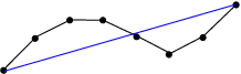
With this definition, the following variant on Lemma 4.3 becomes a tautology.
Lemma 4.6 (Subdivision II).
Given , there exist and (depending on and ) such that any -quasi-geodesic segment which is not -efficient on scale we have:
We now state a variant of Lemma 4.4 whose proof is verbatim the proof of that lemma.
Choosing Scales: Choose . In particular, and .
Lemma 4.7.
Suppose , and suppose is a quasi-geodesic segment. For each , subdivide into segments of length . Let denote the fraction of these segments whose images are not -efficient on scale . Then,
Let be a geodesic metric space. Coarse differentiation amounts to the following easy lemma.
Lemma 4.8 (Coarse Differentiation).
Let be a -quasi-isometry. For all there exists such that for any and any family of geodesics of length in , there exist scales with such that if we divide each geodesic in into subsegments of length , then at least fraction of these subsegments have images which are -efficient at scale .
This lemma and its variants seem likely to be useful in other settings. In fact, the lemma holds only assuming that is coarsely lipschitz. A map is a coarsely lipschitz if . We now describe the relation to taking derivatives and also to the process of taking a “derivative at infinity” of a quasi-isometry by passing to asymptotic cones.
We first discuss the case of maps . Suppose is a quasi-isometry. Suppose one chooses a net on the unit circle and takes to be the set of all lines of length in a large box, whose direction vector is in . Lemma 4.8 applied to then states that most of these lines, on the appropriate scale, map under close to straight lines, which implies that the map (in a suitable box) can be approximated by an affine map. Thus, in this context, Lemma 4.8 is indeed analogous to differentiation (or producing points of differentiability).
An alternative approach for analyzing quasi-isometries is to pass to the asymptotic cone to obtain a bilipschitz map and then apply Rademacher’s theorem to . If one attempts to pull the information this yields back to one gets statements that are similar to those one would obtain directly using Lemma 4.8. This is not surprising, since averaging arguments like those used in the proof of Lemma 4.8 are implicit in the proofs of Rademacher’s theorem.
Passing to the asymptotic cone has obvious advantages because it allows one to replace a quasi-isometry from to with a -quasi-isometry (i.e. a bilipschitz map) from the asymptotic cone of to the asymptotic cone of . One can then try to use analytic techniques to study the bilipshitz maps. However, a major difficulty which occurs is that the asymptotic cones are typically not locally compact and notions of measure and averaging on such spaces are not clear. This difficulty arises as soon as one has exponential volume growth. In particular it is not clear if there is a useful version of Rademacher’s theorem for the asymptotic cones of the spaces which we consider in this paper.
The main advantage of Lemma 4.8 compared to the asymptotic cone approach is that the averaging is done on the (typically locally compact) space , i.e. the domain of the quasi-isometry . In other words, we construct a “coarse derivative” without first passing to a limit to get rid of the additive constant. In particular, the information we obtain about and other solvable groups by coarse differentiation is not easily extracted by passage to the asymptotic cone.
We remark again that Lemma 4.8 applies to any quasi-isometric embedding (or any uniform embedding) between any two metric spaces and . However its usefulness clearly depends on the situation.
4.5. Remarks on Theorems 2.2 and 2.3
The proof of Theorem 2.2 is quite similar to the proof of Theorem 2.1 but becomes much more involved technically in a few places, particularly at Step 2.
The use of Fölner sets in the proof of Theorem 2.1 might make it surprising that similar techniques apply to prove Theorems 1.6, 1.9 and 2.3. As remarked in Section 3, it is well known that there are no (metric) Fölner sets for when or for non-unimodular solvable Lie groups. The key is to use a notion of weighted amenability and weighted averaging that is similar to the one used in [BLPS]. In our setting this arises quite naturally. We are averaging over the set of geodesics in a box. The asymmetry of boxes in this context implies that points near the “top” of the box are on more geodesics than points near the “bottom”. This reweighting process introduces a new measure which is not, a priori, quasi-invariant under quasi-isometries. It is easy to see that the standard volume is quasi-invariant under quasi-isometries. The new measure is a reweighting of the standard volume by a factor depending only on the height. Using Lemma 3.1 and its variants to see that height is coarsely preserved allows us to also conclude that this new measure is coarsely preserved. The argument at Step 2 then simplifies dramatically, since we can show that no quasi-isometry can “flip” the orientation of a box.
4.6. Deduction of rigidity results
In our setting, the deduction of rigidity results from the classification of quasi-isometries follows a fairly standard outline that is similar to one used for semisimple groups as well as for certain solvable groups in [FM2, FM3, MSW]. As this is standard, we will say relatively little about it. Some of these ideas go back to Mostow’s original proof of Mostow rigidity [Mo1, Mo3] and have been developed further by many authors.
Given a group any element of in acts on by isometries by left multiplication . If is a metric space and is a quasi-isometry, we can conjugate each to a self quasi-isometry of . This induces a homomorphism of . Here is the group of quasi-isometries of modulo the subgroup of quasi-isometries a bounded distance from the identity. The approach we follow is to use to define an action of on a “boundary at infinity” of the space . All theorems are then proven by studying the dynamics of this “action at infinity.” We are ignoring many important technical points here, such as why has finite kernel and why acts on either or the boundary at infinity of .
The deduction of Theorem 1.3 from Theorem 2.1 was known to Farb and Mosher [FM2, FM4]. The action at infinity is studied using a variant of a theorem of Hinkannen due to Farb and Mosher [H, FM2, FM4]. In the context of Theorem 1.4, we deduce the result from Theorem 2.2 using results from the dissertation of Tullia Dymarz [Dy]. These are variants and extensions of the results of Tukia in [Tu].
In the context of Diestel-Leader graphs the argument is somewhat different than in the previous cases. In this context we use [MSW, Theorem ] to understand the dynamics at infinity. While this result was motivated by analogy with the results discussed above, its proof is quite different, and uses topology in place of analysis. The use of [MSW, Theorem ] is precisely the step in the proof of Theorem 1.8 where we might need to replace with where and are powers of a common integer. A similar argument occurs in the proof of Theorem 1.9.
References
- [BLPS] Benjamini, I.; Lyons, R.; Peres, Y.; Schramm, O. Group-invariant percolation on graphs. Geom. Funct. Anal. 9 (1999), no. 1, 29–66.
- [CC] Cannon, J. W.; Cooper, Daryl A characterization of cocompact hyperbolic and finite-volume hyperbolic groups in dimension three. Trans. Amer. Math. Soc. 330 (1992), no. 1, 419–431.
- [dlH] de la Harpe, Pierre. Topics in geometric group theory. Chicago Lectures in Mathematics. University of Chicago Press, Chicago, IL, 2000.
- [DL] Diestel, Reinhard; Leader, Imre A. conjecture concerning a limit of non-Cayley graphs. J. Algebraic Combin. 14 (2001), no. 1, 17–25.
- [Dy] Dymarz, Tullia. Ph.d. Thesis, University of Chicago.
- [D] Dyubina, Anna. Instability of the virtual solvability and the property of being virtually torsion-free for quasi-isometric groups. Internat. Math. Res. Notices 2000, no. 21, 1097–1101.
- [E] Eskin, Alex. Quasi-isometric rigidity of nonuniform lattices in higher rank symmetric spaces. J. Amer. Math. Soc. 11 (1998), no. 2, 321–361.
- [EF] Eskin, Alex; Farb, Benson. Quasi-flats and rigidity in higher rank symmetric spaces. J. Amer. Math. Soc. 10 (1997), no. 3, 653–692.
- [ET] Elek, Gabor; Tardos, Gabor. On roughly transitive amenable graphs and harmonic Dirichlet functions. Proc. Amer. Math. Soc. 128 (2000), no. 8, 2479–2485.
- [FS] Farb, Benson; Schwartz, Richard. The large-scale geometry of Hilbert modular groups. J. Differential Geom. 44 (1996), no. 3, 435–478.
- [F] Farb, Benson. The quasi-isometry classification of lattices in semisimple Lie groups. Math. Res. Lett. 4 (1997), no. 5, 705–717.
- [FM1] Farb, Benson; Mosher, Lee. A rigidity theorem for the solvable Baumslag-Solitar groups. With an appendix by Daryl Cooper. Invent. Math. 131 (1998), no. 2, 419–451.
- [FM2] Farb, Benson; Mosher, Lee. Quasi-isometric rigidity for the solvable Baumslag-Solitar groups. II. Invent. Math. 137 (1999), no. 3, 613–649.
- [FM3] Farb, Benson; Mosher, Lee. On the asymptotic geometry of abelian-by-cyclic groups. Acta Math. 184 (2000), no. 2, 145–202.
- [FM4] Farb, Benson; Mosher, Lee. Problems on the geometry of finitely generated solvable groups. Crystallographic groups and their generalizations (Kortrijk, 1999) , 121–134, Contemp. Math., 262, Amer. Math. Soc., Providence, RI, 2000.
- [Gr1] Gromov, Mikhael. Groups of polynomial growth and expanding maps. Inst. Hautes Études Sci. Publ. Math. No. 53 (1981), 53–73.
- [Gr2] Gromov, Mikhael. Infinite groups as geometric objects. Proceedings of the International Congress of Mathematicians, Vol. 1, 2 (Warsaw, 1983), 385–392, PWN, Warsaw, 1984.
- [Gr3] Gromov, M. Asymptotic invariants of infinite groups. Geometric group theory, Vol. 2 (Sussex, 1991), 1–295, London Math. Soc. Lecture Note Ser., 182, Cambridge Univ. Press, Cambridge, 1993.
- [H] Hinkkanen, A. Uniformly quasisymmetric groups. Proc. London Math. Soc. (3) 51 (1985), no. 2, 318–338.
- [KaL1] Kapovich, Michael; Leeb, Bernhard Quasi-isometries preserve the geometric decomposition of Haken manifolds. Invent. Math. 128 (1997), no. 2, 393–416.
- [KaL2] Kapovich, M.; Leeb, B. -manifold groups and nonpositive curvature. Geom. Funct. Anal. 8 (1998), no. 5, 841–852.
- [KL] Kleiner, Bruce; Leeb, Bernhard. Rigidity of quasi-isometries for symmetric spaces and Euclidean buildings. Inst. Hautes Études Sci. Publ. Math. No. 86, (1997), 115–197 (1998).
- [K] Kleiner, Bruce. Personal communication.
- [MN] Letter from R.Moeller to W.Woess, 2001.
- [MSW] Mosher, Lee; Sageev, Michah; Whyte, Kevin. Quasi-actions on trees. I. Bounded valence. Ann. of Math. (2) 158 (2003), no. 1, 115–164.
- [Mo1] Mostow, G. D. Quasi-conformal mappings in -space and the rigidity of hyperbolic space forms. Inst. Hautes Études Sci. Publ. Math. No. 34 1968 53–104.
- [Mo2] Mostow, G. D. Representative functions on discrete groups and solvable arithmetic subgroups. Amer. J. Math. 92 1970 1–32.
- [Mo3] Mostow, G. D. Strong rigidity of locally symmetric spaces. Annals of Mathematics Studies, No. 78. Princeton University Press, Princeton, N.J.; University of Tokyo Press, Tokyo, 1973.
- [P1] Pansu, Pierre. Metriques de Carnot-Carathéodory et quasiisométries des espaces symétriques de rang un. (French) [Carnot-Caratheodory metrics and quasi-isometries of rank-one symmetric spaces] Ann. of Math. (2) 129 (1989), no. 1, 1–60.
- [P2] Pansu, Pierre. Dimension conforme et sphère l’infini des variétés à courbure négative. (French) [Conformal dimension and sphere at infinity of manifolds of negative curvature] Ann. Acad. Sci. Fenn. Ser. A I Math. 14 (1989), no. 2, 177–212.
- [PW] Papasoglu, Panos; Whyte, Kevin Quasi-isometries between groups with infinitely many ends. Comment. Math. Helv. 77 (2002), no. 1, 133–144.
- [PPS] Yuval Peres, Gabor Pete, Ariel Scolnicov. Critical percolation on certain non-unimodular graphs, preprint.
- [Ri] E. Rieffel, Groups coarse quasi-isometric to , PhD thesis, UCLA 1993.
- [Sa] Sauer, Roman. Homological Invariants and Quasi-Isometry. To appear GAFA.
- [S1] Schwartz, Richard Evan. The quasi-isometry classification of rank one lattices. Inst. Hautes Études Sci. Publ. Math. No. 82 (1995), 133–168 (1996).
- [S2] Schwartz, Richard Evan. Quasi-isometric rigidity and Diophantine approximation. Acta Math. 177 (1996), no. 1, 75–112.
- [Sh] Shalom, Yehuda. Harmonic analysis, cohomology, and the large-scale geometry of amenable groups. Acta Math. 192 (2004), no. 2, 119–185.
- [SW] Soardi, Paolo M.; Woess, Wolfgang. Amenability, unimodularity, and the spectral radius of random walks on infinite graphs. Math. Z. 205 (1990), no. 3, 471–486.
- [Tu] Tukia, Pekka. On quasiconformal groups. J. Analyse Math. 46 (1986), 318–346.
- [Wo1] Woess, Wolfgang. Topological groups and infinite graphs. Directions in infinite graph theory and combinatorics (Cambridge, 1989). Discrete Math. 95 (1991), no. 1-3, 373–384.
- [Wo2] Woess, Wolfgang. Lamplighters, Diestel-Leader graphs, random walks, and harmonic functions, Combinatorics, Probability & Computing 14 (2005) 415-433.
- [W] Wortman, Kevin. A finitely presented solvable group with small quasi-isometry group, preprint.
Department of Mathematics, University of Chicago, 5734 S. University Avenue, Chicago, Illinois 60637.
Department of Mathematics, Indiana University, Rawles Hall, Bloomington, IN, 47405.
Department of Mathematics, Statistics, & Computer Science, 322 Science & Engineering Offices (M/C 249), 851 S. Morgan Street Chicago, IL 60607-7045.