Guided Dynamical Systems and Applications to Functional and Partial Differential Equations

Orr Moshe Shalit

Research Thesis
Submitted in Partial Fulfillment of the Requirements for the Degree of Master of Science in Mathematics

Orr Moshe Shalit

Submitted to the Senate of the Technion - Israel Institute of Technology

Sivan, 5765 Haifa June 2005

This Research Thesis Was Done Under The Supervision of Professor Boris Paneah in the Department of Mathematics

I would like to thank Prof. Paneah for inspiring me
and for all that he taught me

I would like to thank my friend Daniel Reem for proofreading the manuscript and for making the figures

The financial support granted by the Technion during my studies is greatly acknowledged

This work is dedicated to the people who supported
me during my studies
Braha and Ilan Fabian, my in laws
Malka and Meir Shalit, my parents

Abstract

In this thesis I present the concept of a guided dynamical system, and then I exploit this idea to solve various problems in functional equations and partial differential equations. The results presented here are in a sense a sequel to a series of papers by B. Paneah published in the years 1997-2004.

The last chapter in this work is an introduction containing an overview of this work and a comparison between known and new results.

In the first chapter I shall first explain what a guided dynamical system is, introducing all notations and definitions to be used in the later chapters.

In the second chapter I will use guided dynamical systems to study functional equations which have the form

f(x)-\sum_{i=1}^{N}a_{i}(x)f(\delta_{i}(x))=h(x)\quad,\,\,x\in X

where the functions $a_{i}$ , $\delta_{i}$ and $h$ are given, and $f$ is an unknown, continuous real-valued or vector-valued function defined on (typically) a compact space $X$ . For this type of equations I present here original results regarding uniqueness and solvability, the methods used are extensions of those introduced by Paneah.

In the third chapter we make a detor from our main route to treat the more esoteric problem of over-determinedness, for which I also present some new methods and results.

In chapter 4 I will use the results of chapters 2 and 3 to give a necessary and sufficient condition for the unique-solvability of the second partly characteristic boundary value problem:

(m\partial_{x}+n\partial_{y})\partial_{x}\partial_{y}u=0\quad{\rm in}\quad D

u=g\quad{\rm on}\quad\partial D\,\,.

In this chapter I will use Paneah’s reduction of the above problem to a Cauchy type functional equation to give the necessary and sufficient condition in terms of the dynamical properties of a guided dynamical system in the boundary of the problem. For specific families of domains, this necessary and sufficient condition is then translated to explicit conditions for the well-posedness of this hyperbolic boundary problem.

List of Notations

$(X,\delta)$	dynamical system generated in $X$ by the maps $\delta=(\delta_{1},\ldots,\delta_{N})$
$(X,\delta,\Lambda)$	guided dynamical system with guiding sets $\Lambda=(\Lambda_{1},\ldots,\Lambda_{N})$
$\Phi_{\delta}$	the semi-group of maps generated by $\delta$
$\mathbf{id_{X}}$	the identity map on $X$
$OS(x)$	the orbit set of a point $x$
$\Lambda$ - $OS(x)$	the guided orbit set of a point $x$
$\ell_{p}(\mathbb{R}^{n})$	$\mathbb{R}^{n}$ equipped with the norm $\\|\cdot\\|_{\ell_{p}}$
$\\|\cdot\\|_{\ell_{p}}$	the norm $\\|(x_{1},\ldots,x_{n})\\|_{\ell_{p}}=\left(\sum_{i=1}^{n}\|x_{i}\|^{p}\right)^{1/p}$
$Df$	the differential (Jacobian matrix) of a map $f$
$C(X)$	the space of all continuous functions on a topological space $X$
$C^{k}(M)$	the space of $k$ times continuously differentiable functions on $M$
$L\left(\textbf{X},\textbf{Y}\right)$	the space of bounded linear operators from X to Y
$L\left(\textbf{X}\right)$	the space of bounded linear operators from X into itself
$\textrm{Im}A$	the image of a linear operator $A$
$\textrm{Ker}A$	the kernel $\{x\|Ax=0\}$ of a linear operator $A$
$\textrm{ind}A$	the index of a linear operator $A$
I	the identity operator on some function space
$\partial D$	the boundary of a domain $D$
$\overline{D}$	the closure of a set $D$
$\partial_{x}=\frac{\partial}{\partial x}$	differentiation with respect to the variable $x$
$\partial=(\partial_{x},\partial_{y})$	gradient operator in the space $\mathbb{R}^{2}$
$T_{p}(\Gamma)$	the tangent space of the curve $\Gamma$ at the point $p$
$C_{0}^{\infty}(D)$	the space of all infinitely differentiable functions
	with compact support in $D$

Chapter 1 Discrete guided dynamical systems with several generators

In this chapter we shall present terminology and notation from the theory of dynamical systems essential for the formulation and derivation of the results presented in later chapters. The notation and terminology we use is not completely consistent with the standard in this field. In particular, pay attention that we use the term orbit-set for what is usually called orbit, and the term orbit will be reserved for a more intuitive concept.

1.1 Dynamical systems with several generators

A dynamical system is a pair $(X,\delta)$ , where $X$ is a metric space with a metric $d$ (usually compact) and $\delta=(\delta_{1},\ldots,\delta_{N})$ is a set of continuous maps $\delta_{i}:X\rightarrow X$ . The maps in $\delta$ generate (by composition) a semigroup of maps $\Phi_{\delta}$ in the following manner:

\Phi_{\delta}^{0}=\{\mathbf{id_{X}}\}

\Phi_{\delta}^{m}=\{\sigma:X\rightarrow X|\exists\sigma_{1},\ldots,\sigma_{m}\in\delta.\sigma=\sigma_{1}\circ\cdots\circ\sigma_{m}\}

and

\Phi_{\delta}=\bigcup_{m=0}^{\infty}\Phi_{\delta}^{m}\,\,.

Given any $x_{1}\in X$ , an orbit emanating from $x_{1}$ is a sequence

\mathcal{O}=(x_{1},x_{2},\ldots,x_{n})

where for every $j=2,\ldots,n$ there is some $i\in\{1,\ldots,N\}$ such that

x_{j}=\delta_{i}(x_{j-1})

(1.1)

We consider both finite and infinite orbits.

Given any $x\in X$ , the orbit-set of $x$ is the set

OS(x)=\{\sigma(x)|\sigma\in\Phi_{\delta}\}

Equivalently, the orbit-set of a point $x$ may be defined as the set of all $y$ for which there exists an orbit

\mathcal{O}=(x,\ldots,y)

Definitions 1.1.1.

The following are basic notions relating to a dynamical system $(X,\delta)$ .

•

$(X,\delta)$ is called minimal if for all $x\in X$ it is true that $\overline{OS(x)}=X$ .
•

A point $x_{0}\in X$ is called an attractor if there is a neighborhood $U$ of $x_{0}$ such that for any $x\in U$ there is an orbit emanating from $x$ and converging to $x_{0}$ ¹¹ 1 Some authors define an attractor as a set having this property. Since we shall make no use of attractive sets which contain more than one point, we prefer to regard an attractor as a point.. $x_{0}$ is called a global-attractor if for any $x\in X$ there is an orbit emanating from $x$ and converging to $x_{0}$ .
•

A point $x_{0}\in X$ is called a weak attractor if $x_{0}\in\bigcap_{x\in X}\overline{OS(x)}$ .

Remark 1.1.2.

The term weak attractor is not standard terminology in dynamical systems. Nevertheless, this notion will prove to be of key importance in the sequel, so the author took the right to give this notion a name. Note that every global attractor is a weak attractor. The reader with some experience in the general theory of dynamical systems will note that a weak attractor is nothing but a point lying in the intersection of the $\omega$ - limit sets of all the points in $X$ .

Example 1.1.3.

Let $X=[-1,1]\times[-1,1]$ , put $p_{1}=(1,1),p_{2}=(1,-1)$ , $p_{3}=(-1,-1),p_{4}=(-1,1)$ . Define for $i=1,2,3,4$ the maps

\delta_{i}:X\rightarrow X

\delta_{i}(x)=\frac{1}{2}(x+p_{i})

It follows from proposition 1.1.4 below that $(X,\delta)$ is a minimal dynamical system. For any $i=1,2,3,4$ , $p_{i}$ is an attractor - actually, a global attractor - and these are the only attractors. On the other hand, as is the case in any minimal system, any point in $X$ is a weak attractor.

It is useful to have at hand sufficient conditions for the minimality of a dynamical system. The following proposition gives one which will be useful later on.

Proposition 1.1.4.

Let $(X,d)$ be a compact, metric space, and let $\delta=(\delta_{1},\delta_{2},\ldots,\delta_{N})$ be a finite family of functions $X\rightarrow X$ satisfying

\delta_{1}(X)\cup\delta_{2}(X)\cup\ldots\cup\delta_{N}(X)=X\quad.

(1.2)

If $\delta$ has the property that for all $i=1,\ldots,N$ and all $x,y\in X$

x\neq y\ \Rightarrow\ d(\delta_{i}(x),\delta_{i}(y))<d(x,y)

(1.3)

then the dynamical system $(X,\delta)$ is minimal.

Proof.

Let us prove a lemma first.

Lemma 1.1.5.

For any $\epsilon>0$ there exists a constant $0\leq c_{\epsilon}<1$ such that for all $i=1,\ldots,N$

\forall x,y\in X\ .\ d(x,y)\geq\epsilon\Rightarrow d(\delta_{i}(x),\delta_{i}(y))\leq c_{\epsilon}d(x,y)

Proof.

Let there be given an $\epsilon>0$ and let $Y=X\times X$ with the product topology. For every $x\in X$ let $B_{\epsilon}(x)$ denote the open ball around $x$ with radius $\epsilon$ . We define a compact subset $S\subseteq Y$ as follows:

S:=Y\setminus\left[\bigcup_{x\in X}\left(B_{\epsilon/2}(x)\times B_{\epsilon/2}(x)\right)\right]\,\,.

For every $i=1,2,\ldots,N$ define a function $g_{i}\colon S\to\mathbb{R}$ by:

g_{i}(x_{1},x_{2})={d(\delta_{i}(x_{1}),\delta_{i}(x_{2}))\over d(x_{1},x_{2})}

for all $(x_{1},x_{2})\in S$ . For every $i$ , $g_{i}$ is continuous, and so $g_{i}$ attains a maximum $c_{\epsilon,i}$ . By (1.3), $c_{\epsilon,i}<1$ , for all $i$ . Set $c_{\epsilon}$ to be the maximum of these constants.

Now let $x,y$ be two points in $X$ s.t. $d(x,y)\geq\epsilon$ . Then we must have $(x,y)\in S$ so for every $i$

g_{i}(x,y)\leq c_{\epsilon}

and the lemma follows. ∎

Let us complete the proof of the proposition. Fix $x_{0}\in X$ . To prove the proposition we must show that for any $y$ in $X$ and $\epsilon>0$ there is a $z\in OS(x_{0})$ s.t. $d(z,y)\leq\epsilon$ . Fix some $y\in X$ and $\epsilon>0$ . Take some $n$ satisfying $c_{\epsilon}^{n}\cdot{\rm diam}(X)<\epsilon$ , where $c_{\epsilon}$ is the constant from the lemma. The lemma tells us that for all $\sigma\in\Phi_{\delta}^{n}$ and all $x_{1},x_{2}\in X$

d(\sigma(x_{1}),\sigma(x_{2}))\leq\epsilon

and thus for all $\sigma\in\Phi_{\delta}^{n}$ :

{\rm diam}(\sigma(X))\leq\epsilon

(1.4)

But note that by virtue of (1.2),

\bigcup_{f\in\Phi_{\delta}^{n}}f(X)=X

so that there is an $f\in\Phi_{\delta}^{n}$ s.t. $y\in f(X)$ . Now by (1.4) it follows that for all $x$ it is true that $d(f(x),y)\leq\epsilon$ so we can choose $z=f(x_{0})$ and the proof is complete. ∎

Definitions 1.1.6.

Let $(X,\delta)$ be a dynamical system.

•

A set $Y\subseteq X$ is called $\delta$ -invariant if $\delta_{i}(y)\in Y$ for all $i=1,\ldots,N$ and $y\in Y$ .
•

If $Y\neq\emptyset$ is a closed, $\delta$ -invariant subset of $X$ then $\delta$ naturally induces on $Y$ a dynamical system $(Y,\tilde{\delta})$ , where

$\tilde{\delta}=(\delta_{1}|_{Y},\ldots,\delta_{N}|_{Y})$

$(Y,\tilde{\delta})$ is called a subsystem of $(X,\delta)$ . Because there is no chance of ambiguity, we shall denote this dynamical system simply by $(Y,\delta)$ .

1.2 Guided dynamical systems

Usually, in the study of dynamical systems, one is interested in the behavior of points under the action of $\Phi_{\delta}$ , that is, “how a point moves” under iterations of maps in $\Phi_{\delta}$ . Such movement may be described by the class of all orbits of point. But in certain applications of dynamical systems it is most profitable to ignore certain, “illegal”, orbits and to concentrate on a subclass of the orbits. These ideas were introduced by Paneah in [13], [14] and [17], and will be developed below.

Definition 1.2.1.

A guided dynamical system is a dynamical system
$\left(X,(\delta_{1},\ldots,\delta_{N})\right)$ together with a system $\Lambda=(\Lambda_{1},\ldots,\Lambda_{N})$ of $N$ closed subsets of $X$ .

The sets $\Lambda_{i}$ are called guiding sets. It will be always assumed that $\bigcap_{i=1}^{N}\Lambda_{i}=\emptyset$ . We shall also denote at some times the set $\bigcup_{i=1}^{N}\Lambda_{i}$ by $\Lambda$ . This will never cause any confusion.

Definition 1.2.2.

An orbit is called a $\Lambda$ -proper orbit , or, for short, a $\Lambda$ -orbit , if in (1.1) $\delta_{i}\neq\delta_{k}$ if $x_{j-1}\in\Lambda_{k}$ .

When studying a guided dynamical system we restrict our attention to $\Lambda$ -proper orbits. One can think of a guided dynamical system as a dynamical system with several generators in which there are points that one can leave using only a subset of $\delta$ . A different point of view is to consider $\delta_{i}$ as a function with a domain of definition $X\setminus\Lambda_{i}$ . For true motivation for this concept the reader must wait until chapters 2 and 4.

Remark 1.2.3.

When dealing with a dynamical system with only two generators, $\Lambda_{1}$ is the set of points which we must leave using $\delta_{2}$ , and vice versa. So one may equivalently define $\mathcal{T}_{1}=\Lambda_{2}$ and $\mathcal{T}_{2}=\Lambda_{1}$ to be the guiding sets, that is, to associate the guiding the set with the map which we must use on it. Actually, this is the original notation used by Paneah.

Meta-Definition 1.2.4.

Let $(X,\delta,\Lambda)$ be a guided dynamical system, and let $\clubsuit$ be some concept relating to the dynamical system $(X,\delta)$ which may be defined by means of the orbits in $(X,\delta)$ . Then $\Lambda$ - $\clubsuit$ is the concept relating to the guided dynamical system $(X,\delta,\Lambda)$ which is defined precisely as $\clubsuit$ with the difference that the phrase “orbit” is replaced by the phrase “ $\Lambda$ -proper orbit”.

For example, the $\Lambda$ -orbit set of a point $x$ , denoted $\Lambda$ - $OS(x)$ , is the set of points $y$ for which there exists a $\Lambda$ -proper orbit $\mathcal{O}$

\mathcal{O}=(x,\ldots,y)

We may similarly define a $\Lambda$ -attractor, a $\Lambda$ -minimal dynamical system, etc.

Example 1.2.5.

Let $X=\mathbb{S}^{1}$ , the unit circle in the complex plane, and let

	$\displaystyle\delta_{1}(z)$	$\displaystyle=$	$\displaystyle e^{i2\pi\theta_{1}}z$
	$\displaystyle\delta_{2}(z)$	$\displaystyle=$	$\displaystyle e^{i2\pi\theta_{2}}z$

Define $\Lambda_{1}=\{1,-1\}$ and $\Lambda_{2}=\{i,-i\}$ . By the well known theorem of Kronecker and Weyl ([21]), the dynamical system $(X,\delta)$ , (when viewed as an unguided dynamical system), is minimal if and only if at least one of $\theta_{1},\theta_{2}$ is irrational. Does this remain true when $(X,\delta,\Lambda)$ is viewed as a guided dynamical system? Let us show that the answer to this is almost yes. To be precise, we shall show that $(X,\delta,\Lambda)$ is $\Lambda$ -minimal if and only if at least one of $\theta_{1},\theta_{2}$ , say $\theta_{1}$ , is irrational and the other one, say $\theta_{2}$ , is not an integer multiple of $\frac{1}{2}$ .

The “only if” part is clear. Now assume, without loss of generality, that $\theta_{1}\notin\mathbb{Q}$ . We also assume that $\theta_{2}\in\mathbb{Q}$ , as the proof in the case $\theta_{2}\notin\mathbb{Q}$ is similar. Let $z_{1}$ be a point on the circle. We have to prove that $\overline{\Lambda-OS(z_{1})}=\mathbb{S}^{1}$ .

Consider the maximal $\Lambda$ -proper orbit of the type

\mathcal{O}=\left(z_{1},\delta_{1}(z_{1}),\delta_{1}(\delta_{1}((z_{1})),\ldots\right)

Denote this maximal orbit by $\tilde{\mathcal{O}}$ . Note that $\tilde{\mathcal{O}}$ is at least one point long. There are only two possibilities:

1.

$\tilde{\mathcal{O}}$ is infinite (this happens when $\tilde{\mathcal{O}}$ never intersects $\Lambda_{1}$ ). In this case, by the Kronecker-Weyl theorem, $\tilde{\mathcal{O}}$ is dense in $\mathbb{S}^{1}$ , so $\Lambda\verb"-"OS(z_{1})$ is, too.

$\tilde{\mathcal{O}}$ is finite. This means that for some $m\in\mathbb{N}$ , $\delta_{1}^{m}(z_{1})\in\Lambda_{1}$ ²² 2 By $\delta_{1}^{m}$ we mean the $m$ th iterate of $\delta_{1}$ ., but also $\delta_{1}^{m}(z_{1})\in\Lambda\verb"-"OS(z_{1})$ . Now, $\theta_{2}$ is not an integer multiple of $\frac{1}{2}$ , so $\delta_{2}(\delta_{1}^{m}(z_{1}))\notin\Lambda_{1}$ , and

(\delta_{2}(\delta_{1}^{m}(z_{1})),\delta_{1}(\delta_{2}(\delta_{1}^{m}(z_{1}))),\delta_{1}(\delta_{1}(\delta_{2}(\delta_{1}^{m}(z_{1})))),\ldots)

is now an infinite orbit that doesn’t intersect $\Lambda_{1}$ , therefore it is dense in $\mathbb{S}^{1}$ . Because $\delta_{1}^{m}(z_{1})\in\Lambda-OS(z_{1})$ this implies that the orbit set of $z_{1}$ is dense in $\mathbb{S}^{1}$ .

Examining the above proof one sees that even if $\theta_{2}$ is equal to $\frac{1}{2}$ , the points $z=1$ and $z=-1$ are $\Lambda$ -weak attractors if $\theta_{1}$ is irrational.

The next concept we shall introduce turns out to be crucial for stating necessary and sufficient conditions for unique solvability of functional equations and boundary value problems , so we shall be explicit when defining it.

Definition 1.2.6.

A set $Y\subseteq X$ is called $(\Lambda,\delta)$ -invariant if

\forall y\in Y.\forall i.y\notin\Lambda_{i}\Rightarrow\delta_{i}(y)\in Y

In words, any $\Lambda$ -orbit that begins in $Y$ also ends there.

It is a well known fact in the theory of dynamical systems that any compact dynamical system ³³ 3 By compact dynamical system we mean a dynamical system $(X,\delta)$ where $X$ is compact. $(X,\delta)$ has a closed subsystem $(A,\delta)$ that is minimal (see [7]). It is interesting to note that with some care this result carries over to guided dynamical systems as well.

Lemma 1.2.7.

Let $(X,\delta)$ be a dynamical system, and let $Y$ be a $(\Lambda,\delta)$ -invariant subset of $X$ . Then $\overline{Y}$ is also $(\Lambda,\delta)$ -invariant.

Proof.

Let $y\in\overline{Y}$ , and assume that $I\subseteq\{1,\ldots,N\}$ is the set of indices $i$ for which $y\notin\Lambda_{i}$ . we have to show that

\forall i\in I.\delta_{i}(y)\in\overline{Y}

Fix $i\in I$ . There is a sequence $(y_{n})_{n=1}^{\infty}$ of points in $Y$ such that $y_{n}\rightarrow y$ . Since $\Lambda_{i}$ is closed, for sufficiently large $n$ , $y_{n}\notin\Lambda_{i}$ . Since $Y$ is $(\Lambda,\delta)$ -invariant, for these $n$ we have $\delta_{i}(y_{n})\in Y$ . By continuity of $\delta_{i}$ , $\delta_{i}(y_{n})\rightarrow\delta_{i}(y)$ , so $\delta_{i}(y)\in\overline{Y}$ , as required. Now since $i$ was an arbitrary element of $I$ , the proof is complete. ∎

Theorem 1.2.8.

Every compact guided dynamical system $(X,\delta,\Lambda)$ has a closed, $\Lambda$ -minimal, $(\Lambda,\delta)$ -invariant subsystem.

Proof.

Let $(X,\delta,\Lambda)$ be a compact guided dynamical system. Denote by $\mathcal{M}$ the collection consisting of all closed, non-empty, $(\Lambda,\delta)$ -invariant subsets of $X$ . $\mathcal{M}$ is not empty, because $X\in\mathcal{M}$ . We shall use Zorn’s lemma to prove that $\mathcal{M}$ has a minimal⁴⁴ 4 Here, of course, we are using the word minimal in the usual sense, that is, minimal with respect to inclusion. element.

Assume that

\left\{A_{\alpha}\right\}_{\alpha}

is a chain in $\mathcal{M}$ . A lower bound for this chain is given by

B\triangleq\bigcap_{\alpha}A_{\alpha}

Indeed, let us prove that $B\in\mathcal{M}$ . Obviously, $B$ is closed. Also, $B\neq\emptyset$ , because if it is empty then, $X$ being compact, there must $A_{\alpha_{1}},\ldots,A_{\alpha_{M}}$ such that

\bigcap_{k=1}^{M}A_{\alpha_{k}}=\emptyset

But the above intersection is decreasing and thus equals one of the $A_{\alpha}$ ’s, contradicting the assumption that for all $\alpha$ , $A_{\alpha}\neq\emptyset$ . Finally, $B$ is $(\Lambda,\delta)$ -invariant. Indeed, let $b\in B$ , and assume that $I\subseteq\{1,\ldots,N\}$ is the set of indices $i$ such that $b\notin\Lambda_{i}$ . For all $\alpha$ and all $i\in I$ , $b\in A_{\alpha}$ and $b\notin\Lambda_{i}$ . By the $(\Lambda,\delta)$ -invariance of $A_{\alpha}$ we have that $\delta_{i}(b)\in A_{\alpha}$ . This is true for all $\alpha$ , so $\delta_{i}(b)\in\bigcap_{\alpha}A_{\alpha}=B$ . Since this is true for all $i\in I$ , $B$ is $(\Lambda,\delta)$ -invariant, and thus is in $\mathcal{M}$ .

Now Zorn’s lemma guaranties the existence of a closed, non-empty, $(\Lambda,\delta)$ -invariant $A\subseteq X$ . It is left to show that $A$ is $\Lambda$ -minimal.

Take any $x\in A$ . $\Lambda$ - $OS(x)$ is definitely $(\Lambda,\delta)$ -invariant. By the previous lemma, so is $\overline{\Lambda-OS(x)}$ . As $A$ is invariant, $\overline{\Lambda-OS(x)}\subseteq A$ . By the minimality of $A$ ,

\overline{\Lambda-OS(x)}=A

and, since $x$ was arbitrary in this discussion, this means that $(A,\delta,\left(\Lambda_{1}\cap A,\ldots,\Lambda_{N}\cap A\right))$ is a minimal dynamical system. ∎

Proposition 1.2.9.

A guided dynamical system $(X,\delta,\Lambda)$ is $\Lambda$ -minimal if and only if it has no $\Lambda$ -subsystem other than itself.

Proof.

Taking into account 1.2.7 and the fact that a subsystem is nothing but a closed, non-empty, invariant subset, the assertion is clear. ∎

1.3 Isomorphism of guided dynamical systems

For every abstract mathematical structure it is always useful to define the maps between two instances of the same type of structure that preserve the essential features of that structure. In the standard theory of dynamical systems, there are the important concepts of a factor and an isomorphism of dynamical system. More details are to be found in [7]. We shall restrict our attention only to isomorphism of two (guided) dynamical systems, as this term will be very useful later on.

Definition 1.3.1.

Two dynamical systems $(X,(\delta_{1},\ldots,\delta_{N}))$ and $(Y,(\gamma_{1},\ldots,\gamma_{N}))$ are said to be isomorphic if there exists a homeomorphism $\varphi:X\rightarrow Y$ satisfying

\varphi\circ\delta_{i}\circ\varphi^{-1}=\gamma_{i}\quad{\rm for}\quad i=1,\ldots,N

$\varphi$ is called an isomorphism , of the dynamical systems $(X,\delta)$ and $(Y,\gamma)$ .

Loosely speaking, isomorphic dynamical systems exhibit the same dynamical behavior. For instance, $x\in X$ is an attractor if and only if $\varphi(x)$ is an attractor in $(Y,\gamma)$ , and $(X,\delta)$ is minimal if and only if $(Y,\gamma)$ is minimal, and so on.

Definition 1.3.2.

Two guided dynamical systems $(X,\delta,(\Lambda_{1},\ldots,\Lambda_{N}))$ and
$(Y,\gamma,(\Omega_{1},\ldots,\Omega_{N}))$ are said to be isomorphic if $(X,\delta)$ and $(Y,\gamma)$ are isomorphic as dynamical systems and $\varphi$ from definition 1.3.1 maps each $\Lambda_{i}$ onto $\Omega_{i}$ .

For completeness of this exposition, let us prove two results regarding isomorphic guided dynamical systems.

Lemma 1.3.3.

Let $(X,\delta,\Lambda)$ and $(Y,\gamma,\Omega)$ be two guided dynamical systems. If $\varphi:X\rightarrow Y$ is an isomorphism of guided dynamical systems then the orbit

\mathcal{O}=(x_{1},x_{2},\ldots,x_{n})

is $\Lambda$ -proper if and only if

\tilde{\mathcal{O}}=(\varphi(x_{1}),\varphi(x_{2}),\ldots,\varphi(x_{n}))

is $\Omega$ -proper.

Proof.

Note that $(x_{1},x_{2},\ldots,x_{n})$ is $\Lambda$ -proper if and only if $(x_{1},x_{2})$ , $(x_{2},x_{3})$ , …, $(x_{n-1},x_{n})$ are all $\Lambda$ -proper. So we may assume that $\mathcal{O}=(x_{1},x_{2})$ . Also, by the symmetry of the relation “isomorphic”, it suffices to show that $\Lambda$ -properness of $\mathcal{O}$ implies $\Omega$ -properness of $\tilde{\mathcal{O}}$ .

Assume then that $\mathcal{O}=(x_{1},x_{2})$ is $\Lambda$ -proper. We must have $x_{2}=\delta_{i}(x_{1})$ , for some $i\in\{1,\ldots,N\}$ , and $x_{1}\notin\Lambda_{i}$ . Because $\varphi$ is an isomorphism of dynamical systems

\varphi(x_{2})=\varphi(\delta_{i}(x_{1}))=\gamma_{i}(\varphi(x_{1}))

and this shows that $\tilde{\mathcal{O}}=(\varphi(x_{1}),\varphi(x_{2}))$ is an orbit. To see that it is $\Omega$ -proper, we just note that as $\varphi$ is a 1-1 function that maps guiding sets onto guiding sets and $x_{1}\notin\Lambda_{i}$ , $\varphi(x_{1})$ cannot be in $\Omega_{i}$ . ∎

Theorem 1.3.4.

Let $(X,\delta,\Lambda)$ and $(Y,\gamma,\Omega)$ be two isomorphic guided dynamical systems.

1.

$x_{0}$ is a $\Lambda$ -weak attractor in $(X,\delta,\Lambda)$ if and only if $\varphi(x_{0})$ is an $\Omega$ -weak attractor in $(Y,\gamma,\Omega)$ .
2.

$(X,\delta,\Lambda)$ is $\Lambda$ -minimal if and only if $(Y,\gamma,\Omega)$ is $\Omega$ -minimal.

Proof.

Assume that $x_{0}$ is a $\Lambda$ -weak attractor in $(X,\delta,\Lambda)$ . Let $y\in Y$ . We must show that $\varphi(x_{0})\in\overline{\Omega-OS(y)}$ . Choose any $\epsilon>0$ and define $x=\varphi^{-1}(y)$ . By the continuity of $\varphi$ , there is a $\mu>0$ such that $d_{X}(z,x_{0})<\mu$ implies $d_{Y}(\varphi(z),\varphi(x_{0}))<\epsilon$ ⁵⁵ 5 Here $d_{X}$ and $d_{Y}$ denote the metrics on $X$ and $Y$ , respectively. for all $z\in X$ . There is a $\Lambda$ -proper orbit in $X$

\mathcal{O}=(x,x_{1},\ldots,x_{n})

such that $d_{X}(x_{n},x_{0})<\mu$ . But then by the lemma

\tilde{\mathcal{O}}=(\varphi(x)=y,\varphi(x_{1}),\ldots,\varphi(x_{n}))

is $\Omega$ -proper and $d_{Y}(\varphi(x_{n}),\varphi(x_{0}))<\epsilon$ . Since this argument is valid for any $\epsilon>0$ , we have that $\varphi(x_{0})\in\overline{\Omega-OS(y)}$ . We have established the “only if” half of the first part of the theorem. The “if” part follows by interchanging the roles of $(X,\delta,\Lambda)$ and $(Y,\gamma,\Omega)$ . Finally, the second part of the theorem clearly follows from the first. ∎

Chapter 2 Some results in functional equations

In the following sections we will show how the notions and results of chapter 1 are applied in the field of functional equations. We shall not attempt to explain what a functional equation is, the history of functional equations, and so forth. Such information may be found in the fundamental works of two of the leading specialist in this field in the 20th century: Janos Aczél ([1], [3]) and Marek Kuczma ([8], [10]).

2.1 The Maximum principle for functional equations

Maximum principles appeared in analysis long ago. In the theory of functions of a complex variable, the maximum modulus principle for analytical functions helps to establish further results - e.g. Schwartz’s lemma. In partial differential equations they serve as a tool for proving uniqueness theorems, approximating solutions, etc. A maximum principle in the field of functional equations appeared for the first time only a few years ago. In 2003 Paneah showed in [14] and [13] that under certain assumptions, if a function $F$ satisfies

F(t)-a_{1}(t)F(\delta_{1}(t))-a_{2}(t)F(\delta_{2}(t))=0\hskip 14.22636pt,\hskip 14.22636ptt\in[-1,1]

then $F$ attains its maximum and minimum values on the boundary of $[-1,1]$ . This theorem proved useful for applications in integral geometry, partial differential equations and, of course, in functional equations ([16] and [17]).

The purpose of this section is to extend Paneah’s maximum principle as far as we can in order to prove a uniqueness theorem for a conditional cauchy equation in $\mathbb{R}^{n}$ . Throughout this section $(X,\delta,\Lambda)$ will be a guided dynamical system.

2.1.1 The maximum principle

To begin with, let us recall the notion of a semi-continuous function.

Definition 2.1.1.

Let $X$ be a metric space and $x_{0}\in X$ . A real valued function $f:X\rightarrow\mathbb{R}$ is said to be upper semi-continuous at $x_{0}$ if

\limsup_{x\rightarrow x_{0}}f(x)\leq f(x_{0})\quad.

$f$ is a said to be upper semi-continuous if it is upper semi-continuous at any point $x\in X$ . A real valued function $f$ is called lower semi-continuous (at a point $x_{0}$ ) if $x\mapsto-f(x)$ is upper semi-continuous (at the point $x_{0}$ ).

Lemma 2.1.2.

Let $f:X\rightarrow\mathbb{R}$ be an upper (lower) semi-continuous function that satisfies the following functional equation:

f(x)-\sum_{i=1}^{N}a_{i}(x)\cdot f(\delta_{i}(x))=0\verb" , "x\in X

(2.1)

where $a_{i}:X\rightarrow\mathbb{R}$ satisfy :

	$\displaystyle\forall i.\forall x.a_{i}(x)\geq 0$		(2.2)
	$\displaystyle\forall i.\forall x\notin\Lambda_{i}.a_{i}(x)>0$		(2.3)
	$\displaystyle\forall x.\sum_{i=1}^{N}a_{i}(x)=1.$		(2.4)

Then if $f$ attains its maximum (minimum) at some point $y_{0}\in X$ , then it attains its maximum (minimum) at any point $x\in\overline{\Lambda-OS(y_{0})}$ .

Proof.

Put $M=f(y_{0})=\max f$ , and let $I\subseteq\{1,\ldots,N\}$ be a subset of indices $i$ such that $y_{0}\notin\Lambda_{i}$ . Then there are numbers $\epsilon_{1},\ldots,\epsilon_{N}\geq 0$ such that

f(\delta_{i}(y_{0}))=M-\epsilon_{i},\quad i=1,\ldots,N\,.

Combining these relations with (2.1) and using (2.2), (2.3), (2.4) results in

\sum_{i\in I}a_{i}(y_{0})\cdot\epsilon_{i}=0\,.

Thus $\epsilon_{i}=0$ and so $f(\delta_{i}(y_{0}))=M$ for all $i\in I$ . Now by induction, for any point $x\in\Lambda-OS(y_{0})$ we have $f(x)=M$ . If $x\in\overline{\Lambda-OS(y_{0})}$ then there is a sub-sequence $x_{n}\rightarrow x$ from $\Lambda-OS(y_{0})$ , and since $f$ is upper semi-continuous, we have

M=\lim_{n\rightarrow\infty}M=\lim_{n\rightarrow\infty}f(x_{n})\leq f(x)

so $f(x)=M$ , which was to be proved. ∎

Corollary 2.1.3.

Let $(X,\delta,\Lambda)$ be a compact, $\Lambda$ -minimal dynamical system. Assume that $f:X\rightarrow\mathbb{R}$ is an upper semi-continuous function that satisfies (2.1) where the coefficients $a_{i}$ satisfy (2.2), (2.3), (2.4). Then $f$ is constant.

Proof.

Being an upper semi-continuous function on a compact space, $f$ attains a maximum $M=\max_{X}f$ at some point $y_{0}\in X$ . The $\Lambda$ -minimality of $(X,\delta,\Lambda)$ gives us $\overline{\Lambda-OS(y_{0})}=X$ . Using the lemma we assert that $f\equiv M$ . ∎

We now proceed to prove a lemma which will be useful when proving the main result of this section.

Lemma 2.1.4.

Assume that $(X,\delta,\Lambda)$ is a compact guided dynamical system having a $\Lambda$ -weak attractor $x_{0}\in X$ . Assume that $f:X\rightarrow\mathbb{R}$ is a continuous solution of equation (2.1) where all the coefficients $a_{i}$ satisfy relations (2.2), (2.3), (2.4). Then the function $f$ is constant.

Proof.

As the function $f$ is continuous, there are points $y_{0},y_{1}\in X$ for which $f(y_{0})=\min_{X}f$ and $f(y_{1})=\max_{X}f$ . Being a $\Lambda$ -weak attractor, the point $x_{0}$ belongs to both sets

\overline{\Lambda-OS(y_{0})}\,\,\,{\rm and}\,\,\,\overline{\Lambda-OS(y_{1})}\,\,.

Being continuous, the function f is simultaneously upper and lower semi-continuous, and hence, by lemma 2.1.2, it takes its maximum and minimal values at $x_{0}$ . It follows that $f\equiv f(x_{0})=const$ , and this completes the proof of the lemma. ∎

Example 2.1.5.

Let $\mathbb{S}^{1}$ be the unit circle in the complex plane. Consider the functional equation

f(z)=\sin^{2}(\arg z)f(e^{i\tau_{1}}\cdot z)+\cos^{2}(\arg z)f(e^{i\tau_{2}}\cdot z)\hskip 14.22636pt,\hskip 14.22636ptz\in\mathbb{S}^{1}

(2.5)

where $\tau_{1},\tau_{2}\in\mathbb{R}$ are fixed constants. We claim that equation (2.5) has a non-constant continuous solution if and only if both numbers $\tau_{1}/2\pi$ and $\tau_{2}/2\pi$ are rational. Indeed, if $\tau_{1}/2\pi,\tau_{2}/2\pi\in\mathbb{Q}$ then we may write

	$\displaystyle\tau_{1}={2\pi k_{1}}/n$
	$\displaystyle\tau_{2}={2\pi k_{2}}/n$

with $k_{1},k_{2},n\in\mathbb{Z}$ .Then for an arbitrary continuous $(\frac{2\pi}{n})-$ periodic function $g:\mathbb{R}\rightarrow\mathbb{R}$ the function

f(z)=g(\arg z)

is a continuous solution of (2.5).

On the other hand, if, for example, $\tau_{1}/2\pi\notin\mathbb{Q}$ , then as we have shown in example 1.2.5, the guided dynamical system on the circle generated by the functions $\delta_{1}(z)=e^{i\tau_{1}}\cdot z$ and $\delta_{2}(z)=e^{i\tau_{2}}\cdot z$ and guided by $\Lambda_{1}=\{z|\sin^{2}(\arg z)=0\}=\{1,-1\}$ and $\Lambda_{2}=\{z|\cos^{2}(\arg z)=0\}=\{i,-i\}$ has the point $z=1$ is a $\Lambda$ -weak attractor. Thus by lemma 2.1.4 equation (2.5) has no non-constant continuous solutions, the requirements on the coefficients being clearly fulfilled.

Theorem 2.1.6.

Assume that $(X,\delta,\Lambda)$ is compact guided dynamical system that has a $\Lambda$ -weak attractor $x_{0}\in X$ . Assume that a function $F:X\rightarrow\mathbb{R}^{n}$ is a continuous solution of the equation

F(x)-\sum_{i=1}^{N}A_{i}(x)\cdot F(\delta_{i}(x))=0\verb" , "x\in X\,\,.

(2.6)

The coefficients $A_{i}:X\rightarrow\mathbb{R}^{n\times n}$ are assumed to be lower triangular matrices with non-negative entries on the diagonal for all $x\in X$ and satisfy:

	$\displaystyle\forall i.\forall x\notin\Lambda_{i}\det(A_{i}(x))>0$		(2.7)
	$\displaystyle\forall x.\sum_{i=1}^{N}A_{i}(x)=I\,\,.$		(2.8)

Then $F$ is constant.

Proof.

We write $F(x)=(f_{1}(x),\ldots,f_{n}(x))$ , with $f_{k}:X\rightarrow\mathbb{R}$ continuous for every $k$ . We also write $A_{i}^{k,m}$ for the entry in the $k$ th row and $m$ th column in the matrix $A_{i}(x)$ . Equation (2.6) may now be written as a system of $n$ functional equations:

f_{k}(x)-\sum_{m=1}^{k}A_{1}^{k,m}f_{m}(\delta_{1}(x))-\ldots-\sum_{m=1}^{k}A_{N}^{k,m}f_{m}(\delta_{N}(x))=0

(2.9)

for $k=1,\ldots,n$ . The first equation is

f_{1}(x)-A_{1}^{1,1}f_{1}(\delta_{1}(x))-\ldots-A_{N}^{1,1}f_{1}(\delta_{N}(x))=0

(2.10)

and, using (2.7) and (2.8) the lemma tells us that $f_{1}\equiv c_{1}$ .

Assume that $f_{1}\equiv c_{1},\ldots,f_{k}\equiv c_{k}$ . Let us show that $f_{k+1}\equiv c_{k+1}$ . Indeed, for $k+1$ we may rewrite (2.9) as

f_{k+1}(x)-\sum_{i=1}^{N}A_{i}^{k+1,k+1}f_{k+1}(\delta_{i}(x))-\sum_{m=1}^{k}\sum_{i=1}^{N}A_{i}^{k+1,m}c_{m}=0.

(2.11)

But (2.8) means that $\sum_{i=1}^{N}A_{i}^{k+1,m}c_{m}=0$ for $m<k+1$ so (2.11) reduces to (2.1) and again the lemma ensures that $f_{k+1}\equiv c_{k+1}$ . This completes the proof of the theorem. ∎

Assume now that for every $x$ , $\{A_{1}(x),\ldots,A_{N}(x)\}$ is a commuting family of matrices with only (real) positive eigenvalues. A basic result from linear algebra says that for every $x$ there is an invertible matrix $P_{x}\in\mathbb{R}^{n\times n}$ such that $T_{i}(x)=P^{-1}_{x}A_{i}(x)P_{x}$ is lower triangular for all $i$ ¹¹ 1 [5]. In some (very rare, unfortunately) cases, $P_{x}$ can be chosen to be constant throughout $X$ , that is, $P_{x}=P$ . Assume that this is the case. If $F$ satisfies (2.6) we may equivalently write that equation as:

PP^{-1}\cdot F(x)-\sum_{i=1}^{N}PT_{i}(x)P^{-1}\cdot F(\delta_{i}(x))=0\verb" , "x\in X

P[P^{-1}\cdot F(x)-\sum_{i=1}^{N}T_{i}(x)P^{-1}\cdot F(\delta_{i}(x))]=0\verb" , "x\in X.

(2.12)

We define a new function $G(x)=P^{-1}\cdot F(x)$ . Because $P$ is invertible, (2.12) can be re-written as

G(x)-\sum_{i=1}^{N}T_{i}(x)\cdot G(\delta_{i}(x))=0\verb" , "x\in X

and this is exactly the situation of theorem 2.1.6. We record this result as

Corollary 2.1.7.

Let the assumptions of theorem 2.1.6 hold with the single change that now $A_{1}(x),\ldots,A_{N}(x)$ form a commuting family of matrices with only (real) positive eigenvalues for which there exists a constant triangulating matrix (that is good for all $x$ ). Then $F$ is constant.

In the above discussion we assumed the existence of a matrix $P$ that triangulates $A_{i}(x)$ for all $x\in X,i=1,\ldots,N$ . When can we be sure that such a matrix exists? Trivially, when $A_{i}(x)$ are already triangular. Also, if $A_{i}(x)=\varphi_{i}(x)B_{i}$ , where $B_{i}$ is a constant matrix for all $i$ , and $\varphi_{i}$ is some real valued function, we can find a constant matrix $P$ that does the job. However, the latter class of matrix-functions will never arise non-trivially in our applications.

2.1.2 An application to Cauchy type functional equations

We now use the results of the previous section to find the $C^{1}$ ²² 2 Given a compact subset $K$ of $\mathbb{R}^{n}$ , we denote by $C^{1}(K)$ the space of all functions on $K$ that have continuously differentiable extensions to every neighborhood $U$ of $K$ . solutions to certain functional equations of the type

f(x)-f(a_{1}(x))-f(a_{2}(x))=0\verb" , "x\in\mathbf{K}.

(2.13)

Following Paneah we shall call equations of the above type Cauchy type functional equations.

Theorem 2.1.8.

Let $\mathbf{K}$ be a compact, connected subset of $\mathbb{R}^{n}$ . Let $a_{1},a_{2}:\mathbf{K}\rightarrow\mathbf{K}$ be $C^{1}$ maps that generate a dynamical system in $\mathbf{K}$ with a weak attractor and satisfy

\forall x\in\mathbf{K}.a_{1}(x)+a_{2}(x)=x

Assume that the differentials $A_{1}(x)$ and $A_{2}(x)$ of $a_{1}(x)$ and $a_{2}(x)$ have only (real) positive eigenvalues. Assume also that there exists an invertible matrix $P$ such that for any point $x\in X$ there exists two lower triangular matrices $T_{1}(x)$ and $T_{2}(x)$ such that

T_{i}(x)=P^{-1}A_{i}(x)P\,,\,\,\,i=1,2\,\,.

If $f\in C^{1}(\mathbf{K},\mathbb{R})$ is a solution of (2.13), then there exists a vector $c\in\mathbb{R}^{n}$ such that

f(x)=c\cdot x\quad.

Proof.

Assume that $f$ is a solution of (2.13). Denote by $\nabla f(x)$ , $A_{1}(x)$ and $A_{2}(x)$ the differentials of $f$ $a_{1}$ and $a_{2}$ , respectively, at the point $x$ . Put $g(x)=(\nabla f(x))^{T}$ and $B_{i}(x)=(A_{i}(x))^{T}$ . Then differentiating (2.13) we obtain

g(x)-B_{1}(x)\cdot g(a_{1}(x))-B_{2}(x)\cdot g(a_{2}(x))=0\quad.

Note that $B_{1}=I_{n\times n}-B_{2}$ , so that these matrices commute, and they also have exactly the same eigenvalues as $A_{1}$ and $A_{2}$ . By corollary 2.1.7, $g$ must be constant. So

f(x)=c\cdot x+b

(2.14)

for some $c\in\mathbb{R}^{n}$ and $b\in\mathbb{R}$ . Direct substitution in (2.13) shows that (2.14) is a solution if and only if $b=0$ . ∎

Example 2.1.9.

Let $\mathbf{K}=\{(x,y)\in\mathbb{R}^{2}:|x|+|y|\leq 1\}$ , ( $K$ is the unit ball in $\ell_{1}(\mathbb{R}^{2})$ ), and let

a_{1}(x,y)=\left(\frac{1}{2}x+\frac{1}{4}\sin y,\frac{1}{3}y\right)

a_{2}(x,y)=\left(\frac{1}{2}x-\frac{1}{4}\sin y,\frac{2}{3}y\right)

Denote by $\|\cdot\|_{\ell_{1}}$ the norm in $\ell_{1}(\mathbb{R}^{2})$ . A straightforward computation shows that for $i=1,2$

\|a_{i}(x,y)\|_{\ell_{1}}\leq\frac{11}{12}\|(x,y)\|_{\ell_{1}}

and this shows that the $a_{i}$ ’s are maps in $K$ with an attractor 0. The differentials of these maps are given by

Da_{1}(x,y)=\left(\begin{array}[]{cc}\frac{1}{2}&\frac{1}{4}\cos y\\ 0&\frac{1}{3}\\ \end{array}\right)

Da_{1}(x,y)=\left(\begin{array}[]{cc}\frac{1}{2}&-\frac{1}{4}\cos y\\ 0&\frac{2}{3}\\ \end{array}\right)

Having all of the conditions of theorem (2.1.8), we assert that the Cauchy type functional equation

f(x,y)-f\left(\frac{1}{2}x+\frac{1}{4}\sin y,\frac{1}{3}y\right)-f\left(\frac{1}{2}x-\frac{1}{4}\sin y,\frac{2}{3}y\right)=0

has only

f(x)=c\cdot x.

as $C^{1}$ solutions.

Example 2.1.10.

Let $\mathbf{K}=\{(x_{1},x_{2})^{T}\in\mathbb{R}^{2}:{1\over 2}\leq x_{1}^{2}+x_{2}^{2}\leq 1\}$ , $\alpha={\pi\over 3}$ ,

L_{\alpha}=\left(\begin{array}[]{cc}\cos(\alpha)&-\sin(\alpha)\\ \sin(\alpha)&\cos(\alpha)\\ \end{array}\right)

and $R_{\alpha}=L_{\alpha}^{T}$ . Let $\theta$ denote the angle between the positive $x$ axis and the line that connects the point $(x_{1},x_{2})^{T}$ to the origin. Let $C_{1}(r,\theta),C_{2}(r,\theta)$ be smooth functions that are periodic with period ${\pi\over 3}$ in the second variable. Then

f(x_{1},x_{2})=C_{1}(x_{1}^{2}+x_{2}^{2},\theta)x_{1}+C_{2}(x_{1}^{2}+x_{2}^{2},\theta)x_{2}

is a solution to

f(x)-f(L_{\alpha}x)-f(R_{\alpha}x)=0\verb" , "x\in\mathbf{K}.

In the above example, two conditions from theorem (2.1.8) were violated: the eigenvalues are not positive and the dynamical system generated by $L_{\alpha}$ and $R_{\alpha}$ has no weak attractor. It would be interesting to find a connection between the condition on the eigenvalues of the differentials and the existence of a weak attractor. Perhaps theorem (2.1.8) can be refined in such a way that only conditions on the eigenvalues are given.

Theorem 2.1.8 was proved for general equations in which appear general maps $a_{i}$ , at the price of being able to deal with compact domains only. But for a restricted family of maps $a_{i}$ we can actually prove the “uniqueness” of solutions to the Cauchy type functional equation in the entire space $\mathbb{R}^{n}$ .

Theorem 2.1.11.

Let $A_{1}$ and $A_{2}$ be two commuting, positive definite (symmetric) $n\times n$ matrices and let $b_{1},b_{2}\in\mathbb{R}^{n}$ . Define for any $x\in\mathbb{R}^{n}$

T_{i}x=A_{i}x+b_{i}\hskip 14.22636pt,\hskip 14.22636pti=1,2

All $C^{1}$ solutions $f:\mathbb{R}^{n}\rightarrow\mathbb{R}$ of the Cauchy type functional equation

f(T_{1}x+T_{2}x)=f(T_{1}x)+f(T_{2}x)\hskip 14.22636pt,\hskip 14.22636ptx\in\mathbb{R}^{n}

(2.15)

are of the form

f(x)=c\cdot x

for some constant vector $c\in\mathbb{R}^{n}$ .

Proof.

Let $f\in C^{1}$ be a solution of 2.15. Define a new variable

y=Sx\equiv(A_{1}+A_{2})x+b_{1}+b_{2}

then we may rewrite equation 2.15 as

f(y)=f(T_{1}S^{-1}y)+f(T_{2}S^{-1}y)\hskip 14.22636pt,\hskip 14.22636pty\in\mathbb{R}^{n}

(2.16)

Note that $T_{1}S^{-1}y=A_{1}((A_{1}+A_{2})^{-1}(y-b_{1}-b_{2}))+b_{1}$ , so we introduce a matrix $B_{1}$

B_{1}=A_{1}(A_{1}+A_{2})^{-1}

and a vector $d_{1}\in\mathbb{R}^{n}$

d_{1}=B_{1}(-b_{1}-b_{2})+b_{1}

to obtain the convenient form $T_{1}S^{-1}y=B_{1}y+d_{1}$ . Similarly, $T_{2}S^{-1}y=B_{2}y+d_{2}$ , and we re-write (2.16) as

f(y)=f(B_{1}y+d_{1})+f(B_{2}y+d_{2})\hskip 14.22636pt,\hskip 14.22636pty\in\mathbb{R}^{n}

(2.17)

¿From the definitions it follows that $B_{1}+B_{2}=I$ , and that all the eigenvalues of $B_{1},B_{2}$ are strictly between $0$ and $1$ . Being symmetric, the $B_{i}$ ’s are diagonalizable, thus there exists a $\gamma<1$ such that $\|B_{i}y\|_{\ell_{2}}\leq\gamma\|y\|_{\ell_{2}}$ for $i=1,2$ .

Introduce the notation $\delta_{i}(y)=B_{i}y+d_{i}$ and $\tilde{d_{i}}=\sum_{k=0}^{\infty}B_{i}^{k}d_{i}$ , $i=1,2$ . For any $y_{1},y_{2}\in\mathbb{R}^{n}$ we have $\|\delta_{i}(y_{1})-\delta_{i}(y_{2})\|_{\ell_{2}}\leq\gamma\|y_{1}-y_{2}\|_{\ell_{2}}$ . On the other hand

\delta_{i}(\tilde{d_{i}})=B_{i}(\sum_{k=0}^{\infty}B_{i}^{k}d_{i})+d_{i}=\sum_{k=0}^{\infty}B_{i}^{k}d_{i}=\tilde{d_{i}}

This means that for any point in $z\in\mathbb{R}^{n}$ the orbit

(z,\delta_{i}(z),\delta_{i}^{2}(z),\ldots)

converges exponentially to $\tilde{d_{i}}$ . Now let $N$ be a positive integer such that

N>\frac{\|\tilde{d_{1}}-\tilde{d_{2}}\|_{\ell_{2}}}{1-\gamma}\quad.

For each $m\geq N$ define

K_{m}=\overline{B}(\tilde{d_{1}},m)\cup\overline{B}(\tilde{d_{2}},m)

where $\overline{B}(x,r)$ denotes the closed ball centered at $x$ with radius $r$ . We note that the condition on $N$ insures that if $x\in\overline{B}(\tilde{d_{i}},m)$ , $i=1,2$ , and $i\neq j=1,2$ then

\|\delta_{j}(x)-\tilde{d_{j}}\|\leq\gamma\|x-\tilde{d_{j}}\|\leq\gamma\left(\|x-\tilde{d_{i}}\|+\|\tilde{d_{i}}-\tilde{d_{j}}\|\right)\leq m

It turns out that $K_{m}$ is compact, connected and $\delta$ –invariant, so for each $m$ we apply theorem 2.1.8 with $K=K_{m}$ to infer that

f(y)=c_{m}\cdot y

for all $y\in K_{m}$ . But $\{K_{m}\}$ is an increasing sequence of sets whose union is $\mathbb{R}^{n}$ , so there is some $c$ such that $c_{m}=c$ for all $m\geq N$ . This shows what we claimed above. ∎

2.2 Unique solvability

In the preceding section we used a maximum principle to assert that, under some appropriate conditions, the only solutions of the homogeneous equation

f(x)-\sum_{i=1}^{N}a_{i}(x)f(\delta_{i}(x))=0

(2.18)

are constants. This clearly implies that, under the same conditions, if the following non-homogeneous equation

f(x)-\sum_{i=1}^{N}a_{i}(x)f(\delta_{i}(x))=h(x)

(2.19)

has two solutions $f_{1}$ and $f_{2}$ , then $f_{1}=f_{2}+C$ for some constant $C$ . In this section we shall also concern ourselves with the solvabilty, as well the uniqueness of solutions, of functional equations of the type (2.19).

Theorem 2.2.1.

Let $(X,\delta)$ be a compact dynamical system. For $i=1,\ldots,N$ , let $a_{i}:X\rightarrow\mathbb{R}$ be non-negative, continuous functions such that

\forall x\in X.\sum_{i=1}^{N}a_{i}(x)\leq 1.

(2.20)

Define the guiding sets

\Lambda_{i}=\{x\in X:a_{i}(x)=0\}.

Assume that there is in $X$ a $\Lambda$ -weak attractor $x_{0}$ , and that
$x_{0}\in\{x\in X:\sum_{i=1}^{N}a_{i}(x)<1\}$ . Then for any $h\in C(X)$ the functional equation (2.19) has a unique solution $f\in C(X)$ .

Remark 2.2.2.

This theorem was essentially proved by Paneah in [13], (Theorem 3). There $X$ was the interval $I=[-1,1]$ and the existence of an attractive set in $\partial I$ was a consequence of explicit assumptions on $\delta$ . The proof we give is a modification of the proof given in [13].

Proof.

Define a linear operator $A:C(X)\rightarrow C(X)$ by

Af=\sum_{i=1}^{N}a_{i}\cdot f\circ\delta_{i}

It is enough to prove that ³³ 3 In this proof, $\|\cdot\|$ will denote both the sup norm on $C(X)$ and the operator norm on $L\left(C(X)\right)$ , the space of bounded linear operators on $C(X)$ .

\exists m\in\mathbb{N}.\|A^{m}\|<1.

(2.21)

Indeed, if this is the case, then the operator

f\mapsto f-Af

is invertible ⁴⁴ 4 See [17] for a concise proof of this fact., and this is exactly the content of the theorem. We shall prove 2.21 by a series of lemmas.

Lemma 2.2.3.

Let $T:C(X)\rightarrow C(X)$ be a positive linear operator. Then $\|T\|=\|T{\bf 1}\|$ .

Proof.

Let $f\in C(X)$ be of norm $1$ . Then ${\bf 1}-f\geq 0$ thus $T({\bf 1}-f)\geq 0$ or $T{\bf 1}\geq Tf$ . Similarly, $-T{\bf 1}\leq Tf$ . This clearly implies $\|T{\bf 1}\|\geq\|Tf\|$ , and the lemma follows. ∎

For every $n\in\mathbb{N}$ , define a continuous function $g_{n}$ on $X$ by

g_{n}(x)=\left(A^{n}{\bf 1}\right)(x).

Note that $A$ is a positive operator. By the above lemma, it suffices to show that

\exists m\in\mathbb{N}.\|g_{m}\|<1.

(2.22)

Let’s take a closer look at the functions $g_{n}$ .

Lemma 2.2.4.

Explicitly, for $n\geq 2$ , $g_{n}$ is given by

g_{n}(x)=\sum_{i_{1},\ldots,i_{n}}a_{i_{n}}(x)\cdot a_{i_{n-1}}(\delta_{i_{n}}(x))\cdots a_{i_{1}}(\delta_{i_{2}}\circ\cdots\circ\delta_{i_{n}}(x))

(2.23)

where the sum is over all multi–indices $(i_{1},\ldots,i_{n})\in\{1,\ldots,N\}^{n}$ .

Proof.

We use induction.

g_{1}(x)=\sum_{i=1}^{N}a_{i}(x)

and

g_{2}(x)=\left(Ag_{1}\right)(x)=\sum_{j=1}^{N}a_{j}(x)\cdot\sum_{i=1}^{N}a_{i}(\delta_{j}(x))

and this is (2.23) for $n=2$ . Now let $n>2$ .

$\displaystyle g_{n}(x)$	$\displaystyle=$	$\displaystyle\sum_{i_{n}=1}^{N}a_{i_{n}}(x)g_{n-1}(\delta_{i_{n}}(x))$
	$\displaystyle=$	$\displaystyle\sum_{i_{n}=1}^{N}a_{i_{n}}(x)\sum_{i_{1},\ldots,i_{n-1}}a_{i_{n-1}}(\delta_{i_{n}}(x))\cdots a_{i_{1}}(\delta_{i_{2}}\circ\cdots\circ\delta_{i_{n}}(x))$
	$\displaystyle=$	$\displaystyle\sum_{i_{1},\ldots,i_{n}}a_{i_{n}}(x)\cdot a_{i_{n-1}}(\delta_{i_{n}}(x))\cdots a_{i_{1}}(\delta_{i_{2}}\circ\cdots\circ\delta_{i_{n}}(x))$

and (2.23) is proved. ∎

Lemma 2.2.5.

For all $x\in X$ , if $n<k$ then $g_{k}(x)\leq g_{n}(x)$ .

Proof.

By the previous lemma,

	$\displaystyle g_{n}(x)$	$\displaystyle=$	$\displaystyle\sum_{i_{2},\ldots,i_{n}}a_{i_{n}}(x)\cdots a_{i_{2}}(\delta_{i_{3}}\circ\cdots\circ\delta_{i_{n}}(x))\sum_{i_{1}}a_{i_{1}}(y_{i_{2},\ldots,i_{n}})$
		$\displaystyle\leq$	$\displaystyle g_{n-1}(x)$

where we have denoted $y_{i_{2},\ldots,i_{n}}=\delta_{i_{2}}\circ\cdots\circ\delta_{i_{n}}(x)$ and used (2.20) for the inequality. ∎

The following lemma will make the conclusion of the theorem quite clear.

Lemma 2.2.6.

For any $x\in X$ there exists a positive integer $m(x)$ such that

g_{m(x)}(x)<1.

(2.24)

Proof.

Fix $x\in X$ . Since $\{x\in X:\sum_{i=1}^{N}a_{i}(x)<1\}$ is open, there exists an open neighborhood $V$ of $x_{0}$ that is contained in $\{x\in X:\sum_{i=1}^{N}a_{i}(x)<1\}$ . $x_{0}$ is a $\Lambda$ -weak attractor, so there exists a $\Lambda$ -proper orbit

\left(x,\delta_{j_{n}}(x),\delta_{j_{n-1}}(\delta_{j_{n}}(x)),\ldots,\delta_{j_{2}}\circ\cdots\circ\delta_{j_{n}}(x)\right)

emanating from $x$ and terminating in $V$ . This means that $\delta_{j_{2}}\circ\cdots\circ\delta_{j_{n}}(x)\in V$ . Now, as we have noted before,

g_{n}(x)=\sum_{i_{2},\ldots,i_{n}}a_{i_{n}}(x)\cdots a_{i_{2}}(\delta_{i_{3}}\circ\cdots\circ\delta_{i_{n}}(x))\sum_{i_{1}}a_{i_{1}}\left(\delta_{i_{2}}\circ\cdots\circ\delta_{i_{n}}(x)\right).

We may write the right hand side as

	$\displaystyle a_{j_{n}}(x)\cdots a_{j_{2}}(\delta_{j_{3}}\circ\cdots\circ\delta_{j_{n}}(x))\sum_{i_{1}}a_{i_{1}}\left(\delta_{j_{2}}\circ\cdots\circ\delta_{j_{n}}(x)\right)+$
	$\displaystyle\sum_{i_{2},\ldots,i_{n}\neq j_{2},\ldots,j_{n}}a_{i_{n}}(x)\cdots a_{i_{2}}(\delta_{i_{3}}\circ\cdots\circ\delta_{i_{n}}(x))\sum_{i_{1}}a_{i_{1}}(\delta_{i_{2}}\circ\cdots\circ\delta_{i_{n}}(x))$

But

\sum_{i_{2},\ldots,i_{n}}a_{i_{n}}(x)\cdots a_{i_{2}}\left(\delta_{i_{3}}\circ\cdots\circ\delta_{i_{n}}(x)\right)=g_{n-1}(x)

and because $\left(x,\delta_{j_{n}}(x),\delta_{j_{n-1}}(\delta_{j_{n}}(x)),\ldots,\delta_{j_{2}}\circ\cdots\circ\delta_{j_{n}}(x)\right)$ is $\Lambda$ -proper we have that $a_{j_{n}}(x)\cdots a_{i_{2}}(\delta_{j_{3}}\circ\cdots\circ\delta_{j_{n}}(x))\neq 0.$ Moreover, $\delta_{j_{2}}\circ\cdots\circ\delta_{j_{n}}(x)\in V$ , so $\sum_{i_{1}}a_{i_{1}}\left(\delta_{j_{2}}\circ\cdots\circ\delta_{j_{n}}(x)\right)<1$ and thus

g_{n}(x)<g_{n-1}(x)\leq 1.

Taking $m(x)=n$ the proof is complete. ∎

We are now in a position to finish the proof of the theorem. For every $x\in X$ there is an $m(x)$ such that

g_{m(x)}(x)<1.

Since $g_{m(x)}$ is continuous, there is a neighborhood $V_{x}$ of $x$ where

\forall y\in V_{x}.g_{m(x)}(y)<1.

The neighborhoods $\{V_{x}\}_{x\in X}$ form an open covering of the space $X$ , and therefore, by compactness of $X$ , there is a finite sub-covering $\{V_{x_{1}},\ldots,V_{x_{k}}\}$ . Denote $m_{j}=m(x_{j})$ , $j=1,\ldots,k$ , and put $m=\max\{m_{1},\ldots,m_{k}\}$ . Then for any $y\in X$ there is a $j\in\{1,\ldots,k\}$ such that $y\in V_{x_{j}}$ . So $g_{m_{j}}(y)<1$ . But by lemma 2.2.5

g_{m}(y)\leq g_{m_{j}}(y)<1

so that the inequality $g_{m}(y)<1$ holds for all $y\in X$ . Consequently

\|g_{m}\|<1\,\,,

and this completes the proof of theorem 2.2.1. ∎

2.3 The initial value problem for a $\mathcal{P}$ -configuration

In the previous sections we dealt with rather general dynamical systems and functional equations. Now we will concentrate on a very specific family of dynamical systems and their corresponding Cauchy type functional equations. In fact, we shall prove a necessary and sufficient condition for the existence of a unique solution $f\in C^{2}(I)$ to the problem

	$\displaystyle f(t)-f(\delta_{1}(t))-f(\delta_{2}(t))$	$\displaystyle=$	$\displaystyle h(t)\quad,\quad t\in I$		(2.25)
	$\displaystyle f^{\prime}(c)$	$\displaystyle=$	$\displaystyle\mu$		(2.26)

where $I=[a,b]$ , $c\in(a,b)$ , $\mu$ is some real number, $h\in C^{2}$ satisfies $h(a)=h(b)$ , and $\delta_{1},\delta_{2}$ form a $\mathcal{P}$ -configuration in $I$ . This problem is of great importance for us for two reasons: 1) it is equivalent to a boundary value problem which we treat in chapter 4, and 2) “historically” the dynamical system in this problem is the origin of the theory of guided dynamical systems. The history of this problem can be found in Paneah’s papers [12] - [17], where certain conditions for unique solvability of the problem (2.25)-(2.26) are proved.

2.3.1 Definition of a $\mathcal{P}$ -configuration

Let $I=[a,b]$ be a fixed closed interval in $\mathbb{R}$ , $c\in(a,b)$ , and let $\delta_{1},\delta_{2}:I\rightarrow I$ be two $C^{2}$ maps satisfying the following conditions:

\delta_{1}^{\prime}(t)+\delta_{2}^{\prime}(t)=1\quad,\quad t\in I\,\,;

(2.27)

\delta_{i}^{\prime}(t)\geq 0\quad,\quad t\in I,i=1,2\,\,;

(2.28)

\delta_{2}(a)=a,\quad\delta_{2}(b)=\delta_{1}(a)=c,\quad\delta_{1}(b)=b\,\,.

(2.29)

If all these assumptions hold, then the maps $\delta_{1}$ and $\delta_{2}$ are said to form a $\mathcal{P}$ -configuration in $I$ . We introduce the guiding sets

\Lambda_{1}=\{t\in I|\delta_{1}^{\prime}(t)=0\}

and

\Lambda_{2}=\{t\in I|\delta_{2}^{\prime}(t)=0\}.

2.3.2 Generalized $\mathcal{P}$ -configuration

At the same cost of proving the necessary and sufficient conditions for unique solvability of (2.25)-(2.26), we may prove the same type of theorem for a class of a equations that is a little more general. To this end, we make the following definitions.

Let $a_{0}<a_{1}<\ldots<a_{N}$ be $N+1$ points in $\mathbb{R}$ . Define $I=[a_{0},a_{N}]$ . Let $\delta_{1},\ldots,\delta_{N}$ be $C^{2}$ functions such that $\delta_{i}$ maps $I$ onto $[a_{i-1},a_{i}]$ , for $i=1,\ldots,N$ . Assume that

\sum_{i=1}^{N}\delta_{i}^{\prime}(t)=1\quad,\quad t\in I\,\,,

(2.30)

\delta_{i}^{\prime}(t)\geq 0\quad,\quad t\in I\,,\,\,i=1,\ldots,N\,\,,

(2.31)

\delta_{i}(a_{0})=a_{i-1},\,\,\delta_{i}(a_{N})=a_{i}\quad,\quad i=1,\ldots,N\,\,.

(2.32)

We say that the maps $\delta_{1},\ldots,\delta_{N}$ generate a generalized $\mathcal{P}$ -configuration in $I$ . For $i=1,\ldots,N$ , introduce the guiding sets

\Lambda_{i}=\{t\in I\,|\,\delta_{i}^{\prime}(t)=0\}\,.

See figure 2.1.

Refer to caption — Figure 2.1: Generalized $\mathcal{P}$ -configuration.

Our aim now will be to prove a necessary and sufficient condition for the existence of a unique solution $f$ to the following problem:

	$\displaystyle f(t)-\sum_{i=1}^{N}f(\delta_{i}(t))$	$\displaystyle=$	$\displaystyle h(t)\quad,\quad t\in I$		(2.33)
	$\displaystyle f^{\prime}(c)$	$\displaystyle=$	$\displaystyle\mu\quad,$		(2.34)

where the point $c\in I$ and the number $\mu$ are given, and $h$ is an arbitrary $C^{2}$ function satisfying $h(a_{0})=h(a_{N})$ .

2.3.3 Some preliminary results in functional analysis and preparations

In this section we shall use without explanation results from functional analysis. Our reference for facts regarding Fredholm operators and Riesz-Schauder theory is [22]. Let us just recall the following two facts:

1.

If $A$ is a Fredholm operator and $K$ is compact then $A+K$ is also Fredholm and $\textrm{ind}(A+K)=\textrm{ind}(A)$ ⁵⁵ 5 For a Fredholm operator $A$ we denote by $\textrm{ind}(A)$ the index of $A$ .
2.

If $A:\textbf{V}\rightarrow\textbf{V}^{\prime}$ and $B:\textbf{V}^{\prime}\rightarrow\textbf{V}^{\prime\prime}$ are Fredholm, then $BA$ is also Fredholm and $\textrm{ind}(BA)=\textrm{ind}(A)+\textrm{ind}(B)$

Before proceeding it is worth noting that the idea to use Riesz-Schauder theory in this problem is due to Paneah and was introduced in the papers cited above. However, as is the case in papers many times, this idea was not explained in great detail. Therefore, the rest of this subsection is devoted to making the necessary preparations that will justify the use we shall make later on of Paneah’s idea.

Fix some point $c\in[a_{0},a_{N}]$ . We introduce the function spaces ⁶⁶ 6 These are Banach spaces when equipped with the usual norm. For example, $\|f\|_{{}_{\textbf{X}}}=\sup_{I}|f|+\sup_{I}|f^{\prime}|+\sup_{I}|f^{\prime\prime}|$ , etc.

X	$\displaystyle=$	$\displaystyle\left\{\varphi\in C^{2}(I)\,\|\,\sum_{i=1}^{N-1}\varphi(a_{i})=\varphi^{\prime}(c)=0\right\}$
Y	$\displaystyle=$	$\displaystyle\left\{\psi\in C^{2}(I)\,\|\,\psi(a_{0})=\psi(a_{N})=0\right\}$
W	$\displaystyle=$	$\displaystyle\left\{\xi\in C^{1}(I)\,\|\,\xi(c)=0\right\}$

and

\textbf{Z}=\left\{\omega\in C^{1}(I)\,|\,\int_{a_{0}}^{a_{N}}\omega(t)dt=0\right\}.

Define $B_{0}\in L(\textbf{X},\textbf{Y})$ , $B_{1}\in L(\textbf{W},\textbf{Z})$ and $B_{2}\in L\left(C(I)\right)$ by

	$\displaystyle(B_{0}f)(t)$	$\displaystyle=$	$\displaystyle f(t)-\sum_{i=1}^{N}f\left(\delta_{i}(t)\right)\quad$
	$\displaystyle(B_{1}g)(t)$	$\displaystyle=$	$\displaystyle g(t)-\sum_{i=1}^{N}\delta_{i}^{\prime}(t)g\left(\delta_{i}(t)\right)$

and

(B_{2}h)(t)=h(t)-\sum_{i=1}^{N}{\delta_{i}^{\prime}}^{2}h(\delta_{i}(t))-\sum_{i=1}^{N}\delta_{i}^{\prime\prime}\int_{c}^{\delta_{i}(t)}h(s)ds\,.

An easy check shows that these operators are bounded (with respect to the standard norms of these spaces) and that they map into the right spaces. For example, if $f\in\textbf{X}$ , then

	$\displaystyle(B_{0}f)(a_{0})$	$\displaystyle=$	$\displaystyle f(a_{0})-\sum_{i=1}^{N}f\left(\delta_{i}(a_{0})\right)$
		$\displaystyle=$	$\displaystyle f(a_{0})-f(a_{0})-\sum_{i=1}^{N-1}f(a_{i})=0$

so $(B_{0}f)(a_{0})=0$ and $(B_{0}f)(a_{N})=0$ is shown in a similar manner, thus $(B_{0}f)\in\textbf{Y}$ . There are four different invertible bounded linear operators $\textbf{X}\rightarrow\textbf{W}$ , $\textbf{Y}\rightarrow\textbf{Z}$ , $\textbf{W}\rightarrow C(I)$ and $\textbf{Z}\rightarrow C(I)$ representing differentiation. Let us make a convenient abuse of notation by denoting all of these operators by $D$ .

Differentiating equation (2.33) once and twice gives

$\displaystyle\left((B_{0}f)(t)\right)^{\prime}$	$\displaystyle=$	$\displaystyle(B_{1}f^{\prime})(t)$	(2.35)
	$\displaystyle=$	$\displaystyle f^{\prime}(t)-\sum_{i=1}^{N}\delta_{i}^{\prime}(t)\cdot f^{\prime}\circ\delta_{i}(t)$
	$\displaystyle=$	$\displaystyle h^{\prime}(t)$

and (if $f\in\textbf{X}$ )

$\displaystyle\left((B_{0}f)(t)\right)^{\prime\prime}$	$\displaystyle=$	$\displaystyle(B_{2}f^{\prime\prime})(t)$	(2.36)
	$\displaystyle=$	$\displaystyle f^{\prime\prime}(t)-\sum_{i=1}^{N}{\delta_{i}^{\prime}}^{2}f^{\prime\prime}(\delta_{i}(t))-\sum_{i=1}^{N}\delta_{i}^{\prime\prime}f^{\prime}(\delta_{i}(t))$
	$\displaystyle=$	$\displaystyle f^{\prime\prime}(t)-\sum_{i=1}^{N}{\delta_{i}^{\prime}}^{2}f^{\prime\prime}(\delta_{i}(t))-\sum_{i=1}^{N}\delta_{i}^{\prime\prime}\int_{c}^{\delta_{i}(t)}f^{\prime\prime}(s)ds$
	$\displaystyle=$	$\displaystyle h^{\prime\prime}(t)\,.$

(We used the fact that $f^{\prime}(c)=0$ ). From this it follows that

DB_{0}=B_{1}D

(2.37)

and

DB_{1}=B_{2}D\,.

(2.38)

Lemma 2.3.1.

If one of $B_{0},B_{1}$ or $B_{2}$ is injective (surjective), then all of $B_{0},B_{1}$ and $B_{2}$ are injective (surjective). If one of $B_{0},B_{1}$ or $B_{2}$ is Fredholm, then all of $B_{0},B_{1}$ and $B_{2}$ are Fredholm and $\emph{\textrm{ind}}B_{0}=\emph{\textrm{ind}}B_{1}=\emph{\textrm{ind}}B_{2}$ .

Proof.

Assume, for instance, that $\textrm{Ker}B_{0}=\{0\}$ . Then $\textrm{Ker}DB_{0}=\{0\}$ , whereas $\textrm{Ker}B_{1}D=D^{-1}(\textrm{Ker}B_{1})$ . From (2.37) we infer that $\textrm{Ker}B_{1}=\{0\}$ . The rest of the first statement is proved in a similar manner.

Abusing our notation a little more we may write, e.g.,

B_{0}=D^{-1}B_{1}D

Taking into account the second fact that we cited above ⁷⁷ 7 and also the fact that $D$ is bounded and invertible on the relevant spaces this shows that $B_{0}$ is Fredholm if and only if $B_{1}$ is, and that their indices agree, since

{\rm ind}(B_{0})={\rm ind}\left(D^{-1}\right)+{\rm ind}(B_{1})+{\rm ind}(D)=0+{\rm ind}(B_{1})+0={\rm ind}(B_{1})

∎

2.3.4 The initial value problem

Theorem 2.3.2.

$\emph{\textrm{Im}}B_{0}=\textbf{Y}$ if and only if $(I,\delta,\Lambda)$ is $\Lambda$ -minimal. When this is the case, $B_{0}$ is an isomorphism.

Proof.

Let us begin by showing necessity. Assume that $(I,\delta,\Lambda)$ is not $\Lambda$ -minimal. We have to show that $\textrm{Im}B_{0}\neq\textbf{Y}$ . By lemma 2.3.1, it is enough to show that $B_{1}$ is not surjective.

By proposition 1.2.9, there exists a closed, non-empty $(\Lambda,\delta)$ -invariant set $A\subsetneq I$ . Let $G$ be a $C^{1}$ function such that

\int_{a_{0}}^{a_{N}}G(t)dt=0

and $G\big|_{A}\equiv 1$ . Attempting to arrive at a contradiction we assume that $F\in\textbf{W}$ is a solution to the equation

B_{1}F=G\,.

(2.39)

Denote $M=\max_{t\in I}|F(t)|$ . Define a linear operator $T:C(I)\rightarrow C(I)$ by

TF=\sum_{i=1}^{N}\delta_{i}^{\prime}\cdot F\circ\delta_{i}\quad.

By (2.30) and (2.31), $\|T\|\leq 1$ . As $A$ is $(\Lambda,\delta)$ -invariant, we also have that for all $k$ , $(T^{k}G)\big|_{A}\equiv 1$ . Fix some $t_{0}\in A$ , and let I denote the identity operator on $C(I)$ . Operating on both sides of (2.39) with the operator $\textbf{I}+T+T^{2}+\ldots+T^{n}$ at the point $t_{0}$ , and noting that $B_{1}=\textbf{I}-T$ , we obtain

(\textbf{I}-T^{n+1})F(t_{0})=(\textbf{I}+T+\dots+T^{n})G(t_{0})

thus for all $n$ we have that

2M\geq|(\textbf{I}-T^{n+1})F(t_{0})|=|(\textbf{I}+T+\dots+T^{n})G(t_{0})|=n+1

a contradiction.

Following Paneah, the sufficiency will be established by proving that:

1.

$\textrm{Ker}B_{1}=\{0\}$
2.

$B_{2}$ is a Fredholm operator and $\textrm{ind}B_{2}=0$ .

Recall that lemma 2.3.1 translates these facts to the invertibility of $B_{0}$ .

Proof of 1. Let $F\in\textbf{W}$ satisfy $B_{1}F=0$ . Note that $B_{1}F=0$ is precisely the functional equation studied in section 2.1. The conditions on the maps in a $\mathcal{P}$ -configuration, and the existence of $\Lambda$ -weak attractor, (which is a trivial consequence of $\Lambda$ -minimality), all add up to the fact that $F$ and $(I,\delta,\Lambda)$ satisfy the conditions of lemma 2.1.4, and thus $F=const.$ But, being in W, $F(c)=0$ , thus $F=0$ . This proves 1.

Proof of 2. Define the operators $L,K:C(I)\rightarrow C(I)$

(LF)(t)=\sum_{i=1}^{N}{\delta_{i}^{\prime}}^{2}F(\delta_{i}(t))

and

(KF)(t)=\sum_{i=1}^{N}\delta_{i}^{\prime\prime}\int_{c}^{\delta_{i}(t)}F(s)ds\,\,.

With this new notation we can decompose $B_{2}$ as $B_{2}=\textbf{I}-L-K$ . Now, $\delta_{1},\ldots,\delta_{N}\in C^{2}$ , so the set where at least two of the $\delta_{i}^{\prime}$ are positive is non-empty. But this set is exactly

\left\{t\in I\,|\,\sum_{i=1}^{N}{\delta_{i}^{\prime}}^{2}(t)<1\right\}

and by the assumed $\Lambda$ -minimality this set contains a $\Lambda$ -weak attractor. We can now employ theorem 2.2.1 to conclude that $\textbf{I}-L$ is an invertible operator⁸⁸ 8 In this work, a function (or operator) is called invertible if it is both injective and surjective.. 2 now follows from the fact that $K$ is a compact operator, and from the first fact from functional analysis cited at the beginning of 2.3.3. ∎

Remark 2.3.3.

For applications in partial differential equations it is worth noting that the operator $B_{0}^{-1}$ is bounded if the operator $B_{0}$ is invertible. This, of course, follows from Banach’s open mapping theorem.

Note that in the above proof for sufficiency we used the $\Lambda$ -minimality only to infer the existence of a $\Lambda$ -weak attractor in $\mathcal{A}=\{t\in I\,|\,\sum{\delta_{i}^{\prime}}^{2}(t)<1\}$ . This set $\mathcal{A}$ contains $\{t\,|\,\forall i\,.\,\delta_{i}^{\prime}(t)>0\}=I\setminus\Lambda$ . Thus the existence of a $\Lambda$ -weak attractor in $I\setminus\Lambda$ is a sufficient condition for the solvability of the equation $B_{0}f=h$ . But we have just shown that the solvability of this problem implies that $(I,\delta,\Lambda)$ is $\Lambda$ -minimal! Thus we arrive at the very unexpected result:

Proposition 2.3.4.

In a $\mathcal{P}$ -configuration $(I,\delta,\Lambda)$ the following are equivalent:

1.

$(I,\delta,\Lambda)$ is $\Lambda$ -minimal.
2.

There exists a $\Lambda$ -weak attractor in $I\setminus\Lambda$ .

Now we return to the problem (2.33) - (2.34).

Theorem 2.3.5.

Let $(I,\delta,\Lambda)$ be a generalized $\mathcal{P}$ -configuration that has a $\Lambda$ -weak attractor in $I\setminus\Lambda$ . Then for any $h\in C^{2}(I)$ with $h(a_{0})=h(a_{N})$ , and for any $\mu\in\mathbb{R}$ , $c\in[a_{0},a_{N}]$ , there exists a unique solution $f\in C^{2}(I)$ of the problem

	$\displaystyle f(t)-\sum_{i=1}^{N}f(\delta_{i}(t))$	$\displaystyle=$	$\displaystyle h(t)\quad,\quad t\in I$		(2.40)
	$\displaystyle f^{\prime}(c)$	$\displaystyle=$	$\displaystyle\mu$		(2.41)

Remark 2.3.6.

Substituting $t=a_{0}$ and $t=a_{N}$ in (2.40) we see, using the properties of the $\delta$ ’s, that if $f$ is a solution to (2.40) then

\sum_{i=1}^{N-1}f(a_{i})=h(a_{0})=h(a_{N})\,.

Proof.

Let $h\in C^{2}(I)$ satisfy $h(a_{0})=h(a_{N})$ . Define

\tilde{h}(t)=h(t)-h(a_{0})\,.

Using the notation introduced in 2.3.3, we have that $\tilde{h}\in\textbf{Y}$ . By theorem 2.3.2, there exists an $\tilde{f}\in\textbf{X}$ such that

\tilde{f}(t)-\sum_{i=1}^{N}\tilde{f}(\delta_{i}(t))=\tilde{h}(t)\quad,\quad t\in I\,.

Put

f(t)=\tilde{f}(t)-\frac{h(a_{0})+\mu C}{N-1}+\mu t

where $C$ satisfies $\sum_{i=1}^{N}\delta_{i}(t)=t+C$ .

Now $f^{\prime}(c)=\mu$ , and

$\displaystyle(B_{0}f)(t)$	$\displaystyle=$	$\displaystyle(B_{0}\tilde{f})(t)-B_{0}\left(\frac{h(a_{0})+\mu C}{N-1}\right)+B_{0}(\mu t)$
	$\displaystyle=$	$\displaystyle\tilde{h}(t)+h(a_{0})+\mu C-\mu C$
	$\displaystyle=$	$\displaystyle h(t)\,.$

Uniqueness follows from 2.3.2. ∎

Chapter 3 Overdeterminedness of functional equations

The branch in mathematics that is concerned with functional equations splits into two main sub-branches, dealing with two main sub-classes of equations, namely “functional equations in a single variable”and “functional equations in several variables”. Up to now we have only considered equations that belong to the first class. In this section we will address some problems that lie on the borderline between these two classes.

Recall the classical Cauchy functional equation:

f(x+y)=f(x)+f(y)

(3.1)

This is a functional equation in 2 variables. To solve the functional equation usually means : given a set $A\subseteq\mathbb{R}^{2}$ and a class of functions $\mathcal{A}$ , to find the family of functions $\mathcal{F}\subseteq\mathcal{A}$ which consists of all $f$ such that $f(x+y)=f(x)+f(y)$ for all $(x,y)\in A$ . Following Kuczma ([9]) let us call $A$ the domain of validity. For example, when Cauchy first treated (3.1), he took $\mathcal{A}=C(\mathbb{R})$ , and showed that if the domain of validity is taken to be $\mathbb{R}^{2}$ then the only solutions to (3.1) are of the form $f(z)=\lambda z$ . It has been shown in various works ([19], [20], [3], [18] and the references therein) that when some additional smoothness assumptions are imposed on $f$ then even if the domain of validity is quite small - the graph of an appropriate function, for example - the set of solutions doesn’t grow. Thus, using the terminology of Paneah ([18]), we may say that the equation

f(x+y)=f(x)+f(y)\hskip 14.22636pt,\hskip 14.22636pt(x,y)\in\mathbb{R}^{2}

is overdetermined (for the class of functions satisfying these additional smoothness assumptions). For an explicit example, consider the equation

f(t)-f\left(\frac{t+1}{2}\right)-f\left(\frac{t-1}{2}\right)=0\hskip 14.22636pt,\hskip 14.22636ptt\in[-1,1]

This is nothing but the classical Cauchy equation with domain of validity $\Gamma=\{\left((t+1)/2,(t-1)/2\right)\mid t\in[-1,1]\}$ . By theorem 2.1.8, the only $C^{1}$ functions satisfying this equation are $f(z)=\lambda z$ . Thus theorem 2.1.8 may be interpreted as the assertion that the equation

f(x+y)=f(x)+f(y)\hskip 5.69054pt,\hskip 8.53581pt|x+y|\leq 1,|x|,|y|\leq 1

is overdetermined for functions for the class $C^{1}$ . In fact, note that in subsection 2.1.2 we proved that the Cauchy equation in $\mathbb{R}^{n}$

f(x_{1}+y_{1},\ldots,x_{n}+y_{n})=f(x_{1},\ldots,x_{n})+f(y_{1},\ldots,y_{n})

is overdetermined for the class $C^{1}(\mathbb{R}^{n},\mathbb{R})$

One is led to the following questions: (a) given a class of functions $\mathcal{A}$ , what is the “smallest” domain of validity for which the solutions to (3.1) are only $f(z)=\lambda z$ , and : (b) given a domain of validity, for what $\mathcal{A}$ does the set of solutions to (3.1) remain $f(z)=\lambda z$ ?

The above questions may be asked with regards to any functional equation, and it is interesting in general to study how, given a functional equation, the set of solutions changes when the domain of validity and the class of functions considered are changed. This direction of research attracted relatively little attention during the years, and most of the efforts were put into Cauchy’s equation. Before we can continue, it is important to note that the terminology we use is not standard. There is no way to escape this, as practically every researcher in this field used different terminology. M. Kuczma used the term functional equations on restricted domains to describe the general problem ([9]), while Aczél and Dhombres prefer conditional functional equations ([3]). Synonyms for overdeterminedness are redundancy(Introduced by Dhombres and Ger in papers cited in [9]) and in some places addundancy.

For most classical functional equations in 2 variables, the domain of validity is usually taken to be some large, open set in $\mathbb{R}^{2}$ . In [18] Paneah proved for a sample of classical functional equations that, under some smoothness assumptions, their solution is already determined by the functional equation holding on a much smaller domain of validity, e.g., a one-dimensional sub-manifold in $\mathbb{R}^{2}$ , and such equations were called overdetermined. In this chapter we prove two results in this spirit.

3.1 Overdeterminedness of Cauchy’s functional equation

In this subsection we shall show the overdeterminedness of the Cauchy functional equation for continuous functions. It must be noted that this fact follows immediately from the results of M. Lackovich, who showed in [11] that if $f:[0,\infty)\rightarrow\mathbb{R}$ is measurable and satisfies Cauchy’s equation on the line $\{(at,bt)|t\in\mathbb{R}\}$ where $\log_{a}b\notin\mathbb{Q}$ , then $f(z)=\lambda z$ . ¹¹ 1 Lackovich’ result was in fact much more general, we are only stating the consequence that is directly connected to our work. We note that if $\log_{a}b\in\mathbb{Q}$ , then for any continuous function $A(z)$ with a period $1$ , the function

f(z)=z\cdot A(log_{c}(z))

is a continuous solution to the Cauchy fuunctional equation on that line, where $c$ is some number that satisfies $c^{k}=a$ and $c^{m}=b$ for some integer $k$ and $m$ .

Define

\Gamma=\{(x,y)\in\mathbb{R}^{2}:|x|+|y|=1\}

and

\Gamma^{*}=\Gamma\setminus\{(x,x+1):x\in[-1,0]\}

See figure 3.1. As mentioned above, if a continuous function $f:[-1,1]\rightarrow\mathbb{R}$ satisfies the Cauchy functional equation in the set $\{(x,y):|x|+|y|\leq 1\}$ then $f(z)=\lambda z$ . We shall now show that the Cauchy functional equation on the boundary of this set already determines the same set of solutions. This result was first published by my students²² 2 Ardazi, Kharash, Mamane and Zoabi. in [4].

Theorem 3.1.1.

Let $f:[-1,1]\rightarrow\mathbb{R}$ be a continuous function that satisfies the relation

f(x+y)=f(x)+f(y)\hskip 5.69054pt,\hskip 8.53581pt(x,y)\in\Gamma^{*}

Then $f(z)=\lambda z$ with a constant $\lambda$ .

Thus, the Cauchy equation in the square $\{(x,y):|x|+|y|\leq 1\}$ is overdetermined for continuous functions.

Proof.

Fix the notation $I=[-1,1]$ . Choosing parameterization for each side of $\Gamma^{*}$ we arrive, after some simple manipulations (see [4]) at the system of functional equations:

	$\displaystyle f\left(\frac{t-1}{2}\right)=\frac{f(t)-f(1)}{2}\hskip 5.69054pt,\hskip 8.53581ptt\in I$		(3.2)
	$\displaystyle f\left(\frac{t+1}{2}\right)=\frac{f(t)+f(1)}{2}\hskip 5.69054pt,\hskip 8.53581ptt\in I$		(3.3)

Now introduce two maps $\alpha,\beta:I\rightarrow I$

\alpha(t)=\frac{t+1}{2}

\beta(t)=\frac{t-1}{2}

Clearly, $\alpha$ and $\beta$ are Lipschitz with constant $\frac{1}{2}$ , so by proposition 1.1.4 they generate in $I$ the minimal dynamical system $(I,\{\alpha,\beta\})$ . In particular, the orbit-set of the point $1$ is dense in $I$ . To complete the proof, let us show that for every point $z\in OS(1)$

f(z)=f(1)\cdot z.

For $z=1$ this is evident. Assume that $z_{0}\in OS(1)$ , and that $f(z_{0})=f(1)\cdot z_{0}$ . Then

f(\alpha(z_{0}))=\frac{f(z_{0})+f(1)}{2}

by 3.2. But $f(z_{0})=f(1)\cdot z_{0}$ so

\frac{f(z_{0})+f(1)}{2}=\frac{f(1)\cdot z_{0}+f(1)}{2}=\frac{f(1)\cdot(z_{0}+1)}{2}=f(1)\cdot\alpha(z_{0})\,\,.

This means that $f(\alpha(z_{0}))=f(1)\cdot\alpha(z_{0})$ . Similarly, $f(\beta(z_{0}))=f(1)\cdot\beta(z_{0})$ and the theorem follows. ∎

3.2 A uniqueness/overdeterminedness theorem

In 1964 Aczél ³³ 3 See [2]. proved the following uniqueness theorem for a rather wide class of functional equations:

Theorem 3.2.1.

Let $f_{1},f_{2}:I\rightarrow\mathbb{R}$ be continuous solutions of the equation

f(F(x,y))=H[f(x),f(y),x,y]\verb" , "(x,y)\in I^{2}

(3.4)

where $I$ is an (open, closed, half-open, finite or infinite) interval. Suppose that $F:I^{2}\rightarrow I$ is continuous and internal that is,

min(x,y)<F(x,y)<max(x,y)\,\,\emph{\textrm{ if }}\,\,x\neq y

and that either $u\mapsto H(u,v,x,y)$ or $v\mapsto H(u,v,x,y)$ are injections. Further, let $a,b\in I$ and

f_{1}(a)=f_{2}(a)\,\,\emph{\textrm{ and }}\,\,f_{1}(b)=f_{2}(b)\,.

Then

\forall x\in I.f_{1}(x)=f_{2}(x)\,\,.

This theorem motivated much work on uniqueness theorems and has been improved several times. Theorems in the same spirit were proved for different classes of $F$ and $H$ and for more general spaces ( $\mathbb{R}^{2}$ , $\mathbb{R}^{n}$ , topological vector spaces, …⁴⁴ 4 [3] contains references to these developments.). In this section we will prove a refinement of the above theorem which serves at once both as a uniqueness theorem for (3.4) and as a proof that all of the equations that belong to the class treated below are overdetermined.

Theorem 3.2.2.

Let $I=[a,b]$ , $H:\mathbb{R}\times\mathbb{R}\times I\times I\rightarrow\mathbb{R}$ any function and $F:I^{2}\rightarrow I$ a continuous function that satisfies

•

$\forall x\neq y.|F(x,b)-F(y,b)|,|F(a,x)-F(a,y)|<|x-y|$
•

$\exists x_{0},y_{0}.F(a,x_{0})=a\quad{\rm and}\quad F(y_{0},b)=b$

For any real $A$ and $B$ there exists at most one solution $f$ to (3.4) that satisfies the boundary conditions

f(a)=A\quad f(b)=B.

(3.5)

Moreover, if a function $f$ is a solution to (3.4) satisfying (3.5), then it is already determined by the functional equation

f(F(x,y))=H[f(x),f(y),x,y]\quad,\quad(x,y)\in\Gamma

(3.6)

where $\Gamma=([a,b]\times\{b\})\cup(\{a\}\times[a,b])$ (see figure 3.2).

Proof.

Let us define two maps $\alpha,\beta:I\rightarrow I$ by the formulas

\alpha(x)=F(a,x)

\beta(x)=F(x,b).

Note that $\alpha$ and $\beta$ form something that looks like (but is not exactly) a $\mathcal{P}$ -configuration in $I$ . We consider the dynamical system $(I,\alpha,\beta)$ . By the definitions of $\alpha,\beta$ and by the conditions on $F$ we have that

\alpha(b)=\beta(a)

and that

\alpha(x_{0})=a\,\,\textrm{ and }\,\,\beta(y_{0})=b

and thus

\alpha(I)\cup\beta(I)=I.

In addition

\forall x\neq y.|\beta(x)-\beta(y)|,|\alpha(x)-\alpha(y)|<|x-y|

so all the conditions of proposition 1.1.4 are fulfilled and we conclude that the orbit-set of any point in $I$ is dense in $I$ .

Now let $f_{1}$ and $f_{2}$ be continuous and satisfy (3.5) and (3.6). We shall show that for any $z$ in the orbit-set of $a$

f_{1}(z)=f_{2}(z).

For $a$ we already have by (3.5) that

f_{1}(a)=A=f_{2}(a).

If z is a point for which we know that $f_{1}(z)=f_{2}(z)$ then

f_{1}(\alpha(z))=f_{1}(F(a,z))=H[f_{1}(a),f_{1}(z),a,z]

by (3.6). But by our assumption on $z$ we can replace $H[f_{1}(a),f_{1}(z),a,z]$ by $H[f_{2}(a),f_{2}(z),a,z]$ and obtain

f_{1}(\alpha(z))=H[f_{2}(a),f_{2}(z),a,z]=f_{2}(\alpha(z))

where the last equality follows again from (3.6). So we have

f_{1}(\alpha(z))=f_{2}(\alpha(z))\,\,.

Arguing in just the same manner we arrive at the relation

f_{1}(\beta(z))=f_{2}(\beta(z))\,\,.

So all the points in the orbit-set of $a$ inherit from $a$ the property of being given the same values by $f_{1},f_{2}$ , and so indeed for any $z\in OS(a)$ we have $f_{1}(z)=f_{2}(z)$ . The continuity of $f_{1},f_{2}$ and the density of $OS(a)$ imply $f_{1}=f_{2}$ on $I$ . ∎

As a corollary of the above theorem we have the overdeterminedness of Jensen’s functional equation.

Corollary 3.2.3.

Let $\alpha$ and $\beta$ be two positive numbers satisfying $\alpha+\beta=1$ , and let $I=[a,b]$ be some closed interval. Then all continuous solutions $f$ of the functional equation

f(\alpha x+\beta y)=\alpha f(x)+\beta f(y)\,\,,\,\,(x,y)\in I^{2}

are of the form

f(z)=\lambda z+\mu

for some constants $\lambda,\mu\in\mathbb{R}$ . Moreover, these solutions are already determined by the functional equation

f(\alpha x+\beta y)=\alpha f(x)+\beta f(y)\,\,,\,\,(x,y)\in\Gamma

where $\Gamma=([a,b]\times\{b\})\cup(\{a\}\times[a,b])$ .

Remark 3.2.4.

As another example of a functional equation that satisfies the conditions of the theorem, one may take (on an appropriate interval) the equation of the geometric mean

f\left(\sqrt{xy}\right)=\frac{1}{2}f(x)+\frac{1}{2}f(y)\quad.

Remark 3.2.5.

Note that the above proof suggests an algorithm that can compute numerically a solution (when such exists) to a given functional equation on an interval with boundary data.

Remark 3.2.6.

Note that it follows from the above theorem that usually (3.4) will not have a solution, even if (3.6) has a solution.

Chapter 4 Boundary value problems for hyperbolic PDE’s

We shall now give two applications of the results in chapter 2 to PDE’s. In the first section we will prove a theorem stating a necessary and sufficient condition for the well posed-ness of a third order, strictly hyperbolic partial differential boundary value problem in the plane. This condition is stated in terms of the dynamical behavior of some dynamical system on the boundary of the problem. In the second section we shall translate this condition into explicit, sufficient conditions for solvability in terms of the geometric structure of the boundary of the problem.

4.1 Formulation of the problem and main result

Let $O$ denote the origin in $\mathbb{R}^{2}$ , and let $A_{1}=(1,0)$ and $A_{2}=(0,1)$ . Let $\Gamma$ be a $C^{2}$ curve that intersects the axes exactly at the points $A_{1}$ and $A_{2}$ . We assume that $\Gamma=\{(\alpha_{1}(z),\alpha_{2}(z))\,|\,z\in[-1,1]\}$ where $\alpha_{1},\alpha_{2}\in C^{2}([-1,1])$ satisfy

{\alpha_{1}}^{\prime}\geq 0\quad{\rm and}\quad{\alpha_{2}}^{\prime}\leq 0\,\,.

(4.1)

We will be dealing with the following problem:

	$\displaystyle(m\partial_{x}+n\partial_{y})\partial_{x}\partial_{y}u$	$\displaystyle=$	$\displaystyle 0\quad{\rm in}\quad D$		(4.2)
	$\displaystyle u$	$\displaystyle=$	$\displaystyle g\quad{\rm on}\quad\partial D$		(4.3)

where $m,n>0$ and the domain $D$ is the curvilinear triangle $OA_{1}A_{2}$ (see figure 4.2) . As for $g$ , it is assumed to be an arbitrary $C^{2}(\partial D)$ function.

This problem is a special case of the ‘‘second partly characteristic boundary value problem”¹¹ 1 [15]. Under the above assumptions, Paneah proved in [17] sufficient conditions for the well-posedness of the problem, which are also necessary, under some additional assumptions. We shall exploit the methods introduced in that paper to arrive at a necessary and sufficient condition for the well-posedness of the problem under the above assumptions only.

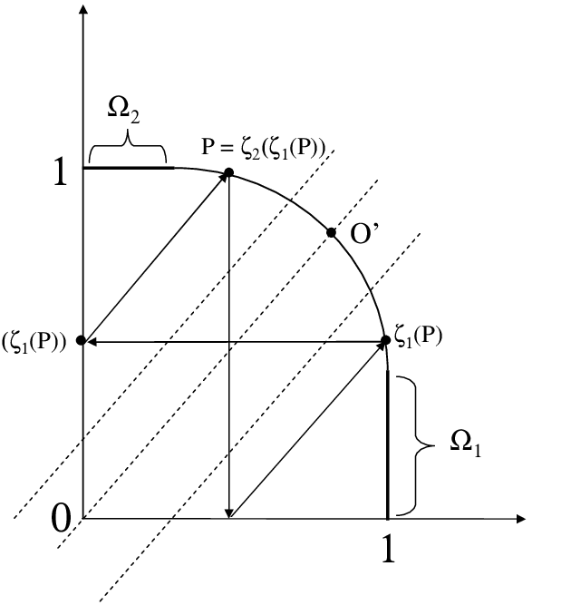
We construct a guided dynamical system on $\Gamma$ . For any point $p$ in $\overline{D}$ , define $\pi_{1}p$ to be the projection of $p$ onto the $x$ -axis and $\pi_{2}p$ to be the projection of $p$ onto the $y$ -axis. Through $p$ there is a line $\ell=\{p+(mt,nt):t\in\mathbb{R}\}$ . Let $\pi_{3}p$ to be the unique point of intersection of the line $\ell$ passing through $p$ and of $\Gamma$ . Note that $\pi_{1}$ , $\pi_{2}$ and $\pi_{3}$ project along characteristic lines of the operators $\partial y$ , $\partial x$ and $m\partial x+n\partial y$ , respectively. We now define two maps in $\Gamma$

\zeta_{1}=\pi_{3}\circ\pi_{1}\quad{\rm and}\quad\zeta_{2}=\pi_{3}\circ\pi_{2}\quad.

We introduce the guiding sets

\Omega_{1}=\{q\in\Gamma\,|\,\,(0,1)_{q}\in T_{q}(\Gamma)\}

and

\Omega_{2}=\{q\in\Gamma\,|\,\,(1,0)_{q}\in T_{q}(\Gamma)\}\quad.

In words: the set $\Omega_{1}$ is precisely the subset of $\Gamma$ consisting of points where the tangent line is parallel to the $y$ -axis, and a similar statement holds for $\Omega_{2}$ (see figure 4.3). It turns out that the dynamical properties of $(\Gamma,\zeta,\Omega)$ determine precisely the solvability of the homogeneous problem (4.2)-(4.3). Before anything else we must explain what we mean by “a solution to (4.2)-(4.3)”.

Definition 4.1.1.

A function $u\in C(\overline{D})$ is called a generalized solution to the problem (4.2)-(4.3) if

u\Big|_{\partial D}=g

and if for any $\varphi\in C_{0}^{\infty}(D)$

-\int_{D}u\,(m\partial_{x}+n\partial_{y})\partial_{x}\partial_{y}\,\varphi\,dxdy=0\quad.

It is convenient to reduce the boundary problem we are interested in to the problem studied in subsection 2.3.4. Define a map $\omega_{\Gamma}:\Gamma\rightarrow I:=[-m,n]$ by

\omega_{\Gamma}(x,y)=nx-my\,\,.

Define two maps $\delta_{1},\delta_{2}$ in $I$ by

\delta_{i}=\omega_{\Gamma}\circ\zeta_{i}\circ{\omega_{\Gamma}}^{-1}\,\,.

If we denote $\Lambda_{i}=\{t\in I\,|\,\delta_{i}^{\prime}(t)=0\}$ , then lemma 5 in [17] tells us that $(\Gamma,\zeta,\Omega)$ and $(I,\delta,\Lambda)$ are isomorphic as guided dynamical systems. By lemma 4 in that paper $(I,\delta,\Lambda)$ is a $\mathcal{P}$ -configuration. In that same paper it is shown that finding a generalized solution to problem (4.2)-(4.3) is equivalent to the problem of finding some function $f\in C^{2}(I)$ satisfying the following conditions:

	$\displaystyle f(t)-f(\delta_{1}(t))-f(\delta_{2}(t))$	$\displaystyle=$	$\displaystyle h(t)\quad,\quad t\in I$
	$\displaystyle f^{\prime}(0)$	$\displaystyle=$	$\displaystyle 0$

where $h$ is an arbitrary $C^{2}(I)$ function satisfying the boundary conditions $h(-m)=h(n)$ . Combining this reduction and theorems 2.3.5 and 1.3.4 we immediately obtain :

Theorem 4.1.2.

Let $D$ and $\Gamma$ be the domain and the curve described above. For any $g\in C^{2}(\Gamma)$ there exists a unique generalized solution $u\in C^{2}(\overline{D})$ of the problem (4.2)-(4.3) if and only if $(\Gamma,\zeta,\Omega)$ is $\Omega$ -minimal.

Remark 4.1.3.

It should be noted that in 1941 F. John obtained results²² 2 [6] tying the solvability of the Dirichlet problem for the wave equation with the dynamical behavior of some system on the boundary of a domain generated by the characteristics of the wave operator $\partial_{x}\partial_{y}$ .

4.2 Explicit conditions for solvability

Theorem 4.1.2 gives the intimate connection between the dynamical system generated on $\Gamma$ by the characteristic lines of the operators $\partial x$ , $\partial y$ and $m\partial_{x}+n\partial_{y}$ and the unique solvability of the second partly characteristic boundary value problem. But the condition in the theorem might seem rather vague. It would be very interesting to find a geometrical condition on $\Gamma$ that is necessary and sufficient for $(\Gamma,\zeta,\Omega)$ to be $\Omega$ -minimal, but, unfortunately, we have not been able to find such a condition. In this section we give explicit conditions that are sufficient for unique solvability. These conditions will allow us to “solve” problem (4.2)-(4.3) in domains that couldn’t be dealt with within the framework of the theory developed until now. In this section we stick with the notation of the previous section.

Before stating our results, let us review the results already known.

Definitions 4.2.1.

Let $\mathcal{O}=(p_{1},p_{2},\ldots p_{N})$ be an orbit

•

If all the points in $\mathcal{O}$ belong to $\Omega$ then $\mathcal{O}$ is called an $\Omega$ -guided orbit.
•

If $p_{1}=p_{N}$ then $\mathcal{O}$ is called a cycle.

We denote by $\mathcal{N}^{\Omega}_{\zeta}$ the set of all $\Omega$ -proper, $\Omega$ -guided cycles in $\Gamma$ . Also, we let $\Omega_{j}^{\prime}$ be the set of limit points of $\Omega_{j}$ , for $j=1,2$ . In [17] it is proved that if the following two conditions hold:

1: $\Gamma$ is transversal to the $x$ and $y$ axes at $A_{1}$ and $A_{2}$ ,
2: All possible pairs of points $p_{1}\in\Omega_{1}^{\prime}$ and $p_{2}\in\Omega_{2}^{\prime}$ are situated on $\Gamma$ in the order $A_{2},p_{1},p_{2},A_{1}$ ;

then problem (4.2)-(4.3) is uniquely solvable if and only if $\mathcal{N}^{\Omega}_{\zeta}=\emptyset$ . We do not know wether $\mathcal{N}^{\Omega}_{\zeta}=\emptyset$ is a sufficient condition for unique solvability when conditions 1 and 2 are not fulfilled³³ 3 Necessity remains, since an $\Omega$ -proper, $\Omega$ -guided cycle is an $(\Omega,\zeta)$ -invariant closed subset of $\Gamma$ . . Our main purpose in this section is to prove the solvability of the second partly characteristic boundary value problem in domains not satisfying conditions 1 and 2.

Proposition 4.2.2.

Assume that $A_{1}\notin\Omega$ , and assume that for any point $p\in\Omega_{1}$ there is an $\Omega$ -proper orbit

(p,p_{1},\ldots,p_{N})

such that

p_{N}\notin\bigcup_{k\geq 0}{\zeta_{1}}^{-k}(\Omega_{1})

that is, for no $k\geq 0$ the inclusion ${\zeta_{1}}^{k}(p_{N})\in\Omega_{1}$ is possible. Then for any $g\in C^{2}(\partial D)$ there exists a unique generalized solution $u\in C^{2}(\overline{D})$ to (4.2)-(4.3).

Proof.

Due to theorem 4.1.2, it is enough to prove that $(\Gamma,\zeta,\Omega)$ is $\Omega$ -minimal. By proposition 2.3.4 it is enough to prove that $(\Gamma,\zeta,\Omega)$ has an $\Omega$ -weak attractor not in $\Omega$ . We shall show that the point $A_{1}$ is the desired weak attractor.

First, note that for any $p\in\Gamma$ the sequence $(p,\zeta_{1}(p),\zeta_{1}^{2}(p),\ldots)$ converges to $A_{1}$ . Now for any point $p_{0}\in\Gamma$ , consider the longest $\Omega$ -proper orbit

(p_{0},\zeta_{1}(p_{0}),\zeta_{1}^{2}(p_{0}),\ldots)\,\,.

If this orbit is infinite, then it converges to $A_{1}$ by the above remark. If this orbit is finite, then there is some $N\geq 0$ such that $(p_{0},\zeta_{1}(p_{0}),\zeta_{1}^{2}(p_{0}),\ldots,\zeta_{1}^{N}(p_{0}))$ is $\Omega$ -proper but $\zeta_{1}^{N}(t_{0})\in\Omega_{1}$ . But by the assumption of the theorem there is an $\Omega$ -proper orbit $(\zeta_{1}^{N}(p_{0}),p_{1},\ldots,p_{M})$ such that $p_{M}\notin\bigcup_{k\geq 0}{\zeta_{1}}^{-k}(\Omega_{1})$ . Thus

(p_{0},\zeta_{1}(p_{0}),\zeta_{1}^{2}(p_{0}),\ldots,\zeta_{1}^{N}(p_{0}),p_{1},\ldots,p_{M},\zeta_{1}(p_{M}),\zeta_{1}^{2}(p_{M}),\zeta_{1}^{3}(p_{M}),\ldots)

is $\Omega$ -proper and converges to $A_{1}$ . ∎

Example 4.2.3.

Consider the domain in figure 4.4. Although $\Gamma$ does not satisfy neither of conditions 1 or 2 above, yet, by the above proposition, the boundary problem

	$\displaystyle(\partial_{x}+\partial_{y})\partial_{x}\partial_{y}u$	$\displaystyle=$	$\displaystyle 0\quad{\rm in}\quad D$
	$\displaystyle u$	$\displaystyle=$	$\displaystyle g\quad{\rm on}\quad\partial D$

has a unique generalized solution $u\in C^{2}(\overline{D})$ for any $g\in C^{2}(\partial D)$ .

The above example is not contained in the results that appeared up to now, but could have been obtained using the same techniques. The next proposition deals with a configuration that truly makes use of the methods and notions that we have introduced in this thesis.

Before we state our next proposition, let us make some further notation and remarks. There is some point $z_{0}\in[-1,1]$ such that $(\alpha_{1}(z_{0}),\alpha_{2}(z_{0}))=\zeta_{1}(A_{2})=\zeta_{2}(A_{1})$ . Denote $O^{\prime}=(\alpha_{1}(z_{0}),\alpha_{2}(z_{0}))$ . By the open segment $A_{2}O^{\prime}$ we shall mean the homeomorphic image of $[-1,z_{0})$ in $\Gamma$ . The open segment $O^{\prime}A_{1}$ is defined similarly.

Now let $(I,\delta,\Lambda)$ be the guided dynamical system defined in the discussion before theorem 4.1.2. The map $\delta_{1}\circ\delta_{2}:I\rightarrow I$ (and similarly, $\delta_{2}\circ\delta_{1}$ ) satisfies the inequality

\left(\delta_{1}\circ\delta_{2}\right)^{\prime}(t)=\delta_{2}^{\prime}(t)\cdot\delta_{1}^{\prime}(\delta_{2}(t))\leq 1

(4.4)

for all $t$ in $I$ . For all points $t$ not contained in $\Lambda$ , this map satisfies the stronger inequality

\left(\delta_{1}\circ\delta_{2}\right)^{\prime}(t)<1\,\,.

(4.5)

The following lemma shows the importance of conditions (4.4)-(4.5).

Lemma 4.2.4.

Let $I$ be a closed interval, and let $f:I\rightarrow I$ be a non-decreasing $C^{1}$ function satisfying $f^{\prime}\leq 1$ . Let $t_{0}\in I$ be a fixed point⁴⁴ 4 It is well known that every continuous function from an interval into itself has a fixed point. of $f$ . If $f^{\prime}(t_{0})<1$ then $t_{0}$ is the unique fixed point of $f$ and, moreover, for any $t\in I$ the sequence

(t,f(t),f^{2}(t),f^{3}(t),\ldots)

converges to $t_{0}$ .

Proof.

Assume, without loss of generality, that $t_{0}$ is an inner point of $I$ . Define a function $T:I\rightarrow I$ by $T(t)=t$ . We have that $f^{\prime}\leq T^{\prime}$ in $I$ . Let $t_{1}>t_{0}$ . Since $f^{\prime}(t_{0})<1=T^{\prime}(t_{0})$ , there is a neighborhood $U$ of $t_{0}$ such that $f^{\prime}(t)<T^{\prime}(t)$ for all $t\in U$ . Thus

f(t_{1})-f(t_{0})=\int_{t_{0}}^{t_{1}}f^{\prime}(t)\,dt<\int_{t_{0}}^{t_{1}}T^{\prime}(t)\,dt=t_{1}-t_{0}\,\,.

but $t_{0}$ is a fixed point of $f$ , thus

f(t_{1})<t_{1}\,\,.

(4.6)

As a consequence, no point $t_{1}$ greater than $t_{0}$ can be a fixed point of $f$ . On the other hand,

f(t_{1})\geq f(t_{0})=t_{0}

(4.7)

because $f$ is non-decreasing. The combination of (4.6) and (4.7) implies that the sequence

(t_{1},f(t_{1}),f^{2}(t_{1}),f^{3}(t_{1}),\ldots)

converges to some $t_{2}\geq t_{0}$ . Thus $t_{2}$ is a fixed point of $f$ , and using (4.6) again we conclude that $t_{2}=t_{0}$ . In a similar we may obtain the same results for $t_{1}<t_{0}$ . This completes the proof of the lemma. ∎

Now, assume that the map $\zeta_{1}\circ\zeta_{2}$ has a fixed point $p_{1}$ outside of $\Omega$ . This fixed point is mapped by the isomorphism⁵⁵ 5 See the discussion preceding theorem 4.1.2. $w_{\Gamma}$ to a fixed point $t_{1}\notin\Lambda$ of $\delta_{1}\circ\delta_{2}$ . By the discussion before the lemma,

\left(\delta_{1}\circ\delta_{2}\right)^{\prime}(t_{1})<1\,\,.

Using the lemma, we conclude that $t_{1}$ is an attractive fixed point of $\delta_{1}\circ\delta_{2}$ , and this translates to the fact that for any $p\in\Gamma$ , the sequence

(p,\zeta_{1}(\zeta_{2}(p)),\zeta_{1}(\zeta_{2}(\zeta_{1}(\zeta_{2}(p)))),\ldots)

converges to $p_{1}$ . The same discussion can also be made for fixed points of $\zeta_{2}\circ\zeta_{1}$ .

Proposition 4.2.5.

Assume that $\Omega_{1}$ is contained in the open segment $O^{\prime}A_{1}$ , and that $\Omega_{2}$ is contained in the open segment $A_{2}O^{\prime}$ . Then the problem (4.2)-(4.3) has a (unique) generalized solution $u\in C^{2}(\overline{D})$ for every $g\in C^{2}(\partial D)$ if and only if either $\zeta_{1}\circ\zeta_{2}$ or $\zeta_{2}\circ\zeta_{1}$ has a fixed point not in $\Omega$ .

Proof.

Assume that neither $\zeta_{1}\circ\zeta_{2}$ nor $\zeta_{2}\circ\zeta_{1}$ have fixed points outside $\Omega$ . Denote by $p_{1}$ a fixed point of $\zeta_{1}\circ\zeta_{2}$ lying in $\Omega$ . Because $p_{1}\in\overline{O^{\prime}A_{1}}$ , $p_{1}$ must be in $\Omega_{1}$ . Let $p_{2}=\zeta_{2}(p_{1})$ . Now,

\zeta_{2}(\zeta_{1}(\zeta_{2}(p_{1})))=\zeta_{2}(p_{1})\,\,,

so $p_{2}$ is a fixed point of $\zeta_{2}\circ\zeta_{1}$ . By assumption, $p_{2}\in\Omega$ , but because $p_{2}\in\overline{A_{2}O^{\prime}}$ , $p_{2}$ must be in $\Omega_{2}$ . Therefore, set $\{p_{1},p_{2}\}$ is a closed, $(\Omega,\zeta)$ -invariant set in $\Gamma$ ⁶⁶ 6 In other words, $\{p_{1},p_{2}\}$ is an $\Omega$ -proper, $\Omega$ -guided cycle.. As $(\Gamma,\zeta,\Omega)$ cannot be $\Omega$ -minimal, theorem 4.1.2 tells us that there are $g\in C^{2}(\partial D)$ for which there is no solution $u$ to (4.2)-(4.3).

Now assume, without loss of generality, that a fixed point $p_{1}$ of $\zeta_{1}\circ\zeta_{2}$ is not in $\Omega$ . It is enough to show that $p_{1}$ is an $\Omega$ -weak attractor. Let $p$ be a point in the closed segment $O^{\prime}A_{1}$ . As $\Omega_{2}$ is contained in the open segment $A_{2}O^{\prime}$ , the orbit $(p,\zeta_{2}(p))$ is $\Omega$ -proper. Now, $\zeta_{2}(p)$ is in the closed segment $A_{2}O^{\prime}$ , so $(p,\zeta_{2}(p),\zeta_{1}(\zeta_{2}(p)))$ is also an $\Omega$ -proper orbit. Continuing in this fashion, we get an $\Omega$ -proper orbit

(p,\zeta_{2}(p),\zeta_{1}(\zeta_{2}(p)),\zeta_{2}(\zeta_{1}(\zeta_{2}(p))),\ldots)

But this orbit contains the sub-sequence

(p,\zeta_{1}(\zeta_{2}(p)),\zeta_{1}(\zeta_{2}(\zeta_{1}(\zeta_{2}(p)))),\ldots)

which, as we have mentioned above, converges to $p_{1}$ . So for any $p$ in the closed segment $O^{\prime}A_{1}$ , we have $p_{1}\in\overline{\Omega{\rm-}OS(p)}$ . Now if $p$ is in the closed segment $A_{2}O^{\prime}$ , then $(p,\zeta_{1}(p))$ is $\Omega$ -proper and $\zeta_{1}(p)$ is now in the open segment $O^{\prime}A_{1}$ . So $p_{1}\in\overline{\Omega{\rm-}OS(\zeta_{1}(p))}$ which clearly implies that $p_{1}\in\overline{\Omega{\rm-}OS(p)}$ . We have established the fact that $p_{1}$ is an $\Omega$ -weak attractor, and the proof is completed by calling into action proposition 2.3.4 and theorem 4.1.2. ∎

Example 4.2.6.

The domain in figure 4.6 does not satisfy condition 1 nor condition 2, but the map $\zeta_{1}\circ\zeta_{2}$ has a fixed point $p\notin\Omega$ so by the above proposition the boundary value problem

	$\displaystyle(\partial_{x}+\partial_{y})\partial_{x}\partial_{y}u$	$\displaystyle=$	$\displaystyle 0\quad{\rm in}\quad D$
	$\displaystyle u$	$\displaystyle=$	$\displaystyle g\quad{\rm on}\quad\partial D$

has a unique generalized solution $u\in C^{2}(\overline{D})$ for any $g\in C^{2}(\partial D)$ .

Example 4.2.7.

Consider figure 4.6. The fixed points of $\zeta_{1}\circ\zeta_{2}$ and $\zeta_{2}\circ\zeta_{1}$ are in $\Omega$ , so by the above proposition there are functions $g\in C^{2}(\partial D)$ for which the boundary value problem

	$\displaystyle(\partial_{x}+\partial_{y})\partial_{x}\partial_{y}u$	$\displaystyle=$	$\displaystyle 0\quad{\rm in}\quad D$
	$\displaystyle u$	$\displaystyle=$	$\displaystyle g\quad{\rm on}\quad\partial D$

has no solution $u\in C^{2}(\overline{D})$ .

We are able to state the last proposition using the compact condition that Paneah used. Recall that $\mathcal{N}^{\Omega}_{\zeta}$ is the set of all $\Omega$ -proper, $\Omega$ -guided cycles in $(\Gamma,\zeta,\Omega)$ . Then we have

Corollary 4.2.8.

Under the assumptions of proposition 4.2.5, the problem (4.2)-(4.3) has a (unique) generalized solution $u\in C^{2}(\overline{D})$ for every $g\in C^{2}(\partial D)$ if and only if $\mathcal{N}^{\Omega}_{\zeta}=\emptyset$ .

Proof.

We have already mentioned that $\mathcal{N}^{\Omega}_{\zeta}=\emptyset$ is a necessary condition for unique solvability. Now if $\mathcal{N}^{\Omega}_{\zeta}=\emptyset$ , the above proof shows that for either $\zeta_{1}\circ\zeta_{2}$ or $\zeta_{2}\circ\zeta_{1}$ there has to be a fixed point $p\notin\Omega$ , thus the above proposition implies the assertion of the corollary. ∎

Following the idea of the last proposition, we may obtain sufficient conditions for solvability in terms of the fixed points of $\zeta_{i_{1}}\circ\zeta_{i_{2}}\circ\cdots\circ\zeta_{i_{N}}$ , for an arbitrary multi-index $(i_{1},i_{2},\ldots,i_{N})$ . But we shall not write down such theorems. It is the author’s belief that the best kind of progress will be made by finding a simple and analytical (or geometrical) necessary and sufficient condition for the guided dynamical system $(\Gamma,\zeta,\Omega)$ to be minimal. We conclude this thesis with a conjecture in this direction. We state this conjecture in terms of the second partly characteristic boundary value problem, although it may also be viewed as a conjecture regarding the minimality of a $\mathcal{P}$ -configuration.

Conjecture 4.2.9.

The boundary value problem (4.2)-(4.3) is uniquely solvable if and only if $\mathcal{N}^{\Omega}_{\zeta}=\emptyset$ .

Chapter 5 Late introduction

The main theme of this thesis is the use of guided dynamical systems in problems in functional equations and in partial differential equations. Most of the problems we deal with were first studied by Paneah in the papers cited in the text, and originated from the problem dealt with in [12]. In this introduction we give a brief overview of the results in this thesis and survey related known results.

5.1 Chapter 1

Guided dynamical systems are a generalization of dynamical systems with several generators. A guided dynamical system is simply a dynamical system in which each of the generating maps acts only on a subset of the space. The first guided dynamical systems appeared in [13] and [14]. In these papers the space was an interval or a curve, and on it acted two generating maps.

Chapter 1 is a first step in the development of a general theory of guided dynamical systems. We develop only the parts of the theory that are used in other parts of this thesis¹¹ 1 Theorem 1.2.8 is exception to this rule. It was proved because of its beauty, not its usefulness.. It is the author’s belief that there is much work left to be done in the general theory of guided dynamical systems, which appears both potentially applicable to other parts of Mathematics and interesting in itself.

In section 1.1 we set the notation for (non-guided) discrete dynamical systems, define the basic terms and obtain the first (original) result in this work - proposition 1.1.4. The exposition is influenced by two main approaches: the first that of Paneah, which is non-standard but convenient for our uses, and the second is the approach of B. Hasselblat and A. Katok [7]. We found it necessary to introduce the term weak attractor since, on the one hand, the notion this term represents plays a key role in the theory we develop and, on the other hand, such a notion has not been given a name in the literature.

Sections 1.2 and 1.3 deal with generalizing well-known definitions and results from the theory of discrete dynamical systems to guided dynamical systems. A particular case of lemma 1.3.3 was proved in lemma 5 of [17]. In that paper there was an isomorphism of guided dynamical systems between to specific guided dynamical systems - one on an interval and one on a curve.

5.2 Chapter 2

This chapter is devoted to uniqueness and solvability of functional equations that have the form

f(x)-\sum_{i=1}^{N}a_{i}(x)f(\delta_{i}(x))=h(x)\quad,\,\,x\in X\,\,.

(5.1)

Here the functions $a_{i}$ , $\delta_{i}$ and $h$ are given, and $f$ is an unknown function on $X$ . In [14] Paneah studies this equation where $X$ was an interval and the $\delta_{i}$ ’s were non-decreasing maps satisfying some conditions.

In subsection 2.1.1 we generalize the first parts of theorems 1 and 2 in [14] in a few directions. Theorem 2 from [14] (the maximum principle), originally stated for continuous functions, is generalized to semi-continuous functions (lemma 2.1.2). Theorem 2 (uniqueness of solutions), originally stated for scalar valued functions, is generalized to vector valued functions (2.1.6). In both cases our results hold for (at least) a general compact metric space $X$ . Our sufficient condition for uniqueness up to an additive constant is given in terms of the existence of a $\Lambda$ -weak attractor.

Subsection 2.1.2 deals with uniqueness of continuously differentiable solutions of (5.1) with $N=2$ , $a_{1}\equiv a_{2}\equiv 1$ and $X$ a subset of $\mathbb{R}^{n}$ . Theorems 2.1.8 and 2.1.11 are the main results of this subsection. Such results were obtained by Paneah in [18] for classes of functions defined on an interval and differentiable either at the origin or on the entire interval - depending on the behavior of the $\delta_{i}$ ’s. As above, our sufficient condition for uniqueness up to an multiplicative constant is given in terms of the existence of a $\Lambda$ -weak attractor.

The main results in section 2.2 is theorem 2.2.1. This theorem is a generalization of the second part of theorem 3 in [13] (regarding unique solvability of equation 5.1) originally stated for maps on an interval with an attractor in the boundary of the interval, to general guided dynamical systems with some weak attractor. We give a proof that is based on the proof in [13], adding a few details. Our sufficient condition for unique-solvability is given in terms of the existence of a $\Lambda$ -weak attractor.

In section 2.3.4 we treat the problem of existence and uniqueness of $C^{2}$ solutions $f$ to the problem

	$\displaystyle f(t)-\sum_{i=1}^{N}f(\delta_{i}(t))$	$\displaystyle=$	$\displaystyle h(t)\quad,\quad t\in I$		(5.2)
	$\displaystyle f^{\prime}(c)$	$\displaystyle=$	$\displaystyle\mu\quad,$		(5.3)

where $I=[a,b]$ is an interval, $h\in C^{2}(I)$ is given and the maps $\delta_{i}$ , $i=1,\ldots,N$ satisfy what we call a generalized $\mathcal{P}$ -configuration²² 2 $\mathcal{P}$ -configurations were introduced by Paneah in the papers cited here.. To be precise, we give a necessary and sufficient condition for the existence and uniqueness of solution to (5.2)-(5.3). This necessary and sufficient condition is given in terms of a dynamical property of the guided dynamical system generated in $I$ by the maps $\delta_{i}$ , $i=1,\ldots N$ . Theorem 2.3.5 states that it is the $\Lambda$ -minimality of this dynamical system that is necessary and sufficient for the unique solvability of the above problem. This is an improvement on theorem 9 from [14] for two reasons. First, the passage from $2$ to $N$ maps is not completely trivial. Second, we give a necessary and sufficient condition, whereas until now a necessary and sufficient condition for unique solvability was known only under some additional conditions. Another interesting new result in this section is proposition 2.3.4, which states that for a generalized $\mathcal{P}$ -configuration the existence of a $\Lambda$ -weak attractor (in some set) is equivalent to $\Lambda$ -minimality.

5.3 Chapter 3

In chapter 3 we give two results regarding overdeterminedness of functional equations. Details about this subject are given in the beginning of that chapter. In theorem 3.1.1 we prove that if a continuous function $f:[0,1]\rightarrow\mathbb{R}$ satisfies Cauchy’s functional equation

f(x+y)=f(x)+f(y)

(5.4)

on part of the boundary of the square ${\bf K}=\{(x,y):|x|+|y|\leq 1\}$ then $f(z)=\lambda z$ . This result is weaker in some sense than a known result of Lackovich, who showed in [11] that if $f:[0,\infty)\rightarrow\mathbb{R}$ is measurable and satisfies Cauchy’s equation on the line $\{(at,bt)|t\in\mathbb{R}\}$ where $\log_{a}b\notin\mathbb{Q}$ , then $f(z)=\lambda z$ . Our contributions are that we have shown that the continuous solutions of equation (5.4) are determined on the boundary of ${\bf K}$ , and also that we give a very simple proof based on dynamical systems³³ 3 Lackovich’ proof relied on the Krein-Milman theorem, whereas our proof uses quite elementary analysis. One may also compare our results to theorem 1 in [18], where it is shown that the $C^{1}$ solutions of (5.4) are determined on even a smaller part of the boundary of ${\bf K}$ .

Theorem 3.2.2 can be viewed either as a uniqueness theorem or as an overdeterminedness theorem. As a uniqueness theorem, it is very similar to Aczél’s theorem 3.2.1, just the conditions are slightly different and the proof is completely different. As an overdeterminedness theorem, it is probably the first of its kind.

5.4 Chapter 4

In [17] Paneah reduces the so-called “second partly characteristic” third order strictly hyperbolic boundary value problem to a Cauchy type functional equation. This reduction, together with theorems 1.3.4 and 2.3.5, immediately imply theorem 4.1.2. This theorem gives the precise connection between the dynamics in the boundary of the problem and the solvability of that problem.

Propositions 4.2.2 and 4.2.5 give sufficient conditions for solvability in domains for which there was no previous result.

Bibliography

[1] J. Aczél. On Applications and Theory of Functional Equations. Birkhauser Boston, 1966.
[2] J. Aczél. On applications and theory of functional equations. Elemente der Mathematik Vom Hoheren Standpunkt Ans. Birkhauser Verlag, 1969.
[3] J. Aczél and J. Dhombres. Functional Equations in Several Variables. Cambridge University Press, 1989.
[4] S. Ardazi, V. Kharash, E. Mamane, and N. Zoabi. Cauchy’s and pexider’s functional equations in restricted domains, 2004. in SciTech 2004, Students’ Scientific Reports, Technion International Youth Summer Research Program.
[5] K. Hoffman and R. A. Kunze. Linear Algebra. Prentice Hall, 2nd edition, 1971.
[6] F. John. The dirichlet problem for a hyperbolic equation. Amer. J. Math., 63:141–154, 1941.
[7] A. Katok and B. Hasselblatt. Introduction to the Modern Theory of Dynamical Systems. Cambridge University Press, 1995.
[8] M. Kuczma. Functional equations in a single variable. PWN – Polish Scientific Publishers, 1968.
[9] M. Kuczma. Fuctional equations on restricted domains. Aequationes Mathematicae, 18:1–34, 1978.
[10] M. Kuczma, B. Choczewski, and R. Ger. Iterative functional equations. Encyclopedis of mathematics and its application. Cambridge University Press, 1990.
[11] M. Laczkovich. Non-negative measurable solutions of a difference equation. J. London Math. Soc., 34(2):139–147, 1986.
[12] B. Paneah. On a problem in integral geometry connected to the dirichlet problem for hyperbolic equations. International Mathematics Research Notes, 5:213–222, 1997.
[13] B. Paneah. Noncommutative dynamical systems with two generators and their applications in analysis. Discrete and Continuous Dynamical Systems, 9(6), 2003.
[14] B. Paneah. On solvability of functional equations relating to dynamical systems with two generators. Functional Analysis and Its Applications, 37(1), 2003.
[15] B. Paneah. Boundary problems for higher order hyperbolic differential equations in bounded domains. Russian Journal of Mathematical Physics, 11(4):311–330, 2004.
[16] B. Paneah. Dynamic methods in the general theory of cauchy type functional equations. Contemporary Mathematics, 364, 2004.
[17] B. Paneah. Dynamical approach to some problems in integral geometry. Trans. Amer. Math. Soc., 356:2757–2780, 2004.
[18] B. Paneah. On the overdeterminedness of some functional equations. Discrete and Continuous Dynamical Systems, 10(1,2), 2004.
[19] M. Sablik. Note on a cauchy conditional equation. Radovi Matematicki, 1:241–245, 1985.
[20] M. Sablik. Some remarks on cauchy equation on a curve. Demonstration Mathematica, 23(2):477–490, 1990.
[21] E. W. Weisstein. Mathworld. http://mathworld.wolfram.com/.
[22] E. Zeidler. Nonlinear Functional Analysis and its Applications, volume 1. Springer Verlag, 1986.

Chapter 1 Discrete guided dynamical systems with several generators

1.1 Dynamical systems with several generators

Definitions 1.1.1.

Remark 1.1.2.

Example 1.1.3.

Proposition 1.1.4.

Proof.

Lemma 1.1.5.

Proof.

Definitions 1.1.6.

1.2 Guided dynamical systems

Definition 1.2.1.

Definition 1.2.2.

Remark 1.2.3.

Meta-Definition 1.2.4.

Example 1.2.5.

Definition 1.2.6.

Lemma 1.2.7.

Proof.

Theorem 1.2.8.

Proof.

Proposition 1.2.9.

Proof.

1.3 Isomorphism of guided dynamical systems

Definition 1.3.1.

Definition 1.3.2.

Lemma 1.3.3.

Proof.

Theorem 1.3.4.

Proof.

Chapter 2 Some results in functional equations

2.1 The Maximum principle for functional equations

2.1.1 The maximum principle

Definition 2.1.1.

Lemma 2.1.2.

Proof.

Corollary 2.1.3.

Proof.

Lemma 2.1.4.

Proof.

Example 2.1.5.

Theorem 2.1.6.

Proof.

Corollary 2.1.7.

2.1.2 An application to Cauchy type functional equations

Theorem 2.1.8.

Proof.

Example 2.1.9.

Example 2.1.10.

Theorem 2.1.11.

Proof.

2.2 Unique solvability

Theorem 2.2.1.

Remark 2.2.2.

Proof.

Lemma 2.2.3.

Proof.

Lemma 2.2.4.

Proof.

Lemma 2.2.5.

Proof.

Lemma 2.2.6.

Proof.

2.3 The initial value problem for a 𝒫\mathcal{P}-configuration

2.3.1 Definition of a 𝒫\mathcal{P}-configuration

2.3.2 Generalized 𝒫\mathcal{P}-configuration

2.3.3 Some preliminary results in functional analysis and preparations

Lemma 2.3.1.

Proof.

2.3.4 The initial value problem

Theorem 2.3.2.

Proof.

Remark 2.3.3.

Proposition 2.3.4.

Theorem 2.3.5.

Remark 2.3.6.

Proof.

Chapter 3 Overdeterminedness of functional equations

3.1 Overdeterminedness of Cauchy’s functional equation

Theorem 3.1.1.

2.3 The initial value problem for a $\mathcal{P}$ -configuration

2.3.1 Definition of a $\mathcal{P}$ -configuration

2.3.2 Generalized $\mathcal{P}$ -configuration