Multiplicity-free Schubert calculus

Let $Gr(\ell,{\mathbb{C}}^{n})$ denote the Grassmannian of $\ell$-dimensional subspaces in ${\mathbb{C}}^{n}$. The cohomology ring ${\rm H}^{\star}(Gr(\ell,{\mathbb{C}}^{n}),{\mathbb{Z}})$ has an additive basis of Schubert classes $\sigma_{\lambda}$, indexed by Young diagrams $\lambda=(\lambda_{1}\geq\lambda_{2}\geq\ldots\geq\lambda_{\ell}\geq 0)$ contained in the $\ell\times k$ rectangle where $k=n-\ell$ (we denote this by $\lambda\subseteq\ell\times k$). The product of two Schubert classes in ${\rm H}^{\star}(Gr(\ell,{\mathbb{C}}^{n}),{\mathbb{Z}})$ is given by

where $c_{\lambda,\mu}^{\nu}$ is the classical Littlewood-Richardson coefficient (see, e.g., [3, 7]).

The expansion (1) is multiplicity-free if $c_{\lambda,\mu}^{\nu}\in\{0,1\}$ for all $\nu\subseteq\ell\times k$. In this paper, we give a nonrecursive, combinatorial answer to the following question of W. Fulton:

Famously, Littlewood-Richardson coefficients also arise as decomposition multiplicities of the tensor product $V^{\lambda}\otimes V^{\mu}=\bigoplus_{\nu}(V^{\nu})^{\oplus c_{\lambda,\mu}^{\nu}}$ of irreducible polynomial representations of $GL(\ell)$. Earlier, J. Stembridge [9] solved the analogous question in this context; the above question was motivated by this work. (The $GL(\ell)$ problem may be regarded as the special case in the “$k\to\infty$ limit” of Fulton’s question; Stembridge’s classification is expressed inside our solution below.)

For partitions $\lambda,\mu\subseteq\ell\times k$, place $\lambda$ against the upper left corner of the rectangle. Then rotate $\mu$ $180$ degrees and place it in the lower right corner. We refer to ${\rm rotate}(\mu)$ as the resulting subshape of $\ell\times k$. The boxes of these shapes refer to their configuration inside $\ell\times k$.

A boring reason for multiplicity-freeness is that $\lambda\cap{\rm rotate}(\mu)\neq\emptyset$, since the (intersection) product $\sigma_{\lambda}\cdot\sigma_{\mu}$ is merely zero. Geometrically, this reflects the fact that the Richardson variety $X_{\lambda}^{\mu}=X_{\lambda}(F_{\bullet})\cap X_{\mu}(F_{\bullet}^{{\rm opp}})$ is empty. This variety is the scheme-theoretic intersection of Schubert varieties indexed by $\lambda$ and $\mu$; these Schubert varieties are in general position when defined with respect to opposite complete flags $F_{\bullet}$ and $F_{\bullet}^{\rm opp}$.

Nevertheless, our main idea is to apply a simple extension of this classic geometric condition. Define a Richardson quadruple to be the datum $(\lambda,\mu,\ell\times k)$ where $\lambda\cap{\rm rotate}(\mu)=\emptyset$. If $\lambda\cup{\rm rotate}(\mu)$ does not contain a full $\ell$-column or $k$-row, call this Richardson quadruple basic. Otherwise, after removing all full columns and/or rows, we obtain a Richardson quadruple ${\widetilde{\mathfrak{R}}}=({\widetilde{\lambda}},{\widetilde{\mu}},{\widetilde{\ell}}\times{\widetilde{k}})$ for smaller partitions ${\widetilde{\lambda}},{\widetilde{\mu}}\subseteq{\widetilde{\ell}}\times{\widetilde{k}}$. This latter quadruple is basic, and we call it the basic demolition of ${\mathfrak{R}}$.

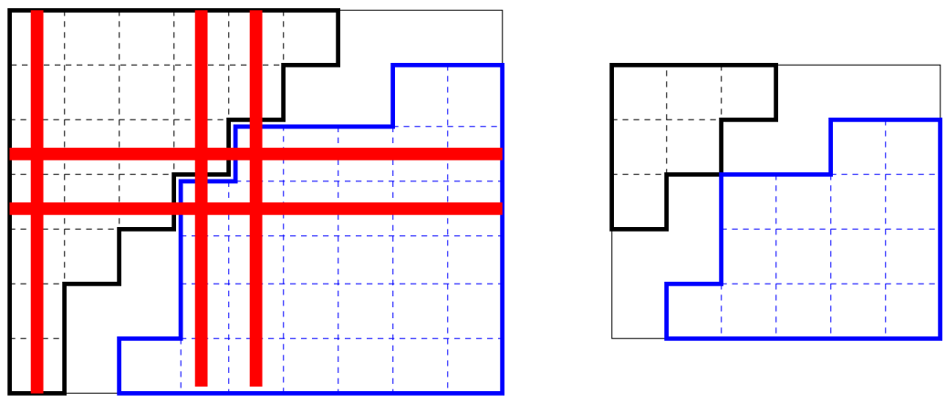
Conceptually, this combinatorics is inspired by a geometric comparison of Richardson varieties, $X_{\lambda}^{\mu}\subseteq Gr(\ell,{\mathbb{C}}^{\ell+k})$ and $X_{\widetilde{\lambda}}^{\widetilde{\mu}}\subseteq Gr({\widetilde{\ell}},{\mathbb{C}}^{{\widetilde{\ell}}+{\widetilde{k}}})$.

In order to state our main result, we need a little more notation and terminology, some nonstandard. A rectangle is a Young shape with exactly one distinct part size. A fat hook is a shape whose partition $\lambda$ has two distinct part sizes. Furthermore, $\lambda\subseteq\ell\times k$ naturally defines a lattice path from the southwest to the northeast corner points of the rectangle. A segment of this lattice path is a maximal consecutive sequence of north or east steps. The shortness of this lattice path is the length of its shortest segment. Lastly, a multiplicity-free Richardson quadruple is a Richardson quadruple such that the corresponding intersection product $\sigma_{\lambda}\cdot\sigma_{\mu}$ is multiplicity-free.

We are now ready to state our main result:

We remark that once the idea of basic demolitions is found, the solution to Fulton’s question becomes relatively straightforward, by exploiting [9, Theorem 3.1]; in the basic case, our classification is the same as Stembridge’s classification, although the proof requires further combinatorial analysis. However, as is often the case in combinatorics (and we believe here), the central difficulty of a problem often turns on precisely such an observation. In fact, after formulating this technique for this work, we found it to be crucial (in a more general form) for our arguments in [12].

Investigation of multiplicity-freeness in geometry and representation theory is of interest, see, e.g., [2, 9, 10] and the references therein.

In relation to the first of these papers cited, this report may be viewed as part of“multiplicity-free algebraic geometry”. By this term we mean the study of algebraic subvarieties $Y\subseteq X$ that have “the smallest invariants” according to the decomposition of their class into a predetermined linear basis of the Chow ring $A^{\star}(X)$. (In our case, the class of a Richardson variety decomposed into Schubert classes for the Grassmannian.)

A feature of our methods is that they extend naturally to other (classical) Lie types. In future work, we plan to study multiplicity-free Schubert calculus on cominuscule flag manifolds, a natural generalization of “Grassmannian”, with the following goal:

For the main interesting cases of Lagrangian and even orthogonal Grassmannians, the Schubert calculus is determined by the “shifted tableaux” combinatorics of Schur $P,Q$ polynomials [8, 5, 6]. Briefly, partitions with distinct parts contained in the staircase $\rho_{n}=(n,n-1,\ldots,3,2,1)$ index the Schubert classes. There is a standard simultaneous placement of shifted shapes $\lambda$ and $\mu$ into the shifted staircase $\rho_{n}$. When the shapes overlap, the product of their Schubert classes is zero. Otherwise, whenever there is a full $i$th column and $i+1$th row, the situation is a non basic Richardson triple. Removal of all such hooks is a basic Richardson triple.

This allows us to prove multiplicity-free characterizations (omitted here) with similar arguments to those found below. Results of C. Bessenrodt [1] can replace the role of [9]. (She studies the problem of multiplicity-freeness of Schur $P$ polynomials, in connection to projective outer products of spin characters.)

Finally, after a version of this paper was made available [11], C. Gutschwager [4] answered the question of determining multiplicity-free skew characters. As is explained there, this problem is equivalent to Fulton’s question.

We use a standard formulation of the Littlewood-Richardson rule: $c_{\lambda,\mu}^{\nu}$ counts the number of semistandard fillings of the skew-shape $\nu/\lambda$ of content $\mu$ such that the right to left, top to bottom reading word $w_{1}w_{2}\cdots w_{|\mu|}$ is a ballot sequence, i.e., the number of appearances of “$i$” in $w_{1}w_{2}\cdots w_{j}$ is at most the number of appearances of “$i-1$”, for $i\geq 2$ and $1\leq j\leq|\mu|$. We call these LR fillings.

We say a row or column of $\ell\times k$ is empty if it neither contains a box of $\lambda$ nor $\mu$. The following emptiness demolition is a simple application of the Littlewood-Richardson rule:

The following lemma explicates the demolition technique from the statement of the main theorem:

We use the following demolition technique throughout the proof of the main theorem. Suppose that ${\mathfrak{R}}$ contains a row or column of $\ell\times k$ containing boxes of $\lambda$, or alternatively ${\rm rotate}(\mu)$ but not both. Then define a Stembridge demolition to be the Richardson quadruple ${\overline{\mathfrak{R}}}=({\overline{\lambda}},{\overline{\mu}},{\overline{\ell}}\times{\overline{k}})$ corresponding to (sequentially) removing such rows or columns. (We emphasize that this differs from a basic demolition, which applies when a row or column contains only boxes of (possibly both) $\lambda$ and/or $\mu$.)

Stembridge demolitions are useful in one direction:

We find it useful to give an “inverse” formulatation of Theorem 1, i.e., in terms of when multiplicity appears:

This formulation is useful for induction on $\ell,k\geq 1$. For this, we are interested in the situations where a Stembridge demolition takes a basic ${\mathfrak{R}}$ satisfying (I’), (II’), (III’) or (IV’) of Theorem 1’ to a basic ${\overline{\mathfrak{R}}}$ that falls into the same case. We call these inductive Stembridge demolitions.

It is also possible to combine Stembridge and basic demolitions in inductive arguments, so long as we start and end in the same case (I’)-(IV’).

Let $\lambda,\mu$ have at least two distinct nonzero part sizes. By Proposition 1, one of its scenarios (a), (b) or (c) occurs. We induct if (a) happens.

Thus consider (b). Let $\mu=(b,1^{a})$ be a hook. Let $r$ be the smallest index such that $\lambda_{r}<\lambda_{1}$. Let $s$ be the smallest index such that $\lambda_{s}<\lambda_{r}$.

For the first filling, add a horizontal strip of boxes (i.e., no two in the same column) of size $b$ with each box labeled “1” such that:

• •

  at least one box appears in the first row, and in the $r$th row; and

• •

  the maximal possible number of boxes is not placed in row $s$ (so possibly no boxes occur there)

(Note that by basicness, $b<k$ and $\lambda_{1}^{\prime}<\ell$, so such a horizontal strip exists.) Now add $a$ boxes, no two in the same row, with a box at the right-hand end of all rows 2 through $a+2$, except row $r$. Label the box in row $i$ with “$i$” if $i<r$, and with “$i-1$” if $i>r$. This clearly gives a LR filling of a skew shape $\nu/\lambda$ with content $\mu$, as desired.

We modify the above to obtain a second LR filling: replace the rightmost “1” in row $r$ with an “$r$”. The column below the leftmost “1” in row $r$ consists of boxes labeled by “$r$” to “$s-2$”. Increase all of these labels by 1. Finally, replace the box labeled “$s-1$” in row $s$ by a “1”.

Now we turn to (c). Assume without loss of generality that ${\mathfrak{R}}$ is well-ordered. The example given in Figure 3 provides a running example.

To describe our LR fillings, think of the boxes of ${\rm rotate}(\mu)$ as movable tiles, labeled by their row number in $\mu$ (i.e., by $\ell-{\tt row}(\cdot)+1$).

Remove the tiles in the columns below $X$ and $Y$ (including $X$ and $Y$) and set them aside. Shift all the remaining tiles of ${\rm rotate}(\mu)$ one square to the left. Note that since ${\mathfrak{R}}$ is basic, the tiles still don’t overlap $\lambda$.

Using only columns $k-\mu_{1}$ to $k-1$, move the $\mu_{1}-2$ remaining columns of tiles (possibly left or right, but maintaining their relative order) so that the columns below $A$ and $B$ are empty.²² 2 Depending on the exact well-ordered configuration of $A,B,X$ and $Y$, there can be choice, but these all give the same end result. To be precise, we just insist that the same columns be used for both fillings described. Next slide these columns up so they are immediately below (the lattice path defined by) $\lambda$, and reverse the order of the tiles in each column. The only worry in this last step is that there might not be enough room to fit each column. It is straightforward to check that this cannot happen, because of the well-ordered assumption.

Let $a=\ell-{\tt row}(A)$ and $b=\ell-{\tt row}(B)$ count the number of boxes strictly below $A$ and $B$ respectively. Also, let $x=\ell-{\tt row}(X)+1$, $y=\ell-{\tt row}(Y)+1$ be the number of boxes in ${\rm rotate}(\mu)$ weakly below $X$ and $Y$. The tiles that we set aside consist of two copies of $1$ to $x$, together with one copy of $x+1$ to $y$. We wish to use these to fill the columns below $A$ and $B$ and the rightmost column.

For our first filling, put 1 in the rightmost column. Put 2 to $y-(a-x)$ in the column below $B$, and put $1$ to $x$ followed by $y-(a-x)+1$ to $y$ in the column below $A$. There is space to do this: under $A$ we use precisely $a$ labels, while under $B$ we use fewer than $b$ elements, precisely because of well-orderedness (4).

By construction, the associated word is a ballot sequence, because this is true for the word coming from the columns of labels we’ve inserted not below $A$ and $B$. (To each “$i$”, there is an “$i-1$” north of it in its column, which appears first in the reading word.) This property is clearly maintained after adding the three special columns. The only complaint is that this filling may not yet describe a skew-shape. We fix this by sliding tiles to the left (in the same row) as necessary. This doesn’t alter the reading word. Lastly, it is straightforward to verify that the filling is semistandard.

The second LR filling is similar: put $1$ in the rightmost column, $1$ to $y-(a-x)-1$ in the column below $B$, and $2$ to $x$ followed by $y-(a-x)$ to $y$ in the column below $A$. One also checks this satisfies the necessary conditions, and leads to an LR filling of the same shape as the first filling (even before the final left justificiation).

Let $\lambda$ have at least three part sizes and $\mu$ be a rectangle of shortness at least two. Thus, $\mu=(g^{h})$ where $2\leq g\leq k-2$ and $2\leq h\leq\ell-2$.

If $g$ or $h$ equals 2; by conjugation, we may assume that $h=2$. Note that the basicness assumption together with the fact that $\lambda$ contains at least three distinct parts, implies one can add to $\lambda$ a horizontal strip of length $g+2$ which uses (at least) four different rows. Call the rightmost boxes of these four rows $B_{1},B_{2},B_{3}$ and $B_{4}$ where ${\tt row}(B_{i})<{\tt row}(B_{j})$ when $i<j$.

If $\lambda$ does not extend to the $(\ell-1)$th row, then this horizontal strip can be done in any way possible; otherwise some extra care has to be made. In this latter situation, by inductive Stembridge reductions (removing the first few columns), we may assume that $\lambda$ has at least one column reaching the $(\ell-1)$ th row. Thus, choose our horizontal strip to include a (single) box in row $\ell$, and make that box $B_{4}$.

In either case, label the other $g-2$ boxes with “1”s. Place $g-2$ boxes labeled “2” under these boxes we have just labeled. These boxes give a skew shape $\nu/\lambda$ after sliding the boxes along each row to the left against the lattice path defined by $\lambda$. See Figure 6 below.

One LR filling of $\nu/\lambda$ is given by $B_{1}=B_{2}=1$, $B_{3}=B_{4}=2$; another is given by $B_{1}=B_{3}=1$, $B_{2}=B_{4}=2$. Thus, the result holds if $g$ or $h$ equals 2.

Now assume that $\mu=(g^{h})$ where $g,h\geq 3$. After applying inductive Stembridge demolitions one can assume (after conjugating) that $\lambda=(k-1,2^{a},1^{\ell-a-2})$, for some $a>0$. Proof: applying inductive Stembridge demolitions to rows and columns of $\lambda$ we can reduce to the case that $\lambda$ has exactly three part sizes. If neither the bottom row nor the rightmost column of $\lambda$ can be removed by an inductive Stembridge reduction, $\lambda$ must extend all the way to the $(k-1)$th column and $(\ell-1)$th row. Further inductive Stembridge demolitions to the first few columns/rows of $\lambda$ imply that $\lambda=(k-1,b^{a},1^{\ell-a-2})$. Finally, inductive Stembridge demolitions to columns $2$ through $b$, or rows $2$ through $a$ (depending on the position of $\mu$) allows us to deduce $b=2$ or $a=2$. Conjugating we may assume the former.

If $a+h+1>\ell$ then the Stembridge demolition obtained by removing the third column is clearly inductive if $g<k-3$. So we may assume that $g=k-3$. But then we can still Stembridge reduce by removing the third column. The result is non-basic (and thus not inductive). But removing the full rows that result gives us a smaller case of (II’), so we can still induct nonetheless.

Thus suppose $a+h+1\leq\ell$. We have an inductive Stembridge demolition by removing the third column unless $g=k-2$. Then removing the second row is an inductive Stembridge demolition unless $a=1$.

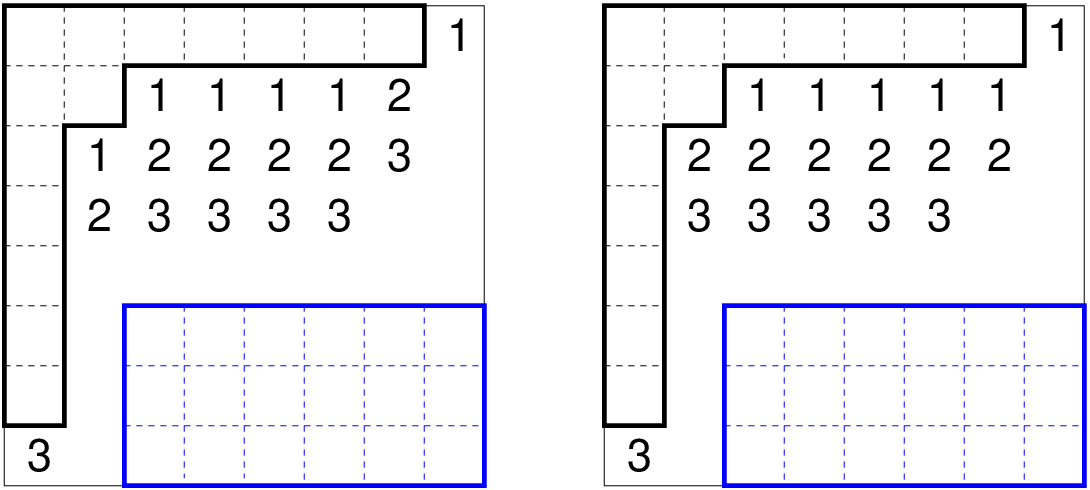
Summarizing we’ve reduced to the case that $\lambda=(k-1,2,1^{\ell-3})$ and $\mu=((k-2)^{h})$. Here is the first LR filling of a skew shape $\nu/\lambda$:

Let $\lambda=(c^{d},a^{b})$ be a fat hook of shortness at least 2 and let $\mu$ be a rectangle of shortness at least 3. Thus, $\mu=(g^{h})$ where $3\leq g\leq k-3$ and $3\leq h\leq\ell-3$.

Note that Lemma 1 implies that if $g>k-a$ then we can use emptiness demolitions and basic demolitions to obtain a basic situation that also lies in case (III’), so that we can conclude by induction. Similarly, we may assume from now on that $h<\ell-d$, since a similar argument holds if $h>\ell-d$, and since the $h=\ell-d$ reduces to the $g=k-a$ case handled below, after conjugation.

Next suppose $g=k-a-1$ (we’ll deal with $g=k-a$ after this). If moreover $3\leq h\leq b$, we have a filling $F_{h}$ of a skew shape $\nu/\lambda$ with content $\mu=(g^{h})$:

Our assumptions ensure that the insertion of columns gives rise to a skew-shape automatically. It is also easy to see that the corresponding reading word is a ballot sequence. Finally, when checking that the semistandard conditions hold, the only worry is between columns $c$ and $c+1$. But notice that by the assumption that all segments of the lattice path defined by $\lambda$ are of length at least $2$, the first comparison (in row $d+1>2$) is between a “$2$” in column $c$ and “$d+1$” in column $c+1$ is satisfactory. Since the labels in both columns increment by $1$ as we go down, all desired inequalities between these two columns are satisfied. The second filling $G_{h}$ is obtained by interchanging the bottom-most entries of columns $c-1$ and $c$. It is easy to see that this is also a LR filling. In the remaining cases, we invite the reader to consider how the fillings from the example above are adjusted.

If $h=b+1$, then we apply the instructions above, but when we place the entries in the columns as instructed, we see that we do not obtain a skew shape. However, we do obtain a skew shape if we push filled boxes to the left. Call the resulting fillings $F_{h+1}$ and $G_{h+1}$. It is easy to verify that they are again LR fillings of the same shape, of content $\mu$.

If $h>b+1$, define $F_{h}$ and $G_{h}$ by taking $F_{b+1}$ and $G_{b+1}$ and then adding $b+2,\dots,h$ onto the first $g$ columns. (Note that since $h<\ell-d$, there is always sufficient room to do this.) Now $F_{h}$ and $G_{h}$ clearly serve our purpose.

Next, when $g=k-a$, note that $a\geq 3$, so we can apply the same procedures as above, except we move the first two columns labeled with “$h-1,h$” and “$h$” to columns 2 and 3, and insert into column 1 the labels “$1,\ldots,h$”.

Finally, consider what happens when $g<k-a-1$. If we assume further that $h\leq b$, then simply remove some columns whose content is $1,\dots,h$ from the fillings $F_{h}$, $G_{h}$ defined above, and then move all boxes to the left so as to form a skew shape. We apply a similar procedure when $h=b+1$, although we must remove the columns whose content is $1,\dots,h$ prior to sliding any of the squares over. When $h>b+1$, build the fillings just described for $h=b+1$, and then add $b+2,\dots,h$ to the first $g$ columns.

In each case, we produce the two desired LR fillings.

Having reduced nonbasic quadruples to the basic case, by Lemma 2, we’ve just shown that the cases (I’)-(IV’) imply multiplicity. Conversely, suppose that ${\mathfrak{R}}$ is basic, but this quadruple does not satisfy any of (I’)-(IV’), then we need to show that $\sigma_{\lambda}\cdot\sigma_{\mu}$ is multiplicity-free.

Since we are not in case (I’), one of $\lambda$ and $\mu$ has only one part size; so let’s assume that $\mu$ is a rectangle.

For a partition

Stembridge [9] defines

By conjugation symmetry, we may assume that $\mu$ (as placed in the bottom right corner of $\ell\times k$) is closer to the top edge of $\ell\times k$ than the leftmost edge. We consider the possibilities for what this distance is. By the basicness assumption, it is at least one unit.

Now, if the distance is precisely one unit, then $\mu^{*}$ is a single row partition, so the product is multiplicity-free by [9, Theorem 3.1(i)].

Next assume that $\mu$ is exactly two units from the top edge of $\ell\times k$. If $\mu$ is a one-line rectangle (i.e., has only one nonzero part), the product is multiplicity-free by [9, Theorem 3.1(i)], so assume otherwise. If $\lambda$ has at least three part sizes, then we’re in case (II’). Therefore, $\lambda$ has only one or two part sizes. Note that in either case, $\lambda$ is a rectangle or fat hook and $\mu^{*}$ is a two-line rectangle (i.e., it has exactly two equal nonzero part sizes). So [9, Theorem 3.1(ii, iv)] allows us to conclude multiplicity-freeness here also.

Finally, assume that $\mu$ is at least three units from the top edge of $\ell\times k$. As before, if $\mu$ is a one-line rectangle, the product is multiplicity-free, so assume otherwise. As above, to avoid being in case (II’), $\lambda$ has at most two part sizes. If $\mu$ were a two-line rectangle, the product would be multiplicity-free by [9, Theorem 3.1(ii, iv)], so assume otherwise. Now avoiding (III’) means that we are multiplicity-free, by [9, Theorem 3.1(iii)] ($\lambda$ or, after conjugating if necessary, $\lambda^{*}$ is a “near rectangle” in the terminology of [9]). ∎

References

- [1] C. Bessenrodt, On multiplicity-free products of Schur functions, Annals Comb. 6 (2002), no. 2, 119–124.
- [2] M. Brion, Multiplicity-free subvarieties of flag varieties, Commutative algebra (Grenoble/Lyon, 2001), 13–23, Contemp. Math., 331, Amer. Math. Soc., Providence, RI, 2003.
- [3] W. Fulton, Young tableaux, Cambridge University Press, 1997.
- [4] C. Gutschwager, On multiplicity-free skew characters and Schubert calculus, preprint, math.CO/0608145.
- [5] H. Hiller and B. Boe, Pieri formula for and , Adv. Math. 62 (1986), 49–67.
- [6] P. Pragacz, Algebro-geometric applications of Schur S- and Q- polynomials, Topics in invariant theory (Paris, 1989/1990), Lecture Notes in Math. 1478, 130–191, Springer, Berlin, 1991.
- [7] R. P. Stanley, Enumerative combinatorics, Volume 2, Cambridge University Press, 1999.
- [8] J. Stembridge, Shifted tableaux and the projective representations of symmetric groups, Adv. Math. 74 (1989), 87–134.
- [9] by same author, On multiplicity-free products of Schur functions, Annals Comb. 5 (2001), 113–121.
- [10] by same author, Multiplicity-free products and restrictions of Weyl characters, Represent. Theory 7 (2003), 404–439.
- [11] H. Thomas and A. Yong, Multiplicity-free Schubert calculus, preprint (of this paper), math.CO/0511537.
- [12] by same author, A combinatorial rule for (co)minuscule Schubert calculus, preprint, math.AG/0608276.