跳到论文正文
W Papers独立论文阅读器 arXiv:math/0511503 论文正文 计算阅读时间 · 0%
引用这篇论文根据当前论文元数据生成,正式投稿前建议核对。


License: Assumed arXiv.org perpetual non-exclusive license
arXiv:math/0511503v2 [math.ST] 03 Jun 2006

Inference in Perturbation Models, Finite Mixtures and Scan Statistics: The Volume-of-Tube Formula

Ramani S. Pilla11 1 Research supported in part by the National Science Foundation (NSF) grant DMS 02-39053 and Office of Naval Research (ONR) grants N00014-02-1-0316 and N00014-04-1-0481. and Catherine Loader22 2 Research supported in part by the NSF grant DMS 03-06202 and ONR grant N00014-04-1-0481.

Department of Statistics, Case Western Reserve University, Cleveland, OH 44106

pilla@case.edu   catherine@case.edu

Abstract

This research creates a general class of perturbation models which are described by an underlying null model that accounts for most of the structure in data and a perturbation that accounts for possible small localized departures. The perturbation models encompass finite mixture models and spatial scan process. In this article, (1) we propose a new test statistic to detect the presence of perturbation, including the case where the null model contains a set of nuisance parameters, and show that it is equivalent to the likelihood ratio test; (2) we establish that the asymptotic distribution of the test statistic is equivalent to the supremum of a Gaussian random field over a high-dimensional manifold (e.g., curve, surface etc.) with boundaries and singularities; (3) we derive a technique for approximating the quantiles of the test statistic using the Hotelling-Weyl-Naiman volume-of-tube formula; and (4) we solve the long-pending problem of testing for the order of a mixture model; in particular, derive the asymptotic null distribution for a general family of mixture models including the multivariate mixtures. The inferential theory developed in this article is applicable for a class of non-regular statistical problems involving loss of identifiability or when some of the parameters are on the boundary of the parametric space.

Keywords: Gaussian random field, Likelihood ratio test statistic, Multivariate Mixture Models, Nonparametric maximum likelihood estimator, Nuisance parameters, Score process, Volume-of-tube formula.

1 Introduction and Motivation

A fundamental and yet a very challenging problem in finite mixtures is determining the order of a mixture model or mixture complexity. This problem has been under intense investigation for over thirty years (Wolfe, 1971; Roeder, 1990; Lindsay, 1995) with no practically feasible solution for a general class of mixture families. Establishing a valid large-sample theoretical framework along with a practically feasible machinery for testing the order of a mixture model formed from a broad class of densities remains an open problem and is the focus of this research. It has long been noted that testing for the number of mixture components is a non-regular problem (a) due to loss of identifiability of the null distribution (i.e., the parameters representing the null distribution are not unique) and (b) since the parameters under the null hypothesis are on the boundary of the parameter space, instead of its interior. Consequently, the likelihood ratio test (LRT) statistic does not have the standard asymptotic null distribution of chi-squared (Chernoff, 1954; Ghosh and Sen, 1985; Hartigan, 1985; Bickel and Chernoff, 1993). As noted by several authors, the asymptotic null distribution of the LRT statistic is highly complex and very difficult to simulate from in practice.

The main thrust of this research is to create a fundamental class of models referred to as perturbation models and derive large-sample theory to detect the presence of perturbation. These models play an instrumental role in the development of inferential theory for a class of important problems such as (1) testing for the order of a mixture model formed from smooth families of densities, including the multivariate case; (2) searching for an unusual activity or region in the context of spatial scan process; and (3) detecting a signal in the presence of noisy backgrounds (Pilla et al., 2005). The resulting theory has broad applications in astronomy, astrophysics, biology, medicine, particle physics and datamining, to name a few.

1.1 Perturbation Models

Let 𝒫={p(x;η,𝝀,𝜽):𝝀∈𝚲,𝜽∈𝚯⊂ℛd}\mathcal{P}=\{p(x;\eta,\boldsymbol{\lambda},\boldsymbol{\theta})\!:\boldsymbol{\lambda}\in\boldsymbol{\Lambda},\boldsymbol{\theta}\in\boldsymbol{\Theta}\subset\mathcal{R}^{d}\} be a family of probability density functions. Assume that 𝐗=(X1,…,Xn){\bf X}=(X_{1},\ldots,X_{n}) is an independently and identically distributed (i.i.d.) random sample from

p⁡(x,η,𝝀,𝜽):=(1−η)​f​(x,𝝀)+η​ψ​(x,𝜽),p(x;\eta,\boldsymbol{\lambda},\boldsymbol{\theta}):=(1-\eta)\,f(x;\boldsymbol{\lambda})+\eta\,\psi(x;\boldsymbol{\theta}), (1.1)

where f⁡(⋅,𝝀)f(\cdot;\boldsymbol{\lambda}) is a null density for an unknown parameter vector 𝝀∈𝚲\boldsymbol{\lambda}\in\boldsymbol{\Lambda}, ψ⁡(⋅,𝜽)\psi(\cdot;\boldsymbol{\theta}) is a perturbation density with an unknown nuisance parameter vector 𝜽∈𝚯⊂ℛd\boldsymbol{\theta}\in\boldsymbol{\Theta}\subset\mathcal{R}^{d}, both defined on a sample space 𝒳⊂ℛs\mathcal{X}\subset\mathcal{R}^{s} and η∈[0,1]\eta\in[0,1] is the size of the perturbation. In the context of finite mixture models, the null model represents a mixture with mm component densities and the perturbation model represents additional component densities. In the spatial scan process scenario, the null density accounts for the background or noise whereas the perturbation searches for an unusual activity.

The central idea is to introduce a perturbation parameter η\eta which creates a departure from the null model. There are two primary goals: (1) Estimation of the parameters in the perturbation model and (2) testing the hypothesis

ℋ0:η=0againstℋ1:η>0.\displaystyle\mathcal{H}_{0}\!:\eta=0\quad\mbox{against}\quad\mathcal{H}_{1}\!:\eta>0. (1.2)

Under ℋ0\mathcal{H}_{0}, p⁡(⋅,η,𝝀,𝜽)=f⁡(⋅,𝝀)p(\cdot;\eta,\boldsymbol{\lambda},\boldsymbol{\theta})=f(\cdot;\boldsymbol{\lambda}) and the null model entirely describes the data. However, under ℋ1\mathcal{H}_{1}, the term η​ψ​(⋅,𝜽)\eta\,\psi(\cdot;\boldsymbol{\theta}) represents a departure from the null model.

The perturbation model falls into a class of problems studied by Davies, 1977; Davies, 1987 in which a vector of nuisance parameters (in our case 𝜽\boldsymbol{\theta}) appears only under the alternative hypothesis and standard asymptotic theory for the LRT breaks down. In particular, the asymptotic behavior of the LRT for the testing problem (1.2) is very difficult to characterize due to the difficulties with the geometry of the parameter space (scenarios (a) and (b) discussed earlier). It is worth noting that these same set of problems occur in the context of testing for homogeneity in finite mixture models. The inferential theory developed in this article requires only mild smoothness conditions on the family of densities while being generic and applicable much more widely. The two most important and distinct statistical problems motivating this work are finite mixture models (Lindsay, 1995) and spatial scan analysis (Glaz et al., 2001).

1.2 Inference in Mixture Models

Let ℱ={ψ⁡(x,𝜽):𝜽∈𝚯⊂ℛd}\mathcal{F}=\{\psi(x;\boldsymbol{\theta}):\boldsymbol{\theta}\in\boldsymbol{\Theta}\subset\mathcal{R}^{d}\} be a family of probability densities with respect to a σ\sigma-finite dominating measure μ\mu for an ss-dimensional random vector x∈𝒳⊂ℛsx\in\mathcal{X}\subset\mathcal{R}^{s} and let 𝒢\mathcal{G} be the space of all probability measures on 𝚯\boldsymbol{\Theta} with the σ\sigma-field generated by its Borel subsets. Assume that the component density ψ⁡(⋅,𝜽)\psi(\cdot;\boldsymbol{\theta}) is bounded in 𝜽∈𝚯\boldsymbol{\theta}\in\boldsymbol{\Theta}.

Suppose that given 𝜽\boldsymbol{\theta}, a random variable XX has a density ψ⁡(x,𝜽)\psi(x;\boldsymbol{\theta}) and that 𝜽\boldsymbol{\theta} follows a distribution 𝒬\mathcal{Q}, referred to as mixing distribution. For a given 𝒬∈𝒢\mathcal{Q}\in\mathcal{G}, assume that the sample arises from the marginal density g⁡(x,𝒬):=∫𝜽ψ⁡(x,𝜽)​𝑑𝒬​(𝜽){\rm g}(x;\mathcal{Q}):=\int_{\boldsymbol{\theta}}\psi(x;\boldsymbol{\theta})\;d\,\mathcal{Q}(\boldsymbol{\theta}) for x∈𝒳⊂ℛsx\in\mathcal{X}\subset\mathcal{R}^{s} referred to as a mixture density with a corresponding mixing measure 𝒬\mathcal{Q}. In the case of a discrete and finitely supported mixing measure, the mixing distribution can be expressed as 𝒬m=∑j=1mβj​ε​(𝜽j)\mathcal{Q}_{m}=\sum_{j=1}^{m}\beta_{j}\,\varepsilon(\boldsymbol{\theta}_{j}), where ε⁡(⋅)\varepsilon(\cdot) is a point mass function and 𝜽1,…,𝜽m\boldsymbol{\theta}_{1},\ldots,\boldsymbol{\theta}_{m} are distinct support point vectors with a corresponding vector of mixing weights 𝜷:=(β1,…,βm)T\boldsymbol{\beta}:=(\beta_{1},\ldots,\beta_{m})^{T} such that 𝜷\boldsymbol{\beta} belongs to the interior of the unit simplex {𝜷:∑j=1mβj=1,βj≥0,j=1,…,m}\{\boldsymbol{\beta}\!:\sum_{j=1}^{m}\beta_{j}=1,\beta_{j}\geq 0,j=1,\ldots,m\}. Therefore, mixture density can be expressed as g⁡(x,𝒬m)=∑j=1mβj​ψ​(x,𝜽j){\rm g}(x;\mathcal{Q}_{m})=\sum_{j=1}^{m}\beta_{j}\,\psi(x;\boldsymbol{\theta}_{j}), where the number of support points mm becomes the order of the mixture model or mixture complexity. The probability distribution 𝒬m\mathcal{Q}_{m} that maximizes the loglikelihood l⁡(𝒬m)=∑i=1nlog⁡[g⁡(xi,𝒬m)]l(\mathcal{Q}_{m})=\sum_{i=1}^{n}\log\,[{\rm g}(x_{i};\mathcal{Q}_{m})] is the nonparametric maximum likelihood estimator (NPMLE) of 𝒬m\mathcal{Q}_{m} (Lindsay, 1995).

A long-pending and very challenging problem is determining the order mm of the mixture model. In the perturbation model framework, if f(;𝝀)f(;\boldsymbol{\lambda}) represents the mm-component mixture density g⁡(⋅,𝒬m){\rm g}(\cdot;\mathcal{Q}_{m}), then ψ⁡(⋅,𝜽m+1)\psi(\cdot;\boldsymbol{\theta}_{m+1}) represents the (m+1)(m+1)st component density. Therefore, inferential theory for perturbation models provides the machinery for testing the order of a mixture model. If mm is fixed, the loglikelihood has multiple local maxima and the LRT has an unknown limiting distribution. In the case of normal mean mixtures and under severe identifiability conditions, Ghosh and Sen, 1985 derived the asymptotic null distribution of the LRT as

sup𝜽∈𝚯[Z(𝜽)]2 1[Z(𝜽)≥0],\displaystyle\sup_{\boldsymbol{\theta}\,\in\,\boldsymbol{\Theta}}\,[Z(\boldsymbol{\theta})]^{2}\;{\bf 1}\,[Z(\boldsymbol{\theta})\geq 0], (1.3)

where Z⁡(𝜽)Z(\boldsymbol{\theta}) is a zero mean Gaussian process indexed by a set 𝜽\boldsymbol{\theta} with a specified covariance function and 𝟏​[⋅]{\bf 1}[\cdot] is the indicator function. When the support set of certain parameters in the model is unbounded (e.g., in normal and gamma mixtures), the LRT statistic can diverge to infinity as n→∞n\to\infty instead of having a limiting distribution (Hartigan, 1985; Liu et al., 2003). This divergence of the LRT poses major difficulties in characterizing the distribution of the LRT and in obtaining reliable simulation results for the null distribution (Lindsay, 1995). For testing in multinomial mixture models, Lindsay, 1995 derived approximation to the asymptotic distribution of the LRT based on the Hotelling-Weyl (Hotelling, 1939; Weyl, 1939) volume-of-tube formula.

Existing theoretical results have been obtained only for some special cases and many researchers have considered simulation and resampling based approaches to approximate the asymptotic null distribution of the LRT for simple models; see Lindsay, 1995 and McLachlan and Peel, 2000 for detailed discussion and other references. Dacunha-Castelle and Gassiat, 1999 proposed a general theory for the asymptotic null distribution of the LRT in testing for ℋ0:m=p\mathcal{H}_{0}\!:m=p mixtures against ℋ1:m=q\mathcal{H}_{1}\!:m=q mixtures, where q>pq>p using a locally conic parameterization. Under certain stringent conditions, they showed that the asymptotic null distribution of the LRT statistic has a form similar to (1.3); however, tail probability calculations required for calibrating the LRT statistic are not derived. Unfortunately, analytic derivations of the distribution of supremum of the Gaussian process are difficult problems. Most importantly, the issue of “singularities of the process” (as described in Section 3.3) is of fundamental importance in the context of mixture testing problem and it has not been addressed in the existing literature, including by Dacunha-Castelle and Gassiat, 1999.

The perturbation theory developed in this article, provides an elegant and flexible machinery for approximating the quantiles of the test statistic for the following class of fundamental problems: (1) testing problems in which the true parameter is on the boundary of the hypotheses regions; (2) testing ℋ0:m-component mixture\mathcal{H}_{0}\!:\mbox{$m$-component mixture} against ℋ1:(m+q)-component mixture for q=1,2,…\mathcal{H}_{1}\!:\mbox{$(m+q)$-component mixture for $q=1,2,\ldots$} when mixtures are formed from any smooth families, including discrete, continuous and multivariate densities; and (3) testing for the presence of a signal when the probability density functions under the null and alternative hypotheses belong to different parametric families which occurs in physics applications (Pilla et al., 2005).

1.3 Inference in Spatial Scan Statistics

In the scan statistics problem, one observes a random field (such as a point process) in a region of interest. The goal is to detect unusual behavior in subregions, where the behavior of the field differs significantly from the background. Applications include mammography; automatic target recognition; disease clustering and minefield detection.

In the classical formulation of the scan statistic (see Glaz et al., 2001 and the references therein), a rectangular window is scanned across the data, with high values of the statistic indicating a local departure from uniformity. In contrast, the methods developed in this article are applicable to smooth scanning processes, where the window is tapered, rather than having sharp boundaries. The null density f⁡(⋅,𝝀)f(\cdot;\boldsymbol{\lambda}) represents the background model while the scan window ψ⁡(⋅,𝜽)\psi(\cdot;\boldsymbol{\theta}) represents departure from the background at location 𝜽\boldsymbol{\theta}.

1.4 Main Results

We create a general family of models referred to as perturbation models that encompass a large class of statistical problems. Our treatment of the nuisance parameters under the null hypothesis is quite general. The inferential theory developed in this article provides a solution to an important class of statistical problems involving loss of identifiability and/or when some of the parameters are on the boundary of the parametric space. The main contributions of this article are as follows.

  1. 1.

    In Section 2, we propose a novel test statistic based on the score process, denoted by 𝒯\mathcal{T}, for detecting the presence of perturbation and derive its fundamental properties. In particular, it is shown that the test statistic 𝒯\mathcal{T} based on the score process is asymptotically equivalent to the LRT statistic.

  2. 2.

    In Section 3, we derive a general inferential theory for approximating the asymptotic null distribution of 𝒯\mathcal{T}. It is shown that the asymptotic distribution of 𝒯\mathcal{T} under ℋ0\mathcal{H}_{0} equals sup𝜽Z⁡(𝜽)\sup_{\boldsymbol{\theta}}\,Z(\boldsymbol{\theta}), where Z⁡(𝜽)Z(\boldsymbol{\theta}) is a differentiable Gaussian random field with continuous sample paths. Therefore, the goal becomes finding approximations for ℙ⁡(sup𝜽Z⁡(𝜽)≥c)\mathbb{P}(\sup_{\boldsymbol{\theta}}\,Z(\boldsymbol{\theta})\geq c) for any large c∈ℛc\in\mathcal{R} in order to determine the quantiles of 𝒯\mathcal{T}. As eloquently pointed out by Adler, 2000, this problem occurs in a large number of different applications including in image processing (Worsley, 1995). We describe a connection between Z⁡(𝜽)Z(\boldsymbol{\theta}) and a differentiable manifold (curve, surface, etc.) through the Karhunen-Loève expansion. The Karhunen-Lòeve expansion converts the high-dimensional Gaussian probability problem into that of a chi-squared random variable and uniformly distributed random variables over the surfaces of spheres (Adler, 2000).

  3. 3.

    Our technique is based on the long-established and elegant geometric result known as the volume-of-tube formula (Hotelling, 1939; Weyl, 1939; Naiman, 1990). The problem of evaluating the Gaussian random field significance probabilities (i.e., tail probability for the asymptotic null distribution of 𝒯\mathcal{T}) for testing the hypothesis (1.2) is reduced to that of determining the volume-of-tube about a manifold on the surface of a hypersphere (see Section 3.2). The novelty here lies in deriving explicit expressions for the geometric constants appearing in the volume-of-tube formula with boundaries; consequently, one can approximate the quantiles of the statistic 𝒯\mathcal{T} for detecting the presence of perturbation. We also address the difficult and yet important problem of presence of singularities in the score process.

  4. 4.

    In Section 4, the results of Section 3 are extended to the case where the null density is characterized by a vector of nuisance parameters.

  5. 5.

    An age old and fundamental question of determining the order of a mixture model is solved in Section 5. In particular, building on the perturbation theory, we develop inferential methods for approximating the quantiles of the test statistic for determining the mixture complexity. The flexibility and general applicability of the methodology is demonstrated through univariate and multivariate mixture families. Furthermore, it is shown that the results of Lindsay, 1995, Lin, 1997 and Chen and Chen, 2001 become special cases of our general and broadly applicable theory.

The paper concludes with a discussion of the relative merits of the perturbation theory in Section 6. In Section 7, we derive the proofs of our general results. Explicit expressions for the geometric constants that appear in the volume-of-tube formula are derived in Appendix A.

2 A Score Process and its Fundamental Properties

In this section, we derive a score process and its fundamental properties that are required for the testing problem (1.2). As a first step, we assume that 𝝀\boldsymbol{\lambda} is fixed or known so that f(;𝝀)f(;\boldsymbol{\lambda}) is completely specified and the density (1.1) can be expressed simply as p(;η,𝜽)p(;\eta,\boldsymbol{\theta}); however, theory for the general case of an unknown 𝝀\boldsymbol{\lambda} will be derived in Section 4.

2.1 Loglikelihood Ratio Process

If 𝜽\boldsymbol{\theta} is fixed at a particular value, then the testing problem (1.2) becomes routine. However, the nuisance parameter vector 𝜽\boldsymbol{\theta} can assume any value under ℋ0\mathcal{H}_{0}; therefore, the testing problem is non-regular. The loglikelihood function based on the perturbation model (1.1) is l⁡(η,𝜽|𝐱)=∑i=1nlog⁡[(1−η)​f​(xi,𝝀)+η​ψ​(xi,𝜽)]l(\eta,\boldsymbol{\theta}|\mathbf{x})=\sum_{i=1}^{n}\log\,[(1-\eta)\,f(x_{i};\boldsymbol{\lambda})+\eta\,\psi(x_{i};\boldsymbol{\theta})]. For a fixed 𝜽\boldsymbol{\theta}, l⁡(η,𝜽|𝐱)l(\eta,\boldsymbol{\theta}|\mathbf{x}) is a concave function of η\eta and hence there exists a unique maximizer η^𝜽∈[0,1]\widehat{\eta}_{\boldsymbol{\theta}}\in[0,1]. In general, there is no closed form solution for η^𝜽\widehat{\eta}_{\boldsymbol{\theta}}; however, the estimator can be found as a solution to

∑i=1n[ψ⁡(xi,𝜽)−f⁡(xi,𝝀)]p⁡(xi,η,𝜽)=0\sum_{i=1}^{n}\frac{[\psi(x_{i};\boldsymbol{\theta})-f(x_{i};\boldsymbol{\lambda})]}{p(x_{i};\eta,\boldsymbol{\theta})}=0 (2.1)

if a solution in (0,1)(0,1) exists; otherwise the estimator will be at one of the end-points. This leads to a corresponding loglikelihood ratio process l⋆​(𝜽|𝐱)=l⁡(η^𝜽,𝜽|𝐱)−l⁡(0,0|𝐱)l^{\star}(\boldsymbol{\theta}|\mathbf{x})=l(\widehat{\eta}_{\boldsymbol{\theta}},\boldsymbol{\theta}|\mathbf{x})-l(0,0|\mathbf{x}). Considered as a function of 𝜽\boldsymbol{\theta}, the process l⋆​(𝜽|𝐱)l^{\star}(\boldsymbol{\theta}|\mathbf{x}) may be used as a diagnostic tool, with large values indicating the presence of perturbation. The maximum likelihood estimator (MLE) of 𝜽\boldsymbol{\theta} is the maximizer of l⋆​(𝜽|𝐱)l^{\star}(\boldsymbol{\theta}|\mathbf{x}). However, maximizing this process is computationally intensive, since l⋆​(𝜽|𝐱)l^{\star}(\boldsymbol{\theta}|\mathbf{x}) may have many local maxima. Any strategy for finding the global maximum has to involve an exhaustive search, which in turn requires solving (2.1) for each fixed 𝜽\boldsymbol{\theta}. In the next section, we derive an alternative technique that will combat these difficulties.

2.2 The Score Process: Theory

In this section, we propose a novel technique based on a score process defined as

S⁡(𝜽)\displaystyle S(\boldsymbol{\theta}) :⁣=\displaystyle:= ∂∂η​l​(η,𝜽,𝝀|𝐱)|η=0=∑i=1n[ψ⁡(xi,𝜽)f⁡(xi,𝝀)−1].\displaystyle\left.\frac{\partial}{\partial\eta}l(\eta,\boldsymbol{\theta},\boldsymbol{\lambda}|\mathbf{x})\right|_{\eta=0}=\sum_{i=1}^{n}\left[\frac{\psi(x_{i};\boldsymbol{\theta})}{f(x_{i};\boldsymbol{\lambda})}-1\right]. (2.2)

The interest is in the parameter vector 𝜽\boldsymbol{\theta} and since 𝝀\boldsymbol{\lambda} is fixed for now, for exposition, we drop 𝝀\boldsymbol{\lambda} from the expressions and simply write S⁡(𝜽),S⋆​(𝜽),Z⁡(𝜽)S(\boldsymbol{\theta}),S^{\star}(\boldsymbol{\theta}),Z(\boldsymbol{\theta}), etc.

The score process has several elegant features: (1) it is not as computationally intensive as the likelihood ratio process and (2) its explicit representation makes statistical inference tractable. It is shown in Theorem 1 (below) that the score process has mean zero when there is no perturbation (i.e., η=0\eta=0) and 𝔼⁡[S⁡(𝜽)]>0\mathbb{E}[S(\boldsymbol{\theta})]>0 when there is a perturbation at 𝜽=𝜽0\boldsymbol{\theta}=\boldsymbol{\theta}_{0}, the true parameter vector. This suggests that peaks in the score process provide evidence for the presence of perturbation. However, S⁡(𝜽)S(\boldsymbol{\theta}) can exhibit high random variability and the variance may have substantial dependence on 𝜽\boldsymbol{\theta}. To combat this difficulty, we propose the normalized score process defined as

S⋆​(𝜽):=S⁡(𝜽)n​ℂ​(𝜽,𝜽),\displaystyle S^{\star}(\boldsymbol{\theta}):=\frac{S(\boldsymbol{\theta})}{\sqrt{n\,\mathbb{C}(\boldsymbol{\theta},\boldsymbol{\theta})}},

where the covariance function is defined as

ℂ⁡(𝜽,𝜽†)\displaystyle\mathbb{C}(\boldsymbol{\theta},\boldsymbol{\theta}^{{\dagger}}) :⁣=\displaystyle:= ∫[ψ⁡(x,𝜽)−f⁡(x,𝝀)]​[ψ⁡(x,𝜽†)−f⁡(x,𝝀)]f⁡(x,𝝀)​𝑑x\displaystyle\int\frac{[\psi(x;\boldsymbol{\theta})-f(x;\boldsymbol{\lambda})]\,[\psi(x;\boldsymbol{\theta}^{{\dagger}})-f(x;\boldsymbol{\lambda})]}{f(x;\boldsymbol{\lambda})}\,dx (2.3)
=\displaystyle= ∫ψ⁡(x,𝜽)​ψ​(x,𝜽†)f⁡(x,𝝀)​𝑑x−1.\displaystyle\int\frac{\psi(x;\boldsymbol{\theta})\,\psi(x;\boldsymbol{\theta}^{{\dagger}})}{f(x;\boldsymbol{\lambda})}\,dx-1.

The covariance function ℂ⁡(𝜽,𝜽†)\mathbb{C}(\boldsymbol{\theta},\boldsymbol{\theta}^{{\dagger}}) has an analytical expression for certain choices of f⁡(⋅,𝝀)f(\cdot;\boldsymbol{\lambda}) and ψ⁡(⋅,𝜽)\psi(\cdot;\boldsymbol{\theta}) while in other cases numerical integration is required.

The following conditions are assumed for deriving the large-sample theory.

A1: The parameter space 𝚯\boldsymbol{\Theta} is a compact and a convex subset of ℛd\mathcal{R}^{d} for some integer dd.

A2: The covariance function satisfies ℂ⁡(𝜽,𝜽)<∞\mathbb{C}(\boldsymbol{\theta},\boldsymbol{\theta})<\infty for all 𝜽∈𝚯\boldsymbol{\theta}\in\boldsymbol{\Theta}.

A3: For each 𝜽∈𝚯\boldsymbol{\theta}\in\boldsymbol{\Theta}, supp​[ψ⁡(⋅,𝜽)]⊂supp​[f⁡(⋅,𝝀)]\mbox{supp}[\psi(\,\cdot\,;\boldsymbol{\theta})]\subset\mbox{supp}[f(\,\cdot\,;\boldsymbol{\lambda})], where ‘supp’ refers to the support of a density.

In the following theorem, we characterize some fundamental properties of the score and normalized score processes.

Theorem 1

Suppose assumptions 2.2 and 2.2 hold: (1) Under ℋ0\mathcal{H}_{0}, the score process has mean 𝔼⁡[S⁡(𝛉)]=0​for all​𝛉\mathbb{E}[S(\boldsymbol{\theta})]=0\;\mbox{for all}\;\boldsymbol{\theta} with a covariance function cov⁡[S⁡(𝛉),S⁡(𝛉†)]=n​ℂ​(𝛉,𝛉†)\,{\rm cov}[S(\boldsymbol{\theta}),S(\boldsymbol{\theta}^{{\dagger}})]=n\,\mathbb{C}(\boldsymbol{\theta},\boldsymbol{\theta}^{{\dagger}}), where ℂ⁡(𝛉,𝛉†)\mathbb{C}(\boldsymbol{\theta},\boldsymbol{\theta}^{{\dagger}}) is defined in (2.3); (2) under ℋ1\mathcal{H}_{1},

𝔼⁡[S⁡(𝜽)]=n​η​ℂ​(𝜽,𝜽0);\mathbb{E}[S(\boldsymbol{\theta})]={\it n}\,\eta\,\mathbb{C}(\boldsymbol{\theta},\boldsymbol{\theta}_{0}); (2.4)

and (3) under ℋ1\mathcal{H}_{1}, the expectation of the normalized score process is

𝔼⁡[S⋆​(𝜽)]=n​η​ℂ⁡(𝜽,𝜽0)ℂ⁡(𝜽,𝜽)≤η​n​ℂ​(𝜽0,𝜽0)\mathbb{E}[S^{\star}(\boldsymbol{\theta})]=\sqrt{\it n}\,\eta\,\frac{\mathbb{C}(\boldsymbol{\theta},\boldsymbol{\theta}_{0})}{\sqrt{\mathbb{C}(\boldsymbol{\theta},\boldsymbol{\theta})}}\leq\eta\sqrt{\it n\,\mathbb{C}(\boldsymbol{\theta}_{0},\boldsymbol{\theta}_{0})} (2.5)

with equality at 𝛉=𝛉0\boldsymbol{\theta}=\boldsymbol{\theta}_{0}.

Proof. Under ℋ1\mathcal{H}_{1}, it follows that

𝔼⁡[S⁡(𝜽)]\displaystyle\mathbb{E}[S(\boldsymbol{\theta})] =\displaystyle= n​∫[ψ⁡(x,𝜽)f⁡(x,𝝀)−1]​p​(x,η,𝜽0)​𝑑x\displaystyle n\int\left[\frac{\psi(x;\boldsymbol{\theta})}{f(x;\boldsymbol{\lambda})}-1\right]p(x;\eta,\boldsymbol{\theta}_{0})\,dx
=\displaystyle= n​η​∫ψ⁡(x,𝜽)​ψ​(x,𝜽†)f⁡(x,𝝀)​𝑑x=n​η​ℂ​(𝜽,𝜽0)\displaystyle n\,\eta\int\frac{\psi(x;\boldsymbol{\theta})\,\psi(x;\boldsymbol{\theta}^{{\dagger}})}{f(x;\boldsymbol{\lambda})}\,dx=n\,\eta\,\mathbb{C}(\boldsymbol{\theta},\boldsymbol{\theta}_{0})

which yields the result (2.4). Similarly, one can derive the mean and covariance functions in part 1 of the theorem. The bound (2.5) is established by noting that ℂ⁡(𝜽,𝜽0)\mathbb{C}(\boldsymbol{\theta},\boldsymbol{\theta}_{0}) is a covariance function and therefore satisfies the Cauchy-Schwartz inequality ℂ⁡(𝜽,𝜽0)≤ℂ⁡(𝜽,𝜽)​ℂ​(𝜽0,𝜽0)\mathbb{C}(\boldsymbol{\theta},\boldsymbol{\theta}_{0})\leq\sqrt{\mathbb{C}(\boldsymbol{\theta},\boldsymbol{\theta})\,\mathbb{C}(\boldsymbol{\theta}_{0},\boldsymbol{\theta}_{0})}.  

The motivation for using the score processes lies in part 3 of Theorem 1: The expectation of S⋆​(𝜽)S^{\star}(\boldsymbol{\theta}) is maximized at 𝜽0\boldsymbol{\theta}_{0}. Therefore, the supremum of the process S⋆​(𝜽)S^{\star}(\boldsymbol{\theta}) can serve as a test statistic for the hypothesis (1.2). If ℋ0\mathcal{H}_{0} is rejected, then the maximizer of S⋆​(𝜽)S^{\star}(\boldsymbol{\theta}) serves as a point estimator of 𝜽\boldsymbol{\theta}. The final result of this section establishes the asymptotic equivalence between the score and loglikelihood processes; the proof is given in Section 7.

Theorem 2

The score process and loglikelihood ratio process are asymptotically equivalent, in the sense that l⋆​(𝛉|𝐱)=12​[max⁡{0,S⋆​(𝛉)}]2+op​(1)l^{\star}(\boldsymbol{\theta}|\mathbf{x})=\frac{1}{2}[\max\{0,S^{\star}(\boldsymbol{\theta})\}]^{2}+o_{p}(1) as n→∞n\to\infty.

3 Testing for the Presence of Perturbation

We first propose a statistic for the testing problem (1.2) and next derive its asymptotic null distribution. From the motivation presented in the previous section, it is natural to define a statistic for testing the hypothesis (1.2) as

𝒯:=sup𝜽∈𝚯S⋆​(𝜽).\displaystyle\mathcal{T}:=\sup_{\boldsymbol{\theta}\,\in\,\boldsymbol{\Theta}}\,S^{\star}(\boldsymbol{\theta}). (3.1)

Except in special cases, the distribution of 𝒯\mathcal{T} cannot be expressed analytically. Our next goal is to derive an asymptotic distribution of 𝒯\mathcal{T} under ℋ0\mathcal{H}_{0} for determining approximate quantiles of the test statistic. As a first step, we establish that under ℋ0\mathcal{H}_{0} the distribution of 𝒯\mathcal{T} is asymptotically equivalent to the distribution of the supremum of a Gaussian random field. Next, we derive approximations for the tail probability of the supremum of a Gaussian random field using the Karhunen-Loève expansion and the volume-of-tube formula.

The volume-of-tube problem for curves (i.e., d=1d=1) was first studied by Hotelling, 1939 in the context of significance testing for nonlinear regression. In a second pioneering paper, Weyl, 1939 extended the work of Hotelling to higher-dimensional manifolds (i.e., d≥2d\geq 2), deriving elegant expressions for the volume-of-tube of manifolds lying in a hypersphere. Naiman, 1990 further extended the Hotelling-Weyl results to cases where the manifold has boundaries. Sun, 1993 studied higher order terms for Gaussian processes and fields. Important statistical problems to which the volume-of-tube formula has been applied include non-linear regression (Hotelling, 1939; Knowles and Siegmund, 1989), projection pursuit (Johansen and Johnstone, 1990), testing for multinomial mixture models (Lindsay, 1995; Lin, 1997), simultaneous confidence bands [Naiman, 1987, Sun and Loader, 1994 and Chapter 9 of Loader, 1999] and inference under convex cone alternatives for correlated data (Pilla, 2006).

The following assumptions are required for the development of inferential theory.

A4: For all x∈𝒳x\in\mathcal{X}, the perturbation density ψ⁡(x,𝜽)\psi(x;\boldsymbol{\theta}) is a twice differentiable, while

∫ψ′​(x,𝜽)2f⁡(x,𝝀)​𝑑x<∞and∫ψ′′​(x,𝜽)2f⁡(x,𝝀)​𝑑x<∞,\displaystyle\int\frac{\psi^{\prime}(x,\boldsymbol{\theta})^{2}}{f(x,\boldsymbol{\lambda})}dx<\infty\quad\mbox{and}\quad\int\frac{\psi^{\prime\prime}(x,\boldsymbol{\theta})^{2}}{f(x,\boldsymbol{\lambda})}dx<\infty,

where ′\prime denotes differentiation with respect to 𝜽∈𝚯\boldsymbol{\theta}\in\boldsymbol{\Theta}. In the multi-parameter case, all first and second-order partial derivatives are assumed to satisfy the integrability condition as well.

A5: The covariance function ℂ⁡(𝜽,𝜽)\mathbb{C}(\boldsymbol{\theta},\boldsymbol{\theta}) is positive in 𝜽\boldsymbol{\theta}; equivalently, f⁡(⋅,𝝀)f(\cdot;\boldsymbol{\lambda}) is not identically equal to ψ⁡(⋅,𝜽)\psi(\cdot;\boldsymbol{\theta}) for any 𝜽∈𝚯\boldsymbol{\theta}\in\boldsymbol{\Theta}.

The assumption 3 fails in several important problems including mixture models, leading to singularities in the score process. In Section 3.3, we derive modifications to our theory to handle this difficult but important problem.

Let {Z⁡(𝜽):𝜽∈𝚯⊂ℛd}\{Z(\boldsymbol{\theta})\!:\boldsymbol{\theta}\in\boldsymbol{\Theta}\subset\mathcal{R}^{d}\} be a dd-dimensional differentiable Gaussian random field with continuous sample paths, with mean zero and covariance function

ρ⁡(𝜽,𝜽†):=𝔼⁡[Z⁡(𝜽)​Z​(𝜽†)]=ℂ⁡(𝜽,𝜽†)ℂ⁡(𝜽,𝜽)​ℂ​(𝜽†,𝜽†).\displaystyle\rho(\boldsymbol{\theta},\boldsymbol{\theta}^{{\dagger}}):=\mathbb{E}\left[Z(\boldsymbol{\theta})Z(\boldsymbol{\theta}^{{\dagger}})\right]=\frac{\mathbb{C}(\boldsymbol{\theta},\boldsymbol{\theta}^{{\dagger}})}{\sqrt{\mathbb{C}(\boldsymbol{\theta},\boldsymbol{\theta})\,\mathbb{C}(\boldsymbol{\theta}^{{\dagger}},\boldsymbol{\theta}^{{\dagger}})}}. (3.2)

Under assumptions 3 and 3, the asymptotic null distribution of 𝒯\mathcal{T} is the supremum of a Gaussian random field, expressed explicitly as

Z(𝜽)=[ℂ(𝜽,𝜽)]−1/2∫[ψ⁡(x,𝜽)f⁡(x,𝝀)−1]f⁡(x,𝝀)W(dx),\displaystyle Z(\boldsymbol{\theta})=[\mathbb{C}(\boldsymbol{\theta},\boldsymbol{\theta})]^{-1/2}\int\left[\frac{\psi(x;\boldsymbol{\theta})}{f(x;\boldsymbol{\lambda})}-1\right]\sqrt{f(x,\boldsymbol{\lambda})}\;W(dx),

where WW is the standard Brownian sheet.

Theorem 3

Suppose that assumptions 2.2 to 3 hold. Under ℋ0\mathcal{H}_{0},

ℙ⁡(𝒯≥c)⟶ℙ⁡(sup𝜽∈𝚯Z⁡(𝜽)≥c)asn→∞for anyc∈ℛ.\mathbb{P}\left(\mathcal{T}\geq c\right)\longrightarrow\mathbb{P}\left(\sup_{\boldsymbol{\theta}\,\in\,\boldsymbol{\Theta}}Z(\boldsymbol{\theta})\geq c\right)\quad\mbox{as}\quad n\rightarrow\infty\quad\mbox{for any}\quad c\in\mathcal{R}. (3.3)

Theorem 3 will be proved in Section 7. Generally, there is no exact result for finding ℙ⁡(sup𝜽Z⁡(𝜽)≥c)\mathbb{P}(\sup_{\boldsymbol{\theta}}Z(\boldsymbol{\theta})\geq c) (Adler, 2000). The result of Theorem 3 holds even if we relax assumption 3. Our proof relies only on the assumption of first derivative of ψ⁡(⋅,𝜽)\psi(\cdot;\boldsymbol{\theta}); however, the second derivative conditions are required for the explicit probability approximations derived later using the volume-of-tube-formula.

The problem of approximating the distribution of the supremum of a smooth Gaussian random field (i.e., finding ℙ⁡(sup𝜽Z⁡(𝜽)≥c)\mathbb{P}(\sup_{\boldsymbol{\theta}}Z(\boldsymbol{\theta})\geq c) for large cc) can be addressed using several different techniques: (1) methods based on the Hotelling-Weyl (Hotelling, 1939; Weyl, 1939) volume-of-tube formula with boundary corrections (Naiman, 1990); (2) expected Euler characteristic methods (Siegmund and Worsley, 1995; Worsley, 2001); (3) approaches based on counting the local maxima and upcrossings; and (4) Rice formula (Siegmund and Zhang, 1993; Azaïs and Wschebor, 2005). All these techniques lead to similar results for practical purposes (see Adler, 2000 for discussion). Some formal equivalence results between the tube formula and the expected Euler characteristic methods have been derived by Takemura and Kuriki, 2002. In this article, for the development of inferential theory for perturbation models, we adopt the volume-of-tube formula technique for its relatively simple geometric interpretation and the flexibility to yield explicit results for higher-order boundary corrections. The disadvantage of the tube approach is that it is directly applicable only to processes that are Gaussian or Gaussian-like (Adler, 2000).

3.1 The Karhunen-Loève Expansion

In this section, we construct a sequence of finite-dimensional approximation to the Gaussian random field Z⁡(𝜽)Z(\boldsymbol{\theta}) using the Karhunen-Loève expansion. Although Karhunen-Loève expansion is most convenient, any other uniformly convergent approximation, such as a cubic spline interpolant on a grid of 𝚯\boldsymbol{\Theta} is also applicable.

While some of the core ideas in this section are known, there does not exist a complete statement of the results in the form that are required for the general testing problem (1.2). In particular, addressing the following scenarios are of fundamental importance: (1) 𝚯\boldsymbol{\Theta} is a hyper-rectangle or a similar polygonal region with boundaries of various orders (edges, corners and so on) and (2) the score process S⁡(𝜽)S(\boldsymbol{\theta}) has singularities.

A concise presentation of the Karhunen-Loève expansion can be found in Section III.3 of Adler, 1990. The Karhunen-Loève expansion of Z⁡(𝜽)Z(\boldsymbol{\theta}) is the uniformly convergent series expansion

Z⁡(𝜽)=∑k=1∞ℨk​ξk​(𝜽)=⟨𝖅,𝝃⁡(𝜽)⟩,Z(\boldsymbol{\theta})=\sum_{k=1}^{\infty}\mathfrak{Z}_{k}\;\xi_{k}(\boldsymbol{\theta})=\left<{\boldsymbol{\mathfrak{Z}}},{\boldsymbol{\xi}(\boldsymbol{\theta})}\right>, (3.4)

where ℨk\mathfrak{Z}_{k} is an i.i.d. standard Gaussian random variable, {ξk​(𝜽)}k=1∞\{\xi_{k}(\boldsymbol{\theta})\}_{k=1}^{\infty} is a sequence of twice continuously differentiable functions, while 𝖅\boldsymbol{\mathfrak{Z}} and 𝝃⁡(𝜽)\boldsymbol{\xi}(\boldsymbol{\theta}) are the corresponding vector counterparts. The covariance function (3.2) can be explicitly expressed as

ρ⁡(𝜽,𝜽†)\displaystyle\rho(\boldsymbol{\theta},\boldsymbol{\theta}^{{\dagger}}) =\displaystyle= ∑k=1∞ξk​(𝜽)​ξk​(𝜽†)\displaystyle\sum_{k=1}^{\infty}\xi_{k}(\boldsymbol{\theta})\,\xi_{k}(\boldsymbol{\theta}^{{\dagger}}) (3.5)

and ℨk=μk−1​∫𝚯ξk​(𝜽)​Z​(𝜽)​𝑑𝜽\mathfrak{Z}_{k}=\mu_{k}^{-1}\int_{\boldsymbol{\Theta}}\xi_{k}(\boldsymbol{\theta})\,Z(\boldsymbol{\theta})\,d\boldsymbol{\theta}, where μk=∫𝜽ξk2​(𝜽)​𝑑𝜽\mu_{k}=\int_{\boldsymbol{\theta}}\xi_{k}^{2}(\boldsymbol{\theta})\,d\boldsymbol{\theta}.

It is necessary for Z⁡(𝜽)Z(\boldsymbol{\theta}) to have a finite Karhunen-Loève expansion for the application of the volume-of-tube formula. When the expansion is infinite, the series is truncated at JJ terms to yield

ZJ​(𝜽)\displaystyle Z_{J}(\boldsymbol{\theta}) :⁣=\displaystyle:= ∑k=1J−1ℨk​ξk​(𝜽)+ℨ0​∑k=J+1∞[ξk​(𝜽)]2=⟨𝖅J,𝝃J​(𝜽)⟩,\displaystyle\sum_{k=1}^{J-1}\mathfrak{Z}_{k}\,\xi_{k}(\boldsymbol{\theta})+\mathfrak{Z}_{0}\,\sqrt{\sum_{k=J+1}^{\infty}[\xi_{k}(\boldsymbol{\theta})]^{2}}=\left<{\boldsymbol{\mathfrak{Z}}_{J}},{\boldsymbol{\xi}_{J}(\boldsymbol{\theta})}\right>, (3.6)

where ℨ0∼N⁡(0,1)\mathfrak{Z}_{0}\sim N(0,1) and is independent of ℨ1,ℨ2,…\mathfrak{Z}_{1},\mathfrak{Z}_{2},\ldots, 𝖅J=(ℨ0,…,ℨJ−1)T\boldsymbol{\mathfrak{Z}}_{J}=\left(\mathfrak{Z}_{0},\ldots,\mathfrak{Z}_{J-1}\right)^{T} and 𝝃J​(𝜽)\boldsymbol{\xi}_{J}(\boldsymbol{\theta}) is the corresponding truncated version of the sequence {ξk​(𝜽)}k=1∞\{\xi_{k}(\boldsymbol{\theta})\}_{k=1}^{\infty}. The covariance function of ZJ​(𝜽)Z_{J}(\boldsymbol{\theta}) can be expressed as

ρJ​(𝜽,𝜽†)=∑k=1J−1ξk​(𝜽)​ξk​(𝜽†)+∑k=J∞ξk2​(𝜽)​∑k=J∞ξk2​(𝜽†)=⟨𝝃J​(𝜽),𝝃J​(𝜽†)⟩.\displaystyle\rho_{J}(\boldsymbol{\theta},\boldsymbol{\theta}^{{\dagger}})=\sum_{k=1}^{J-1}\xi_{k}(\boldsymbol{\theta})\;\xi_{k}(\boldsymbol{\theta}^{{\dagger}})+\sqrt{\sum_{k=J}^{\infty}\xi_{k}^{2}(\boldsymbol{\theta})\sum_{k=J}^{\infty}\xi_{k}^{2}(\boldsymbol{\theta}^{{\dagger}})}=\left<{\boldsymbol{\xi}_{J}(\boldsymbol{\theta})},{\boldsymbol{\xi}_{J}(\boldsymbol{\theta}^{{\dagger}})}\right>. (3.7)

The final term in (3.6) has been chosen to preserve unit variance; i.e., 𝕍⁡[ZJ​(𝜽)]=ρJ​(𝜽,𝜽)=1\mathbb{V}[Z_{J}(\boldsymbol{\theta})]=\rho_{J}(\boldsymbol{\theta},\boldsymbol{\theta})=1.

3.2 Distribution of the Supremum of Z⁡(𝜽)Z(\boldsymbol{\theta})

In this section, we provide an approximation to sup𝜽Z⁡(𝜽)\sup_{\boldsymbol{\theta}}Z(\boldsymbol{\theta}) under a very general assumption that ℳ\mathcal{M} is a manifold with a piecewise smooth boundary. This result, combined with Theorem 3 provides an elegant approximation to the asymptotic null distribution of the test statistic 𝒯\mathcal{T}. The primary goal is to approximate the asymptotic probability in (3.3) when c∈ℛc\in\mathcal{R} is large, 𝜽∈𝚯⊂ℛd\boldsymbol{\theta}\in\boldsymbol{\Theta}\subset\mathcal{R}^{d} and d≥1d\geq 1.

Conditioning on the length of the vector 𝖅J\boldsymbol{\mathfrak{Z}}_{J},

ℙ⁡(sup𝜽∈𝚯ZJ​(𝜽)≥c)\displaystyle\mathbb{P}\left(\sup_{\boldsymbol{\theta}\,\in\,\boldsymbol{\Theta}}Z_{J}(\boldsymbol{\theta})\geq c\right) =\displaystyle= ℙ⁡(sup𝜽∈𝚯⟨𝖅J,𝝃J​(𝜽)⟩≥c)\displaystyle\mathbb{P}\left(\sup_{\boldsymbol{\theta}\,\in\,\boldsymbol{\Theta}}\,\left<{\boldsymbol{\mathfrak{Z}}_{J}},{\boldsymbol{\xi}_{J}(\boldsymbol{\theta})}\right>\geq c\right) (3.8)
=\displaystyle= ℙ⁡(sup𝜽∈𝚯⟨𝖅J‖𝖅J‖,𝝃J​(𝜽)⟩≥c‖𝖅J‖)\displaystyle\mathbb{P}\left(\sup_{\boldsymbol{\theta}\,\in\,\boldsymbol{\Theta}}\,\left<{\frac{\boldsymbol{\mathfrak{Z}}_{J}}{\|\boldsymbol{\mathfrak{Z}}_{J}\|}},{\boldsymbol{\xi}_{J}(\boldsymbol{\theta})}\right>\geq\frac{c}{\|\boldsymbol{\mathfrak{Z}}_{J}\|}\right)
=\displaystyle= ∫c2∞ℙ⁡(sup𝜽∈𝚯⟨𝐔J,𝝃J​(𝜽)⟩≥cy)​hJ​(y)​𝑑y,\displaystyle\int_{c^{2}}^{\infty}\mathbb{P}\left(\sup_{\boldsymbol{\theta}\,\in\,\boldsymbol{\Theta}}\,\left<{\mathbf{U}_{J}},{\boldsymbol{\xi}_{J}(\boldsymbol{\theta})}\right>\geq\frac{c}{\sqrt{y}}\right)h_{J}(y)\,dy,

where the JJ-dimensional random vector 𝐔J=(ℨ0/‖𝖅J‖,…,ℨJ−1/‖𝖅J‖)T\mathbf{U}_{J}=(\mathfrak{Z}_{0}/\|\boldsymbol{\mathfrak{Z}}_{J}\|,\ldots,\mathfrak{Z}_{J-1}/\|\boldsymbol{\mathfrak{Z}}_{J}\|)^{T} is uniformly distributed on the unit sphere 𝒮(J−1)\mathcal{S}^{(J-1)} embedded in ℛJ\mathcal{R}^{J}, 𝝃⁡(𝜽)\boldsymbol{\xi}(\boldsymbol{\theta}) is a curve in 𝒮(J−1)\mathcal{S}^{(J-1)} and hJ​(y)h_{J}(y) is the χ2\chi^{2} density with JJ degrees of freedom. Consequently, the goal becomes evaluating the distribution of the supremum of a uniform process in (3.8).

First, note that the inner product ⟨𝐔J,𝝃J​(𝜽)⟩\left<{\mathbf{U}_{J}},{\boldsymbol{\xi}_{J}(\boldsymbol{\theta})}\right> is bounded by 1 (using the Cauchy-Schwarz inequality) enabling the restriction of c/y<1c/\sqrt{y}<1 or c2<y<∞c^{2}<y<\infty. Since ‖𝐔J−𝝃J​(𝜽)‖2=‖𝐔J‖2+‖𝝃J​(𝜽)‖2−2​⟨𝐔J,𝝃J​(𝜽)⟩=2​[1−⟨𝐔J,𝝃J​(𝜽)⟩]\|\mathbf{U}_{J}-\boldsymbol{\xi}_{J}(\boldsymbol{\theta})\|^{2}=\|\mathbf{U}_{J}\|^{2}+\|\boldsymbol{\xi}_{J}(\boldsymbol{\theta})\|^{2}-2\left<{\mathbf{U}_{J}},{\boldsymbol{\xi}_{J}(\boldsymbol{\theta})}\right>=2[1-\left<{\mathbf{U}_{J}},{\boldsymbol{\xi}_{J}(\boldsymbol{\theta})}\right>], it follows that, for any w∈(0,1)w\in(0,1), ⟨𝐔J,𝝃J​(𝜽)⟩≥w\left<{\mathbf{U}_{J}},{\boldsymbol{\xi}_{J}(\boldsymbol{\theta})}\right>\geq w if and only if ‖𝐔J−𝝃J​(𝜽)‖≤r:=2​(1−w)\|\mathbf{U}_{J}-\boldsymbol{\xi}_{J}(\boldsymbol{\theta})\|\leq r:=\sqrt{2(1-w)}. Therefore,

ℙ⁡(sup𝜽∈𝚯⟨𝐔J,𝝃J​(𝜽)⟩≥w)\displaystyle\mathbb{P}\left(\sup_{\boldsymbol{\theta}\,\in\,\boldsymbol{\Theta}}\,\left<{\mathbf{U}_{J}},{\boldsymbol{\xi}_{J}(\boldsymbol{\theta})}\right>\geq w\right) =\displaystyle= ℙ⁡(inf𝜽∈𝚯‖𝐔J−𝝃J​(𝜽)‖≤r)\displaystyle\mathbb{P}\left(\inf_{\boldsymbol{\theta}\,\in\,\boldsymbol{\Theta}}\|\mathbf{U}_{J}-\boldsymbol{\xi}_{J}(\boldsymbol{\theta})\|\leq r\right) (3.9)
=\displaystyle= ℙ[𝐔J∈𝔗(r,ℳ)]=ϑ⁡(r,ℳ)AJ,\displaystyle\mathbb{P}[\mathbf{U}_{J}\in\mathfrak{T}(r,\mathcal{M})]=\frac{\vartheta(r,\mathcal{M})}{A_{J}},

where ϑ⁡(r,ℳ)\vartheta(r,\mathcal{M}) denotes the volume of 𝔗⁡(r,ℳ)\mathfrak{T}(r,\mathcal{M})—a tube of radius rr around the manifold ℳ:={𝝃J​(𝜽):𝜽∈𝚯⊂ℛd}\mathcal{M}:=\{\boldsymbol{\xi}_{J}(\boldsymbol{\theta})\!:\boldsymbol{\theta}\in\boldsymbol{\Theta}\subset\mathcal{R}^{d}\}, and AJ=2​πJ/2/Γ⁡(J/2)A_{J}=2\pi^{J/2}/\Gamma(J/2) is the (J−1)(J-1)-dimensional volume of the unit sphere 𝒮(J−1)\mathcal{S}^{(J-1)}. The last expression follows since 𝐔J\mathbf{U}_{J} is uniformly distributed over 𝒮(J−1)\mathcal{S}^{(J-1)}.

Remark 1: Finding the distribution of the supremum of a Gaussian random field Z⁡(𝜽)Z(\boldsymbol{\theta}) is now reduced to that of determining the volume-of-tube of the manifold ℳ\mathcal{M}. The solution to this problem depends on the geometry of ℳ\mathcal{M}. When the set 𝚯\boldsymbol{\Theta} is one-dimensional (i.e., d=1d=1) and 𝝃J​(𝜽)\boldsymbol{\xi}_{J}(\boldsymbol{\theta}) is continuous, then ℳ\mathcal{M} is a curve on the unit sphere 𝒮1\mathcal{S}^{1} and the tube consists of a main “cylindrical” section plus the two boundary caps as shown in Fig. 1. In this case, results of Hotelling, 1939 and Naiman, 1990 yield the approximation

ϑ(r,ℳ)≈κ0AJA2ℙ[B1,(J−2)/2≥w2]+ℓ0AJ2​A1ℙ[B1/2,(J−1)/2≥w2],\displaystyle\vartheta(r,\mathcal{M})\approx\kappa_{0}\,\frac{A_{J}}{A_{2}}\mathbb{P}\left[B_{1,(J-2)/2}\geq w^{2}\right]+\,\ell_{0}\,\frac{A_{J}}{2A_{1}}\mathbb{P}\left[B_{1/2,(J-1)/2}\geq w^{2}\right],

where κ0\kappa_{0} is the length of the manifold ℳ\mathcal{M}, Ba,bB_{a,b} is the beta density with parameters aa and bb and ℓ0=2\ell_{0}=2 is the number of end-points. Introducing ℓ0\ell_{0} allows us to treat cases where ℳ\mathcal{M} consists of two or more disconnected segments (due to singularities in the score process), which is a common phenomena in the context of mixture models. The volume-of-tube formula is exact whenever rr is less than a critical radius r0r_{0} (equivalently, w0≤w≤1w_{0}\leq w\leq 1) which depends on the curvature of ℳ\mathcal{M}.

Refer to caption

Figure 1: Tube of radius rr around a one-dimensional manifold (curve) with boundaries embedded in 𝒮2\mathcal{S}^{2}.

Application of the volume-of-tube formula to a Gaussian random field leads to the main result of this section.

Theorem 4

Under assumptions 2.2 to 3, the distribution of sup𝛉Z⁡(𝛉)\sup_{\boldsymbol{\theta}}Z(\boldsymbol{\theta}) for a general dd is given by

ℙ(sup𝜽∈𝚯Z(𝜽)≥c)=∑t=0dζtAd+1−tℙ(χd+1−t2≥c2)+o[c−1exp(−c2/2)],\displaystyle\mathbb{P}\left(\sup_{\boldsymbol{\theta}\,\in\,\boldsymbol{\Theta}}Z(\boldsymbol{\theta})\geq c\right)=\sum_{t=0}^{d}\frac{\zeta_{t}}{A_{d+1-t}}\mathbb{P}\left(\chi^{2}_{d+1-t}\geq c^{2}\right)+o[c^{-1}\exp(-c^{2}/2)], (3.10)

as c→∞c\to\infty, where At=2​πt/2/Γ⁡(t/2)A_{t}=2\pi^{t/2}/\Gamma(t/2) is the (t−1)(t-1)-dimensional volume of 𝒮(t−1)\mathcal{S}^{(t-1)} in ℛt\mathcal{R}^{t} and ζt\zeta_{t} are the geometric constants derived in Appendix A.

Multinomial Mixture Problem: Equation (4.19) of Lindsay, 1995, derived in the context of multinomial mixture models, is a special case of Theorem 4 (see also Lin, 1997 for bounds). This connection is explored further in Section 5. It is important to note that for multinomial mixture models, the Karhunen-Loève expansion is finite.

Remark 2: Although the proof of Theorem 4, derived in Section 7, uses the Karhunen-Loève expansion, it is not necessary to find this expansion since one can determine the geometric constants ζt\zeta_{t}s appearing in (3.10) entirely from the covariance function ℂ⁡(𝜽,𝜽†)\mathbb{C}(\boldsymbol{\theta},\boldsymbol{\theta}^{{\dagger}}). However, it is necessary to consider the geometry of the manifold ℳ\mathcal{M} in order to treat the boundary corrections, particularly when d>2d>2.

3.3 Singularities in the Score Process

One of the conditions required for Theorem 4 is that ℂ⁡(𝜽,𝜽)\mathbb{C}(\boldsymbol{\theta},\boldsymbol{\theta}) is positive for all 𝜽∈𝚯\boldsymbol{\theta}\in\boldsymbol{\Theta}. This condition is violated when f⁡(⋅,𝝀)=ψ⁡(⋅,𝜽)f(\cdot;\boldsymbol{\lambda})=\psi(\cdot;\boldsymbol{\theta}) for some 𝜽\boldsymbol{\theta}. This is a commonly occurring phenomena in the context of finite mixture models. Therefore, we need to consider more carefully the behavior of the score process near 𝜽=𝜽0\boldsymbol{\theta}=\boldsymbol{\theta}_{0}. Let S′​(𝜽)=∂S⁡(𝜽)/∂𝜽S^{\prime}(\boldsymbol{\theta})=\partial S(\boldsymbol{\theta})/\partial\boldsymbol{\theta} and 𝕍​[S′​(𝜽)]\mathbb{V}[S^{\prime}(\boldsymbol{\theta})] be the variance of S′​(𝜽)S^{\prime}(\boldsymbol{\theta}) so that S⁡(𝜽)=(𝜽−𝜽0)​S′​(𝜽0)+o⁡(𝜽−𝜽0)S(\boldsymbol{\theta})=(\boldsymbol{\theta}-\boldsymbol{\theta}_{0})S^{\prime}(\boldsymbol{\theta}_{0})+o(\boldsymbol{\theta}-\boldsymbol{\theta}_{0}), n​ℂ​(𝜽,𝜽)=(𝜽−𝜽0)2​𝕍​[S′​(𝜽0)]+o⁡[(𝜽−𝜽0)2]n\,\mathbb{C}(\boldsymbol{\theta},\boldsymbol{\theta})=(\boldsymbol{\theta}-\boldsymbol{\theta}_{0})^{2}\,\mathbb{V}[S^{\prime}(\boldsymbol{\theta}_{0})]+o[(\boldsymbol{\theta}-\boldsymbol{\theta}_{0})^{2}] and S⋆​(𝜽)=sgn​(𝜽−𝜽0)​S′​(𝜽0)/𝕍⁡[S′​(𝜽0)]+o⁡(𝜽−𝜽0)S^{\star}(\boldsymbol{\theta})=\mbox{sgn}(\boldsymbol{\theta}-\boldsymbol{\theta}_{0})S^{\prime}(\boldsymbol{\theta}_{0})/\sqrt{\mathbb{V}[S^{\prime}(\boldsymbol{\theta}_{0})]}+o(\boldsymbol{\theta}-\boldsymbol{\theta}_{0}), where ‘sgn’ is the sign function. In particular, this implies that the process “flips” and

lim𝜽→𝜽0−S⋆(𝜽)=−lim𝜽→𝜽0+S⋆(𝜽).\lim_{\boldsymbol{\theta}\to\boldsymbol{\theta}_{0}^{-}}S^{\star}(\boldsymbol{\theta})=-\lim_{\boldsymbol{\theta}\to\boldsymbol{\theta}_{0}^{+}}S^{\star}(\boldsymbol{\theta}). (3.11)

Correspondingly, 𝝃⁡(𝜽0−)=−𝝃⁡(𝜽0+)\boldsymbol{\xi}(\boldsymbol{\theta}_{0}^{-})=-\boldsymbol{\xi}(\boldsymbol{\theta}_{0}^{+}). In effect, the manifold ℳ\mathcal{M} has two pieces and four boundary points. The result in Theorem 4 still holds; however, ℓ0=4\ell_{0}=4.

4 Nuisance Parameters under the Null Model

In this section, we derive general theory for the case of unknown nuisance parameter vector 𝝀\boldsymbol{\lambda}. We derive a series of fundamental results that provide a “linearization of the score process” (defined below) to identify the correct covariance function (see Theorem 6 below) for this setting. We replace 𝝀\boldsymbol{\lambda} by 𝝀^\widehat{\boldsymbol{\lambda}}, the MLE of 𝝀\boldsymbol{\lambda}, and assume that the MLE satisfies the necessary regularity conditions stated by Chernoff, 1954. Our goal is to find an appropriate normalizing factor for the score process and in turn apply the volume-of-tube formula for approximating the asymptotic null distribution of 𝒯\mathcal{T}.

In the context of finite mixture models, the null density f⁡(⋅,𝝀)f(\cdot;\boldsymbol{\lambda}) is equivalent to the mixture density g⁡(⋅,𝒬m){\rm g}(\cdot;\mathcal{Q}_{m}) representing an mm-component mixture model with 𝝀≡𝒬m\boldsymbol{\lambda}\equiv\mathcal{Q}_{m} containing a vector of support points and the corresponding mixing weights. The score process is searching for an (m+1)(m+1)st component.

If 𝝀\boldsymbol{\lambda} is estimated via the ML method, then under ℋ0\mathcal{H}_{0}, the score process can be expressed as

S⁡(𝜽|𝝀^):=∑i=1n[ψ⁡(xi,𝜽)f⁡(xi,𝝀^)−1].\displaystyle S(\boldsymbol{\theta}|\widehat{\boldsymbol{\lambda}}):=\sum_{i=1}^{n}\left[\frac{\psi(x_{i};\boldsymbol{\theta})}{f(x_{i};\widehat{\boldsymbol{\lambda}})}-1\right].

The statistic 𝒯\mathcal{T} will still be the supremum (over 𝜽\boldsymbol{\theta}) of the normalized score process; however, estimating the nuisance parameter vector 𝝀\boldsymbol{\lambda} means that the covariance function ℂ⁡(𝜽,𝜽†)\mathbb{C}(\boldsymbol{\theta},\boldsymbol{\theta}^{{\dagger}}) defined in (2.3) is no longer appropriate for normalizing the score process.

As a first step, it is assumed that the MLE 𝝀^\widehat{\boldsymbol{\lambda}} under ℋ0\mathcal{H}_{0} satisfies the required conditions for the second-order asymptotic theory (Lehmann, 1999). Hence, the following results hold:

(𝝀^−𝝀0)\displaystyle(\widehat{\boldsymbol{\lambda}}-\boldsymbol{\lambda}_{0}) =\displaystyle= [n𝐈(𝝀0)]−1∑i=1n∇l(𝝀|xi)+op(n−1/2)\displaystyle\left[n{\bf I}(\boldsymbol{\lambda}_{0})\right]^{-1}\sum_{i=1}^{n}\nabla\,l(\boldsymbol{\lambda}|x_{i})+o_{p}(n^{-1/2}) (4.1)

and n−1/2∑i=1n∇l(𝝀0|xi)↝N[0,𝐈(𝝀0)]n^{-1/2}\sum_{i=1}^{n}\nabla\,l(\boldsymbol{\lambda}_{0}|x_{i})\rightsquigarrow N[0,{\bf I}(\boldsymbol{\lambda}_{0})] as n→∞n\to\infty, where 𝝀0\boldsymbol{\lambda}_{0} is the true null parameter vector, ↝\rightsquigarrow indicates convergence in distribution, 𝐈⁡(𝝀0){\bf I}(\boldsymbol{\lambda}_{0}) is the Fisher information matrix and ∇l​(𝝀|x)\nabla\,l(\boldsymbol{\lambda}|x) is the vector of partial derivatives of l⁡(𝝀|x)=log⁡f⁡(x,𝝀)l(\boldsymbol{\lambda}|x)=\log f(x;\boldsymbol{\lambda}) with respect to 𝝀\boldsymbol{\lambda}.

Theorem 5

Suppose that assumptions 2.2 to 3 hold. Under ℋ0\mathcal{H}_{0} with the true null parameter vector 𝛌0\boldsymbol{\lambda}_{0}, the score process has the asymptotic representation of

S⁡(𝜽|𝝀^)=S⁡(𝜽|𝝀0)−ℂT​(𝜽|𝝀0)​[𝐈⁡(𝝀0)]−1​∑i=1n∇l​(𝝀0|xi)+op​(n1/2),\displaystyle S(\boldsymbol{\theta}|\widehat{\boldsymbol{\lambda}})=S(\boldsymbol{\theta}|\boldsymbol{\lambda}_{0})-\mathbb{C}^{T}(\boldsymbol{\theta}|\boldsymbol{\lambda}_{0})\,[{\bf I}(\boldsymbol{\lambda}_{0})]^{-1}\,\sum_{i=1}^{n}\nabla\,l(\boldsymbol{\lambda}_{0}|x_{i})+o_{p}(n^{1/2}),

where op​(n1/2)o_{p}(n^{1/2}) is uniform in 𝛉\boldsymbol{\theta} and ℂ⁡(𝛉|𝛌0)\mathbb{C}(\boldsymbol{\theta}|\boldsymbol{\lambda}_{0}) is the covariance vector defined as

ℂ(𝜽|𝝀0):=cov[(ψ⁡(x1,𝜽)f⁡(x1,𝝀0)−1),∇l(𝝀0|x1)]=∫ψ(x;𝜽)∇l(𝝀0|x)dx.\displaystyle\mathbb{C}(\boldsymbol{\theta}|\boldsymbol{\lambda}_{0}):=\mbox{cov}\left[\left(\frac{\psi(x_{1};\boldsymbol{\theta})}{f(x_{1};\boldsymbol{\lambda}_{0})}-1\right),\,\nabla\,l(\boldsymbol{\lambda}_{0}|x_{1})\right]=\int\psi(x;\boldsymbol{\theta})\,\nabla\,l(\boldsymbol{\lambda}_{0}|x)\,dx.

Proof. By expanding the score process in a Taylor series around 𝝀0\boldsymbol{\lambda}_{0}, we obtain

S⁡(𝜽|𝝀^)=S⁡(𝜽|𝝀0)+(𝝀^−𝝀0)T​∂∂𝝀​S​(𝜽|𝝀)|𝝀=𝝀~,\displaystyle S(\boldsymbol{\theta}|\widehat{\boldsymbol{\lambda}})=S(\boldsymbol{\theta}|\boldsymbol{\lambda}_{0})+(\widehat{\boldsymbol{\lambda}}-\boldsymbol{\lambda}_{0})^{T}\left.\frac{\partial}{\partial\boldsymbol{\lambda}}S(\boldsymbol{\theta}|\boldsymbol{\lambda})\right|_{\boldsymbol{\lambda}=\tilde{\boldsymbol{\lambda}}},

where 𝝀~∈[𝝀0,𝝀^]\widetilde{\boldsymbol{\lambda}}\in[\boldsymbol{\lambda}_{0},\widehat{\boldsymbol{\lambda}}]. Direct calculation shows that

1n∂∂𝝀S(𝜽|𝝀)|𝝀=𝝀~=−1n∑i=1nψ⁡(xi,𝜽)f⁡(xi,𝝀0)∇l(𝝀|xi).\left.\frac{1}{n}\frac{\partial}{\partial\boldsymbol{\lambda}}S(\boldsymbol{\theta}|\boldsymbol{\lambda})\right|_{\boldsymbol{\lambda}=\widetilde{\boldsymbol{\lambda}}}=\;-\frac{1}{n}\sum_{i=1}^{n}\frac{\psi(x_{i};\boldsymbol{\theta})}{f(x_{i};\boldsymbol{\lambda}_{0})}\,\nabla\,l(\boldsymbol{\lambda}|x_{i}).

From the uniform strong law of large numbers and the fact that λ~⟶a.s.λ0\widetilde{\lambda}\stackrel{{\scriptstyle a.s.}}{{\longrightarrow}}\lambda_{0}, it follows that

1n​∂∂𝝀​S​(𝜽|𝝀)|𝝀=𝝀~\displaystyle\left.\frac{1}{n}\frac{\partial}{\partial\boldsymbol{\lambda}}S(\boldsymbol{\theta}|\boldsymbol{\lambda})\right|_{\boldsymbol{\lambda}=\widetilde{\boldsymbol{\lambda}}} ⟶a.s.\displaystyle\stackrel{{\scriptstyle a.s.}}{{\longrightarrow}} −cov​[ψ⁡(x1,𝜽)f⁡(x1,𝝀0)−1,∇l​(𝝀0|x1)]\displaystyle-\,\mbox{cov}\left[\frac{\psi(x_{1};\boldsymbol{\theta})}{f(x_{1};\boldsymbol{\lambda}_{0})}-1,\,\nabla\,l(\boldsymbol{\lambda}_{0}|x_{1})\right]
=\displaystyle= −ℂ⁡(𝜽|𝝀0)asn→∞.\displaystyle-\,\mathbb{C}(\boldsymbol{\theta}|\boldsymbol{\lambda}_{0})\quad\mbox{as}\quad n\to\infty.

It follows from assumption 2.2 and the continuity of 𝚯\boldsymbol{\Theta} that the convergence is uniform in 𝜽\boldsymbol{\theta}. Combining this result with (4.1) completes the proof.  

Theorem 6

The process

n−1/2S(𝜽|𝝀0)−n−1/2ℂT(𝜽|𝝀0)[𝐈(𝝀0)]−1∑i=1n∇l(𝝀0|xi)n^{-1/2}\,S(\boldsymbol{\theta}|\boldsymbol{\lambda}_{0})-\,n^{-1/2}\,\mathbb{C}^{T}(\boldsymbol{\theta}|\boldsymbol{\lambda}_{0})\;[{\bf I}(\boldsymbol{\lambda}_{0})]^{-1}\,\sum_{i=1}^{n}\nabla\,l(\boldsymbol{\lambda}_{0}|x_{i}) (4.2)

has the covariance function

ℂ⋆​(𝜽,𝜽†)=ℂ⁡(𝜽,𝜽†)−[ℂT​(𝜽|𝝀0)]​[𝐈⁡(𝝀0)]−1​ℂ​(𝜽†|𝝀0),\displaystyle\mathbb{C}^{\star}(\boldsymbol{\theta},\boldsymbol{\theta}^{{\dagger}})=\mathbb{C}(\boldsymbol{\theta},\boldsymbol{\theta}^{{\dagger}})-[\mathbb{C}^{T}(\boldsymbol{\theta}|\boldsymbol{\lambda}_{0})]\;[{\bf I}(\boldsymbol{\lambda}_{0})]^{-1}\,\mathbb{C}(\boldsymbol{\theta}^{{\dagger}}|\boldsymbol{\lambda}_{0}), (4.3)

where ℂ⁡(𝛉,𝛉†)\mathbb{C}(\boldsymbol{\theta},\boldsymbol{\theta}^{{\dagger}}) is defined in (2.3) with f⁡(⋅,𝛌0)f(\cdot;\boldsymbol{\lambda}_{0}) replacing f⁡(⋅,𝛌)f(\cdot;\boldsymbol{\lambda}).

Proof. The result follows immediately from the observations that

n−1​cov​[S⁡(𝜽|𝝀0),S⁡(𝜽†|𝝀0)]\displaystyle n^{-1}\,\mbox{cov}\left[S(\boldsymbol{\theta}|\boldsymbol{\lambda}_{0}),\,S(\boldsymbol{\theta}^{{\dagger}}|\boldsymbol{\lambda}_{0})\right] =\displaystyle= ℂ⁡(𝜽,𝜽†),\displaystyle\mathbb{C}(\boldsymbol{\theta},\boldsymbol{\theta}^{{\dagger}}),
n−1​cov​[∑i=1n∇l​(𝝀0|xi),∑i=1n∇l​(𝝀0|xi)]\displaystyle n^{-1}\,\mbox{cov}\left[\sum_{i=1}^{n}\nabla\,l(\boldsymbol{\lambda}_{0}|x_{i}),\sum_{i=1}^{n}\nabla\,l(\boldsymbol{\lambda}_{0}|x_{i})\right] =\displaystyle= 𝐈⁡(𝝀0)\displaystyle{\bf I}(\boldsymbol{\lambda}_{0})
andn−1​cov​[S⁡(𝜽|𝝀0),∑i=1n∇l​(𝝀0|xi)]\displaystyle\mbox{and}\quad n^{-1}\,\mbox{cov}\left[S(\boldsymbol{\theta}|\boldsymbol{\lambda}_{0}),\,\sum_{i=1}^{n}\nabla\,l(\boldsymbol{\lambda}_{0}|x_{i})\right] =\displaystyle= ℂ⁡(𝜽|𝝀0). \displaystyle\mathbb{C}(\boldsymbol{\theta}|\boldsymbol{\lambda}_{0}).\quad\hfill\rule{5.69054pt}{5.69054pt}

A6: Suppose ℂ⋆​(𝜽,𝜽†)\mathbb{C}^{\star}(\boldsymbol{\theta},\boldsymbol{\theta}^{{\dagger}}) is continuous and 0<ℂ⋆​(𝜽,𝜽)<∞0<\mathbb{C}^{\star}(\boldsymbol{\theta},\boldsymbol{\theta})<\infty for all 𝜽∈𝚯\boldsymbol{\theta}\in\boldsymbol{\Theta}.

Theorem 7

Under assumptions 2.2 through 4,

sup𝜽∈𝚯S⁡(𝜽|𝝀^)n​ℂ⋆​(𝜽,𝜽)↝sup𝜽∈𝚯Z⋆​(𝜽)asn→∞,\displaystyle\sup_{\boldsymbol{\theta}\,\in\,\boldsymbol{\Theta}}\frac{S(\boldsymbol{\theta}|\widehat{\boldsymbol{\lambda}})}{\sqrt{n\,\mathbb{C}^{\star}(\boldsymbol{\theta},\boldsymbol{\theta})}}\rightsquigarrow\sup_{\boldsymbol{\theta}\,\in\,\boldsymbol{\Theta}}Z^{\star}(\boldsymbol{\theta})\quad\mbox{as}\quad n\to\infty,

where Z⋆​(𝛉)Z^{\star}(\boldsymbol{\theta}) is a Gaussian random field with the covariance function

ρ⋆​(𝜽,𝜽†):=ℂ⋆​(𝜽,𝜽†)ℂ⋆​(𝜽,𝜽)​ℂ⋆​(𝜽†,𝜽†).\displaystyle\rho^{\star}(\boldsymbol{\theta},\boldsymbol{\theta}^{{\dagger}}):=\frac{\mathbb{C}^{\star}(\boldsymbol{\theta},\boldsymbol{\theta}^{{\dagger}})}{\sqrt{\mathbb{C}^{\star}(\boldsymbol{\theta},\boldsymbol{\theta})\,\mathbb{C}^{\star}(\boldsymbol{\theta}^{{\dagger}},\boldsymbol{\theta}^{{\dagger}})}}.

Proof. First, the result holds for the process (4.2) (which is similar to Theorem 3). Next, the result follows from Theorem 6.  

We apply the results of Theorem 4 to the case of one-dimensional 𝚯\boldsymbol{\Theta}:

Theorem 8

The tail probability is expressed as ℙ(sup𝛉∈𝚯Z(𝛉)≥c)=κ0/(2π)ℙ(χ22≥c2)+(ℓ0/4)ℙ(χ12≥c2)+o[c−1exp(−c2/2)]\mathbb{P}\left(\sup_{\boldsymbol{\theta}\,\in\,\boldsymbol{\Theta}}Z(\boldsymbol{\theta})\geq c\right)=\kappa_{0}/(2\pi)\;\mathbb{P}(\chi^{2}_{2}\geq c^{2})+(\ell_{0}/4)\;\mathbb{P}(\chi^{2}_{1}\geq c^{2})+o[c^{-1}\exp(-c^{2}/2)] with

κ0=∫𝚯[∂2∂𝜽​∂𝜽†​ρ⋆​(𝜽,𝜽†)]1/2|𝜽†=𝜽​𝑑𝜽\displaystyle\kappa_{0}=\int_{\boldsymbol{\Theta}}\left.\left[\frac{\partial^{2}}{\partial\boldsymbol{\theta}\,\partial\boldsymbol{\theta}^{{\dagger}}}\rho^{\star}(\boldsymbol{\theta},\boldsymbol{\theta}^{{\dagger}})\right]^{1/2}\right|_{\boldsymbol{\theta}^{{\dagger}}=\boldsymbol{\theta}}\,d\boldsymbol{\theta}

and ℓ0=2\ell_{0}=2.

The covariance function and κ0\kappa_{0} depend on 𝝀0\boldsymbol{\lambda}_{0}; hence, cannot be evaluated directly. However, replacing 𝝀0\boldsymbol{\lambda}_{0} by 𝝀^\widehat{\boldsymbol{\lambda}} yields a consistent estimator for 𝝀0\boldsymbol{\lambda}_{0}. Just as in the case of a fixed 𝝀\boldsymbol{\lambda}, the condition ℂ⋆​(𝜽,𝜽)>0\mathbb{C}^{\star}(\boldsymbol{\theta},\boldsymbol{\theta})>0 for all 𝜽∈𝚯\boldsymbol{\theta}\in\boldsymbol{\Theta} (part of assumption 4) will be violated in the context of finite mixture models. However, one cannot handle the singularities in a nice fashion and they are best treated on a case-by-case basis. In particular, (1) there may be multiple singularities, corresponding to each component of the mixture model under ℋ0\mathcal{H}_{0} and (2) in some cases the singularities lead to discontinuities (as described earlier) while in other cases the singularities are removable.

5 Testing for the Order of a Mixture Model

In this section, building on the perturbation theory, we derive results for the long-pending problem of testing for the order of a mixture model while achieving the following goals: (1) Demonstrating how the existing results for a special class of mixtures can be derived from our general theory, (2) obtaining explicit and flexible expressions for the geometric constants in the asymptotic tail probability and (3) a careful examination of the singularities of the score process that routinely occur in mixture models.

5.1 Mixtures of Binomial Distributions

Discrete mixtures for a random variable XX assuming a finite set of values (e.g., 0,…,b0,\ldots,b) are of special interest, since the data can be summarized by the bin counts N0,…,NbN_{0},\ldots,N_{b}. The loglikelihood and the score process S⁡(θ)S(\theta) depend on the data only through these values. After appropriate centering and scaling, it is easy to verify that the bin counts have an asymptotic bb-variate multivariate normal distribution. Consequently, the score process S⁡(θ)S(\theta) must have a finite Karhunen-Loève expansion.

Consider the case of b=2b=2 and a mixture of Binomial​(2,θ)\mbox{Binomial}(2,\theta) distributions with θ∈[0,1]\theta\in[0,1]. That is, our interest is in testing ℋ0:η=0\mathcal{H}_{0}\!:\eta=0 against ℋ1:η>0\mathcal{H}_{1}\!:\eta>0 and ψ⁡(x,θ)\psi(x,\theta) is assumed to have a Binomial​(2,θ)\mbox{Binomial}(2,\theta) distribution expressed as

ψ⁡(x,θ)={(1−θ)2ifx=02​θ​(1−θ)ifx=1θ2ifx=2\displaystyle\psi(x;\theta)=\begin{cases}(1-\theta)^{2}&\mbox{if}\quad x=0\\ 2\theta\,(1-\theta)&\mbox{if}\quad x=1\\ \theta^{2}&\mbox{if}\quad x=2\end{cases}

with the null density ψ⁡(⋅,λ)\psi(\cdot;\lambda) for some λ∈[0,1]\lambda\in[0,1]. Therefore, the perturbation model can be expressed as p⁡(x,η,λ,θ)=(1−η)​ψ​(x,λ)+η​ψ​(x,θ)p(x;\eta,\lambda,\theta)=(1-\eta)\;\psi(x,\lambda)+\eta\;\psi(x,\theta).

Case 1: Assume λ\lambda is known and θ\theta is unknown. The score process

S⁡(θ)=N0​(1−θ)2(1−λ)2+N1​θ⁡(1−θ)λ⁡(1−λ)+N2​θ2λ2−n.\displaystyle S(\theta)=N_{0}\,\frac{(1-\theta)^{2}}{(1-\lambda)^{2}}+N_{1}\,\frac{\theta\,(1-\theta)}{\lambda(1-\lambda)}+N_{2}\,\frac{\theta^{2}}{\lambda^{2}}-n.

Since N1=(n−N0−N2)N_{1}=(n-N_{0}-N_{2}), the score process reduces to

n−1/2S(θ)=Z0(1−θ)​(λ−θ)(1−λ)2​λ+Z2θ⁡(θ−λ)λ2​(1−λ)=𝔠0(θ)Z0+𝔠2(θ)Z2,\displaystyle n^{-1/2}\,S(\theta)=Z_{0}\,\frac{(1-\theta)(\lambda-\theta)}{(1-\lambda)^{2}\lambda}+Z_{2}\,\frac{\theta(\theta-\lambda)}{\lambda^{2}\,(1-\lambda)}={\mathfrak{c}}_{0}(\theta)\,Z_{0}+{\mathfrak{c}}_{2}(\theta)\,Z_{2},

where Z0=n−1/2[N0−n(1−λ2)]Z_{0}=n^{-1/2}[N_{0}-n\,(1-\lambda^{2})] and Z2=n−1/2(N2−nλ2)Z_{2}=n^{-1/2}(N_{2}-n\,\lambda^{2}). The vector [𝔠0​(θ),𝔠2​(θ)]T[{\mathfrak{c}}_{0}(\theta),\,{\mathfrak{c}}_{2}(\theta)]^{T} traces a smooth curve through the origin at θ=λ\theta=\lambda. The normalized score process S⋆​(θ)S^{\star}(\theta) has the flip property discussed earlier.

The random variables Z0Z_{0} and Z2Z_{2} are correlated; hence, explicit representation of S⁡(θ)S(\theta) in terms of the uncorrelated random variables is quite messy. However, the corresponding manifold ℳ\mathcal{M} consists of two arcs on the unit circle and the one-dimensional volume of the tube is κ0=cos−1⁡(𝔯0)+cos−1⁡(𝔯1)\kappa_{0}=\cos^{-1}(\mathfrak{r}_{0})+\cos^{-1}(\mathfrak{r}_{1}), where 𝔯0=cor​[S⁡(0),−S′​(λ)]\mathfrak{r}_{0}=\mbox{cor}[S(0),-S^{\prime}(\lambda)], 𝔯1=cor​[S⁡(1),S′​(λ)]\mathfrak{r}_{1}=\mbox{cor}[S(1),S^{\prime}(\lambda)] and ℓ0=4\ell_{0}=4. Note that 𝔯0\mathfrak{r}_{0} and 𝔯1\mathfrak{r}_{1} can be evaluated explicitly based on 𝕍⁡(Z0)=(1−λ)2​λ​(2−λ),cov​(Z0,Z2)=−λ2​(1−λ)2\mathbb{V}(Z_{0})=(1-\lambda)^{2}\,\lambda\,(2-\lambda),\mbox{cov}(Z_{0},Z_{2})=-\lambda^{2}\,(1-\lambda)^{2} and 𝕍⁡(Z2)=λ2​(1−λ)​(1+λ)\mathbb{V}(Z_{2})=\lambda^{2}\,(1-\lambda)\,(1+\lambda). After some algebra, it is easy to verify that 𝔯0=2​λ/(1+λ)\mathfrak{r}_{0}=\sqrt{2\lambda/(1+\lambda)} and 𝔯1=2​(1−λ)/(2−λ)\mathfrak{r}_{1}=\sqrt{2(1-\lambda)/(2-\lambda)}. Since ℳ\mathcal{M} consists of two arcs on a unit circle, the exact asymptotic null distribution of 𝒯\mathcal{T} is obtained using the method of Uusipaikka, 1983.

Case 2: Assume that both λ\lambda and θ\theta are unknown. Consider the MLE of λ\lambda, λ^=(N1+2​N2)/(2​n)=(n+N2−N0)/(2​n)\widehat{\lambda}=(N_{1}+2N_{2})/(2n)=(n+N_{2}-N_{0})/(2n), so that Z0=Z2=(N0+N2)/2−n/4−(N2−N0)2/(4​n)Z_{0}=Z_{2}=(N_{0}+N_{2})/2-n/4-(N_{2}-N_{0})^{2}/(4n) and S⁡(θ|λ^)=Z0​(θ−λ^)2/[λ^2​(1−λ^)2]S(\theta|\widehat{\lambda})=Z_{0}(\theta-\widehat{\lambda})^{2}/[\widehat{\lambda}^{2}\,(1-\widehat{\lambda})^{2}]. In this case, the normalized score process is constant and hence the manifold ℳ\mathcal{M} consists of a single point. Therefore, κ0=0\kappa_{0}=0 and ℓ0=2\ell_{0}=2 resulting in a distribution of (0.5​χ02+0.5​χ12)(0.5\,\chi_{0}^{2}+0.5\,\chi_{1}^{2}), where χ02\chi_{0}^{2} is a degenerate distribution with all its mass at zero. This is the special case derived by Lindsay (1995, p. 95). Shapiro, 1985 referred to this mixture of chi-square distributions with differing degrees of freedom as chi-bar distribution.

5.2 Mixtures of Exponential Family of Densities

Suppose that ψ⁡(x,𝜽)\psi(x;\boldsymbol{\theta}) belongs to an exponential family of densities so that ψ⁡(x,𝜽)=exp⁡[𝜽T​x−φ⁡(𝜽)]​ψ0​(x)\psi(x;\boldsymbol{\theta})=\exp[\boldsymbol{\theta}^{T}x-\varphi(\boldsymbol{\theta})]\,\psi_{0}(x). The null density is f⁡(⋅,𝝀)f(\cdot;\boldsymbol{\lambda}) for some 𝝀\boldsymbol{\lambda}.

Case of Fixed 𝛌\boldsymbol{\lambda}: The covariance function becomes

ℂ⁡(𝜽,𝜽†)\displaystyle\mathbb{C}(\boldsymbol{\theta},\boldsymbol{\theta}^{{\dagger}}) =\displaystyle= ∫exp⁡[(𝜽+𝜽†−𝝀)T​x+φ⁡(𝝀)−φ⁡(𝜽)−φ⁡(𝜽†)]​ψ0​(x)​𝑑x−1\displaystyle\int\exp[(\boldsymbol{\theta}+\boldsymbol{\theta}^{{\dagger}}-\boldsymbol{\lambda})^{T}x+\varphi(\boldsymbol{\lambda})-\varphi(\boldsymbol{\theta})-\varphi(\boldsymbol{\theta}^{{\dagger}})]\,\psi_{0}(x)\,dx-1
=\displaystyle= exp⁡[φ⁡(𝜽+𝜽†−𝝀)+φ⁡(𝝀)−φ⁡(𝜽)−φ⁡(𝜽†)]−1.\displaystyle\exp[\varphi(\boldsymbol{\theta}+\boldsymbol{\theta}^{{\dagger}}-\boldsymbol{\lambda})+\varphi(\boldsymbol{\lambda})-\varphi(\boldsymbol{\theta})-\varphi(\boldsymbol{\theta}^{{\dagger}})]-1.

If ψ⁡(⋅,𝜽)\psi(\cdot;\boldsymbol{\theta}) has a multivariate normal distribution with a mean vector 𝜽\boldsymbol{\theta} and an identity variance covariance matrix, it follows that φ⁡(𝜽)=‖𝜽‖2/2\varphi(\boldsymbol{\theta})=\|\boldsymbol{\theta}\|^{2}/2 and

ℂ⁡(𝜽,𝜽†)=exp⁡[⟨𝜽−𝝀,𝜽†−𝝀⟩]−1.\mathbb{C}(\boldsymbol{\theta},\boldsymbol{\theta}^{{\dagger}})=\exp[\left<{\boldsymbol{\theta}-\boldsymbol{\lambda}},{\boldsymbol{\theta}^{{\dagger}}-\boldsymbol{\lambda}}\right>]-1. (5.1)

Consider the special case of d=1d=1. The critical values are obtained using Theorem 4 and the one-dimensional volume of ℳ\mathcal{M} has the following explicit expression when λ=0\lambda=0:

κ0=∫Θ[exp⁡(2​θ2)−(1+θ2)​exp⁡(θ2)]1/2[exp⁡(θ2)−1]​𝑑θ.\displaystyle\kappa_{0}=\int_{\Theta}\frac{\left[\exp(2\theta^{2})-(1+\theta^{2})\,\exp(\theta^{2})\right]^{1/2}}{[\exp(\theta^{2})-1]}\,d\theta.

The normalized score process again has the flip property (3.11) and ℓ0=4\ell_{0}=4.

Case of Unknown 𝛌\boldsymbol{\lambda}: Straightforward calculations show that the covariance function (4.3) in Theorem 6 becomes

ℂ⋆​(𝜽,𝜽†)\displaystyle\mathbb{C}^{\star}(\boldsymbol{\theta},\boldsymbol{\theta}^{{\dagger}}) =\displaystyle= ℂ⁡(𝜽,𝜽†)−[φ′​(𝜽)−φ′​(𝝀)]T​[φ′′​(𝝀)]−1​[φ′​(𝜽†)−φ′​(𝝀)],\displaystyle\mathbb{C}(\boldsymbol{\theta},\boldsymbol{\theta}^{{\dagger}})-[\varphi^{\prime}(\boldsymbol{\theta})-\varphi^{\prime}(\boldsymbol{\lambda})]^{T}\,\left[\varphi^{\prime\prime}(\boldsymbol{\lambda})\right]^{-1}\,[\varphi^{\prime}(\boldsymbol{\theta}^{{\dagger}})-\varphi^{\prime}(\boldsymbol{\lambda})],

since ℂ⁡(𝜽|𝝀)=𝔼𝜽​[X−φ′​(𝝀)]=φ′​(𝜽)−φ′​(𝝀)\mathbb{C}(\boldsymbol{\theta}|\boldsymbol{\lambda})=\mathbb{E}_{\boldsymbol{\theta}}[X-\varphi^{\prime}(\boldsymbol{\lambda})]=\varphi^{\prime}(\boldsymbol{\theta})-\varphi^{\prime}(\boldsymbol{\lambda}) and 𝐈⁡(𝝀)=φ′′​(𝝀){\bf I}(\boldsymbol{\lambda})=\varphi^{\prime\prime}(\boldsymbol{\lambda}).

In the case of a univariate normal distribution, the volume of the one-dimensional manifold becomes

κ0=∫Θ[exp⁡{2​(θ−λ)2}+1−exp⁡{(θ−λ)2}​{2+(θ−λ)4}]1/2[exp⁡{(θ−λ)2}−1−(θ−λ)2]​𝑑θ.\displaystyle\kappa_{0}=\int_{\Theta}\frac{\left[\exp\{2(\theta-\lambda)^{2}\}+1-\exp\{(\theta-\lambda)^{2}\}\,\left\{2+(\theta-\lambda)^{4}\right\}\right]^{1/2}}{\left[\exp\{(\theta-\lambda)^{2}\}-1-(\theta-\lambda)^{2}\right]}\,d\theta.

The normalized score process has a singularity at θ=θ^\theta=\widehat{\theta}; however, the precise behavior at this point needs careful consideration, which is presented next. In the neighborhood of θ^\widehat{\theta}, we have

S⁡(θ)=S⁡(θ^)+(θ−θ^)​S′​(θ^)+12​(θ−θ^)2​S′′​(θ^)+o⁡[(θ−θ^)2].S(\theta)=S(\widehat{\theta})+(\theta-\widehat{\theta})\,S^{\prime}(\widehat{\theta})+\frac{1}{2}\,(\theta-\widehat{\theta})^{2}\,S^{\prime\prime}(\widehat{\theta})+o\left[(\theta-\widehat{\theta})^{2}\right]. (5.2)

Note that S⁡(θ^)=S′​(θ^)=0S(\widehat{\theta})=S^{\prime}(\widehat{\theta})=0 (since the latter is simply the score equation defining θ^\widehat{\theta}). By continuity, S′′​(θ^)=φ′′​(λ)+o⁡(1)S^{\prime\prime}(\widehat{\theta})=\varphi^{\prime\prime}(\lambda)+o(1); hence, the normalized score process becomes S′′​(λ)/𝕍​[S′′​(λ)]+o⁡(1)S^{\prime\prime}(\lambda)/\sqrt{\mathbb{V}[S^{\prime\prime}(\lambda)]}+o(1) in the neighborhood of λ\lambda. This is continuous so there is no flip at θ=θ^\theta=\widehat{\theta}. The manifold ℳ\mathcal{M} for this process is a single segment and ℓ0=2\ell_{0}=2.

5.3 Testing for mm versus (m+q)(m+q) Component Mixture Model

One of the important applications of the perturbation theory is in building finite mixture models formed from a broad class of smooth densities. First, consider testing

ℋ0:m-component mixtureagainstℋ1:(m+1)-component mixture\displaystyle\mathcal{H}_{0}\!:\mbox{$m$-component mixture}\quad\mbox{against}\quad\mathcal{H}_{1}\!:\mbox{$(m+1)$-component mixture}

when mixtures are formed from any smooth families, including discrete, continuous and multivariate densities. Under the mixture model framework, the null model f⁡(⋅,𝝀)f(\cdot;\boldsymbol{\lambda}) is the mm component mixture g⁡(x,𝒬m)=∑j=1mβj​ψ​(x,𝜽j){\rm g}(x;\mathcal{Q}_{m})=\sum_{j=1}^{m}\beta_{j}\,\psi(x;\boldsymbol{\theta}_{j}), where 𝒬m=(𝜽T,𝜷T)T\mathcal{Q}_{m}=(\boldsymbol{\theta}^{T},\boldsymbol{\beta}^{T})^{T} while the alternative is the (m+1)(m+1)st component. We consider two cases: (1) The support point vectors 𝜽\boldsymbol{\theta}s are fixed and only the mixing weight vector 𝜷\boldsymbol{\beta} is estimated and (2) 𝜽\boldsymbol{\theta}s and 𝜷\boldsymbol{\beta} are estimated.

Case 1: Assume 𝜽\boldsymbol{\theta} is fixed and the goal is to estimate 𝜷\boldsymbol{\beta}. The likelihood surface is concave in 𝜷\boldsymbol{\beta} and the MLEs satisfy

S⁡(𝜽j|𝜷^)=∑i=1nψ⁡(xi,𝜽j)g⁡(xi,𝒬^)−n=0for allj=1,…,mS(\boldsymbol{\theta}_{j}|\widehat{\boldsymbol{\beta}})=\sum_{i=1}^{n}\frac{\psi(x_{i};\boldsymbol{\theta}_{j})}{{\rm g}(x_{i};\widehat{\mathcal{Q}})}-n=0\quad\mbox{for all}\quad j=1,\ldots,m (5.3)

provided that the solution satisfies 0<β^j<10<\widehat{\beta}_{j}<1 (otherwise, some components are set to zero). The MLE satisfies the conditions of Section 4, provided that βj>0\beta_{j}>0 for each jj. The covariance function is determined based on the result in Theorem 6.

The set of equations in (5.3) implies that the normalized score process has a singularity at each 𝜽j\boldsymbol{\theta}_{j}. Using an argument similar to (3.11), the process flips at each of these points.

Case 2: The goal is to estimate both 𝜽\boldsymbol{\theta} and 𝜷\boldsymbol{\beta}. Note that each support point is of dimension dd. The equations defining the MLEs become

S⁡(𝜽j|𝒬^m)|𝜽j=𝜽^j\displaystyle S(\boldsymbol{\theta}_{j}|\widehat{\mathcal{Q}}_{m})\Big|_{\boldsymbol{\theta}_{j}=\widehat{\boldsymbol{\theta}}_{j}} =\displaystyle= 0andS′​(𝜽j|𝒬^m)|𝜽j=𝜽^j=𝟎\displaystyle 0\quad\mbox{and}\quad S^{\prime}(\boldsymbol{\theta}_{j}|\widehat{\mathcal{Q}}_{m})\Big|_{\boldsymbol{\theta}_{j}=\widehat{\boldsymbol{\theta}}_{j}}={\bf 0} (5.4)

for all j=1,…,mj=1,\ldots,m. Note that for d>1d>1, the above equation is a vector. Using an expansion similar to (5.2), around each of the true support points, it is easy to verify that all the singularities in the normalized score process are removable.

Consistent estimators of the nuisance parameters are required to apply the results of Section 4. This is achieved by imposing an order constraint on the support point vectors 𝜽j\boldsymbol{\theta}_{j} and a corresponding constraint on the estimators. Under these constraints, the approximate critical values are obtained from Theorems 6 and 8.

General case: Consider the more general problem of testing ℋ0:m-component mixture\mathcal{H}_{0}\!:\mbox{$m$-component mixture} against ℋ1:(m+q)-component mixture for q=1,2,…\mathcal{H}_{1}\!:\mbox{$(m+q)$-component mixture for $q=1,2,\ldots$}. For this case, Theorem 4 is still applicable and the score process is easy to derive (see (Pilla and Loader, 2005) for details). Suppose d=1d=1 and 𝚯\boldsymbol{\Theta} is an interval, then the manifold has two corner points and two edges with two boundary faces as shown in Fig. 2.

Refer to caption

Figure 2: Manifold for testing mm versus (m+2)(m+2) components in mixture models. The manifold has two corners, two edges and two boundary faces.

5.4 Mixtures of Bivariate Normal Distributions

In this section, we consider the bivariate mixture testing problem so that d=2,𝐱=(x1,x2)Td=2,{\bf x}=(x_{1},x_{2})^{T} and 𝜽=(θ1,θ2)T\boldsymbol{\theta}=(\theta_{1},\theta_{2})^{T}. To the best of the authors’ knowledge, this is the first attempt at testing for mixtures of multivariate distributions. Assume f⁡(⋅,𝝀)f(\cdot;\boldsymbol{\lambda}) is a bivariate standard normal density and ψ⁡(⋅,𝜽)\psi(\cdot;\boldsymbol{\theta}) is a bivariate normal density with mean 𝜽\boldsymbol{\theta} and an identity covariance matrix. From equation (5.1), it is easy to verify that the covariance function can be explicitly expressed as ℂ⁡(𝜽,𝜽†)=exp⁡[⟨𝜽,𝜽†⟩]−1\mathbb{C}(\boldsymbol{\theta},\boldsymbol{\theta}^{{\dagger}})=\exp[\left<{\boldsymbol{\theta}},{\boldsymbol{\theta}^{{\dagger}}}\right>]-1. Suppose 𝚯\boldsymbol{\Theta} is a disk of radius ϱ1>0\varrho_{1}>0, so that

𝒯=sup0<‖𝜽‖≤ϱ1S⁡(𝜽)n​ℂ​(𝜽,𝜽).\displaystyle\mathcal{T}=\sup_{0<\|\boldsymbol{\theta}\|\leq\varrho_{1}}\frac{S(\boldsymbol{\theta})}{\sqrt{n\,\mathbb{C}(\boldsymbol{\theta},\boldsymbol{\theta})}}.

In order to address the singularity at ‖𝜽‖=0\|\boldsymbol{\theta}\|=0, first consider the supremum over ϱ0≤‖𝜽‖≤ϱ1\varrho_{0}\leq\|\boldsymbol{\theta}\|\leq\varrho_{1}, where 0<ϱ0<ϱ10<\varrho_{0}<\varrho_{1} and next let ϱ0→0\varrho_{0}\to 0. Under the polar coordinate parameterization of 𝜽=[ϱ​cos⁡(ω),ϱ​sin⁡(ω)]T\boldsymbol{\theta}=[\varrho\cos(\omega),\varrho\sin(\omega)]^{T}, with the covariance function expressed as ℂ⁡(𝜽,𝜽†)=exp⁡[ϱ​ϱ†​cos⁡(ω−ω†)]−1\mathbb{C}(\boldsymbol{\theta},\boldsymbol{\theta}^{{\dagger}})=\exp[\varrho\,\varrho^{{\dagger}}\cos(\omega-\omega^{{\dagger}})]-1, it follows that

κ0\displaystyle\kappa_{0} =\displaystyle= ∫ϱ0ϱ1∫02​π[ℂ(𝜽,𝜽)]−3/2det(exp⁡(ϱ2)−1ϱ​exp⁡(ϱ2)0ϱ​exp⁡(ϱ2)(1+ϱ2)​exp⁡(ϱ2)000ϱ2​exp⁡(ϱ2))1/2dωdϱ\displaystyle\int_{\varrho_{0}}^{\varrho_{1}}\int_{0}^{2\pi}[\mathbb{C}(\boldsymbol{\theta},\boldsymbol{\theta})]^{-3/2}\,\det\begin{pmatrix}\exp(\varrho^{2})-1&\varrho\,\exp(\varrho^{2})&0\\ \varrho\,\exp(\varrho^{2})&(1+\varrho^{2})\,\exp(\varrho^{2})&0\\ 0&0&\varrho^{2}\,\exp(\varrho^{2})\end{pmatrix}^{1/2}\,d\,\omega\,d\varrho
=\displaystyle= 2​π​∫ϱ0ϱ1[ϱ2​exp⁡(3​ϱ2)−ϱ2​(1+ϱ2)​exp⁡(2​ϱ2){exp⁡(ϱ2)−1}3]1/2​𝑑ϱ.\displaystyle 2\pi\int_{\varrho_{0}}^{\varrho_{1}}\left[\frac{\varrho^{2}\,\exp(3\varrho^{2})-\varrho^{2}\,(1+\varrho^{2})\,\exp(2\varrho^{2})}{\{\exp(\varrho^{2})-1\}^{3}}\right]^{1/2}\,d\varrho.

The integrand has a finite limit as ϱ→0\varrho\to 0; therefore, the integral is still valid when ϱ0=0\varrho_{0}=0.

Next, we consider the boundaries at ϱ=ϱ0\varrho=\varrho_{0} and ϱ=ϱ1\varrho=\varrho_{1}. For an arbitrary ϱ\varrho, the length of the boundary is

ℓ0=∫02​π[ℂ⁡(𝜽,𝜽)]−1​det(exp⁡(ϱ2)−100ϱ2​exp⁡(ϱ2))1/2​𝑑ω=2​π​ϱ2​exp⁡(ϱ2)[exp⁡(ϱ2)−1].\displaystyle\ell_{0}=\int_{0}^{2\pi}[\mathbb{C}(\boldsymbol{\theta},\boldsymbol{\theta})]^{-1}\,\det\begin{pmatrix}\exp(\varrho^{2})-1&0\\ 0&\varrho^{2}\,\exp(\varrho^{2})\end{pmatrix}^{1/2}\,d\omega=2\pi\sqrt{\frac{\varrho^{2}\,\exp(\varrho^{2})}{[\exp(\varrho^{2})-1]}}.

Therefore,

ℓ0=2​π​[ϱ02​exp⁡(ϱ02)[exp⁡(ϱ02)−1]+ϱ12​exp⁡(ϱ12)[exp⁡(ϱ12)−1]]⟶2​π​[1+ϱ12​exp⁡(ϱ12){exp⁡(ϱ12)−1}]\ell_{0}=2\pi\left[\sqrt{\frac{\varrho_{0}^{2}\,\exp(\varrho_{0}^{2})}{[\exp(\varrho_{0}^{2})-1]}}+\sqrt{\frac{\varrho_{1}^{2}\,\exp(\varrho_{1}^{2})}{[\exp(\varrho_{1}^{2})-1]}}\right]\longrightarrow 2\pi\left[1+\sqrt{\frac{\varrho_{1}^{2}\,\exp(\varrho_{1}^{2})}{\{\exp(\varrho_{1}^{2})-1\}}}\right]

as ϱ0→0\varrho_{0}\to 0. The contribution from the inner boundary does not disappear as ϱ0→0\varrho_{0}\to 0, instead it converges to 2​π2\pi. This implies that the manifold ℳ\mathcal{M} corresponding to this process has a hole and ℳ\mathcal{M} has an Euler-Poincare characteristic of ℰ=0\mathcal{E}=0. The tail-probability approximation of Theorem 4 simplifies to

ℙ⁡(sup𝜽∈𝚯Z⁡(𝜽)≥c)\displaystyle\mathbb{P}\left(\sup_{\boldsymbol{\theta}\,\in\,\boldsymbol{\Theta}}Z(\boldsymbol{\theta})\geq c\right) ≈\displaystyle\approx κ04​π​ℙ​(χ32≥c2)+ℓ04​π​ℙ​(χ22≥c2)−κ04​π​ℙ​(χ12≥c2)\displaystyle\frac{\kappa_{0}}{4\pi}\mathbb{P}\left(\chi_{3}^{2}\geq c^{2}\right)+\frac{\ell_{0}}{4\pi}\mathbb{P}\left(\chi_{2}^{2}\geq c^{2}\right)-\frac{\kappa_{0}}{4\pi}\mathbb{P}\left(\chi_{1}^{2}\geq c^{2}\right)
=\displaystyle= κ02​2​πcexp(−c2/2)+ℓ04​πexp(−c2/2)asn→∞.\displaystyle\frac{\kappa_{0}}{2\sqrt{2\pi}}\,c\,\exp(-c^{2}/2)+\frac{\ell_{0}}{4\pi}\exp(-c^{2}/2)\quad\mbox{as}\quad n\to\infty.

The interior hole occurs in any two-parameter problem, as the next lemma demonstrates.

Refer to caption

Figure 3: Manifold for the bivariate normal mixture testing problem. The cylindrical manifold has two boundaries: a circle with circumference 2​π2\pi, corresponding to ϱ=0\varrho=0, and a larger (high dimensional) ring corresponding to ϱ=ϱ1\varrho=\varrho_{1}.
Lemma 1

Suppose 𝛉\boldsymbol{\theta} is of dimension d=2d=2 and there exists a 𝛌\boldsymbol{\lambda} such that f⁡(⋅,𝛌)=ψ⁡(⋅,𝛉)f(\cdot;\boldsymbol{\lambda})=\psi(\cdot;\boldsymbol{\theta}). The normalized score process S⋆​(𝛉)S^{\star}(\boldsymbol{\theta}) has a singularity at 𝛉=𝛉0\boldsymbol{\theta}=\boldsymbol{\theta}_{0} and correspondingly, the manifold ℳ\mathcal{M} has a hole. The length of the interior boundary of ℳ\mathcal{M} is 2​π2\pi.

Proof. A Taylor series expansion yields

S⁡(𝜽)=⟨𝜽−𝜽0,S′​(𝜽0)⟩+o⁡(‖𝜽−𝜽0‖)as𝜽→𝜽0.\displaystyle S(\boldsymbol{\theta})=\left<\boldsymbol{\theta}-\boldsymbol{\theta}_{0},\,S^{\prime}(\boldsymbol{\theta}_{0})\right>+o(\|\boldsymbol{\theta}-\boldsymbol{\theta}_{0}\|)\quad\mbox{as}\quad\boldsymbol{\theta}\to\boldsymbol{\theta}_{0}.

Let 𝐑\mathbf{R} be a matrix such that cov​[S′​(𝜽0)]=n​𝐑T​𝐑\mbox{cov}[S^{\prime}(\boldsymbol{\theta}_{0})]=n\,\mathbf{R}^{T}\,\mathbf{R}. Then the normalized score process becomes

S⋆​(𝜽)=S⁡(𝜽)n​ℂ​(𝜽,𝜽)=⟨𝐑⁡(𝜽−𝜽0)‖𝐑⁡(𝜽−𝜽0)‖,𝐑−1​S′​(𝜽0)n⟩+o⁡(‖𝜽−𝜽0‖).\displaystyle S^{\star}(\boldsymbol{\theta})=\frac{S(\boldsymbol{\theta})}{\sqrt{n\,\mathbb{C}(\boldsymbol{\theta},\boldsymbol{\theta})}}=\left<\frac{\mathbf{R}(\boldsymbol{\theta}-\boldsymbol{\theta}_{0})}{\|\mathbf{R}(\boldsymbol{\theta}-\boldsymbol{\theta}_{0})\|},\frac{\mathbf{R}^{-1}S^{\prime}(\boldsymbol{\theta}_{0})}{\sqrt{n}}\right>+o(\|\boldsymbol{\theta}-\boldsymbol{\theta}_{0}\|).

As 𝜽\boldsymbol{\theta} varies in a small circle around 𝜽0\boldsymbol{\theta}_{0}, the boundary of the manifold ℳ\mathcal{M}, 𝐑⁡(𝜽−𝜽0)/‖𝐑⁡(𝜽−𝜽0)‖\mathbf{R}(\boldsymbol{\theta}-\boldsymbol{\theta}_{0})/\|\mathbf{R}(\boldsymbol{\theta}-\boldsymbol{\theta}_{0})\|, becomes the unit circle in ℛ2\mathcal{R}^{2} which has length 2​π2\pi.  

For d=1d=1, the manifold ℳ\mathcal{M} has (m+1)(m+1) segments so that ℓ0=2​(m+1)\ell_{0}=2(m+1). Approximate critical values are obtained based on Theorem 4 and κ0\kappa_{0} is evaluated using numerical integration. For d=2d=2, the manifold ℳ\mathcal{M} has mm holes with each hole contributing 2​π2\pi to the total length of the boundary ℓ0\ell_{0}. The Euler-Poincare characteristic of ℳ\mathcal{M} is therefore (1−m)(1-m). For the result in Theorem 4, the constant κ0\kappa_{0} and the length of the outer boundary are found using a bivariate and univariate numerical integrations, respectively.

5.5 Simulation Experiments

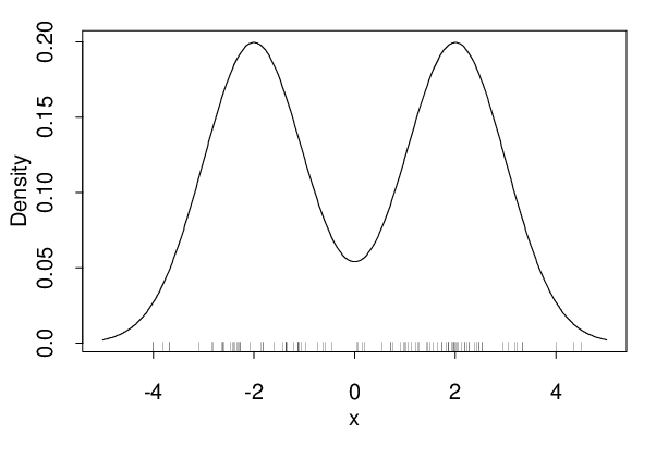
In order to demonstrate the power of the proposed methods, we present two simulation studies and illustrate the process of building mixture models.
Refer to captionRefer to caption

Refer to captionRefer to caption

Figure 4: (a) Simulated data from the two-component normal mixture: 0.5​N​(−2,1)+0.5​N​(2,1)0.5N(-2,1)+0.5N(2,1); (b) S⋆​(θ)S^{\star}(\theta) for the one-component mixture model; (c) S⋆​(θ)S^{\star}(\theta) for the two-component mixture model; (d) S⋆​(θ)S^{\star}(\theta) for the model with a third component included and the first component removed.

We consider the simulated dataset shown in Fig. 4(a), consisting of a sample of size n=100n=100 drawn from the two-component normal mixture model 0.5​N​(−2,1)+0.5​N​(2,1)0.5N(-2,1)+0.5N(2,1). The model building process starts with the first component at the sample mean θ^1=X¯=0.20322\widehat{\theta}_{1}=\overline{X}=0.20322. The starting model is obviously a poor fit for the dataset. Fig. 4(b) presents the fitted normalized score process S⋆​(θ)S^{\star}(\theta), showing two peaks in the vicinity of the true mixture components. An application of the volume-of-tube formula in (3.10) to this model yields κ0=5.72\kappa_{0}=5.72 and ℓ0=4\ell_{0}=4 with the critical value of c=2.518c=2.518 at the 5% level. Clearly the peaks are highly significant. A second component at θ2=−1.68929\theta_{2}=-1.68929 [the location of the larger left peak in Fig. 4(b)] is included in the model and the vector of estimated mixing weights is 𝜷^=(0.67315,0.32685)T\widehat{\boldsymbol{\beta}}=(0.67315,0.32685)^{T}. The incorrect first component θ1\theta_{1} still dominates the fitted mixture model.

The normalized score process relative to the two-component mixture is shown in Fig. 4(c). The striking feature of this plot is the two discontinuities at the fitted components θ1=0.203\theta_{1}=0.203 and θ2=−1.689\theta_{2}=-1.689. These discontinuities occur due to the zeroes of the covariance function since ℂ†​(θ1,θ1)=ℂ†​(θ2,θ2)=0\mathbb{C}^{{\dagger}}(\theta_{1},\theta_{1})=\mathbb{C}^{{\dagger}}(\theta_{2},\theta_{2})=0 which in turn corresponds to the singularities in S⋆​(θ)S^{\star}(\theta). The manifold ℳ\mathcal{M} for this process has three pieces so that κ0=5.082\kappa_{0}=5.082 and ℓ0=6\ell_{0}=6. The critical value c=2.571c=2.571 and the right peak is still highly significant. The maximum occurs at θ^3=2.07328\widehat{\theta}_{3}=2.07328 which is included as a third component in the model. Since 𝜷^=(0,0.45616,0.54384)T\widehat{\boldsymbol{\beta}}=(0,0.45616,0.54384)^{T}, the first component is removed from the model. For the two-component mixture model with θ^2\widehat{\theta}_{2} and θ^3\widehat{\theta}_{3}, the constants κ0=5.082\kappa_{0}=5.082 and ℓ0=6\ell_{0}=6 yielding c=2.571c=2.571. Fig. 4(d) presents the process S⋆​(θ)S^{\star}(\theta) and it is entirely below the critical value cc; therefore, the two-component mixture model with θ^2\widehat{\theta}_{2} and θ^3\widehat{\theta}_{3} is the final fitted model.

The true density is chosen as p⁡(x,η,θ)=0.5​(1−η)​ψ​(x,−2)+η​ψ​(x,0)+0.5​(1−η)​ψ​(x,2)p(x;\eta,\theta)=0.5(1-\eta)\,\psi(x;-2)+\eta\,\psi(x;0)+0.5(1-\eta)\,\psi(x;2) for η∈{0,0.1,0.2}\eta\in\{0,0.1,0.2\} and ψ⁡(⋅,θ)\psi(\cdot;\theta) is the normal density with mean θ\theta and unit variance. This density has two large with well separated components and our goal is to test for the presence of the poorly separated third component. We present simulation studies using 1000 data sets under the following three different scenarios:
Model 1: f⁡(x,𝝀)≡g⁡(x,𝒬)=[0.5​ψ​(x,−2)+0.5​ψ​(x,2)]f(x;\boldsymbol{\lambda})\equiv{\rm g}(x;\mathcal{Q})=[0.5\,\psi(x;-2)+0.5\,\psi(x;2)] is completely specified.
Model 2: f⁡(x,𝝀)≡g⁡(x,𝒬)=[β1​ψ​(x,−2)+β2​ψ​(x,2)]f(x;\boldsymbol{\lambda})\equiv{\rm g}(x;\mathcal{Q})=[\beta_{1}\,\psi(x;-2)+\beta_{2}\,\psi(x;2)], where β1\beta_{1} and β2\beta_{2} are estimated.
Model 3: f⁡(x,𝝀)≡g⁡(x,𝒬)=[β1​ψ​(x,θ1)+β2​ψ​(x,θ2)]f(x;\boldsymbol{\lambda})\equiv{\rm g}(x;\mathcal{Q})=[\beta_{1}\,\psi(x;\theta_{1})+\beta_{2}\,\psi(x;\theta_{2})], where β\betas and θ\thetas are estimated.

Table 1: Rejection rates for three different null models under three different perturbation sizes based on 1000 simulation studies.

n=200n=200 n=1000n=1000 Model η=0.0\eta=0.0 η=0.1\eta=0.1 η=0.2\eta=0.2 η=0.0\eta=0.0 η=0.05\eta=0.05 η=0.1\eta=0.1 1 79 537 975 74 636 990 2 78 583 985 76 673 992 3 74 292 588 61 371 817

Table 1 presents the rejection rates for 1000 simulations under two sample sizes. When η=0\eta=0, ℋ0\mathcal{H}_{0} is true and hence we expect the rejection rate to be close to the nominal significance level of 5%5\%. As η\eta increases, the power increases as expected. As the null assumptions are relaxed, the power decreases which again is to be expected. The poor separation between the components makes it difficult for the test to detect the third component which is more prominent for model 3. Naturally, estimating the nuisance parameters under the null model has an effect on the power of the test.

6 Discussion

In this article, we introduced a general class of models, perturbation models, and proposed a test statistic (asymptotically equivalent to the LRT statistic) based on the score process to detect the presence of perturbation. We derived general inferential theory for the asymptotic null distribution of the test statistic for a class of non-regular problems using the Hotelling-Weyl-Naiman volume-of-tube formula. The resulting theory is extended to solve the long-pending fundamental problem of testing for the mixture complexity, including the case when the null model includes a set of nuisance parameters. Our theory is applicable to a general family of mixture models including the multivariate family of mixtures. Other applications to the general theory include spatial scan analysis, latent class models (employed in social research) and Rasch models (employed in educational testing and survey sampling). The inferential theory developed in this article provides a solution to an important class of statistical problems involving loss of identifiability and/or when some of the parameters are on the boundary of the parametric space.

The explicit determination of the geometric constants appearing in the tube formula are carried out using the Libtube software (Loader, 2005). Our theory is general enough to be applicable to scalar or vector 𝝀\boldsymbol{\lambda} and univariate or multivariate data. The advantage of our approach is that the tube formula provides an elegant approximation to the asymptotic null distribution compared to those based on simulations or bootstrap based procedures.

7 Proofs

In this section we provide proofs of the main theorems. As before, notation ′\prime is used to denote derivative with respect to the appropriate term.

Proof of Theorem 2. Let

K⁡(η,𝜽)=∑i=1nlog⁡[1+η⁡{ψ⁡(xi,𝜽)−f⁡(xi,𝝀)}f⁡(xi,𝝀)].\displaystyle K(\eta,\boldsymbol{\theta})=\sum_{i=1}^{n}\log\left[1+\frac{\eta\,\left\{\psi(x_{i};\boldsymbol{\theta})-f(x_{i};\boldsymbol{\lambda})\right\}}{f(x_{i};\boldsymbol{\lambda})}\right].

The LRT statistic becomes sup𝜽,η>0K⁡(η,𝜽)\sup_{\boldsymbol{\theta},\eta>0}K(\eta,\boldsymbol{\theta}). For any η>0\eta>0, a Taylor series expansion yields

K⁡(η/n,𝜽)\displaystyle K(\eta/\sqrt{n},\boldsymbol{\theta}) =\displaystyle= K⁡(0,𝜽)+ηn​K′​(0,𝜽)+η22​n​K′′​(η⋆,𝜽)for0≤η⋆≤ηn\displaystyle K(0,\boldsymbol{\theta})+\frac{\eta}{\sqrt{n}}K^{\prime}(0,\boldsymbol{\theta})+\frac{\eta^{2}}{2n}K^{\prime\prime}(\eta^{\star},\boldsymbol{\theta})\quad\mbox{for}\quad 0\leq\eta^{\star}\leq\frac{\eta}{\sqrt{n}}
=\displaystyle= ηn​∑i=1n[ψ⁡(xi,𝜽)f⁡(xi,𝝀)−1]\displaystyle\frac{\eta}{\sqrt{n}}\sum_{i=1}^{n}\left[\frac{\psi(x_{i};\boldsymbol{\theta})}{f(x_{i};\boldsymbol{\lambda})}-1\right]
−η22​n∑i=1n[{ψ⁡(xi,𝜽)−f⁡(xi,𝝀)}2/{f⁡(xi,𝝀)}21+η⋆​{ψ⁡(xi,𝜽)/f⁡(xi,𝝀)−1}].\displaystyle-\,\frac{\eta^{2}}{2n}\sum_{i=1}^{n}\left[\frac{\left\{\psi(x_{i};\boldsymbol{\theta})-f(x_{i};\boldsymbol{\lambda})\right\}^{2}/\{f(x_{i};\boldsymbol{\lambda})\}^{2}}{1+\eta^{\star}\{\psi(x_{i};\boldsymbol{\theta})/f(x_{i};\boldsymbol{\lambda})-1\}}\right].

Under an implicit assumption that convergence statements are uniform in 𝜽\boldsymbol{\theta} for bounded sets and from the results in Rubin, 1956, it follows that

K′′​(η⋆,𝜽)=∑i=1n[{ψ⁡(xi,𝜽)−f⁡(xi,𝝀)}2/{f⁡(xi,𝝀)}21+η⋆​{ψ⁡(xi,𝜽)/f⁡(xi,𝝀)−1}]\displaystyle K^{\prime\prime}(\eta^{\star},\boldsymbol{\theta})=\sum_{i=1}^{n}\left[\frac{\left\{\psi(x_{i};\boldsymbol{\theta})-f(x_{i};\boldsymbol{\lambda})\right\}^{2}/\{f(x_{i};\boldsymbol{\lambda})\}^{2}}{1+\eta^{\star}\{\psi(x_{i};\boldsymbol{\theta})/f(x_{i};\boldsymbol{\lambda})-1\}}\right]

is uniformly converging to ℂ⁡(𝜽,𝜽)\mathbb{C}(\boldsymbol{\theta},\boldsymbol{\theta}). Therefore,

K⁡(η/n,𝜽)\displaystyle K(\eta/\sqrt{n},\boldsymbol{\theta}) =\displaystyle= ηn​S​(𝜽)−η22​ℂ​(𝜽,𝜽)+op​(1),\displaystyle\frac{\eta}{\sqrt{n}}S(\boldsymbol{\theta})-\frac{\eta^{2}}{2}\mathbb{C}(\boldsymbol{\theta},\boldsymbol{\theta})+o_{p}(1),

where the op​(1)o_{p}(1) term is uniform in η\eta and 𝜽\boldsymbol{\theta} on compact sets. In effect, supη≥0K⁡(η/n,𝜽)=(1/2)​max⁡{0,S⋆​(𝜽)}2+op​(1)\sup_{\eta\geq 0}K(\eta/\sqrt{n},\boldsymbol{\theta})=(1/2)\max\{0,S^{\star}(\boldsymbol{\theta})\}^{2}+o_{p}(1).  

On the way to proving Theorem 3, we derive a series of technical results.

Lemma 2

Let a⁡(θ)a(\theta) be a continuously differentiable function on an interval Θ\Theta. Let a⋆=[a⁡(θ1)−a⁡(θ0)]a_{\star}=[a(\theta_{1})-a(\theta_{0})]. Then

∫θ0θ1[a′​(θ)]2​𝑑θ≥a⋆2|θ1−θ0|,\displaystyle\int_{\theta_{0}}^{\theta_{1}}[a^{\prime}(\theta)]^{2}\,d\theta\geq\frac{a_{\star}^{2}}{|\theta_{1}-\theta_{0}|},

where a′​(θ)=d​a​(θ)/d​θa^{\prime}(\theta)=da(\theta)/d\theta.

Proof. Let θ⋆=(θ1−θ0)\theta_{\star}=(\theta_{1}-\theta_{0}) so that

∫θ0θ1[a′​(θ)]2​𝑑θ\displaystyle\int_{\theta_{0}}^{\theta_{1}}[a^{\prime}(\theta)]^{2}\,d\theta =\displaystyle= ∫θ0θ1(a′​(θ)−a⋆θ⋆+a⋆θ⋆)2​𝑑θ\displaystyle\int_{\theta_{0}}^{\theta_{1}}\left(a^{\prime}(\theta)-\frac{a_{\star}}{\theta_{\star}}+\frac{a_{\star}}{\theta_{\star}}\right)^{2}\,d\theta
=\displaystyle= ∫θ0θ1(a′​(θ)−a⋆θ⋆)2​𝑑θ+∫θ0θ1a⋆2θ⋆2​𝑑θ+2​a⋆θ⋆​∫θ0θ1(a′​(θ)−a⋆θ⋆)​𝑑θ.\displaystyle\int_{\theta_{0}}^{\theta_{1}}\left(a^{\prime}(\theta)-\frac{a_{\star}}{\theta_{\star}}\right)^{2}\,d\theta+\int_{\theta_{0}}^{\theta_{1}}\frac{a_{\star}^{2}}{\theta_{\star}^{2}}\,d\theta+\frac{2a_{\star}}{\theta_{\star}}\int_{\theta_{0}}^{\theta_{1}}\left(a^{\prime}(\theta)-\frac{a_{\star}}{\theta_{\star}}\right)\,d\theta.

Note that the first integral is non-negative and the third one is zero.  

Lemma 3

Suppose θ0<θ2\theta_{0}<\theta_{2} and a⁡(θ0)=a⁡(θ2)=0a(\theta_{0})=a(\theta_{2})=0, then

∫Θ[a′​(θ)]2​𝑑θ≥4|θ2−θ0|​(supθ0≤θ≤θ2|a⁡(θ)|)2.\displaystyle\int_{\Theta}[a^{\prime}(\theta)]^{2}\,d\theta\geq\frac{4}{|\theta_{2}-\theta_{0}|}\left(\sup_{\theta_{0}\leq\theta\leq\theta_{2}}|a(\theta)|\right)^{2}.

Proof. Suppose the supremum occurs at (θ1,a⋆)(\theta_{1},a_{\star}) with θ0<θ1<θ2\theta_{0}<\theta_{1}<\theta_{2}. An application of Lemma 2 separately over [θ0,θ1][\theta_{0},\theta_{1}] and [θ1,θ2][\theta_{1},\theta_{2}] yields

∫Θ[a′​(θ)]2​𝑑θ≥∫θ0θ2[a′​(θ)]2​𝑑θ≥a⋆2​[1(θ1−θ0)+1(θ2−θ1)]≥4​a⋆2(θ2−θ0).\displaystyle\int_{\Theta}[a^{\prime}(\theta)]^{2}\,d\theta\geq\int_{\theta_{0}}^{\theta_{2}}[a^{\prime}(\theta)]^{2}\,d\theta\geq a_{\star}^{2}\left[\frac{1}{(\theta_{1}-\theta_{0})}+\frac{1}{(\theta_{2}-\theta_{1})}\right]\geq\frac{4a_{\star}^{2}}{(\theta_{2}-\theta_{0})}.
 
Lemma 4

Suppose b⁡(θ)b(\theta) is continuously differentiable. For δ>0\delta>0, let bδ​(θ)b_{\delta}(\theta) be the linear interpolant between the points 0,±δ,±2​δ,…0,\pm\delta,\pm 2\delta,\ldots. Then

sup𝜽∈𝚯|bδ​(θ)−b⁡(θ)|2≤δ​∫Θ[b′​(θ)]2​𝑑θ.\displaystyle\sup_{\boldsymbol{\theta}\,\in\,\boldsymbol{\Theta}}\Big|b_{\delta}(\theta)-b(\theta)\Big|^{2}\leq\delta\int_{\Theta}[b^{\prime}(\theta)]^{2}\,d\theta.

Proof. Once again, let a⋆a_{\star} be the supremum. An application of Lemma 3 to a⁡(θ)=[bδ​(θ)−b⁡(θ)]a(\theta)=[b_{\delta}(\theta)-b(\theta)] yields

a⋆2\displaystyle a_{\star}^{2} ≤\displaystyle\leq δ4​∫Θ[bδ′​(θ)−b′​(θ)]2​𝑑θ≤δ2​∫Θ[{bδ′​(θ)}2+{b′​(θ)}2]​𝑑θ\displaystyle\frac{\delta}{4}\int_{\Theta}\left[b^{\prime}_{\delta}(\theta)-b^{\prime}(\theta)\right]^{2}\,d\theta\leq\frac{\delta}{2}\int_{\Theta}\left[\{b^{\prime}_{\delta}(\theta)\}^{2}+\{b^{\prime}(\theta)\}^{2}\right]\,d\theta
≤\displaystyle\leq δ​∫Θ[b′​(θ)]2​𝑑θ.\displaystyle\delta\int_{\Theta}[b^{\prime}(\theta)]^{2}\,d\theta.

The final inequality holds since ∫Θ[bδ′​(θ)]2​𝑑θ≤∫Θ[b′​(θ)]2\int_{\Theta}[b^{\prime}_{\delta}(\theta)]^{2}\,d\theta\leq\int_{\Theta}[b^{\prime}(\theta)]^{2}; this follows from the application of Lemma 2 between each pair of knots of bδ​(⋅)b_{\delta}(\cdot).  

Lemma 5

Let Y⁡(𝛉)Y(\boldsymbol{\theta}) be a stochastic process with continuously differentiable sample paths and let Yδ​(𝛉)Y_{\delta}(\boldsymbol{\theta}) be its linear interpolant between points 0,±δ,…0,\pm\delta,\ldots. Then

ℙ⁡(sup𝜽∈𝚯|Yδ​(𝜽)−Y⁡(𝜽)|≥ϵ)≤δϵ2​𝔼​∫𝚯[Y′​(𝜽)]2​𝑑𝜽.\mathbb{P}\left(\sup_{\boldsymbol{\theta}\,\in\,\boldsymbol{\Theta}}|Y_{\delta}(\boldsymbol{\theta})-Y(\boldsymbol{\theta})|\geq\epsilon\right)\leq\frac{\delta}{\epsilon^{2}}\,\mathbb{E}\int_{\boldsymbol{\Theta}}[Y^{\prime}(\boldsymbol{\theta})]^{2}\,d\boldsymbol{\theta}.

Uniform convergence holds if the expectation is finite:

limδ→0ℙ⁡(sup𝜽∈𝚯|Yδ​(𝜽)−Y⁡(𝜽)|≥ϵ)=0for allϵ>0.\lim_{\delta\to 0}\mathbb{P}\left(\sup_{\boldsymbol{\theta}\,\in\,\boldsymbol{\Theta}}|Y_{\delta}(\boldsymbol{\theta})-Y(\boldsymbol{\theta})|\geq\epsilon\right)=0\quad\mbox{for all}\quad\epsilon>0. (7.1)

Proof. From Lemma 4, it follows that

ℙ⁡(sup𝜽∈𝚯|Yδ​(𝜽)−Y⁡(𝜽)|≥ϵ)\displaystyle\mathbb{P}\left(\sup_{\boldsymbol{\theta}\,\in\,\boldsymbol{\Theta}}|Y_{\delta}(\boldsymbol{\theta})-Y(\boldsymbol{\theta})|\geq\epsilon\right) ≤\displaystyle\leq ℙ⁡(δ​∫𝚯[Y′​(𝜽)]2​𝑑𝜽≥ϵ2)\displaystyle\mathbb{P}\left(\delta\int_{\boldsymbol{\Theta}}[Y^{\prime}(\boldsymbol{\theta})]^{2}\,d\boldsymbol{\theta}\geq\epsilon^{2}\right)
≤\displaystyle\leq δϵ2​𝔼​∫𝚯[Y′​(𝜽)]2​𝑑𝜽,\displaystyle\frac{\delta}{\epsilon^{2}}\,\mathbb{E}\int_{\boldsymbol{\Theta}}[Y^{\prime}(\boldsymbol{\theta})]^{2}\,d\boldsymbol{\theta},

where the last line follows from the Markov’s inequality for any non-negative random variable.  

Lemma 6

If Yδ​(𝛉)Y_{\delta}(\boldsymbol{\theta}) converges uniformly to Y⁡(𝛉)Y(\boldsymbol{\theta}), as defined in (7.1), then

limδ→0ℙ⁡(sup𝜽∈𝚯Yδ​(𝜽)≥c)=ℙ⁡(sup𝜽∈𝚯Y⁡(𝜽)≥c)for anyc,\displaystyle\lim_{\delta\to 0}\mathbb{P}\left(\sup_{\boldsymbol{\theta}\,\in\,\boldsymbol{\Theta}}Y_{\delta}(\boldsymbol{\theta})\geq c\right)=\mathbb{P}\left(\sup_{\boldsymbol{\theta}\,\in\,\boldsymbol{\Theta}}Y(\boldsymbol{\theta})\geq c\right)\quad\mbox{for any}\quad c,

where the right hand side is continuous.

Proof. For any ϵ>0\epsilon>0,

ℙ⁡(sup𝜽∈𝚯Yδ​(𝜽)≥c)≥ℙ⁡(sup𝜽∈𝚯Y⁡(𝜽)≥c+ϵ)−ℙ⁡(sup𝜽∈𝚯|Yδ​(𝜽)−Y⁡(𝜽)|>ϵ).\displaystyle\mathbb{P}\left(\sup_{\boldsymbol{\theta}\,\in\,\boldsymbol{\Theta}}Y_{\delta}(\boldsymbol{\theta})\geq c\right)\geq\mathbb{P}\left(\sup_{\boldsymbol{\theta}\,\in\,\boldsymbol{\Theta}}Y(\boldsymbol{\theta})\geq c+\epsilon\right)-\mathbb{P}\left(\sup_{\boldsymbol{\theta}\,\in\,\boldsymbol{\Theta}}|Y_{\delta}(\boldsymbol{\theta})-Y(\boldsymbol{\theta})|>\epsilon\right).

Consequently, lim infδ→0ℙ⁡(sup𝜽∈𝚯Yδ​(𝜽)≥c)≥ℙ⁡(sup𝜽∈𝚯Y⁡(𝜽)≥c+ϵ)\liminf_{\delta\to 0}\,\mathbb{P}\left(\sup_{\boldsymbol{\theta}\,\in\,\boldsymbol{\Theta}}Y_{\delta}(\boldsymbol{\theta})\geq c\right)\geq\mathbb{P}\left(\sup_{\boldsymbol{\theta}\,\in\,\boldsymbol{\Theta}}Y(\boldsymbol{\theta})\geq c+\epsilon\right). However, since ϵ\epsilon is arbitrary,

lim infδ→0ℙ⁡(sup𝜽∈𝚯Yδ​(𝜽)≥c)≥ℙ⁡(sup𝜽∈𝚯Y⁡(𝜽)≥c).\displaystyle\liminf_{\delta\to 0}\,\mathbb{P}\left(\sup_{\boldsymbol{\theta}\,\in\,\boldsymbol{\Theta}}Y_{\delta}(\boldsymbol{\theta})\geq c\right)\geq\mathbb{P}\left(\sup_{\boldsymbol{\theta}\,\in\,\boldsymbol{\Theta}}Y(\boldsymbol{\theta})\geq c\right).

By a similar argument, it follows that

lim supδ→0ℙ⁡(sup𝜽∈𝚯Yδ​(𝜽))≥ℙ⁡(sup𝜽∈𝚯Y⁡(𝜽)≥c)\displaystyle\limsup_{\delta\to 0}\,\mathbb{P}\left(\sup_{\boldsymbol{\theta}\,\in\,\boldsymbol{\Theta}}Y_{\delta}(\boldsymbol{\theta})\right)\geq\mathbb{P}\left(\sup_{\boldsymbol{\theta}\,\in\,\boldsymbol{\Theta}}Y(\boldsymbol{\theta})\geq c\right)

which completes the proof.  

Proof of Theorem 3. First, convergence of finite-dimensional distributions is a consequence of the multivariate central limit theorem. Since a linear interpolant is always maximized at one of the knots, this implies that the theorem holds for a linear interpolant:

limn→∞ℙ⁡(sup𝜽∈𝚯Sδ⋆​(𝜽)≥c)=ℙ⁡(sup𝜽∈𝚯Zδ​(𝜽)≥c)\lim_{n\to\infty}\mathbb{P}\left(\sup_{\boldsymbol{\theta}\,\in\,\boldsymbol{\Theta}}S_{\delta}^{\star}(\boldsymbol{\theta})\geq c\right)=\mathbb{P}\left(\sup_{\boldsymbol{\theta}\,\in\,\boldsymbol{\Theta}}Z_{\delta}(\boldsymbol{\theta})\geq c\right)

for any δ>0\delta>0. For any ϵ>0\epsilon>0, Lemma 5 implies that

ℙ⁡(sup𝜽∈𝚯S⋆​(𝜽)≥c)\displaystyle\mathbb{P}\left(\sup_{\boldsymbol{\theta}\,\in\,\boldsymbol{\Theta}}S^{\star}(\boldsymbol{\theta})\geq c\right) ≤\displaystyle\leq ℙ⁡(sup𝜽∈𝚯Sδ⋆​(𝜽)≥c−ϵ)+ℙ⁡(sup𝜽∈𝚯|S⋆​(𝜽)−Sδ⋆​(𝜽)|≥ϵ)\displaystyle\mathbb{P}\left(\sup_{\boldsymbol{\theta}\,\in\,\boldsymbol{\Theta}}S_{\delta}^{\star}(\boldsymbol{\theta})\geq c-\epsilon\right)+\mathbb{P}\left(\sup_{\boldsymbol{\theta}\,\in\,\boldsymbol{\Theta}}|S^{\star}(\boldsymbol{\theta})-S_{\delta}^{\star}(\boldsymbol{\theta})|\geq\epsilon\right)
≤\displaystyle\leq ℙ⁡(sup𝜽∈𝚯Sδ⋆​(𝜽)≥c−ϵ)+δϵ2​𝔼​∫𝚯(∂∂𝜽​Sδ⋆​(𝜽))2​𝑑𝜽\displaystyle\mathbb{P}\left(\sup_{\boldsymbol{\theta}\,\in\,\boldsymbol{\Theta}}S_{\delta}^{\star}(\boldsymbol{\theta})\geq c-\epsilon\right)+\frac{\delta}{\epsilon^{2}}\,\mathbb{E}\int_{\boldsymbol{\Theta}}\left({\frac{\partial}{\partial\boldsymbol{\theta}}S_{\delta}^{\star}(\boldsymbol{\theta})}\right)^{2}\,d\boldsymbol{\theta}
=\displaystyle= ℙ⁡(sup𝜽∈𝚯Sδ⋆​(𝜽)≥c−ϵ)+δϵ2​𝔼​∫𝚯[Zδ′​(𝜽)]2​𝑑𝜽,\displaystyle\mathbb{P}\left(\sup_{\boldsymbol{\theta}\,\in\,\boldsymbol{\Theta}}S_{\delta}^{\star}(\boldsymbol{\theta})\geq c-\epsilon\right)+\frac{\delta}{\epsilon^{2}}\,\mathbb{E}\int_{\boldsymbol{\Theta}}\left[Z_{\delta}^{\prime}(\boldsymbol{\theta})\right]^{2}\,d\boldsymbol{\theta},

where Zδ′​(𝜽)=∂Zδ​(𝜽)/∂𝜽Z_{\delta}^{\prime}(\boldsymbol{\theta})=\partial Z_{\delta}(\boldsymbol{\theta})/\partial\boldsymbol{\theta}. The last equality follows from the fact that ZδZ_{\delta} and Sδ⋆S_{\delta}^{\star} have the same covariance function. Assumption 3 implies that the expectation is finite. From the convergence of finite-dimensional distributions, it follows that

lim supn→∞ℙ⁡(sup𝜽∈𝚯S⋆​(𝜽)≥c)≤ℙ⁡(sup𝜽∈𝚯Zδ​(𝜽)≥c−ϵ)+δϵ2​𝔼​∫𝚯[Zδ′​(𝜽)]2​𝑑𝜽.\displaystyle\limsup_{n\to\infty}\,\mathbb{P}\left(\sup_{\boldsymbol{\theta}\,\in\,\boldsymbol{\Theta}}S^{\star}(\boldsymbol{\theta})\geq c\right)\leq\mathbb{P}\left(\sup_{\boldsymbol{\theta}\,\in\,\boldsymbol{\Theta}}Z_{\delta}(\boldsymbol{\theta})\geq c-\epsilon\right)+\frac{\delta}{\epsilon^{2}}\,\mathbb{E}\int_{\boldsymbol{\Theta}}\left[Z_{\delta}^{\prime}(\boldsymbol{\theta})\right]^{2}\,d\boldsymbol{\theta}.

First, let δ→0\delta\to 0 and apply Lemma 6 to ZδZ_{\delta}. Next, let ϵ→0\epsilon\to 0 to obtain

lim supn→∞ℙ⁡(sup𝜽∈𝚯S⋆​(𝜽)≥c)≤ℙ⁡(sup𝜽∈𝚯Z⁡(𝜽)≥c).\displaystyle\limsup_{n\to\infty}\,\mathbb{P}\left(\sup_{\boldsymbol{\theta}\,\in\,\boldsymbol{\Theta}}S^{\star}(\boldsymbol{\theta})\geq c\right)\leq\mathbb{P}\left(\sup_{\boldsymbol{\theta}\,\in\,\boldsymbol{\Theta}}Z(\boldsymbol{\theta})\geq c\right).

A similar argument shows that

lim infn→∞ℙ⁡(sup𝜽∈𝚯S⋆​(𝜽)≥c)≥ℙ⁡(sup𝜽∈𝚯Z⁡(𝜽)≥c)\displaystyle\liminf_{n\to\infty}\,\mathbb{P}\left(\sup_{\boldsymbol{\theta}\,\in\,\boldsymbol{\Theta}}S^{\star}(\boldsymbol{\theta})\geq c\right)\geq\mathbb{P}\left(\sup_{\boldsymbol{\theta}\,\in\,\boldsymbol{\Theta}}Z(\boldsymbol{\theta})\geq c\right)

which completes the proof.  

Proof of Theorem 4. We assume the regularity conditions 1 to 4 in Adler, 2000. The integral in (3.8) can be expressed as

∫c2∞ℙ⁡(sup𝜽∈𝚯⟨𝐔J,𝝃J​(𝜽)⟩≥cy)​hJ​(y)​𝑑y\displaystyle\int_{c^{2}}^{\infty}\mathbb{P}\left(\sup_{\boldsymbol{\theta}\,\in\,\boldsymbol{\Theta}}\,\left<{\mathbf{U}_{J}},{\boldsymbol{\xi}_{J}(\boldsymbol{\theta})}\right>\geq\frac{c}{\sqrt{y}}\right)h_{J}(y)\,dy =\displaystyle= ∫c2c2w0ℙ⁡(sup𝜽∈𝚯⟨𝐔J,𝝃J​(𝜽)⟩≥cy)​hJ​(y)​𝑑y\displaystyle\int_{c^{2}}^{\frac{c^{2}}{w_{0}}}\mathbb{P}\left(\sup_{\boldsymbol{\theta}\,\in\,\boldsymbol{\Theta}}\,\left<{\mathbf{U}_{J}},{\boldsymbol{\xi}_{J}(\boldsymbol{\theta})}\right>\geq\frac{c}{\sqrt{y}}\right)h_{J}(y)\,dy
+∫c2w0∞ℙ(sup𝜽∈𝚯⟨𝐔J,𝝃J(𝜽)⟩≥cy)hJ(y)dy,\displaystyle+\int_{\frac{c^{2}}{w_{0}}}^{\infty}\mathbb{P}\left(\sup_{\boldsymbol{\theta}\,\in\,\boldsymbol{\Theta}}\,\left<{\mathbf{U}_{J}},{\boldsymbol{\xi}_{J}(\boldsymbol{\theta})}\right>\geq\frac{c}{\sqrt{y}}\right)h_{J}(y)\,dy,

where w0=(1−r02/2)w_{0}=(1-r_{0}^{2}/2) and r0r_{0} is the critical radius of the tube. The volume-of-tube formula given in (A.4) is exact when y∈[c2,c2/w0]y\in[c^{2},c^{2}/w_{0}] and it is only approximate when y∈[c2/w0,∞)y\in[c^{2}/w_{0},\infty). In the former case, from (3.9)

ℙ(sup𝜽∈𝚯⟨𝐔J,𝝃J(𝜽)⟩≥cy)=∑t=0dζtJAd+1−tℙ[B(d+1−t)/2,(J−d−1+t)/2≥w2].\displaystyle\mathbb{P}\left(\sup_{\boldsymbol{\theta}\,\in\,\boldsymbol{\Theta}}\,\left<{\mathbf{U}_{J}},{\boldsymbol{\xi}_{J}(\boldsymbol{\theta})}\right>\geq\frac{c}{\sqrt{y}}\right)=\sum_{t=0}^{d}\frac{\zeta_{t}^{J}}{A_{d+1-t}}\mathbb{P}\left[B_{(d+1-t)/2,(J-d-1+t)/2}\geq w^{2}\right].

We express the first integral in () as F⁡(c2)−F⁡(c2/w0)F(c^{2})-F(c^{2}/w_{0}), where

F(x)=∑t=0dζtJAd+1−t∫x∞ℙ[B(d+1−t)/2,(J−d−1+t)/2≥w2]hJ(y)dy.\displaystyle F(x)=\sum_{t=0}^{d}\frac{\zeta_{t}^{J}}{A_{d+1-t}}\int_{x}^{\infty}\mathbb{P}\left[B_{(d+1-t)/2,(J-d-1+t)/2}\geq w^{2}\right]h_{J}(y)\,dy.

Note that the second integral in () is ≥0\geq 0 providing a lower bound. Furthermore,

∫c2/w0∞ℙ⁡(sup𝜽∈𝚯⟨𝐔J,𝝃J​(𝜽)⟩≥cy)​hJ​(y)​𝑑y≤∫c2/w0∞hJ​(y)​𝑑y=ℙ⁡(χJ2≥c2w0).\displaystyle\int_{c^{2}/w_{0}}^{\infty}\mathbb{P}\left(\sup_{\boldsymbol{\theta}\,\in\,\boldsymbol{\Theta}}\,\left<{\mathbf{U}_{J}},{\boldsymbol{\xi}_{J}(\boldsymbol{\theta})}\right>\geq\frac{c}{\sqrt{y}}\right)h_{J}(y)\,dy\leq\int_{c^{2}/w_{0}}^{\infty}h_{J}(y)dy=\mathbb{P}\left(\chi^{2}_{J}\geq\frac{c^{2}}{w_{0}}\right).

Therefore, F(c2)−F(c2/w0)≤ℙ[sup𝜽∈𝚯ZJ(𝜽)≥c]≤F(c2)−F(c2/w0)+ℙ(χJ2≥c2/w0)F(c^{2})-F(c^{2}/w_{0})\leq\mathbb{P}\left[\sup_{\boldsymbol{\theta}\,\in\,\boldsymbol{\Theta}}\,Z_{J}(\boldsymbol{\theta})\geq c\right]\leq F(c^{2})-F(c^{2}/w_{0})+\mathbb{P}\left(\chi^{2}_{J}\geq c^{2}/w_{0}\right). As c→∞c\to\infty, F⁡(c2)−F⁡(c2/w0)≈F⁡(c2)F(c^{2})-F(c^{2}/w_{0})\approx F(c^{2}). Therefore, ℙ⁡(sup𝜽∈𝚯ZJ​(𝜽)≥c)≈F⁡(c2)\mathbb{P}\left(\sup_{\boldsymbol{\theta}\,\in\,\boldsymbol{\Theta}}\,Z_{J}(\boldsymbol{\theta})\geq c\right)\approx F(c^{2}) as c→∞c\to\infty. By performing the integration in F⁡(c2)F(c^{2}), it follows that

ℙ(sup𝜽∈𝚯ZJ(𝜽)≥c)=∑t=0dζtJAd+1−tℙ(χd+1−t2≥c2)+o[c−1exp(−c2/2)]asc→∞.\displaystyle\mathbb{P}\left(\sup_{\boldsymbol{\theta}\,\in\,\boldsymbol{\Theta}}\,Z_{J}(\boldsymbol{\theta})\geq c\right)=\sum_{t=0}^{d}\frac{\zeta_{t}^{J}}{A_{d+1-t}}\mathbb{P}\left(\chi^{2}_{d+1-t}\geq c^{2}\right)+o[c^{-1}\exp(-c^{2}/2)]\quad\mbox{as}\quad c\to\infty.

When the Karhunen-Loève expansion is infinite, the above result for the truncated Gaussian random field ZJ​(𝜽)Z_{J}(\boldsymbol{\theta}) is extended by letting J→∞J\to\infty as follows. Uniform convergence of the Karhunen-Loève expansion implies that ZJ​(𝜽)⟶Z⁡(𝜽)Z_{J}(\boldsymbol{\theta})\longrightarrow Z(\boldsymbol{\theta}) uniformly and hence

ℙ⁡(sup𝜽∈𝚯ZJ​(𝜽)≥c)⟶ℙ⁡(sup𝜽∈𝚯Z⁡(𝜽)≥c)asJ→∞.\displaystyle\mathbb{P}\left(\sup_{\boldsymbol{\theta}\,\in\,\boldsymbol{\Theta}}Z_{J}(\boldsymbol{\theta})\geq c\right)\longrightarrow\mathbb{P}\left(\sup_{\boldsymbol{\theta}\,\in\,\boldsymbol{\Theta}}Z(\boldsymbol{\theta})\geq c\right)\quad\mbox{as}\quad J\to\infty. (7.3)

The volume-of-tube formula given in (A.4) is in terms of ζtJ\zeta^{J}_{t}; however, as J→∞J\to\infty and for t=0,…,dt=0,\ldots,d, ζtJ→ζt\zeta^{J}_{t}\to\zeta_{t}, the corresponding geometric term found via ρ⁡(𝜽,𝜽)\rho(\boldsymbol{\theta},\boldsymbol{\theta}), Therefore the result (3.10) holds. For example, the expression for κ0≡ζ0\kappa_{0}\equiv\zeta_{0} is derived by approximating ℳ\mathcal{M} by a series of short line segments to obtain

κ0=∫𝜽|det[∇1∇2T​ρ​(𝜽,𝜽)]|1/2​𝑑𝜽. \kappa_{0}=\int_{\boldsymbol{\theta}}\Big|\det\left[\nabla_{1}\nabla_{2}^{T}\rho(\boldsymbol{\theta},\boldsymbol{\theta})\right]\Big|^{1/2}d\boldsymbol{\theta}.\quad\quad\quad\quad\hfill\rule{5.69054pt}{5.69054pt}

Remark 3: We take sufficiently large JJ so that the relation (7.3) holds. In practice, it is not necessary to employ a truncated covariance function (3.7) that requires specification of JJ and the manifold ℳ\mathcal{M}. Our calculations are carried out in terms of the covariance function ℂ⁡(𝜽,𝜽†)\mathbb{C}(\boldsymbol{\theta},\boldsymbol{\theta}^{{\dagger}}). In effect, knowledge of JJ and the specification of ℳ\mathcal{M} does not arise in practice.

Appendix A: Explicit Expressions for Geometric Constants in (3.10)

We consider finite Karhunen-Loève expansion with JJ terms in deriving the geometric constants. As a first step, we partition the manifold ℳ\mathcal{M}, correspondingly the tube 𝔗⁡(r,ℳ)\mathfrak{T}(r,\mathcal{M}) and the parameter space 𝚯\boldsymbol{\Theta} into various boundary regions. First, each point in 𝔗⁡(r,ℳ)\mathfrak{T}(r,\mathcal{M}) is linked to a point in ℳ\mathcal{M} by a perpendicular projection. Correspondingly, each point in ℳ\mathcal{M} is linked to a set of points in 𝔗⁡(r,ℳ)\mathfrak{T}(r,\mathcal{M}). Second, partition ℳ\mathcal{M} into regions ℳ0,…,ℳd\mathcal{M}_{0},\ldots,\mathcal{M}_{d} based on the dimension of the linked sets, where ℳ0\mathcal{M}_{0} represents the main part of the manifold and ℳ1,…,ℳd\mathcal{M}_{1},\ldots,\mathcal{M}_{d} represent boundary regions. For example, when d=1d=1, ℳ1\mathcal{M}_{1} corresponds to the two end-points and ℳ0\mathcal{M}_{0} corresponds to the rest of the tube (see Fig. 1). If d=2d=2, manifold ℳ\mathcal{M} is a polygon so that ℳ2\mathcal{M}_{2} represents the corners, ℳ1\mathcal{M}_{1} the edges and ℳ0\mathcal{M}_{0} the interior. In effect, for a dd-dimensional manifold ℳ\mathcal{M}, we can partition both 𝔗⁡(r,ℳ)\mathfrak{T}(r,\mathcal{M}) and the space 𝚯\boldsymbol{\Theta} into (d+1)(d+1) regions to express ϑ⁡(r,ℳ)=V0+V1+⋯+Vd\vartheta(r,\mathcal{M})=V_{0}+V_{1}+\cdots+V_{d}. The main part of the tube can be represented as

[(1+∥𝝉∥2)−1/2(𝝃(𝜽)+𝐐(𝜽)𝝉):𝜽∈𝚯,∥𝝉∥≤τ0],\left[(1+\|\boldsymbol{\tau}\|^{2})^{-1/2}\,\left(\boldsymbol{\xi}(\boldsymbol{\theta})+\mathbf{Q}(\boldsymbol{\theta})\,\boldsymbol{\tau}\right)\!:\boldsymbol{\theta}\in\boldsymbol{\Theta},\|\boldsymbol{\tau}\|\leq\tau_{0}\right], (A.1)

where τ0=1−w2/w\tau_{0}=\sqrt{1-w^{2}}/w, 𝐐⁡(𝜽)\mathbf{Q}(\boldsymbol{\theta}) is an orthonormal basis matrix for the normal space at 𝝃⁡(𝜽)\boldsymbol{\xi}(\boldsymbol{\theta}). Provided that this transformation is one-to-one, the volume V0V_{0} can be expressed as V0=∫𝜽∫𝝉|det[𝐉⁡(𝜽,𝝉)]|​𝑑𝜽​𝑑𝝉V_{0}=\int_{\boldsymbol{\theta}}\int_{\boldsymbol{\tau}}\Big|\det[\mathbf{J}(\boldsymbol{\theta},\boldsymbol{\tau})]\Big|\,d\boldsymbol{\theta}\,d\boldsymbol{\tau}, where 𝐉⁡(𝜽,𝝉)\mathbf{J}(\boldsymbol{\theta},\boldsymbol{\tau}) is the Jacobian of the representation (A.1). The determinant of the Jacobian can be expressed as det[𝐉(𝜽,𝝉)]=P𝜽(𝝉)(1+∥𝝉∥2)−n/2\det[\mathbf{J}(\boldsymbol{\theta},\boldsymbol{\tau})]=P_{\boldsymbol{\theta}}(\boldsymbol{\tau})(1+\|\boldsymbol{\tau}\|^{2})^{-n/2}, where P𝜽​(𝝉)P_{\boldsymbol{\theta}}(\boldsymbol{\tau}) is a ddth degree polynomial in 𝝉\boldsymbol{\tau} with coefficients depending on 𝜽\boldsymbol{\theta}. This representation allows the integral defining V0V_{0} to be split into its 𝜽\boldsymbol{\theta} and 𝝉\boldsymbol{\tau} components, leading to a finite series expansion, for a truncated ZJ​(𝜽)Z_{J}(\boldsymbol{\theta}),

V0=∑t=0dκt2​AJAt+1​Ad+1−tℙ[B(d+1−t)/2,(J−d−1+t)/2≥w2],V_{0}=\sum_{t=0}^{d}\kappa_{t}\frac{2A_{J}}{A_{t+1}A_{d+1-t}}\mathbb{P}\left[B_{(d+1-t)/2,(J-d-1+t)/2}\geq w^{2}\right],

where, κt\kappa_{t} are the polynomial coefficients integrated over ℳ\mathcal{M} for even-order tt and the partial beta terms arise from integrating the τ\tau parts. Odd-order terms integrate to 0 by symmetry; therefore, we set κt=0\kappa_{t}=0 when tt is odd. Recall that At=2​πt/2/Γ⁡(t/2)A_{t}=2\pi^{t/2}/\Gamma(t/2) is the (t−1)(t-1)-dimensional volume of the unit sphere 𝒮(t−1)\mathcal{S}^{(t-1)} in ℛt\mathcal{R}^{t}. The first constant κ0\kappa_{0} is the dd-dimensional volume of the manifold ℳ\mathcal{M}, represented in terms of the covariance function, expressed as

κ0=∫𝚯ℂ(𝜽,𝜽)−(d+1)/2|det[ℂ⁡(𝜽,𝜽†)∇2T​ℂ​(𝜽,𝜽†)∇1ℂ​(𝜽,𝜽†)∇1∇2T​ℂ​(𝜽,𝜽†)]|𝜽†=𝜽1/2d𝜽,\kappa_{0}=\int_{\boldsymbol{\Theta}}\mathbb{C}(\boldsymbol{\theta},\boldsymbol{\theta})^{-(d+1)/2}\;\Bigg|\det\left[\begin{matrix}\mathbb{C}(\boldsymbol{\theta},\boldsymbol{\theta}^{{\dagger}})&\nabla_{2}^{T}\,\mathbb{C}(\boldsymbol{\theta},\boldsymbol{\theta}^{{\dagger}})\cr\nabla_{1}\,\mathbb{C}(\boldsymbol{\theta},\boldsymbol{\theta}^{{\dagger}})&\nabla_{1}\nabla_{2}^{T}\,\mathbb{C}(\boldsymbol{\theta},\boldsymbol{\theta}^{{\dagger}})\end{matrix}\right]\Bigg|_{\boldsymbol{\theta}^{{\dagger}}=\boldsymbol{\theta}}^{1/2}\,d\boldsymbol{\theta}, (A.2)

where ∇1\nabla_{1} and ∇2\nabla_{2} denote vectors of partial derivative operators with respect to the components of 𝜽\boldsymbol{\theta} and 𝜽†\boldsymbol{\theta}^{{\dagger}} respectively. The geometric constant κ2\kappa_{2} is the measure of curvature of ℳ\mathcal{M}.

The process for handling boundary corrections is similar. To compute the main boundary corrections, represent the half-tubes around boundaries in a form similar to (A.1), with 𝐐⁡(𝜽)\mathbf{Q}(\boldsymbol{\theta}) supplemented by a vector tangent to ℳ\mathcal{M} but normal to ∂ℳ\partial\mathcal{M}, the boundary of ℳ\mathcal{M}. The vector 𝝉\boldsymbol{\tau} is then restricted to a half-sphere. Following the derivation of Weyl, 1939, we obtain a series of the form, for truncated ZJ​(𝜽)Z_{J}(\boldsymbol{\theta}),

V1=∑t=0d−1ℓtAJAt+1​Ad−tℙ[B(d−t)/2,(J−d+t)/2≥w2],\displaystyle V_{1}=\sum_{t=0}^{d-1}\ell_{t}\,\frac{A_{J}}{A_{t+1}A_{d-t}}\mathbb{P}\left[B_{(d-t)/2,(J-d+t)/2}\geq w^{2}\right],

where ℓt\ell_{t} terms are the integrals of polynomial coefficients. The first term, ℓ0\ell_{0} is the (d−1)(d-1)-dimensional volume of ∂ℳ\partial\mathcal{M} which has a form similar to (A.2), summed over each of the boundary faces. It is important to note that odd order terms no longer disappear; ℓ1\ell_{1} is a measure of rotation of ∂ℳ\partial\mathcal{M} and ℓ2\ell_{2} is a measure of curvature similar to κ2\kappa_{2}. Similarly, at corners where two boundary faces meet, we can represent

V2=∑t=0d−2νtAJAt+1​Ad−1−tℙ[B(d−1−t)/2,(J−d+1+t)/2≥w2],\displaystyle V_{2}=\sum_{t=0}^{d-2}\nu_{t}\frac{A_{J}}{A_{t+1}A_{d-1-t}}\,\mathbb{P}\left[B_{(d-1-t)/2,(J-d+1+t)/2}\geq w^{2}\right],

where ν0\nu_{0} measures the rotation angles in the regions of ∂2ℳ\partial^{2}\mathcal{M} (the boundary of ∂ℳ\partial\mathcal{M}) where two boundary faces meet and ν1\nu_{1} is a combination of rotation angles and rotation of the edges. Currently, our software library enables computing all the terms given in (3.10); effectively yielding a complete implementation of the tube formula up to d=3d=3. To the best of our knowledge, there exist no method for general implementation of higher-order terms with boundary corrections.

Remark 4: When d=2d=2, the fourth order coefficients are ℓ2=ν1=m0=0\ell_{2}=\nu_{1}=m_{0}=0. Additionally, the Euler-Poincare characteristic (Knowles and Siegmund, 1989) satisfies κ2+ℓ1+ν0=2​π​ℰ−κ0\kappa_{2}+\ell_{1}+\nu_{0}=2\pi{\mathcal{E}}-\kappa_{0} eliminating the need to compute κ2\kappa_{2}, ℓ1\ell_{1} and ν0\nu_{0} directly. The Euler-Poincare characteristic is the number of pieces making up the manifold, minus the number of holes. When 𝚯\boldsymbol{\Theta} is a compact as well as a convex set and ℂ⁡(𝜽,𝜽)>0\mathbb{C}(\boldsymbol{\theta},\boldsymbol{\theta})>0 for all 𝜽\boldsymbol{\theta} then ℰ=1{\mathcal{E}}=1.

Combining the above results together, the tube formula, up to fourth order terms, can be expressed as

ϑ⁡(r,ℳ)\displaystyle\vartheta(r,\mathcal{M}) ≈\displaystyle\approx V0+V1+V2+V3\displaystyle V_{0}+V_{1}+V_{2}+V_{3} (A.3)
=\displaystyle= κ0AJAd+1ℙ[B(d+1)/2,(J−d−1)/2≥w2]+ℓ0AJ2​Adℙ[Bd/2,(J−d)/2≥w2]\displaystyle\kappa_{0}\frac{A_{J}}{A_{d+1}}\mathbb{P}\left[B_{(d+1)/2,(J-d-1)/2}\geq w^{2}\right]+\ell_{0}\frac{A_{J}}{2A_{d}}\mathbb{P}\left[B_{d/2,(J-d)/2}\geq w^{2}\right]
+(κ2+ℓ1+ν0)AJ2​π​Ad−1ℙ[B(d−1)/2,(J−d−1)/2≥w2]\displaystyle\;+\left(\kappa_{2}+\ell_{1}+\nu_{0}\right)\frac{A_{J}}{2\pi A_{d-1}}\mathbb{P}\left[B_{(d-1)/2,(J-d-1)/2}\geq w^{2}\right]
+(ℓ2+ν1+m0)AJ4​π​Ad−2ℙ[B(d−2)/2,(J−d−2)/2≥w2],\displaystyle\;+\left(\ell_{2}+\nu_{1}+m_{0}\right)\frac{A_{J}}{4\pi A_{d-2}}\mathbb{P}\left[B_{(d-2)/2,(J-d-2)/2}\geq w^{2}\right],

where m0m_{0} measures the size of wedges at corners where three boundary faces of ℳ\mathcal{M} meet. After completing evaluation of all terms leads to a series,

ϑ(r,ℳ)≈∑t=0dζtJAJAd+1−tℙ[B(d+1−t)/2,(J−d−1+t)/2≥w2].\displaystyle\vartheta(r,\mathcal{M})\approx\sum_{t=0}^{d}\zeta_{t}^{J}\frac{A_{J}}{A_{d+1-t}}\mathbb{P}\left[B_{(d+1-t)/2,(J-d-1+t)/2}\geq w^{2}\right]. (A.4)

The dominant term ζ0J\zeta_{0}^{J} can be expressed as

ζ0J=∫𝚯‖∂∂𝜽​𝝃​(𝜽)‖​𝑑𝜽=∫𝜽|det[∇1∇2T​ρJ​(𝜽,𝜽)]|1/2​𝑑𝜽,\displaystyle\zeta_{0}^{J}=\int_{\boldsymbol{\Theta}}\Big\|\frac{\partial}{\partial\boldsymbol{\theta}}\boldsymbol{\xi}(\boldsymbol{\theta})\Big\|\,d\boldsymbol{\theta}=\int_{\boldsymbol{\theta}}\Big|\det\left[\nabla_{1}\nabla_{2}^{T}\rho_{J}(\boldsymbol{\theta},\boldsymbol{\theta})\right]\Big|^{1/2}d\boldsymbol{\theta}, (A.5)

where ∇1\nabla_{1} and ∇2\nabla_{2} are partial derivative operators with respect to the first and second arguments of ρJ​(⋅,⋅)\rho_{J}(\cdot,\cdot), respectively.

The following correspondence (up to t=3t=3) holds: ζ0=κ0,ζ1=ℓ0/2,ζ2=(κ2+ℓ1+ν0)/(2​π)\zeta_{0}=\kappa_{0},\zeta_{1}=\ell_{0}/2,\zeta_{2}=(\kappa_{2}+\ell_{1}+\nu_{0})/(2\pi) and ζ3=(ℓ2+ν1+m0)/(4​π)\zeta_{3}=(\ell_{2}+\nu_{1}+m_{0})/(4\pi). The tube formula is exact for tubes with radius r≤r0r\leq r_{0}, the critical radius.

References

  • Adler, (1990) Adler, R. J. (1990). An Introduction to Continuity, Extrema, and Related Topics for General Gaussian Processes. Institute of Mathematical Statistics, Hayward, CA.
  • Adler, (2000) Adler, R. J. (2000). On excursion sets, tube formulas and maxima of random fields. Ann. Applied Prob., 10:1–74.
  • Azaïs and Wschebor, (2005) Azaïs, J.-M. and Wschebor, M. (2005). On the distribution of the maximum of a Gaussian field with dd parameters. Ann. Applied Prob., 15:254–278.
  • Bickel and Chernoff, (1993) Bickel, P. and Chernoff, H. (1993). Asymptotic distribution of the likelihood ratio statistic in a prototypical non regular problem. In Statistics and Probability: A Raghu Raj Bahadur Fetschrift, J. K. Ghosh and S. K. Mitra and K. R. Parthasarathy and B. L. S. Prakasa Rao (eds.), 83–96, Wiley Eastern Limited.
  • Chen and Chen, (2001) Chen, H. and Chen, J. (2001). Large sample distribution of the likelihood ratio test for normal mixtures. Statistics and Prob. Letters, 52:125–133.
  • Chernoff, (1954) Chernoff, H. (1954). On the distribution of the likelihood ratio. Ann. Math. Stat., 25:573–578.
  • Dacunha-Castelle and Gassiat, (1999) Dacunha-Castelle, D. and Gassiat, E. (1999). Testing the order of a model using locally conic parameterization: Population mixtures and stationary arma processes. Ann. Stat., 27:1178–1209.
  • Davies, (1977) Davies, R. B. (1977). Hypothesis testing when a nuisance parameter is present only under the alternative. Biometrika, 64:247–254.
  • Davies, (1987) Davies, R. B. (1987). Hypothesis testing when a parameter is present only under the alternative. Biometrika, 74:33–43.
  • Ghosh and Sen, (1985) Ghosh, J. K. and Sen, P. K. (1985). On the asymptotic performance of the log likelihood ratio statistic for the mixture model and related results. In Proc. Berkeley Conference in Honor of J. Neyman and J. Kiefer, Lecam, L. M. and Olshen, R. A. (Eds.), 789–806, Vol. 2, Wadsworth Advanced Books. Belmont, CA.
  • Glaz et al., (2001) Glaz, J., Naus, J., and Wallenstein, S. (2001). Scan Statistics. Springer, New York.
  • Hartigan, (1985) Hartigan, J. A. (1985). A failure of likelihood asymptotics for normal mixtures. In Proc. Berkeley Conference in Honor of J. Neyman and J. Kiefer, Lecam, L. M. and Olshen, R. A. (Eds.), 807–810, Vol. 2, Wadsworth Advanced Books. Belmont, CA.
  • Hotelling, (1939) Hotelling, H. (1939). Tubes and spheres in nn-spaces, and a class of statistical problems. American J. Math., 61:440–460.
  • Johansen and Johnstone, (1990) Johansen, S. and Johnstone, I. (1990). Hotelling’s theorem on the volume of tubes: some illustrations in simultaneous inference and data analysis. Ann. Stat., 18:652–684.
  • Knowles and Siegmund, (1989) Knowles, M. and Siegmund, D. (1989). On Hotelling’s geometric approach to testing for a nonlinear parameter in regression. Intr. Stat. Rev., 57:205–220.
  • Lehmann, (1999) Lehmann, E. L. (1999). Elements of Large-Sample Theory. Springer-Verlag, New York.
  • Lin, (1997) Lin, Y. (1997). The Likelihood Ratio Test of Mixture Hypothesis and the Tube Volume Problem. PhD thesis, Department of Statistics, Pennsylvania State University.
  • Lindsay, (1995) Lindsay, B. G. (1995). Mixture Models: Theory, Geometry and Applications. IMS NSF-CBMS Regional Conference Series, Hayward.
  • Liu et al., (2003) Liu, X., Pasarica, C., and Shao, Y. (2003). Testing homogeneity in gamma mixture models. Scandinavian J. Stat., 30:227–239.
  • Loader, (1999) Loader, C. (1999). Local Regression and Likelihood. Springer, New York.
  • Loader, (2005) Loader, C. (2005). The volume-of-tubes formula: Computational methods and statistical applications. E-print Archive: arXiv:math.ST/0511502.
  • McLachlan and Peel, (2000) McLachlan, G. and Peel, D. (2000). Finite Mixture Models. Wiley, New York.
  • Naiman, (1987) Naiman, D. Q. (1987). Simultaneous confidence bounds in multiple regression using predictor variable constraints. J. American Stat. Assoc., 82:214–219.
  • Naiman, (1990) Naiman, D. Q. (1990). On volumes of tubular neighborhoods of spherical polyhedra and statistical inference. Ann. Stat., 18:685–716.
  • Pilla, (2006) Pilla, R. S. (2006). Inference under convex cone alternatives for correlated data. Ann. Stat., in press.
  • Pilla and Loader, (2005) Pilla, R. S. and Loader, C. (2005). The volume-of-tube formula: Perturbation tests, mixture models and scan statistics. E-print Archive: math.ST/0511503, v1.
  • Pilla et al., (2005) Pilla, R. S., Loader, C., and Taylor, C. C. (2005). New technique for finding needles in haystacks: Geometric approach to distinguishing between a new source and random fluctuations. Physical Review Letters, 95:230202–1–230202–4.
  • Roeder, (1990) Roeder, K. (1990). Density estimation with confidence sets exemplified by superclusters and voids in the galaxy. J. American Stat. Assoc., 85:617–624.
  • Rubin, (1956) Rubin, H. (1956). Uniform convergence of random functions with applications to statistics. Ann. Stat., 27:200–203.
  • Shapiro, (1985) Shapiro, A. (1985). Asymptotic distribution for test statistics in the analysis of moment structures under inequality constraints. Biometrika, 72:133–144.
  • Siegmund and Worsley, (1995) Siegmund, D. and Worsley, K. (1995). Testing for a signal with unknown location and scale in a stationary Gaussian random field. Ann. Stat., 23:608–639.
  • Siegmund and Zhang, (1993) Siegmund, D. and Zhang, H. (1993). The expected number of local maxima of a random field and the volume of tubes. Ann. Stat., 21:1948–1966.
  • Sun, (1993) Sun, J. (1993). Tail probabilities of the maxima of Gaussian random fields. Ann. Prob., 21:34–71.
  • Sun and Loader, (1994) Sun, J. and Loader, C. (1994). Simultaneous confidence bands for linear regression and smoothing. Ann. Stat., 22:1328–1345.
  • Takemura and Kuriki, (2002) Takemura, A. and Kuriki, S. (2002). On the equivalence of the tube and Euler characteristic methods for the distribution of the maximum of Gaussian fields over piecewise smooth domains. Ann. Applied Prob., 12:768–796.
  • Uusipaikka, (1983) Uusipaikka, E. (1983). Exact confidence bands for linear regression over intervals. J. American Stat. Assoc., 78:638–644.
  • Weyl, (1939) Weyl, H. (1939). On the volume of tubes. American Journal of Mathematics, 61:461–472.
  • Wolfe, (1971) Wolfe, J. H. (1971). A Monte Carlo study of sampling distribution of the likelihood ratio for mixtures of multinomial distributions. Technical Bulletin STB 72-2, San Diego: U.S. Naval Personnel and Training Research Laboratory.
  • Worsley, (1995) Worsley, K. (1995). Estimating the number of peaks in a random field using the Hadwiger characteristic of excursion sets, with applications to medical images. Ann. Stat., 23:640–669.
  • Worsley, (2001) Worsley, K. (2001). Testing for signals with unknown location and scale in a χ2\chi^{2} random field, with an application to fMRI. Advances in Applied Prob., 33:773–793.