The Volume-of-Tubes formula: Computational Methods and Statistical Applications
Abstract
The volume-of-tube formula was first introduced by Hotelling, 1939, to solve significance of terms in nonlinear regression models. Since this pioneering paper, there has been significant work on extending the tube formula to more general settings, including multidimensional problems, and many new applications in statistical inference, including confidence bands in regression and smoothing models; applications to functional data analysis; testing in mixture models; and spatial scan analysis.
Implementation of the tube formula requires numerical evaluation of certain problem-specific geometric constants that appear in Hotelling’s formula and its extensions. The purpose of this note is to describe a software library, libtube, that performs the calculations. A variety of illustrative examples are given.
Source code for the libtube library and examples can be downloaded from http://www.herine.net/stat/libtube/.
1 Introduction
The volume-of-tube problem can be stated rather simply. Given a curve (or manifold) lying in -dimensional Euclidean space, what is the volume of the set of all points lying within a radius of the curve? In statistical applications, the spherical version of this problem often arises; the manifold lies on the surface of the unit sphere in dimensions, and one wishes to compute the -dimensional volume (or surface area) of the set of points lying within a distance of the manifold.
The volume-of-tubes formula was formulated and solved by Hotelling, 1939, motivated by application to significance testing in nonparametric regression. A companion paper, Weyl, 1939, extended the results to higher dimensional manifolds; that is, when is a surface, or more generally when is a manifold of dimension .
The main purpose of this article is to describe a set of routines written by the author to implement the volume-of-tube formula in statistical problems. In section 2 the tube formula (with boundary corrections) is described. The libtube software is described in Section 3. Applications to non-linear regression, simultaneous confidence bands and mixture modeling are described in Sections 4, 5 and 6 respectively.
2 The Volume-of-Tubes Formula
The volume-of-tubes formula was first derived by Hotelling, 1939. The result can be illustrated on the plane by reference to Figure 1. The manifold is represented by the red curve. The tubular neighborhood of a given radius is approximated by trapezoids, plus the two end-point caps. Adding up the area of the trapezoids and letting the partition become increasingly fine shows that the area (or two-dimensional volume) of the tube is

The represents the cross-sectional area of the manifold, while represents the area of the end-point caps. The result extends to manifolds embedded in -dimensional space;
Here is the length of the manifold and is the number of end-points (often, ). The functions are the cross-sectional area and volume of the end-point caps respectively, and is the volume of the -dimensional unit sphere.
When the manifold lies on the unit sphere, the result is similar, but the cross-sectional area is replaced by a certain partial beta function. The result is
where denotes a random variable following a beta distribution with parameters and ; is the surface area of the unit sphere in , and .
Multidimensional Manifolds
Figure 2 shows a tube around a two-dimensional manifold. To compute the volume of the tubular neighborhood, one divides the tube into different pieces: a main piece, the half-cylinders around each edge, and wedges at each corner of the manifold. For higher dimensional manifolds, the ideas are similar, but there are more pieces to take care of.
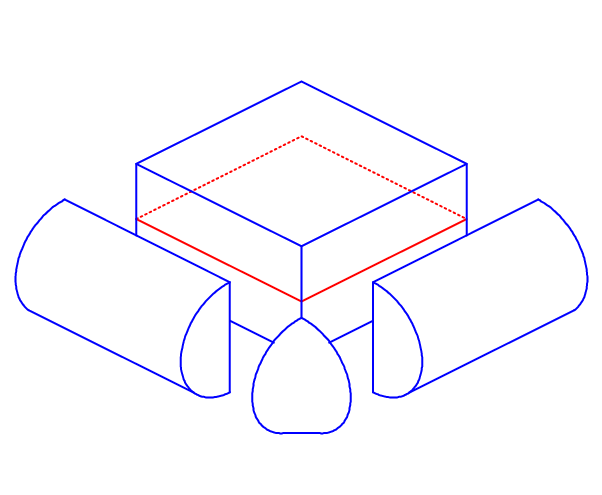
A version of the tube formula, without boundary corrections, was first derived by Weyl, 1939. Naiman, 1990 provided boundary corrections. The result is a series with terms. The first four terms (for manifolds on the unit sphere) are
| Volume | ||||
The constants , and arise from the corresponding series for the half-tubes around the boundaries of the manifold. is the -dimensional volume of the boundaries (or the total length of the four edges in Figure 2). and are higher order terms representing boundary curvature.
and arise from the ‘corner wedges’ where two boundary faces meet. In figure 2, is the sum of the four wedge angles at each corner of the manifold.
arises for manifolds with , from the corners where three (or more) boundary faces meet.
2.1 Random Processes
In statistical applications, the fundamental use of the tube formula is to find (or at least approximate) the distribution of the maximum of certain random processes. As a simple example, consider the process
where is an -valued vector function, and is uniformly distributed over the unit sphere. Suppose that one is interested in finding
for some .
The inner product exceeds if, and only if, is sufficiently close to . Specifically,
Hence, if, and only if, , where . The probability (2.1) is therefore simply
In many statistical applications, one is interested in the distribution of the maximum of a Gaussian process,
where follows the standard multivariate normal distribution. To reduce this to the uniform process, one needs to condition on the length of the vector, and integrate over the conditional distribution; see Sun and Loader, 1994. The final result, up to fourth order, is
where denotes a chi-square random variable with degrees of freedom.
3 The libtube Library
The main computational problem in implementing results based on the tube formula is evaluation of the constants , , e.t.c. The libtube library implements the tube library up to fourth order terms. To use the library, one must first write a ‘manifold function’ defining the problem. libtube takes the manifold function as input, and uses numerical integration methods to compute the constants.
The library can be downloaded from http://www.herine.net/stat/libtube. The library is written in C, and can be compiled on Linux systems using
% make
% make install
to install the libraries in /usr/local/lib.
% cc -o nlreg nlreg.c -ltube -lmut -lm
The library (and the examples given in this paper) have been written and tested using the Gnu C compiler available in most Linux distributions. The C code should be compatible with most other compilers and operating systems.
3.1 Manifold Functions
Suppose the manifold is defined by a vector function mapping a -dimensional domain to the manifold in -dimensional space. The constants in the tube formula can be computed from and its derivatives, so in it’s simplest form, the manifold function simply computes these. In statistical applications, one usually doesn’t get naturally, but rather one gets a vector such that (see the regression examples in Sections 4 and 5). The manifold function can instead provide and its derivatives.
In still other examples, one doesn’t even obtain directly, but instead obtains a covariance function (see the mixture example, Section 6). Since the distance between any two points on the manifold is given by
knowledge of the covariance function determines up to an orthogonal transformation. The manifold function can provide and its derivatives.
The precise form of the manifold functions is illustrated by the examples. After writing the manifold function, the most useful functions in libtube are:
- •
tube_contstants(), to numerically evaluate and the other constants appearing in (). - •
tailp()andcritval(), which compute tail probabilities corresponding to a specified cut-off, and critical values corresponding to a specified significance level.
Calling sequence for tube_constants().
The function to compute the constants is
int tube_constants(f, d, n, ev, mg, fl, kap, wk, deb, uc);
int (*f)();
int d, n, ev, mg;
double *fl, *kap, *wk;
int deb, uc;
The arguments to this function are:
- •
f The manifold function to compute and its derivatives.
- •
d The dimension of the manifold.
- •
m The maximum length of the vectors. The argument provided is only used to allocate work space; the actual length of is returned by the manifold function.
- •
ev Integration type. For rectangular domains, ISIMPSON is the most useful.
- •
mg Integer vector, giving the number of partitions to use in each dimension of the numerical integration rules.
- •
fl Integration limits. A numeric vector with length . The first components give lower limits for each variable; the remaining components give upper limits.
- •
kap is the vector through which the computed constants are returned. It should be allocated with at least terms. The values returned are and .
- •
wk is a workspace vector. If wk=NULL, the required workspace will be allocated and freed within the
tube_constants()function. To pre-allocate the space, the required length can be found by callingk0_reqd(d,m). - •
terms Number of terms to compute, from 1 to 4.
- •
uc An indicator variable indicating whether the manifold function computes the weight vectors uc=0 or covariance derivative matrix uc=1.
Calling sequence for tailp()
and critval().
Tail probabilities are computed using the function tailp:
double tailp(c,k0,m,d,s,n,process)
double c, *k0, n;
int m, d, s, process;
Critical values corresponding to a specified tail probability are computed using the critval function:
double critval(alpha,k0,m,d,s,n,process)
double *k0, al, n;
int m, d, it, s;
These arguments represent:
- •
c Cut-off value for
tailp(). - •
alpha tail probability for
critval(). - •
k0 is the vector of constants computed by the
tube_constants()function. - •
m is the number of terms in k0. This is the returned value of
tube_constants(), and is equal to . - •
d is the dimension of the manifold.
- •
c critical value (tailp() only).
- •
s Either
ONE_SIDEDorTWO_SIDED. - •
n For the t-process, the residual degrees of freedom used to estimate . For the uniform process, the dimension . Ignored for the Gaussian process. Beware that must have type double.
- •
process Either GAUSS (when is multivariate Gaussian); TPROC (Gaussian process with estimated variance); or UNIF (when is uniform on the unit sphere).
3.2 Writing a Manifold Function with vectors
The manifold function computes the vector and its derivatives. The basic form of the function is
int mymf(x,l,reqd)
double *x, *l;
int reqd;
{ /* function body goes here */
}
The x argument is a point in the input space; l is a vector to be filled in by the manifold function. The final argument, reqd, is an integer indicating what the library requires from the manifold function. If reqd=0, only the vector is required. If reqd=1, then both and (or all the first-order partial derivative vectors of ) are required. If reqd=2, then additionally the second-order partial derivative vectors are required.
In statistical applications, the manifold function will generally require a data vector, sample size , dimension and variables other than in order to perform its calculations. These variables should be assigned to global variables so that they are accessible in the manifold function.
The results of the computations are returned through the l vector. The vector is placed in the first elements. The first-order derivatives are placed in the next elements. The second-order derivatives are placed in the next elements.
The function should return , the length of the vector .
Generally, this should be equal to the value provided in the
tube_constants() call; it should never be larger. It
can be less. An example where it may be less is for a kernel regression
with compactly supported kernel; only the non-zero elements of
need be retained.
3.3 Writing a Manifold Function with a covariance function.
The structure of a manifold function based on the covariance is identical to the vector case; it differs in what is computed.
Given a covariance function , the manifold function needs to compute (in the one-dimensional case),
evaluated at . Again, the matrix is stored in the vector l, with the columns stacked atop each other.
In higher dimensions, the required matrix is most easily written in terms of differential operators. The required matrix is
where represents the partial derivative operator with respect to the subscripted variables.
Another view is as follows. If is the matrix computed by a manifold function with vectors, then is the matrix computed by a manifold function with a covariance function.
4 Example: Testing in Nonlinear Regression
This was the motivating example for Hotelling, 1939, and was developed in much more detail by Knowles and Siegmund, 1989. Suppose one has data , and a nonlinear regression model, such as
| (1) |
The important feature of this model is that the parameter enters the model linearly, while enters nonlinearly. Assume that the errors are independent .
Consider the problem of testing vs . It can be shown that the log-likelihood ratio test statistic is equivalent to
| (2) |
where .
In classical statistical theory, log-likeliood ratio statistics often have asymptotic distributions. However, this is not the case for the statistic (2). One way to see this is to recall that proofs of the results are based on a quadratic expansion of the statistic under the null parameters. For the present problem this would require an expansion around where is ‘the’ null value of . Unfortunately this is undefined: when , the parameter does not appear in (1); it is not identifiable!
For fixed , minimizing over is a linear least-sqaures problem. It follows that
The null hypothesis is rejected if for some , or equivalently, if
The constant must be chosen to obtain a specified significance level. That is, we need to be able to evaluate probabilities of the form
| (3) |
where defines a curve on the unit sphere, and is (under ) uniformly distributed on the surface of the sphere.
4.1 Non-linear Regression: Implementation
Code implementing the tube formla for the non-linear regression problem is shown below. The program consists of the manifold function regmf(), and the main routine main() that reads in the data and computes the tube constants. Note that the data vectors and sample size are stored as global variables, so that they can be accessed within the manifold function.
The manifold function computes the components of ; , and of , . These vectors are stored end-to-end in the l argument.
#include <stdio.h>
#include <math.h>
#include <tube.h>
#define MAXN 1000

double x[MAXN], y[MAXN];
int n;

int regmf(gam,l,reqd)
double *gam, *l;
int reqd;
{ int i;
  double *l1;
  l1 = &l[n];
  for (i=0; i<n; i++)
  { l[i] = exp(gam[0]*x[i]);
    l1[i] = x[i]*exp(gam[0]*x[i]);
  }
  return(n);
}

int main()
{ FILE *infile;
  char filename[100];
  int i, mg;
  double gamlimits[2], kappa[4];
  printf("Data filename ? "); scanf("%s",filename);
  printf("n = ? "); scanf("%d",&n);
  infile = fopen(filename,"r");
  for (i=0; i<n; i++) fscanf(infile,"%lf%lf",&x[i],&y[i]);
  gamlimits[0] = -2.0;
  gamlimits[1] = 2.0;
  mg = 100;

  tube_constants(regmf,1,n,ISIMPSON,&mg,gamlimits,kappa,NULL,0,0);
  printf("%8.5f %8.5f\n",kappa[0],kappa[1]);
}
5 Example: Simultaneous Confidence Bands
Application of the tube formula to find simultaneous confidence bands for regression models has been studied in Naiman, 1987, Sun and Loader, 1994 among others. Consider again regression data, but now suppose that the model is
(although we formulate the problem for quadratic regression, extension to other linear models is straightforward). The goal is to find confidence bands
with simultaneous coverage over some nice domain :
| (4) |
The least-squares estimates of the parameters are
where is the design matrix. For fixed , is estimated by
and the variance of the estimate is .
Now, , and the probability (4) is equivalent to
This problem can be solved using the Gaussian process variant of the tube problem.
Suppose is the -decomposition of the design matrix. Then lies in the column space of for all , and so
so it suffices to work with the vector where is a vector of the polynomial basis functions. The derivatives are easily found;
and so on.
5.1 Simultaneous Confidence Bands: Implementation
Code for the quadratic regression computations, in an arbitrary
number of dimensions, is shown below.
The functions quad(), quadi() and quadij()
compute the quadratic basis functions ; first-order partial
derivatives and second-order partial derivatives respectively.
The manifold function is quadmf(). The main()
function reads the data from a file; computes the design matrix
and its QR-decomposition; and then calls the
tube_constants() function (The QR functions,
qr() and qrtinvx(), as well as transpose(),
are part of the mut library).
When the program is run, the user is prompted for a data file (containing a matrix of the predictor variables); data dimension ( and ), and limits for the confidence band computation.
The tube constants are computed, then the critical value for 95% confidence bands. Note that the final argument to critval is the residual degrees of freedom used to estimate ; Sun and Loader, 1994 give the modification of () for this case.
#include <stdio.h>
#include <tube.h>
#include <mutil.h>

int dim, n, p;
double *X;

void quad(x,f)
double *x, *f;
{ int i, j, k;
  k = 0;
  f[k++] = 1.0;
  for (i=0; i<dim; i++) f[k++] = x[i];
  for (i=0; i<dim; i++)
    for (j=i; j<dim; j++)
      f[k++] = x[i]*x[j];
}

void quadi(x,f,i0)
double *x, *f;
int i0;
{ int i, j, k;
  k = 0;
  f[k++] = 0.0;
  for (i=0; i<dim; i++) f[k++] = (i==i0);
  for (i=0; i<dim; i++)
    for (j=i; j<dim; j++)
      f[k++] = (i==i0)*x[j] + (j==i0)*x[i];
}

void quadij(x,f,i0,j0)
double *x, *f;
int i0, j0;
{ int i, j, k;
  k = 0;
  f[k++] = 0.0;
  for (i=0; i<dim; i++) f[k++] = 0.0;
  for (i=0; i<dim; i++)
    for (j=i; j<dim; j++)
      f[k++] = ((i==i0) & (j==j0)) + ((i==j0) & (j==i0));
}

int quadmf(x,l,reqd)
double *x, *l;
int reqd;
{ int i, j, k;
  k = 0;
  quad(x,l);
  qrtinvx(X,l,n,p);
  k++;
  for (i=0; i<dim; i++)
  { quadi(x,&l[k*p],i);
    qrtinvx(X,&l[k*p],n,p);
    k++;
  }
  for (i=0; i<dim; i++)
    for (j=0; j<dim; j++)
    { quadij(x,&l[k*p],i,j);
      qrtinvx(X,&l[k*p],n,p);
      k++;
    }
  return(p);
}

int main()
{ FILE *infile;
  char filename[100];
  int i, j, mg[100];
  double xlim[100], kappa[4], datarow[100];
  printf("Data filename ? "); scanf("%s",filename);
  printf("n = ? "); scanf("%d",&n);
  printf("dim = ? "); scanf("%d",&dim);
  infile = fopen(filename,"r");
  if (infile==NULL)
  { printf("Error: can’t read input file\n");
    return(0);
  }
  p = 1 + dim + dim*(dim+1)/2;
  X = (double *)calloc(n*p,sizeof(double));
  for (i=0; i<n; i++)
  { for (j=0; j<dim; j++)
      fscanf(infile,"%lf",&datarow[j]);
    quad(datarow,&X[i*p]);
  }
  transpose(X,n,p);
  qr(X,n,p,NULL);
  for (i=0; i<dim; i++) mg[i] = 20;
  xlim[0] = -2; xlim[1] = -2;
  xlim[2] = 2; xlim[3] = 2;
  tube_constants(quadmf,dim,p,ISIMPSON,mg,xlim,kappa,NULL,3,0);
  printf("kappa: %8.5f %8.5f %8.5f %8.5f\n",kappa[0],kappa[1],kappa[2],kappa[3]);
}
6 Example: Mixture Models
Suppose are an i.i.d. sample from a density
where and are unknown parameters, with . The object is to test vs . This is a simple example of mixture testing: under , the single component describes the data, while under , the two components are required.
Consider the normalized score process proposed by Pilla and Loader, 2003. The score process is
Under the null hypothesis, this has mean 0 and covariance function , where
The normalized score process is . This asymptotically behaves like a Gaussian process , with mean 0 under , and a nonzero mean under . The maximum of the normalized score process serves as the test statistic.
Since an explicit vector representation of is not readily available, the manifold function (mixmf in the code below) must be written using the covariance function and its partial derivatives.
There is one additional difficulty. The normalized score process has a singularity at . For this reason, the manifold function works with Taylor series expansions of the covariance in this reason. Also, the singularity results in a discontinuity in , and .
The main routine in the program below sets limits for , calls the
tube_constants() function, and computes the 5% critical value.
kappa0 =  5.27449
  l0/2 =  2.00000
Level 0.05 critical value =  2.49455
#include <stdio.h>
#include <math.h>
#include <tube.h>
#define MAXN 1000

double x[MAXN], y[MAXN];
int n;

int mixmf(mu,l,reqd)
double *mu, *l;
int reqd;
{ double emm, mm;

  if (fabs(mu[0]) < 0.01)
  { mm = mu[0]*mu[0];
    l[0] = 1 + mm/2*(1 + mm/3*(1 + mm/4*(1 + mm/5)));
    l[1] = 0.5*(1 + mm/3*(2 + mm/4*(3 + mm/5*(4 + 5/6*mm))));
    l[1] = l[2] = mu[0]*l[1];
    l[3] = 0.5*(1 + mm/3*(4 + mm/4*(9 + mm/5*(16+25/6*mm))));
  } else
  { emm = exp(mu[0]*mu[0]);
    l[0] = emm-1;
    l[1] = l[2] = mu[0]*emm;
    l[3] = emm*(1+mu[0]*mu[0]);
  }
  return(2);
}

int main()
{ int i, mg, t;
  double mulimits[2], kappa[4];
  mulimits[0] = -3.0;
  mulimits[1] = 3.0;
  mg = 200;

  t = tube_constants(mixmf,1,n,ISIMPSON,&mg,mulimits,kappa,NULL,2,1);
  /* modify kappa[1] = l0/2 for the singularity */
  kappa[1] += 1.0;

  printf("kappa0 = %8.5f\n",kappa[0]);
  printf("  l0/2 = %8.5f\n",kappa[1]);
  printf("Level 0.05 critical value = %8.5f\n",critval(kappa,t,1,0.05,10,1,0.0));
}
References
- Hotelling, (1939) Hotelling, H. (1939). Tubes and spheres in -spaces, and a class of statistical problems. American Journal of Mathematics, 61:440–460.
- Knowles and Siegmund, (1989) Knowles, M. and Siegmund, D. (1989). On Hotelling’s geometric approach to testing for a nonlinear parameter in regression. International Statistical Review, 57:205–220.
- Naiman, (1987) Naiman, D. Q. (1987). Simultaneous confidence bounds in multiple regression using predictor variable constraints. Journal of the American Statistical Association, 82:214–219.
- Naiman, (1990) Naiman, D. Q. (1990). On volumes of tubular neighborhoods of spherical polyhedra and statistical inference. The Annals of Statistics, 18:685–716.
- Pilla and Loader, (2003) Pilla, R. S. and Loader, C. (2003). The volume-of-tube formula: Perturbation tests, mixture models and scan statistics. Unpublished Manuscript.
- Sun and Loader, (1994) Sun, J. and Loader, C. (1994). Simultaneous confidence bands for linear regression and smoothing. The Annals of Statistics, 22:1328–1345.
- Weyl, (1939) Weyl, H. (1939). On the volume of tubes. American Journal of Mathematics, 61:461–472.