Counting d -polytopes with + d 3 vertices

1 Introduction

A polytope $P$ is the convex hull of a finite set of point of a vector space $\mathbf{R}^{d}$ . If $P$ is not contained in any hyperplane of $\mathbf{R}^{d}$ , then $P$ is said $d$ -dimensional, or is called a $d$ -polytope. A vertex (resp. a facet) of $P$ is defined as the intersection of $P$ with an hyperplane $H$ of $\mathbf{R}^{d}$ such that $P\cap H$ has dimension $0$ (resp. has dimension $d-1$ ) and one of the two open sides of $H$ does not meet $P$ . A vertex $v$ is incident to a facet $f$ if $v\in f$ .

This article addresses the problem of counting combinatorially different $d$ -polytopes with $d+3$ vertices, meaning that two polytopes are identified if their incidences vertices-facets are isomorphic (i.e. the incidences are the same up to relabeling of the vertices). Whereas general $d$ -polytopes are involved objects, $d$ -polytopes with few vertices are combinatorially tractable. Precisely, each combinatorial $d$ -polytope with $d+3$ vertices gives rise in a bijective way to a configuration of $d+3$ points in the plane, placed at the centre and at vertices of a regular $2k$ -gon, and satisfying two local conditions and a global condition. As a consequence, counting combinatorial $d$ -polytopes with $d+3$ vertices boils down to the much easier task of counting such configurations of $d+3$ points, called reduced Gale diagrams. Following this approach, Perles [2, p. 113] gave an explicit formula for the number of (combinatorial) simplicial $d$ -polytopes with $d+3$ vertices and Lloyd [3] gave a more complicated formula for $c(d+3,d)$ the number of combinatorial $d$ -polytopes with $d+3$ vertices. However, as pointed out in the new edition of Grünbaum’s book [2, p. 121a], Lloyd’s formula does not match with the first values of $c(d+3,d)$ , obtained by Perles [2, p. 424].

In this article, we both correct the mistake of Lloyd and propose a more complete and self-contained solution for this enumeration problem. The following theorem is our main result:

Theorem 1

Let $c(d+3,d)$ be the number of combinatorially different $d$ -polytopes with $d+3$ vertices. Then the generating function $\displaystyle P(x)=\sum_{d}c(d+3,d)x^{d+3}$ has the following expression, where $\phi(.)$ is the Euler totient function:

P(x)=-\frac{1}{1-x}\sum_{e\ odd}\frac{\phi(e)}{4e}\ln\left(1-\frac{2x^{3e}}{(1-2x)^{2e}}\right)+\frac{1}{1-x}\sum_{e\geq 1}\frac{\phi(e)}{2e}\ln\left(\frac{1-x^{e}}{1-2x^{e}}\right)\\ +{\frac{x\left({x}^{2}-x-1\right)\left({x}^{4}-{x}^{2}+1\right)}{2\left(1-x\right)^{2}\left(2\,{x}^{6}-4\,{x}^{4}+4\,{x}^{2}-1\right)}}-{\frac{x\left({x}^{8}-2\,{x}^{7}+{x}^{6}+3\,{x}^{3}-{x}^{2}-x+1\right)}{\left(1+x\right)^{2}\left(1-x\right)^{6}}}

(1)

The first terms of the series are $P(x)=x^{5}+7x^{6}+31x^{7}+116x^{8}+379x^{9}+1133x^{10}+3210x^{11}+\ldots$ , i.e. there is one polytope with 5 vertices in the plane (the pentagon), there are 7 polytopes with 6 vertices in the 3-D space, etc.

The mistake of Lloyd, pointed precisely in Section 5, is in the last rational term of $P(x)$ . Lloyd derived from his expression of $P(x)$ an explicit formula for $c(d+3,d)$ , which does not match with the correct values of $c(d+3,d)$ because of the mistake in the computation of $P(x)$ . We do not perform such a derivation for two reasons: first, several equivalent formulas for $c(d+3,d)$ can be derived from the expression of $P(x)$ , so that the canonical form seems to be on the generating function rather than on the coefficients. Second, explicit formulas for $c(d+3,d)$ such as the one of Lloyd involve double summations, hence require a quadratic number of arithmetic operations to compute $c(d+3,d)$ . As opposed to that and discussed in Section 8, the coefficients $c(d+3,d)$ can be directly extracted iteratively from the expression of $P(x)$ in a very efficient way: a table of the $N$ first coefficients can be computed with $\mathcal{O}(N\log(N))$ operations. Using a mathematical software like Maple, a table of several hundreds of coefficients can easily be obtained.

In Section 7, we introduce the problem of counting oriented $d$ -polytopes with $d+3$ vertices, meaning that two polytopes are equivalent if they have the same combinatorial structure and there exists an orientation-preserving of $\mathbf{R}^{d}$ homeomorphism mapping the first one to the second one. We establish a bijection between oriented $d$ -polytopes with $d+3$ vertices and so-called oriented reduced Gale diagrams of size $d+3$ , adapting the original bijection so as to take the orientation into account. To our knowledge, this oriented version of the bijection was not stated before. The bijection implies that the task of counting oriented $d+3$ -vertex $d$ -polytopes reduces to the task of counting oriented reduced Gale diagrams with respect to the size, which is done in a similar way as the enumeration of Gale diagrams. As a corollary, we also enumerate combinatorial $d+3$ -vertex $d$ -polytopes giving rise to only one oriented polytope. These polytopes, called achiral, are also characterized as having a geometric representant fixed by a reflection of $\mathbf{R}^{d}$ .

Finally, in Section 9, we give precise asymptotic estimates for the coefficients $c(d+3,d)$ , $c^{+}(d+3,d)$ , $c^{-}(d+3,d)$ counting (combinatorial) $d$ -polytopes, oriented $d$ -polytopes and achiral $d$ -polytopes with $d+3$ vertices. No asymptotic result was given in Lloyd’s paper, but Perles [2, p.114] proved that there exist two constants $c_{1}$ and $c_{2}$ such that $c_{1}\frac{\gamma^{d}}{d}\leq c(d+3,d)\leq c_{2}\frac{\gamma^{d}}{d}$ , where $\gamma$ is explicit, $\gamma\approx 2.83$ . Using analytic combinatorics, we deduce from the expression of $P(x)$ that $c(d+3,d)\sim c\frac{\gamma^{d}}{d}$ , with $c$ an explicit constant and $\gamma$ equal to the $\gamma$ of Perles, but with a simplified definition. Hence this agrees with Perle’s estimate and refines it.

Overview of the proof of Theorem 1.

In Section 2.1, we give a sketch of proof of the bijection between combinatorial $(d+3)$ -vertex $d$ -polytopes and reduced Gale diagrams of size $d+3$ . With this bijection, the enumeration of $(d+3)$ -vertex $d$ -polytopes reduces to the enumeration of reduced Gale diagrams with respect to the size.

The scheme of our method of enumeration of reduced Gale diagrams follows, in a more detailed way, the same lines as Lloyd. The first observation (see Section 2.2) is that it is sufficient to concentrate on the enumeration of reduced Gale diagrams with no label at the centre and satisfying the two local conditions (forgetting temporarily the third global condition). We introduce a special terminology for these diagrams, calling them wheels. As wheels are enumerated up to rotation and up to reflection, they are subject to symmetries: Burnside’s lemma reduces the task of counting wheels to the task of counting so-called rooted wheels (where the presence of a root deletes possible symmetries) and rooted symmetric wheels of two types: rotation and reflection, see Section 3.

After these preliminaries, our treatment for the enumeration of rooted wheels differs from that of Lloyd, which relies on an auxiliary theorem of Read, requiring to operate in two steps. The method we propose in Section 4.1 is direct and self-contained: we associate with a rooted wheel a word on a specific (infinite) alphabet and we show that the set of words derived from rooted wheels is recognized by a simple automaton (see Figure 3(a)). Under the framework of automata, generating functions appear as a very powerful tool providing simple (in general rational) and compact solutions in an automatic way. We derive from the automaton an explicit rational expression for the generating function of rooted wheels. The enumeration of rooted symmetric wheels is done in a similar way, associating words with such rooted wheels and observing that the obtained sets of words are recognized by automata. The injection into Burnside’s Lemma of the rational expressions for rooted and rooted symmetric wheels yields an explicit expression for the generating functions of wheels, given in Section 4.4. Theorem 1 follows after taking the global condition (called half-plane condition) into account, which requires only some exhaustive treatment of cases, see Section 5.

2 Gale diagrams of $(d+3)$ -vertex $d$ -polytopes

2.1 Gale diagrams

Following Perles and Lloyd, we define a reduced Gale diagram as a regular $2k$ -gon, with $k\geq 2$ , that carries non-negative labels at its centre and at its vertices, with the following properties:

P1:: Two opposite vertices of the $2k$ -gon cannot both have label 0
P2:: Two neighbour vertices of the $2k$ -gon cannot both have label 0
P3:: (half-plane condition) Given any diameter of the $2k$ -gon, the sum of the labels of vertices belonging to any (open) side of the diameter is at least 2.

In addition, two reduced Gale diagrams are identified if the first one can be obtained from the second one by a rotation or by a rotation and a reflection. The size of a reduced Gale diagram is defined as the sum of its labels. The following theorem is essential in order to reduce the problem of enumeration of polytopes to the tractable problem of counting reduced Gale diagrams. Details of the proof can be found in Grünbaum’s book [2, Sect. 6.3].

Theorem 2

(Perles) The number of combinatorially different $d$ -polytopes with $d+3$ vertices is equal to the number of reduced Gale diagrams of size $d+3$ .

Proof (Sketch): Given a $d$ -polytope $P$ with $d+3$ vertices $v_{1},\ldots,v_{d+3}$ , a matrix $M_{P}$ is associated with $P$ in the following way: $M_{P}$ has $d+3$ rows, the $i$ th row consisting of a 1 followed by the $d$ -vector-position of the vertex $v_{i}$ . Hence, $M_{P}$ has $d+1$ columns, and it can be shown that $M_{P}$ has rank $d+1$ . As a consequence, the vector space $\mathcal{V}(P)$ spanned by the column vectors $(C_{1},\ldots,C_{d+1})$ of $M_{P}$ has dimension $d+1$ , so its orthogonal $\mathcal{V}(P)^{\bot}$ has dimension 2. Let $(A_{1},A_{2})$ be a base of $\mathcal{V}(P)^{\bot}$ and let $A$ be the $(d+3)\times 2$ matrix whose two columns are $(A_{1},A_{2})$ . Then $A$ is called a Gale diagram of $P$ . The matrix $A$ can be seen as a configuration of $d+3$ points in the plane, each point corresponding to a row of $A$ . The combinatorial structure of $P$ , i.e. the incidences vertices-facets, can be recovered from $A$ . However, several Gale diagrams can correspond to the same (combinatorial) polytope. One can perform successive reductions, keeping the same associated combinatorial polytope, so that the $d+3$ points of the diagram are finally located either at the centre or at vertices of a regular $2k$ -gon. Giving to the centre and to each vertex of the $2k$ -gon a label indicating the number of points located at it, one obtains a $2k$ -gon with labels characterized by the fact that they satisfy properties P1, P2 and P3. In addition, it can be shown that this reduction is maximal, i.e. that the combinatorial types of the polytopes associated with two inequivalent (i.e. not equal up to rotation and reflection) reduced Gale diagrams are different. $\Box$

2.2 Gale diagrams and wheels

A first remark is that properties P1, P2, P3 do not depend on the value of the label at the centre of the $2k$ -gon. Hence the number $g_{n}$ of reduced Gale diagrams of size $n$ is easily deduced from the coefficients $e_{i}$ counting reduced Gale diagrams of size $i$ with label 0 at the centre (such reduced Gale diagrams correspond to so-called non-pyramidal polytopes):

g_{n}=\sum_{i=1}^{n}e_{i}.

As a consequence, we concentrate on the enumeration of labelled $2k$ -gons (meaning that only the $2k$ vertices of the $2k$ -gon carry labels) satisfying properties P1, P2, P3.

A second remark is that Property P3 is implied by Property P2 if the number of diameters is at least 5. As a consequence, we will first put aside Property P3 and focus on the enumeration of labelled $2k$ -gons satisfying properties P1 and P2 (counted up to rotation and up to reflections). Such labelled $2k$ -gons are called wheels. Wheels with 2 vertices, even though corresponding to a degenerated polygon, are also counted. The enumeration of wheels will be performed in Section 3 and Section 4. By definition of wheels, the number of reduced Gale diagrams with no label at the centre is obtained as the difference between the number of wheels and the number of wheels not satisfying Property P3. The latter term, considered in Section 5, is easy to calculate using some exhaustive treatment of cases, because wheels not satisfying Property P3 have at most 4 diameters.

3 Method of enumeration of wheels

3.1 Rooted wheels

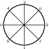
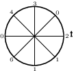
A wheel is rooted by selecting one vertex of the $2k$ -gon and by choosing a sense of traversal (clockwise or counter-clockwise) of the $2k$ -gon. See Figure 1(b) for an example ¹¹ 1 On the figures, regular $2k$ -gons are represented as $2k$ vertices regularly distributed on a circle, for aesthetic reasons and consistence with the terminology of wheels..

Traversing the $2k$ -gon from the selected vertex in the direction indicated by the root, one obtains an integer sequence $(a_{1},\ldots,a_{2k})$ satisfying the following conditions:

S1:: For each $1\leq i\leq 2k$ , $a_{i}$ and $a_{(i+k)\mod 2k}$ are not both $0$ .
S2:: For each $1\leq i\leq 2k$ , $a_{i}$ and $a_{(i+1)\mod 2k}$ are not both $0$ .

An integer sequence satisfying properties S1 and S2 is called a wheel-sequence. The size of the wheel-sequence is defined as $(a_{1}+\ldots+a_{2k})$ . Properties S1 and S2 are simply the respective transpositions of properties P1 and P2 on the integer sequence, so that we can identify rooted wheels with size $n$ and $k$ diameters and wheel-sequences of size $n$ and length $2k$ .

3.2 Burnside’s lemma

Burnside’s lemma is a convenient tool to enumerate objects defined modulo the action of a group, which means that they are counted modulo symmetries. Let $G$ be a finite group acting on a finite set $E$ . Given $g\in G$ , we write $\mathrm{Fix}_{g}$ for the set of elements of $E$ fixed by $g$ . Then the number of orbits of $E$ under the action of $G$ is given by:

|\mathrm{Orb}_{E}|=\frac{1}{|G|}\sum_{g\in G}|\mathrm{Fix}_{g}|

(2)

where $|.|$ stands for cardinality.

3.3 Burnside’s lemma applied to wheels

A wheel with size $n$ and $k$ diameters corresponds to an orbit of rooted wheels with size $n$ and $k$ diameters under the action of the dihedral group $D_{2k}$ . Equivalently, using the identification between rooted wheels and wheel-sequences, a wheel with size $n$ and $k$ diameters corresponds to an orbit of wheel-sequences of size $n$ and length $2k$ under the action of $D_{2k}=\mathbf{Z}_{2k}\times\{+,-\}$ , where the action is defined as follows, see Figure 2:

	$\displaystyle(l,+)\cdot(a_{1},\ldots,a_{2k})$	$\displaystyle=$	$\displaystyle(a_{1+l},\ldots,a_{2k},a_{1},\ldots,a_{l})$
	$\displaystyle(l,-)\cdot(a_{1},\ldots,a_{2k})$	$\displaystyle=$	$\displaystyle(a_{1+l},a_{l},\ldots,a_{1},a_{2k},\ldots,a_{2+l}),$

i.e. $(l,+)$ is a rotation and $(l,-)$ is a reflection.

Let us now introduce some definitions. A rotation-wheel is a pair made of a rooted wheel and of a rotation of order at least 2 fixing the rooted wheel. Equivalently, it is a pair made of a sequence $(a_{1},\ldots,a_{2k})$ and of an element $(l,+)$ with $l\neq 0$ such that $(l,+)\cdot(a_{1},\ldots,a_{2k})=(a_{1},\ldots,a_{2k})$ . A reflection-wheel is a pair made of a rooted wheel and of a reflection fixing the rooted wheel. Equivalently, it is a pair made of a sequence $(a_{1},\ldots,a_{2k})$ and of an element $(l,-)$ such that $(l,-)\cdot(a_{1},\ldots,a_{2k})=(a_{1},\ldots,a_{2k})$ . The following proposition ensures that, using Burnside’s formula, counting wheels reduces to counting rooted wheels, rotation wheels and reflection wheels.

Proposition 3

Let $W_{n,k}$ , $R_{n,k}$ , $R_{n,k}^{+}$ , $R_{n,k}^{-}$ be respectively the numbers of wheels, rooted wheels, rotation-wheels, and reflection-wheels with size $n$ and $k$ diameters. Let $W(x,u)$ , $R(x,u)$ , $R^{+}(x,u)$ , and $R^{-}(x,u)$ be their generating functions. Then

4u\frac{\partial W}{\partial u}(x,u)=R(x,u)+R^{+}(x,u)+R^{-}(x,u).

(3)

Proof: As wheels with $k$ diameters are orbits of rooted wheels with $k$ diameters under the action of the dihedral group $D_{2k}$ (which has cardinality $4k$ ), Burnside’s formula yields

W_{n,k}=\frac{1}{4k}\left(R_{n,k}+R_{n,k}^{+}+R_{n,k}^{-}\right).

Hence $\displaystyle\sum 4kW_{n,k}x^{n}u^{k}=\sum R_{n,k}x^{n}u^{k}+\sum R_{n,k}^{+}x^{n}u^{k}+\sum R_{n,k}^{-}x^{n}u^{k}$ , which yields (3). $\Box$

4 Enumeration of wheels

4.1 Enumeration of rooted wheels

In this section, we explain how to obtain a rational expression for the generating function $R(x,u)$ counting rooted wheels with respect to the size and number of diameters.

4.1.1 The word associated to a rooted wheel.

Let $s=(a_{1},\ldots,a_{2k})$ be a wheel-sequence of size $n$ and length $2k$ . Associate with $s$ the following word:

\sigma:=\binom{a_{1}}{a_{k+1}},\binom{a_{2}}{a_{k+2}},\ldots,\binom{a_{k}}{a_{2k}}

Observe that the length of $\sigma$ is the number of diameters of the associated rooted wheel. As each letter of $\sigma$ contains a pair of opposite vertices of the $2k$ -gon, the fact that two opposite vertices are not both 0 (Property P1 or equivalently Property S1) translates into the following property:

\sigma\mathrm{\ is\ a\ word\ on\ the\ alphabet}\ \mathcal{A}:=\mathbf{N}^{2}\backslash\left\{\binom{0}{0}\right\}.

Now let us detail the translation of Property P2 (or S2) on the word $\sigma$ . First, the alphabet $\mathcal{A}$ is partitioned into three subalphabets:

\mathcal{B}=\left\{\binom{i}{j}\ \mathrm{with}\ i>0,j>0\right\},\mathcal{C}=\left\{\binom{i}{0}\ \mathrm{with}\ i>0\right\},\mathcal{D}=\left\{\binom{0}{j}\ \mathrm{with}\ j>0\right\}

Property S2 is translated as follows:

•

$a_{i}$ and $a_{i+1}$ are not both $0$ for $1\leq i\leq k-1$ $\Longleftrightarrow$ $\sigma_{i}$ and $\sigma_{i+1}$ are not both in $\mathcal{D}$ for $1\leq i\leq k-1$
•

$a_{k+i}$ and $a_{k+i+1}$ are not both $0$ for $1\leq i\leq k-1$ $\Longleftrightarrow$ $\sigma_{i}$ and $\sigma_{i+1}$ are not both in $\mathcal{C}$ for $1\leq i\leq k-1$
•

$a_{k}$ and $a_{k+1}$ are not both $0$ $\Longleftrightarrow$ the pair $(\sigma_{1},\sigma_{k})$ is not in $\mathcal{C}\times\mathcal{D}$
•

$a_{1}$ and $a_{2k}$ are not both $0$ $\Longleftrightarrow$ the pair $(\sigma_{1},\sigma_{k})$ is not in $\mathcal{D}\times\mathcal{C}$

Hence $\sigma$ is characterized as a word on the alphabet $\mathcal{A}$ that contains no factor $\mathcal{C}\mathcal{C}$ nor factor $\mathcal{D}\mathcal{D}$ and such that the pair made of its first and last letter in not in $\mathcal{C}\times\mathcal{D}$ nor in $\mathcal{D}\times\mathcal{C}$ .

The size of a letter is defined as the sum of its two integers, and the size of the word $\sigma$ is defined as the sum of the sizes of its letters. Hence the size of a rooted wheel is equal to the size of its associated word.

Notice that the generating functions of the three subalphabets $\mathcal{B}$ , $\mathcal{C}$ , and $\mathcal{D}$ with respect to the size are:

B(x)=\left(\frac{x}{1-x}\right)^{2}\ \ \ C(x)=\frac{x}{1-x}\ \ \ D(x)=\frac{x}{1-x}

(4)

4.1.2 Generic automaton and its generating functions

First we explain how to enumerate the words on the alphabet $\mathcal{A}$ avoiding the factors $\mathcal{C}\mathcal{C}$ and $\mathcal{D}\mathcal{D}$ . The set of these words is recognized by the automaton represented on Figure 3(b), obtained from the automaton of Figure 3(a) by choosing $\{0\}$ as starting state (entering arrow) and $\{0,1,2\}$ as end-states (leaving arrows). We call the automaton of Figure 3(a) generic because rooted wheels, rotation-wheels and reflection-wheels will give rise to languages on $\mathcal{A}$ recognized by slight modifications of this automaton.

For $i\in\{0,1,2\}$ and $j\in\{0,1,2\}$ , we denote by $\mathcal{L}_{ij}$ the set of words accepted by the generic automaton that start at state $i$ and end at state $j$ . Let $L_{ij}(x,u)$ be the generating function of $\mathcal{L}_{ij}$ with respect to the size and length of the word. Looking at the starting state and first letter of a word recognized by the generic automaton and ending at $0$ , one gets the following system satisfied by the three generating functions $L_{00}(x,u)$ , $L_{10}(x,u)$ and $L_{20}(x,u)$ :

\displaystyle\left\{\begin{array}[]{rcl}L_{00}(x,u)&=&1+uB(x)L_{00}(x,u)+uC(x)L_{10}(x,u)+uD(x)L_{20}(x,u)\\ L_{10}(x,u)&=&uB(x)L_{00}(x,u)+uD(x)L_{20}(x,u)\\ L_{20}(x,u)&=&uB(x)L_{00}(x,u)+uC(x)L_{10}(x,u)\end{array}\right.

Replacing $B(x)$ , $C(x)$ and $D(x)$ by their expressions given in (4), this system becomes

\left(\begin{array}[]{c}L_{00}(x,u)\\ L_{10}(x,u)\\ L_{20}(x,u)\end{array}\right)=\left(\begin{array}[]{ccc}\frac{ux^{2}}{(1-x)^{2}}&\frac{ux}{1-x}&\frac{ux}{1-x}\\ \frac{ux^{2}}{(1-x)^{2}}&0&\frac{ux}{1-x}\\ \frac{ux^{2}}{(1-x)^{2}}&\frac{ux}{1-x}&0\end{array}\right)\cdot\left(\begin{array}[]{c}L_{00}(x,u)\\ L_{10}(x,u)\\ L_{20}(x,u)\end{array}\right)+\left(\begin{array}[]{c}1\\ 0\\ 0\end{array}\right).

Solving this matrix equation, one gets explicit rational expressions for $L_{00}(x,u)$ , $L_{10}(x,u)$ and $L_{20}(x,u)$ , for instance:

\displaystyle L_{10}(x,u)=\frac{ux^{2}(1-x)}{1-x(3+u-3x-ux+x^{2}+u^{2}x^{2})}.

One can similarly define a matrix-equation satisfied by $\{L_{01}(x,u),L_{11}(x,u),L_{21}(x,u)\}$ and a matrix-equation satisfied by $\{L_{02}(x,u),L_{12}(x,u),L_{22}(x,u)\}$ , from which one gets explicit rational expressions for these generating functions.

4.1.3 Expression of the generating function of rooted wheels

As we have seen in Section 3.1, rooted wheels with size $n$ and $k$ diameters can be identified with non-empty words of size $n$ and length $k$ on the alphabet $\mathcal{A}$ , avoiding the factors $\mathcal{C}\mathcal{C}$ and $\mathcal{D}\mathcal{D}$ and such that the pair made of their first and last letter is not in $\mathcal{C}\times\mathcal{D}$ nor in $\mathcal{D}\times\mathcal{C}$ .

The language of these words is recognized by the automaton represented on Figure 4. Hence the generating function $R(x,u)$ counting rooted wheels with respect to the size and number of diameters satisfies:

	$\displaystyle R(x,u)$	$\displaystyle=$	$\displaystyle uD(x)(L_{20}(x,u)+L_{22}(x,u))+uC(x)(L_{11}(x,u)+L_{10}(x,u))$
			$\displaystyle+uB(x)(L_{00}(x,u)+L_{01}(x,u)+L_{02}(x,u))$

Replacing the generating functions on the right hand side by their rational expressions yields

R(x,u)={\frac{ux\left({u}^{2}{x}^{3}-2\,u{x}^{3}+2\,u{x}^{2}-{x}^{3}+4\,{x}^{2}-5\,x+2\right)}{\left({u}^{2}{x}^{3}-u{x}^{2}-3\,{x}^{2}+{x}^{3}+3\,x+ux-1\right)\left(x-ux-1\right)}}.

(5)

4.2 Enumeration of rotation-wheels

As follows from the definition of rotation-wheels and from the identification between rooted wheels and wheel-sequences, a rotation-wheel corresponds to a pair made of a wheel-sequence $s=(a_{1},\ldots,a_{2k})$ and of an element $l\in\mathbf{Z}_{2k}\backslash\{0\}$ such that the sequence $s$ is equal to its $l$ -shift. Writing $e$ for the order of $l$ in $\mathbf{Z}_{2k}$ (hence $e$ divides $2k$ ), the sequence $s$ is characterized by the property that it can be written as $e$ concatenated copies of an integer sequence $(\alpha_{1},\ldots,\alpha_{2k/e})$ . In addition, it is well-known that for each divisor $e$ of $2k$ there are exactly $\phi(e)$ elements $l$ of order $e$ in $\mathbf{Z}_{2k}$ . This yields the following lemma:

Lemma 4

Let $\mathcal{R}^{(e)}$ be the set of rooted wheels whose wheel-sequence can be written as $e$ concatenated copies of an integer-sequence. Let $R^{(e)}(x,u)$ be the generating function of $\mathcal{R}^{(e)}$ with respect to the size and number of diameters. Then the generating function $R^{+}(x,u)$ of rotation-wheels is:

R^{+}(x,u)=\sum_{e\geq 2}\phi(e)R^{(e)}(x,u)

(6)

Let $e\geq 2$ and consider a rooted wheel of $\mathcal{R}^{(e)}$ , so that its associated sequence $(a_{1},\ldots,a_{2k})$ consists of $e$ concatenated copies of an integer sequence $\alpha=(\alpha_{1},\ldots,\alpha_{2k/e})$ . We give a combinatorial characterization of the sequence $\alpha$ by distinguishing two cases:

The number $e$ of copies is even.

In this case, the opposite vertex of $\alpha_{i}$ on the $2k$ -gon is $\alpha_{i}$ , see Figure 5(a). As two opposite vertices of a wheel can not both have label 0 (Property P1), all integers $\alpha_{i}$ have to be positive. This condition ensures that two neighbour vertices of the $2k$ -gon are not both 0 (Property P2). Hence, for $r\geq 1$ , a rooted wheel of $\mathcal{R}^{(2r)}$ with size $n$ and $k$ diameters corresponds to $2r$ concatenated copies of a non-empty sequence of positive integers of size $n/(2r)$ and length $k/r$ . The generating function $I(x,u)$ counting non-empty sequences of positive integers with respect to the size and length is:

I(x,u)=u\frac{x}{1-x}\frac{1}{1-u\frac{x}{1-x}}=\frac{ux}{1-x(1+u)}.

Hence we obtain:

R^{(2r)}(x,u)=I(x^{2r},u^{r})=\frac{u^{r}x^{2r}}{1-x^{2r}(1+u^{r})}.

(7)

The number $e$ of copies is odd.

As $e$ is odd and divides $2k$ , it also divides $k$ . Hence $k/e$ is an integer, that we denote by $k^{\prime}$ . In this case, for $1\leq i\leq 2k^{\prime}$ , the opposite vertex of $\alpha_{i}$ on the $2k$ -gon is $\alpha_{(i+k^{\prime})\mod 2k^{\prime}}$ , see Figure 5(b). In addition, for $1\leq i\leq 2k^{\prime}$ , the next neighbour of $\alpha_{i}$ on the $2k$ -gon is $\alpha_{(i+1)\mod 2k^{\prime}}$ . As a consequence, the fact that $(a_{1},\ldots,a_{2k})$ is a wheel-sequence is equivalent to the fact that $(\alpha_{1},\ldots,\alpha_{2k^{\prime}})$ is a wheel-sequence. Thus a wheel-sequence associated with a rooted wheel of $\mathcal{R}^{(2r+1)}$ corresponds to $(2r+1)$ concatenated copies of a wheel-sequence, so that for $r\geq 1$ :

R^{(2r+1)}(x,u)=R(x^{2r+1},u^{2r+1}),

(8)

where $R(x,u)$ is the generating function of rooted wheels.

Finally, equations (6), (7) and (8) yield the following explicit expression of the generating function of rotation-wheels:

R^{+}(x,u)=\sum_{r\geq 1}\phi(2r+1)R(x^{2r+1},u^{2r+1})+\sum_{r\geq 1}\phi(2r)\frac{u^{r}x^{2r}}{1-x^{2r}(1+u^{r})}

(9)

4.3 Enumeration of reflection-wheels

We recall that a reflection-wheel is a pair made of a rooted wheel and of a reflection fixing it. It can also be seen as a pair made of a wheel-sequence $(a_{1},\ldots,a_{2k})$ and of an element $l\in\mathbf{Z}_{2k}$ such that $(a_{1},\ldots,a_{2k})=(a_{1+l},a_{l},\ldots,a_{1},a_{2k},\ldots,a_{2+l})$

Lemma 5

Let $R^{(-1,-)}(x,u)$ be the generating function of rooted wheels fixed by the reflection $(-1,-)$ and let $R^{(0,-)}(x,u)$ be the generating function of rooted wheels fixed by the reflection $(0,-)$ . Then the generating function $R^{-}(x,u)$ of reflection-wheels is:

R^{-}(x,u)=u\frac{\partial}{\partial u}\left(R^{(-1,-)}(x,u)+R^{(0,-)}(x,u)\right).

(10)

Proof: For $k\geq 1$ and $l\in\mathbf{Z}_{2k}$ , we denote by $\mathcal{R}_{n,k}^{(l,-)}$ the set of rooted wheels with size $n$ and $k$ diameters whose associated sequence verifies $(a_{1},\ldots,a_{2k})=(a_{1+l},a_{l},\ldots,a_{1},a_{2k},\ldots,a_{2+l})$ . By definition, the set $\mathcal{R}_{n,k}^{-}$ of reflection-wheels with size $n$ and $k$ diameters is given by $\mathcal{R}_{n,k}^{-}=\cup_{l=0}^{2k-1}\mathcal{R}_{n,k}^{(l,-)}$ . Observe that if a wheel sequence is fixed by the action of $(l,-)$ , then its $r$ -shift is fixed by the action of $(l-2r,-)$ . As a consequence, $\mathcal{R}_{n,k}^{(l,-)}$ is in bijection with $\mathcal{R}_{n,k}^{(0,-)}$ if $l$ is even (these cases are those of a reflection fixing two vertices of the $2k$ -gon); and $\mathcal{R}_{n,k}^{(l,-)}$ is in bijection with $\mathcal{R}_{n,k}^{(-1,-)}$ if $l$ is odd (these cases are those of a reflection fixing no vertex of the $2k$ -gon). This directly yields $|\mathcal{R}_{n,k}^{-}|=k\left(|\mathcal{R}_{n,k}^{(0,-)}|+|\mathcal{R}_{n,k}^{(-1,-)}|\right)$ , from which Equation (10) follows. $\Box$

4.3.1 Enumeration of rooted wheels fixed by the reflection $(0,-)$

Let $(a_{1},\ldots,a_{2k})$ be a wheel-sequence fixed by $(0,-)$ . Then $(a_{1},\ldots,a_{2k})$ can be written as $(\beta,\alpha_{1},\ldots,\alpha_{k-1},\gamma,\alpha_{k-1},\ldots,\alpha_{1})$ , see Figure 6(a). Observe that $\beta$ is opposite to $\gamma$ and that, for $1\leq i\leq k-1$ , $\alpha_{i}$ is opposite to $\alpha_{k-i}$ on the $2k$ -gon. Then two cases arise:

The number of diameters is odd.

In this case, we write $r$ for the integer $(k-1)/2$ . Then the fact that two opposite vertices of the rooted wheel do not both have label 0 (Property P1) is equivalent to the fact that:

\sigma:=\binom{\beta}{\gamma},\binom{\alpha_{1}}{\alpha_{2r}},\ldots,\binom{\alpha_{r}}{\alpha_{r+1}}

is a word on the alphabet $\mathcal{A}:=\mathbf{N}^{2}\backslash\{\binom{0}{0}\}$ .

In addition, Property P2 (two neighbours can not both have label 0) translates as follows:

•

$\beta$ and $\alpha_{1}$ are not both 0 and $\alpha_{i}$ and $\alpha_{i+1}$ are not both 0 for $1\leq i\leq r-1$ $\Longleftrightarrow$ $\sigma$ contains no factor $\mathcal{D}\mathcal{D}$ .
•

$\gamma$ and $\alpha_{2r}$ are not both 0 and $\alpha_{i}$ and $\alpha_{i+1}$ are not both 0 for $r+1\leq i\leq 2r-1$ $\Longleftrightarrow$ $\sigma$ contains no factor $\mathcal{C}\mathcal{C}$ .
•

$\alpha_{r}$ and $\alpha_{r+1}$ are not both 0 $\Longleftrightarrow$ the last letter of $\sigma$ is in the alphabet $\mathcal{A}$ (already implied by Property P1)

Hence $\sigma$ is characterized as a non-empty word on the alphabet $\mathcal{A}$ that contains no factor $\mathcal{C}\mathcal{C}$ nor factor $\mathcal{D}\mathcal{D}$ . The set of words on $\mathcal{A}$ satisfying this last property is already recognized by the automaton represented on Figure 3(b). However, the first letter of $\sigma$ , containing the two fixed points, counts once in the sequence $(a_{1},\ldots,a_{2k})$ , whereas the other letters count twice. Hence we rather use the automaton of Figure 7, which recognizes non-empty words avoiding $\mathcal{C}\mathcal{C}$ and $\mathcal{D}\mathcal{D}$ , and where the first letter of the word is read separately. From this automaton, we get the generating function $R_{odd}^{(0,-)}(x,u)$ of rooted wheels fixed by $(0,-)$ and with an odd number of diameters:

$\displaystyle R_{odd}^{(0,-)}(x,u)$	$\displaystyle=$	$\displaystyle uB(x)(L_{00}(x^{2},u^{2})+L_{01}(x^{2},u^{2})+L_{02}(x^{2},u^{2}))$
		$\displaystyle+uC(x)(L_{10}(x^{2},u^{2})+L_{11}(x^{2},u^{2})+L_{12}(x^{2},u^{2}))$
		$\displaystyle+uD(x)(L_{20}(x^{2},u^{2})+L_{21}(x^{2},u^{2})+L_{22}(x^{2},u^{2}))$
	$\displaystyle=$	$\displaystyle{\frac{\left(x+1\right)\left({x}^{3}+{u}^{2}{x}^{3}-2\,{x}^{2}-x+2\right)ux\left(1-{x}^{2}+{x}^{2}u\right)}{\left(x-1\right)\left({x}^{6}{u}^{4}-{u}^{2}{x}^{4}-3\,{x}^{4}+{x}^{6}+3\,{x}^{2}+{u}^{2}{x}^{2}-1\right)}}$

The number of diameters is even.

The case of even $k$ is quite similar to the case of odd $k$ . We denote by $r$ the integer $k/2$ . Then, the fact that two opposite vertices of the $2k$ -gon do not both have label 0 is equivalent to the fact that

\sigma:=\binom{\beta}{\gamma},\binom{\alpha_{1}}{\alpha_{2r-1}},\ldots,\binom{\alpha_{r-1}}{\alpha_{r+1}}

is a non-empty word on the alphabet $\mathcal{A}:=\mathbf{N}^{2}\backslash\{\binom{0}{0}\}$ , and that $\alpha_{r}$ (which is self-opposite) is non 0. Similarly as for odd $k$ , one can see that the $2k$ -gon has no neighbour vertices with label 0 iff the word $\sigma$ has no factor $\mathcal{C}\mathcal{C}$ nor factor $\mathcal{D}\mathcal{D}$ . Hence the conditions for the word $\sigma$ (including the fact that the first letter of $\sigma$ is counted once and the other letters twice) are the same as for the words considered in the last paragraph, so that the generating function of these words is $R_{odd}^{(0,-)}(x,u)$ . As a consequence, the generating function $R_{even}^{(0,-)}(x,u)$ of rooted wheels fixed by $(0,-)$ and with an even number of diameters verifies:

	$\displaystyle R_{even}^{(0,-)}(x,u)$	$\displaystyle=$	$\displaystyle R_{odd}^{(0,-)}(x,u)\frac{ux^{2}}{1-x^{2}}$
		$\displaystyle=$	$\displaystyle-{\frac{\left(x+1\right)^{2}\left({x}^{3}+{u}^{2}{x}^{3}-2\,{x}^{2}-x+2\right)ux}{{x}^{6}{u}^{4}-{u}^{2}{x}^{4}-3\,{x}^{4}+{x}^{6}+3\,{x}^{2}+{u}^{2}{x}^{2}-1}}$

Finally, the relation $R^{(0,-)}(x,u)=R_{odd}^{(0,-)}(x,u)+R_{even}^{(0,-)}(x,u)$ yields:

R^{(0,-)}(x,u)={\frac{{u}^{2}{x}^{3}\left(x+1\right)\left({x}^{3}+{u}^{2}{x}^{3}-2\,{x}^{2}-x+2\right)}{\left(x-1\right)\left({x}^{6}{u}^{4}-{u}^{2}{x}^{4}-3\,{x}^{4}+{x}^{6}+3\,{x}^{2}+{u}^{2}{x}^{2}-1\right)}}

(11)

4.3.2 Enumeration of rooted wheels fixed by the reflection $(-1,-)$

A wheel-sequence $(a_{1},\ldots,a_{2k})$ fixed by $(-1,-)$ can be written as $(\alpha_{1},\ldots,\alpha_{k},\alpha_{k},\ldots,\alpha_{1})$ . For $1\leq i\leq k-1$ , the opposite vertex of $\alpha_{i}$ on the $2k$ -gon is $\alpha_{k-i}$ , see Figure 6(b). As in Section 4.3.1, two cases arise:

The number of diameters is odd.

In this case, we write $r:=(k-1)/2$ . As $\alpha_{r}$ is self-opposite and $\alpha_{i}$ is opposite to $\alpha_{2r+2-i}$ for $1\leq i\leq r-1$ the fact that two opposite vertices of the $2k$ -gon have not both label 0 is equivalent to the fact that:

\sigma:=\binom{\alpha_{1}}{\alpha_{2r+1}},\ldots,\binom{\alpha_{r}}{\alpha_{r+2}}

is a word (possibly empty) on the alphabet $\mathcal{A}$ and that $\alpha_{r+1}$ (which is self-opposite) is not 0. It is easily seen that the $2k$ -gon has not two neighbour vertices with both label 0 iff the word $\sigma$ is empty or starts with a letter in $\mathcal{B}$ (because $\alpha_{1}$ and $\alpha_{k}$ are neighbour to themselves) and contains no factor $\mathcal{C}\mathcal{C}$ nor factor $\mathcal{D}\mathcal{D}$ . Such words just consist of a letter in $\mathcal{B}$ followed by a word avoiding factors $\mathcal{C}\mathcal{C}$ and $\mathcal{D}\mathcal{D}$ . As the set of words avoiding factors $\mathcal{C}\mathcal{C}$ and $\mathcal{D}\mathcal{D}$ is exactly recognized by the automaton of Figure 3(b), we can derive the following expression for the generating function $R_{odd}^{(-1,-)}(x,u)$ of rooted wheels fixed by $(-1,-)$ and with an odd number of diameters:

	$\displaystyle R_{odd}^{(-1,-)}(x,u)$	$\displaystyle=$	$\displaystyle\left(1+u^{2}B(x^{2})\cdot\left(L_{00}(x^{2},u^{2})+L_{01}(x^{2},u^{2})+L_{02}(x^{2},u^{2})\right)\right)\frac{ux^{2}}{1-x^{2}}$
		$\displaystyle=$	$\displaystyle-{\frac{{x}^{2}u\left(x-1\right)\left(x+1\right)\left({x}^{2}+{u}^{2}{x}^{2}-1\right)}{{x}^{6}{u}^{4}-{u}^{2}{x}^{4}-3\,{x}^{4}+{x}^{6}+3\,{x}^{2}+{u}^{2}{x}^{2}-1}}$

The number of diameters is even.

In this case, we write $r:=k/2$ . Then the $2k$ -gon has no opposite vertices both carrying label 0 iff

\sigma:=\binom{\alpha_{1}}{\alpha_{2r}},\ldots,\binom{\alpha_{r}}{\alpha_{r+1}}

is a word on the alphabet $\mathcal{A}$ . It is then easily seen that the $2k$ -gon has no neighbour vertices both carrying label 0 iff $\sigma$ avoids the factors $\mathcal{C}\mathcal{C}$ and $\mathcal{D}\mathcal{D}$ and starts with a letter in $\mathcal{B}$ . As mentioned above, such words consist of a letter in $\mathcal{B}$ followed by a word recognized by the automaton of Figure 3(b). Hence the generating function $R_{even}^{(-1,-)}(x,u)$ of rooted wheels fixed by $(-1,-)$ and with an even number of diameters is

	$\displaystyle R_{even}^{(-1,-)}(x,u)$	$\displaystyle=$	$\displaystyle u^{2}B(x^{2})\left(L_{00}(x^{2},u^{2})+L_{01}(x^{2},u^{2})+L_{02}(x^{2},u^{2})\right)$
		$\displaystyle=$	$\displaystyle{\frac{\left({x}^{2}-{u}^{2}{x}^{2}-1\right){u}^{2}{x}^{4}}{{u}^{4}{x}^{6}-{u}^{2}{x}^{4}-3\,{x}^{4}+{x}^{6}+3\,{x}^{2}+{u}^{2}{x}^{2}-1}}$

Finally, the relation $R^{(-1,-)}(x,u)=R_{odd}^{(-1,-)}(x,u)+R_{even}^{(-1,-)}(x,u)$ yields

R^{(-1,-)}(x,u)={\frac{u{x}^{2}\left(u{x}^{4}-{u}^{3}{x}^{4}-u{x}^{2}-1+2\,{x}^{2}-{x}^{4}+{u}^{2}{x}^{2}-{u}^{2}{x}^{4}\right)}{{u}^{4}{x}^{6}-{u}^{2}{x}^{4}-3\,{x}^{4}+{x}^{6}+3\,{x}^{2}+{u}^{2}{x}^{2}-1}}.

(12)

4.4 Expression of the generating function of wheels

From Burnside’s formula and from the expressions of the generating functions of rooted wheels, rotation-wheels and reflection-wheels, an explicit expression can be derived for the generating function of wheels:

Proposition 6

Let $W(x)$ be the generating function of wheels with respect to the size. Then $W(x)$ has the following expression:

	$\displaystyle W(x)$	$\displaystyle=$	$\displaystyle-\sum_{e\ odd}\frac{\phi(e)}{4e}\ln\left(1-\frac{2x^{3e}}{(1-2x)^{2e}}\right)+\sum_{e\geq 1}\frac{\phi(e)}{2e}\ln\left(\frac{1-x^{e}}{1-2x^{e}}\right)$		(13)
			$\displaystyle+{\frac{x\left({x}^{2}-x-1\right)\left({x}^{4}-{x}^{2}+1\right)}{2\left(1-x\right)\left(2\,{x}^{6}-4\,{x}^{4}+4\,{x}^{2}-1\right)}},$		(13)

where $\phi(.)$ is Euler totient function.

Proof: A first easy observation is that $W(x)=W(x,u)\big|_{u=1}$ , where $W(x,u)$ is the generating function of wheels with respect to the size and number of diameters. Notice also that $W(x,0)=0$ , because a wheel has at least one diameter, so $W(x)=\int_{0}^{1}\frac{\partial W}{\partial u}(x,u)du$ . Hence the expression of $\frac{\partial W}{\partial u}(x,u)$ given in Proposition 3 yields

W(x)=\frac{1}{4}\int_{0}^{1}u^{-1}R(x,u)du+\frac{1}{4}\int_{0}^{1}u^{-1}R^{+}(x,u)du+\frac{1}{4}\int u^{-1}R^{-}(x,u)du.

According to Proposition 5, $R^{-}(x,u)=u\frac{\partial}{\partial u}\left(R^{(-1,-)}(x,u)+R^{(0,-)}(x,u)\right)$ . Hence, the explicit expressions of $R^{(0,-)}(x,u)$ and $R^{(-1,-)}(x,u)$ obtained in Section 4.3 yield

	$\displaystyle\frac{1}{4}\int_{0}^{1}u^{-1}R^{-}(x,u)du$	$\displaystyle=$	$\displaystyle\frac{1}{4}\left(R^{(-1,-)}(x,1)+R^{(0,-)}(x,1)\right)$
		$\displaystyle=$	$\displaystyle{\frac{x\left({x}^{2}-x-1\right)\left({x}^{4}-{x}^{2}+1\right)}{2\left(1-x\right)\left(2\,{x}^{6}-4\,{x}^{4}+4\,{x}^{2}-1\right)}}.$

Then, the expression of $R^{+}(x,u)$ given in (9) yields:

	$\displaystyle\int_{0}^{1}u^{-1}(R(x,u)+R^{+}(x,u))du$	$\displaystyle=$	$\displaystyle\sum_{r\geq 0}\phi(2r+1)\int_{0}^{1}u^{-1}R\left(x^{2r+1},u^{2r+1}\right)du$
			$\displaystyle+\sum_{r\geq 1}\phi(2r)\int_{0}^{1}u^{-1}\frac{u^{r}x^{2r}}{1-x^{2r}-u^{r}x^{2r}}du.$

Writing $G(x):=\int_{0}^{1}u^{-1}R(x,u)du$ and $H(x):=\int_{0}^{1}u^{-1}\frac{ux^{2}}{1-x-ux^{2}}du$ , and using the change of variable $y=u^{2r+1}$ for the $r$ th term of the first sum and $y=u^{r}$ for the $r$ th term of the second sum, we obtain

\int_{0}^{1}u^{-1}(R(x,u)+R^{+}(x,u))du=\sum_{r\geq 0}\frac{\phi(2r+1)}{2r+1}G\left(x^{2r+1}\right)+\sum_{r\geq 1}\frac{\phi(2r)}{r}H(x^{r}),

so that

	$\displaystyle W(x)$	$\displaystyle=$	$\displaystyle\frac{1}{4}\left(\sum_{r\geq 0}\frac{\phi(2r+1)}{2r+1}G(x^{2r+1})+\sum_{r\geq 1}\frac{\phi(2r)}{r}H(x^{r})\right)$
			$\displaystyle+{\frac{x\left({x}^{2}-x-1\right)\left({x}^{4}-{x}^{2}+1\right)}{2\left(1-x\right)\left(2\,{x}^{6}-4\,{x}^{4}+4\,{x}^{2}-1\right)}}$

The integral $H(x)$ is easy to compute: $H(x)=-\ln\left(1-2\,{x}^{2}\right)+\ln\left(1-{x}^{2}\right)$ . Using Expression (5) of $R(x,u)$ and a mathematical package, one finds $G(x)=-\ln\left(1-4\,x+4\,{x}^{2}-2\,{x}^{3}\right)+2\,\ln\left(1-x\right)$ . Then, as observed by Lloyd, $\ln(1-4x+4x^{2}-2x^{3})=2\ln(1-2x)+\ln(1-2x^{3}/(1-2x)^{2})$ , so that the terms of $W(x)$ can be re-combined into (13). $\Box$

5 Enumeration of wheels not satisfying P3

As observed in Section 2.2, wheels not satisfying the half-plane condition P3 have at most four diameters. Hence the generating function of these wheels is equal to the difference between the generating function of wheels with at most four diameters and the generating function of wheels satisfying Property P3 and having at most four diameters.

The configuration of a wheel is obtained by putting a black disk on each vertex of the $2k$ -gon occupied by a positive label and then by removing the labels. Figure 8 features the 13 possible configurations of a wheel with at most 4 diameters. Similarly, Figure 9 shows the 10 possible configurations of a wheel with at most 4 diameters and satisfying P3, where a black disk is rounded if the label of the corresponding vertex must be at least 2 in order to satisfy Property P3. For each case on Figure 8 and Figure 9, we can calculate the generating functions of rooted wheels, rotation-wheels and reflection-wheels corresponding to this configuration, and derive from Burnside’s formula the generating function of wheels having this configuration. For example, the contribution of the 5th case of Figure 8 is $\frac{1}{12}\left(2I(x)^{3}+4I(x^{3})+6I(x^{2})I(x)\right)$ , where $I(x)=x/(1-x)$ .

Then the generating function of wheels not satisfying Property P3 is obtained by taking the difference between the sum of the 13 contributions of Figure 8 (last column) and the sum of the 10 contributions of Figure 9 (last column). Observe that Cases 8, 10, 12, 13 of Figure 8 exactly match Cases 5, 7, 9, 10 of Figure 9. Hence it is not necessary to compute the generating functions of these cases as they disappear in the difference. The calculation of the difference yields the following expression of the generating function $W_{\overline{P3}}(x)$ of wheels not satisfying Property P3:

W_{\overline{P3}}(x)={\frac{x\left({x}^{8}-2\,{x}^{7}+{x}^{6}+3\,{x}^{3}-{x}^{2}-x+1\right)}{\left(x+1\right)^{2}\left(1-x\right)^{5}}}.

(14)

Remark:

Lloyd did a mistake in the calculation of $W_{\overline{P3}}(x)$ . Precisely he forgot to subtract the term corresponding to the 8th configuration of Figure 9 in his computation of the generating function of wheels not satisfying Property P3 and having 4 diameters and 2 vertices with label 0. His presentation also has two typos: the label $\geq 2$ at the top of the top-right diagram of Fig.4 (page 129) has to be replaced by $\geq 1$ (it seems it is just a typo as the corresponding generating function is then correctly calculated). The second typo is in the term $(2,3)$ of page 131, where $\frac{1}{(1-x^{4})}$ has to be replaced by $\frac{1}{(1-x)^{4}}$ .

6 Proof of Theorem 1

By definition (see Section 2.1), a reduced Gale diagram with no label at the centre is a wheel satisfying the half-plane property P3. Hence, the generating function of reduced Gale diagrams with no label at the centre is the difference between the generating function of wheels, given in (13), and the generating function of wheels not satisfying Property P3, given in (14). Then, as discussed in Section 2.2, the generating function of reduced Gale diagrams is the multiplication by $1/(1-x)$ of the generating function of reduced Gale diagrams with no label at the centre. Finally, according to Theorem 2, the number of reduced Gale diagrams of size $d+3$ is equal to the number $c(d+3,d)$ of combinatorial $d$ -polytopes with $d+3$ vertices. This yields Theorem 1.

7 Oriented and achiral $d$ -polytopes with $d+3$ vertices

This section deals with the enumeration of oriented $d$ -polytopes with $d+3$ vertices, meaning that two polytopes $P$ and $P^{\prime}$ are identified if they have the same combinatorial type and there exists an orientation-preserving homeomorphism mapping $P$ to $P^{\prime}$ . We also introduce here oriented reduced Gale diagrams, meaning that two reduced Gale diagrams are identified if they differ by a rotation.

Theorem 7

Oriented $d$ -polytopes with $d+3$ vertices are in bijection with oriented reduced Gale diagrams of size $d+3$ .

Proof:(Sketch) The sketch of proof is very similar to the one of Theorem 2. Hence we keep the same notations, i.e. the matrix $M_{P}$ associated with $P$ and the vector space $\mathcal{V}(P)$ spanned by the column vectors $(C_{1},\ldots,C_{d+1})$ of $M_{P}$ . An oriented Gale diagram of $P$ is a $(d+3)\times 2$ matrix whose two columns vectors $A_{1}$ and $A_{2}$ form a base of $\mathcal{V}(P)^{\bot}$ and verify $Det(C_{1},\ldots,C_{d+1},A_{1},A_{2})>0$ . As mentioned in the proof of Theorem 2, the combinatorial structure of $P$ is encoded in $A$ , and also in the reduced form of $A$ . More precisely, if two polytopes have the same combinatorial structure and the same orientation, then they have the same reduced oriented Gale diagram. In addition, if two polytopes $P$ and $P^{\prime}$ have equivalent (i.e. equal up to rotation only) oriented reduced Gale diagrams, then one can deduce from it a continuous deformation of $P$ into $P^{\prime}$ , keeping a polytope equivalent to $P$ all the way. In particular, $P$ and $P^{\prime}$ have the same combinatorial structure and same orientation. $\Box$

This bijection ensures that counting oriented $d$ -polytopes with $d+3$ vertices reduces to counting oriented Gale diagrams with respect to the size. This task is done in the same way as the enumeration of Gale diagrams, i.e. we first enumerate oriented wheels and then substract oriented wheels not satisfying the half-plane property P3. The only difference between wheels and oriented wheels is in the application of Burnside’s lemma. Namely, oriented wheels with $k$ diameters correspond to orbits of rooted wheels with $k$ diameters under the action of the cyclic group $\mathbf{Z}_{2k}$ , of cardinality $2k$ . From Burnside’s lemma applied to the group $\mathbf{Z}_{2k}$ , it follows that the generating function $W^{+}(x,u)$ of oriented wheels with respect to the size and number of diameters satisfies:

2u\frac{\partial W^{+}}{\partial u}(x,u)=R(x,u)+R^{+}(x,u),

where $R(x,u)$ and $R^{+}(x,u)$ are the generating functions of rooted wheels and of rotation-wheels. Proceeding in a similar way as in the proof of Proposition 6, the following expression is obtained for the generating function $W^{+}(x)$ of oriented wheels with respect to the size:

W^{+}(x)=-\sum_{e\ odd}\frac{\phi(e)}{2e}\ln\left(1-\frac{2x^{3e}}{(1-2x)^{2e}}\right)+\sum_{e\geq 1}\frac{\phi(e)}{e}\ln\left(\frac{1-x^{e}}{1-2x^{e}}\right)

Then, oriented wheels not satisfying the half-plane property P3 are enumerated by doing the same exhaustive treatment of cases as in Section 5. For each of the 13 configurations of Figure 8 and each of the 10 configurations of Figure 9, the associated generating function of oriented wheels is calculated using Burnside’s Lemma (oriented formulation). For example the contribution of the second case of Figure 9 is $\frac{1}{6}\left(2J(x)^{3}+4J(x^{3})\right)={\frac{\left({x}^{2}-x+1\right){x}^{6}}{\left(1-x\right)^{3}}}$ . The generating function $W_{\overline{P3}}^{+}(x)$ of oriented wheels not satisfying P3 is the difference between the 13 oriented contributions of Figure 8 and the 10 oriented contributions of Figure 9. This yields

W_{\overline{P3}}^{+}(x)={\frac{{x}^{11}+3\,{x}^{10}-3\,{x}^{9}-7\,{x}^{8}+4\,{x}^{7}+4\,{x}^{6}+4\,{x}^{5}+3\,{x}^{4}-2\,{x}^{3}+x}{\left(x+1\right)^{3}\left(1-x\right)^{5}}}.

Then, the generating function of oriented reduced Gale diagrams is equal to

\frac{1}{1-x}\left(W^{+}(x)-W_{\overline{P3}}^{+}(x)\right),

see Section 2.2 and Section 6 for an explanation. As oriented Gale diagrams of size $d+3$ are in bijection with oriented $d$ -polytopes with $d+3$ vertices, we obtain the following enumerative result:

Theorem 8

Let $c^{+}(d+3,d)$ be the number of oriented $d$ -polytopes with $d+3$ vertices. Then the generating function $P^{+}(x):=\sum_{d}c^{+}(d+3,d)x^{d+3}$ has the following expression, where $\phi(.)$ is Euler totient function:

	$\displaystyle P^{+}(x)$	$\displaystyle=$	$\displaystyle\frac{1}{1-x}\left(-\sum_{e\ odd}\frac{\phi(e)}{2e}\ln\left(1-\frac{2x^{3e}}{(1-2x)^{2e}}\right)+\sum_{e\geq 1}\frac{\phi(e)}{e}\ln\left(\frac{1-x^{e}}{1-2x^{e}}\right)\right)$
			$\displaystyle-{\frac{{x}^{11}+3\,{x}^{10}-3\,{x}^{9}-7\,{x}^{8}+4\,{x}^{7}+4\,{x}^{6}+4\,{x}^{5}+3\,{x}^{4}-2\,{x}^{3}+x}{\left(x+1\right)^{3}\left(1-x\right)^{6}}}.$

The first terms of the series are $P^{+}(x)=x^{5}+7x^{6}+38x^{7}+170x^{8}+617x^{9}+1979x^{10}+5859x^{11}+\ldots$ .

Observe that a $d$ -polytope with $d+3$ vertices either gives rise to two different oriented polytopes or to one oriented polytope. In the first (resp. second) case, the polytope is called chiral (resp. achiral). It can be shown that a combinatorial $(d+3)$ -vertex $d$ -polytope is achiral iff one of its geometric representations is invariant under the reflection $x_{1}\to-x_{1}$ (the proof relies on the fact that achiral $d+3$ -vertex $d$ -polytopes are in bijection with reduced Gale diagram having a reflection-symmetry). It follows from the definition that the generating function of achiral $d$ -polytopes with $d+3$ vertices is equal to $2P(x)-P^{+}(x)$ where $P(x)$ and $P^{+}(x)$ are respectively the generating function of $d$ -polytopes and of oriented $d$ -polytopes with $d+3$ vertices. Using the expressions of $P(x)$ and $P^{+}(x)$ obtained in Theorem 1 and Theorem 8, this yields the following corollary.

Corollary 9

Let $c^{-}(d+3,d)$ be the number of combinatorially different achiral $d$ -polytopes with $d+3$ vertices. Then the generating function $P^{-}(x)=\sum_{d}c^{-}(d+3,d)x^{d+3}$ is equal to

{\frac{\left(2\,{x}^{11}+4\,{x}^{10}-2\,{x}^{9}-15\,{x}^{8}-5\,{x}^{7}+23\,{x}^{6}+15\,{x}^{5}-17\,{x}^{4}-14\,{x}^{3}+4\,{x}^{2}+5\,x+1\right){x}^{5}}{\left(-1+x\right)^{5}\left(2\,{x}^{6}-4\,{x}^{4}+4\,{x}^{2}-1\right)\left(x+1\right)^{3}}}.

The first terms are $P^{-}(x)=x^{5}+7x^{6}+24x^{8}+62x^{9}+141x^{10}+287x^{11}+\ldots$ .

8 Complexity of the enumeration

The complexity model used here is the number of arithmetic operations, where an operation can be the addition of two integers of $\mathcal{O}(N)$ bits or the division of an integer of $\mathcal{O}(N)$ bits by a “small” integer, of $\mathcal{O}(\log(N))$ bits.

Proposition 10

The $N$ first coefficients counting combinatorial $d$ -polytopes with $d+3$ vertices can be calculated in $\mathcal{O}(N\log(N))$ operations.

The $N$ first coefficients counting oriented $d$ -polytopes with $d+3$ vertices can be calculated in $\mathcal{O}(N\log(N))$ operations.

The $N$ first coefficients counting combinatorial achiral $d$ -polytopes with $d+3$ vertices can be calculated in $\mathcal{O}(N)$ operations.

Proof: In the proof we concentrate on the complexity of the extraction of the coefficients $c(d+3,d)$ from the expression of $P(x)$ given in Theorem 1 (the cases of $c^{+}(d+3,d)$ and $c^{-}(d+3,d)$ can be treated similarly).

Given a generating function $f(x)$ , we denote by $dev_{N}(f)$ the development of $f(x)$ up to power $x^{N}$ . To calculate the $N$ first coefficients $c(d+3,d)$ , it is sufficient to compute $dev_{N}\left((1-x)P(x)\right)$ , where $P(x)=\sum_{d}c(d+3,d)x^{d+3}$ . Indeed, the $d$ th coefficient $f_{d}$ of $(1-x)P(x)$ verifies $f_{d+3}=c(d+3,d)-c(d+2,d-1)$ . Hence, once the $N$ first coefficients $f_{d}$ are known, it takes $\mathcal{O}(N)$ operations to compute the $N$ first coefficients $c(d+3,d)$ , that are calculated iteratively using $c(d+3,d)=c(d+2,d-1)+f_{d+3}$ .

Multiplying the expression of $P(x)$ given in Theorem 1 by $(1-x)$ and then taking the $N$ th truncation yields:

	$\displaystyle dev_{N}\left((1-x)P(x)\right)$	$\displaystyle=$	$\displaystyle\sum_{e=1,e\ odd}^{N}\frac{\phi(e)}{4e}dev_{N}(G(x^{e}))+\sum_{e=1}^{N}\frac{\phi(e)}{2e}dev_{N}(H(x^{e}))$
			$\displaystyle+dev_{N}(K(x)),$

where $G(x):=-\ln(1-2x^{3}/(1-2x)^{2})$ , $H(x):=-\ln(1-2x)+\ln(1-x)$ and $K(x)$ is an explicit rational function.

As $K(x)$ is rational, its coefficients satisfy a linear recurrence with constant coefficients. Hence, finding $dev_{N}(K(x))$ requires $\mathcal{O}(N)$ operations. The development of $H(x)$ is explicit, $H(x)=\sum_{n}\frac{1}{n}(2^{n}-1)x^{n}$ , so that finding $dev_{N}(H(x))$ requires $\mathcal{O}(N)$ operations. Let $G_{n}$ be the $n$ th coefficient of $G(x)$ . Then $xG^{\prime}(x)=\sum_{n}nG_{n}x^{n}$ . As $xG^{\prime}(x)$ is a rational function, the coefficients $nG_{n}$ satisfy a linear recurrence with constant coefficients. Hence the calculation of $dev_{N}(G(x))$ requires $\mathcal{O}(N)$ operations.

Once $dev_{N}(G(x))$ , $dev_{N}(H(x))$ and $dev_{N}(K(x))$ are calculated, it remains to do the addition of $\phi(e)/(4e)dev_{N}(G(x^{e}))$ for odd $e$ from 1 to $N$ . As $dev_{N}(G(x^{e}))$ has $\lfloor N/e\rfloor$ non zero coefficients, its addition takes $\mathcal{O}(N/e)$ operations. Hence the total cost of the addition is $\sum_{e=1}^{N}\mathcal{O}(N/e)=\mathcal{O}(N\ln(N))$ operations. Similarly the addition of $\phi(e)/(2e)dev_{N}(H(x^{e}))$ for $e$ from 1 to $N$ takes $\mathcal{O}(N\ln(N))$ operations. Finally it costs $\mathcal{O}(N\ln(N))$ operations to compute $dev_{N}\left((1-x)P(x)\right)$ . $\Box$

9 Asymptotic enumeration

The asymptotic number of combinatorial $d$ -polytopes, oriented $d$ -polytopes and achiral $d$ -polytopes with $d+3$ vertices can be obtained from the explicit formula of their generating functions, given respectively in Theorem 1, Theorem 8 and Corollary 9.

Proposition 11

The numbers $c(d+3,d)$ and $c^{+}(d+3,d)$ of combinatorial $d$ -polytopes and oriented $d$ -polytopes with $d+3$ vertices have the asymptotic form:

c(d+3,d)\sim\frac{\gamma^{4}}{4(\gamma-1)}\frac{\gamma^{d}}{d}\ \ \ \ \ \ \ c^{+}(d+3,d)\sim\frac{\gamma^{4}}{2(\gamma-1)}\frac{\gamma^{d}}{d}

where $\gamma^{-1}$ is the only real root of the equation $1-4x+4x^{2}-2x^{3}$ , $\gamma\approx 2.839$ .

Let $\alpha$ be the unique positive root of $2x^{6}-4x^{4}+4x^{2}-1$ and $Q(x):=\frac{P^{-}(x)(1-4x^{2}+4x^{4}-2x^{6})}{4x^{5}(3x^{4}-4x^{2}+2)}$ . Then the number $c^{-}(d+3,d)$ of combinatorial achiral $d$ -polytopes with $d+3$ vertices has the asymptotic form

c^{-}(d+3,d)\sim\left(C+(-1)^{d}C^{\prime}\right)\lambda^{d}

where $C:=Q(\alpha)\approx 12.1278$ , $C^{\prime}:=Q(-\alpha)\approx 0.0346$ and $\lambda:=\alpha^{-1}\approx 1.6850$ .

Proof: As for the proof of Proposition 10, we only concentrate on the case of $c(d+3,d)$ , (the proofs for $c^{+}(d+3,d)$ and $c^{-}(d+3,d)$ can be done with the same tools). We use the framework of singularity analysis to derive an asymptotic estimate of the coefficients $c(d+3,d)$ from the development of $P(x)$ at its dominant singularity (for a generating function with nonnegative ceofficients, the dominant singularity is the least real value where $P(x)$ ceases to be analytic). From the expression of $P(x)$ given in Theorem 1, it is easy to check that the dominant singularity of $P(x)$ is the real value $\rho$ such that $1-2\rho^{3}/(1-2\rho)^{2}=0$ , i.e. the real root of $1-4x+4x^{2}-2x^{3}$ . In addition, $P(z)$ has the following singular development at $\rho$ , holding in a vicinity $\{|z-\rho|<\epsilon\}\cap\{z-\rho\notin\mathbf{R}^{+}\}$ :

P(z)\mathop{\sim}_{z\to\rho}\frac{1}{4(1-\rho)}\ln\left(\frac{1}{1-z/\rho}\right).

Denote by $[x^{n}]f(x)$ the $n$ th coefficient of a generating function $f(x)$ . As the singular development of $P(z)$ holds in a “Camembert”-neighbourhood of $\rho$ and as $P(z)$ is aperiodic²² 2 A generating function is aperiodic if it can be written as $x^{a}g(x^{b})$ with $a\geq 0$ and $b\geq 2$ and $g(x)$ a generating function. It is clear that the presence of two consecutive positive coefficients is sufficient to be aperiodic. Hence $P(x)=x^{5}+7x^{6}+\ldots$ is aperiodic., transfer theorems of analytic combinatorics [1] ensure that

[x^{n}]P(x)\mathop{\sim}_{n\to\infty}[x^{n}]\frac{1}{4(1-\rho)}\ln\left(\frac{1}{1-x/\rho}\right)=\frac{1}{4(1-\rho)}\frac{\rho^{-n}}{n}.

As $c(d+3,d)=[x^{d+3}]P(x)$ , this yields the asymptotic estimate $c(d+3,d)\sim\frac{\gamma^{4}}{4(\gamma-1)}\frac{\gamma^{d}}{d}$ , where $\gamma:=\rho^{-1}$ . $\Box$

The following corollary follows directly from the fact that the growth constant of $c^{-}(d+3,d)$ is smaller than the growth constant of $c(d+3,d)$ :

Corollary 12

The quantity $c^{-}(d+3,d)/c(d+3,d)$ , i.e. the probability that a combinatorial $d$ -polytopes with $d+3$ vertices is achiral, is asymptotically exponentially small.

For example, $c^{-}(d+3,d)/c(d+3,d)$ is less than $10\%$ for $d=10$ and less than $0.1\%$ for $d=20$ .

Counting dd-polytopes with d+3d+3 vertices

Abstract

1 Introduction

Theorem 1

Overview of the proof of Theorem 1.

2 Gale diagrams of (d+3)(d+3)-vertex dd-polytopes

2.1 Gale diagrams

Theorem 2

2.2 Gale diagrams and wheels

3 Method of enumeration of wheels

3.1 Rooted wheels

3.2 Burnside’s lemma

3.3 Burnside’s lemma applied to wheels

Proposition 3

4 Enumeration of wheels

4.1 Enumeration of rooted wheels

4.1.1 The word associated to a rooted wheel.

4.1.2 Generic automaton and its generating functions

4.1.3 Expression of the generating function of rooted wheels

4.2 Enumeration of rotation-wheels

Lemma 4

The number 𝒆e of copies is even.

The number 𝒆e of copies is odd.

4.3 Enumeration of reflection-wheels

Lemma 5

4.3.1 Enumeration of rooted wheels fixed by the reflection (0,−)(0,-)

The number of diameters is odd.

The number of diameters is even.

4.3.2 Enumeration of rooted wheels fixed by the reflection (−1,−)(-1,-)

The number of diameters is odd.

The number of diameters is even.

4.4 Expression of the generating function of wheels

Proposition 6

5 Enumeration of wheels not satisfying P3

Remark:

6 Proof of Theorem 1

7 Oriented and achiral 𝒅d-polytopes with 𝒅+𝟑d+3 vertices

Theorem 7

Theorem 8

Corollary 9

8 Complexity of the enumeration

Proposition 10

9 Asymptotic enumeration

Proposition 11

Corollary 12

References

Counting $d$ -polytopes with $d+3$ vertices

2 Gale diagrams of $(d+3)$ -vertex $d$ -polytopes

The number $e$ of copies is even.

The number $e$ of copies is odd.

4.3.1 Enumeration of rooted wheels fixed by the reflection $(0,-)$

4.3.2 Enumeration of rooted wheels fixed by the reflection $(-1,-)$

7 Oriented and achiral $d$ -polytopes with $d+3$ vertices

References

- [1] P. Flajolet and A. Odlyzko. Singularity analysis of generating functions. SIAM J. Discrete Math., 3:216–240, 1990.
- [2] B. Grünbaum. Convex Polytopes, volume 221 of Graduate Texts in Math. Springer-Verlag, New York, 2003. Second edition prepared by V. Kaibel, V. Klee and G. M. Ziegler (original edition: Interscience, London 1967).
- [3] K. Lloyd. The number of -polytopes with vertices. Mathematika, 17:120–132, 1970.