Singular-hyperbolic attractors are chaoticThanks: V.A. was partially supported by CMUP-FCT (Portugal), CNPq (Brazil) and grants BPD/16082/2004 and POCI/MAT/61237/2004 (FCT-Portugal) while enjoying a post-doctorate leave from CMUP at PUC-Rio and IMPA. M.J.P., E.R.P. and M.V. were partially supported by PRONEX, CNPq and FAPERJ-Brazil.

V. Araujo, M. J. Pacifico, E. R. Pujals, M. Viana Address: Vítor Araújo, Instituto de Matemática, Universidade Federal do Rio de Janeiro, C. P. 68.530, 21.945-970, Rio de Janeiro, RJ-Brazil and Centro de Matemática da Universidade do Porto, Rua do Campo Alegre 687, 4169-007 Porto, Portugal Email address: vitor.araujo@im.ufrj.br and vdaraujo@fc.up.pt Address: Maria José Pacifico, Instituto de Matemática, Universidade Federal do Rio de Janeiro, C. P. 68.530, 21.945-970 Rio de Janeiro, Brazil Email address: pacifico@im.ufrj.br and pacifico@impa.br Address: Enrique R. Pujals, IMPA, Estrada D. Castorina 110, 22460-320 Rio de Janeiro, Brazil Email address: enrique@impa.br Address: Marcelo Viana, IMPA, Estrada D. Castorina 110, 22460-320 Rio de Janeiro, Brazil Email address: viana@impa.br

Abstract.

We prove that a singular-hyperbolic attractor of a $3$ -dimensional flow is chaotic, in two strong different senses. Firstly, the flow is expansive: if two points remain close for all times, possibly with time reparametrization, then their orbits coincide. Secondly, there exists a physical (or Sinai-Ruelle-Bowen) measure supported on the attractor whose ergodic basin covers a full Lebesgue (volume) measure subset of the topological basin of attraction. Moreover this measure has absolutely continuous conditional measures along the center-unstable direction, is a $u$ -Gibbs state and an equilibrium state for the logarithm of the Jacobian of the time one map of the flow along the strong-unstable direction.

This extends to the class of singular-hyperbolic attractors the main elements of the ergodic theory of uniformly hyperbolic (or Axiom A) attractors for flows.

In particular these results can be applied (i) to the flow defined by the Lorenz equations, (ii) to the geometric Lorenz flows, (iii) to the attractors appearing in the unfolding of certain resonant double homoclinic loops, (iv) in the unfolding of certain singular cycles and (v) in some geometrical models which are singular-hyperbolic but of a different topological type from the geometric Lorenz models. In all these cases the results show that these attractors are expansive and have physical measures which are $u$ -Gibbs states.

Key words and phrases:

singular-hyperbolic attractor, Lorenz-like flow, physical measure, expansive flow, equilibrium state

1991 Mathematics Subject Classification

37C10, 37C40, 37D30.

1. Introduction

The theory of uniformly hyperbolic dynamics was initiated in the 1960’s by Smale [44] and, through the work of his students and collaborators, as well as mathematicians in the Russian school, immediately led to extraordinary development of the whole field of Dynamical Systems. However, despite its great successes, this theory left out important classes of dynamical systems, which do not conform with the basic assumptions of uniform hyperbolicity. The most influential examples of such systems are, arguably, the Hénon map [17], for the discrete time case, and the Lorenz flow [26], for the continuous time case.

The Lorenz equations highlighted, in a striking way, the fact that for continuous time systems, robust dynamics may occur outside the realm of uniform hyperbolicity and, indeed, in the presence of equilibria that are accumulated by recurrent periodic orbits. This prompted the quest for an extension of the notion of uniform hyperbolicity encompassing all continuous time systems with robust dynamical behavior. A fundamental step was carried out by Morales, Pacifico, Pujals [31, 37], who proved that a robust invariant attractor of a $3$ -dimensional flow that contains some equilibrium must be singular hyperbolic, that is, it must admit an invariant splitting $E^{s}\oplus E^{cu}$ of the tangent bundle into a $1$ -dimensional uniformly contracting sub-bundle and a $2$ -dimensional volume-expanding sub-bundle.

In fact, Morales, Pacifico, Pujals proved that any robust invariant set of a $3$ -dimensional flow containing some equilibrium is a singular hyperbolic attractor or repeller. In the absence of equilibria, robustness implies uniform hyperbolicity. The first examples of singular hyperbolic sets included the Lorenz attractor [26, 45] and its geometric models [15, 1, 16, 49], and the singular-horseshoe [24], besides the uniformly hyperbolic sets themselves. Many other examples have been found recently, including attractors arising from certain resonant double homoclinic loops [38] or from certain singular cycles [33], and certain models across the boundary of uniform hyperbolicity [32].

The next natural step is to try and understand what are the dynamical consequences of singular hyperbolicity. Indeed, it is now classical that uniform hyperbolicity has very precise implications on the dynamics (symbolic dynamics, entropy), the geometry (invariant foliations, fractal dimensions), the statistics (physical measures, equilibrium states) of the invariant set. It is important to know to what extent this remains valid in the singular hyperbolic domain. There is substantial advance in this direction at the topological level [36, 11, 30, 35, 37, 34, 7], but the ergodic theory of singular hyperbolic systems remains mostly open (for a recent advance in the particular case of the Lorenz attractor see [27]). The present paper is a contribution to such a theory.

Firstly, we prove that the flow on a singular hyperbolic set is expansive. Roughly speaking, this means that any two orbits that remain close at all times must actually coincide. However, the precise formulation of this property is far from obvious in this setting of continuous time systems is far from obvious. The definition we use here was introduced by Komuro [23]: other, more naive versions, turn out to be inadequate in this context.

Another main result, extending [13], is that typical orbits in the basin of the attractor have well-defined statistical behavior: for Lebesgue almost every point the forward Birkhoff time average converges, and is given by a certain physical probability measure. We also show that this measure admits absolutely continuous conditional measures along the center-unstable directions on the attractor. As a consequence, it is a $u$ -Gibbs stateand an equilibrium state for the flow.

The main technical tool for the proof of these results is a construction of convenient cross-sections and invariant contracting foliations for a corresponding Poincaré map, reminiscent of [9], that allow us to reduce the flow dynamics to certain $1$ -dimensional expanding transformations. This construction will, no doubt, be useful in further analysis of the dynamics of singular hyperbolic flows.

Let us give the precise statements of these results.

1.1. Singular-hyperbolicity

Throughout, $M$ is a compact boundaryless 3-dimensional manifold and ${\cal X}^{1}(M)$ is the set of $C^{1}$ vector fields on $M$ , endowed with the $C^{1}$ topology. From now on we fix some smooth Riemannian structure on $M$ and an induced normalized volume form $m$ that we call Lebesgue measure. We write also $\operatorname{dist}$ for the induced distance on $M$ . Given $X\in{\cal X}^{1}(M)$ , we denote by $X_{t}$ , $t\in{\mathbb{R}}$ the flow induced by $X$ , and if $x\in M$ and $[a,b]\subset{\mathbb{R}}$ then $X_{[a,b]}(x)=\{X_{t}(x),a\leq t\leq b\}$ .

Let $\Lambda$ be a compact invariant set of $X\in{\cal X}^{1}(M)$ . We say that $\Lambda$ is isolated if there exists an open set $U\supset\Lambda$ such that

\Lambda=\bigcap_{t\in{\mathbb{R}}}X_{t}(U)

If $U$ above can be chosen such that $X_{t}(U)\subset U$ for $t>0$ , we say that $\Lambda$ is an attracting set. The topological basin of an attracting set $\Lambda$ is the set

W^{s}(\Lambda)=\{x\in M:\lim_{t\to+\infty}\operatorname{dist}\big(X_{t}(x),\Lambda\big)=0\}.

We say that an attracting set $\Lambda$ is transitive if it coincides with the $\omega$ -limit set of a regular $X$ -orbit.

Definition 1.1.

An attractor is a transitive attracting set, and a repeller is an attractor for the reversed vector field $-X$ .

An attractor, or repeller, is proper if it is not the whole manifold. An invariant set of $X$ is non-trivial if it is neither a periodic orbit nor a singularity.

Definition 1.2.

Let $\Lambda$ be a compact invariant set of $X\in{\cal X}^{r}(M)$ , $c>0$ , and $0<\lambda<1$ . We say that $\Lambda$ has a $(c,\lambda)$ -dominated splitting if the bundle over $\Lambda$ can be written as a continuous $DX_{t}$ -invariant sum of sub-bundles

T_{\Lambda}M=E^{1}\oplus E^{2},

such that for every $t>0$ and every $x\in\Lambda$ , we have

(1)

\|DX_{t}\mid E^{1}_{x}\|\cdot\|DX_{-t}\mid E^{2}_{X_{t}(x)}\|<c\,\lambda^{t}.

The domination condition (1) implies that the direction of the flow is contained in one of the sub-bundles.

We stress that we only deal with flows in dimension $3$ . In all that follows, the first sub-bundle $E^{1}$ will be one-dimensional, and the flow direction will be contained in the second sub-bundle $E^{2}$ , that we call central direction and denote by $E^{cu}$ .

We say that a $X$ -invariant subset $\Lambda$ of $M$ is partially hyperbolic if it has a $(c,\lambda)$ -dominated splitting, for some $c>0$ and $\lambda\in(0,1)$ , such that the sub-bundle $E^{1}=E^{s}$ is uniformly contracting: for every $t>0$ and every $x\in\Lambda$ we have

\|DX_{t}\mid E^{s}_{x}\|<c\,\lambda^{t}.

For $x\in\Lambda$ and $t\in{\mathbb{R}}$ we let $J_{t}^{c}(x)$ be the absolute value of the determinant of the linear map

DX_{t}\mid E^{cu}_{x}:E^{cu}_{x}\to E^{cu}_{X_{t}(x)}.

We say that the sub-bundle $E^{cu}_{\Lambda}$ of the partially hyperbolic invariant set $\Lambda$ is volume expanding if $J_{t}^{c}(x)\geq c\,e^{-\lambda t}$ for every $x\in\Lambda$ and $t\geq 0$ . In this case we say that $E^{cu}_{\Lambda}$ is $(c,\lambda)$ -volume expanding to indicate the dependence on $c,\lambda$ .

Definition 1.3.

Let $\Lambda$ be a compact invariant set of $X\in{\cal X}^{r}(M)$ with singularities. We say that $\Lambda$ is a singular-hyperbolic set for $X$ if all the singularities of $\Lambda$ are hyperbolic, and $\Lambda$ is partially hyperbolic with volume expanding central direction.

1.2. Expansiveness

The flow is sensitive to initial data if there is $\delta>0$ such that, for any $x\in M$ and any neighborhood $N$ of $x$ , there is $y\in N$ and $t\geq 0$ such that $\operatorname{dist}(X_{t}(x),X_{t}(y))>\delta$ .

We shall work with a much stronger property, called expansiveness. Denote by $S({\mathbb{R}})$ the set of surjective increasing continuous functions $h:{\mathbb{R}}\to{\mathbb{R}}$ . We say that the flow is expansive if for every $\varepsilon>0$ there is $\delta>0$ such that, for any $h\in S({\mathbb{R}})$ , if

\operatorname{dist}(X_{t}(x),X_{h(t)}(y))\leq\delta\quad\text{for all\ \ }t\in{\mathbb{R}},

then $X_{h(t_{0})}(y)\in X_{[t_{0}-\varepsilon,t_{0}+\varepsilon]}(x)$ , for some $t_{0}\in{\mathbb{R}}$ . We say that an invariant compact set $\Lambda$ is expansive if the restriction of $X_{t}$ to $\Lambda$ is an expansive flow.

This notion was proposed by Komuro in [23], and he called it $K^{*}$ -expansiveness. He proved that a geometric Lorenz attractor is expansive in this sense. Our first main result generalizes this to any singular-hyperbolic attractor.

Theorem A.

Let $\Lambda$ be a singular-hyperbolic attractor of $X\in{\cal X}^{1}(M)$ . Then $\Lambda$ is expansive.

An immediate consequence of this theorem is the following

Corollary 1.

A singular-hyperbolic attractor of a $3$ -flow is sensitive to initial data.

A stronger notion of expansiveness has been proposed by Bowen-Walters [10]. In it one considers continuous maps $h:{\mathbb{R}}\to{\mathbb{R}}$ with $h(0)=0$ , instead. This turns out to be unsuitable when dealing with singular sets, because it implies that all singularities are isolated [10, Lemma 1]. An intermediate definition was also proposed by Keynes-Sears [21]: the set of maps is the same as in [23], but they require $t_{0}=0$ . Komuro [23] shows that a geometric Lorenz attractor does not satisfy this condition.

1.3. Physical measure

An invariant probability $\mu$ is a physical measure for the flow $X_{t}$ , $t\in{\mathbb{R}}$ if the set $B(\mu)$ of points $z\in M$ satisfying

\lim_{T\to+\infty}\frac{1}{T}\int_{0}^{T}\varphi\big(X_{t}(z)\big)\,dt=\int\varphi\,d\mu\quad\text{for all continuous }\varphi:M\to{\mathbb{R}}

has positive Lebesgue measure: $m\big(B(\mu)\big)>0$ . In that case, $B(\mu)$ is called the basin of $\mu$ .

Physical measures for singular-hyperbolic attractors were constructed by Colmenárez [12]. We need to assume that $(X_{t})_{t\in{\mathbb{R}}}$ is a flow of class $C^{2}$ since for the construction of physical measures a bounded distortion property for one-dimensional maps is needed. These maps are naturally obtained as quotient maps over the set of stable leaves, which form a $C^{1+\alpha}$ foliation of a finite number of cross-sections associated to the flow if the flow is $C^{2}$ , see Section 5.

Theorem B.

Let $\Lambda$ be a singular-hyperbolic attractor. Then $\Lambda$ supports a unique physical probability measure $\mu$ which is ergodic, hyperbolic and its ergodic basin covers a full Lebesgue measure subset of the topological basin of attraction, i.e. $B(\mu)=W^{s}(\Lambda),\,m\bmod 0$ .

This statement extends the main result in Colmenárez [12], where hyperbolicity of the physical measure was not proved and the author assumed that periodic orbits in $\Lambda$ exist and are dense. However in another recent work, Arroyo and Pujals [6] show that every singular-hyperbolic attractor has a dense set of periodic orbits, so the denseness assumption is no restriction. Here we give an independent proof of the existence of SRB measures which does not use denseness of periodic orbits and that enables us to obtain the hyperbolicity of the SRB measure.

Here hyperbolicity means non-uniform hyperbolicity: the tangent bundle over $\Lambda$ splits into a sum $T_{z}M=E^{s}_{z}\oplus E^{X}_{z}\oplus F_{z}$ of three one-dimensional invariant subspaces defined for $\mu$ -a.e. $z\in\Lambda$ and depending measurably on the base point $z$ , where $\mu$ is the physical measure in the statement of Theorem B, $E^{X}_{z}$ is the flow direction (with zero Lyapunov exponent) and $F_{z}$ is the direction with positive Lyapunov exponent, that is, for every non-zero vector $v\in F_{z}$ we have

\lim_{t\to+\infty}\frac{1}{t}\log\|DX_{t}(z)\cdot v\|>0.

We note that the invariance of the splitting implies that $E^{cu}_{z}=E^{X}_{z}\oplus F_{z}$ whenever $F_{z}$ is defined. For a proof of non-uniform hyperbolicity without using the existence of invariant measures, but assuming density of periodic orbits, see Colmenárez [13].

Theorem B is another statement of sensitiveness, this time applying to the whole open set $B(\Lambda)$ . Indeed, since non-zero Lyapunov exponents express that the orbits of infinitesimally close-by points tend to move apart from each other, this theorem means that most orbits in the basin of attraction separate under forward iteration. See Kifer [22], and Metzger [29], and references therein, for previous results about invariant measures and stochastic stability of the geometric Lorenz models.

1.4. The physical measure is a $u$ -Gibbs state

In the uniformly hyperbolic setting it is well known that physical measures for hyperbolic attractors admit a disintegration into conditional measures along the unstable manifolds of almost every point which are absolutely continuous with respect to the induced Lebesgue measure on these sub-manifolds, see [8, 9, 42, 47].

Here the existence of unstable manifolds is guaranteed by the hyperbolicity of the physical measure: the strong-unstable manifolds $W^{uu}(z)$ are the “integral manifolds” in the direction of the one-dimensional sub-bundle $F$ , tangent to $F_{z}$ at almost every $z\in\Lambda$ . The sets $W^{uu}(z)$ are embedded sub-manifolds in a neighborhood of $z$ which, in general, depend only measurably (including its size) on the base point $z\in\Lambda$ . The strong-unstable manifold is defined by

W^{uu}(z)=\{y\in M:\lim_{t\to-\infty}\operatorname{dist}(X_{t}(y),X_{t}(z))=0\}

and exists for almost every $z\in\Lambda$ with respect to the physical and hyperbolic measure obtained in Theorem B. We remark that since $\Lambda$ is an attracting set, then $W^{uu}(z)\subset\Lambda$ whenever defined.

The tools developed to prove Theorem B enable us to prove that the physical measure obtained there has absolutely continuous disintegration along the center-unstable direction. To state this result precisely we need the following notations.

The uniform contraction along the $E^{s}$ direction ensures the existence of strong-stable one-dimensional manifolds $W^{ss}(x)$ through every point $x\in\Lambda$ , tangent to $E^{s}(x)$ at $x$ . Using the action of the flow we define the stable manifold of $x\in\Lambda$ by

W^{s}(x)=\bigcup_{t\in{\mathbb{R}}}X_{t}\big(W^{ss}(x)\big).

Analogously for $\mu$ -a.e. $z$ we can define the unstable-manifold of $z$ by

W^{u}(z)=\bigcup_{t\in{\mathbb{R}}}X_{t}\big(W^{uu}(z)\big).

We note that $E^{cu}_{z}$ is tangent to $W^{u}(z)$ at $z$ for $\mu$ -a.e. $z$ . Given $x\in\Lambda$ let $S$ be a smooth surface in $M$ which is everywhere transverse to the vector field $X$ and $x\in S$ , which we call a cross-section of the flow at $x$ . Let $\xi_{0}$ be the connected component of $W^{s}(x)\cap S$ containing $x$ . Then $\xi_{0}$ is a smooth curve in $S$ and we take a parametrization $\psi:[-\varepsilon,\varepsilon]\times[-\varepsilon,\varepsilon]\to S$ of a compact neighborhood $S_{0}$ of $x$ in $S$ , for some $\varepsilon>0$ , such that

•

$\psi(0,0)=x$ and $\psi\big((-\varepsilon,\varepsilon)\times\{0\}\big)\subset\xi_{0}$ ;
•

$\xi_{1}=\psi\big(\{0\}\times(-\varepsilon,\varepsilon)\big)$ is transverse to $\xi_{0}$ at $x$ : $\xi_{0}\pitchfork\xi_{1}=\{x\}$ .

We consider the family $\Pi(S_{0})$ of connected components $\zeta$ of $W^{u}(z)\cap S_{0}$ containing $z\in S_{0}$ which cross $S_{0}$ . We say that a curve $\zeta$ crosses $S_{0}$ if it can be written as the graph of a map $\xi_{1}\to\xi_{0}$ .

Given $\delta>0$ we let $\Pi_{\delta}(x)=\{X_{(\delta,\delta)}(\zeta):\zeta\in\Pi(S_{0})\}$ be a family of surfaces inside unstable leaves in a neighborhood of $x$ crossing $S_{0}$ . The volume form $m$ induces a volume form $m_{\gamma}$ on each $\gamma\in\Pi_{\delta}(x)$ naturally. Moreover, since $\gamma\in\Pi_{\delta}(x)$ is a continuous family of curves ( $S_{0}$ is compact and each curve is tangent to a continuous sub-bundle $E^{cu}$ ), it forms a measurable partition of $\hat{\Pi}_{\delta}(x)=\cup\{\gamma:\gamma\in\Pi_{\delta}(x)\}$ . We say that $\Pi_{\delta}(x)$ is a $\delta$ -adapted foliated neighborhood of $x$ .

Hence $\mu\mid\hat{\Pi}_{\delta}(x)$ can be disintegrated along the partition $\Pi_{\delta}(x)$ into a family of measures $\{\mu_{\gamma}\}_{\gamma\in\Pi_{\delta}(x)}$ such that

\mu\mid\hat{\Pi}_{\delta}(x)=\int\mu_{\gamma}\,d\hat{\mu}(\gamma),

where $\hat{\mu}$ is a measure on $\Pi_{\delta}(x)$ defined by

\hat{\mu}(A)=\mu\left(\cup_{\gamma\in A}\gamma\right)\quad\mbox{for all Borel sets }A\subset\Pi_{\delta}(x).

We say that $\mu$ has an absolutely continuous disintegration along the center-unstable direction if for every given $x\in\Lambda$ , each $\delta$ -adapted foliated neighborhood $\Pi_{\delta}(x)$ of $x$ induces a disintegration $\{\mu_{\gamma}\}_{\gamma\in\Pi_{\delta}(x)}$ of $\mu\mid\hat{\Pi}_{\delta}(x)$ , for all small enough $\delta>0$ , such that $\mu_{\gamma}\ll m_{\gamma}$ for $\hat{\mu}$ -a.e. $\gamma\in\Pi_{\delta}(x)$ . (See Section 5.2 for more details.)

Theorem C.

Let $\Lambda$ be a singular-hyperbolic attractor for a $C^{2}$ three-dimensional flow. Then the physical measure $\mu$ supported in $\Lambda$ has a disintegration into absolutely continuous conditional measures $\mu_{\gamma}$ along center-unstable surfaces $\gamma\in\Pi_{\delta}(x)$ such that $\frac{d\mu_{\gamma}}{dm_{\gamma}}$ is uniformly bounded from above, for all $\delta$ -adapted foliated neighborhoods $\Pi_{\delta}(x)$ and every $\delta>0$ . Moreover $\operatorname{supp}(\mu)=\Lambda\,$ .

Remark 1.4.

The proof that $\operatorname{supp}(\mu)=\Lambda$ presented here depends on the abosultely continuous disintegration property of $\mu$ .

Remark 1.5.

It follows from our arguments that the densities of the conditional measures $\mu_{\gamma}$ are bounded from below away from zero on $\Lambda\setminus B$ , where $B$ is any neighborhood of the singularities $\operatorname{Sing}(X\mid\Lambda)$ . In particular the densities tend to zero as we get closer to the singularities of $\Lambda$ .

The absolute continuity property along the center-unstable sub-bundle given by Theorem C ensures that

h_{\mu}(X_{1})=\int\log\big|\det(DX_{1}\mid E^{cu})\big|\,d\mu,

by the characterization of probability measures satisfying the Entropy Formula [25]. The above integral is the sum of the positive Lyapunov exponents along the sub-bundle $E^{cu}$ by Oseledets Theorem [28, 48]. Since in the direction $E^{cu}$ there is only one positive Lyapunov exponent along the one-dimensional direction $F_{z}$ , $\mu$ -a.e. $z$ , the ergodicity of $\mu$ then shows that the following is true.

Corollary 2.

If $\Lambda$ is a singular-hyperbolic attractor for a $C^{2}$ three-dimensional flow $X_{t}$ , then the physical measure $\mu$ supported in $\Lambda$ satisfies the Entropy Formula

h_{\mu}(X_{1})=\int\log\|DX_{1}\mid F_{z}\|\,d\mu(z).

Again by the characterization of measures satisfying the Entropy Formula we get that $\mu$ has absolutely continuous disintegration along the strong-unstable direction, along which the Lyapunov exponent is positive, thus $\mu$ is a $u$ -Gibbs state [42]. This also shows that $\mu$ is an equilibrium state for the potential $-\log\|DX_{1}\mid F_{z}\|$ with respect to the diffeomorphism $X_{1}$ . We note that the entropy $h_{\mu}(X_{1})$ of $X_{1}$ is the entropy of the flow $X_{t}$ with respect to the measure $\mu$ [48].

Hence we are able to extend most of the basic results on the ergodic theory of hyperbolic attractors to the setting of singular-hyperbolic attractors.

1.5. Application to the Lorenz and geometric Lorenz flows

It is well known that geometric Lorenz flows are transitive and it was proved in [36] that they are singular-hyperbolic attractors. Then as a consequence of our results we get the following corollary.

Corollary 3.

A geometric Lorenz flow is expansive and has a unique physical invariant probability measure whose basin covers Lebesgue almost every point of the topological basin of attraction. Moreover this measure is a $u$ -Gibbs state and satisfies the Entropy Formula.

Recently Tucker [46] proved that the flow defined by the Lorenz equations [26] exhibits a singular-hyperbolic attractor. In particular our results then show the following.

Corollary 4.

The flow defined by the Lorenz equations is expansive and has a unique physical invariant probability measure whose basin covers Lebesgue almost every point of the topological basin of attraction. Moreover this measure is a $u$ -Gibbs state and satisfies the Entropy Formula.

This paper is organized as follows. In Section 2 we obtain adapted cross-sections for the flow near $\Lambda$ and deduce some hyperbolic properties for the Poincaré return maps between these sections to be used in the sequel. Theorem A is proved in Section 3. In Section 4 we outline the proof of Theorem B, which is divided into several steps detailed in Sections 5 through 7. In Section 5 we reduce the dynamics of the global Poincaré return map between cross-sections to a one-dimensional piecewise expanding map. In Sections 6 and 7 we explain how to construct invariant measures for the Poincaré return map from invariant measures for the induced one-dimensional map, and also how to obtain invariant measures for the flow through invariant measures for the Poincaré return map. This concludes the proof of Theorem B.

Finally, in Section 8 we again use the one-dimensional dynamics and the notion of hyperbolic times for the Poincaré return map to prove that the physical measure is SRB and that $\operatorname{supp}(\mu)=\Lambda$ , concluding the proof of Theorem C and of Corollary 2.

Acknowledgments

We are grateful to the referee for the careful revison of the paper and the many valuable suggestions which greatly improved the readibility of the text.

2. Cross-sections and Poincaré maps

The proof of Theorem A is based on analyzing Poincaré return maps of the flow to a convenient cross-section. In this section we give a few properties of Poincaré maps, that is, continuous maps $R:\Sigma\to\Sigma^{\prime}$ of the form $R(x)=X_{t(x)}(x)$ between cross-sections $\Sigma$ and $\Sigma^{\prime}$ . We always assume that the Poincaré time $t(\cdot)$ is large (Section 2.2). Recall that we assume singular-hyperbolicity.

Firstly, we observe (Section 2.1) that cross-sections have co-dimension $1$ foliations which are dynamically defined: the leaves $W^{s}(x,\Sigma)=W^{s}_{loc}(x)\cap\Sigma$ correspond to the intersections with the stable manifolds of the flow. These leaves are uniformly contracted (Section 2.2) and, assuming the cross-section is adapted (Section 2.3) the foliation is invariant:

R(W^{s}(x,\Sigma))\subset W^{s}(R(x),\Sigma^{\prime})\quad\text{for all }x\in\Lambda\cap\Sigma.

Moreover, $R$ is uniformly expanding in the transverse direction (Section 2.2). In Section 2.4 we analyze the flow close to singularities, again by means of cross-sections.

2.1. Stable foliations on cross-sections

We begin by recalling a few classical facts about partially hyperbolic systems, especially existence of strong-stable and center-unstable foliations. The standard reference is [18].

Hereafter, $\Lambda$ is a singular-hyperbolic attractor of $X\in{\cal X}^{1}(M)$ with invariant splitting $T_{\Lambda}M=E^{s}\oplus E^{cu}$ with $\dim E^{cu}=2$ . Let $\tilde{E}^{s}\oplus\tilde{E}^{cu}$ be a continuous extension of this splitting to a small neighborhood $U_{0}$ of $\Lambda$ . For convenience, we take $U_{0}$ to be forward invariant. Then $\tilde{E}^{s}$ may chosen invariant under the derivative: just consider at each point the direction formed by those vectors which are strongly contracted by $DX_{t}$ for positive $t$ . In general, $\tilde{E}^{cu}$ is not invariant. However, we can always consider a cone field around it on $U_{0}$

C^{cu}_{a}(x)=\{v=v^{s}+v^{cu}:v^{s}\in\tilde{E}^{s}_{x}\text{ and }v^{u}\in\tilde{E}^{cu}_{x}\text{ with }\|v^{s}\|\leq a\cdot\|v^{cu}\|\}

which is forward invariant for $a>0$ :

(2)

DX_{t}(C^{cu}_{a}(x))\subset C^{cu}_{a}(X_{t}(x))\quad\text{for all large $t>0$.}

Moreover, we may take $a>0$ arbitrarily small, reducing $U_{0}$ if necessary. For notational simplicity, we write $E^{s}$ and $E^{cu}$ for $\tilde{E}^{s}$ and $\tilde{E}^{cu}$ in all that follows.

The next result asserts that there exist locally strong-stable and center-unstable manifolds, defined at every regular point $x\in U_{0}$ , which are embedded disks tangent to $E^{s}(x)$ and $E^{cu}(x)$ , respectively. The strong-stable manifolds are locally invariant. Given any $x\in U_{0}$ , define

W^{ss}(x)=\{y\in M:\operatorname{dist}(X_{t}(x),X_{t}(y))\to 0\text{ as }t\to+\infty\}

W^{s}(x)=\bigcup_{t\in{\mathbb{R}}}W^{ss}(X_{t}(x))=\bigcup_{t\in{\mathbb{R}}}X_{t}(W^{ss}(x)).

Given $\varepsilon>0$ , denote $I_{\varepsilon}=(-\varepsilon,\varepsilon)$ and let ${\cal E}^{1}(I_{1},M)$ be the set of $C^{1}$ embedding maps $f:I_{1}\to M$ endowed with the $C^{1}$ topology.

Proposition 2.1.

(stable and center-unstable manifolds) There are continuous maps $\phi^{ss}:U_{0}\to{\cal E}^{1}(I_{1},M)$ and $\phi^{cu}:U_{0}\to{\cal E}^{1}(I_{1}\times I_{1},M)$ such that given any $0<\varepsilon<1$ and $x\in U_{0}$ , if we denote $W_{\varepsilon}^{ss}(x)=\phi^{ss}(x)(I_{\varepsilon})$ and $W^{cu}_{\varepsilon}(x)=\phi^{cu}(x)(I_{\varepsilon}\times I_{\varepsilon})$ ,

(a)

$T_{x}W^{ss}_{\varepsilon}(x)=E^{s}(x)$ ;
(b)

$T_{x}W^{cu}_{\varepsilon}(x)=E^{cu}(x)$ ;
(c)

$W_{\varepsilon}^{ss}(x)$ is a neighborhood of $x$ inside $W^{ss}(x)$ ;
(d)

$y\in W^{ss}(x)\Leftrightarrow$ there is $T\geq 0$ such that $X_{T}(y)\in W^{ss}_{\varepsilon}(X_{T}(x))$ (local invariance);
(e)

$d(X_{t}(x),X_{t}(y))\leq c\cdot\lambda^{t}\cdot d(x,y)$ for all $t>0$ and all $y\in W_{\varepsilon}^{ss}(x)$ .

The constants $c>0$ and $\lambda\in(0,1)$ are taken as in Definition 1.2 and the distance $d(x,y)$ is the intrinsic distance between two points on the manifold $W_{\varepsilon}^{ss}(x)$ , given by the length of the shortest smooth curve contained in $W_{\varepsilon}^{ss}(x)$ connecting $x$ to $y$ .

Denoting $E^{cs}_{x}=E^{s}_{x}\oplus E^{X}_{x}$ , where $E^{X}_{x}$ is the direction of the flow at $x$ , it follows that

(3)

\displaystyle T_{x}W^{ss}(x)=E^{s}_{x}\quad\text{and}\quad T_{x}W^{s}(x)=E^{cs}_{x}\,.

We fix $\varepsilon$ once and for all. Then we call $W^{ss}_{\varepsilon}(x)$ the local strong-stable manifold and $W^{cu}_{\varepsilon}(x)$ the local center-unstable manifold of $x$ .

Now let $\Sigma$ be a cross-section to the flow, that is, a $C^{2}$ embedded compact disk transverse to $X$ at every point. For every $x\in\Sigma$ we define $W^{s}(x,\Sigma)$ to be the connected component of $W^{s}(x)\cap\Sigma$ that contains $x$ . This defines a foliation $\mathcal{F}^{s}_{\Sigma}$ of $\Sigma$ into co-dimension $1$ sub-manifolds of class $C^{1}$ .

Remark 2.2.

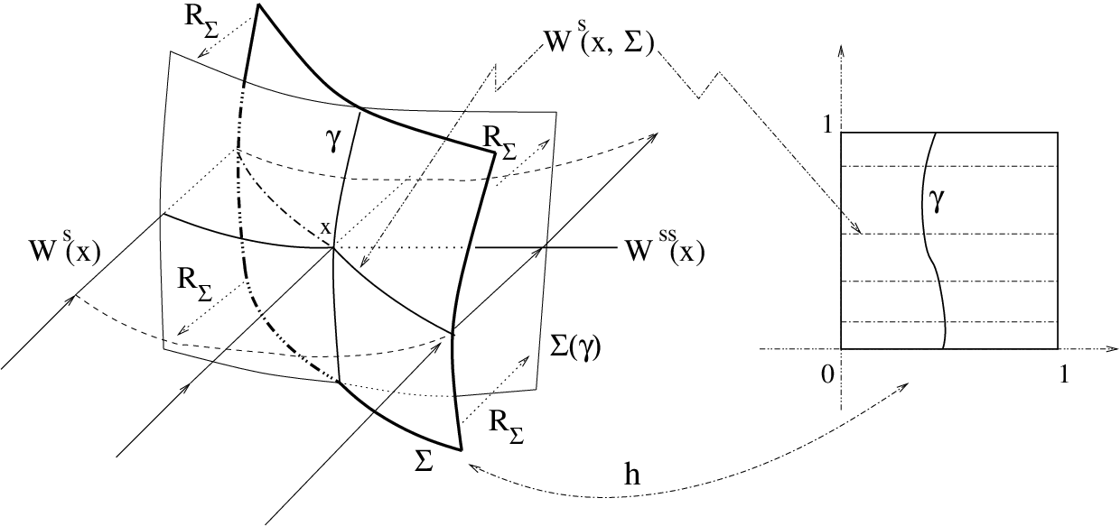
Given any cross-section $\Sigma$ and a point $x$ in its interior, we may always find a smaller cross-section also with $x$ in its interior and which is the image of the square $[0,1]\times[0,1]$ by a $C^{2}$ diffeomorphism $h$ that sends horizontal lines inside leaves of $\mathcal{F}^{s}_{\Sigma}$ . So, in what follows we always assume cross-sections are of the latter kind, see Figure 1. We denote by $\operatorname{int}(\Sigma)$ the image of $(0,1)\times(0,1)$ under the above-mentioned diffeomorphism, which we call the interior of $\Sigma$ .

We also assume that each cross-section $\Sigma$ is contained in $U_{0}$ , so that every $x\in\Sigma$ is such that $\omega(x)\subset\Lambda$ .

Remark 2.3.

In general, we can not choose the cross-section such that $W^{s}(x,\Sigma)\subset W^{ss}_{\varepsilon}(x)$ . The reason is that we want cross-sections to be $C^{2}$ . Cross-section of class $C^{1}$ are enough for the proof of expansiveness in Section 3 but $C^{2}$ is needed for the construction of the physical measure in Sections 5 through 5 and for the absolute continuity results in Section 8. The technical reason for this is explained in Section 5.2.

On the one hand $x\mapsto W^{ss}_{\varepsilon}(x)$ is usually not differentiable if we assume that $X$ is only of class $C^{1}$ . On the other hand, assuming that the cross-section is small with respect to $\varepsilon$ , and choosing any curve $\gamma\subset\Sigma$ crossing transversely every leaf of $\mathcal{F}_{\Sigma}^{s}$ , we may consider a Poincaré map

R_{\Sigma}:\Sigma\to\Sigma(\gamma)=\bigcup_{z\in\gamma}W^{ss}_{\varepsilon}(z)

with Poincaré time close to zero, see Figure 1. This is a homeomorphism onto its image, close to the identity, such that $R_{\Sigma}(W^{s}(x,\Sigma))\subset W^{ss}_{\varepsilon}(R_{\Sigma}(x))$ . So, identifying the points of $\Sigma$ with their images under this homeomorphism, we may pretend that indeed $W^{s}(x,\Sigma)\subset W^{ss}_{\varepsilon}(x)$ . We shall often do this in the sequel, to avoid cumbersome technicalities.

Refer to caption — Figure 1. The sections $\Sigma$ , $\Sigma(\gamma)$ , the manifolds $W^{s}(x),W^{ss}(x)$ , $W^{s}(x,\Sigma)$ and the projection $R_{\Sigma}$ , on the right. On the left, the square $[0,1]\times[0,1]$ is identified with $\Sigma$ through the map $h$ , where $\mathcal{F}_{\Sigma}^{s}$ becomes the horizontal foliation and the curve $\gamma$ is transversal to the horizontal direction. Solid lines with arrows indicate the flow direction.

2.2. Hyperbolicity of Poincaré maps

Let $\Sigma$ be a small cross-section to $X$ and let $R:\Sigma\to\Sigma^{\prime}$ be a Poincaré map $R(y)=X_{t(y)}(y)$ to another cross-section $\Sigma^{\prime}$ (possibly $\Sigma=\Sigma^{\prime}$ ). Note that $R$ needs not correspond to the first time the orbits of $\Sigma$ encounter $\Sigma^{\prime}$ , nor it is defined everywhere in $\Sigma$ .

The splitting $E^{s}\oplus E^{cu}$ over $U_{0}$ induces a continuous splitting $E_{\Sigma}^{s}\oplus E_{\Sigma}^{cu}$ of the tangent bundle $T\Sigma$ to $\Sigma$ (and analogously for $\Sigma^{\prime}$ ), defined by (recall (3) for the use of $E^{cs}$ )

(4)

E_{\Sigma}^{s}(y)=E^{cs}_{y}\cap T_{y}{\Sigma}\quad\mbox{and}\quad E_{\Sigma}^{cu}(y)=E^{cu}_{y}\cap T_{y}{\Sigma}.

We are going to prove that if the Poincaré time $t(x)$ is sufficiently large then (4) defines a hyperbolic splitting for the transformation $R$ on the cross-sections, at least restricted to $\Lambda$ :

Proposition 2.4.

Let $R:\Sigma\to\Sigma^{\prime}$ be a Poincaré map as before with Poincaré time $t(\cdot)$ . Then $DR_{x}(E_{\Sigma}^{s}(x))=E_{\Sigma}^{s}(R(x))$ at every $x\in\Sigma$ and $DR_{x}(E_{\Sigma}^{cu}(x))=E_{\Sigma}^{cu}(R(x))$ at every $x\in\Lambda\cap\Sigma$ .

Moreover for every given $0<\lambda<1$ there exists $t_{1}=t_{1}(\Sigma,\Sigma^{\prime},\lambda)>0$ such that if $t(\cdot)>t_{1}$ at every point, then

\|DR\mid E^{s}_{\Sigma}(x)\|<\lambda\quad\text{and}\quad\|DR\mid E^{cu}_{\Sigma}(x)\|>1/\lambda\quad\text{at every $x\in\Sigma$.}

Remark 2.5.

In what follows we use $K$ as a generic notation for large constants depending only on a lower bound for the angles between the cross-sections and the flow direction, and on upper and lower bounds for the norm of the vector field on the cross-sections. The conditions on $t_{1}$ in the proof of the proposition depend only on these bounds as well. In all our applications, all these angles and norms will be uniformly bounded from zero and infinity, and so both $K$ and $t_{1}$ may be chosen uniformly.

Proof.

The differential of the Poincaré map at any point $x\in\Sigma$ is given by

DR(x)=P_{R(x)}\circ DX_{t(x)}\mid T_{x}\Sigma,

where $P_{R(x)}$ is the projection onto $T_{R(x)}\Sigma^{\prime}$ along the direction of $X(R(x))$ . Note that $E^{s}_{\Sigma}(x)$ is tangent to $\Sigma\cap W^{s}(x)\supset W^{s}(x,\Sigma)$ . Since the stable manifold $W^{s}(x)$ is invariant, we have invariance of the stable bundle: $DR(x)\big(E^{s}_{\Sigma}(x)\big)=E^{s}_{\Sigma^{\prime}}\big(R(x)\big)$ . Moreover for all $x\in\Lambda$ we have

DX_{t(x)}\big(E^{cu}_{\Sigma}(x)\big)\subset DX_{t(x)}\big(E_{x}^{cu}\big)=E^{cu}_{R(x)}\,.

Since $P_{R(x)}$ is the projection along the vector field, it sends $E^{cu}_{R(x)}$ to $E^{cu}_{\Sigma^{\prime}}(R(x))$ . This proves that the center-unstable bundle is invariant restricted to $\Lambda$ , i.e. $DR(x)\big(E^{cu}_{\Sigma}(x)\big)=E^{cu}_{\Sigma^{\prime}}(R(x))$ .

Next we prove the expansion and contraction statements. We start by noting that $\|P_{R(x)}\|\leq K$ . Then we consider the basis $\{\frac{X(x)}{\|X(x)\|},\,e^{u}_{x}\}$ of $E^{cu}_{x}$ , where $e^{u}_{x}$ is a unit vector in the direction of $E^{cu}_{\Sigma}(x)$ . Since the flow direction is invariant, the matrix of $DX_{t}\mid E^{cu}_{x}$ relative to this basis is upper triangular:

DX_{t(x)}\mid E^{cu}_{x}=\left[\begin{array}[]{cc}\frac{\|X(R(x))\|}{\|X(x)\|}&\star\\ 0&\Delta\end{array}\right].

Moreover

\frac{1}{K}\cdot\operatorname{det}\big(DX_{t(x)}\mid E^{cu}_{x}\big)\leq\frac{\|X(R(x))\|}{\|X(x)\|}\Delta\leq K\cdot\operatorname{det}\big(DX_{t(x)}\mid E^{cu}_{x}\big).

Then

	$\displaystyle\\|DR(x)\,e^{u}_{x}\\|$	$\displaystyle=\\|P_{R(x)}\big(DX_{t(x)}(x)\cdot e^{u}_{x}\big)\\|=\\|\Delta\cdot e^{u}_{R(x)}\\|=\|\Delta\|$
		$\displaystyle\geq K^{-3}\,\|\operatorname{det}(DX_{t(x)}\mid E^{cu}_{x})\|\geq K^{-3}\lambda^{-t(x)}\geq K^{-3}\,\lambda^{-t_{1}}.$

Taking $t_{1}$ large enough we ensure that the latter expression is larger than $1/\lambda$ .

To prove $\|DR\mid E^{s}_{\Sigma}(x)\|<\lambda$ , let us consider unit vectors $e^{s}_{x}\in E^{s}_{x}$ and $\hat{e}^{s}_{x}\in E^{s}_{\Sigma}(x)$ , and write

e^{s}_{x}=a_{x}\cdot\hat{e}^{s}_{x}+b_{x}\cdot\frac{X(x)}{\|X(x)\|}\,.

Since $\sphericalangle(E^{s}_{x},X(x))\geq\sphericalangle(E_{x}^{s},E^{cu}_{x})$ and the latter is uniformly bounded from zero, we have $|a_{x}|\geq\kappa$ for some $\kappa>0$ which depends only on the flow. Then

(5)	$\displaystyle\\|DR(x)\,e_{x}^{s}\\|$	$\displaystyle=\\|P_{R(x)}\circ\big(DX_{t(x)}(x)\cdot e^{s}_{x}\big)\\|$
		$\displaystyle=\frac{1}{\|a_{x}\|}\,\left\\|P_{R(x)}\circ\Big(DX_{t(x)}(x)\big(e^{s}_{x}-b_{x}\frac{X(x)}{\\|X(x)\\|}\big)\Big)\right\\|$
		$\displaystyle=\frac{1}{\|a_{x}\|}\,\left\\|P_{R(x)}\circ\big(DX_{t(x)}(x)\cdot\hat{e}^{s}_{x}\big)\right\\|\leq\frac{K}{\kappa}\lambda^{t(x)}\leq\frac{K}{\kappa}\lambda^{t_{1}}.$

Once more it suffices to take $t_{1}$ large to ensure that the right hand side is less than $\lambda$ . ∎

Given a cross-section $\Sigma$ , a positive number $\rho$ , and a point $x\in\Sigma$ , we define the unstable cone of width $\rho$ at $x$ by

(6)

C_{\rho}^{u}(x)=\{v=v^{s}+v^{u}:v^{s}\in E^{s}_{\Sigma}(x),\,v^{u}\in E^{cu}_{\Sigma}(x)\mbox{ and }\|v^{s}\|\leq\rho\|v^{u}\|\}

(we omit the dependence on the cross-section in our notations).

Let $\rho>0$ be any small constant. In the following consequence of Proposition 2.4 we assume the neighborhood $U_{0}$ has been chose sufficiently small, depending on $\rho$ and on a bound on the angles between the flow and the cross-sections.

Corollary 2.6.

For any $R:\Sigma\to\Sigma^{\prime}$ as in Proposition 2.4, with $t(\cdot)>t_{1}$ , and any $x\in\Sigma$ , we have

DR(x)(C^{u}_{\rho}(x))\subset C_{\rho/2}^{u}(R(x))\quad\mbox{and}\quad\|DR_{x}(v)\|\geq\frac{5}{6}\lambda^{-1}\cdot\|v\|\quad\mbox{for all}\quad v\in C^{u}_{\rho}(x).

Proof.

Proposition 2.4 immediately implies that $DR_{x}(C^{u}_{\rho}(x))$ is contained in the cone of width $\rho/4$ around $DR(x)\big(E^{cu}_{\Sigma}(x)\big)$ relative to the splitting

T_{R(x)}\Sigma^{\prime}=E^{s}_{\Sigma^{\prime}}(R(x))\oplus DR(x)\big(E^{cu}_{\Sigma}(x)\big).

(We recall that $E^{s}_{\Sigma}$ is always mapped to $E^{s}_{\Sigma^{\prime}}$ .) The same is true for $E^{cu}_{\Sigma}$ and $E^{cu}_{\Sigma^{\prime}}$ , restricted to $\Lambda$ . So the previous observation already gives the conclusion of the first part of the corollary in the special case of points in the attractor. Moreover to prove the general case we only have to show that $DR(x)\big(E^{cu}_{\Sigma}(x)\big)$ belongs to a cone of width less than $\rho/4$ around $E^{cu}_{\Sigma^{\prime}}(R(x))$ . This is easily done with the aid of the flow invariant cone field $C_{a}^{cu}$ in (2), as follows. On the one hand,

DX_{t(x)}\big(E^{cu}_{\Sigma}(x)\big)\subset DX_{t(x)}\big(E^{cu}_{x}\big)\subset DX_{t(x)}\big(C^{cu}_{a}(x)\big)\subset C^{cu}_{a}(R(x))\,.

We note that $DR(x)\big(E^{cu}_{\Sigma}(x)\big)=P_{R(x)}\circ DX_{t(x)}\big(E^{cu}_{\Sigma}(x)\big)$ . Since $P_{R(x)}$ maps $E^{cu}_{R(x)}$ to $E^{cu}_{\Sigma^{\prime}}(R(x))$ and the norms of both $P_{R(x)}$ and its inverse are bounded by some constant $K$ (see Remark 2.5), we conclude that $DR(x)\big(E^{cu}_{\Sigma}(x)\big)$ is contained in a cone of width $b$ around $E^{cu}_{\Sigma^{\prime}}(R(x))$ , where $b=b(a,K)$ can be made arbitrarily small by reducing $a$ . We keep $K$ bounded, by assuming the angles between the cross-sections and the flow are bounded from zero and then, reducing $U_{0}$ if necessary, we can make $a$ small so that $b<\rho/4$ . This concludes the proof since the expansion estimate is a trivial consequence of Proposition 2.4. ∎

By a curve we always mean the image of a compact interval $[a,b]$ by a $C^{1}$ map. We use $\ell(\gamma)$ to denote its length. By a cu-curve in $\Sigma$ we mean a curve contained in the cross-section $\Sigma$ and whose tangent direction $T_{z}\gamma\subset C^{u}_{\rho}(z)$ for all $z\in\gamma$ . The next lemma says that cu-curves linking the stable leaves of nearby points must be short.

Lemma 2.7.

Let us assume that $\rho$ has been fixed, sufficiently small. Then there exists a constant $\kappa$ such that, for any pair of points $x,y\in\Sigma$ , and any cu-curve $\gamma$ joining $x$ to some point of $W^{s}(y,\Sigma)$ , we have $\ell(\gamma)\leq\kappa\cdot d(x,y)$ .

Here $d$ is the intrinsic distance in the $C^{2}$ surface $\Sigma$ .

Proof.

We consider coordinates on $\Sigma$ for which $x$ corresponds to the origin, $E^{cu}_{\Sigma}(x)$ corresponds to the vertical axis, and $E^{s}_{\Sigma}(x)$ corresponds to the horizontal axis; through these coordinates we identify $\Sigma$ with a subset of its tangent space at $x$ , endowed with the Euclidean metric. In general this identification is not an isometry, but the distortion is uniformly bounded, and that is taken care of by the constants $C_{1}$ and $C_{2}$ in what follows.

The hypothesis that $\gamma$ is a cu-curve implies that it is contained in the cone of width $C_{1}\cdot\rho$ centered at $x$ . On the other hand, stable leaves are close to being horizontal. It follows (see Figure 2) that the length of $\gamma$ is bounded by $C_{2}\cdot d(x,y)$ . This proves the lemma with $\kappa=C_{2}$ . ∎

In what follows we take $t_{1}$ in Proposition 2.4 for $\lambda=1/3$ . From Section 5 onwards we will need to decrease $\lambda$ once taking a bigger $t_{1}$ .

2.3. Adapted cross-sections

The next step is to exhibit stable manifolds for Poincaré transformations $R:\Sigma\to\Sigma^{\prime}$ . The natural candidates are the intersections $W^{s}(x,\Sigma)=W^{s}_{\varepsilon}(x)\cap\Sigma$ we introduced previously. These intersections are tangent to the corresponding sub-bundle $E^{s}_{\Sigma}$ and so, by Proposition 2.4, they are contracted by the transformation. For our purposes it is also important that the stable foliation be invariant:

(7)

R(W^{s}(x,\Sigma))\subset W^{s}(R(x),\Sigma^{\prime})\qquad\text{for every }x\in\Lambda\cap\Sigma.

In order to have this we restrict somewhat our class of cross-sections whose center-unstable boundary is disjoint from $\Lambda$ . Recall (Remark 2.2) that we are considering cross-sections $\Sigma$ that are diffeomorphic to the square $[0,1]\times[0,1]$ , with the horizontal lines $[0,1]\times\{\eta\}$ being mapped to stable sets $W^{s}(y,\Sigma)$ . The stable boundary $\partial^{s}\Sigma$ is the image of $[0,1]\times\{0,1\}$ . The center-unstable boundary $\partial^{cu}\Sigma$ is the image of $\{0,1\}\times[0,1]$ . The cross-section is $\delta$ -adapted if

d(\Lambda\cap\Sigma,\partial^{cu}\Sigma)>\delta,

where $d$ is the intrinsic distance in $\Sigma$ , see Figure 3. We call horizontal strip of $\Sigma$ the image $h([0,1]\times I)$ for any compact subinterval $I$ , where $h:[0,1]\times[0,1]\to\Sigma$ is the coordinate system on $\Sigma$ as in Remark 2.2. Notice that every horizontal strip is a $\delta$ -adapted cross-section.

In order to prove that adapted cross-sections do exist, we need the following result.

Lemma 2.8.

If $\Lambda$ is a singular-hyperbolic attractor, then every point $x\in\Lambda$ is in the closure of $W^{ss}(x)\setminus\Lambda$ .

Proof.

The proof is by contradiction. Let us suppose that there exists $x\in\Lambda$ such that $x$ is in the interior of $W^{ss}(x)\cap\Lambda$ . Let $\alpha(x)\subset\Lambda$ be its $\alpha$ -limit set. Then

(8)

W^{ss}(z)\subset\Lambda\quad\text{for every }z\in\alpha(x),

since any compact part of the strong-stable manifold of $z$ is accumulated by backward iterates of any small neighborhood of $x$ inside $W^{ss}(x)$ . It follows that $\alpha(x)$ does not contain any singularity: indeed, [37, Theorem B] proves that the strong-stable manifold of each singularity meets $\Lambda$ only at the singularity. Therefore by [37, Proposition 1.8] the invariant set $\alpha(x)\subset\Lambda$ is hyperbolic. It also follows from (8) that the union

S=\bigcup_{y\in\alpha(x)\cap\Lambda}W^{ss}(y)

of the strong-stable manifolds through the points of $\alpha(x)$ is contained in $\Lambda$ . By continuity of the strong-stable manifolds and the fact that $\alpha(x)$ is a closed set, we get that $S$ is also closed. Using [37] once more, we see that $S$ does not contain singularities and, thus, is also a hyperbolic set.

We claim that $W^{u}(S)$ , the union of the unstable manifolds of the points of $S$ , is an open set. To prove this, we note that $S$ contains the whole stable manifold $W^{s}(z)$ of every $z\in S$ : this is because $S$ is invariant and contains the strong-stable manifold of $z$ . Now, the union of the strong-unstable manifolds through the points of $W^{s}(z)$ contains a neighborhood of $z$ . This proves that $W^{u}(S)$ is a neighborhood of $S$ . Thus the backward orbit of any point in $W^{u}(S)$ must enter the interior of $W^{u}(S)$ . Since the interior is, clearly, an invariant set, this proves that $W^{u}(S)$ is open, as claimed.

Finally, consider any backward dense orbit in $\Lambda$ (we recall that for us an attractor is transitive by definition). On the one hand, its $\alpha$ -limit set is the whole $\Lambda$ . On the other hand, this orbit must intersect the open set $W^{u}(S)$ , and so the $\alpha$ -limit set must be contained in $S$ . This implies that $\Lambda\subset S$ , which is a contradiction, because $\Lambda$ contains singularities. ∎

Corollary 2.9.

For any $x\in\Lambda$ there exist points $x^{+}\notin\Lambda$ and $x^{-}\notin\Lambda$ in distinct connected components of $W^{ss}(x)\setminus\{x\}$ .

Proof.

Otherwise there would exist a whole segment of the strong-stable manifold entirely contained in $\Lambda$ . Considering any point in the interior of this segment, we would get a contradiction to Lemma 2.8. ∎

Lemma 2.10.

Let $x\in\Lambda$ be a regular point, that is, such that $X(x)\neq 0$ . Then there exists $\delta>0$ for which there exists a $\delta$ -adapted cross-section $\Sigma$ at $x$ .

Proof.

Fix $\varepsilon>0$ as in the stable manifold theorem. Any cross-section $\Sigma_{0}$ at $x$ sufficiently small with respect to $\varepsilon>0$ is foliated by the intersections $W_{\varepsilon}^{s}(x)\cap\Sigma_{0}$ . By Corollary 2.9, we may find points $x^{+}\notin\Lambda$ and $x^{-}\notin\Lambda$ in each of the connected components of $W^{s}_{\varepsilon}(x)\cap\Sigma_{0}$ . Since $\Lambda$ is closed, there are neighborhoods $V^{\pm}$ of $x^{\pm}$ disjoint from $\Lambda$ . Let $\gamma\subset\Sigma_{0}$ be some small curve through $x$ , transverse to $W^{s}_{\varepsilon}(x)\cap\Sigma_{0}$ . Then we may find a continuous family of segments inside $W^{s}_{\varepsilon}(y)\cap\Sigma_{0}$ , $y\in\gamma$ with endpoints contained in $V^{\pm}$ . The union $\Sigma$ of these segments is a $\delta$ -adapted cross-section, for some $\delta>0$ , see Figure 4.

∎

We are going to show that if the cross-sections are adapted, then we have the invariance property (7). Given $\Sigma,\Sigma^{\prime}\in\Xi$ we set $\Sigma(\Sigma^{\prime})=\{x\in\Sigma:R(x)\in\Sigma^{\prime}\}$ the domain of the return map from $\Sigma$ to $\Sigma^{\prime}$ .

Lemma 2.11.

Given $\delta>0$ and $\delta$ -adapted cross-sections $\Sigma$ and $\Sigma^{\prime}$ , there exists $t_{2}=t_{2}(\Sigma,\Sigma^{\prime})>0$ such that if $R:\Sigma(\Sigma^{\prime})\to\Sigma^{\prime}$ defined by $R(z)=R_{t(z)}(z)$ is a Poincaré map with time $t(\cdot)>t_{2}$ , then

(1)

$R\big(W^{s}(x,\Sigma)\big)\subset W^{s}(R(x),\Sigma^{\prime})$ for every $x\in\Sigma(\Sigma^{\prime})$ , and also
(2)

$d(R(y),R(z))\leq\frac{1}{2}\,d(y,z)$ for every $y$ , $z\in W^{s}(x,\Sigma)$ and $x\in\Sigma(\Sigma^{\prime})$ .

Proof.

This is a simple consequence of the relation (5) from the proof of Proposition 2.4: the tangent direction to each $W^{s}(x,\Sigma)$ is contracted at an exponential rate $\lambda$

\|DR(x)\,e_{x}^{s}\|\leq\frac{K}{\kappa}\lambda^{t(x)}.

Choosing $t_{2}$ sufficiently large we ensure that

\frac{1}{\kappa}\lambda^{t_{2}}\cdot\sup\{\ell(W^{s}(x,\Sigma)):x\in\Sigma\}<\delta.

In view of the definition of $\delta$ -adapted cross-section this gives part (1) of the lemma. Part (2) is entirely analogous: it suffices that $(K/\kappa)\cdot\lambda^{t_{2}}<1/2$ . ∎

Lemma 2.12.

Let $\Sigma$ be a $\delta$ -adapted cross-section. Then, given any $r>0$ there exists $\rho$ such that

d(y,z)<\rho\quad\Rightarrow\quad\operatorname{dist}(X_{s}(y),X_{s}(z))<r

for all $s>0$ , every $y$ , $z\in W^{s}(x,\Sigma)$ , and every $x\in\Lambda\cap\Sigma$ .

Remark 2.13.

Clearly we may choose $t_{2}>t_{1}$ . Remark 2.5 applies to $t_{2}$ as well.

Proof.

Let $y$ and $z$ be as in the statement. As in Remark 2.3, we may find $z^{\prime}=X_{\tau}(z)$ in the intersection of the orbit of $z$ with the strong-stable manifold of $y$ satisfying

\frac{1}{K}\leq\frac{\operatorname{dist}(y,z^{\prime})}{d(y,z)}\leq K\quad\text{and}\quad|\tau|\leq K\cdot d(y,z).

Then, given any $s>0$ ,

	$\displaystyle\operatorname{dist}(X_{s}(y),X_{s}(z))$	$\displaystyle\leq\operatorname{dist}(X_{s}(y),X_{s}(z^{\prime}))+\operatorname{dist}(X_{s}(z^{\prime}),X_{s}(z))$
		$\displaystyle\leq C\cdot e^{\gamma s}\cdot\operatorname{dist}(y,z^{\prime})+\operatorname{dist}(X_{s+\tau}(z),X_{s}(z))$
		$\displaystyle\leq KC\cdot e^{\gamma s}\cdot d(y,z)+K\|\tau\|\leq\big(KC+K^{2}\big)\cdot d(y,z).$

Taking $\rho<r/(KC+K^{2})$ we get the statement of the lemma. ∎

2.4. Flow boxes around singularities

In this section we collect some known facts about the dynamics near the singularities of the flow. It is known [36, Theorem A] that each singularity of a singular-hyperbolic attracting set, accumulated by regular orbits of a $3$ -dimensional flow, must be Lorenz-like. In particular every singularity $\sigma_{k}$ of a singular-hyperbolic attractor, as in the setting of Theorem A, is Lorenz-like, that is, the eigenvalues $\lambda_{1}\,,\lambda_{2}\,,\lambda_{3}$ of the derivative $DX(\sigma_{k})$ are all real and satisfy

\lambda_{1}>0>\lambda_{2}>\lambda_{3}\quad\text{and}\quad\lambda_{1}+\lambda_{2}>0.

In particular, the unstable manifold $W^{u}(\sigma_{k})$ is one-dimensional, and there is a one-dimensional strong-stable manifold $W^{ss}(\sigma_{k})$ contained in the two-dimensional stable manifold $W^{s}(\sigma_{k})$ . Most important for what follows, the attractor intersects the strong-stable manifold at the singularity only [36, Theorem A].

Then for some $\delta>0$ we may choose $\delta$ -adapted cross-sections contained in $U_{0}$

•

$\Sigma^{o,\pm}$ at points $y^{\pm}$ in different components of $W^{u}_{loc}(\sigma_{k})\setminus\{\sigma_{k}\}$
•

$\Sigma^{i,\pm}$ at points $x^{\pm}$ in different components of $W^{s}_{loc}(\sigma_{k})\setminus W^{ss}_{loc}(\sigma_{k})$

and Poincaré maps $R^{\pm}:\Sigma^{i,\pm}\setminus\ell^{\pm}\to\Sigma^{o,-}\cup\Sigma^{o,+}$ , where $\ell^{\pm}=\Sigma^{i,\pm}\cap W^{s}_{loc}(\sigma_{k}),$ satisfying (see Figure 5)

(1)

every orbit in the attractor passing through a small neighborhood of the singularity $\sigma_{k}$ intersects some of the incoming cross-sections $\Sigma^{i,\pm}$ ;
(2)

$R^{\pm}$ maps each connected component of $\Sigma^{i,\pm}\setminus\ell^{\pm}$ diffeomorphically inside a different outgoing cross-section $\Sigma^{o,\pm}$ , preserving the corresponding stable foliations and unstable cones.

These cross-sections may be chosen to be planar relative to some linearizing system of coordinates near $\sigma_{k}$ , e.g. for a small $\delta>0$

\Sigma^{i,\pm}=\{(x_{1},x_{2},\pm 1):|x_{1}|\leq\delta,|x_{2}|\leq\delta\}\quad\mbox{and}\quad\Sigma^{o,\pm}=\{(\pm 1,x_{2},x_{3}):|x_{2}|\leq\delta,|x_{3}|\leq\delta\},

where the $x_{1}$ -axis corresponds to the unstable manifold near $\sigma_{k}$ , the $x_{2}$ -axis to the strong-stable manifold and the $x_{3}$ -axis to the weak-stable manifold of the singularity which, in turn, is at the origin, see Figure 5.

Reducing the cross-sections if necessary, i.e. taking $\delta>0$ small enough, we ensure that the Poincaré times are larger than $t_{2}$ , so that the same conclusions as in the previous sections apply here. Indeed using linearizing coordinates it is easy to see that for points $z=(x_{1},x_{2},\pm 1)\in\Sigma^{i,\pm}$ the time $\tau^{\pm}$ it takes the flow starting at $z$ to reach one of $\Sigma^{o,\pm}$ depends on $x_{1}$ only and is given by

\tau^{\pm}(x_{1})=-\frac{\log x_{1}}{\lambda_{1}}.

We then fix these cross-sections once and for all and define for small $\varepsilon>0$ the flow-box

U_{\sigma_{k}}=\bigcup_{x\in\Sigma^{i,\pm}\setminus\ell^{\pm}}X_{(-\varepsilon,\tau^{\pm}(x)+\varepsilon)}(x)\cup(-\delta,\delta)\times(-\delta,\delta)\times(-1,1)

which is an open neighborhood of $\sigma_{k}$ with $\sigma_{k}$ the unique zero of $X\mid U_{\sigma_{k}}$ . We note that the function $\tau^{\pm}:\Sigma^{i,\pm}\to{\mathbb{R}}$ is integrable with respect to the Lebesgue (area) measure over $\Sigma^{i,\pm}$ : we say that the exit time function in a flow box near each singularity is Lebesgue integrable.

In particular we can determine the expression of the Poincaré maps between ingoing and outgoing cross-sections easily thought linearized coordinates

(9)

\Sigma^{i,+}\cap\{x_{1}>0\}\to\Sigma^{0,+},\quad(x_{1},x_{2},1)\mapsto\big(1,x_{2}\cdot x_{1}^{-\lambda_{3}/\lambda_{1}},x_{1}^{-\lambda_{2}/\lambda_{1}}\big).

This shows that the map obtained identifying points with the same $x_{2}$ coordinate, i.e. points in the same stable leaf, is simply $x_{1}\mapsto x_{1}^{\beta}$ where $\beta=-\lambda_{2}/\lambda_{1}\in(0,1)$ . For the other possible combinations of ingoing and outgoing cross-sections the Poincaré maps have a similar expression. This will be useful to construct physical measures for the flow.

3. Proof of expansiveness

Here we prove Theorem A. The proof is by contradiction: let us suppose that there exist $\varepsilon>0$ , a sequence $\delta_{n}\to 0$ , a sequence of functions $h_{n}\in S({\mathbb{R}})$ , and sequences of points $x_{n},\,y_{n}\in\Lambda$ such that

(10)

d\big(X_{t}(x_{n}),X_{h_{n}(t)}(y_{n})\big)\leq\delta_{n}\quad\text{for all }t\in{\mathbb{R}},

but

(11)

X_{h_{n}(t)}(y_{n})\notin X_{[t-\varepsilon,t+\varepsilon]}(x_{n})\quad\text{for all }t\in{\mathbb{R}}.

3.1. Proof of Theorem A

The main step in the proof is a reduction to a forward expansiveness statement about Poincaré maps which we state in Theorem 3.1 below.

We are going to use the following observation: there exists some regular (i.e. non-equilibrium) point $z\in\Lambda$ which is accumulated by the sequence of $\omega$ -limit sets $\omega(x_{n})$ . To see that this is so, start by observing that accumulation points do exist, since the ambient space is compact. Moreover, if the $\omega$ -limit sets accumulate on a singularity then they also accumulate on at least one of the corresponding unstable branches which, of course, consists of regular points. We fix such a $z$ once and for all. Replacing our sequences by subsequences, if necessary, we may suppose that for every $n$ there exists $z_{n}\in\omega(x_{n})$ such that $z_{n}\to z$ .

Let $\Sigma$ be a $\delta$ -adapted cross-section at $z$ , for some small $\delta$ . Reducing $\delta$ (but keeping the same cross-section) we may ensure that $z$ is in the interior of the subset

\Sigma_{\delta}=\{y\in\Sigma:d(y,\partial\Sigma)>\delta\}.

By definition the orbit of $x_{n}$ returns infinitely often to a neighborhood of $z_{n}$ which, on its turn, is close to $z$ . Thus dropping a finite number of terms in our sequences if necessary, we have that the orbit of $x_{n}$ intersects $\Sigma$ infinitely many times. Let $t_{n}$ be the time corresponding to the first intersection. Replacing $x_{n}$ , $y_{n}$ , $t$ , and $h_{n}$ by $x^{(n)}=X_{t_{n}}(x_{n})$ , $y^{(n)}=X_{h_{n}(t_{n})}(y_{n})$ , $t^{\prime}=t-t_{n}$ , and $h_{n}^{\prime}(t^{\prime})=h_{n}(t^{\prime}+t_{n})-h_{n}(t_{n})$ , we may suppose that $x^{(n)}\in\Sigma_{\delta}$ , while preserving both relations (10) and (11). Moreover there exists a sequence $\tau_{n,j}$ , $j\geq 0$ with $\tau_{n,0}=0$ such that

(12)

x^{(n)}(j)=X_{\tau_{n,j}}(x^{(n)})\in\Sigma_{\delta}\quad\text{and}\quad\tau_{n,j}-\tau_{n,j-1}>\max\{t_{1},t_{2}\}

for all $j\geq 1$ , where $t_{1}$ is given by Proposition 2.4 and $t_{2}$ is given by Lemma 2.11.

Theorem 3.1.

Given $\varepsilon_{0}>0$ there exists $\delta_{0}>0$ such that if $x\in\Sigma_{\delta}$ and $y\in\Lambda$ satisfy

(a)

there exist $\tau_{j}$ such that

$x_{j}=X_{\tau_{j}}(x)\in\Sigma_{\delta}\quad\text{and}\quad\tau_{j}-\tau_{j-1}>\max\{t_{1},t_{2}\}\quad\text{for all $j\geq 1$};$
(b)

$\operatorname{dist}\big(X_{t}(x),X_{h(t)}(y)\big)<\delta_{0}$ , for all $t>0$ and some $h\in S({\mathbb{R}})$ ;

then there exists $s\in{\mathbb{R}}$ such that $X_{h(s)}(y)\in W_{\varepsilon_{0}}^{ss}(X_{[s-\varepsilon_{0},s+\varepsilon_{0}]}(x))$ .

We postpone the proof of Theorem 3.1 until the next section and explain first why it implies Theorem A. We are going to use the following observation.

Lemma 3.2.

There exist $\rho>0$ small and $c>0$ , depending only on the flow, such that if $z_{1},z_{2},z_{3}$ are points in $\Lambda$ satisfying $z_{3}\in X^{[-\rho,\rho]}(z_{2})$ and $z_{2}\in W_{\rho}^{ss}(z_{1})$ , then

\operatorname{dist}(z_{1},z_{3})\geq c\cdot\max\{\operatorname{dist}(z_{1},z_{2}),\operatorname{dist}(z_{2},z_{3})\}.

Proof.

This is a direct consequence of the fact that the angle between $E^{ss}$ and the flow direction is bounded from zero which, on its turn, follows from the fact that the latter is contained in the center-unstable sub-bundle $E^{cu}$ . Indeed consider for small enough $\rho>0$ the $C^{1}$ surface $X^{[-\rho,\rho]}\big(W^{ss}_{\rho}(z_{1})\big)$ . The Riemannian metric here is uniformly close to the Euclidean one and we may choose coordinates on $[-\rho,\rho]^{2}$ putting $z_{1}$ at the origin, sending $W^{ss}_{\rho}(z_{1})$ to the segment $[-\rho,\rho]\times\{0\}$ and $X^{[-\rho,\rho]}(z_{1})$ to $\{0\}\times[-\rho,\rho]$ , see Figure 6.

Then the angle $\alpha$ between $X^{[-\rho,\rho]}(z_{2})$ and the horizontal is bounded from below away from zero and the existence of $c$ follows by standard arguments using the Euclidean metric. ∎

We fix $\varepsilon_{0}=\varepsilon$ as in (11) and then consider $\delta_{0}$ as given by Theorem 3.1. Next, we fix $n$ such that $\delta_{n}<\delta_{0}$ and $\delta_{n}<c\rho$ , and apply Theorem 3.1 to $x=x^{(n)}$ and $y=y^{(n)}$ and $h=h_{n}$ . Hypothesis (a) in the theorem corresponds to (12) and, with these choices, hypothesis (b) follows from (10). Therefore we obtain that $X_{h(s)}(y)\in W_{\varepsilon}^{ss}(X_{[s-\varepsilon,s+\varepsilon]}(x))$ . In other words, there exists $|\tau|\leq\varepsilon$ such that $X_{h(s)}(y)\in W_{\varepsilon}^{ss}(X_{s+\tau}(x))$ . Hypothesis (11) implies that $X_{h(s)}(y)\neq X_{s+\tau}(x)$ . Since strong-stable manifolds are expanded under backward iteration, there exists $\theta>0$ maximum such that

X_{h(s)-t}(y)\in W^{ss}_{\rho}(X_{s+\tau-t}(x))\quad\text{and}\quad X_{h(s+\tau-t)}(y)\in X_{[-\rho,\rho]}(X_{h(s)-t}(y))

for all $0\leq t\leq\theta$ , see Figure 7. Since $\theta$ is maximum

\displaystyle\text{either }\operatorname{dist}\big(X_{h(s)-t}(y),X_{s+\tau-t}(x)\big)=\rho,\,\text{ or }\operatorname{dist}\big(X_{h(s+\tau-t)}(y),X_{h(s)-t}(y)\big)=\rho\text{ for }t=\theta.

Using Lemma 3.2, we conclude that

\operatorname{dist}(X_{s+\tau-t}(x),X_{h(s+\tau-t)}(y))\geq c\rho>\delta_{n}

which contradicts (10). This contradiction reduces the proof of Theorem A to that of Theorem 3.1.

3.2. Infinitely many coupled returns

We start by outlining the proof of Theorem 3.1. There are three steps.

•

The first one, which we carry out in the present section, is to show that to each return $x_{j}$ of the orbit of $x$ to $\Sigma$ there corresponds a nearby return $y_{j}$ of the orbit of $y$ to $\Sigma$ . The precise statement is in Lemma 3.3 below.
•

The second, and most crucial step, is to show that there exists a smooth Poincaré map, with large return time, defined on the whole strip of $\Sigma$ in between the stable manifolds of $x_{j}$ and $y_{j}$ . This is done in Section 3.3.
•

The last step, Section 3.3.4, is to show that these Poincaré maps are uniformly hyperbolic, in particular, they expand $cu$ -curves uniformly (recall the definition of $cu$ -curve in Section 2.2).

The theorem is then easily deduced: to prove that $X_{h(s)}(y)$ is in the orbit of $W_{\varepsilon}^{ss}(x)$ it suffices to show that $y_{j}\in W^{s}(x_{j},\Sigma)$ , by Remark 2.3. The latter must be true, for otherwise, by hyperbolicity of the Poincaré maps, the stable manifolds of $x_{j}$ and $y_{j}$ would move apart as $j\to\infty$ , and this would contradict condition (b) of Theorem 3.1. See Section 3.3.4 for more details.

Lemma 3.3.

There exists $K>0$ such that, in the setting of Theorem 3.1, there exists a sequence $(\upsilon_{j})_{j\geq 0}$ such that

(1)

$y_{j}=X_{\upsilon_{j}}(y)$ is in $\Sigma$ for all $j\geq 0$ ;
(2)

$|\upsilon_{j}-h(\tau_{j})|<K\cdot\delta_{0}$ , and
(3)

$d(x_{j},y_{j})<K\cdot\delta_{0}$ .

Proof.

By assumption $d(x_{j},X_{h(\tau_{j})}(y))<K\cdot\delta_{0}$ for all $j\geq 0$ . In particular $y^{\prime}_{j}=X_{h(\tau_{j})}(y)$ is close to $\Sigma$ . Using a flow box in a neighborhood of $\Sigma$ we obtain $X_{\varepsilon_{j}}(y_{j}^{\prime})\in\Sigma$ for some $\varepsilon_{j}\in(-K\cdot\delta_{0},K\cdot\delta_{0})$ . The constant $K$ depends only on the vector field $X$ and the cross-section $\Sigma$ (more precisely, on the angle between $\Sigma$ and the flow direction). Taking $\upsilon_{j}=h(\tau_{j})+\varepsilon_{j}$ we get the first two claims in the lemma. The third one follows from the triangle inequality; it may be necessary to replace $K$ by a larger constant, still depending on $X$ and $\Sigma$ only. ∎

3.3. Semi-global Poincaré map

Since we took the cross-section $\Sigma$ to be adapted, we may use Lemma 2.11 to conclude that there exist Poincaré maps $R_{j}$ with $R_{j}(x_{j})=x_{j+1}$ and $R_{j}(y_{j})=y_{j+1}$ and sending $W^{s}_{\varepsilon}(x_{j}\,,\Sigma)$ and $W^{s}_{\varepsilon}(y_{j}\,,\Sigma)$ inside $W^{s}_{\varepsilon}(x_{j+1}\,,\Sigma)$ and $W^{s}_{\varepsilon}(y_{j+1}\,,\Sigma)$ , respectively. The goal of this section is to prove that $R_{j}$ extends to a smooth Poincaré map on the whole strip $\Sigma_{j}$ of $\Sigma$ bounded by the stable manifolds of $x_{j}$ and $y_{j}$ .

We first outline the proof. For each $j$ we choose a curve $\gamma_{j}$ transverse to the stable foliation of $\Sigma$ , connecting $x_{j}$ to $y_{j}$ and such that $\gamma_{j}$ is disjoint from the orbit segments $[x_{j}\,,x_{j+1}]$ and $[y_{j}\,,y_{j+1}]$ . Using Lemma 2.11 in the same way as in the last paragraph, we see that it suffices to prove that $R_{j}$ extends smoothly to $\gamma_{j}$ . For this purpose we consider a tube-like domain $\mathcal{T}_{j}$ consisting of local stable manifolds through an immersed surface $S_{j}$ whose boundary is formed by $\gamma_{j}$ and $\gamma_{j+1}$ and the orbit segments $[x_{j}\,,x_{j+1}]$ and $[y_{j}\,,y_{j+1}]$ , see Figure 8. We will prove that the orbit of any point in $\gamma_{j}$ must leave the tube through $\gamma_{j+1}$ in finite time.

We begin by showing that the tube contains no singularities. This uses hypothesis (b) together with the local dynamics near Lorenz-like singularities. Next, using hypothesis (b) together with a Poincaré-Bendixson argument on $S_{j}$ , we conclude that the forward orbit of any point in $\mathcal{T}_{j}$ must leave the tube. Another argument, using hyperbolicity properties of the Poincaré map, shows that orbits through $\gamma_{j}$ must leave $\mathcal{T}_{j}$ through $\gamma_{j+1}$ . In the sequel we detail these arguments.

3.3.1. A tube-like domain without singularities

Since we took $\gamma_{j}$ and $\gamma_{j+1}$ disjoint from the orbit segments $[x_{j}\,,x_{j+1}]$ and $[y_{j}\,,y_{j+1}]$ , the union of these four curves is an embedded circle. We recall that the two orbit segments are close to each other, by hypothesis (b)

d(X_{t}(x),X_{h(t)}(y))<\delta_{0}\quad\text{for all $t\in[t_{j},t_{j+1}]$.}

Assuming that $\delta_{0}$ is smaller than the radius of injectiveness of the exponential map of the ambient manifold (i.e. $\exp_{x}:T_{x}M\to M$ is locally invertible in a $\delta_{0}$ -neighborhood of $x$ in $M$ for any $x\in M$ ), there exists a unique geodesic linking each $X_{t}(x)$ to $X_{h(t)}(y)$ , and it varies continuously (even smoothly) with $t$ . Using these geodesics we easily see that the union of $[y_{j}\,,y_{j+1}]$ with $\gamma_{j}$ and $\gamma_{j+1}$ is homotopic to a curve inside the orbit of $x$ , with endpoints $x_{j}$ and $x_{j+1}$ , and so it is also homotopic to the segment $[x_{j},x_{j+1}]$ . This means that the previously mentioned embedded circle is homotopic to zero. It follows that there is a smooth immersion $\phi:[0,1]\times[0,1]\to M$ such that

•

$\phi(\{0\}\times[0,1])=\gamma_{j}$ and $\phi(\{1\}\times[0,1])=\gamma_{j+1}$ ;
•

$\phi([0,1]\times\{0\})=[y_{j}\,,y_{j+1}]$ and $\phi([0,1]\times\{1\})=[x_{j}\,,x_{j+1}]$ .

Moreover $S_{j}=\phi([0,1]\times[0,1])$ may be chosen such that

•

all the points of $S_{j}$ are at distance less than $\delta_{1}$ from the orbit segment $[x_{j}\,,x_{j+1}]$ , for some uniform constant $\delta_{1}>\delta_{0}$ which can be taken arbitrarily close to zero, reducing $\delta_{0}$ if necessary, see Figure 8;
•

the intersection of $S_{j}$ with an incoming cross-section of any singularity (Section 2.4) is transverse to the corresponding stable foliation, see Figure 9.

Then we define $\mathcal{T}_{j}$ to be the union of the local stable manifolds through the points of that disk.

Proposition 3.4.

The domain $\mathcal{T}_{j}$ contains no singularities of the flow.

Proof.

By construction, every point of $\mathcal{T}_{j}$ is at distance $\leq\varepsilon$ from $S_{j}$ and, consequently, at distance $\leq\varepsilon+\delta_{1}$ from $[x_{j}\,,x_{j+1}]$ . So, taking $\varepsilon$ and $\delta_{0}$ much smaller than the sizes of the cross-sections associated to the singularities (Section 2.4), we immediately get the conclusion of the proposition in the case when $[x_{j}\,,x_{j+1}]$ is disjoint from the incoming cross-sections of all singularities. In the general case we must analyze the intersections of the tube with the flow boxes at the singularities. The key observation is in the following statement whose proof we postpone.

Lemma 3.5.

Suppose $[x_{j}\,,x_{j+1}]$ intersects an incoming cross-section $\Sigma_{k}^{i}$ of some singularity $\sigma_{k}$ at some point $\hat{x}$ with $d(\hat{x},\partial\Sigma_{k}^{i})>\delta$ . Then $[y_{j}\,,y_{j+1}]$ intersects $\Sigma_{k}^{i}$ at some point $\hat{y}$ with $d(\hat{x},\hat{y})<K\cdot\delta_{0}$ and, moreover $\hat{x}$ and $\hat{y}$ are in the same connected component of $\Sigma_{k}^{i}\setminus W_{loc}^{s}(\sigma_{k})$ .

Let us recall that by construction the intersection of $S_{j}$ with the incoming cross-section $\Sigma_{k}^{i}$ is transverse to the corresponding stable foliation, see Figure 9. By the previous lemma this intersection is entirely contained in one of the connected components of $\Sigma_{k}^{i}\setminus W^{s}_{loc}(\sigma_{k})$ . Since $\mathcal{T}_{j}$ consists of local stable manifolds through the points of $S_{j}$ its intersection with $\Sigma_{k}^{i}$ is contained in the region bounded by the stable manifolds $W^{s}(\hat{x},\Sigma_{k}^{i})$ and $W^{s}(\hat{y},\Sigma_{k}^{i})$ , and so it is entirely contained in a connected component of $\Sigma_{k}^{i}\setminus W^{s}_{loc}(\sigma_{k})$ . In other words, the crossing of the tube $\mathcal{T}_{j}$ through the flow box is disjoint from $W^{s}_{loc}(\sigma_{k})$ , in particular, it does not contain the singularity. Repeating this argument for every intersection of the tube with a neighborhood of some singularity, we get the conclusion of the proposition. ∎

Proof of Lemma 3.5.

The first part is proved in exactly the same way as Lemma 3.3. We have

\hat{x}=X_{r_{0}}(x)\quad\text{and}\quad\hat{y}=X_{s_{0}}(y)

with $|s_{0}-h(r_{0})|<K\delta_{0}$ . The proof of the second part is by contradiction and relies, fundamentally, on the local description of the dynamics near the singularity. Associated to $\hat{x}$ and $\hat{y}$ we have the points $\tilde{x}=X_{r_{1}}(x)$ and $\tilde{y}=X_{s_{1}}(y)$ , where the two orbits leave the flow box associated to the singularity. If $\hat{x}$ and $\hat{y}$ are in opposite sides of the local stable manifold of $\sigma_{k}$ , then $\tilde{x}$ and $\tilde{y}$ belong to different outgoing cross-sections of $\sigma_{k}$ . Our goal is to find some $t\in{\mathbb{R}}$ such that

\operatorname{dist}\big(X_{t}(x),X_{h(t)}(y)\big)>\delta_{0}\,,

thus contradicting hypothesis (b).

We assume by contradiction that $\hat{x},\hat{y}$ are in different connected components of $\Sigma_{k}^{i,\pm}\setminus\ell^{\pm}$ . There are two cases to consider. We suppose first that $h(r_{1})>s_{1}$ and note that $s_{1}\gg s_{0}\approx h(r_{0})$ , so that $s_{1}>h(r_{0})$ . It follows that there exists $t\in(r_{0},r_{1})$ such that $h(t)=s_{1}$ since $h$ is non-decreasing and continuous. Then $X_{t}(x)$ is on one side of the flow box of $\sigma_{k}$ , whereas $X_{h(t)}(y)$ belongs to the outgoing cross-section at the other side of the flow box. Thus $\operatorname{dist}\big(X_{t}(x),X_{h(t)}(y)\big)$ has the order of magnitude of the diameter of the flow box, which we may assume to be much larger than $\delta_{0}$ .

Now we suppose that $s_{1}\geq h(r_{1})$ and observe that $h(r_{1})>h(r_{0})$ , since $h$ is increasing. We recall also that $X_{h(r_{0})}(y)$ is close to $\hat{y}$ , near the incoming cross-section, so that the whole orbit segment from $X_{h(r_{0})}(y)$ to $X_{s_{1}}(y)$ is contained in (a small neighborhood of) the flow box, to one side of the local stable manifold of $\sigma_{j}$ . The previous observation means that this orbit segment contains $X_{h(r_{1})}(y)$ . However $X_{r_{1}}(x)$ belongs to the outgoing cross-section at the opposite side of the flow box, and so $\operatorname{dist}\big(X_{r_{1}}(x),X_{h(r_{1})}(y)\big)$ has the order of magnitude of the diameter of the flow box, which is much larger than $\delta_{0}$ . ∎

3.3.2. Every orbit leaves the tube

Our goal in this section is to show that the forward orbit of every point $z\in\mathcal{T}_{j}$ leaves the tube in finite time. The proof is based on a Poincaré-Bendixson argument applied to the flow induced by $X^{t}$ on the immersed disk $S_{j}$ .

We begin by defining this induced flow. For the time being, we make the following simplifying assumption:

(H)

$S_{j}=\phi([0,1]\times[0,1])$ is an embedded disk and the stable manifolds $W^{s}_{\varepsilon}(\xi)$ through the points $\xi\in S_{j}$ are pairwise disjoint.

This condition provides a well-defined continuous projection $\pi:\mathcal{T}_{j}\to S_{j}$ by assigning to each point $z\in\mathcal{T}_{j}$ the unique $\xi\in S_{j}$ whose local strong-stable manifold contains $z$ . The (not necessarily complete) flow $Y_{t}$ induced by $X_{t}$ on $S_{j}$ is given by $Y_{t}(\xi)=\pi(X_{t}(\xi))$ for the largest interval of values of $t$ for which this is defined. It is clear, just by continuity, that given any subset $E$ of $S_{j}$ at a positive distance from $\partial S_{j}$ , there exists $\varepsilon>0$ such that $Y_{t}(\xi)$ is defined for all $\xi\in E$ and $t\in[0,\varepsilon]$ . In fact this remains true even if $E$ approaches the curve $\gamma_{j}$ (since $\Sigma$ is a cross-section for $X_{t}$ , the flow at $\gamma_{j}$ points inward $S_{j}$ ) or the $X_{t}$ -orbit segments $[x_{j}\,,x_{j+1}]$ and $[y_{j}\,,y_{j+1}]$ on the boundary of $S_{j}$ (because they are also $Y_{t}$ -orbit segments). Thus we only have to worry with the distance to the remaining boundary segment:

(U)

given any subset $E$ of $S_{j}$ at positive distance from $\gamma_{j+1}$ , there exists $\varepsilon>0$ such that $Y_{t}(\xi)$ is defined for all $\xi\in E$ and $t\in[0,\varepsilon]$ .

We observe also that for points $\xi$ close to $\gamma_{j+1}$ the flow $Y_{t}(\xi)$ must intersect $\gamma_{j+1}$ , after which it is no longer defined.

Now we explain how to remove condition (H). In this case, the induced flow is naturally defined on $[0,1]\times[0,1]$ rather than $S_{j}$ , as we now explain. We recall that $\phi:[0,1]\times[0,1]\to M$ is an immersion. So given any $w\in[0,1]\times[0,1]$ there exist neighborhoods $U$ of $w$ and $V$ of $\phi(w)$ in $S_{j}$ such that $\phi:U\to V$ is a diffeomorphism. Moreover, just by continuity of the stable foliation, choosing $V$ sufficiently small we may ensure that each strong-stable manifold $W_{\varepsilon}^{ss}(\xi)$ , $\xi\in V$ , intersects $V$ only at the point $\xi$ . This means that we have a well-defined projection $\pi$ from $\cup_{\xi\in V}W_{\varepsilon}^{ss}(\xi)$ to $V$ associating to each point $z$ in the domain the unique element of $V$ whose stable manifold contains $z$ . Then we may define $Y_{t}(w)$ for small $t$ , by

Y_{t}(w)=\phi^{-1}(\pi(X_{t}(\phi(w))).

As before, we extend $Y_{t}$ to a maximal domain. This defines a (partial) flow on the square $[0,1]\times[0,1]$ , such that both $[0,1]\times\{i\}$ , $i\in\{0,1\}$ are trajectories.

Remark 3.6.

A singularity $\zeta$ for the flow $Y_{t}$ corresponds to a singularity of $X$ in the local strong-stable manifold of $\zeta$ in $M$ by the definition of $Y_{t}$ through the projection $\pi$ .

Notice also that forward trajectories of points in $\{0\}\times[0,1]$ enter the square. Hence, the only way trajectories may exit is through $\{1\}\times[0,1]$ . So, we have the following reformulation of property (U):

(U)

given any subset $E$ of $[0,1]\times[0,1]$ at positive distance from $\{1\}\times[0,1]$ , there exists $\varepsilon>0$ such that $Y_{t}(w)$ is defined for all $w\in E$ and $t\in[0,\varepsilon]$ .

Moreover for points $w$ close to $\{1\}\times[0,1]$ the flow $Y_{t}(\xi)$ must intersect $\{1\}\times[0,1]$ , after which it is no longer defined.

Proposition 3.7.

Given any point $z\in\mathcal{T}_{j}$ there exists $t>0$ such that $X_{t}(z)\notin\mathcal{T}_{j}$ .

Proof.

The proof is by contradiction. First, we assume condition (H). Suppose there exists $z\in\mathcal{T}_{j}$ whose forward orbit remains in the tube for all times. Let $z_{0}=\pi(z)$ . Then $Y_{t}(z_{0})$ is defined for all $t>0$ , and so it makes sense to speak of the $\omega$ -limit set $\omega(z_{0})$ . The orbit $Y_{t}(z_{0})$ can not accumulate on $\gamma_{j+1}$ for otherwise it would leave $S_{j}$ . Therefore $\omega(z_{0})$ is a compact subset of $S_{j}$ at positive distance from $\gamma_{j+1}$ . Using property (U) we can find a uniform constant $\varepsilon>0$ such that $Y_{t}(w)$ is defined for every $t\in[0,\varepsilon]$ and every $w\in\omega(z_{0})$ . Since $\omega(z_{0})$ is an invariant set, we can extend $Y_{t}$ to a complete flow on it.

In particular we may fix $w_{0}\in\omega(z_{0})$ , $w\in\omega(w_{0})$ and apply the arguments in the proof of the Poincaré-Bendixson Theorem. On the one hand, if we consider a cross-section $S$ to the flow at $w$ , the forward orbits of $z_{0}$ and $w_{0}$ must intersect it on monotone sequences; on the other hand, every intersection of the orbit of $w_{0}$ with $S$ is accumulated by points in the orbit of $z_{0}$ . This implies that $w$ is in the orbit of $w_{0}$ and, in fact, that the later is periodic.

We consider the disk $D\subset S_{j}$ bounded by the orbit of $w_{0}$ . The flow $Y_{t}$ is complete restricted to $D$ and so we may apply Poincaré-Bendixson’s Theorem (see [39]) once more, and conclude that $Y_{t}$ has some singularity $\zeta$ inside $D$ . This implies by Remark 3.6 that $X_{t}$ has a singularity in the local stable manifold of $\zeta$ , which contradicts Proposition 3.4. This contradiction completes the proof of the proposition, under assumption (H). The general case is treated in the same way, just dealing with the flow induced on $[0,1]\times[0,1]$ instead of on $S_{j}$ . ∎

3.3.3. The Poincaré map is well-defined on $\Sigma_{j}$

We have shown that for the induced flow $Y_{t}$ on $S_{j}$ (or, more generally, on $[0,1]\times[0,1]$ ) every orbit must eventually cross $\gamma_{j+1}$ (respectively, $\{1\}\times[0,1]$ ). Hence there exists a continuous Poincaré map

r:\gamma_{j}\to\gamma_{j+1},\quad r(\xi)=Y_{\theta(\xi)}(\xi).

By compactness the Poincaré time $\theta(\cdot)$ is bounded. We are going to deduce that every forward $X_{t}$ -orbit eventually leaves the tube $\mathcal{T}_{j}$ through $\Sigma_{j+1}$ (the strip in $\Sigma$ between the stable manifolds $W^{s}(x_{j+1},\Sigma)$ and $W^{s}(y_{j+1},\Sigma)$ ), which proves that $R_{j}$ is defined on the whole strip of $\Sigma_{j}$ between the manifolds $W^{s}(x_{j},\Sigma_{j})$ and $W^{s}(y_{j},\Sigma_{j})$ , as claimed in Section 3.2.

To this end, let $\gamma$ be a central-unstable curve in $\Sigma_{\delta}$ connecting the stable manifolds $W^{s}(x_{j},\Sigma)$ and $W^{s}(y_{j},\Sigma)$ . Observe that $\gamma$ is inside $\mathcal{T}_{j}$ . For each $z\in\gamma$ , let $t(z)$ be the smallest positive time for which $X_{t(z)}$ is on the boundary of $\mathcal{T}_{j}$ .

The crucial observation is that, in view of the construction of $Y_{t}$ , each $X_{t(\xi)}(\xi)$ belongs to the stable manifold of $Y_{t(z)}\big(\pi(z)\big)$ . We observe also that for $\{\xi\}=\gamma\cap W^{s}(x_{j},\Sigma)$ we have $Y_{t}(\xi)=X_{t}(\xi)$ and so $t(\xi)=\theta(\xi)$ .

Now we take $z\in\gamma$ close to $\xi$ . Just by continuity the $X_{t}$ -trajectories of $\xi$ and $z$ remain close, and by the forward contraction along stable manifolds, the $X_{t}$ -trajectory of $\xi$ remains close to the segment $[x_{j},x_{j+1}]$ . Moreover the orbit of $z$ cannot leave the tube through the union of the local strong stable manifolds passing through $[x_{j},x_{j+1}]$ , for otherwise it would contradict the definition of $Y_{t}$ . Hence the trajectory of $z$ must leave the tube through $\Sigma_{j+1}$ . In other words $X_{t(z)}(z)$ is a point of $\Sigma_{j+1}$ , close to $X_{t(\xi)}(\xi)$ .

Let $\hat{\gamma}\subset\gamma$ be the largest connected subset containing $\xi$ such that $X_{t(z)}(z)\in\Sigma_{j+1}$ for all $z\in\hat{\gamma}$ . We want to prove that $\hat{\gamma}=\gamma$ since this implies that $R_{j}$ extends to the whole $\gamma_{j}$ and so, using Lemma 2.11, to the whole strip of $\Sigma_{j}$ .

The proof is by contradiction. We assume $\hat{\gamma}$ is not the whole $\gamma$ , and let $\hat{x}$ be the endpoint different from $\xi$ . Then by definition of $\mathcal{F}_{\Sigma}^{s}$ and of $Y_{t}$ (from Section 3.3.2) $\tilde{x}=X_{t(\hat{x})}(\hat{x})$ is on the center-unstable boundary $\partial^{cu}\Sigma_{j+1}$ of the cross-section $\Sigma_{j+1}$ , between the stable manifolds $W^{s}(x_{j+1},\Sigma_{j+1})$ and $W^{s}(y_{j+1},\Sigma_{j+1})$ , see Figure 10.

By the choice of $\gamma$ and by Corollary 2.6, $\tilde{\gamma}=\{X_{t(z)}(z):z\in\hat{\gamma}\}$ is a $cu$ -curve. On the one hand, by Lemma 2.7, the distance between $\tilde{x}$ and $\tilde{\xi}=X_{t(\xi)}(\xi)$ dominates the distance between their stable manifolds and $\ell(\tilde{\gamma})$

\ell(\tilde{\gamma})\leq\kappa\cdot d(\xi,\tilde{x})\leq\kappa\cdot d\big(W^{s}(x_{j+1},\Sigma),W^{s}(\tilde{x},\Sigma)\big).

We note that $\ell(\tilde{\gamma})$ is larger than $\delta$ , since $\xi$ is in $\Sigma_{\delta}$ and the section $\Sigma_{j+1}$ is adapted. On the other hand, the distance between the two stable manifolds is smaller than the distance between the stable manifold of $x_{j+1}$ and the stable manifold of $y_{j+1}$ , and this is smaller than $K\cdot\delta_{0}$ . Since $\delta_{0}$ is much smaller than $\delta$ , this is a contradiction. This proves the claim that $X_{t(z)}(z)\in\Sigma_{j+1}$ for all $z\in\gamma$ .

3.3.4. Conclusion of the proof of Theorem 3.1

We have shown that there exists a well defined Poincaré return map $R_{j}$ on the whole strip between the stable manifolds of $x_{j}$ and $y_{j}$ inside $\Sigma$ . By Proposition 2.4 and Corollary 2.6 we know that the map $R_{j}$ is hyperbolic where defined and, moreover, that the length of each $cu$ -curve is expanded by a factor of $3$ by $R_{j}$ (since we chose $\lambda=1/3$ in Section 2.2). Hence the distance between the stable manifolds $R_{j}\big(W^{s}(x_{j},\Sigma)\big)$ and $R_{j}\big(W^{s}(y_{j},\Sigma)\big)$ is increased by a factor strictly larger than one, see Figure 11. This contradicts item (2) of Lemma 3.3 since this distance will eventually become larger than $K\cdot\delta_{0}$ . Thus $y_{j}$ must be in the stable manifold $W^{s}(x_{j},\Sigma)$ . Since the strong-stable manifold is locally flow-invariant and $X_{h(\tau_{j})}(y)$ is in the orbit of $y_{j}=X_{\upsilon_{j}}(y)$ , then $X_{h(\tau_{j})}(y)\in W^{s}(x_{j})=W^{s}\big(X_{\tau_{j}}(x)\big)$ , see Lemma 3.3.

According to Lemma 3.3 we have $|\upsilon_{j}-h(\tau_{j})|<K\cdot\delta_{0}$ and, by Remark 2.3, there exits a small $\varepsilon_{1}>0$ such that

R_{\Sigma}(y_{j})=X_{t}(y_{j})\in W^{ss}_{\varepsilon}(x_{j})\quad\mbox{with}\quad|\,t|<\varepsilon_{1}.

Therefore the piece of orbit $\mathcal{O}_{y}=X_{[\upsilon_{j}-K\cdot\delta_{0}-\varepsilon_{1},\upsilon_{j}+K\cdot\delta_{0}+\varepsilon_{1}]}(y)$ contains $X_{h(\tau_{j})}(y)$ . We note that this holds for all sufficiently small values of $\delta_{0}>0$ fixed from the beginning.

Now let $\varepsilon_{0}>0$ be given and let us consider the piece of orbit $\mathcal{O}_{x}=X_{[\tau_{j}-\varepsilon_{0},\tau_{j}+\varepsilon_{0}]}(x)$ and the piece of orbit of $x$ whose strong-stable manifolds intersect $\mathcal{O}_{y}$ , i.e.

{\mathcal{O}}_{xy}=\{X_{s}(x):\exists\tau\in[\upsilon_{j}-K\cdot\delta_{0}-t,\upsilon_{j}+K\cdot\delta_{0}+t]\mbox{ such that }X_{\tau}(y)\in W^{ss}_{\varepsilon}\big(X_{s}(x)\big)\}.

Since $y_{j}\in W^{s}(x_{j})$ we conclude that $\mathcal{O}_{xy}$ is a neighborhood of $x_{j}=X_{\tau_{j}}(x)$ which can be made as small as we want taking $\delta_{0}$ and $\varepsilon_{1}$ small enough. In particular we can ensure that $\mathcal{O}_{xy}\subset\mathcal{O}_{x}$ and so $X_{h(\tau_{j})}(y)\in W^{ss}_{\varepsilon}\big(X_{[\tau_{j}-\varepsilon_{0},\tau_{j}+\varepsilon_{0}]}(x)\big)$ . This finishes the proof of Theorem 3.1.

4. Construction of physical measures

Here we start the proof of Theorem B.

4.1. The starting point

We show in Section 5 that choosing a global Poincaré section $\Xi$ (with several connected components) for $X$ on $\Lambda$ , we can reduce the transformation $R$ to the quotient over the stable leaves. We can do this using Lemma 2.11 with the exception of finitely many leaves $\Gamma$ , corresponding to the points whose orbit falls into the local stable manifold of some singularity or are sent into the stable boundary $\partial^{s}\Sigma$ of some $\Sigma\in\Xi$ by $R$ , where the return time function $\tau$ is discontinuous.

As will be explained in Section 5.3, the global Poincaré map $R:\Xi\to\Xi$ induces in this way a map $f:\mathcal{F}\setminus\Gamma\to\mathcal{F}$ on the leaf space, diffeomorphic to a finite union of open intervals $I$ . which is piecewise expanding and admits finitely many $\upsilon_{1},\dots,\upsilon_{l}$ ergodic absolutely continuous (with respect to Lebesgue measure on $I$ ) invariant probability measures (acim) whose basins cover Lebesgue almost all points of $I$ .

Moreover the Radon-Nikodym derivatives (densities) $\frac{d\upsilon_{k}}{d\lambda}$ are bounded from above and the support of each $\upsilon_{k}$ contains nonempty open intervals, so the basin $B(\upsilon_{k})$ contains nonempty open intervals Lebesgue modulo zero, $k=1,\dots,l$ .

4.2. Description of the construction

Afterwards we unwind the reductions made in Section 5 and obtain a physical measure for the original flow at the end.

We divide the construction of the physical measure for $\Lambda$ in the following steps.

(1)

The compact metric space $\Xi$ is endowed with a partition $\mathcal{F}$ and map $R:\Xi\setminus\Gamma\to\Xi$ , where $\Gamma$ is a finite set of elements of $\mathcal{F}$ (see Section 5.1.1). The map $R$ preserves the partition $\mathcal{F}$ and contracts its elements by Lemma 2.11. We have a finite family $\upsilon_{1},\dots,\upsilon_{l}$ of absolutely continous invariant probability measures for the induced quotient map $f:\mathcal{F}\setminus\Gamma\to\mathcal{F}$ .

We show in Section 6.1 that each $\upsilon_{i}$ defines a $R$ -invariant ergodic probability measure $\eta_{i}$ . In Section 6.2 we show that the basin $B(\eta_{i})$ is a union of strips of $\Xi$ , and $\eta_{i}$ are therefore physical measures for $R$ . Moreover these basins cover $\Xi$ :

$\displaystyle\lambda^{2}\big(\Xi\setminus(B(\eta_{1})\cup\dots\cup B(\eta_{l}))\big)=0,$

where $\lambda^{2}$ is the area measure on $\Xi$ .
(2)

We then pass from $R$ -invariant physical measures $\eta_{1},\dots,\eta_{l}$ to invariant probability measures $\nu_{1},\dots,\nu_{l}$ for the suspension semiflow over $R$ with roof function $\tau$ . In the process we keep the ergodicity (Section 6.4) and the basin property (Section 6.4) of the measures: the whole space $\Xi\times[0,+\infty)/\sim$ where the semiflow is defined equals the union of the ergodic basins of the $\nu_{i}$ Lebesgue modulo zero.
(3)

Finally in Section 7 we convert each physical measure $\nu_{i}$ for the semiflow into a physical measure $\mu_{i}$ for the original flow. We use that the semiflow is semiconjugated to $X_{t}$ on a neighborhood of $\Lambda$ by a local diffeomorphism. Uniqueness of the physical measure $\mu$ is then deduced in Section 7.1 through the existence of a dense regular orbit in $\Lambda$ (recall that our definition of attractor demands transitivity) and by the observation that the basin of $\mu$ contains open sets Lebesgue modulo zero. In Section 7.2 we show that $\mu$ is (non-uniformly) hyperbolic.

The details are exposed in the following sections.

5. Global Poincaré maps and reduction to a one-dimensional map

Here we construct a global Poincaré map for the flow near the singular-hyperbolic attractor $\Lambda$ . We then use the hyperbolicity properties of this map to reduce the dynamics to a one-dimensional piecewise expanding map through a quotient map over the stable leaves.

5.1. Cross-sections and invariant foliations

We observe first that by Lemma 2.10 we can take a $\delta$ -adapted cross-section at each non-singular point $x\in\Lambda$ . We know also that near each singularity $\sigma_{k}$ there is a flow-box $U_{\sigma_{k}}$ as in Section 2.4, see Figure 5.

Using a tubular neighborhood construction near any given adapted cross-section $\Sigma$ , we linearize the flow in an open set $U_{\Sigma}=X_{(-\varepsilon,\varepsilon)}(\operatorname{int}(\Sigma))$ for a small $\varepsilon>0$ , containing the interior of the cross-section. This provides an open cover of the compact set $\Lambda$ by flow-boxes near the singularities and tubular neighborhoods around regular points.

We let $\{U_{\Sigma_{i}},U_{\sigma_{k}}:i=1,\dots,l;\,k=1,\dots,s\}$ be a finite cover of $\Lambda$ , where $s\geq 1$ is the number of singularities in $\Lambda$ , and we set $t_{3}>0$ to be an upper bound for the time each point $z\in U_{\Sigma_{i}}$ takes to leave the tubular neighborhood by the action of the flow, for any $i=1,\dots,l$ . We assume without loss of generality that $t_{2}>t_{3}$ .

To define the Poincaré map $R$ , for any point $z$ in one of the cross-sections in

\Xi=\{\Sigma_{j},\Sigma^{i,\pm}_{\sigma_{k}},\Sigma^{o,\pm}_{\sigma_{k}}:j=1,\dots,l;k=1,\dots,s\},

we consider $\hat{z}=X_{t_{2}}(z)$ and wait for the next time $t(z)$ the orbit of $\hat{z}$ hits again one of the cross-sections. Then we define $R(z)=X_{t_{2}+t(z)}(z)$ and say that $\tau(z)=t_{2}+t(z)$ is the Poincaré time of $z$ . If the point $z$ never returns to one of the cross-sections, then the map $R$ is not defined at $z$ (e.g. at the lines $\ell^{\pm}$ in the flow-boxes near a singularity). Moreover by Lemma 2.11, if $R$ is defined for $x\in\Sigma$ on some $\Sigma\in\Xi$ , then $R$ is defined for every point in $W^{s}(x,\Sigma)$ . Hence the domain of $R\mid\Sigma$ consists of strips of $\Sigma$ . The smoothness of $(t,x)\mapsto X_{t}(x)$ ensures that the strips

(13)

\Sigma(\Sigma^{\prime})=\{x\in\Sigma:R(x)\in\Sigma^{\prime}\}

have non-empty interior in $\Sigma$ for every $\Sigma,\Sigma^{\prime}\in\Xi$ .When $R$ maps to an outgoing strip near a singularity $\sigma_{k}$ , there might be a boundary of the strip corresponding to the line $\ell^{\pm}_{k}$ of points which fall in the stable manifold of $\sigma_{k}$ .

Remark 5.1.

Consider the Poincaré map given by the first return map $R_{0}:\Xi\to\Xi$ defined simply as $R_{0}(z)=X_{T(z)}(z)$ , where

T(z)=\inf\{t>0:X_{t}(z)\in\Xi\}

is the time the $X$ -orbit of $z\in\Xi$ takes to arrive again at $\Xi$ . This map $R_{0}$ is not defined on those points $z$ which do not return and, moreover, $R_{0}$ might not satisfy the lemmas of Section 2.2, since we do not know whether the flow from $z$ to $R_{0}(z)$ has enough time to gain expansion. However the stable manifolds are still well defined. By the definitions of $R_{0}$ and of $R$ we see that $R$ is induced by $R_{0}$ , i.e. if $R$ is defined for $z\in\Xi$ , then there exists an integer $r(x)$ such that

R(z)=R_{0}^{r(z)}(z).

We note that since the number of cross-sections in $\Xi$ is finite and the time $t_{2}$ is a constant, then the function $r:\Xi\to{\mathbb{N}}$ is bounded: there exists $r_{0}\in{\mathbb{N}}$ such that $r(x)\leq r_{0}$ for all $x\in\Xi$ .

5.1.1. Finite number of strips

We show that fixing a cross-section $\Sigma\in\Xi$ the family of all possible strips as in (13) covers $\Sigma$ except for finitely many stable leaves $W^{s}(x_{i},\Sigma),i=1,\dots,m=m(\Sigma)$ . Moreover we also show that each strip given by (13) has finitely many connected components. Thus the number of strips in each cross-section is finite.

We first recall that each $\Sigma\in\Xi$ is contained in $U_{0}$ , so $x\in\Sigma$ is such that $\omega(x)\subset\Lambda$ . Note that $R$ is locally smooth for all points $x\in\operatorname{int}(\Sigma)$ such that $R(x)\in\operatorname{int}(\Xi)$ by the flow box theorem and the smoothness of the flow, where $\operatorname{int}(\Xi)$ is the union of the interiors of each cross-section of $\Xi$ . Let $\partial^{s}\Xi$ denote the union of all the leaves forming the stable boundary of every cross-section in $\Xi$ .

Lemma 5.2.

The set of discontinuities of $R$ in $\Xi\setminus\partial^{s}\Xi$ is contained in the set of points $x\in\Xi\setminus\partial^{s}\Xi$ such that:

(1)

either $R(x)$ is defined and belongs to $\partial^{s}\Xi$ ;
(2)

or there is some time $0<t\leq t_{2}$ such that $X_{t}(x)\in W^{s}_{loc}(\sigma)$ for some singularity $\sigma$ of $\Lambda$ .

Moreover this set is contained in a finite number of stable leaves of the cross-sections $\Sigma\in\Xi$ .

Proof.

We divide the proof into several steps.

Step 1:: Cases (1) and (2) in the statement of the lemma correspond to all possible discontinuities of $R$ in $\Xi\setminus\partial^{s}\Xi$ .

Let $x$ be a point in $\Sigma\setminus\partial^{s}\Sigma$ for some $\Sigma\in\Xi$ , not satisfying any of the conditions in items (1) and (2). Then $R(x)$ is defined and $R(x)$ belongs to the interior of some cross-section $\Sigma^{\prime}$ . By the smoothness of the flow and by the flow box theorem we have that $R$ is smooth in a neighborhood of $x$ in $\Sigma$ . Hence any discontinuity point for $R$ must be in one the situations (1) or (2).

Step 2:: Points satisfying item (2) are contained in finitely many stable leaves in each $\Sigma\in\Xi$ .

Indeed if we set $W=X_{[-t_{2},0]}\big(\cup_{\sigma}W^{s}_{loc}(\sigma)\big)$ , where the union above is taken over all singularities $\sigma$ of $\Lambda$ , then $W$ is a compact sub-manifold of $M$ with boundary, tangent to the center-stable sub-bundle $E^{s}\oplus E^{X}$ . This means that $W$ is transversal to any cross-section of $\Xi$ .

Hence the intersection of $W$ with any $\Sigma\in\Xi$ is a one-dimensional sub-manifold of $\Sigma$ . Thus the number of connected components of the intersection is finite in each $\Sigma$ . This means that there are finitely many points $x_{1},\dots,x_{k}\in\Sigma$ such that

W\cap\Sigma\subset W^{s}(x_{1},\Sigma)\cup\dots\cup W^{s}(x_{k},\Sigma).

Step 3:: Points satisfying item (1) are contained in a finite number of stable leaves of each $\Sigma\in\Xi$ .

We argue by contradiction. Assume that the set of points $D$ of $\Sigma$ sent by $R$ into stable boundary points of some cross-section of $\Xi$ is such that

L=\{W^{s}(x,\Sigma):x\in D\}

has infinitely many lines. Note that $D$ in fact equals $L$ by Lemma 2.11. Then there exists an accumulation line $W^{s}(x_{0},\Sigma)$ . Since the number of cross-sections in $\Xi$ is finite we may assume that $W^{s}(x_{0},\Sigma)$ is accumulated by distinct $W^{s}(x_{i},\Sigma)$ with $x_{i}\in D$ satisfying $R(x_{i})\in W^{s}(z,\Sigma^{\prime})\subset\partial^{s}\Sigma^{\prime}$ for a fixed $\Sigma^{\prime}\in\Xi$ , $i\geq 1$ . We may assume that $x_{i}$ tends to $x_{0}$ when $i\to\infty$ , that $x_{0}$ is in the interior of $W^{s}(x_{0},\Sigma)$ and that the $x_{i}$ are all distinct — in particular the points $x_{i}$ do not belong to any periodic orbit of the flow since we can choose the $x_{i}$ anywhere in the stable set $W^{s}(x_{i},\Sigma)$ .

As a preliminary result we show that $R(x_{i})=X_{s_{i}}(x_{i})$ is such that $s_{i}$ is a bounded sequence in the real line. For otherwise $s_{i}\to\infty$ and this means, by definition of $R$ , that the orbit of $X_{t_{2}}(x_{i})$ is very close to the local stable manifold of some singularity $\sigma$ of $\Lambda$ and that $R(x_{i})$ belongs to the outgoing cross-section near this singularity: $R(x_{i})\in\Sigma_{\sigma}^{o,\pm}$ . Hence we must have that $X_{s_{i}}(x_{i})$ tends to the stable manifold of $\sigma$ when $i\to\infty$ and that $R(x_{i})$ tends to the stable boundary of $\Sigma_{\sigma}^{o,\pm}$ . Since no point in any cross-section in $\Xi$ is sent by $R$ into this boundary line, we get a contradiction.

Now the smoothness of the flow and the fact that $W^{s}(z,\Sigma^{\prime})$ is closed imply that $R(x_{0})\in W^{s}(z,\Sigma^{\prime})$ also since we have the following

R(x_{0})=\lim_{i\to\infty}R(x_{i})=\lim_{i\to\infty}X_{s_{i}}(x_{i})=X_{s_{0}}(x_{0})\quad\mbox{and}\quad\lim_{i\to\infty}s_{i}=s_{0}.

Moreover $R(W^{s}(x_{0},\Sigma))\subset W^{s}(z,\Sigma^{\prime})$ and $R(x_{0})$ is in the interior of $R(W^{s}(x_{0},\Sigma))$ , then $R(x_{i})\in R(W^{s}(x_{0},\Sigma))$ for all $i$ big enough. This means that there exists a sequence $y_{i}\in W^{s}(x_{0},\Sigma)$ and a sequence of real numbers $\tau_{i}$ such that $X_{\tau_{i}}(y_{i})=R(y_{i})=R(x_{i})$ for all sufficiently big integers $i$ . By construction we have that $x_{i}\neq y_{i}$ and both belong to the same orbit. Since $x_{i},y_{i}$ are in the same cross-section we get that $x_{i}=X_{\alpha_{i}}(y_{i})$ with $|\alpha_{i}|\geq t_{3}$ for all big $i$ .

However we also have that $\tau_{i}\to s_{0}$ because $R(y_{i})=R(x_{i})\to R(x_{0})$ , $y_{i}\in W^{s}(x_{0},\Sigma)$ and $R\mid W^{s}(x_{0},\Sigma)$ is smooth. Thus $|s_{i}-\tau_{i}|\to 0$ . But $|s_{i}-\tau_{i}|=|\alpha_{i}|\geq t_{3}>0$ . This is a contradiction.

This proves that $D$ is contained in finitely many stable leaves.

Combining the three steps above we conclude the proof of the lemma. ∎

Let $\Gamma$ be the finite set of stable leaves of $\Xi$ provided by Lemma 5.2 together with $\partial^{s}\Xi$ . Then the complement $\Xi\setminus\Gamma$ of this set is formed by finitely many open strips where $R$ is smooth. Each of these strips is then a connected component of the sets $\Sigma(\Sigma^{\prime})$ for $\Sigma,\Sigma^{\prime}\in\Xi$ .

5.1.2. Integrability of the global Poincaré return time

We claim that the Poincaré time $\tau$ is integrable with respect to the Lebesgue area measure on $\Xi$ . Indeed given $z\in\Xi$ , the point $\hat{z}=X_{t_{2}}(z)$ either is inside a flow-box $U_{\sigma_{k}}$ of a singularity $\sigma_{k}$ , or not. In the former case, the time $\hat{z}$ takes to reach an outgoing cross-section $\Sigma^{o,\pm}_{\sigma_{k}}$ is bounded by the exit time function $\tau^{\pm}_{\sigma_{k}}$ of the corresponding flow-box, which is integrable, see Section 2.4. In the latter case, $\hat{z}$ takes a time of at most $2\cdot t_{3}$ to reach another cross-section, by definition of $t_{3}$ . Thus the Poincaré time on $\Xi$ is bounded by $t_{2}+2\cdot t_{3}$ plus a sum of finitely many integrable functions, one for each flow-box near a singularity, by finiteness of the number of singularities, of the number of cross-sections in $\Xi$ and of the number of strips at each cross-section. This proves the claim.

Remark 5.3.

Given $z\in\Sigma\in\Xi$ we write $\tau^{k}(z)=\tau(R^{k-1}(z))+\dots+\tau(z)$ for $k\geq 1$ and so $\tau=\tau^{1}$ . Since

R^{k}\big(W^{s}(z,\Sigma)\big)\subset X_{\tau^{k}(z)}\big(W^{s}(z,\Sigma)\big)\subset X_{\tau^{k}(z)}(U),

the length $\ell\Big(R^{k}\big(W^{s}(z,\Sigma)\big)\Big)$ is uniformly contracted and $\tau^{k}(z)\to+\infty$ when $k\to+\infty$ , we get that $R^{k}\big(W^{s}(z,\Sigma)\big)\subset\Sigma^{\,\prime}$ for some $\Sigma^{\,\prime}\in\Xi$ and

d\Big(R^{k}\big(W^{s}(z,\Sigma)\big),\partial^{cu}\Sigma^{\,\prime}\Big)>\delta/2

for all big enough $k$ , by the definition of $U$ and of $\delta$ -adapted cross-section. (The distance $d(A,B)$ between two sets $A,B$ means $\inf\{d(a,b):a\in A,b\in B\}$ .) We may assume that this property holds for all stable leaves $W^{s}(z,\Sigma)$ , all $z\in\Sigma$ and every $\Sigma\in\Xi$ for all $k\geq k_{0}$ , for some fixed big $k_{0}\in{\mathbb{N}}$ , by the uniform contraction property of $R$ in the stable direction.

5.2. Absolute continuity of foliations

From now on we assume that the flow $(X_{t})_{t\in{\mathbb{R}}}$ is $C^{2}$ . Under this condition it is well known [40, 28] that the stable leaf $W^{s}(x,\Sigma)$ for every $x\in\Sigma\in\Xi$ is a $C^{2}$ embedded disk and these leaves define a $C^{1+\alpha}$ foliation $\mathcal{F}^{\,s}_{\Sigma}$ , $\alpha\in(0,1)$ , of each $\Sigma\in\Xi$ , as we now explain.

Recall the setting presented before the statement of Theorem C to explain the disintegration along center-unstable manifolds. Let $x\in\Lambda$ and $S$ be a cross-section to the flow at $x$ and $\xi_{0}$ be the connected component of $W^{s}(x)\cap S$ containing $x$ . Assume that $x$ has a unstable leaf $W^{u}(x)$ and let $D_{1},D_{2}$ be embedded disk in $M$ transverse to $W^{u}(x)$ at $x_{1},x_{2}$ , that is $T_{x_{i}}D_{i}\oplus T_{x_{i}}W^{u}(x)=T_{x_{i}}M$ , $i=1,2$ . Then the strong-unstable leaves through the points of $D_{1}$ which cross $D_{2}$ define a map $h$ between a subset of $D_{1}$ to $D_{2}$ : $h(y_{1})=y_{2}=W^{uu}(y_{1})\cap D_{2}$ , called the holonomy map of the strong-unstable foliation between the transverse disks $D_{1},D_{2}$ . The holonomy is injective if $D_{1},D_{2}$ are close enough due to uniqueness of the strong-unstable leaves through $\mu$ -a.e. point, see Figure 12.

We say that $h$ is absolutely continuous if there is a measurable map $J_{h}:D_{1}\to[0,+\infty]$ , called the Jacobian of h, such that

\displaystyle\operatorname{Leb}_{2}\big(h(A)\big)=\int_{A}J_{h}\,d\operatorname{Leb}_{1}\text{ for all Borel sets }A\subset D_{1},

and $J_{h}$ is integrable with respect to $\operatorname{Leb}_{1}$ on $D_{1}$ , where $\operatorname{Leb}_{i}$ denotes the Lebesgue measure induced on $D_{i}$ by the Riemannian metric, $i=1,2$ .

The foliation $\{W^{uu}(x)\}$ is absolutely continuous (Hölder continuous) if every holonomy map is absolutely continuous (or $J_{h}$ is Hölder continuous, respectively).

Since the pioneering work of Anosov and Sinai [4, 5] it became clear that for $C^{2}$ transformations or flows (in fact it is enough to have transformations or flows which are $C^{1}$ with $\alpha$ -Hölder derivative for some $0<\alpha<1$ ) the strong-unstable foliation is absolutely continuous and Hölder continuous. See also [28] and [43] for detailed presentations of these results. When the leaves are of codimension one, then the Jacobian $J_{h}$ of the holonomy map $h$ coincides with the derivative $h^{\prime}$ since $h$ is a map between curves in $M$ . In this case the holonomy map can be seen as a $C^{1+\alpha}$ transformation between subsets of the real line. A dual statement is also true for the strong-stable foliations and corresponding holonomies.

In the case of the stable foliation for a flow, we have that for any pair of disks $\gamma_{1},\gamma_{2}$ inside $S$ transverse to $W^{s}(x)\cap S$ at distinct points $y_{1},y_{2}$ , the holonomy $H$ between $\gamma_{1}$ and $\gamma_{2}$ along the leaves $W^{s}(z)\cap S$ crossing $S$ is also Hölder continuous if the flow is $C^{2}$ .

Indeed note that this holonomy map $H$ can be obtained as a composition of the holonomy map $h$ between two disks $D_{1},D_{2}$ transverse to the strong-stable leaves which cross $S$ , and the “projection along the flow” sending $w\in X_{(-\delta,\delta)}(S)$ to a point $X_{t}(w)\in S$ uniquely defined, with $t\in(-\delta,\delta)$ . The disks are defined simply as $D_{i}=X_{(-\varepsilon,\varepsilon)}(\gamma_{i})$ for $0<\varepsilon<\delta$ and satisfy $D_{i}\cap S_{0}=\gamma_{1}$ , $i=1,2$ . Since the the holonomy $h$ is Hölder continuous and the projection along the flow has the same differentiability class of the flow (due to the Tubular Flow Theorem, see e.g. [39]), we see that the holonomy $H$ is also Hölder continuous.

5.3. Reduction to the quotient leaf space

We choose once and for all a $C^{2}$ $cu$ -curve $\gamma_{\,\Sigma}$ transversal to $\mathcal{F}^{\,s}_{\Sigma}$ in each $\Sigma\in\Xi$ . Then by the discussion in the previous Section 5.2 the projection $p_{\Sigma}$ along leaves of $\mathcal{F}^{\,s}_{\Sigma}$ onto $\gamma_{\,\Sigma}$ is a $C^{1+\alpha}$ map. We set

I=\bigcup_{\Sigma,\Sigma^{\prime}\in\Xi}\operatorname{int}\big(\Sigma(\Sigma^{\prime})\big)\cap\gamma_{\,\Sigma}

and observe that by the properties of $\Sigma(\Sigma^{\prime})$ obtained in Section 5.1 the set $I$ is diffeomorphic to a finite union of non-degenerate open intervals $I_{1},\dots,I_{m}$ by a $C^{2}$ diffeomorphism and $p_{\Sigma}\mid p_{\Sigma}^{-1}(I)$ becomes a $C^{1+\alpha}$ submersion. Note that since $\Xi$ is finite we can choose $\gamma_{\Sigma}$ so that $p_{\Sigma}$ has bounded derivative:

\displaystyle\text{there exists }\beta_{0}>1\text{ such that }\frac{1}{\beta_{0}}\leq\big|Dp_{\Sigma}\mid\gamma\big|\leq\beta_{0}\text{ \emph{for every $cu$-curve} }\gamma\text{ inside any }\Sigma\in\Xi.

In particular, denoting the Lebesgue area measure over $\Xi$ by $\lambda^{2}$ and the Lebesgue length measure on $I$ by $\lambda$ , we have $(p_{\Sigma})_{*}\lambda^{2}\ll\lambda$ .

According to Lemma 2.11, Proposition 2.4 and Corollary 2.6 the Poincaré map $R:\Xi\to\Xi$ takes stable leaves of $\mathcal{F}^{\,s}_{\Sigma}$ inside stable leaves of the same foliation and is hyperbolic. In addition a $cu$ -curve $\gamma\subset\Sigma$ is taken by $R$ into a $cu$ -curve $R(\gamma)$ in the image cross-section. Hence the map

f:I\to I\quad\mbox{given by}\quad I\ni z\mapsto p_{\Sigma^{\prime}}\Big(R\big(W^{s}(z,\Sigma)\cap\Sigma(\Sigma^{\prime})\big)\Big)

for $\Sigma,\Sigma^{\prime}\in\Xi$ is a $C^{1+\alpha}$ map and for points in the interior of $I_{i}$ , $i=1,\dots,m$

(14)

\displaystyle\big|Df|=\big|D\big(p_{\Sigma^{\prime}}\circ R\circ\gamma_{\Sigma}\big)\big|\geq\frac{1}{\beta_{0}}\cdot\sigma.

Thus choosing $t_{1}$ (and consequently $t_{2}$ ) big enough so that $\sigma/\beta_{0}>3/2>1$ in Proposition 2.4, we obtain that $f$ is piecewise expanding. Moreover $|f^{\prime}|^{-1}\mid I_{j}$ is a $\alpha$ -Hölder function since for all $x,y\in I_{j}$ we have

\frac{1}{|f^{\prime}(x)|}-\frac{1}{|f^{\prime}(y)|}\leq\frac{|f^{\prime}(x)-f^{\prime}(y)|}{|f^{\prime}(x)f^{\prime}(y)|}\leq\frac{C}{(3/2)^{2}}\cdot|x-y|^{\alpha},\quad\mbox{for some}\quad 0<\alpha<1.

Thus $f:I\to I$ is a $C^{1+\alpha}$ piecewise expanding map.

Remark 5.4.

By Lemma 2.11 the Poincaré time $\tau$ is constant on stable leaves $W^{s}(x,\Sigma)$ for all $x\in\Sigma\in\Xi$ . Thus after Section 5.1.2 there exists a return time function $\tau_{I}$ on $I$ such that $\tau=\tau_{I}\circ p$ , where $p:\Xi\to\gamma_{\Xi}$ is the joining of all $p_{\Sigma}$ , $\Sigma\in\Xi$ and $\gamma_{\Xi}=\{\gamma_{\Sigma}:\Sigma\in\Xi\}$ . The integrability of $\tau$ with respect to $\lambda^{2}$ (see Section 5.1) implies the $\lambda$ -integrability of $\tau_{I}$ naturally since $(p_{\Sigma})_{*}\lambda^{2}\ll\lambda$ and $\tau_{I}\circ p=\tau$ .

5.4. Existence and finiteness of acim’s

It is well known [47, 50, 19] that $C^{1}$ piecewise expanding maps $f$ of the interval such that $1/|f^{\prime}|$ is of bounded variation, have finitely many absolutely continuous invariant probability measures whose basins cover Lebesgue almost all points of $I$ .

Using an extension of the notion of bounded variation (defined below) it was shown in [20] that the results of existence and finiteness of absolutely continuous ergodic invariant measures can be extended to $C^{1}$ piecewise expanding maps $f$ such that $g=1/|f^{\prime}|$ is $\alpha$ -Hölder for some $\alpha\in(0,1)$ . These functions are of universally bounded variation, i.e.

\sup_{a=a_{0}<a_{1}<\dots<a_{n}=b}\left(\sum_{j=1}^{n}\big|\varphi(a_{i})-\varphi(a_{i-1})\big|^{1/\alpha}\right)^{\alpha}<\infty,

where the supremum is taken over all finite partition of the interval $I=[a,b]$ . Moreover from [20, Theorem 3.2] the densities $\varphi$ of the absolutely continuous invariant probability measures for $f$ satisfy the following: there exists constants $A,C>0$ such that

\displaystyle\int\operatorname{osc}(\varphi,\varepsilon,x)\,dx\leq C\cdot\varepsilon^{\alpha}\quad\text{for all}\quad 0<\varepsilon\leq A,

where $\operatorname{osc}(\varphi,\varepsilon,x)=\operatorname{ess\,sup}_{y,z\in B(x,\varepsilon)}\big|\varphi(y)-\varphi(z)\big|$ and the essential supremo is taken with respect to Lebesgue measure. From this we can find a sequence $\varepsilon_{n}\to 0$ such that $\operatorname{osc}(\varphi,\varepsilon_{n},\cdot)\xrightarrow[n\to\infty]{}0$ (with respect to Lebesgue measure). This implies that $\operatorname{supp}(\varphi)$ contains non-empty open intervals.

Indeed, for a given small $\delta>0$ let $\alpha>0$ be so small and $n$ so big that

\displaystyle W=\{\varphi>\alpha\}\text{ and }V=\{\operatorname{osc}(\varphi,\varepsilon_{n},\cdot)>\alpha/2\}\quad\text{satisfy}\quad\lambda(I\setminus W)<\delta\text{ and }\lambda(V)<\delta.

Then $\lambda(W\cap I\setminus V)>1-2\delta>0$ . Let $x$ be a Lebesgue density point of $W\cap I\setminus V$ . Then there exists a positive Lebesgue measure subset of $B(x,\varepsilon_{n})$ where $\varphi>\alpha$ . By definition of $\operatorname{osc}(\varphi,\varepsilon_{n},x)$ this implies that for Lebesgue almost every $y\in B(x,\varepsilon_{n})$ we have $\varphi(y)>\alpha/2>0$ , thus $B(x,\varepsilon_{n})\subset\operatorname{supp}(\varphi)$ .

In addition from [20, Theorem 3.3] there are finitely many ergodic absolutely continuous invariant probability measures $\upsilon_{1},\dots,\upsilon_{l}$ of $f$ and every absolutely continuous invariant probability measure $\upsilon$ decomposes into a convex linear combination $\upsilon=\sum_{i=1}^{l}a_{i}\upsilon_{i}$ . From [20, Theorem 3.2] considering any subinterval $J\subset I$ and the normalized Lebesgue measure $\lambda_{J}=(\lambda\mid J)/\lambda(J)$ on $J$ , then every weak^∗ accumulation point of $n^{-1}\sum_{j=0}^{n-1}f_{*}^{j}(\lambda_{J})$ is an absolutely continuous invariant probability measure $\upsilon$ for $f$ (since the indicator function of $J$ is of generalized $1/\alpha$ -bounded variation). Hence the basin of the $\upsilon_{1},\dots,\upsilon_{l}$ cover $I$ Lebesgue modulo zero: $\lambda\big(I\setminus(B(\upsilon_{1})\cup\dots\cup B(\upsilon_{l})\big)=0.$

Note that from [20, Lemma 1.4] we also know that the density $\varphi$ of any absolutely continous $f$ -invariant probability measure is bounded from above. In what follows we show how to use these properties to build physical measures for the flow.

6. Physical measures through suspension

Here we show, in Section 6.1, how to construct an invariant measure for a transformation from an invariant measure for the quotient map obtained from a partition of the space. We show also that if the measure is ergodic on the quotient, then we also obtain ergodicity on the starting space. In Section 6.2 we apply these results to the global Poincaré map $R$ of a singular-hyperbolic attractor and its corresponding one-dimensional quotient map $f$ .

In Section 6.3 we extend the transformation to a semi-flow through a suspension construction and show that each invariant and ergodic measure for the transformation corresponds to a unique measure for the semi-flow with the same properties. In Section 6.4 we again apply these results to the transformation $R$ to obtain physical measures for the suspension semiflow over $R$ with roof function $\tau$ .

6.1. Reduction to the quotient map

Let $\Xi$ be a compact metric space, $\Gamma\subset\Xi$ and $F:(\Xi\setminus\Gamma)\to\Xi$ be a measurable map. We assume that there exists a partition $\mathcal{F}$ of $\Xi$ into measurable subsets, having $\Gamma$ as an element, which is

•

invariant: the image of any $\xi\in\mathcal{F}$ distinct from $\Gamma$ is contained in some element $\eta$ of $\mathcal{F}$ ;
•

contracting: the diameter of $F^{n}(\xi)$ goes to zero when $n\to\infty$ , uniformly over all the $\xi\in\mathcal{F}$ for which $F^{n}(\xi)$ is defined.

We denote $p:\Xi\to\mathcal{F}$ the canonical projection, i.e. $p$ assigns to each point $x\in\Xi$ the atom $\xi\in\mathcal{F}$ that contains it. By definition, $A\subset\mathcal{F}$ is measurable if and only if $p^{-1}(A)$ is a measurable subset of $\Xi$ and likewise $A$ is open if, and only if, $p_{\Sigma}^{-1}(A)$ is open in $\Xi$ . The invariance condition means that there is a uniquely defined map

f:(\mathcal{F}\setminus\{\Gamma\})\to\mathcal{F}\quad\text{such that}\quad f\circ p=p\circ F.

Clearly, $f$ is measurable with respect to the measurable structure we introduced in $\mathcal{F}$ . We assume from now on that the leaves are sufficiently regular so that $\Xi/\mathcal{F}$ is a metric space with the topology induced by $p$ .

Let $\mu_{f}$ be any probability measure on $\mathcal{F}$ invariant under the transformation $f$ . For any bounded function $\psi:\Xi\to{\mathbb{R}}$ , let $\psi_{-}:\mathcal{F}\to{\mathbb{R}}$ and $\psi_{+}:\mathcal{F}\to{\mathbb{R}}$ be defined by

\psi_{-}(\xi)=\inf_{x\in\xi}\psi(x)\qquad\mbox{and}\qquad\psi_{+}(\xi)=\sup_{x\in\xi}\psi(x).

Lemma 6.1.

Given any continuous function $\psi:\Xi\to{\mathbb{R}}$ , both limits

(15)

\lim_{n}\int(\psi\circ F^{n})_{-}\,d\mu_{f}\quad\text{and}\quad\lim_{n}\int(\psi\circ F^{n})_{+}\,d\mu_{f}

exist, and they coincide.

Proof.

Let $\psi$ be fixed as in the statement. Given $\varepsilon>0$ , let $\delta>0$ be such that $|\psi(x_{1})-\psi(x_{2})|\leq\varepsilon$ for all $x_{1},x_{2}$ with $d(x_{1},x_{2})\leq\delta$ . Since the partition $\mathcal{F}$ is assumed to be contractive, there exists $n_{0}\geq 0$ such that $\operatorname{diam}(F^{n}(\xi))\leq\delta$ for every $\xi\in\mathcal{F}$ and any $n\geq n_{0}$ . Let $n+k\geq n\geq n_{0}$ . By definition,

(\psi\circ F^{n+k})_{-}(\xi)-(\psi\circ F^{n})_{-}(f^{k}(\xi))=\inf(\psi\mid F^{n+k}(\xi))-\inf(\psi\mid F^{n}(f^{k}(\xi))).

Observe that $F^{n+k}(\xi)\subset F^{n}(f^{k}(\xi))$ . So the difference on the right hand side is bounded by

\sup\big(\psi\mid F^{n}(f^{k}(\xi))\big)-\inf\big(\psi\mid F^{n}(f^{k}(\xi))\big)\leq\varepsilon.

Therefore

\left|\int(\psi\circ F^{n+k})_{-}\,d\mu_{f}-\int(\psi\circ F^{n})_{-}\circ f^{k}\,d\mu_{f}\right|\leq\varepsilon.

Moreover, one may replace the second integral by $\int(\psi\circ F^{n})_{-}\,d\mu_{f}$ , because $\mu_{f}$ is $f$ -invariant.

At this point we have shown that $\{\int(\psi\circ F^{n})_{-}\,d\mu_{F}\}_{n\geq 1}$ is a Cauchy sequence in ${\mathbb{R}}$ . In particular, it converges. The same argument proves that $\big\{\int(\psi\circ F^{n})_{+}\,d\mu_{F}\big\}_{n\geq 1}$ is also convergent. Moreover, keeping the previous notations,

0\leq(\psi\circ F^{n})_{+}(\xi)-(\psi\circ F^{n})_{-}(\xi)=\sup\big(\psi\mid F^{n}(\xi)\big)-\inf\big(\psi\mid F^{n}(\xi)\big)\leq\varepsilon

for every $n\geq n_{0}$ . So the two sequences in (15) must have the same limit. The lemma is proved. ∎

Corollary 6.2.

There exists a unique probability measure $\mu_{F}$ on $\Xi$ such that

\int\psi\,d\mu_{F}=\lim\int(\psi\circ F^{n})_{-}\,d\mu_{f}=\lim\int(\psi\circ F^{n})_{+}\,d\mu_{f}.

for every continuous function $\psi:\Xi\to{\mathbb{R}}$ . Besides, $\mu_{F}$ is invariant under $F$ . Moreover the correspondence $\mu_{f}\mapsto\mu_{F}$ is injective.

Proof.

Let $\hat{\mu}(\psi)$ denote the value of the two limits. Using the expression for $\hat{\mu}(\psi)$ in terms of $(\psi\circ F^{n})_{-}$ we immediately get that

\hat{\mu}(\psi_{1}+\psi_{2})\geq\hat{\mu}(\psi_{1})+\hat{\mu}(\psi_{2}).

Analogously, the expression of $\hat{\mu}(\psi)$ in terms of $(\psi\circ F^{n})_{+}$ gives the opposite inequality. So, the function $\hat{\mu}(\cdot)$ is additive. Moreover, $\hat{\mu}(c\psi)=c\hat{\mu}(\psi)$ for every $c\in{\mathbb{R}}$ and every continuous function $\psi$ . Therefore, $\hat{\mu}(\cdot)$ is a linear real operator in the space of continuous functions $\psi:\Xi\to{\mathbb{R}}$ .

Clearly, $\hat{\mu}(1)=1$ and the operator $\hat{\mu}$ is non-negative: $\hat{\mu}(\psi)\geq 0$ if $\psi\geq 0$ . By the Riesz-Markov theorem, there exists a unique measure $\mu_{F}$ on $\Xi$ such that $\hat{\mu}(\psi)=\int\psi\,d\mu_{F}$ for every continuous $\psi$ . To conclude that $\mu_{F}$ is invariant under $F$ it suffices to note that

\hat{\mu}(\psi\circ F)=\lim_{n}\int(\psi\circ F^{n+1})_{-}\,d\mu_{f}=\hat{\mu}(\psi)

for every $\psi$ .

To prove that the map $\mu_{f}\mapsto\mu_{F}$ is injective, we note that if $\mu_{F}=\mu_{F}^{\prime}$ are obtained from $\mu_{f}$ and $\mu_{f}^{\prime}$ respectively, then for any continuous function $\varphi:\mathcal{F}\to{\mathbb{R}}$ we have that $\psi=\varphi\circ p:\Xi\to{\mathbb{R}}$ is continuous. But

\mu_{f}\big((\psi\circ F^{n})_{\pm}\big)=\mu_{f}\big((\varphi\circ p\circ F^{n})_{\pm}\big)=\mu_{f}\big((\varphi\circ f^{n}\circ p)_{\pm}\big)=\mu_{f}(\varphi\circ f^{n})=\mu_{f}(\varphi)

for all $n\geq 1$ by the $f$ -invariance of $\mu_{f}$ . Hence by definition

\mu_{f}(\varphi)=\mu_{F}(\psi)=\mu_{F}^{\prime}(\psi)=\mu_{f}^{\prime}(\varphi)

and so $\mu_{f}=\mu_{f}^{\prime}$ . This finishes the proof of the corollary. ∎

Lemma 6.3.

Let $\psi:\Xi\to{\mathbb{R}}$ be a continuous function and $\xi\in\mathcal{F}$ be such that

\lim_{n}\frac{1}{n}\sum_{j=0}^{n-1}(\psi\circ F^{k})_{-}(f^{j}(\xi))=\int(\psi\circ F^{k})_{-}\,d\mu_{f}

for every $k\geq 1$ . Then $\displaystyle{\lim_{n}\frac{1}{n}\sum_{j=0}^{n-1}\psi(F^{j}(x))=\int\psi\,d\mu_{F}}$ for every $x\in\xi$ .

Proof.

Let us fix $\psi$ and $\xi$ as in the statement. Then by definition of $(\psi\circ F^{k})_{\pm}$ and by the properties of $\mathcal{F}$ we have

(\psi\circ F^{k})_{-}\big(f^{j}(\xi)\big)\leq(\psi\circ F^{k})\big(F^{j}(x)\big)\leq(\psi\circ F^{k})_{+}\big(f^{j}(\xi)\big)

for all $x\in\xi$ and $j,k\geq 1$ . Given $\varepsilon>0$ , by Corollary 6.2 there exists $k_{0}\in{\mathbb{N}}$ such that for all $k\geq k_{0}$

\mu_{F}(\psi)-\frac{\varepsilon}{2}\leq\mu_{f}\big((\psi\circ F^{k})_{-}\big)\leq\mu_{f}\big((\psi\circ F^{k})_{+}\big)\leq\mu_{F}(\psi)+\frac{\varepsilon}{2}

and there is $n_{0}\in{\mathbb{N}}$ such that for all $n\geq n_{0}=n_{0}(k)$

\left|\frac{1}{n}\sum_{j=0}^{n-1}(\psi\circ F^{k})_{-}\big(f^{j}(\xi)\big)-\mu_{f}\big((\psi\circ F^{k})_{-}\big)\right|<\frac{\varepsilon}{2}.

Hence we have that for all $n\geq n_{0}(k)$

	$\displaystyle\mu_{F}(\psi)-\varepsilon$	$\displaystyle\leq\frac{1}{n}\sum_{j=0}^{n-1}(\psi\circ F^{k})(F^{j}(x))$
		$\displaystyle=\frac{n+k}{n}\cdot\frac{1}{n+k}\sum_{j=0}^{n+k-1}(\psi\circ F^{j})(x)-\frac{1}{n}\sum_{i=0}^{k-1}(\psi\circ F^{j})(x)\leq\mu_{F}(\psi)+\varepsilon.$

Since $n$ can be made arbitrarily big and $\varepsilon>0$ can be taken as small as we want, we have concluded the proof of the lemma. ∎

Corollary 6.4.

If $\mu_{f}$ is $f$ -ergodic, then $\mu_{F}$ is ergodic for $F$ .

Proof.

Since $\Xi/\mathcal{F}$ is a metric space with the topology induced by $p$ we have that $C^{0}(\mathcal{F},{\mathbb{R}})$ is dense in $L^{1}(\mathcal{F},{\mathbb{R}})$ for the $L^{1}$ -topology and $p:\Xi\to\mathcal{F}$ is continuous. Hence there exists a subset $\mathcal{E}$ of $\mathcal{F}$ with $\mu_{f}(\mathcal{E})=1$ such that the conclusion of Lemma 6.3 holds for a subset $E=p^{-1}(\mathcal{E})$ of $\Xi$ . To prove the corollary it is enough to show that $\mu_{F}(E)=1$ .

Let $\varphi=\chi_{E}=\chi_{\mathcal{E}}\circ p$ and take $\psi_{n}:\mathcal{F}\to{\mathbb{R}}$ a sequence of continuous functions such that $\psi_{n}\to\chi_{\mathcal{E}}$ when $n\to+\infty$ in the $L^{1}$ topology with respect to $\mu_{f}$ . Then $\varphi_{n}=\psi_{n}\circ p$ is a sequence of continuous functions on $\Xi$ such that $\psi_{n}\to\psi$ when $n\to+\infty$ in the $L^{1}$ norm with respect to $\mu_{F}$ .

Then it is straightforward to check that

\mu_{F}(\psi_{n})=\lim_{k\to+\infty}\mu_{f}\Big((\psi_{n}\circ F^{k})_{-}\Big)=\lim_{k\to+\infty}\mu_{f}(\varphi_{n}\circ f^{k})=\mu_{f}(\varphi_{n})

which converges to $\mu_{f}(\mathcal{E})=1$ . Since $\mu_{F}(\psi_{n})$ tends to $\mu_{F}(E)$ when $n\to+\infty$ , we conclude that $\mu_{F}(E)=1$ , as we wanted. ∎

6.2. Physical measure for the global Poincaré map

Let us now apply these results (with $R$ replacing $F$ ) to the case of the global Poincaré map for a singular-hyperbolic attractor.

From the previous results in Sections 5 and 6.1 the finitely many acim’s $\upsilon_{1},\dots,\upsilon_{l}$ for the one-dimensional quotient map $f$ uniquely induce $R$ -invariant ergodic probability measures $\eta_{1},\dots,\eta_{l}$ on $\Xi$ .

We claim that the basins of each $\eta_{1},\dots,\eta_{l}$ have positive Lebesgue area $\lambda^{2}$ on $\Xi$ and cover $\lambda^{2}$ almost every point of $p^{-1}(I)$ . Indeed the uniform contraction of the leaves $\mathcal{F}_{\Sigma}^{s}\setminus\Gamma$ provided by Lemma 2.11, implies that the forward time averages of any pair $x,y$ of points in $\xi\in\mathcal{F}\setminus p(\Gamma)$ on continuous functions $\varphi:\Xi\to{\mathbb{R}}$ are equal

\lim_{n\to+\infty}\left[\frac{1}{n}\sum_{j=0}^{n-1}\varphi\big(R^{j}(x)\big)-\frac{1}{n}\sum_{j=0}^{n-1}\varphi\big(R^{j}(y)\big)\right]=0.

Hence $B(\eta_{i})\supset p^{-1}\big(B(\upsilon_{i})\big),i=1,\dots,l$ . This shows that $B(\eta_{i})$ contains an entire strip except for a subset of $\lambda^{2}$ -null measure, because $B(\upsilon_{i})$ contains some open interval $\lambda$ modulo zero. Since $p_{*}(\lambda^{2})\ll\lambda$ we get in particular

\lambda^{2}\big(B(\eta_{i})\big)>0\quad\mbox{and}\quad\lambda^{2}\Big(p^{-1}(I)\setminus\bigcup_{i=1}^{l}B(\eta_{i})\Big)=p_{*}(\lambda^{2})\Big(I\setminus\bigcup_{i=1}^{l}B(\upsilon_{i})\Big)=0,

which shows that $\eta_{1},\dots,\eta_{l}$ are physical measures whose basins cover $p^{-1}(I)$ Lebesgue almost everywhere. We observe that $p^{-1}(I)\subset\Xi$ is forward invariant under $R$ , thus it contains $\Lambda\cap\Xi$ .

6.3. Suspension flow from the Poincaré map

Let $\Xi$ be a measurable space, $\Gamma\,$ be some measurable subset of $\Xi$ , and $F:(\Xi\setminus\Gamma)\to\Xi$ be a measurable map. Let $\tau:\Xi\to(0,+\infty]$ be a measurable function such that $\inf\tau>0$ and $\tau\equiv+\infty$ on $\Gamma$ .

Let $\sim$ be the equivalence relation on $\Xi\times[0,+\infty)$ generated by $(x,\tau(x))\sim(F(x),0)$ , that is, $(x,s)\sim(\tilde{x},\tilde{s})$ if and only if there exist

(x,s)=(x_{0},s_{0}),\ (x_{1},s_{1}),\ \ldots,\ (x_{N},s_{N})=(\tilde{x},\tilde{s})

in $\Xi\times(0,+\infty)$ such that, for every $1\leq i\leq N$

	$\displaystyle\text{either}$	$\displaystyle x_{i}=F(x_{i-1})\quad\text{and}\quad s_{i}=s_{i-1}-\tau(x_{i-1});$
	$\displaystyle\text{or}$	$\displaystyle x_{i-1}=F(x_{i})\quad\text{and}\quad s_{i-1}=s_{i}-\tau(x_{i}).$

We denote by $V=\Xi\times[0,+\infty)/\sim$ the corresponding quotient space and by $\pi:\Xi\to V$ the canonical projection which induces on $V$ a topology and a Borel $\sigma$ -algebra of measurable subsets of $V$ .

Definition 6.5.

The suspension of $F$ with return-time $\tau$ is the semi-flow $(X^{t})_{t\geq 0}$ defined on $V$ by

X^{t}(\pi(x,s))=\pi(x,s+t)\quad\text{for every $(x,s)\in\Xi\times[0,+\infty)$ and $t>0$.}

It is easy to see that this is indeed well defined.

Remark 6.6.

If $F$ is injective then we can also define

X^{-t}\big(\pi(x,s)\big)=\pi\big(F^{-n}(x),s+\tau(F^{-n}(x))+\cdots+\tau(F^{-1}(x))-t\big)

for every $x\in F^{n}(\Xi)$ and $0<t\leq s+\tau(F^{-n}(x))+\cdots+\tau(F^{-1}(x))$ . The expression on the right does not depend on the choice of $n\geq 1$ . In particular, the restriction of the semi-flow $(X_{t})_{t\geq 0}$ to the maximal invariant set

\Lambda=\bigg\{(x,t):x\in\bigcap_{n\geq 0}F^{n}(\Xi)\text{\ \ and\ \ }t\geq 0\bigg\}

extends, in this way, to a flow $(X^{t})_{t\in{\mathbb{R}}}$ on $\Lambda$ .

Let $\mu_{F}$ be any probability measure on $\Xi$ that is invariant under $F$ . Then the product $\mu_{F}\times dt$ of $\mu_{F}$ by Lebesgue measure on $[0,+\infty)$ is an infinite measure, invariant under the trivial flow $(x,s)\mapsto(x,s+t)$ in $\Xi\times[0,+\infty)$ . In what follows we assume that the return time is integrable with respect to $\mu_{F}$ , i.e.

(16)

\mu_{F}(\tau)=\int\tau\,d\mu_{F}<\infty.

In particular $\mu_{F}(\Gamma)=0$ . Then we introduce the probability measure $\mu_{X}$ on $V$ defined by

\int\varphi\,d\mu_{X}=\frac{1}{\mu_{F}(\tau)}\,\int\int_{0}^{\tau(x)}\varphi(\pi(x,t))\,dt\,d\mu_{F}(x)

for each bounded measurable $\varphi:V\to{\mathbb{R}}$ .

We observe that the correspondence $\mu_{F}\mapsto\mu_{X}$ defined above is injective. Indeed for any bounded measurable $\psi:\Xi\to{\mathbb{R}}$ , defining $\varphi$ on $\{x\}\times[0,\tau(x))$ to equal $\psi(x)$ gives a bounded measurable map $\varphi:V\to{\mathbb{R}}$ such that $\mu_{X}(\varphi)=\mu_{F}(\psi)$ . Hence if $\mu_{X}=\mu_{X}^{\prime}$ then $\mu_{F}=\mu_{F}^{\prime}$ .

Lemma 6.7.

The measure $\mu_{X}$ is invariant under the semi-flow $(X^{t})_{t\geq 0}$ .

Proof.

It is enough to show that $\mu_{X}\big((X^{t})^{-1}(B)\big)=\mu_{X}(B)$ for every measurable set $B\subset V$ and any $0<t<\inf\tau$ . Moreover, we may suppose that $B$ is of the form $B=\pi(A\times J)$ for some $A\subset\Xi$ and $J$ a bounded interval in $[0,\inf(\tau\mid A))$ . This is because these sets form a basis for the $\sigma$ -algebra of measurable subsets of $V$ .

Let $B$ be of this form and $(x,s)$ be any point in $\Xi$ with $0\leq s<\tau(x)$ . Then $X^{t}(x,s)\in B$ if and only if $\pi(x,s+t)=\pi(\tilde{x},\tilde{s})$ for some $(\tilde{x},\tilde{s})\in A\times J$ . In other words, $(x,s)\in(X^{t})^{-1}(B)$ if and only if there exists some $n\geq 0$ such that

\tilde{x}=F^{n}(x)\quad\text{and}\quad\tilde{s}=s+t-\tau(x)-\cdots-\tau(F^{n-1}(x)).

Since $s<\tau(x)$ , $t<\inf\tau$ , and $\tilde{s}\geq 0$ , it is impossible to have $n\geq 2$ . So,

•

either $\tilde{x}=x$ and $\tilde{s}=s+t$ (corresponding to $n=0$ ),
•

or $\tilde{x}=F(x)$ and $\tilde{s}=s+t-\tau(x)$ (corresponding to $n=1$ )

The two possibilities are mutually exclusive: for the first one $(x,s)$ must be such that $s+t<\tau(x)$ , whereas in the second case $s+t\geq\tau(x)$ . This shows that we can write $(X^{t})^{-}(B)$ as a disjoint union $(X^{t})^{-}(B)=B_{1}\cup B_{2}$ , with

	$\displaystyle B_{1}$	$\displaystyle=\pi\big\{(x,s):x\in A\text{ and }s\in(J-t)\cap[0,\tau(x))\big\}$
	$\displaystyle B_{2}$	$\displaystyle=\pi\big\{(x,s):F(x)\in A\text{ and }s\in(J+\tau(x)-t)\cap[0,\tau(x))\big\}.$

Since $t>0$ and $\sup\,J<\tau(x)$ , we have $(J-t)\cap[0,\tau(x))=(J-t)\cap[0,+\infty)$ for every $x\in A$ . So, by definition, $\mu_{X}(B_{1})$ equals

\int_{A}\ell\Big((J-t)\cap[0,\tau(x))\Big)\,d\mu_{F}(x)=\mu_{F}(A)\cdot\ell\Big((J-t)\cap[0,+\infty)\Big).

Similarly $\inf J\geq 0$ and $t<\tau(x)$ imply that

(J+\tau(x)-t)\cap[0,\tau(x))=\tau(x)+(J-t)\cap(-\infty,0).

Hence $\mu_{X}(B_{2})$ is given by

\int_{F^{-1}(A)}\ell\Big((J-t)\cap(-\infty,0)\Big)\,d\mu_{F}(x)=\mu_{F}(F^{-1}(A))\cdot\ell\Big((J-t)\cap(-\infty,0)\Big).

Since $\mu_{F}$ is invariant under $F$ , we may replace $\mu_{F}(F^{-1}(A))$ by $\mu_{F}(A)$ in the last expression. It follows that

\mu_{X}\big((X^{t})^{-1}(B)\big)=\mu_{X}(B_{1})+\mu_{X}(B_{2})=\mu_{F}(A)\cdot\ell\big((J-t)\big).

Clearly, the last term may be written as $\mu_{F}(A)\cdot\ell(J)$ which, by definition, is the same as $\mu_{X}(B)$ . This proves that $\mu_{X}$ is invariant under the semi-flow and ends the proof. ∎

Given a bounded measurable function $\varphi:V\to{\mathbb{R}}$ , let $\hat{\varphi}:\Xi\to{\mathbb{R}}$ be defined by

(17)

\hat{\varphi}(x)=\int_{0}^{\tau(x)}\varphi(\pi(x,t))\,dt\,.

Observe that $\hat{\varphi}$ is integrable with respect to $\mu_{F}$ and by the definition of $\mu_{X}$

\int\hat{\varphi}\,d\mu_{F}=\mu_{F}(\tau)\cdot\int\varphi\,d\mu_{X}.

Lemma 6.8.

Let $\varphi:V\to{\mathbb{R}}$ be a bounded function, and $\hat{\varphi}$ be as above. We assume that $x\in\Xi$ is such that $\tau(F^{j}(x))$ and $\hat{\varphi}(F^{j}(x))$ are finite for every $j\geq 0$ , and also

(a)

$\displaystyle{\lim_{n}\frac{1}{n}\sum_{j=0}^{n-1}\tau(F^{j}(x))=\int\tau\,d\mu_{F}}$ , and
(b)

$\displaystyle{\lim_{n}\frac{1}{n}\sum_{j=0}^{n-1}\hat{\varphi}(F^{j}(x))=\int\hat{\varphi}\,d\mu_{F}}$ .

Then $\displaystyle{\lim_{T\to+\infty}\frac{1}{T}\int_{0}^{T}\varphi(\pi(x,s+t))\,dt=\int\varphi\,d\mu_{X}}\,$ for every $\,\pi(x,s)\in V$ .

Proof.

Let $x$ be fixed, satisfying (a) and (b). Given any $T>0$ we define $n=n(T)$ by

T_{n-1}\leq T<T_{n}\quad\text{where}\quad T_{j}=\tau(x)+\cdots\tau(F^{j}(x))\text{ for }j\geq 0

Then using $(y,\tau(y))\sim(F(y),0)$ we get

(18)		$\displaystyle\frac{1}{T}\int_{0}^{T}\varphi(\pi(x,s+t))\,dt=\frac{1}{T}\left[\sum_{j=0}^{n-1}\int_{0}^{\tau(F^{j}(x))}\varphi(\pi(F^{j}(x),t))\,dt\right.$
(18)		$\displaystyle\left.+\int_{0}^{T-T_{n-1}}\varphi(\pi(F^{n}(x),t))\,dt-\int_{0}^{s}\varphi(\pi(x,t))\,dt\right]$	$\displaystyle.$

Using the definition of $\hat{\varphi}$ , we may rewrite the first term on the right hand side as

(19)

\frac{n}{T}\cdot\frac{1}{n}\sum_{j=0}^{n-1}\hat{\varphi}(F^{j}(x)).

Now we fix $\varepsilon>0$ . Assumption (a) and the definition of $n$ imply that,

n\cdot\Big(\int\tau\,d\mu_{F}-\varepsilon\Big)\leq T_{n-1}\leq T\leq T_{n}\leq(n+1)\cdot\Big(\int\tau\,d\mu_{F}+\varepsilon\Big),

for every large enough $n$ . Observe also that $n$ goes to infinity as $T\to+\infty$ , since $\tau(F^{j}(x))<\infty$ for every $j$ . So, for every large $T$ ,

\mu_{F}(\tau)-\varepsilon\leq\frac{T}{n}\leq\frac{n+1}{n}\mu_{F}(\tau)+\varepsilon\leq\mu_{F}(\tau)+2\varepsilon.

This proves that $T/n$ converges to $\mu_{F}(\tau)$ when $T\to+\infty$ . Consequently, assumption (b) implies that (19) converges to

\frac{1}{\mu_{F}(\tau)}\int\hat{\varphi}\,d\mu_{F}=\int\varphi\,d\mu_{X}\,.

Now we prove that the remaining terms in (18) converge to zero when $T$ goes to infinity. Since $\varphi$ is bounded

(20)

\left|\frac{1}{T}\int_{0}^{T-T_{n-1}}\varphi(\pi(F^{n}(x),t))\,dt\right|\leq\frac{T-T_{n-1}}{T}\,\sup|\varphi|.

Using the definition of $n$ once more,

T-T_{n-1}\leq T_{n}-T_{n-1}\leq(n+1)\big(\int\tau\,d\mu_{F}+\varepsilon\big)-n\big(\int\tau\,d\mu_{F}-\varepsilon\big)

whenever $n$ is large enough. Then

\frac{T-T_{n-1}}{T}\leq\frac{\int\tau\,d\mu_{F}+(2n+1)\varepsilon}{n\big(\int\tau\,d\mu_{F}-\varepsilon\big)}\leq\frac{4\varepsilon}{\int\tau\,d\mu_{F}-\varepsilon}

for all large enough $T$ . This proves that $(T-T_{n-1})/T$ converges to zero, and then so does (20). Finally, it is clear that

\frac{1}{T}\int_{0}^{s}\varphi(\pi(x,t))\,dt\to 0\quad\text{when}\quad T\to+\infty.

This completes the proof of the lemma. ∎

Corollary 6.9.

If $\mu_{F}$ is ergodic then $\mu_{X}$ is ergodic.

Proof.

Let $\varphi:V\to{\mathbb{R}}$ be any bounded measurable function, and $\hat{\varphi}$ be as in (17). As already noted, $\hat{\varphi}$ is $\mu_{F}$ -integrable. It follows that $\hat{\varphi}(F^{j}(x))<\infty$ for every $j\geq 0$ , at $\mu_{F}$ -almost every point $x\in\Xi$ . Moreover, by the Ergodic Theorem, condition (b) in Lemma 6.8 holds $\mu_{F}$ -almost everywhere. For the same reasons, $\tau(F^{j}(x))$ is finite for all $j\geq 0$ , and condition (a) in the lemma is satisfied, for $\mu_{F}$ -almost all $x\in\Xi$ .

This shows that Lemma 6.8 applies to every point $x$ in a subset $A\subset\Xi$ with $\mu_{F}(A)=1$ . It follows that

\lim_{T\to+\infty}\frac{1}{T}\int_{0}^{T}\varphi(X^{t}(z))\,dt=\int\varphi\,d\mu_{X}

for every point $z$ in $B=\pi(A\times[0,+\infty))$ . Since the latter has $\mu_{X}(B)=1$ , we have shown that the Birkhoff average of $\varphi$ is constant $\mu_{X}$ -almost everywhere. Then the same is true for any integrable function, as bounded functions are dense in $L^{1}(\mu_{X})$ . Thus $\mu_{X}$ is ergodic and the corollary is proved. ∎

6.4. Physical measures for the suspension

Using the results from Sections 6.2 and 6.3 it is straightforward to obtain ergodic probability measures $\nu_{1},\dots,\nu_{l}$ invariant under the suspension $(X^{t})_{t\geq 0}$ of $R$ with return time $\tau$ , corresponding to the $R$ -physical probability measures $\eta_{1},\dots,\eta_{l}$ respectively.

Now we use Lemma 6.8 to show that each $\nu_{i}$ is a physical measure for $(X^{t})_{t\geq 0}$ , $i=1,\dots,l$ . Let $x\in\Sigma\cap B(\nu_{i})$ for a fixed $\Sigma\in\Xi$ and $i\in\{1,\dots,l\}$ . According to Remark 5.4 the return time $\tau_{I}$ on $I$ is Lebesgue integrable, thus $\upsilon_{i}$ -integrable also since $\frac{d\upsilon_{i}}{d\lambda}$ is bounded. Hence $\tau$ is $\eta_{i}$ -integrable by the construction of $\eta_{i}$ from $\upsilon_{i}$ (see Section 6.1).

Lemma 6.8 together with the fact that $\eta_{i}$ is physical for $R$ , ensures that $B(\nu_{i})$ contains the positive $X^{t}$ orbit of almost every point $(x,0),x\in B(\nu_{i}),$ with respect to $\lambda^{2}$ on $B(\eta_{i})$ . If we denote by $\lambda^{3}=\pi_{*}(\lambda^{2}\times dt)$ a natural volume measure on $V$ , then we get $\lambda^{3}\big(B(\nu_{i})\big)>0$ .

This also shows that the basins $B(\nu_{1}),\dots,B(\nu_{l})$ cover $\lambda^{3}$ -almost every point in $V_{0}=\pi\big(p^{-1}(I)\times[0,+\infty)\big)$ . Notice that this subset is a neighborhood of the suspension $\pi\big((\Lambda\cap\Xi\setminus\Gamma)\times[0,+\infty)\big)$ of $\Lambda\cap\Xi\setminus\Gamma$ .

7. Physical measure for the flow

Here we extend the previous conclusions of Section 6 to the original flow, completing the proof of Theorem B.

We relate the suspension $(X^{t})_{t\geq 0}$ of $R$ with return time $\tau$ to $(X_{t})_{t\geq 0}$ in $U$ as follows. We define

\Phi:\Xi\times[0,+\infty)\to U\quad\mbox{by}\quad(x,t)\mapsto X_{t}(x)

and since $\Phi\big(x,\tau(x)\big)=\big(R(x),0\big)\in\Xi\times\{0\}$ , this map naturally defines a quotient map

(21)

\phi:V\to U\quad\mbox{such that}\quad\phi\circ X^{t}=X_{t}\circ\phi,\quad\mbox{for all}\quad t\geq 0,

through the identification $\sim$ from Section 6.3.

Let $\Xi_{\tau}=\{(x,t)\in(\Xi\setminus\Gamma)\times[0,+\infty):0<t<\tau(x)\}$ . Note that $\Xi_{\tau}$ is a open set in $V$ and that $\pi\mid\Xi_{\tau}:\Xi_{\tau}\to\Xi_{\tau}$ is a homeomorphism (the identity). Then the map $\phi\mid\Xi_{\tau}$ is a local diffeomorphism into $V_{0}=\phi\big(\Xi\times[0,+\infty)\big)\subset U$ by the natural identification given by $\pi$ and by the Tubular Flow Theorem, since points in $\Xi_{\tau}$ are not sent into singularities of $X$ . Notice that $\Xi_{\tau}$ is a full Lebesgue ( $\lambda^{3}$ ) measure subset of $V$ . Thus $\phi$ is a semiconjugation modulo zero. Note also that the number of pre-images of $\phi$ is globally bounded by $r_{0}$ from Remark 5.1.

Therefore the measures $\nu_{i}$ constructed for the semiflow $X^{t}$ in Section 6.4 define physical measures $\mu_{i}=\phi_{*}(\nu_{i})$ , $i=1,\dots,l$ , whose basins cover a full Lebesgue ( $m$ ) measure subset of $V_{0}$ , which is a neighborhood of $\Lambda$ . Indeed the semiconjugacy (21) ensures that $\phi(B(\nu_{i}))\subset B(\mu_{i})$ and since $\phi$ is a local diffeomorphisms on a full Lebesgue measure subset, then

\displaystyle m\Big(\phi\big(B(\nu_{1})\cup\dots\cup B(\nu_{l})\big)\Big)=0.

Since $V_{0}\subset U$ we have

W^{s}(\Lambda)=\bigcup_{t<0}X_{t}(V_{0}).

Moreover $X_{t}$ is a diffeomorphism for all $t\in{\mathbb{R}}$ , thus preserves subsets of zero $m$ measure. Hence $\cup_{t<0}X_{t}\big(B(\mu_{1})\cup\dots\cup B(\mu_{l})\big)$ has full Lebesgue measure in $W^{s}(\Lambda)$ . In other words, Lebesgue ( $m$ ) almost every point $x$ in the basin $W^{s}(\Lambda)$ of $\Lambda$ is such that $X_{t}(x)\in B(\mu_{i})$ for some $t>0$ and $i=1,\dots,l$ .

7.1. Uniqueness of the physical measure

The set $\Lambda$ is an attractor thus according to our Definition 1.1 there exists $z_{0}\in\Lambda$ such that $\{X_{t}(z_{0}):t>0\}$ is a dense regular orbit in $\Lambda$ .

We prove uniqueness of the physical measure by contradiction, assuming that the number $l$ of distinct physical measures is bigger than one. Then we can take distinct physical measures $\eta_{1},\eta_{2}$ for $R$ on $\Xi$ associated to distinct physical measures $\mu_{1},\mu_{2}$ for $X\mid\Lambda$ . Then there are open sets $U_{1},U_{2}\subset\Xi$ such that

U_{1}\cap U_{2}=\emptyset\quad\mbox{and}\quad\lambda^{2}\big(B(\eta_{i})\setminus U_{i}\big)=0,\quad i=1,2.

For a very small $\zeta>0$ we consider the open subsets $V_{i}=X_{(-\zeta,\zeta)}(U_{i}),\,i=1,2$ of $U$ such that $V_{1}\cap V_{2}=\emptyset$ . According to the construction of $\mu_{i}$ we have $\mu_{i}(B(\mu_{i})\setminus V_{i})=0,\,i=1,2$ .

The transitivity assumption ensures that there are positive times $T_{1}<T_{2}$ (exchanging $V_{1}$ and $V_{2}$ if needed) such that $X_{T_{i}}(z_{0})\in V_{i},\,i=1,2$ . Since $V_{1},V_{2}$ are open sets and $g=X_{T_{2}-T_{1}}$ is a diffeomorphism, there exists a small open set $W_{1}\subset V_{1}$ such that $g\mid W_{1}:W_{1}\to V_{2}$ is a $C^{1}$ diffeomorphism into its image $W_{2}=g(W_{1})\subset V_{2}$ .

Now the $C^{1}$ smoothness of $g\mid W_{1}$ ensures that a full Lebesgue ( $m$ ) measure subset of $W_{1}$ is sent into a full Lebesgue measure subset of $W_{2}$ . By the definition of $g$ and the choice of $V_{1},V_{2}$ , there exists a point in $B(\mu_{1})\cap W_{1}$ whose positive orbit contains a point in $B(\mu_{2})\cap W_{2}$ , thus $\mu_{1}=\mu_{2}$ . Hence singular-hyperbolic attractors have a unique physical probability measure $\mu$ .

7.2. Hyperbolicity of the physical measure

For the hyperbolicity of the measure $\mu$ we note that

•

the sub-bundle $E^{s}$ is one-dimensional and uniformly contracting, thus on the $E^{s}$ -direction the Lyapunov exponent is negative for every point in $U$ ;
•

the sub-bundle $E^{cu}$ is two-dimensional, dominates $E^{s}$ , contains the flow direction and is volume expanding, thus by Oseledets Theorem [28, 48] the sum of the Lyapunov exponents on the direction of $E^{cu}$ is given by $\mu_{\,i}(\log|\det DX_{1}\mid E^{cu}|)>0$ . Hence there is a positive Lyapunov exponent for $\mu_{\,i}$ -almost every point on the direction of $E^{cu}$ , $i=1,\dots,l$ .

We will show that the expanding direction in $E^{cu}$ does not coincide with the flow direction $E^{X}_{z}=\{s\cdot X(z):s\in{\mathbb{R}}\},\,z\in\Lambda$ . Indeed, the invariant direction given by $E^{X}_{z}$ cannot have positive Lyapunov exponent, since for all $t>0$ and $z\in U$

(22)

\frac{1}{t}\log\big\|DX_{t}(z)\cdot X(z)\big\|=\frac{1}{t}\log\Big\|X\big(X_{t}(z)\big)\Big\|\leq\frac{1}{t}\log\|X\|_{0},

where $\|X\|_{0}=\sup\{\|X(z)\|:z\in U\}$ is a constant. Analogously this direction cannot have positive exponent for negative values of time, thus the Lyapunov exponent along the flow direction must be zero at regular points.

This shows that at $\mu$ -almost every point $z$ the Oseledets splitting of the tangent bundle has the form

T_{z}M=E^{s}_{z}\oplus E^{X}_{z}\oplus F_{z},

where $F_{z}$ is the one-dimensional measurable sub-bundle of vectors with positive Lyapunov exponent. The proof of Theorem B is complete.

8. Absolutely continuous disintegration of the physical measure

Here we prove Theorem C. We let $\mu$ be a physical ergodic probability measure for a singular-hyperbolic attractor $\Lambda$ of a $C^{2}$ -flow in an open subset $U\subset M^{3}$ , obtained through the sequence of reductions of the dynamics of the flow $X_{t}$ to the suspension flow $X^{t}$ of the Poincaré map $R$ and return time function $\tau$ , with corresponding $X^{t}$ -invariant measure $\nu$ obtained from the $R$ -invariant measure $\eta$ . In addition $\eta$ is obtained through the ergodic invariant measure $\upsilon$ of the one-dimensional map $f:I\to I$ . This is explained in Sections 4 through 7. We know that $\mu$ is hyperbolic as explained in Section 7.

Let us fix $\delta_{0}>0$ small. Then by Pesin’s non-uniformly hyperbolic theory [41, 14, 43] we know that there exists a compact subset $K\subset\Lambda$ such that $\mu(\Lambda\setminus K)<\delta_{0}$ and there exists $\delta_{1}>0$ for which every $z\in K$ admits a strong-unstable manifold $W^{uu}_{\delta_{1}}(z)$ with inner radius $\delta_{1}$ . We refer to this kind of sets as Pesin’s sets. The inner radius of $W^{uu}_{\delta_{1}}(z)$ is defined as the length of the shortest smooth curve in this manifold from $z$ to its boundary. Moreover $K\ni z\mapsto W^{uu}_{\delta_{1}}(z)$ is a continuous map $K\to{\cal E}^{1}(I_{1},M)$ (recall the notations in Section 2.1).

The suspension flow $X^{t}$ defined on $V$ in Section 6.3 is conjugated to the $X_{t}$ -flow on an open subset of $U$ through a finite-to-1 local homeomorphism $\phi$ , defined in Section 7, which takes orbits to orbits and preserves time as in (21). Hence there exists a corresponding set $K^{\prime}=\phi^{-1}(K)$ satisfying the same properties of $K$ with respect to $X^{t}$ , where the constants $\delta_{0},\delta_{1}$ are changed by at most a constant factor due to $\phi^{-1}$ by the compactness of $K$ . In what follows we use the measure $\nu=(\phi^{-1})_{*}\mu$ instead of $\mu$ and write $K$ for $K^{\prime}$ .

We fix a density point $x_{0}\in K$ of $\nu\mid K$ . We may assume that $x_{0}\in\Sigma$ for some $\Sigma\in\Xi$ . Otherwise if $x_{0}\not\in\Xi$ , since $x_{0}=(x,t)$ for some $x\in\Sigma$ , $\Sigma\in\Xi$ and $0<t<T(x)$ , then we use $(x,0)$ instead of $x_{0}$ in the following arguments, but we still write $x_{0}$ . Clearly the length of the unstable manifold through $(x,0)$ is unchanged due to the form of the suspension flow, at least for small values of $\delta_{1}$ . Since $\nu$ is given as a product measure on the quotient space $V$ (see Section 6.4), we may assume without loss of generality that $x_{0}$ is a density point of $\eta$ on $\Sigma\cap K$ .

We set $W^{u}(x,\Sigma)$ to be the connected component of $W^{u}(x)\cap\Sigma$ that contains $x$ , for $x\in K\cap\Sigma$ , where $W^{u}(x)$ is defined in Section 1.4. Recall that $W^{u}(x)\subset\Lambda$ . Then $W^{u}(x,\Sigma)$ has inner radius bigger than some positive value $\delta_{2}>0$ for $x\in K\cap\Sigma$ , which depends only on $\delta_{1}$ and the angle between $W^{uu}_{\delta_{1}}(x)$ and $T_{x}\Sigma$ .

Let $\mathcal{F}^{s}(x_{0},\delta_{2})=\{W^{s}(x,\Sigma):x\in W^{u}(x_{0},\Sigma)\}$ and $F^{s}(x_{0},\delta_{2})=\cup_{\gamma\in\mathcal{F}^{s}(x_{0},\delta_{2})}\gamma$ be a horizontal strip in $\Sigma$ . Points $z\in F^{s}(x_{0},\delta_{2})$ can be specified using coordinates $(x,y)\in W^{u}(x_{0},\Sigma)\times{\mathbb{R}}$ , where $x$ is given by $W^{u}(x_{0},\Sigma)\cap W^{s}(z,\Sigma)$ and $y$ is the length of the shortest smooth curve connecting $x$ to $z$ in $W^{s}(z,\Sigma)$ . Let us consider

\mathcal{F}^{u}(x_{0},\delta_{2})=\{W^{u}(z,\Sigma):z\in\Sigma\quad\mbox{and}\quad W^{u}(z,\Sigma)\quad\mbox{crosses}\quad F^{s}(x_{0},\delta_{2})\},

where we say that a curve $\gamma$ crosses $F^{s}(x_{0},\delta_{2})$ if the trace of $\gamma$ can be written as the graph of a map $W^{u}(x_{0},\Sigma)\to W^{s}(x_{0},\Sigma)$ using the coordinates outlined above. We stress that $\mathcal{F}^{u}(x_{0},\delta_{2})$ is not restricted to leaves through points of $K$ .

We may assume that $F^{u}(x_{0},\delta_{2})=\cup\mathcal{F}^{u}(x_{0},\delta_{2})$ satisfies $\eta(F^{u}(x_{0},\delta_{2}))>0$ up to taking a smaller $\delta_{2}>0$ , since $x_{0}$ is a density point of $\eta\mid K\cap\Sigma$ . Let $\hat{\eta}$ be the measure on $\mathcal{F}^{u}(x_{0},\delta_{2})$ given by

\hat{\eta}(A)=\eta\Big(\bigcup_{\gamma\in A}\gamma\Big)\quad\mbox{for every measurable set}\quad A\subset\mathcal{F}^{u}(x_{0},\delta_{2}).

Proposition 8.1.

The measure $\eta\mid F^{u}(x_{0},\delta_{2})$ admits a disintegration into conditional measures $\eta_{\gamma}$ along $\hat{\eta}$ -a.e. $\gamma\in\mathcal{F}^{u}(x_{0},\delta_{2})$ such that $\eta_{\gamma}\ll\lambda_{\gamma}$ , where $\lambda_{\gamma}$ is the measure (length) induced on $\gamma$ by the natural Riemannian measure $\lambda^{2}$ (area) on $\Sigma$ . Moreover there exists $D_{0}>0$ such that

\frac{1}{D_{0}}\leq\frac{d\eta_{\gamma}}{d\lambda_{\gamma}}\leq D_{0},\quad\mbox{$\eta_{\gamma}$-almost everywhere for $\hat{\eta}$-almost every $\gamma$.}

This is enough to conclude the proof of Theorem C since both $\delta_{0}$ and $\delta_{2}$ can be taken arbitrarily close to zero, so that all unstable leaves $W^{u}(x,\Sigma)$ through almost every point with respect to $\eta$ will support a conditional measure of $\eta$ .

Indeed, to obtain the disintegration of $\nu$ along the center-unstable leaves that cross any small ball around a density point $x_{0}$ of $K$ , we project that neighborhood of $x_{0}$ along the flow in negative time on a cross section $\Sigma$ . Then we obtain the family $\{\eta_{\gamma}\}$ , the disintegration of $\eta$ along the unstable leaves $\gamma\in\mathcal{F}^{u}$ on a strip $F^{s}$ of $\Sigma$ , and consider the family $\{\eta_{\gamma}\times dt\}$ of measures on $\mathcal{F}^{u}\times[0,T]$ to obtain a disintegration of $\nu$ , where $T>0$ is a fixed time slightly smaller than the return time of the points in the strip $F^{s}$ , see Figure 13.

In fact, $\eta_{\gamma}\times dt\ll\lambda_{\gamma}\times dt$ and $\lambda_{\gamma}\times dt$ is the induced (area) measure on the center-unstable leaves by the volume measure $\lambda^{3}$ on $V$ , and it can be given by restricting the volume form $\lambda^{3}$ to the surface $\gamma\times[0,T]$ which we write $\lambda^{3}_{\gamma}$ , for $\gamma\in\mathcal{F}^{u}$ . Thus by Proposition 8.1 and by the definition of $\nu$ , we have

\nu_{\gamma}=\eta_{\gamma}\times dt=\frac{d\eta_{\gamma}}{d\lambda_{\gamma}}\cdot\lambda^{3}_{\gamma},\quad\gamma\in\mathcal{F}^{u}

and the densities of the conditional measures $\eta_{\gamma}\times dt$ with respect to $\lambda^{3}_{\gamma}$ are also uniformly bounded from above and from below away from zero – we have left out the constant factor $1/\mu(\tau)$ to simplify the notation.

Since $\mu=\phi_{*}\nu$ and $\phi$ is a finite-to-1 local diffeomorphism when restricted to $\Xi_{\tau}$ , then $\mu$ also has an absolutely continuous disintegration along the center-unstable leaves. The densities on unstable leaves $\gamma$ are related by the expression (where $m_{\gamma}$ denotes the area measure on the center-unstable leaves induced by the volume form $m$ )

\mu_{\gamma}=\phi_{*}(\nu_{\gamma})=\phi_{*}\Big(\frac{d\eta_{\gamma}}{\lambda_{\gamma}}\cdot\lambda^{3}_{\gamma}\Big)=\left(\frac{1}{\det D(\phi\mid\gamma\times[0,T])}\cdot\frac{d\eta_{\gamma}}{\lambda_{\gamma}}\right)\circ\phi^{-1}\cdot m_{\gamma},\quad\gamma\in\mathcal{F}^{u}

which implies that the densities along the center-unstable leaves are uniformly bounded from above.

Indeed observe first that the number of pre-images of $x$ under $\phi$ is uniformly bounded by $r_{0}$ from Remark 5.1, i.e. by the number of cross-sections of $\Xi$ hit by the orbit of $x$ from time $0$ to time $t_{2}$ . Moreover the tangent bundle of $\gamma\times[0,T]$ is sent by $D\phi$ into the bundle $E^{cu}$ by construction and recalling that $\phi(x,t)=X_{t}(x)$ then, if $e_{1}$ is a unit tangent vector at $x\in\gamma$ , $\hat{e}_{1}$ is the unit tangent vector at $\phi(x,0)\in W^{u}(x,\Sigma)$ and $e_{2}$ is the flow direction at $(x,t)$ we get

D\phi(x,t)(e_{1})=DX_{t}\big(X_{t}(x)\big)(\hat{e}_{1})\quad\mbox{and}\quad D\phi(x,t)(e_{2})=DX_{t}\big(X_{t}(x)\big)\big(X(x,0)\big)=X\big(X_{t}(x)\big).

Hence $D\big(\phi\mid\gamma\times[0,T]\big)(x,t)=DX_{t}\mid E^{cu}_{\phi(x,t)}$ for $(x,t)\in\gamma\times[0,T]$ and so

|\det D\big(\phi\mid\gamma\times[0,T]\big)(x,t)|=J^{c}_{t}(x).

Now the volume expanding property of $X_{t}$ along the center-unstable sub-bundle, together with the fact that the return time function $\tau$ is not bounded from above near the singularities, show that the densities of $\mu_{\gamma}$ are uniformly bounded from above throughout $\Lambda$ but not from below. In fact, this shows that these densities will tend to zero close to the singularities of $X$ in $\Lambda$ .

This finishes the proof of Theorem C except for the proof of Proposition 8.1 and of $\operatorname{supp}(\mu)=\Lambda$ , which we present in what follows.

8.1. Constructing the disintegration

Here we prove Proposition 8.1. We split the proof into several lemmas keeping the notations of the previous sections.

Let $\lambda^{2}$ , $R:p^{-1}(I)\to\Xi$ , $\mathcal{F}^{u}(x_{0},\delta_{2})$ , $F^{u}(x_{0},\delta_{2})$ and $\eta$ be as before, where $x_{0}\in K\cap\Sigma$ is a density point of $\eta\mid K$ and $K$ is a compact Pesin set. We write $\{\eta_{\gamma}\}$ and $\{\lambda^{2}_{\gamma}\}$ for the disintegrations of $\eta\mid F^{u}(x_{0},\delta_{2})$ and $\lambda^{2}$ along $\gamma\in\mathcal{F}^{u}(x_{0},\delta_{2})$ .

Lemma 8.2.

Either $\eta_{\,\gamma}\ll\lambda^{2}_{\gamma}\,$ for $\hat{\eta}$ -a.e. $\gamma\in\mathcal{F}^{u}(x_{0},\delta_{2})$ , or $\eta_{\,\gamma}\perp\lambda^{2}_{\gamma}\,$ for $\hat{\eta}$ -a.e. $\gamma\in\mathcal{F}^{u}(x_{0},\delta_{2})$ .

Proof.

We start by assuming that the first item in the statement does not hold and proceed to show that this implies the second item. We write $\eta$ for $\eta(F^{u}(x_{0},\delta_{2}))^{-1}\cdot\eta\mid F^{u}(x_{0},\delta_{2})$ to simplify the notation in this proof.

Let us suppose that there exists $A\subset F^{u}(x_{0},\delta_{2})$ such that $\eta(A)>0$ and $\lambda^{2}_{\gamma}(A)=0$ for $\hat{\eta}$ -a.e. $\gamma\in\mathcal{F}^{u}(x_{0},\delta_{2})$ . Let $B=\cup_{k\geq 0}R^{k}(A)$ . We claim that $\eta(B)=1$ .

Indeed, we have $R(B)\subset B$ , then $B\subset R^{-1}(B)$ and $\big(R^{-k}(B)\big)_{k\geq 0}$ is a nested increasing family of sets. Since $\eta$ is $R$ -ergodic we have for any measurable set $C\subset\Xi$

(23)

\lim_{n\to+\infty}\frac{1}{n}\sum_{j=0}^{n-1}\eta\big(C\cap R^{-j}(B)\big)=\eta(C)\cdot\eta(B).

But $\eta\big(\cup_{k\geq 0}R^{-k}(B)\big)=1$ because this union is $R$ -invariant and $\eta(B)=\eta\big(R^{-k}(B)\big)>0$ by assumption, for any $k\geq 0$ . Because the sequence is increasing and nested we have $\eta\big(R^{-k}(B)\big)\nearrow 1$ . Hence from (23) we get that $\eta(C)=\eta(C)\cdot\eta(B)$ for all sets $C\subset X.$ Thus $\eta(B)=1$ as claimed.

Therefore $1=\eta(B)=\int\eta_{\,\gamma}(B)\,d\hat{\eta}(\gamma)$ and so $\eta_{\,\gamma}(B)=1$ for $\hat{\eta}$ -a.e. $\gamma\in\mathcal{F}^{u}(x_{0},\delta_{2})$ since every measure involved is a probability measure.

We now claim that $\lambda^{2}_{\gamma}(B)=0$ for $\hat{\mu}$ -a.e. $\gamma\in\mathcal{F}^{u}(x_{0},\delta_{2})$ . For if $R(A)\cap\gamma\neq\emptyset$ for some $\gamma\in\mathcal{F}^{u}(x_{0},\delta_{2})$ , then $A\cap R^{-1}(\gamma)\cap F^{u}(x_{0},\delta_{2})\neq\emptyset$ and so it is enough to consider only $A\cap F^{u}_{1}$ , where $F^{u}_{1}=R^{-1}(F^{u}(x_{0},\delta_{2}))\cap F^{u}(x_{0},\delta_{2})$ . But $\lambda^{2}_{\gamma}(A\cap F^{u}_{1})\leq\lambda^{2}_{\gamma}(A)=0$ thus

0=\lambda^{2}_{\gamma}\big(R_{0}(A\cap F^{u}_{1})\big)\geq\lambda^{2}_{\gamma}\big(R_{0}(A)\cap F^{u}(x_{0},\delta_{2})\big)=\lambda^{2}_{\gamma}(R_{0}(A))

for $\hat{\eta}$ -a.e. $\gamma$ since $R_{0}$ is piecewise smooth, hence a regular map. Therefore we get $\lambda^{2}_{\gamma}(R^{k}(A))=0$ for all $k\geq 1$ implying that $\lambda^{2}_{\gamma}(B)=0$ for $\hat{\eta}$ -a.e. $\gamma$ .

This shows that $\eta_{\gamma}$ is singular with respect to $\lambda^{2}_{\gamma}$ for $\hat{\eta}$ -a.e. $\gamma$ . The proof is finished. ∎

8.1.1. Existence of hyperbolic times for $f$ and consequences to $R$

Now we show that a positive measure subset of $\mathcal{F}^{u}(x_{0},\delta_{2})$ has absolutely continuous disintegrations, which is enough to conclude the proof of Proposition 8.1 by Lemma 8.2, except for the bounds on the densities.

We need the notion of hyperbolic time for the one-dimensional map $f$ [2]. We know that this map is piecewise $C^{1+\alpha}$ and the boundaries $\Gamma_{0}$ of the intervals $I_{1},\dots,I_{n}$ can be taken as a singular set for $f$ (where the map is not defined or is not differentiable) which behaves like a power of the distance to $\Gamma_{0}$ , as follows. Denoting by $d$ the usual distance on the intervals $I$ , there exist $B>0$ and $\beta>0$ such that

•

$\frac{1}{B}\cdot d(x,\Gamma_{0})^{\beta}\leq\big|f^{\prime}\big|\leq B\cdot d(x,\Gamma_{0})^{-\beta}$ ;
•

$\big|\log|f^{\prime}(x)|-\log|f^{\prime}(y)|\big|\leq B\cdot d(x,y)\cdot d(x,\Gamma_{0})^{-\beta}$ ,

for all $x,y\in I$ with $d(x,y)<d(x,\Gamma_{0})/2$ . This is true of $f$ since in Section 5.3 it was shown that $f^{\prime}\mid I_{j}$ either is bounded from above and below away from zero, or else is of the form $x^{\beta}$ with $\beta\in(0,1)$ .

Given $\delta>0$ we define $d_{\delta}(x,\Gamma_{0})=d(x,\Gamma_{0})$ if $d(x,\Gamma_{0})<\delta$ and $1$ otherwise.

Definition 8.3.

Given $b,c,\delta>0$ we say that $n\geq 1$ is a $(b,c,\delta)$ -hyperbolic time for $x\in I$ if

(24)

\prod_{j=n-k}^{n-1}\big|f^{\prime}\big(f^{j}(x)\big)\big|^{-1}\leq e^{-ck}\quad\mbox{and}\quad\prod_{j=n-k}^{n-1}d_{\delta}\big(f^{j}(x),\Gamma_{0}\,\big)\geq e^{-bk}

for all $k=0,\dots,n-1$ .

Since $f$ has positive Lyapunov exponent $\upsilon$ -almost everywhere, i.e.

\lim_{n\to+\infty}\frac{1}{n}\log\big|(f^{n})^{\prime}(x)\big|>0\quad\mbox{for }\upsilon\mbox{-almost all }x\in I,

and $\frac{d\upsilon}{d\lambda}$ is bounded from above (where $\lambda$ is the Lebesgue length measure on $I$ ), thus $|\log d(x,\Gamma_{0})|$ is $\upsilon$ -integrable and for any given $\varepsilon>0$ we can find $\delta>0$ such that for $\upsilon$ -a.e. $x\in I$

\lim_{n\to\infty}\frac{1}{n}\sum_{j=0}^{n-1}-\log d_{\delta}(f^{j}(x),\Gamma_{0})=\int-\log d_{\delta}(x,\Gamma_{0})\,d\upsilon(x)<\varepsilon.

This means that $f$ is non-uniformly expanding and has slow recurrence to the singular set. Hence we are in the setting of the following result.

Theorem 8.4 (Existence of a positive frequency of hyperbolic times).

Let $f:I\to I$ be a $C^{1+\alpha}$ map, behaving like a power of the distance to a singular set $\Gamma_{0}$ , non-uniformly expanding and with slow recurrence to $\Gamma_{0}$ with respect to an absolutely continuous invariant probability measure $\upsilon$ . Then for $b,c,\delta>0$ small enough there exists $\theta=\theta(b,c,\delta)>0$ such that $\upsilon$ -a.e. $x\in I$ has infinitely many $(b,c,\delta)$ -hyperbolic times. Moreover if we write $0<n_{1}<n_{2}<n_{2}<\dots$ for the hyperbolic times of $x$ then their asymptotic frequency satisfies

\liminf_{N\to\infty}\frac{\#\{k\geq 1:n_{k}\leq N\}}{N}\geq\theta\quad\mbox{for}\quad\upsilon\mbox{-a.e. }x\in I.

Proof.

A complete proof can be found in [2, Section 5] with weaker assumptions corresponding to Theorem C in that paper.

∎

From now on we fix values of $(b,c,\delta)$ so that the conclusions of Theorem 8.4 are true.

We now outline the properties of these special times. For detailed proofs see [2, Proposition 2.8] and [3, Proposition 2.6, Corollary 2.7, Proposition 5.2].

Proposition 8.5.

There are constants $\beta_{1},\beta_{2}>0$ depending on $(b,c,\delta)$ and $f$ only such that, if $n$ is $(b,c,\delta)$ -hyperbolic time for $x\in I$ , then there are neighborhoods $W_{k}(x)\subset I$ of $f^{n-k}(x)$ , $k=1,\dots,n$ , such that

(1)

$f^{k}\mid W_{k}(x)$ maps $W_{k}(x)$ diffeomorphically to the ball of radius $\beta_{1}$ around $f^{n}(x)$ ;
(2)

for every $1\leq k\leq n$ and $y,z\in W_{k}(x)$

$d\big(f^{n-k}(y),f^{n-k}(z)\big)\leq e^{-ck/2}\cdot d\big(f^{n}(y),f^{n}(z)\big);$
(3)

for $y,z\in W_{n}(x)$

$\frac{1}{\beta_{2}}\leq\frac{\big|(f^{n})^{\prime}(y)\big|}{\big|(f^{n})^{\prime}(z)\big|}\leq\beta_{2}.$

The conjugacy $p\circ R=f\circ p$ between the actions of the Poincaré map and the one-dimensional map on the space of leaves, together with the bounds on the derivative (14), enables us to extend the properties given by Proposition 8.5 to any $cu$ -curve inside $B(\eta)$ , as follows.

Let $\gamma:J\to\Xi$ be a $cu$ -curve in $\Xi\setminus\Gamma$ such that $\gamma(s)\in B(\eta)$ for Lebesgue almost every $s\in J$ , $J$ a non-empty interval — such a curve exists since the basin $B(\eta)$ contains entire strips of some section $\Sigma\in\Xi$ except for a subset of zero area. Note that we have the following limit in the weak^∗ topology

\lim_{n\to+\infty}\lambda_{\gamma}^{\,n}=\eta\quad\mbox{where}\quad\lambda_{\gamma}^{\,n}=\frac{1}{n}\sum_{j=0}^{n-1}R^{j}_{*}(\lambda_{\gamma}),

by the choice of $\gamma$ and by an easy application of the Dominated Convergence Theorem.

Proposition 8.6.

There are constants $\kappa_{0},\kappa_{1}>0$ depending on $(b,c,\delta)$ and $R_{0},\beta_{0},\beta_{1},\beta_{2}$ only such that, if $x\in\gamma$ and $n$ is big enough and a $(b,c,\delta)$ -hyperbolic time for $p(x)\in I$ , then there are neighborhoods $V_{k}(x)$ of $R^{n-k}(x)$ on $R^{n-k}(x)(\gamma)$ , $k=1,\dots,n$ , such that

(1)

$R^{k}\mid V_{k}(x)$ maps $V_{k}(x)$ diffeomorphically to the ball of radius $\kappa_{0}$ around $R^{n}(x)$ on $R^{n}(\gamma)$ ;

(2)

for every $1\leq k\leq n$ and $y,z\in V_{k}(x)$

d_{R^{n-k}(\gamma)}\big(R^{n-k}(y),R^{n-k}(z)\big)\leq\beta_{0}\cdot e^{-ck/2}\cdot d_{R^{n}(\gamma)}\big(R^{n}(y),R^{n}(z)\big);

(3)

for $y,z\in V_{n}(x)$

$\frac{1}{\kappa_{1}}\leq\frac{\big|D(R^{n}\mid\gamma)(y)\big|}{\big|D(R^{n}\mid\gamma)(z)\big|}\leq\kappa_{1};$
(4)

the inducing time of $R^{k}$ on $V_{k}(x)$ is constant, i.e. $r^{n-k}\mid V_{k}(x)\equiv$ const..

Here $d_{\gamma}$ denotes the distance along $\gamma$ given by the shortest smooth curve in $\gamma$ joining two given points and $\lambda_{\gamma}$ denotes the normalized Lebesgue length measure induced on $\gamma$ by the area form $\lambda^{2}$ on $\Xi$ .

Proof of Proposition 8.6.

Let $x_{0}=p(x)$ and $W_{k}(x_{0})$ be given by Proposition 8.5, $k=1,\dots n$ . We have that $p(\gamma)$ is an interval in $I$ and that $p\mid\gamma:\gamma\to p(\gamma)$ is a diffeomorphism — we may take $\gamma$ with smaller length if needed.

If $n$ is big enough, then $W_{n}(x_{0})\subset p(\gamma)$ . Moreover the conjugacy implies that the following maps are all diffeomorphisms

\begin{array}[c]{rcl}V_{k}(x)&\stackrel{{\scriptstyle R^{k}}}{{\longrightarrow}}&R^{k}(V_{k}(x))\\ p\downarrow&&\quad\downarrow p\\ W_{k}(x_{0})&\stackrel{{\scriptstyle f^{k}}}{{\longrightarrow}}&B\big(f^{k}(x_{0}),\kappa_{0}\big)\end{array},

and the diagram commutes, where $V_{k}(x)=\big(p\mid R^{k}(\gamma)\big)^{-1}\big(W_{k}(x_{0})\big)$ , $k=1,\dots,n$ , see Figure 14. Using the bounds (14) to compare derivatives we get $\kappa_{0}=\beta_{1}/\beta_{0}$ and $\kappa_{1}=\beta_{0}\cdot\beta_{2}$ .

To get item (4) we just note that by definition of $(b,c,\delta)$ -hyperbolic time none of the sets $W_{k}(x_{0})$ may intersect $\Gamma_{0}$ . According to the definition of $\Gamma_{0}$ , this means that orbits through $x,y\in V_{k}(x)$ cannot cut different cross-sections in $\Xi$ before the next return in time $\tau(x),\tau(y)$ respectively. Hence every orbit through $W_{k}(x_{0})$ cuts the same cross-sections in its way to the next return cross-section. In particular the number of cross-section cuts is the same, i.e. $r\mid V_{k}(x)$ is constant, $k=1,\dots,n$ . Hence by definition of $r^{k}$ we obtain the statement of item (4) since $R(V_{k}(x))=V_{k-1}(x)$ by definition. This completes the proof of the proposition. ∎

8.1.2. Approximating $\eta$ by push forwards of Lebesgue measure at hyperbolic times

We define for $n\geq 1$

H_{n}=\{x\in\gamma:n\mbox{ is a }(b,c/2,\delta)\mbox{-hyperbolic time for }p(x)\}.

As a consequence of items (1-2) of Proposition 8.6, we have that $H_{n}$ is an open subset of $\gamma$ and for any $x\in\gamma\cap H_{n}$ we can find a connected component $\gamma^{\,n}$ of $R^{n}(\gamma)\cap B(R^{n}(x),\kappa_{0})$ containing $x$ such that $R^{n}\mid V_{n}(x):V_{n}(x)\to\gamma^{\,n}$ is a diffeomorphism. In addition $\gamma^{\,n}$ is a $cu$ -curve according to Corollary 2.6, and by item (3) of Proposition 8.6 we deduce that

(25)

\frac{1}{\kappa_{1}}\leq\frac{d\big(R^{n}_{*}(\lambda_{\gamma})\mid B(R^{n}(x),\kappa_{0})\big)}{d\lambda_{\gamma^{\,n}}}\leq\kappa_{1},\quad\lambda_{\gamma^{\,n}}-\mbox{a.e. on }\gamma^{\,n},

where $\lambda_{\gamma^{\,n}}$ is the Lebesgue induced measure on $\gamma^{\,n}$ for any $n\geq 1$ , if we normalize both measures so that $\big((R^{n})_{*}(\lambda_{\gamma})\mid B(R^{n}(x),\kappa_{0})\big)(\gamma^{\,n})=\lambda_{\gamma^{\,n}}(\gamma^{\,n})$ , i.e. their masses on $\gamma^{\,n}$ are the same.

Moreover the set $R^{n}(\gamma\cap H_{n})$ has an at most countable number of connected components which are diffeomorphic to open intervals. Each of these components is a $cu$ -curve with diameter bigger than $\kappa_{0}$ and hence we can find a pairwise disjoint family $\gamma^{\,n}_{i}$ of $\kappa_{0}$ -neighborhoods around $R^{n}(x_{i})$ in $R^{n}(\gamma)$ , for some $x_{i}\in H_{n}$ , with maximum cardinality, such that

(26)

\Delta_{n}=\bigcup_{i}\gamma^{\,n}_{i}\subset R^{n}\big(\gamma\cap H_{n}\big)\quad\mbox{and}\quad\big((R)^{n}_{*}(\lambda_{\gamma})\mid\Delta_{n}\big)(\Delta_{n})\geq\frac{1}{2\kappa_{1}}\cdot\lambda_{\gamma}(H_{n}).

Indeed since $R^{n}(\gamma\cap H_{n})$ is one-dimensional, for each connected component the family $\Delta_{n}$ may miss a set of points of length at most equal to the length of one $\gamma^{\,n}_{i}$ , for otherwise we would manage to include an extra $\kappa_{0}$ -neighborhood in $\Delta_{n}$ . Hence we have in the worst case (assuming that there is only one set $\gamma^{\,n}_{i}$ for each connected component)

\lambda_{\gamma^{\,n}}\big(R^{n}(\gamma\cap H_{n})\setminus\Delta_{n}\big)\leq\lambda_{\gamma^{\,n}}\big(\bigcup_{i}\gamma^{\,n}_{i}\big)=\lambda_{\gamma^{\,n}}(\Delta_{n})\quad\mbox{so that}\quad\lambda_{\gamma^{\,n}}(\Delta_{n})\geq\frac{1}{2}\cdot\lambda_{\gamma^{\,n}}\big(R^{n}(\gamma\cap H_{n})\big)

and the constant $\kappa_{1}$ comes from (25).

For a fixed small $\rho>0$ we consider $\Delta_{n,\rho}$ given by the balls $\gamma^{\,n}_{i}$ with the same center $x_{n,i}$ but a reduced radius of $\kappa_{0}-\rho$ . Then the same bound in (26) still holds with $2\kappa_{1}$ replaced by $3\kappa_{1}$ .

We write $D_{n}$ for the family of disks from $\cup_{j\geq 1}\Delta_{j}$ with the same expanding iterate (the disks with the same centers as the ones from $D_{n,\rho}$ but with their original size).

We define the following sequences of measures

\omega_{\rho}^{n}=\frac{1}{n}\sum_{j=0}^{n-1}R^{j}_{*}(\lambda_{\gamma})\mid\Delta_{j,\rho}\quad\mbox{and}\quad\overline{\lambda}_{\gamma}^{\,n}=\lambda_{\gamma}^{\,n}-\omega_{\rho}^{n},\quad n\geq 1.

Then any weak^∗ limit point $\tilde{\eta}=\lim_{k}\omega_{\rho}^{n_{k}}$ for some subsequence $n_{1}<n_{2}<\dots$ and $\overline{\eta}=\lim_{k}\overline{\lambda}_{\gamma}^{\,n^{\prime}_{k}}$ (where $n_{k}^{\prime}$ may be taken as a subsequence of $n_{k}$ ), are $R$ -invariant measures which satisfy $\eta=\tilde{\eta}+\overline{\eta}$ .

We claim that $\tilde{\eta}\not\equiv 0$ , thus $\eta=\tilde{\eta}$ as a consequence of the ergodicity of $\eta$ . In fact, we can bound the mass of $\omega_{\rho}^{n}$ from below using the density of hyperbolic times from Theorem 8.4 and the bound from (26) through the following Fubini-Toneli-type argument. Write $\#_{n}(J)=\#J/n$ for any $J\subset\{0,\dots,n-1\}$ , the uniform discrete measure on the first $n$ integers. Also set $\chi_{i}(x)=1$ if $x\in H_{i}$ and zero otherwise, $i=0,\dots,n-1$ . Then

	$\displaystyle\omega_{\rho}^{n}(M)$	$\displaystyle\geq$	$\displaystyle\frac{1}{3\kappa_{1}\cdot n}\sum_{j=0}^{n-1}\lambda_{\gamma}(H_{j})=\frac{n}{3\kappa_{1}n}\int\!\!\int\chi_{i}(x)\,d\lambda_{\gamma}(x)\,d\#_{n}(i)$
		$\displaystyle=$	$\displaystyle\frac{1}{3\kappa_{1}}\int\!\!\int\chi_{i}(x)\,d\#_{n}(i)\,d\lambda_{\gamma}(x)\geq\frac{\theta}{6\kappa_{1}}>0,$

for every $n$ big enough by the choice of $\gamma$ .

8.1.3. Approximating unstable curves by images of curves at hyperbolic times

We now observe that since $\eta(F^{u}(x_{0},\delta_{2}))>0$ and $x_{0}$ is a density point of $\eta\mid F^{u}(x_{0},\delta_{2})$ , then $\omega_{\rho}^{n}(F^{u}(x_{0},\delta_{2}))\geq c$ for some constant $c>0$ for all big enough $n$ . If we assume that $\delta_{2}<\rho$ , which poses no restriction, then we see that the $cu$ -curves from $D_{j,\rho}$ intersecting $F^{u}(x_{0},\delta_{2})$ will cross this horizontal strip when we restore their original size. Thus the leaves $\cup_{j=0}^{n-1}D_{j}$ in the support of $\omega^{n}_{0}$ which intersect $F^{u}(x_{0},\delta_{2})$ cross this strip. Given any sequence $\gamma^{\,n_{k}}$ of leaves in $D_{n_{k}}$ crossing $F^{u}(x_{0},\delta_{2})$ with $n_{1}<n_{2}<n_{3}<\dots$ , then there exists a $C^{1}$ -limit leaf $\gamma^{\infty}$ also crossing $F^{u}(x_{0},\delta_{2})$ , by the Ascoli-Arzela Theorem. We claim that this leaf coincides with the unstable manifold of its points, i.e. $\gamma^{\infty}=W^{u}(x,\Sigma)$ for all $x\in\gamma^{\infty}$ . This shows that the accumulation curves $\gamma^{\infty}$ are defined independently of the chosen sequence $\gamma^{\,n_{k}}$ of curves in $\Sigma$ .

To prove the claim let us fix $l>0$ and take a big $k$ so that $n_{k}\gg l$ . We note that for any distinct $x,y\in\gamma^{\infty}$ there are $x_{k},y_{k}\in\gamma^{\,n_{k}}$ such that $(x_{k},y_{k})\to(x,y)$ when $k\to\infty$ . Then for $x_{k},y_{k}$ there exists a neighborhood $V_{n_{k}}$ of a point $\gamma$ such that $\gamma^{\,n_{k}}=R^{\,n_{k}}(V_{n_{k}})$ .

We take $j=n_{k}-l$ . We can now write for some $w_{k},z_{k}\in V_{n_{k}}$

\displaystyle d(x_{k},y_{k})

\displaystyle=

\displaystyle d\Big(R^{n_{k}-j}\big(R^{j}(w_{k})\big),R^{n_{k}-j}\big(R^{j}(z_{k})\Big)\geq\frac{e^{lc/4}}{\beta_{0}}\cdot d\big(R^{n_{k}-l}(w_{k}),R^{n_{k}-l}(z_{k})\big).

Note that each pair $R^{n_{k}-l}(w_{k}),R^{n_{k}-l}(z_{k})$ belongs to a section $\Sigma_{k}\in\Xi$ and that $R^{l}\big(R^{n_{k}-l}(w_{k})\big)=x_{k}$ and $R^{l}\big(R^{n_{k}-l}(z_{k})\big)=y_{k}$ . Letting $k\to\infty$ we obtain limit points $\big(R^{n_{k}-l}(w_{k}),R^{n_{k}-l}(z_{k})\big)\to(w_{l},z_{l})$ in some section $\Sigma\in\Xi$ (recall that $\Xi$ is a finite family of compact adapted cross-sections) satisfying

R^{l}(w_{l})=x,\quad R^{l}(z_{l})=y\quad\text{and}\quad d(w_{l},z_{l})\leq\beta_{0}e^{-lc/4}\cdot d(x,y).

Since this is true for any $l>0$ we conclude that $y$ is in the unstable manifold of $x$ with respect to $R$ , i.e. $y\in W^{u}_{R}(x)$ , thus $y\in W^{u}(x,\Sigma)$ by the following lemma. This proves the claim.

Lemma 8.7.

In the same setting as above, we have $W^{u}_{R}(x)\subseteq W^{u}(x,\Sigma)$ .

Notice that since both sets $W^{u}_{R}(x)$ and $W^{u}(x,\Sigma)$ are one-dimensional manifolds embedded in a neighborhood of $x$ in $\Sigma$ , then they coincide in a (perhaps smaller) neighborhood of $x$ .

Proof.

Let $y_{0}\in W^{u}(x,\Sigma)$ . Then there exists $\varepsilon$ so that $z_{0}=X_{\varepsilon}(y_{0})\in W^{uu}(x)$ , with $|\varepsilon|$ small by Remark 2.3 and tending to $0$ when we take $y_{0}\to x$ . Let $t_{l}>0$ be such that $X_{-t_{l}}(x)=w_{l}\in\Sigma$ for $l\geq 1$ . Then we have

(27)

\displaystyle\operatorname{dist}\big(X_{-t_{l}}(z_{0}),X_{-t_{l}}(x)\big)\xrightarrow[l\to\infty]{}0

and so there exists $\varepsilon_{l}$ such that $X_{\varepsilon_{l}-t_{l}}(z_{0})=z_{l}=X_{\varepsilon_{l}+\varepsilon-t_{l}}(y_{0})\in\Sigma$ with $|\varepsilon_{l}|$ small. Notice that (27) ensures that $|\varepsilon_{l}|\to 0$ also.

Hence there exists $\delta=\delta(\varepsilon,\varepsilon_{l})$ satisfying $\delta\to 0$ when $(\varepsilon+\varepsilon_{l})\to 0$ and also $d(z_{l},w_{l})<\delta$ for all $l\geq 1$ . Since $R^{l}(z_{l})=y_{0}$ we conclude that $y_{0}\in W^{u}_{R}(x)$ , finishing the proof. ∎

8.1.4. Upper and lower bounds for densities through approximation

We define $\mathcal{F}^{u}_{\infty}$ to be the family of all leaves $\gamma^{\infty}$ obtained as $C^{1}$ accumulation points of leaves in

\mathcal{F}^{u}_{n}=\{\xi\in\cup_{j=0}^{n-1}D_{j}:\xi\quad\mbox{crosses}\quad F^{s}(x_{0},\delta_{2})\}.

We note that $\mathcal{F}^{u}_{\infty}\subset\mathcal{F}^{u}(x_{0},\delta_{2})$ . Since for all $n$ we have $\omega^{n}_{0}\geq\omega^{n}_{\rho}$ and so $\omega_{0}^{n}(\cup\mathcal{F}^{u}_{n})>c$ , we get that $\eta\big(\cup\mathcal{F}^{u}_{\infty}\big)\geq c$ . By definition of $\mathcal{F}^{u}_{n}$ and by (25) we see that $\omega^{n}_{0}\mid F^{u}_{n}$ disintegrates along the partition $\mathcal{F}^{u}_{n}$ of $F^{u}_{n}=\cup\mathcal{F}_{n}^{u}$ into measures $\omega^{n}_{\xi}$ having density with respect to $\lambda_{\xi}$ uniformly bounded from above and below, for almost every $\xi\in\mathcal{F}^{u}_{n}$ .

To take advantage of this in order to prove Proposition 8.1 we consider a sequence of increasing partitions $(\mathcal{V}_{k})_{k\geq 1}$ of $W^{s}(x_{0},\Sigma)$ whose diameter tends to zero. This defines a sequence $\mathcal{P}_{k}$ of partitions of $\tilde{\mathcal{F}}=\cup_{0\leq n\leq\infty}\mathcal{F}^{u}_{n}$ as follows: we fix $k\geq 1$ and say that two elements $\xi\in\mathcal{F}^{u}_{i},\xi^{\prime}\in\mathcal{F}^{u}_{j},0\leq i,j\leq\infty$ are in the same atom of $\mathcal{P}_{k}$ when both intersect $W^{s}(x,\Sigma)$ in the same atom of $\mathcal{V}_{k}$ and either $i,j\geq k$ or $i=j<k$ .

If $q$ is the projection $q:\tilde{\mathcal{F}}\to W^{s}(x_{0},\Sigma)$ given by the transversal intersection $\xi\cap W^{s}(x_{0},\Sigma)$ for all $\xi\in\tilde{\mathcal{F}}$ , then $\tilde{\mathcal{F}}$ can be identified with a subset of the real line. Thus we may assume without loss that the union $\partial\mathcal{P}_{k}$ of the boundaries of $\mathcal{P}_{k}$ satisfies $\eta(\partial\mathcal{P}_{k})=\hat{\eta}(\partial\mathcal{P}_{k})=0$ for all $k\geq 1$ , by suitably choosing the sequence $\mathcal{V}_{k}$ .

Upper and lower bounds for densities

Given $\zeta\in\tilde{\mathcal{F}}$ we write $p:F^{u}(x_{0},\delta_{2})\to\zeta$ the projection along stable leaves and $\omega$ for $\omega_{0}$ . Writing $\mathcal{P}_{k}(\zeta)$ for the atom of $\mathcal{P}_{k}$ which contains $\zeta$ , then since $\mathcal{P}_{k}(\zeta)$ is a union of leaves, for any given Borel set $B\subset\zeta$ and $n\geq 1$

(28)

\omega^{n}\big(\mathcal{P}_{k}(\zeta)\cap p^{-1}(B)\big)=\int\omega^{n}_{\xi}\big(\mathcal{P}_{k}(\zeta)\cap p^{-1}(B)\big)\,d\hat{\omega}^{n}(\xi)

through disintegration, where $\hat{\omega}^{n}$ is the measure on $\tilde{\mathcal{F}}$ induced by $\omega^{n}$ . Moreover by (25) and because each curve in $\tilde{\mathcal{F}}$ crosses $F^{u}(x_{0},\delta_{2})$

(29)

\frac{1}{\kappa_{1}\kappa_{2}}\cdot\lambda_{\zeta}(B)\leq\frac{1}{\kappa_{1}}\cdot\lambda_{\xi}\big(p^{-1}(B)\big)\leq\omega_{\xi}^{n}\big(\mathcal{P}_{k}(\zeta)\cap p^{-1}(B)\big)\leq\kappa_{1}\cdot\lambda_{\xi}\big(p^{-1}(B)\big)\leq\kappa_{1}\kappa_{2}\cdot\lambda_{\zeta}(B)

for all $n,k\geq 1$ and $\hat{\omega}^{n}$ -a.e. $\xi\in\tilde{\mathcal{F}}$ , where $\kappa_{2}>0$ is a constant such that

\frac{1}{\kappa_{2}}\cdot\lambda_{\zeta}\leq\lambda_{\xi}\leq\kappa_{2}\cdot\lambda_{\zeta}\quad\mbox{for all}\quad\xi\in\tilde{\mathcal{F}},

which exists since the angle between the stable leaves in any $\Sigma\in\Xi$ and any $cu$ -curve is bounded from below, see Figure 15.

Finally letting $\zeta\in\mathcal{F}^{u}_{\infty}$ and choosing $B$ such that $\eta\big(\partial p^{-1}(B)\big)=0$ (which poses no restriction), assuming that $\eta\Big(\partial\big(\mathcal{P}_{k}(\zeta)\cap p^{-1}(B)\big)\Big)=0$ we get from (28) and (29) for all $k\geq 1$

(30)

\frac{1}{\kappa_{1}\kappa_{2}}\cdot\lambda_{\zeta}(B)\cdot\hat{\eta}\big(\mathcal{P}_{k}(\zeta)\big)\leq\eta\big(\mathcal{P}_{k}(\zeta)\cap p^{-1}(B)\big)\leq\kappa_{1}\kappa_{2}\cdot\lambda_{\zeta}(B)\cdot\hat{\eta}\big(\mathcal{P}_{k}(\zeta)\big)

by the weak^∗ convergence of $\omega^{n}$ to $\eta$ . Thus to conclude the proof we are left to check that $\eta\big(\partial\big(\mathcal{P}_{k}(\zeta)\cap p^{-1}(B)\big)\big)=0$ . For this we observe that $\mathcal{P}_{k}(\zeta)\cap p^{-1}(B)$ can be written as the product $q(\mathcal{P}_{k}(\zeta))\times B$ . Hence the boundary is equal to

\big(\partial q(\mathcal{P}_{k}(\zeta))\times B\big)\,\cup\,\big(q(\mathcal{P}_{k}(\zeta))\times\partial B\big)\,\subset\,q^{-1}\big(\partial q(\mathcal{P}_{k}(\zeta))\big)\cup p^{-1}(B)

and the right hand side has $\eta$ -zero measure by construction.

This completes the proof of Proposition 8.1 since we have $\{\zeta\}=\cap_{k\geq 1}\mathcal{P}_{k}(\zeta)$ for all $\zeta\in\tilde{\mathcal{F}}$ and, by the Theorem of Radon-Nikodym, the bounds in (30) imply that the disintegration of $\eta\mid\cup\mathcal{F}^{u}_{\infty}$ along the curves $\zeta\in\mathcal{F}^{u}_{\infty}$ is absolutely continuous with respect to Lebesgue measure along these curves and with uniformly bounded densities from above and from below.

8.2. The support covers the whole attractor

Finally to conclude that $\operatorname{supp}(\mu)=\Lambda$ it is enough to show that $\operatorname{supp}(\mu)$ contains some $cu$ -curve $\gamma:(a,b)\to\Sigma$ in some subsection $\Sigma\in\Xi$ . Indeed, see Figure 16, letting $x_{0}\in\Lambda\cap\Sigma$ be a point of a forward dense regular $X$ -orbit and fixing $c\in(a,b)$ and $\varepsilon>0$ such that $a<c-\varepsilon<c+\varepsilon<b$ , then for any $\rho>0$ there exists $t>0$ satisfying $\operatorname{dist}\big(\gamma(c),X_{t}(x_{0})\big)<\rho$ . Since $W^{s}\big(X_{t}(x_{0}),\Sigma\big)\pitchfork\big(\gamma\mid(c-\varepsilon,c+\varepsilon)\big)=\{z\}$ (because $\gamma$ is a $cu$ -curve in $\Sigma$ and $\rho>0$ can be made arbitrarily small, where $\pitchfork$ means transversal intersection), then, by the construction of the adapted cross-section $\Sigma$ (see Section 2), this means that $z\in W^{s}\big(X_{t}(x_{0})\big)$ . Hence the $\omega$ -limit sets of $z$ and $x_{0}$ are equal to $\Lambda$ . Thus $\operatorname{supp}(\mu)\supseteq\Lambda$ because $\operatorname{supp}(\mu)$ is $X$ -invariant and closed, and $\Lambda\supseteq\operatorname{supp}(\mu)$ because $\Lambda$ is an attracting set.

We now use (30) to show that $\hat{\eta}$ -almost every $\gamma\in\tilde{\mathcal{F}}$ is contained in $\operatorname{supp}(\eta)$ , which is contained in $\operatorname{supp}(\mu)$ by the construction of $\mu$ from $\eta$ in Section 4. In fact, $\hat{\eta}$ -almost every $\zeta\in\tilde{\mathcal{F}}$ is a density point of $\hat{\eta}\mid\tilde{\mathcal{F}}$ and so for any one $\zeta$ of these curves we have $\hat{\eta}\big(\mathcal{P}_{k}(\zeta)\big)>0$ for all $k\geq 1$ . Fixing $z\in\zeta$ and choosing $\varepsilon>0$ we may find $k\geq 1$ big enough and a small enough open neighborhood $B$ of $z$ in $\zeta$ such that

\mathcal{P}_{k}(\zeta)\cap p^{-1}(B)\subset B(z,\varepsilon)\cap\Sigma\quad\mbox{and}\quad\eta\big(\mathcal{P}_{k}(\zeta)\cap p^{-1}(B)\big)>0,

by the left hand side inequality in (30). Since $\varepsilon>0$ and $z\in\zeta$ where arbitrarily chosen, this shows that $\zeta\in\operatorname{supp}(\eta)\subset\operatorname{supp}(\mu)$ and completes the proof of Theorem C.

References

[1] V. S. Afraimovich, V. V. Bykov, and L. P. Shil’nikov. On the appearence and structure of the Lorenz attractor. Dokl. Acad. Sci. USSR, 234:336–339, 1977.
[2] J. F. Alves, C. Bonatti, and M. Viana. SRB measures for partially hyperbolic systems whose central direction is mostly expanding. Invent. Math., 140(2):351–398, 2000.
[3] Jose F. Alves and Vitor Araujo. Random perturbations of nonuniformly expanding maps. Astérisque, 286:25–62, 2003.
[4] D. V. Anosov. Geodesic flows on closed Riemannian manifolds of negative curvature. Proc. Steklov Math. Inst., 90:1–235, 1967.
[5] D. V. Anosov and Ja. G. Sinaĭ. Certain smooth ergodic systems. Uspehi Mat. Nauk, 22(5 (137)):107–172, 1967.
[6] A. Arroyo and E. R. Pujals. Dynamical properties of singular hyperbolic attractors. Preprint IMPA Serie A, 292/2004.
[7] S. Bautista and C. A. Morales. Existence of periodic orbits for singular-hyperbolic attractors. Preprint, IMPA Serie A 288/2004, 2004.
[8] R. Bowen. Equilibrium states and the ergodic theory of Anosov diffeomorphisms, volume 470 of Lect. Notes in Math. Springer Verlag, 1975.
[9] R. Bowen and D. Ruelle. The ergodic theory of Axiom A flows. Invent. Math., 29:181–202, 1975.
[10] R. Bowen and P. Walters. Expansive one-parameter flows. J. Differential Equations, 12:180–193, 1972.
[11] C. M. Carballo, C. A. Morales, and M. J. Pacifico. Maximal transitive sets with singularities for generic $C^{1}$ vector fields. Bol. Soc. Brasil. Mat. (N.S.), 31(3):287–303, 2000.
[12] W. Colmenárez. SRB measures for singular hyperbolic attractors. PhD thesis, UFRJ, Rio de Janeiro, 2002.
[13] Wilmer J. Colmenárez Rodriquez. Nonuniform hyperbolicity for singular hyperbolic attractors. Trans. Amer. Math. Soc., 357(10):4131–4140 (electronic), 2005.
[14] A. Fathi, M.-R. Herman, and J.-C. Yoccoz. A proof of Pesin’s stable manifold theorem. In Geometric dynamics (Rio de Janeiro, 1981), volume 1007 of Lecture Notes in Math., pages 177–215. Springer, Berlin, 1983.
[15] J. Guckenheimer. A strange, strange attractor. In The Hopf bifurcation theorem and its applications, pages 368–381. Springer Verlag, 1976.
[16] J. Guckenheimer and R. F. Williams. Structural stability of Lorenz attractors. Publ. Math. IHES, 50:59–72, 1979.
[17] M. Hénon. A two dimensional mapping with a strange attractor. Comm. Math. Phys., 50:69–77, 1976.
[18] M. Hirsch, C. Pugh, and M. Shub. Invariant manifolds, volume 583 of Lect. Notes in Math. Springer Verlag, New York, 1977.
[19] F. Hofbauer and G. Keller. Ergodic properties of invariant measures for piecewise monotonic transformations. Math. Z., 180:119–140, 1982.
[20] G Keller. Generalized bounded variation and applications to piecewise monotonic transformations. Z. Wahrsch. Verw. Gebiete, 69(3):461–478, 1985.
[21] H. B. Keynes and M. Sears. F-expansive transformation groups. General Topology Appl., 10(1):67–85, 1979.
[22] Yuri Kifer. Random perturbations of dynamical systems, volume 16 of Progress in Probability and Statistics. Birkhäuser Boston Inc., Boston, MA, 1988.
[23] M. Komuro. Expansive properties of Lorenz attractors. In The theory of dynamical systems and its applications to nonlinear problems, pages 4–26. World Sci. Publishing, Kyoto, 1984.
[24] R. Labarca and M.J. Pacifico. Stability of singular horseshoes. Topology, 25:337–352, 1986.
[25] F. Ledrappier and L.-S. Young. The metric entropy of diffeomorphisms I. characterization of measures satisfying Pesin’s entropy formula. Ann. of Math, 122:509–539, 1985.
[26] E. N. Lorenz. Deterministic nonperiodic flow. J. Atmosph. Sci., 20:130–141, 1963.
[27] Stefano Luzzatto, Ian Melbourne, and Frederic Paccaut. The Lorenz attractor is mixing. Comm. Math. Phys., 260(2):393–401, 2005.
[28] R. Mañé. Ergodic theory and differentiable dynamics. Springer Verlag, New York, 1987.
[29] Roger J. Metzger. Sinai-Ruelle-Bowen measures for contracting Lorenz maps and flows. Ann. Inst. H. Poincaré Anal. Non Linéaire, 17(2):247–276, 2000.
[30] C. Morales and M. J. Pacifico. Mixing attractors for 3-flows. Nonlinearity, 14(2):359–378, 2001.
[31] C. Morales, M. J. Pacifico, and E. Pujals. On ${C}^{1}$ robust singular transitive sets for three-dimensional flows. C. R. Acad. Sci. Paris, 326, Série I:81–86, 1998.
[32] C. Morales, M. J. Pacifico, and E. Pujals. Strange attractors across the boundary of hyperbolic systems. Comm. Math. Phys., 211(3):527–558, 2000.
[33] C. Morales and E. Pujals. Singular strange attractors on the boundary of Morse-Smale systems. Ann. Sci. École Norm. Sup., 30:693–717, 1997.
[34] C. A. Morales. A note on periodic orbits for singular-hyperbolic flows. Discrete Contin. Dyn. Syst., 11(2-3):615–619, 2004.
[35] C. A. Morales and M. J. Pacifico. A dichotomy for three-dimensional vector fields. Ergodic Theory Dynam. Systems, 23(5):1575–1600, 2003.
[36] C. A. Morales, M. J. Pacifico, and E. R. Pujals. Singular hyperbolic systems. Proc. Amer. Math. Soc., 127(11):3393–3401, 1999.
[37] C. A. Morales, M. J. Pacifico, and E. R. Pujals. Robust transitive singular sets for 3-flows are partially hyperbolic attractors or repellers. Ann. of Math. (2), 160(2):375–432, 2004.
[38] C. A. Morales, M. J. Pacifico, and B. San Martin. Expanding Lorenz attractors through resonant double homoclinic loops. SIAM J. Math. Anal., 36(6):1836–1861 (electronic), 2005.
[39] J. Palis and W. de Melo. Geometric Theory of Dynamical Systems. Springer Verlag, 1982.
[40] J. Palis and F. Takens. Hyperbolicity and sensitive-chaotic dynamics at homoclinic bifurcations. Cambridge University Press, 1993.
[41] Ya. Pesin. Families of invariant manifolds corresponding to non-zero characteristic exponents. Math. USSR. Izv., 10:1261–1302, 1976.
[42] Ya. Pesin and Ya. Sinai. Gibbs measures for partially hyperbolic attractors. Ergod. Th. & Dynam. Sys., 2:417–438, 1982.
[43] C. Pugh and M. Shub. Ergodic attractors. Trans. Amer. Math. Soc., 312:1–54, 1989.
[44] S. Smale. Differentiable dynamical systems. Bull. Am. Math. Soc., 73:747–817, 1967.
[45] W. Tucker. The Lorenz attractor exists. C. R. Acad. Sci. Paris, 328, Série I:1197–1202, 1999.
[46] Warwick Tucker. A rigorous ode solver and smale’s 14th problem. Found. Comput. Math., 2(1):53–117, 2002.
[47] Marcelo Viana. Stochastic dynamics of deterministic systems. Publicações Matemáticas do IMPA. [IMPA Mathematical Publications]. Instituto de Matemática Pura e Aplicada (IMPA), Rio de Janeiro, 1997. 21^o Colóquio Brasileiro de Matemática. [21th Brazilian Mathematics Colloquium].
[48] P. Walters. An introduction to ergodic theory. Springer Verlag, 1982.
[49] R. F. Williams. The structure of Lorenz attractors. Inst. Hautes Études Sci. Publ. Math., 50:73–99, 1979.
[50] S. Wong. Some metric properties of piecewise monotonic mappings of the unit interval. Trans. Amer. Math. Soc., 246:493–500, 1978.

(5)	$\displaystyle\\|DR(x)\,e_{x}^{s}\\|$	$\displaystyle=\\|P_{R(x)}\circ\big(DX_{t(x)}(x)\cdot e^{s}_{x}\big)\\|$
		$\displaystyle=\frac{1}{\|a_{x}\|}\,\left\\|P_{R(x)}\circ\Big(DX_{t(x)}(x)\big(e^{s}_{x}-b_{x}\frac{X(x)}{\\|X(x)\\|}\big)\Big)\right\\|$
		$\displaystyle=\frac{1}{\|a_{x}\|}\,\left\\|P_{R(x)}\circ\big(DX_{t(x)}(x)\cdot\hat{e}^{s}_{x}\big)\right\\|\leq\frac{K}{\kappa}\lambda^{t(x)}\leq\frac{K}{\kappa}\lambda^{t_{1}}.$

Abstract.

Key words and phrases:

1991 Mathematics Subject Classification

1. Introduction

1.1. Singular-hyperbolicity

Definition 1.1.

Definition 1.2.

Definition 1.3.

1.2. Expansiveness

Theorem A.

Corollary 1.

1.3. Physical measure

Theorem B.

1.4. The physical measure is a uu-Gibbs state

Theorem C.

Remark 1.4.

Remark 1.5.

Corollary 2.

1.5. Application to the Lorenz and geometric Lorenz flows

Corollary 3.

Corollary 4.

Acknowledgments

2. Cross-sections and Poincaré maps

2.1. Stable foliations on cross-sections

Proposition 2.1.

Remark 2.2.

Remark 2.3.

2.2. Hyperbolicity of Poincaré maps

Proposition 2.4.

Remark 2.5.

Proof.

Corollary 2.6.

Proof.

Lemma 2.7.

Proof.

2.3. Adapted cross-sections

Lemma 2.8.

Proof.

Corollary 2.9.

Proof.

Lemma 2.10.

Proof.

Lemma 2.11.

Proof.

Lemma 2.12.

Remark 2.13.

Proof.

2.4. Flow boxes around singularities

3. Proof of expansiveness

3.1. Proof of Theorem A

Theorem 3.1.

Lemma 3.2.

Proof.

3.2. Infinitely many coupled returns

Lemma 3.3.

Proof.

3.3. Semi-global Poincaré map

3.3.1. A tube-like domain without singularities

Proposition 3.4.

Proof.

Lemma 3.5.

Proof of Lemma 3.5.

3.3.2. Every orbit leaves the tube

Remark 3.6.

Proposition 3.7.

Proof.

3.3.3. The Poincaré map is well-defined on Σj\Sigma_{j}

3.3.4. Conclusion of the proof of Theorem 3.1

4. Construction of physical measures

4.1. The starting point

4.2. Description of the construction

5. Global Poincaré maps and reduction to a one-dimensional map

5.1. Cross-sections and invariant foliations

Remark 5.1.

5.1.1. Finite number of strips

Lemma 5.2.

Proof.

5.1.2. Integrability of the global Poincaré return time

Remark 5.3.

5.2. Absolute continuity of foliations

1.4. The physical measure is a $u$ -Gibbs state

3.3.3. The Poincaré map is well-defined on $\Sigma_{j}$

8.1.1. Existence of hyperbolic times for $f$ and consequences to $R$

8.1.2. Approximating $\eta$ by push forwards of Lebesgue measure at hyperbolic times